| Issue |
A&A
Volume 660, April 2022
|
|
|---|---|---|
| Article Number | A86 | |
| Number of page(s) | 39 | |
| Section | Planets and planetary systems | |
| DOI | https://doi.org/10.1051/0004-6361/202142540 | |
| Published online | 20 April 2022 | |
TOI-1759 b: A transiting sub-Neptune around a low mass star characterized with SPIRou and TESS★,★★
1
Institut d’Astrophysique de Paris, CNRS,
UMR 7095, Sorbonne Université, 98 bis bd Arago,
75014
Paris, France
e-mail: This email address is being protected from spambots. You need JavaScript enabled to view it.
2
Laoratório Nacional de Astrofísica,
Rua Estados Unidos 154,
37504-364
Itajubá, MG, Brazil
3
Observatoire de Haute Provence, St Michel l’Observatoire,
France
4
Institut de Recherche en Astrophysique et Planétologie, Université de Toulouse, CNRS,
IRAP/UMR 5277, 14 avenue Edouard Belin,
31400,
Toulouse, France
5
Université de Montréal, Département de Physique, IREX,
Montréal,
QC H3C 3J7, Canada
6
Université Grenoble Alpes, CNRS, IPAG,
38000
Grenoble, France
7
Canada-France-Hawaii Telescope, CNRS,
96743
Kamuela, Hawaii, USA
8
Aix Marseille Univ, CNRS, CNES, LAM,
Marseille, France
9
European Southern Observatory,
Karl-Schwarzschild-Straße 2,
85748
Garching, Germany
10
Departamento de Física Teórica e Experimental, Universidade Federal do Rio Grande do Norte, Natal, RN 59072–970, Brazil
11
Université de Montpellier, CNRS, LUPM,
34095
Montpellier, France
12
Science Division, Directorate of Science, European Space Research and Technology Centre (ESA/ESTEC),
Keplerlaan 1,
2201
AZ Noordwijk, The Netherlands
13
Department of Physics and Astronomy, Vanderbilt University,
Nashville,
TN 37235,
USA
14
Observatori Astronòmic Albanyà,
Camí de Bassegoda s/n, Albanyà
17733,
Girona, Spain
15
Grand Pra Observatory,
1984
Les Haudères, Switzerland
16
Astrophysics Science Division, NASA Goddard Space Flight Center,
Greenbelt,
MD 20771, USA
17
Space Telescope Science Institute,
3700 San Martin Drive,
Baltimore,
MD, 21218, USA
18
Department of Physics and Kavli Institute for Astrophysics and Space Research, Massachusetts Institute of Technology,
Cambridge,
MA 02139, USA
19
Center for Astrophysics | Harvard & Smithsonian,
60 Garden Street,
Cambridge,
MA 02138, USA
20
NASA Ames Research Center,
Moffett Field,
CA 94035, USA
21
Department of Astrophysical Sciences,
Peyton Hall, 4 Ivy Lane,
Princeton,
NJ 08544, USA
22
LESIA, Observatoire de Paris, Université PSL, CNRS, Sorbonne Université, Université de Paris,
5 place Jules Janssen,
92195
Meudon, France
23
Department of Earth, Atmospheric and Planetary Sciences, Massachusetts Institute of Technology,
Cambridge, MA 02139, USA
24
Department of Aeronautics and Astronautics, MIT,
77 Massachusetts Avenue,
Cambridge,
MA 02139, USA
25
European Southern Observatory,
Alonso de Cordova 3107,
Vitacura, Santiago, Chile
26
Instituto de Astrofísica e Ciências do Espaço, Universidade do Porto, CAUP,
Rua das Estrelas,
4150–762
Porto, Portugal
27
U.S. Naval Observatory,
Washington,
DC 20392, USA
28
Institute of Astronomy and Astrophysics, Academia Sinica 11F of Astronomy-Mathematics Building No. 1,
Sec. 4, Roosevelt Rd,
Taipei
10617, Taiwan ROC
29
SETI Institute,
189 Bernardo Ave., Suite 200,
Mountain View,
CA 94043, USA
30
Leiden Observatory, Leiden University,
PO Box 9513,
2300
RA Leiden, The Netherlands
31
NASA Exoplanet Science Institute, Caltech IPAC,
1200 E. California Blvd.,
Pasadena,
CA 91125, USA
32
Physics & Astronomy Department, University of Kansas,
Lawrence, KS, USA
33
Observatoire de l’Université de Genève,
Chemin Pegasi 51,
1290
Versoix, Switzerland
34
International Center for Advanced Studies (ICAS) and ICIFI (CONICET), ECyT-UNSAM, Campus Miguelete,
25 de Mayo y Francia, (1650),
Buenos Aires, Argentina
35
Institut de Recherche sur les Exoplanètes, Département de Physique, Université de Montréal,
1375 Avenue Thérèse-Lavoie-Roux,
Montreal, QC H2V 0B3, Canada
36
Department of Physics & Space Science, Royal Military College of Canada,
PO Box 17000 Station Forces,
Kingston,
ON K7K 0C6, Canada
37
Tartu Observatory, University of Tartu,
Observatooriumi 1, Tõravere,
61602
Tartumaa, Estonia
Received:
28
October
2021
Accepted:
2
February
2022
Abstract
We report the detection and characterization of the transiting sub-Neptune TOI-1759 b, using photometric time series from the Transiting Exoplanet Survey Satellite (TESS) and near-infrared spectropolarimetric data from the Spectro-Polarimètre Infra Rouge (SPIRou) on the Canada-France-Hawaii Telescope. TOI-1759 b orbits a moderately active M0V star with an orbital period of 18.849975 ± 0.000006 days, and we measured a planetary radius and mass of 3.06 ± 0.22 R⊕ and 6.8 ± 2.0 M⊕. Radial velocities were extracted from the SPIRou spectra using both the cross-correlation function and the line-by-line methods, optimizing the velocity measurements in the near-infrared domain. We analyzed the broadband spectral energy distribution of the star and the high-resolution SPIRou spectra to constrain the stellar parameters and thus improve the accuracy of the derived planet parameters. A least squares deconvolution analysis of the SPIRou Stokes V polarized spectra detects Zeeman signatures in TOI-1759. We modeled the rotational modulation of the magnetic stellar activity using a Gaussian process regression with a quasi-periodic covariance function and find a rotation period of 35.65−0.15+0.17 days. We reconstructed the large-scale surface magnetic field of the star using Zeeman-Doppler imaging, which gives a predominantly poloidal field with a mean strength of 18 ± 4 G. Finally, we performed a joint Bayesian Markov chain Monte Carlo analysis of the TESS photometry and SPIRou radial velocities to optimally constrain the system parameters. At 0.1176 ± 0.0013 au from the star, the planet receives 6.4 times the bolometric flux incident on Earth, and its equilibrium temperature is estimated at 433 ± 14 K. TOI-1759 b is a likely gas-dominated sub-Neptune with an expected high rate of photoevaporation. Therefore, it is an interesting target to search for neutral hydrogen escape, which may provide important constraints on the planetary formation mechanisms responsible for the observed sub-Neptune radius desert.
Key words: planetary systems / stars: individual: TOI-1759 / techniques: photometric / techniques: radial velocities / stars: magnetic field
Tables F.1–F.3 are also available at the CDS via anonymous ftp to cdsarc.u-strasbg.fr (130.79.128.5) or via http://cdsarc.u-strasbg.fr/viz-bin/cat/J/A+A/660/A86
Based on observations obtained at the Canada–France–Hawaii Telescope (CFHT), which is operated from the summit of Maunakea by the National Research Council of Canada, the Institut National des Sciences de l’Univers of the Centre National de la Recherche Scientifique of France, and the University of Hawaii. Based on observations obtained with SPIRou, an international project led by Institut de Recherche en Astrophysique et Planétologie, Toulouse, France.
© E. Martioli et al. 2022
 Open Access article, published by EDP Sciences, under the terms of the Creative Commons Attribution License (https://creativecommons.org/licenses/by/4.0), which permits unrestricted use, distribution, and reproduction in any medium, provided the original work is properly cited.
1 Introduction
The characterization of transiting planets in the 2–4 R⊕ regime provides important constraints on the formation and evolution processes responsible for the observed scarcity of planets with radii between 1.7 and 2.0 R⊕, also known as the radius gap (Fulton & Petigura 2018). This gap separates two classes of planets, the rocky super-Earths and the lower density sub-Neptunes, whose bulk compositions can be primarily composed of rocky cores enveloped in H/He gas (Owen & Wu 2017; Rogers & Owen 2021) or rocky cores plus a comparable mass of water ice (Zeng et al. 2019; Venturini et al. 2020). This bimodality of planet compositions around Sun-like stars is likely explained by thermally driven mass loss via either photoevaporation (Lecavelier Des Etangs 2007; Owen & Wu 2013; Lopez & Fortney 2013) or the luminosity of the cooling core (Ginzburg et al. 2018; Gupta & Schlichting 2021). However, around the lower mass M dwarfs, the dependence of the radius gap on insolation suggests that the gap may be a direct outcome of the planet formation process without the need to invoke a subsequent mass loss process (Cloutier & Menou 2020). The dominant physics that sculpts the radius gap around M dwarfs remains unknown and requires the detailed characterization of more planets that span the radius gap across a range of host stellar masses. Loyd et al. (2020) estimated that confirming or ruling out photoevaporation as the primary cause of the exoplanet radius gap requires roughly doubling the current sample of well-characterized <4 R⊕ planets. Finding additional transiting planets in this size regime and characterizing those planets and their host stars is therefore crucial for understanding the planetary formation process.
Here we present the detection and characterization of TOI-1759 b, a new sub-Neptune orbiting the high proper motion M0V star TOI-1759 (TIC 408636441, TYC 4266-736-1). TOI-1759 was first identified as a TESS object of interest (TOI) by the Transiting Exoplanet Survey Satellite (TESS, Ricker et al. 2015), which detected recurrent transit-like events in its light curve (Jenkins 2002; Jenkins et al. 2010). The transit signature was fitted with an initial limb-darkened transit model (Li et al. 2019) and subjected to a suite of diagnostic tests (Twicken et al. 2018), all of which it passed. The TESS Science Office reviewed the data validation (DV) reports and issued an alert of a possible planet candidate (Guerrero et al. 2021). We subsequently followed up TOI-1759 within the SPIRou Legacy Survey - Follow-up of Transiting Exoplanets (SLS-WP2, Donati et al. 2020) with the Spectro-Polarimètre Infra Rouge (SPIRou) instrument coupled to the 3.6m Canada–France–Hawaii Telescope (CFHT). The TESS photometry constrains the planet size, orbital inclination, and period, while the high-resolution near-infrared polarimetric spectra of SPIRou establish its planetary nature and constrain its mass, orbital eccentricity, and mean density. They also constrain the properties of the host star, showing that it has a low mass and moderate levels of magnetic activity.
This paper is organized as follows. Section 2 describes the observations. Section 3 describes the data analysis methods employed to obtain the high-resolution template spectrum of TOI-1759, spectropolarimetry, and precise velocimetry with SPIRou. Section 4 presents the derivation of the stellar parameters and the characterization of the stellar magnetic field. Section 5 constrains the planet parameters through a simultaneous Bayesian Markov chain Monte Carlo (MCMC) analysis of the photometry and radial velocity (RV). Section 6 discusses the insolation and the atmospheric properties of this new planet, and Sect. 7 concludes.
Log of TESS observations.
2 Observations
2.1 TESS photometry
TESS observed TOI-1759 with a cadence of 2 min in Sectors 16 and 17 (September–November 2019) and in Sector 24 (April–May 2020), as detailed in Table 1. Our analysis uses TESS data products obtained from the Mikulski Archive for Space Telescopes (MAST)1. We used the Presearch Data Conditioning (PDC) flux time series (Smith et al. 2012; Stumpe et al. 2012, 2014) processed by the TESS Science Processing Operations Center (SPOC) pipeline (Jenkins et al. 2016; Caldwell et al. 2020) versions listed in Table 1. The SPOC pipeline provides a DV report2 for assessment of the detected transit events. The DV reports for TOI-1759 in sectors 16–24 show the detection of three transit events with depth of 0.27 ± 0.01% and a period of 37.696 ± 0.002 days. Half period (18.850 d) was also possible from the TESS data alone, and finally turned to be the correct period (see Sect. 2.2). Figure 1 shows the three TESS transit light curves. The DV reports also include a difference imaging centroid test that locates the origin of transits to within 2 ± 5 arcsec; all stars in the TESS Input Catalog (TIC) within the confusion radius for this test are fainter than Tmag > 17, which is too faint for an eclipsing binary to explain the transit signature. We employed the statistical validation method of Giacalone et al. (2021) to calculate the false positive probability (FPP) that the transits of TOI-1759 observed by TESS are of planetary nature. We used the tool TRICERATOPS3, where we obtained an FPP of 0.31%. TRICERATOPS also considers the flux contribution to the photometry of all sources within a radius of ~200 arcsec surrounding the target to estimate the blended scenario as the origin of the transit events. We obtained an almost null value (6 × 10−88) for the nearby false positive probability (NFPP). According to the validation criteria of Giacalone et al. (2021), these values of FPP and NFPP place the candidate planet TOI-1759 b in the "VALIDATED PLANET" regime where FPP < 1.5% and NFPP < 0.1%.
2.2 Ground-based photometry
We obtained ground-based photometric observations of a single transit of TOI-1759 b on May 20,2020, using three different telescopes: the 0.3 m OMontcabrer (r band), the 0.4 m RCO (i′ band) and the 0.4 m OAAlbanya-0m4 (band Ic). The last observed a full transit showing a good agreement with the transit model evidenced mainly during the egress, as illustrated in Fig. 2. These observations are also reported on The Exoplanet Follow-up Observing Program for TESS (ExoFOP-TESS) website4 by Guerra and Girardin from the TFOP Working Group. Although we detected the transit of TOI-1759 b, we did not included these data in our analysis. However, they are valuable in establishing that the orbital period of TOI-1759 b is 19 days rather than 38 days, which was also compatible with the TESS data alone.
2.3 High-constrast imaging
High-angular-resolution observations can probe close companions within ~1.2 arcsec that would create a false positive transit signal (if that companion is an eclipsing binary) and which dilute the transit signal and thus yield underestimated planet radii (Ciardi et al. 2015). TOI-1759 was observed on June 13, 2020, by the “Alopeke dual-channel speckle imaging instrument on Gemini-N (PI: Crossfield) with a pixel scale of 0.01 arcsec/pixel and a full width at half maximum (FWHM) resolution of 0.02 arcsec. ‘Alopeke provided simultaneous speckle imaging at 562 and 832 nm. Five sets of 1000 × 0.06 s exposures were taken and processed with the speckle pipeline (Howell et al. 2011), which yielded the 5-sigma sensitivity curves and reconstructed images shown in Fig. 3. These observations provide a contrast at an angular separation of 0.5 arcsec of 4.67 mag at 562 nm and 6.58 mag at 832 nm (Fig. 3). The ExoFOP-TESS website also reports that TOI-1759 was observed with the NIRC2 NIR camera and the adaptive optics system of the 10-m Keck II telescope on September 9, 2020 (PI: Gonzales) with a pixel scale of 0.01 arcsec/pixel and a point spread function FWHM of 0.05 arcsec, providing a contrast at 0.5 arcsec separation of 6.77 mag in Brγ. We included the 832 nm contrast curve in the TRICERATOPS calculation to further constrain the FPP, which now gives a value of FPP < 0.03%. Therefore, these high-contrast imaging observations set strong upper limits against any close companion or close-by field star that could significantly contribute to the observed flux of TOI-1759.
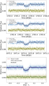 |
Fig. 1 Transits of TOI-1759 b observed by TESS. The blue points show the TESS photometry data around the three transits of TOI-1759 b. The bottom panel shows all data, with the times relative to the central time of each transit. The red lines show the best-fit transit model, and the green points show the residuals. |
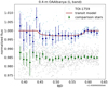 |
Fig. 2 Ground-based Ic -band differential photometry time series of a transit of TOI-1759 b obtained by the 0.4 m OAAlbanya observatory on May 20, 2020. The light blue points show relative fluxes of TOI-1759, and the dark blue points show weighted average bins with bin sizes of 0.01 days. The gray and green points show the relative fluxes for the comparison stars that we used in the differential photometry. The red line shows the best-fit transit model obtained from our analysis of the TESS data alone, as presented in Sect. 5. |
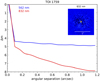 |
Fig. 3 Contrast ratio of TOI-1759 as a function of angular separation at 562 nm (blue line) and at 832 nm (red line) obtained from the ‘Alopeke/Gemini speckle imaging observations. |
2.4 SPIRou spectropolarimetry
TOI-1759 was observed by SPIRou5 under the large program SLS-WP26 (id P42, PI: Jean-François Donati). SPIRou is a stabilized high-resolution NIR spectropolarimeter (Donati et al. 2020) mounted on the 3.6 m CFHT atop Maunakea, Hawaii. It is designed for high-precision velocimetry to detect and characterize exoplanets and it provides a full coverage of the NIR spectrum from 950 nm to 2500 nm at a spectral resolving power of λ/Δλ ~ 70000.
A total of 218 spectra of TOI-1759 were obtained on 54 different epochs/nights, spanning 447 days from 2020-06-05T13:16:41 to 2021-08-26T08:51:39. Table F.1 presents the log of our SPIRou observations. These observations were carried out in the circular polarization mode (Stokes V), where each set of four exposures provides a polarimetric spectrum. Each exposure in the sequence corresponds to a different position of the two rotating Fresnel rhombs, where the sequence number of each exposure is also presented in Table F.1. On a few occasions, one exposure needed to be repeated due to passing clouds, implying more than four exposures per sequence. Under these circumstances, we select the set of four exposures with the highest signal-to-noise ratio (S/N). These observations were obtained at an average air mass of 1.47 with a dispersion of 0.12, and with an S/N per spectral element measured at 1670 nm ranging from 43 to 210, with a median of 184. The fourth exposure of one polari-metric sequence on 2021-06-19 has a low S/N, and could not be repeated due to degrading weather conditions. We therefore do not consider this sequence for polarimetry, but do use its three good exposures for spectroscopy.
A set of baseline calibration (flats, darks, comparison, and aligns) is obtained in the afternoon and in the morning of each night of observation with SPIRou. In addition, hot stars (A type) are observed nightly as telluric absorption standards. A set of bright inactive cool stars are also regularly observed as constant RV standards. We make use of these data to calibrate the measurements we extract from the SPIRou spectra, as discussed in more detail in Sect. 3.
3 SPIRou data reduction and analysis
3.1 APERO reduction
Our SPIRou data were reduced with the software A PipelinE to Reduce Observations (APERO7 v0.6.132; Cook et al., in prep.). APERO first performs some initial processing of the 4096×4096 pixel images of the HAWAII 4RG™ (H4RG), applying a series of procedures to correct detector effects, remove background thermal noise, and identify bad pixels and cosmic ray impacts.
It then uses exposures of a quartz halogen lamp (flat) to calculate the position of the 49 echelle spectral orders. It optimally extracts (Horne 1986) spectra of the two science channels (fibers A and B, fed by two orthogonal polarized beams) and the simultaneous calibration channel (fiber C). This APERO extraction takes into account the asymmetric shape of the instrument profile generated by the pupil slicer. Both a 2D order by order and 1D order-merged spectrum are produced for each channel of each scientific exposure. A blaze function is obtained from the flat-field exposures and a master flat is used to do the flux calibration.
The pixel-to-wavelength calibration is obtained from exposures of both a UNe hollow cathode lamp and a Fabry–Pérot etalon, as described in Hobson et al. (2021). This provides wavelengths in the rest frame of the observatory, but APERO also calculates the barycentric Earth radial velocity (BERV) and the barycentric Julian date (BJD) of each exposure using the code barycorrpy8 (Kanodia & Wright 2018; Wright & Eastman 2014). These can then be used to reference the wavelength and time to the barycentric frame of the solar system.
APERO calculates the spectrum of the telluric transmission using a novel technique based on a model obtained from the collection of standard star observations carried out since the beginning of SPIRou operations in 2018 and a fit made for each individual observation using the principal component analysis technique of Artigau et al. (2014). APERO also calculates the Stokes V (and where appropriate, Q and U) spectra using the method of Donati et al. (1997), as described in detail in Martioli et al. (2020).
3.2 Spectropolarimetry analysis
We further analyzed the SPIRou polarized spectra using the spirou-polarimetry9 code. The Stokes I, Stokes V, and null polarization spectra were compressed to one line profile using the least squares deconvolution (LSD) method of Donati et al. (1997). The line mask used in our LSD analysis of TOI-1759 was computed using the VALD catalog (Piskunov et al. 1995) and a MARCS model atmosphere (Gustafsson et al. 2008) with an effective temperature of 4000 K and surface gravity of log g = 5.0 dex. We select all lines deeper than 3% and with a Landé factor of geff > 0, for a total of 2460 atomic lines. Figure 4 displays the resulting LSD profiles at each observing epoch. Its Stokes V panel shows a significant and time-variable Zeeman signature, indicating the presence of magnetic field in this star, as will be explored in more detail in Sect. 4.3. Figure 5 shows the medians of all profiles in the time series, where the Zeeman signature is clearly evidenced in the “S” shape of the Stokes V profile.
To check the consistency of our measurements, we also obtained an independent polarimetric reduction and LSD analysis of our SPIRou data using the Libre-Esprit (LE) pipeline (Donati et al. 1997, Donati et al. 2020). The Stokes V profiles obtained from the APERO reduction show an RMS of 0.0039% (estimated in the outer regions of the profile, |υ − υsys| > 20 km s−1) and a semiamplitude of the median profile of 0.031%, and thus S/N = 8. The LE data show an RMS of 0.0016% and a semi-amplitude of 0.0061%, and thus a S/N = 4. The difference in the amplitude scale of these data sets is due to the different normalization factors adopted in the LSD analysis. However, the factor of two in detection significance stems from the noise characteristics that result from different reduction methods. A thorough comparison between the two pipelines is beyond the scope of this paper. Nevertheless, we analyzed and compared the results obtained from the two data sets, as will be shown in Sects. 4.3 and 4.4.
3.3 Radial velocities
Obtaining precise RVs from the Doppler shift of the stellar spectrum in the NIR is more challenging than in the optical domain. For instance, the NIR spectral domain of SPIRou is largely polluted by telluric absorption and sky emission lines, which affect measurements across the entire observed spectrum. The telluric correction inevitably changes the noise pattern and introduces more noise due to imperfect corrections. On the other hand, SPIRou’s NIR H4RG detector has artifacts such as evolving bad pixels, nonlinearity and persistence, which are not present in the same proportions in charged coupled devices (CCD). The challenges faced by high-precision velocimetry in the NIR were noted in other instruments with characteristics similar to SPIRou (Figueira et al. 2010; Carleo et al. 2016; Cale et al. 2019; Lafarga et al. 2020).
Here, we used two different methods to measure the RVs in the SPIRou data. First, we employed the well-established cross-correlation function (CCF) method of Pepe et al. (2002) with several specific data reduction procedures that are required to minimize the aforementioned problems found in the NIR observations, as presented in more detail in Sect. 3.4. Then, we used a line-by-line (LBL) method proposed by Dumusque (2018) and adapted by Artigau et al. (in prep.), which is summarized in Sect. 3.5. The LBL method seems to be more robust to the noise introduced by the telluric correction and also to the other artifacts of NIR observations.
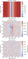 |
Fig. 4 Stokes I (top panel), Stokes V (middle panel), and null polarization (bottom panel) LSD profiles in the TOI-1759 SPIRou time series. |
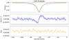 |
Fig. 5 Median of all LSD profiles in the TOI-1759 SPIRou time series. The top panel shows Stokes I LSD (red points) with a Voigt profile model fit (green line), the middle panel shows Stokes V (blue points) and the bottom panel shows the null polarization profile (orange points). |
3.4 CCF analysis
For the CCF analysis we use the package spirou-ccf10, which implements the CCF method to measure the RVs of the SPIRou spectra. The input data that we use in our analysis are the teluric corrected spectra calculated by the APERO pipeline (see Sect. 3.1). In the spirou-ccf package, several processing steps are done to minimize the strong systematic effects found in NIR data. Below is a summary of the procedures performed by our CCF analysis.
First, we selected an empirical CCF mask from a repository of masks obtained from observations of bright stars, which in this case is Gl 846, an M0.5V star that almost corresponds to the spectral type of TOI-1759. The mask selection is based on the criterion of proximity to the spectral type of the star. Each mask consists of a set of atomic and molecular lines, where the central wavelengths are obtained from the VALD catalog (Piskunov et al. 1995) and the line depths are obtained empirically from the template spectra of bright stars observed by SPIRou. Then we masked out sparsely sampled spectral ranges, which are defined as the ranges with "holes" (data flagged as NaN due to bad pixels or failed telluric correction) greater than 5 km/s. We applied a relativistic BERV correction to the wavelengths and resampled each spectrum to a constant 1.8 km s−1 grid by cubic spline interpolation. We combined all spectra into a high S/N template spectrum as illustrated in Fig. 6. To account for flux variations, we fit a low-order multiplicative polynomial for the flux of each spectrum, F(λ), on an order-by-order basis, as follows:
 (1)
(1)
where FT is the flux of the template spectrum, c0 is a constant offset, c1 is a scaling factor, and c2 accounts for smooth wavelength (λ) dependent variability. We applied a 3σ clip filter with σ being the median absolute deviation of each spectral element in the time domain. Figure 6 illustrates the dispersion of residuals that gives σ. We repeated this procedure of building a template spectrum to minimize deviations between data obtained at different times and the template spectrum.
Next, we fitted a polynomial to the continuum of each spectral order of the template spectrum by using an iterative sigma-clip algorithm as in the IRAF task noao.onedspec.continuum11 and we normalized each spectrum in the time series to the same continuum measured on the template spectrum. Finally, we calculated the order-by-order CCFs between the selected mask and the normalized template spectrum. We measured the systemic velocity (υsys) and the FWHM from a Gaussian fit to the mean CCF of the template spectrum, where we also calculated a CCF velocity range as υsys ± n × FWHM, where we set n = 7. We updated the CCF mask weights as  , as illustrated in Fig. 6, where
  is the mean dispersion in flux within the CCF velocity range around the line center and d is the line depth. Finally, we calculated the order-by-order CCF of each normalized spectrum in the time series using the same mask and the same velocity range for all spectra.
For each spectrum we calculated a weighted mean of the spectral order CCFs to build a final mean CCF per exposure. Figure 7 shows the weights given by  , where Q = ∫ (df(υ)/dυ)2dυ for f(υ) being the CCF value at a given velocity υ, and σCCF is the root mean square (RMS) dispersion of the CCF time series. Then, we calculated a CCF template by the median of the mean CCFs of all exposures as presented in Fig. 8. We applied a polynomial fit to the continuum of each mean CCF to match the template CCF (see Fig. 8). The continuum is defined as the points where |υ − υsys| < 1.5 × FWHM. Here, we also applied a 4σ clip filter to remove outliers from the CCF data. As an additional filter for outlier rejection, we excluded the CCF data from spectral orders in which less than half of the velocity bins are useful, that is, those with more than 50% of NaN values. We also excluded the CCF data from spectral orders that present a velocity shift greater than a given threshold of 3.0 km s−1. Then we recalculated the mean CCFs and a new template CCF from the clean CCF data. Finally, we calculated the final RV by least-square fitting for the velocity shift that best matches the mean CCF of an individual exposure to the template CCF.
The above procedure is applied to the spectra obtained from the sum of the flux of the two scientific fibers ‘A + B’ of SPIRou. For the simultaneous Fabry-Pérot spectrum obtained with the calibration fiber “C”, we applied the same procedure described above with the following changes: (a) we replaced the stellar mask by a mask containing the Fabry-Pérot lines; (b) we did not correct for the BERV; (c) we assumed a null systemic velocity; (d) we did not remove the continuum. The RVs obtained from the simultaneous calibration are compared to the RVs obtained for the same fiber in the Fabry–Pérot exposures taken during the night calibration sequence. In this way, we calculated the spectral shift (or instrumental drift) that occurred from the moment the wavelength calibration data were taken until the scientific exposure. This drift is finally used to correct the RVs obtained from the scientific fiber. The drift-corrected RVs of our CCF analysis are listed in the Table F.2. The RMS dispersion of uncorrected CCF RVs is 10.6 ms−1, and the RMS of drift-corrected data is 8.4 ms−1, showing that the drift correction accounts for an additional noise of about 6.4 ms−1 in our CCF data, assuming uncorrelated Gaussian noise. It should be noted that the approach presented here was critical to achieving m s−1 precision. Otherwise, when applying the CCF method in a more standardized way, the SPIRou RVs are completely dominated by systematic errors.
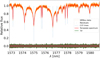 |
Fig. 6 Example of the reduced SPIRou spectra of TOI-1759 in the CCF analysis. Orange lines show the normalized SPIRou spectra for a small range in the H band. The red line shows the template spectrum, and the brown points show the residuals. The green lines show the measured ±3σ dispersion of the residuals, which are used by the sigma-clipping algorithm to reject outliers. The dashed blue lines show the central wavelengths of the CCF lines in the star’s frame of reference, where the depth of these lines is proportional to the CCF weight. |
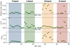 |
Fig. 7 CCF order weights. The top panel shows the relative weights applied to the CCFs of the SPIRou spectra of TOI-1759 as a function of the order number. Order numbering increases with wavelength, starting at zero. Photometric NIR bands are also marked with different colors and indicated at the top. The middle panel shows the Q factor that quantifies the RV content, and the lower panel shows the statistical weight as explained in the text. |
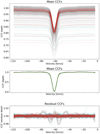 |
Fig. 8 CCF template matching. The top panel shows the weighted mean CCFs obtained for each spectrum of TOI-1759, where the color code shows the first epoch in dark blue and the last epoch in dark red. The middle panel shows the same CCFs normalized to the polynomial fit to match the template CCF (green line). The lower panel shows the CCFs with the template CCF subtracted. |
3.5 LBL analysis
The LBL method that we used in our analysis will be exhaustively presented in a forthcoming paper by Artigau et al. (in prep.). The method uses an approach similar to that used by Dumusque (2018) which draws on the Bouchy et al. (2001) formalism, in particular Eqs. (3) and (4) therein, and applies it to individual lines rather than the entire spectrum. As for the Bouchy et al. (2001) velocity measurement, one must have a noiseless template to compute a per-line velocity. This template is used to compare the residuals between the observed spectrum and the template to the derivative of the template. In practice, we use a high S/N combined spectrum of the star, assuming that any remaining noise contribution will be much smaller than the noise in the observation being considered. For TOI-1759, the template spectrum obtained from our observations does not have an S/N as good as in the templates of standard stars. Therefore, in this case, we use a template of G1846, which is a standard star of almost the same spectral type as TOI-1759.
The LBL algorithm provides one velocity per line (typically 16000 for an M dwarf observed with SPIRou), which must be combined into a single RV measurement. The per-line uncertainties vary from ~50 ms−1 for the best lines to tens of km s−1 for shallow features. In the absence of outlying points, a weighted sum would suffice to retrieve a per-spectrum velocity. As there are high-sigma outliers among lines, due to a number of plausible causes (cosmic rays hitting the array, error in telluric absorption correction), we opt for a finite-mixture model approach to derive a mean spectrum velocity. Lines either belong to a Gaussian distribution around the mean velocity with a sigma derived from the Bouchy et al. (2001) framework, or belong to a statistically flat distribution of outliers. In representative SPIRou data, 0.2% of lines are consistent with being outliers.
As in the CCF method, we also calculated the LBL RVs for the simultaneous calibration fiber to measure and correct for the instrumental drift. The drift-corrected RVs of our LBL analysis are also listed in the Table F.2. The RMS of uncorrected and drift-corrected LBL RVs are 9.5 ms−1 and 5.6 ms−1, respectively, showing that the instrumental drift contributed about 7.7 ms−1 to the noise in our LBL data. A comparative analysis of the RVs and the drifts obtained by the two methods is presented in Appendix B.
4 Stellar characterization
We carried out a study to derive the stellar properties and to characterize magnetic activity in TOI-1759, as will be detailed in the next sections. Table 2 presents a summary of the TOI-1759 stellar parameters.
4.1 Spectral energy distribution analysis
As a first determination of the basic stellar parameters, we performed an analysis of the broadband spectral energy distribution (SED) of the star together with the Gaia Early Data Release 3 parallax (with no systematic offset applied; see, e.g., Stassun & Torres 2021) in order to determine an empirical measurement of the stellar radius, following the procedures described in Stassun & Torres (2016), Stassun et al. (2017), and Stassun et al. (2018). We retrieved the JHKS magnitudes from 2MASS, the W1–W4 magnitudes from WISE, and the GBP G GRP magnitudes from Gaia. Together, the available photometry spans the stellar SED over the wavelength range 0.4–22 μm (see Table 2).
We performed a fit using NextGen stellar atmosphere models, with the effective temperature (Teff) and metallicity ([Fe/H]) as free parameters (the surface gravity, log g, has little influence on the broadband SED). We fixed the extinction, AV, to zero due to the proximity of the system. The resulting fit (Fig. 9) has a reduced χ2 of 1.2, with best-fit Teff = 4075 ± 75 K and [Fe/H] = 0.0 ± 0.3. Integrating the model SED gives the bolometric flux at Earth, Fbol = 1.765 ± 0.020 × 10⁻⁹ erg s−1 cm−2. Taking the Fbol and Teff together with the Gaia parallax, gives the stellar radius, R⋆ = 0.60 ± 0.03 R⊙.
4.2 Spectral synthesis analysis of the SPIRou template
As a second determination, we analyzed the normalized template SPIRou spectrum of TOI-1759 using the code iSpec12 (Blanco-Cuaresma et al. 2014; Blanco-Cuaresma 2019) and the radiative transfer code SPECTRUM (Gray & Corbally 2014). In this approach, a grid of synthetic spectra is computed using stellar atmospheric models from MARCS (Gustafsson et al. 2008) and a custom line list from the VALD catalog (1100–2400 nm) (Piskunov et al. 1995). The solar abundances are from Asplund et al. (2009). Here, we considered the range between 1100 nm and 1250 nm, where we used a total of 44 615 lines to produce the synthetic spectra. The best-fit synthetic spectra were obtained by minimizing the χ2, which gives us a reliable measurement of the fundamental parameters of TOI-1759. Figure 10 shows the SPIRou template spectrum and the best-fit synthetic spectrum of TOI-1759 obtained by our analysis. The best-fit stellar parameters are shown in Table 2. The spectroscopic parameters obtained in this analysis are consistent with those obtained in the SED analysis (see Sect. 4.1), although the uncertainty on Teff obtained here is larger, mainly due to the presence of activity (e.g., do Nascimento et al. 2016), whose complete characterization would require a detailed analysis beyond the scope of this work.
In addition, we obtained the spectroscopic parameters of TOI-1759 from a spectral characterization tool specifically developed to analyze SPIRou spectra of M dwarfs by Cristofari et al. (2022), which performs a least-squares search for best-fit parameters in a precomputed grid of spectra using both a grid of PHOENIX spectra from Husser et al. (2013) and a grid of spectra computed with Turbospectrum (Plez 2012) from MARCS (Gustafsson et al. 2008) model atmospheres. The PHOENIX grid gives Teff = 4046 ± 40 K, log g = 4.9 ± 0.2 dex, and [M/H] = +0.4 ± 0.2 dex, and the Turbospectrum+MARCS grid gives Teff = 3972 ± 40 K, log g = 4.5 ± 0.2 dex, and [M/H] = +0.1 ± 0.2 dex. These results agree with our SED fit and spectral synthesis analyses, showing an improvement in the uncertainty of Teff.
Summary of the stellar parameters of TOI-1759.
4.3 Magnetic activity, rotation, and age
To investigate the magnetic activity in TOI-1759, we calculated the disk-integrated longitudinal magnetic field, Bℓ, in the LSD profiles of SPIRou following the same prescription as in Donati et al. (1997), Moutou et al. (2020), and Martioli et al. (2020). Table F.3 presents the values of Bℓ for TOI-1759 from both APERO and LE reductions. The Bℓ corresponds to a measurement of the net magnetic field projected on the line-of-sight direction originated from magnetic regions in the visible hemisphere of the stellar photosphere. Since the spatial distribution of these magnetized features is likely to be heterogeneous, as later confirmed by our Zeeman-Doppler imaging (ZDI) analysis (see Sect. 4.4), Bℓ is expected to be modulated by the star’s rotation, allowing the rotation period to be derived if any periodicity is detected in its time series (e.g., Borra & Landstreet 1980; Morin et al. 2008; Moutou et al. 2017; Petit et al. 2021). Figure 11 shows the generalized Lomb–Scargle (GLS) periodogram (Zechmeister & Kürster 2009) for the Bℓ data calculated using the astropy.timeseries13 tool. We find the maximum power at a period of 35.7 d with a false alarm probability (FAP) below 0.001%.
The magnetic features of this star appear to evolve rapidly, as seen in our ZDI analysis (see Sect. 4.4), showing a change in the magnetic properties between 2020 and 2021. Therefore, this study required a flexible model to account for the variability of the stellar magnetic field. We employed a Gaussian process (GP) regression analysis (e.g., Haywood et al. 2014; Aigrain et al. 2015) using the code george14 (Ambikasaran et al. 2014), where we assume that the rotational modulated stellar activity signal in Bℓ is quasi-periodic (QP). Thus, we adopt a parameterized covariance function (or kernel) as in Angus et al. (2018), which is given by
![Mathematical equation: $k({{\rm{\tau }}_{ij}}) = {\alpha ^2}\exp \left[ { - {{{\rm{\tau }}_{ij}^2} \over {2{l^2}}} - {1 \over {{\beta ^2}}}{{\sin }^2}\left({{{\pi {\tau _{ij}}} \over {{P_{{\rm{rot}}}}}}} \right)} \right] + {\sigma ^2}{\delta _{ij}},$](/articles/aa/full_html/2022/04/aa42540-21/aa42540-21-eq7.png) (2)
(2)
where τij = ti − tj is the time difference between data points i and j, α2 is the amplitude of the covariance, l is the decay time, β is the smoothing factor, Prot is the star rotation period, and σ is the uncorrelated white noise, which adds a “jitter” term to the diagonal of the covariance matrix. This kernel combines a squared exponential component describing the overall covariance decay and a component that describes the periodic covariance structure, the amplitude of which is controlled by the smoothing factor. Values of β around 1, as we find for this object, correspond to a periodic variation without a strong harmonic content. As pointed out by Angus et al. (2018) the flexibility of this model can easily lead to overfitting of the data. Therefore, we adopted a prior distribution for the parameters (see Table 3) that restricts the search range to realistic values and avoids overfitting.
We use this GP framework to model the temporal variability of the Bℓ data, where we first fit the GP model parameters by the maximization of the likelihood function (Rasmussen & Williams 2006; Foreman-Mackey et al. 2017) using the package scipy.optimize, and then we sampled the posterior distribution of the free parameters using a Bayesian MCMC framework with the package emcee (Foreman-Mackey et al. 2013). We set the MCMC with 50 walkers, 1000 burn-in samples, and 5000 samples. The results of our analysis are illustrated in Fig. 12 where we present the Bℓ observed data and the best-fit GP model. Figure A.1 shows the MCMC samples and posterior distributions of the GP parameters. Table 3 shows the priors and best-fit parameters calculated by the medians and their 0.16 and 0.84 quantiles uncertainties. We performed the same analysis on both APERO and LE Bℓ data, which gives consistent GP parameters within 1σ. The APERO data are noisier, with an RMS of residuals of 2.3 G, while LE data give an RMS of 1.4 G. However, we adopted the star rotation period obtained with the APERO data, which has a posterior distribution that is more tightly constrained than in the LE data. In Fig. 13, we present the Bℓ data phase-folded to the best-fit star rotation period of Prot = 35.7 days, where we highlight the different rotation cycles using different colors.
We investigated if the periodicity found in the Bℓ data is also present in the TESS photometry data. Here, we considered the TESS flux data subtracted by the best-fit transit model using the parameters in Table 6 and binned by weighted average with a bin size of 0.1 days. Figure 14 shows the GLS periodogram with a highest power at a period of 10.9 days and two other smaller peaks at 6.2 days and 17.2 days. The rotation period of  days obtained from Bℓ does not show a significant peak in the TESS data, although there are significant peaks near its harmonics. However, as illustrated in the bottom panel of Fig. 14, the TESS data phase-folded with <ieq/> days show that different rotation cycles present some agreement in their overlapping features. This suggests that the surface of TOI-1759 has several small spots rather than large spots at some specific longitudes that would generate a simpler oscillatory modulation in the TESS light curve.
In Fig. 15, we present the results of our analysis of the TESS photometry data using the same QP GP framework, where we assumed the same priors listed in Table 3, except for the Prot, which we assumed a prior with the value obtained from Bℓ, that is, Prot = 𝒩(35.65,0.17). We tried to fit the TESS data alone but it does not place a strong constraint on the rotation period, as we found that the best-fit GP model converges to significantly different values of Prot with a small change in the quality of the fit, depending strongly on the choice of the initial values of Prot.
Finally, we can use the star’s rotation period that we obtained from Bℓ, Prot = 35.7 days, to estimate the system’s age via empirical gyrochronology relations. For example, we obtain an age of ≈2.9 Gyr via the relations of Mamajek & Hillenbrand (2008), although the star is slightly redder than the limits of applicability of those relations. Alternatively, we obtain an age of ≈3.9 Gyr with the M-dwarf relations of Engle & Guinan (2018), although the star is slightly hotter than the limits of applicability of those relations. A recent study of stellar clusters by Curtis et al. (2020) discovered a stalling in the spin-down of cool stars. Therefore, our age derivation above of 2.9–3.9 Gyr may be significantly underestimated. According to the results presented in Fig. 7 of Curtis et al. (2020), TOI-1759 seems to correspond better to a 6 ± 1 Gyr field star than to the younger members of clusters. Therefore, we conservatively estimate the empirical gyrochronology age of TOI-1759 to be in the range 3–7 Gyr.
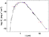 |
Fig. 9 SED of TOI-1759. Red symbols represent the observed photometric measurements, where the horizontal bars represent the effective width of the passband. Blue symbols are the model fluxes from the best-fit NextGen atmosphere model (black). |
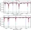 |
Fig. 10 Spectral synthesis analysis of TOI-1759. Black points show the normalized template SPIRou spectrum of TOI-1759, and the red line shows the best-fit synthetic spectrum with Teff = 4036 ± 100 K, log g = 5.1 ± 0.6 dex, and [M/H] = +0.2 ± 0.3 dex. The vertical blue lines show the positions of the lines of the main chemical species (as indicated on the labels) considered in our analysis. Our analysis included a total of 10242 lines within the spectral range 1137–1169 nm. Solid green lines show the residuals (observed minus synthetic). |
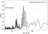 |
Fig. 11 GLS periodogram analysis of the longitudinal magnetic field (Bℓ) time series of TOI-1759. The dashed blue line shows the highest power at a period of 35.7 days. |
Best-fit parameters of a QP GP model obtained in our analysis of the stellar activity in the SPIRou Bℓ data.
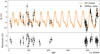 |
Fig. 12 GP analysis of the SPIRou Bℓ data. In the top panel, the black points show the observed Bℓ data and the orange line shows the best-fit QP GP model. The bottom panel shows the residuals with an RMS dispersion of 2.3 G. |
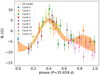 |
Fig. 13 SPIRou Bℓ data phase-folded with the best-fit period of 35.7 days. The data are represented by a different color for each rotation cycle, with the time of the zeroth cycle considered to be the time of the first SPIRou observation, that is, 2459006.063741 BJD. The orange-shaded region shows the best-fit GP model. |
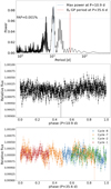 |
Fig. 14 GLS periodogram analysis of the TESS photometry data, with the best-fit transit model subtracted and binned by weighted average with a bin size of 0.1 days. The top panel shows the GLS periodogram, where the maximum power at 10.9 days is marked by the dashed blue line. The dashed red line shows the best-fit star rotation period of 35.7 days obtained in our analysis of the Bℓ data. The middle panel shows the TESS data phase-folded with a period of 10.9 days, and the bottom panel shows the TESS data phase-folded with a period of 35.7 days. The latter shows the data represented by a different color for each rotation cycle (as in Fig. 13), with the time of the zeroth cycle considered to be the time of the first SPIRou observation, that is, 2459006.063741 BJD. |
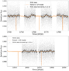 |
Fig. 15 GP analysis of the TESS photometry time series. The top panel shows the TESS data obtained in Sectors 16 and 17, and the bottom panel shows the data obtained in Sector 24. Black hollow circles show the TESS photometry in its original sampling, and the black points show the binned data, where each bin is calculated by the weighted mean within windows of 0.1 day. The orange line and shaded region show the best-fit GP model (multiplied by the transit model) and its uncertainty. |
4.4 Magnetic imaging
We reconstruct the large-scale magnetic field at the surface of TOI-1759 using ZDI. The algorithm models the magnetic topology as a combination of a poloidal and a toroidal component, which are both formulated via spherical-harmonics decomposition (Donati et al. 2006). An iterative comparison between synthetic and observed Stokes V profiles is performed until the maximum-entropy map at a given reduced χ2 level is found (for more details see Skilling & Bryan 1984; Donati & Brown 1997; Folsom et al. 2018).
We produced two ZDI maps from observations collected almost one year apart: between June 5, 2020, and December 24, 2020 (23 observations), and between the June 20, 2021, and August 26, 2021 (25 observations). The local Stokes I profiles are truncated at ±15 km s−1 from line center and modeled with a Voigt function defined by a Gaussian and Lorentzian width of 1.2 and 5.1 km s−1, respectively. As central wavelength and Landé factor, we use the normalization values of 1750 nm and 1.2. We adopted the linear limb darkening coefficient reported in Table 6 and let the spherical harmonics expansion reach the fifth degree in l, as higher degrees are unnecessary given the low value of the projected velocity (Morin et al. 2008). The observed and modeled Stokes V profiles are shown in Fig. 16.
The two maps of surface magnetic flux are shown in Fig. 17 and the map characteristics obtained from both APERO and LE datasets are reported in Table 4. Assuming solid body rotation, Prot = 35.7 days, veq sin(i) =0.84 km s−1, and stellar inclination = 80 deg (instead of 90 deg to prevent mirroring effects), we are able to fit the Stokes V profiles down to a reduced chi-square level of χ2 ~ 0.9 for LE and  for APERO. The latter indicates that APERO overestimates the error bars of its LSD profiles. This problem will be addressed in future works, therefore, we adopt here the ZDI results obtained from the LE profiles.
The magnetic topology is predominantly poloidal (99% of the magnetic energy) with the axisymmetric component decreasing from 75 ± 5% in 2020 to 54 ± 5% in 2021. We also observed a change in the tilt of the dipole field from 11 ± 5 deg in 2020 to 46 ± 5 deg in 2021. Our data also suggest a 20% increase in the intensity of the dipole component between 2020 and 2021; otherwise, the intensity of the mean magnetic field remained constant: the mean (Bm) and the dipole (Bdip) field strengths are 17 ± 3 G (2020) and 18 ± 4 G (2021), and −23 ± 5 G (2020) and −27 ± 5 G (2021), respectively. For comparison, the APERO data set gives no substantial change in the field strengths between the two seasons; however, the field strengths are about 1.5–2.0 times lower than the LE results, with an agreement within 2σ. This slight disagreement indicates that the different noise characteristics and normalization of the LSD profiles can probably bias the measurements of the field strengths.
To summarize, the magnetic topology of TOI-1759 is characterized by a weak (<20 G) and predominantly poloidal field, whose main axis of symmetry shows a variable inclination with time. This agrees with previous results on similar stars, for example Gl 205, whose spectral type, rotation periods, and magnetic properties are very similar to those of TOI-1759 (Hébrard et al. 2016).
Properties of the magnetic field of TOI-1759 obtained from our ZDI analysis of the 2020 and 2021 SPIRou data sets, using both the APERO and LE reduced data.
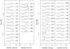 |
Fig. 16 Stokes V profiles (black lines) and their model (red lines) obtained with Prot = 35.7 d, veq sin (i)=0.84 km s−1 and i = 80 deg. The numbers at the right of each profile indicate the rotational cycle relative to the first Julian date of the time series of each season. The profiles are shifted vertically for better visualization. Left: 2020 time series. Right: 2021 time series. |
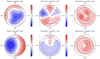 |
Fig. 17 ZDI maps of the recovered surface magnetic flux of TOI-1759 obtained from the best fit of the SPIRou data in 2020 (top panels) and 2021 (bottom panels). We show the radial (left panels), azimuthal (middle panels), and meridional (right panels) components of the magnetic field. The star is shown in a flattened polar projection, with the equator depicted as a bold circle and the 30° and 60° latitude parallels as dashed lines. Ticks around the star mark the rotational phases of our observations. The magnetic topology is predominantly poloidal, with the axisymmetric mode at an intermediate level. |
5 Planet characterization
We modeled the TESS photometry data with a baseline GP component to account for stellar activity as described in Sect. 4.3 multiplied by a transit model calculated using the BATMAN toolkit by Kreidberg (2015). The SPIRou RV data are modeled by the orbital reflex motion of the star caused by the planet, given by a Keplerian velocity as described in the Sect. 4 of Martioli et al. (2010). To perform a Bayesian MCMC joint analysis of the photometry and RV data sets, we build a global likelihood function that can be evaluated at each iteration of the MCMC sampler. Our likelihood function is given by the sum of the logarithm of the likelihood (log-likelihood) of the prior probability on the data and on the planet parameters plus the posterior probability of the trial models conditioned to the data. The general form of our likelihood function is given by
![Mathematical equation: $\ln {\cal L} = - {1 \over 2}\sum\limits_{i = 1}^N {\left[ {{{{{({y_i} - \mu)}^2}} \over {\sigma _i^2}} + \ln 2\pi \sigma _i^2} \right]} ,$](/articles/aa/full_html/2022/04/aa42540-21/aa42540-21-eq17.png) (3)
(3)
where N is the number of data points (or parameters), yi is a given data point (or parameter) and σi is its Gaussian uncertainty, and μ is the mean value. We sampled the posterior distribution of the model parameters using the emcee package. The chain was set with 50 walkers and 5000 MCMC steps, the firs 1000 of which we discard. To compare different data sets and model assumptions, we calculated the Bayesian information criterion (BIC), given by
 (4)
(4)
where k is the number of free parameters, n is the number of data points, and  is the likelihood for the best-fit model.
We first fit the transit model to the photometry data in the regions around the three transits of TOI-1759 b observed by TESS, as shown in Fig. 1. We defined the priors considering ranges that include only realistic values and the initial values were measured directly from the data as in Martioli et al. (2021). Then, we performed a joint analysis of photometry and RV data, setting the initial model with the planet parameters obtained from the transit analysis and uniform priors for the velocity semi-amplitude of Kp = 𝒰(0,∞)m s−1 and for the systemic velocity of vsys = 𝒰(-∞,∞) m s−1. We note that in this first analysis we do not include the activity model to the RV data. We first adopted a uniform prior for the orbital eccentricity and longitude of periastron, e = 𝒰(0,1) and ω = 𝒰(0,360) deg, and then we repeated the analysis assuming a circular orbit (e = 0). The best-fit eccentricities for the CCF and LBL data are 0.5 ± 0.2 and 0.2 ± 0.2, respectively. However, the BIC values obtained for a circular orbit, BICCCF = 19 896 and BICLBL = 19617, are lower than those obtained for a noncircular orbit, BICCCF = 19 917 and BICLBL = 19 645. This means that the information provided by the data does not justify increasing the number of model parameters, so we adopt a circular orbit from now on.
To investigate if an activity related signal modulates our RV data, we fitted a QP GP activity component to the RV data subtracted by the best-fit orbit model obtained above, where we assume a prior for the rotation period of Prot = 𝒩(35.65,0.17) days, as obtained in Sect. 4.3, and the same priors shown in Table 3 for the other GP parameters. Then we subtract this GP model from the original RVs and perform again a joint fit of the photometry and RV data. In Appendix C, we present the results of this analysis, where we show the MCMC samples and posterior distributions for the fit parameters and the RV data and each component of the best-fit model. Figure 18 shows the RV data and the best-fit orbit models phase-folded to the orbital period and with t0 being the time of transit (Tc). We notice that both orbits are in phase with the TESS transits. The BIC also improves with respect to the solution without a planet for all data sets, showing a consistent preference in favor of the orbit model. The Appendix D presents a periodogram analysis for the CCF and LBL data, both showing coherent peaks in the orbital period of P = 18.85 days. These peaks become more relevant when subtracting the GP model. As an additional test, we performed a joint analysis of the photometry, RV, and Bℓ data including the transit model, the RV orbit models and the GP activity model, simultaneously. However, since the GP model is more flexible than the orbit model, the GP tends to overfit the data, resulting in a less significant detection of the RV semi-amplitude. Our bisector analysis (see Appendix E) indicates an absence of activity-related signal in the RVs. Therefore, the GP model may actually be related to other spurious signals.
The Table 5 shows a comparison of the results obtained for the CCF and LBL data, and for a model with and without the GP component. We note that regardless of the method used (CCF or LBL) or whether or not the GP component is included, the velocity semi-amplitude is constrained and all planet parameters have posterior distributions that are consistent within 1σ. The GP activity component improves the final dispersion of the residuals and the BIC for both data sets. Our MCMC analysis assumes flat priors for the velocity semi-amplitude, Kp = 𝒰(0,100) m s−1; therefore, a null detection should result in a flat probability distribution toward zero. However, as illustrated in Figs. C.1 and C.2, Kp has a well-constrained posterior distribution at the upper and lower bounds for both data sets, defining an important constraint for the mass of TOI-1759 b.
With LBL+GP we obtained the lowest BIC value, with a velocity semi-amplitude of Kp = 2.3 ± 0.7 m s−1 and a RMS of residuals of 4.6 ms−1. Therefore, the final fit parameters we adopt are those obtained by the LBL RVs with GP activity model. The best-fit system parameters and derived quantities are summarized in Table 6. With a radius of 3.06 ± 0.22 R⊕ and a mass of 6.8 ± 1.0M⊕, TOI-1759 b is confirmed as a planet with a mean density of 1.3 ± 0.5 g cm−3; therefore, it is likely to be a gas-dominated sub-Neptune.
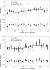 |
Fig. 18 TOI-1759 b orbit fit. The points in light gray show the SPIRou CCF (upper panel) and LBL (lower panel) RVs phase-folded at an orbital period of 18.850 days. Black points show weighted averages within a bin size of 0.05 (~0.95 days). The green lines and shaded regions show the best-fit models and their uncertainties for the orbit of TOI-1759 b. The residuals are displayed at the bottom of each panel, giving an RMS of 7.7 ms−1 and 4.6 ms−1 for CCF and LBL, respectively. |
Best-fit parameters obtained from our analyses using different combinations of RV data sets (CCF and LBL) and models (with and without a GP activity component).
6 TOI-1759 b as a potential target for atmospheric characterization
We considered the best-fit parameters from our analysis to calculate the habitable zone for TOI-1759 using the equations and data from Kopparapu et al. (2014), which gives an optimistic lower limit (recent Venus) at 0.24 au, and an upper limit (early Mars) at 0.61 au, with the runaway greenhouse limits (Mp = 1 M⊕) ranging between 0.31 au and 0.58 au. TOI-1759 b resides at an orbital distance of 0.1176 ± 0.0013 au and receives a flux of 6.4 times the flux incident on Earth, and therefore it is not inside the habitable zone. We estimated the equilibrium temperature for TOI-1759 b as in Heng & Demory (2013), assuming a uniform heat redistribution and an arbitrary geometric albedo of 0.1, which gives Teq = 433 ± 14 K, showing that this sub-Neptune is in a temperate region.
With a J magnitude of 8.7 for TOI-1759, the transits of TOI-1759 b can potentially be searched for atmospheric signatures. To characterize the potential for the detection of atmospheric absorption lines, we can evaluate the ratio between the atmospheric absorption depth and noise in the transit light curve. However, since the noise level will depend on the telescope, instrument, spectral range, etc., and the atmospheric absorption depth will depend on the species, abundances, number and oscillator strength of the searched lines, etc., at this point one can only calculate a relative S/N of detection to be compared with other planets and observed with the same instrument.
Here, we made the calculation in the J band, which is currently available with space and ground based facilities, and which includes the H2O bands observed in many studies of exo-planet atmospheres (e.g., Fraine et al. 2014; Benneke et al. 2019; Tsiaras et al. 2019; Mikal-Evans et al. 2021). The atmospheric absorption depth, which is the fraction of the stellar flux that is absorbed by the atmosphere during transit, is proportional to the area of the absorbing layer, which is given by the scale height of the atmosphere (H) times 2πRp, for Rp being the planet radius, and inversely proportional to the area of the stellar disk ( ). The noise is simply assumed to be proportional to the square root of the stellar flux given by
  , where mJ is the J magnitude of the star. The atmospheric scale height is given by kT/µgkT, where k is the Boltzmann constant, T is the atmosphere temperature, μ is the mean molar molecular mass, and g the planet gravity in the atmosphere. Finally, with, where Mp is the planet mass, we have an S/N of
  , in agreement with the transmission spectroscopic metric defined by Kempton et al. (2018) (see also, Cointepas et al. 2021).
We calculated the S/N expected for all known exoplanets transiting an M-type star, and normalized them to a value of 100 for the best case of AU Mic b. We used the catalog of exo-planets given by the Exoplanets Encyclopedia on August 1, 2021 (Schneider et al. 2011). For the J magnitudes, we used the tabulated values when available, or calculated theoretical values from the V magnitudes and the stars effective temperatures assuming a black-body spectrum. A star is considered to be an M-type if it is cataloged as such or if its effective temperature is between 2200 K and 4100 K. The result is shown in Fig. 19 where we plotted the S/N of the atmospheric signatures in the J band as a function of the planetary mass for known exoplanets orbiting M-type stars with masses between 4 and 14 M⊕. In this mass range, TOI-1759 b is the fourth best S/N after GJ3470 b, TOI-270 c, and TOI-270 d with an S/N about one-fourth that of GJ3470 b and half that of TOI-270 c.
In addition to the characterization of the deep atmosphere, TOI-1759 b provides interesting prospect in the search for evaporation signature. This planet shares many similar properties with GJ3470 b (planetary radius, equilibrium temperature, stellar type and effective temperature). GJ3470 b has shown a deep signature of an escaping atmosphere in Lyman-α (Bourrier et al. 2018). The main difference is that with a semimajor axis of 0.036 au, GJ3470 b is about three times closer to its star. There-fore, TOI-1759 b is farther to the evaporation limit (Lecavelier Des Etangs 2007).
To calculate the evaporation rate of TOI-1759 b, we used the hydrodynamic escape model from Allan & Vidotto (2019). This model calculates the optical depth for the XUV photons of the star – that is, the X-ray plus the energetic ultra-violet (EUV) radiation – which penetrate in the upper atmosphere of the planet. For simplicity, we assumed that the EUV photon energy is concentrated at 20 eV. These photons can then locally ionize neutral hydrogen atoms and the excess energy above the ionization threshold (i.e., >13.6 eV) is then used to heat the atmosphere, which expands and more easily evaporates. This bulk atmospheric outflow can potentially be detected in Lyman-α transit observations. One of the key inputs for the photoevapora-tion model is the high-energy XUV flux from the star incident on the planet. Given that the XUV flux is unknown for TOI-1759, we used empirical relations between magnetism and X-ray flux from Vidotto et al. (2014) to first estimate the X-ray flux of this star. Using the average magnetic fields reported in Table 2 and Fig. 6 from Vidotto et al. (2014), we estimated the X-ray flux of TOI-1759 to be ~6 × 10⁵ and ~1.5 × 10⁶ erg cm−2 s−1, if we consider an average field of 10 or 18 G, respectively. With these X-ray fluxes, we then used the empirical relations from (Johnstone et al. 2021, see their Eqs. (19) and (21)) to estimate the EUV flux of this star to be ~1.1 × 10⁶ and -2.1 × 10⁶ erg cm−2 s−1, which results in a total XUV flux of ~1.7 × 10⁶ and ~3.6 × 10⁶ erg cm−2 s−1 at the stellar surface. We note here that our values should be regarded as estimates, as the spread in empirical relations can be significant (see Vidotto et al. 2014).
Given the model dependence on the XUV stellar flux, it is worth comparing our estimated values with that from GJ3470. Using values from Bourrier et al. (2018), we find an XUV surface flux for GJ3470 of 7.7 × 10⁵ erg cm−2 s−1, which is comparable to that of TOI-1759, albeit a factor of few lower. Naively, we would expect that the faster rotation of GJ3470 (about a 20-day period) and its likely younger age (~2 Gyr; Bourrier et al. 2018) would have implied in a larger XUV surface flux of GJ3470, compared to that of TOI-1759, in contrast to what we found. This discrepancy could be due to the scatter in the relations we used here (see previous paragraph).
Using the lower-bound XUV flux value we found (~1.7 × 10⁶ erg s−1 cm−2), at the orbit of TOI-1759 b the incident stellar flux is 940 erg s−1 cm−2, which we adopted in our atmospheric escape model for TOI-1759 b. Assuming the planet has a hydrogen atmosphere, we find an escape rate of 1.4 × 10¹⁰ g s−1, which is remarkably similar to the rate derived for GJ3470 b (Bourrier et al. 2018). Given these similarities with GJ3470 b, TOI-1759 b might be an interesting target to observe neutral hydrogen escape.
In conclusion, the discovery of TOI-1759 b provides an interesting target with prospects for the observation of the deep atmosphere. However, given the possible high XUV flux, it is a potentially extremely interesting target in a search for escaping upper atmosphere in Lyman-α similar to GJ3470 b. Even the detection of the deep atmosphere will be in the capabilities of forthcoming facilities, which will aim at observing dozens of exoplanets atmospheres like the ESA space mission Ariel. In the sub-Neptune mass domain, it will be an interesting planet to be included in the first priority targets list.
Summary of the final fit parameters of TOI-1759 from the joint MCMC analysis of the TESS photometry and LBL SPIRou RVs.
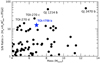 |
Fig. 19 S/N of the atmospheric signatures in the J band as a function of the planetary mass for exoplanets orbiting M-type stars with masses between 8 and 14 Earth mass. The S/Ns have been normalized to a reference S/N of 100 for the planet AU Mic b. In the considered mass range, the best S/Ns are obtained for the exoplanets GJ1214 b and GJ3470 b, with S/Ns of about half the one of AU Mic b. |
7 Conclusions
We have presented a detection of the transiting exoplanet TOI-1759 b and the characterization of the TOI-1759 system using TESS photometry and SPIRou/CFHT spectropolarimetry observations. The planet has a radius of 3.06 ± 0.22 R⊕ and a mass of 6.8 ± 2.0 M⊕ and therefore belongs in the sub-Neptune class, with a mean density of 1.3 ± 0.5 gcm−3. It orbits at a distance of 0.1176 ± 0.0013 au from a moderately active cool dwarf star, and its equilibrium temperature is 433 ± 14 K.
We measured the Doppler velocity shift of the star to a few m s−1 from our high-resolution NIR SPIRou spectra through both the CCF and LBL methods. These observations constrain the velocity semi-amplitude of the planet's orbit to within 3 σ. In a joint Bayesian MCMC analysis of the TESS photometry and SPIRou RVs, we fitted a Keplerian model of the planet’s RV orbit and a transit model to constrain the system's parameters.
In addition, the SPIRou circularly polarized spectra detect the Zeeman signature of the photospheric magnetic field of TOI-1759, which allowed us to characterize the magnetic properties of this star. We found that the longitudinal magnetic field is modulated by the star rotation, providing a star rotation period of  days. We reconstructed the magnetic map of the star with the ZDI technique, finding a predominantly poloidal field with an intermediate axisymmetry level. The mean magnetic field remained constant between 2020 and 2021, with a strength of Bmean = 18 ± 4G. However, we detected a change in the axisymmetric component from 75 ± 5% in 2020 to 54 ± 5% in 2021, and a change in the tilt and strength of the dipole field from 22 ± 5 deg and −23 ± 5 G in 2020 to 46 ± 5 deg and −27 ± 5 G in 2021.
Finally, we used our measurements of the stellar magnetic field and the system’s properties to estimate the photoevapora-tion rate in TOI-1759 b, which gives >1.4 × 10¹⁰ g s−1. This makes it a promising exoplanet to search for escaping upper atmosphere in Lyman-α transit observations and a potential target for the observation of the deep atmosphere. Therefore, TOI-1759 b is an important exoplanet for the understanding of the mechanisms that underlie the observed sub-Neptune radius desert.
Acknowledgements.
We acknowledge funding from the French National Research Agency (ANR) under contract number ANR18CE310019 (SPlaSH). This work is supported by the ANR in the framework of the Investissements d’Avenir program (ANR-15-IDEX-02), through the funding of the “Origin of Life” project of the Grenoble-Alpes University. T.V. and C.C. acknowledge funding from the Technologies for Exo-Planetary Science (TEPS) CREATE program and from the Fonds de Recherche du Quebec - Nature et technologies. J.F.D. acknowledges funding from the European Research Council (ERC) under the H2020 research & innovation programme (grant agreements 740651 New Worlds). A.A.V. acknowledges funding from the European Research Council (ERC) under the European Union's Horizon 2020 research and innovation programme (grant agreement no. 817540, ASTROFLOW). This paper includes data collected with the TESS mission, obtained from the MAST data archive at the Space Telescope Science Institute (STScI). We acknowledge the use of public TESS data from pipelines at the TESS Science Office and at the TESS Science Processing Operations Center. Resources supporting this work were provided by the NASA High-End Computing (HEC) Program through the NASA Advanced Supercomputing (NAS) Division at Ames Research Center for the production of the SPOC data products. Some of the observations in the paper made use of the High-Resolution Imaging instrument ‘Alopeke. ‘Alopeke was funded by the NASA Exoplanet Exploration Program and built at the NASA Ames Research Center by Steve B. Howell, Nic Scott, Elliott P. Horch, and Emmett Quigley. Data were reduced using a software pipeline originally written by Elliott Horch and Mark Everett. ‘Alopeke was mounted on the Gemini North telescope of the international Gemini Observatory, a program of NSF's OIR Lab, which is managed by the Association of Universities for Research in Astronomy (AURA) under a cooperative agreement with the National Science Foundation. on behalf of the Gemini partnership: the National Science Foundation (United States), National Research Council (Canada), Agencia Nacional de Investigación y Desarrollo (Chile), Ministerio de Ciencia, Tecnolog'ia e Innovación (Argentina), Ministério da Ciência, Tec-nologia, Inovações e Comunicações (Brazil), and Korea Astronomy and Space Science Institute (Republic of Korea).
Appendix A Bℓ GP posteriors
In this appendix we present the MCMC samples and posterior probability distributions of the QP GP activity model parameters, as defined in Section 4.3, obtained for the longitudinal magnetic field (Bℓ) time series. Figure A.1 illustrates these results.
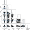 |
Fig. A.1 MCMC samples and the posterior distributions of parameters in the QP GP analysis of the stellar activity in the SPIRou Bℓ data. |
Appendix B Comparison between CCF and LBL RVs
We use two independent methods to calculate RVs, the CCF and the LBL. In this appendix we present a comparison between these two methods to verify the consistency between theirresults and if there is any residual systematics.
First, we compare the SPIRou instrumental drift measured from the simultaneous Fabry-Pérot spectrum in the calibration fiber“‘C”. Figure B.1 shows the drifts measured by the CCF method versus the drifts measured by the LBL method. We notice that there is a significant correlation of 0.96 between the drifts calculated by the two methods, with a median offset of −5.4 ± 1.9 ms−1 of the LBL with respect to the CCF drifts. These measurements show that SPIRou has an absolute drift that varies within a typical range of ±4 m s−1 (80th percentile), having much larger values (~ 30 − 40 m s−1) on some occasions due to sporadic jumps of the instrument. The RMS dispersion of 1.9 ms−1 for the differences between the two measurements is in good agreement with the expected internal uncertainties, which is on the order of 1 ms−1. The CCF drifts have a median error of 1.85 m s−1and the LBL drift errors are not computed in the current version.
Now we compare the RV measurements of TOI-1759 performed by both methods. Figure B.2 shows the time series of the difference between LBL and CCF RVs, where we did not detect any obvious systematics. The two methods provide RVs with a median offset of 79 m s−1 and a RMS dispersion of 6 m s−1. The latter is also in agreement with the expected dispersion of 7 m s−1, derived from the final RMS of 5.4 m s−1 and 4.6 m s−1, assuming uncorrelated errors.
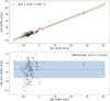 |
Fig. B.1 Comparison between CCF and LBL RV drifts measured from the Fabry-Pérot spectra obtained by the simultaneous calibration fiber of SPIRou observations of TOI-1759. The top panel shows the CCF drifts versus LBL drifts (black circles) as well as a linear fit to these quantities (solid green line) and its 1σ uncertainties (dashed red lines). The linear fit (parameters presented in the legend) shows a correlation of 0.96 between the CCF and LBL drifts. The bottom panel shows the differences between LBL and CCF drifts (black circles), the median (dashed blue line), and the 1σ = 1.9 ms−1 dispersion (shaded blue region). |
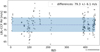 |
Fig. B.2 Comparison between CCF and LBL RVs of TOI-1759. The black circles show the differences between the LBL and CCF RVs, the dashed blue line shows the median difference, and the blue-shaded region represents the 1σ dispersion. |
Appendix C Fit models for CCF and LBL RVs
In this appendix we present the final results of our joint analysis of TESS photometry and SPIRou RV data, where we included a QP GP component to account for stellar activity in each data set as described in Section 5. Figures C.1 and C.2 show the MCMC samples and posterior distributions of the transit and RV model parameters, and Figures C.3 and C.4 show the fit models for the CCF and LBL RV data, respectively.
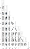 |
Fig. C.1 Pairs plot showing the MCMC samples and posterior distributions of the free parameters in our joint analysis of the TESS photometry and the SPIRou CCF RV data. The contours mark the 1σ, 2σ, and 3σ regions of the distribution. The blue crosses indicate the best-fit values for each parameter and the dashed vertical lines in the projected distributions show the median values and the 1σ uncertainty (34% on each side of the median). |
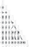 |
Fig. C.2 Same as Figure C.1 but for the LBL RV data. |
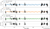 |
Fig. C.3 Best-fit models for the orbit of TOI-1759 b and the QP GP model for the stellar activity obtained from our MCMC joint analysis of the TESS photometry and the SPIRou CCF RV data. From top to bottom, panels show: (1) the orbit+GP model and the CCF RV data; (2) the GP model and the CCF RV data minus the orbit model; (3) the orbit model and the CCF RV data minus the GP model; and (d) the residuals, that is, the CCF RV data minus the orbit + GP model. |
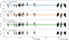 |
Fig. C.4 Same as Figure C.3 but for the LBL RV data. |
Appendix D Periodogram analysis of SPIRou RVs
In this appendix we present a periodogram analysis of the SPIRou rV data to inspect the significance of detection of the orbital RV signal of TOI-1759 b. Figure D.1 shows the conventional GLS periodogram, where we calculated the GLS periodogram for an increasing number of data points in a subset of our time series, starting at one-third, then two-thirds and then all data points. Both the CCF and LBL RVs show a peakat 18.85 d after removing the GP model, but a less significant peak when considering the data without subtracting the GP model. This low power reflects the marginal detection of the velocity semi-amplitude that we obtained in our analysis.
To further inspect the statistical significance of this faint signal, we employed the stacked Bayesian general Lomb-Scargle periodogram (SBGLSP) analysis of Mortier & Collier Cameron (2017). The result is illustrated in Figure D.2, where it shows that our RV data indeed presents a faint but coherent signal at 18.85 d, showing an increasing power with the number of observations. The signal becomes stronger and more evident after removing the GP model from both the CCF and LBL RVs. Finally, we calculated the S/N of the 18.85 d peak in the SBGLSP as a function of the number of observations. Figure D.3 shows that both data sets (CCF and LBL), with and without removing the GP model, present a monotonic increase in the S/N with the number of observations, which confirms the coherence of the detected signal.
Those analyses show that we detect the planet in the SPIRou data. The significance remains low, with detection of the RV semi-amplitude Kp between 3 and 5 σ according the values reported in Table 5. Still, the coherence of that signal and its agreement with both the period and the phase predicted fromthe TESS photometry allow us to conclude we significantly detect the planet.
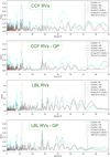 |
Fig. D.1 GLS periodogram analysis of SPIRou RVs of TOI-1759. The cyan, blue, and red lines show the GLS periodogram calculated for subsets containing one-third, two-thirds, and the entirety of the SPIRou RV data of TOI-1759, respectively. From top to bottom, panels show this analysis for CCF RVs, CCF RVs minus GP model, LBL RVs, and LBL RVs minus GP model. The removal of the GP model shows an improvement in the signature of the planet, expected at a period of 18.850 d (dashed green line). The dashed orange and blue lines show the periods found by our GP analysis of the TESS data and Bℓ data, respectively. |
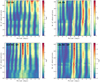 |
Fig. D.2 SBGLSP analysis of the SPIRou RVs of TOI-1759. Each panel shows a color map of the power in the SBGLSP for each RV data set. The vertical dashed lines show the orbital period of TOI-1759 b. |
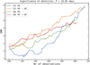 |
Fig. D.3 Significance of detection of the TOI-1759 b orbit RV signal at 18.85 d in the SBGLSP analysis. Each curve represents the S/N as a function of the number of observations. The S/N is calculated as the ratio between the SBGLSP power at 18.85 d and the noise in the periodogram. There is a monotonic increase in the S/N with the number of observations for all data sets, showing the coherent nature of the signal detected. |
Appendix E Bisector analysis
To check whether the RVs are correlated with some changes in the line profiles we use the bisector analysis as in Queloz et al. (2001) and Boisse et al. (2009), where we calculate the bisector span, given by Bspan = vt - vb, where vt is the velocity shift of the bisector at the top of the CCF (55% < depth < 80%) and vb is the velocity shift of the bisector at the bottom of the CCF (20% < depth < 40%). Figure E.1 shows that there is no significant correlation between Bspan and the RVs, with a global Pearson-r coefficient of -0.10 and -0.01 and a p-value of 0.17 and 0.85, for CCF and LBL, respectively. Therefore, the RVs do not vary significantly with the shape of the line profiles. Although our bisector analysis indicates the absence of an activity-related signal in the RVs of TOI-1759, further validation of this method in active stars is yet to be done with SPIRou.
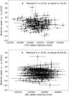 |
Fig. E.1 Bisector span versus SPIRou RVs. The top panel shows the CCF RVs, and the bottom panel shows the LBL RVs, where we verify that there is no correlation between these quantities and the bisector span. The blue lines show a linear fit, and the legends show the Pearson-r coefficients and their corresponding p-values. |
Appendix F SPIRou log of observations, RVs, and Bℓ data
This appendix presents the log of SPIRou observations of TOI-1759 in Table F.1, the CCF and LBL RVs in Table F.2, and the longitudinal magnetic field (Bℓ) data in Table F.3.
Log of SPIRou observations of TOI-1759.
CCF and LBL SPIRou RVs minus the median velocities of −61072.6 and −60992.9 ms−1, respectively.
Longitudinal magnetic field data of TOI-1759 measured by SPIRou calculated both from APERO and LE reduction.
References
- Aigrain, S., Hodgkin, S. T., Irwin, M. J., Lewis, J. R., & Roberts, S. J. 2015, MNRAS, 447, 2880 [NASA ADS] [CrossRef] [Google Scholar]
- Allan, A., & Vidotto, A. A. 2019, MNRAS, 490, 3760 [Google Scholar]
- Ambikasaran, S., Foreman-Mackey, D., Greengard, L., Hogg, D. W., & O’Neil, M. 2014, IEEE Trans. Pattern Anal. Mach. Intell. 38, 252 [Google Scholar]
- Angus, R., Morton, T., Aigrain, S., Foreman-Mackey, D., & Rajpaul, V. 2018, MNRAS, 474, 2094 [Google Scholar]
- Artigau, É., Astudillo-Defru, N., Delfosse, X., et al. 2014, SPIE Conf. Ser., 9149, 914905 [NASA ADS] [Google Scholar]
- Asplund, M., Grevesse, N., Sauval, A. J., & Scott, P. 2009, ARA&A, 47, 481 [NASA ADS] [CrossRef] [Google Scholar]
- Benneke, B., Wong, I., Piaulet, C., et al. 2019, ApJ, 887, L14 [Google Scholar]
- Blanco-Cuaresma, S. 2019, MNRAS, 486, 2075 [Google Scholar]
- Blanco-Cuaresma, S., Soubiran, C., Heiter, U., & Jofré, P. 2014, A&A, 569, A111 [CrossRef] [EDP Sciences] [Google Scholar]
- Boisse, I., Moutou, C., Vidal-Madjar, A., et al. 2009, A&A, 495, 959 [NASA ADS] [CrossRef] [EDP Sciences] [Google Scholar]
- Borra, E. F., & Landstreet, J. D. 1980, ApJS, 42, 421 [Google Scholar]
- Bouchy, F., Pepe, F., & Queloz, D. 2001, A&A, 374, 733 [NASA ADS] [CrossRef] [EDP Sciences] [Google Scholar]
- Bourrier, V., Lecavelier des Etangs, A., Ehrenreich, D., et al. 2018, A&A, 620, A147 [NASA ADS] [CrossRef] [EDP Sciences] [Google Scholar]
- Caldwell, D. A., Tenenbaum, P., Twicken, J. D., et al. 2020, RNAAS, 4, 201 [NASA ADS] [Google Scholar]
- Cale, B., Plavchan, P., LeBrun, D., et al. 2019, AJ, 158, 170 [Google Scholar]
- Carleo, I., Sanna, N., Gratton, R., et al. 2016, Exp. Astron., 41, 351 [NASA ADS] [CrossRef] [Google Scholar]
- Ciardi, D. R., Beichman, C. A., Horch, E. P., & Howell, S. B. 2015, ApJ, 805, 16 [NASA ADS] [CrossRef] [Google Scholar]
- Cloutier, R., & Menou, K. 2020, AJ, 159, 211 [NASA ADS] [CrossRef] [Google Scholar]
- Cointepas, M., Almenara, J. M., Bonfils, X., et al. 2021, A&A, 650, A145 [NASA ADS] [CrossRef] [EDP Sciences] [Google Scholar]
- Cristofari, P. I., Donati, J.-F., Masseron, T., et al. 2022, MNRAS, 511, 1893 [NASA ADS] [CrossRef] [Google Scholar]
- Curtis, J. L., Agüeros, M. A., Matt, S. P., et al. 2020, ApJ, 904, 140 [Google Scholar]
- Cutri, R. M., Skrutskie, M. F., van Dyk, S., et al. 2003, VizieR Online Data Catalog: II/246 [Google Scholar]
- do Nascimento, J. D. J., Vidotto, A. A., Petit, P., et al. 2016, ApJ, 820, L15 [NASA ADS] [CrossRef] [Google Scholar]
- Donati, J. F., & Brown, S. F. 1997, A&A, 326, 1135 [Google Scholar]
- Donati, J. F., Semel, M., Carter, B. D., Rees, D. E., & Collier Cameron, A. 1997, MNRAS, 291, 658 [Google Scholar]
- Donati, J.-F., Forveille, T., Collier Cameron, A., et al. 2006, Science, 311, 633 [Google Scholar]
- Donati, J. F., Kouach, D., Moutou, C., et al. 2020, MNRAS, 498, 5684 [Google Scholar]
- Dumusque, X. 2018, A&A, 620, A47 [NASA ADS] [CrossRef] [EDP Sciences] [Google Scholar]
- Engle, S. G., & Guinan, E. F. 2018, RNAAS, 2, 34 [NASA ADS] [Google Scholar]
- Figueira, P., Pepe, F., Melo, C. H. F., et al. 2010, A&A, 511, A55 [NASA ADS] [CrossRef] [EDP Sciences] [Google Scholar]
- Folsom, C. P., Bouvier, J., Petit, P., et al. 2018, MNRAS, 474, 4956 [NASA ADS] [CrossRef] [Google Scholar]
- Foreman-Mackey, D., Hogg, D. W., Lang, D., & Goodman, J. 2013, PASP, 125, 306 [Google Scholar]
- Foreman-Mackey, D., Agol, E., Angus, R., & Ambikasaran, S. 2017, AJ, 154, 220 [NASA ADS] [CrossRef] [Google Scholar]
- Fraine, J., Deming, D., Benneke, B., et al. 2014, Nature, 513, 526 [Google Scholar]
- Fulton, B. J., & Petigura, E. A. 2018, AJ, 156, 264 [Google Scholar]
- Gaia Collaboration (Brown, A. G. A., et al.) 2021, A&A, 649, A1 [NASA ADS] [CrossRef] [EDP Sciences] [Google Scholar]
- Giacalone, S., Dressing, C. D., Jensen, E. L. N., et al. 2021, AJ, 161, 24 [Google Scholar]
- Ginzburg, S., Schlichting, H. E., & Sari, R. 2018, MNRAS, 476, 759 [Google Scholar]
- Gray, R. O., & Corbally, C. J. 2014, AJ, 147, 80 [CrossRef] [Google Scholar]
- Guerrero, N. M., Seager, S., Huang, C. X., et al. 2021, ApJS, 254, 39 [NASA ADS] [CrossRef] [Google Scholar]
- Gupta, A., & Schlichting, H. E. 2021, MNRAS, 504, 4634 [NASA ADS] [CrossRef] [Google Scholar]
- Gustafsson, B., Edvardsson, B., Eriksson, K., et al. 2008, A&A, 486, 951 [NASA ADS] [CrossRef] [EDP Sciences] [Google Scholar]
- Haywood, R. D., Collier Cameron, A., Queloz, D., et al. 2014, MNRAS, 443, 2517 [Google Scholar]
- Hébrard, É. M., Donati, J. F., Delfosse, X., et al. 2016, MNRAS, 461, 1465 [CrossRef] [Google Scholar]
- Heng, K., & Demory, B.-O. 2013, ApJ, 777, 100 [NASA ADS] [CrossRef] [Google Scholar]
- Hobson, M. J., Bouchy, F., Cook, N. J., et al. 2021, A&A, 648, A48 [NASA ADS] [CrossRef] [EDP Sciences] [Google Scholar]
- Horne, K. 1986, PASP, 98, 609 [Google Scholar]
- Howell, S. B., Everett, M. E., Sherry, W., Horch, E., & Ciardi, D. R. 2011, AJ, 142, 19 [Google Scholar]
- Husser, T. O., Wende-von Berg, S., Dreizler, S., et al. 2013, A&A, 553, A6 [NASA ADS] [CrossRef] [EDP Sciences] [Google Scholar]
- Jenkins, J. M. 2002, ApJ, 575, 493 [Google Scholar]
- Jenkins, J. M., Chandrasekaran, H., McCauliff, S. D., et al. 2010, SPIE Conf. Ser., 7740, 77400D [Google Scholar]
- Jenkins, J. M., Twicken, J. D., McCauliff, S., et al. 2016, in Proc. SPIE, 9913, Software and Cyberinfrastructure for Astronomy IV, 99133E [Google Scholar]
- Johnstone, C. P., Bartel, M., & Güdel, M. 2021, A&A, 649, A96 [EDP Sciences] [Google Scholar]
- Kanodia, S., & Wright, J. 2018, RNAAS, 2, 4 [NASA ADS] [Google Scholar]
- Kempton, E. M. R., Bean, J. L., Louie, D. R., et al. 2018, PASP, 130, 114401 [Google Scholar]
- Kopparapu, R. K., Ramirez, R. M., SchottelKotte, J., et al. 2014, ApJ, 787, L29 [Google Scholar]
- Kreidberg, L. 2015, PASP, 127, 1161 [Google Scholar]
- Lafarga, M., Ribas, I., Lovis, C., et al. 2020, A&A, 636, A36 [NASA ADS] [CrossRef] [EDP Sciences] [Google Scholar]
- Lecavelier Des Etangs, A. 2007, A&A, 461, 1185 [NASA ADS] [CrossRef] [EDP Sciences] [Google Scholar]
- Li, J., Tenenbaum, P., Twicken, J. D., et al. 2019, PASP, 131, 024506 [NASA ADS] [CrossRef] [Google Scholar]
- Lopez, E. D., & Fortney, J. J. 2013, ApJ, 776, 2 [Google Scholar]
- Loyd, R. O. P., Shkolnik, E. L., Schneider, A. C., et al. 2020, ApJ, 890, 23 [NASA ADS] [CrossRef] [Google Scholar]
- Mamajek, E. E., & Hillenbrand, L. A. 2008, ApJ, 687, 1264 [Google Scholar]
- Mann, A. W., Feiden, G. A., Gaidos, E., Boyajian, T., & von Braun, K. 2015, ApJ, 804, 64 [Google Scholar]
- Martioli, E., McArthur, B. E., Benedict, G. F., et al. 2010, ApJ, 708, 625 [NASA ADS] [CrossRef] [Google Scholar]
- Martioli, E., Hébrard, G., Moutou, C., et al. 2020, A&A, 641, L1 [EDP Sciences] [Google Scholar]
- Martioli, E., Hébrard, G., Correia, A. C. M., Laskar, J., & Lecavelier des Etangs, A. 2021, A&A, 649, A177 [NASA ADS] [CrossRef] [EDP Sciences] [Google Scholar]
- Mikal-Evans, T., Crossfield, I. J. M., Benneke, B., et al. 2021, AJ, 161, 18 [Google Scholar]
- Morin, J., Donati, J. F., Petit, P., et al. 2008, MNRAS, 390, 567 [Google Scholar]
- Mortier, A., & Collier Cameron, A. 2017, A&A, 601, A110 [NASA ADS] [CrossRef] [EDP Sciences] [Google Scholar]
- Moutou, C., Hébrard, E. M., Morin, J., et al. 2017, MNRAS, 472, 4563 [NASA ADS] [CrossRef] [Google Scholar]
- Moutou, C., Dalal, S., Donati, J. F., et al. 2020, A&A, 642, A72 [NASA ADS] [CrossRef] [EDP Sciences] [Google Scholar]
- Owen, J. E., & Wu, Y. 2013, ApJ, 775, 105 [Google Scholar]
- Owen, J. E., & Wu, Y. 2017, ApJ, 847, 29 [Google Scholar]
- Pepe, F., Mayor, M., Galland, F., et al. 2002, A&A, 388, 632 [NASA ADS] [CrossRef] [EDP Sciences] [Google Scholar]
- Petit, P., Folsom, C. P., Donati, J. F., et al. 2021, A&A, 648, A55 [NASA ADS] [CrossRef] [EDP Sciences] [Google Scholar]
- Piskunov, N. E., Kupka, F., Ryabchikova, T. A., Weiss, W. W., & Jeffery, C. S. 1995, A&AS, 112, 525 [Google Scholar]
- Plez, B. 2012, Turbospectrum: Code for spectral synthesis [Google Scholar]
- Queloz, D., Henry, G. W., Sivan, J. P., et al. 2001, A&A, 379, 279 [NASA ADS] [CrossRef] [EDP Sciences] [Google Scholar]
- Rasmussen, C. E., & Williams, C. K. I. 2006, Gaussian Processes for Machine Learning [Google Scholar]
- Ricker, G. R., Winn, J. N., Vanderspek, R., et al. 2015, J. Astron. Telescopes Instrum. Syst., 1, 014003 [Google Scholar]
- Rogers, J. G., & Owen, J. E. 2021, MNRAS, 503, 1526 [NASA ADS] [CrossRef] [Google Scholar]
- Schneider, J., Dedieu, C., Le Sidaner, P., Savalle, R., & Zolotukhin, I. 2011, A&A, 532, A79 [NASA ADS] [CrossRef] [EDP Sciences] [Google Scholar]
- Skilling, J., & Bryan, R. K. 1984, MNRAS, 211, 111 [NASA ADS] [CrossRef] [Google Scholar]
- Smith, J. C., Stumpe, M. C., Van Cleve, J. E., et al. 2012, PASP, 124, 1000 [Google Scholar]
- Stassun, K. G., & Torres, G. 2016, AJ, 152, 180 [Google Scholar]
- Stassun, K. G., & Torres, G. 2021, ApJ, 907, L33 [NASA ADS] [CrossRef] [Google Scholar]
- Stassun, K. G., Collins, K. A., & Gaudi, B. S. 2017, AJ, 153, 136 [Google Scholar]
- Stassun, K. G., Corsaro, E., Pepper, J. A., & Gaudi, B. S. 2018, AJ, 155, 22 [Google Scholar]
- Stumpe, M. C., Smith, J. C., Van Cleve, J. E., et al. 2012, PASP, 124, 985 [Google Scholar]
- Stumpe, M. C., Smith, J. C., Catanzarite, J. H., et al. 2014, PASP, 126, 100 [Google Scholar]
- Tsiaras, A., Waldmann, I. P., Tinetti, G., Tennyson, J., & Yurchenko, S. N. 2019, Nat. Astron., 3, 1086 [Google Scholar]
- Twicken, J. D., Catanzarite, J. H., Clarke, B. D., et al. 2018, PASP, 130, 064502 [Google Scholar]
- Venturini, J., Guilera, O. M., Haldemann, J., Ronco, M. P., & Mordasini, C. 2020, A&A, 643, L1 [NASA ADS] [CrossRef] [EDP Sciences] [Google Scholar]
- Vidotto, A. A., Gregory, S. G., Jardine, M., et al. 2014, MNRAS, 441, 2361 [Google Scholar]
- Wright, J. T., & Eastman, J. D. 2014, PASP, 126, 838 [Google Scholar]
- Wright, E. L., Eisenhardt, P. R. M., Mainzer, A. K., et al. 2010, AJ, 140, 1868 [Google Scholar]
- Zechmeister, M., & Kürster, M. 2009, A&A, 496, 577 [CrossRef] [EDP Sciences] [Google Scholar]
- Zeng, L., Jacobsen, S. B., Sasselov, D. D., et al. 2019, Proc. Natl. Acad. Sci. U.S.A., 116, 9723 [Google Scholar]
All Tables
Best-fit parameters of a QP GP model obtained in our analysis of the stellar activity in the SPIRou Bℓ data.
Properties of the magnetic field of TOI-1759 obtained from our ZDI analysis of the 2020 and 2021 SPIRou data sets, using both the APERO and LE reduced data.
Best-fit parameters obtained from our analyses using different combinations of RV data sets (CCF and LBL) and models (with and without a GP activity component).
Summary of the final fit parameters of TOI-1759 from the joint MCMC analysis of the TESS photometry and LBL SPIRou RVs.
CCF and LBL SPIRou RVs minus the median velocities of −61072.6 and −60992.9 ms−1, respectively.
Longitudinal magnetic field data of TOI-1759 measured by SPIRou calculated both from APERO and LE reduction.
All Figures
|
Fig. 1 Transits of TOI-1759 b observed by TESS. The blue points show the TESS photometry data around the three transits of TOI-1759 b. The bottom panel shows all data, with the times relative to the central time of each transit. The red lines show the best-fit transit model, and the green points show the residuals. |
| In the text | |
|
Fig. 2 Ground-based Ic -band differential photometry time series of a transit of TOI-1759 b obtained by the 0.4 m OAAlbanya observatory on May 20, 2020. The light blue points show relative fluxes of TOI-1759, and the dark blue points show weighted average bins with bin sizes of 0.01 days. The gray and green points show the relative fluxes for the comparison stars that we used in the differential photometry. The red line shows the best-fit transit model obtained from our analysis of the TESS data alone, as presented in Sect. 5. |
| In the text | |
|
Fig. 3 Contrast ratio of TOI-1759 as a function of angular separation at 562 nm (blue line) and at 832 nm (red line) obtained from the ‘Alopeke/Gemini speckle imaging observations. |
| In the text | |
|
Fig. 4 Stokes I (top panel), Stokes V (middle panel), and null polarization (bottom panel) LSD profiles in the TOI-1759 SPIRou time series. |
| In the text | |
|
Fig. 5 Median of all LSD profiles in the TOI-1759 SPIRou time series. The top panel shows Stokes I LSD (red points) with a Voigt profile model fit (green line), the middle panel shows Stokes V (blue points) and the bottom panel shows the null polarization profile (orange points). |
| In the text | |
|
Fig. 6 Example of the reduced SPIRou spectra of TOI-1759 in the CCF analysis. Orange lines show the normalized SPIRou spectra for a small range in the H band. The red line shows the template spectrum, and the brown points show the residuals. The green lines show the measured ±3σ dispersion of the residuals, which are used by the sigma-clipping algorithm to reject outliers. The dashed blue lines show the central wavelengths of the CCF lines in the star’s frame of reference, where the depth of these lines is proportional to the CCF weight. |
| In the text | |
|
Fig. 7 CCF order weights. The top panel shows the relative weights applied to the CCFs of the SPIRou spectra of TOI-1759 as a function of the order number. Order numbering increases with wavelength, starting at zero. Photometric NIR bands are also marked with different colors and indicated at the top. The middle panel shows the Q factor that quantifies the RV content, and the lower panel shows the statistical weight as explained in the text. |
| In the text | |
|
Fig. 8 CCF template matching. The top panel shows the weighted mean CCFs obtained for each spectrum of TOI-1759, where the color code shows the first epoch in dark blue and the last epoch in dark red. The middle panel shows the same CCFs normalized to the polynomial fit to match the template CCF (green line). The lower panel shows the CCFs with the template CCF subtracted. |
| In the text | |
|
Fig. 9 SED of TOI-1759. Red symbols represent the observed photometric measurements, where the horizontal bars represent the effective width of the passband. Blue symbols are the model fluxes from the best-fit NextGen atmosphere model (black). |
| In the text | |
|
Fig. 10 Spectral synthesis analysis of TOI-1759. Black points show the normalized template SPIRou spectrum of TOI-1759, and the red line shows the best-fit synthetic spectrum with Teff = 4036 ± 100 K, log g = 5.1 ± 0.6 dex, and [M/H] = +0.2 ± 0.3 dex. The vertical blue lines show the positions of the lines of the main chemical species (as indicated on the labels) considered in our analysis. Our analysis included a total of 10242 lines within the spectral range 1137–1169 nm. Solid green lines show the residuals (observed minus synthetic). |
| In the text | |
|
Fig. 11 GLS periodogram analysis of the longitudinal magnetic field (Bℓ) time series of TOI-1759. The dashed blue line shows the highest power at a period of 35.7 days. |
| In the text | |
|
Fig. 12 GP analysis of the SPIRou Bℓ data. In the top panel, the black points show the observed Bℓ data and the orange line shows the best-fit QP GP model. The bottom panel shows the residuals with an RMS dispersion of 2.3 G. |
| In the text | |
|
Fig. 13 SPIRou Bℓ data phase-folded with the best-fit period of 35.7 days. The data are represented by a different color for each rotation cycle, with the time of the zeroth cycle considered to be the time of the first SPIRou observation, that is, 2459006.063741 BJD. The orange-shaded region shows the best-fit GP model. |
| In the text | |
|
Fig. 14 GLS periodogram analysis of the TESS photometry data, with the best-fit transit model subtracted and binned by weighted average with a bin size of 0.1 days. The top panel shows the GLS periodogram, where the maximum power at 10.9 days is marked by the dashed blue line. The dashed red line shows the best-fit star rotation period of 35.7 days obtained in our analysis of the Bℓ data. The middle panel shows the TESS data phase-folded with a period of 10.9 days, and the bottom panel shows the TESS data phase-folded with a period of 35.7 days. The latter shows the data represented by a different color for each rotation cycle (as in Fig. 13), with the time of the zeroth cycle considered to be the time of the first SPIRou observation, that is, 2459006.063741 BJD. |
| In the text | |
|
Fig. 15 GP analysis of the TESS photometry time series. The top panel shows the TESS data obtained in Sectors 16 and 17, and the bottom panel shows the data obtained in Sector 24. Black hollow circles show the TESS photometry in its original sampling, and the black points show the binned data, where each bin is calculated by the weighted mean within windows of 0.1 day. The orange line and shaded region show the best-fit GP model (multiplied by the transit model) and its uncertainty. |
| In the text | |
|
Fig. 16 Stokes V profiles (black lines) and their model (red lines) obtained with Prot = 35.7 d, veq sin (i)=0.84 km s−1 and i = 80 deg. The numbers at the right of each profile indicate the rotational cycle relative to the first Julian date of the time series of each season. The profiles are shifted vertically for better visualization. Left: 2020 time series. Right: 2021 time series. |
| In the text | |
|
Fig. 17 ZDI maps of the recovered surface magnetic flux of TOI-1759 obtained from the best fit of the SPIRou data in 2020 (top panels) and 2021 (bottom panels). We show the radial (left panels), azimuthal (middle panels), and meridional (right panels) components of the magnetic field. The star is shown in a flattened polar projection, with the equator depicted as a bold circle and the 30° and 60° latitude parallels as dashed lines. Ticks around the star mark the rotational phases of our observations. The magnetic topology is predominantly poloidal, with the axisymmetric mode at an intermediate level. |
| In the text | |
|
Fig. 18 TOI-1759 b orbit fit. The points in light gray show the SPIRou CCF (upper panel) and LBL (lower panel) RVs phase-folded at an orbital period of 18.850 days. Black points show weighted averages within a bin size of 0.05 (~0.95 days). The green lines and shaded regions show the best-fit models and their uncertainties for the orbit of TOI-1759 b. The residuals are displayed at the bottom of each panel, giving an RMS of 7.7 ms−1 and 4.6 ms−1 for CCF and LBL, respectively. |
| In the text | |
|
Fig. 19 S/N of the atmospheric signatures in the J band as a function of the planetary mass for exoplanets orbiting M-type stars with masses between 8 and 14 Earth mass. The S/Ns have been normalized to a reference S/N of 100 for the planet AU Mic b. In the considered mass range, the best S/Ns are obtained for the exoplanets GJ1214 b and GJ3470 b, with S/Ns of about half the one of AU Mic b. |
| In the text | |
|
Fig. A.1 MCMC samples and the posterior distributions of parameters in the QP GP analysis of the stellar activity in the SPIRou Bℓ data. |
| In the text | |
|
Fig. B.1 Comparison between CCF and LBL RV drifts measured from the Fabry-Pérot spectra obtained by the simultaneous calibration fiber of SPIRou observations of TOI-1759. The top panel shows the CCF drifts versus LBL drifts (black circles) as well as a linear fit to these quantities (solid green line) and its 1σ uncertainties (dashed red lines). The linear fit (parameters presented in the legend) shows a correlation of 0.96 between the CCF and LBL drifts. The bottom panel shows the differences between LBL and CCF drifts (black circles), the median (dashed blue line), and the 1σ = 1.9 ms−1 dispersion (shaded blue region). |
| In the text | |
|
Fig. B.2 Comparison between CCF and LBL RVs of TOI-1759. The black circles show the differences between the LBL and CCF RVs, the dashed blue line shows the median difference, and the blue-shaded region represents the 1σ dispersion. |
| In the text | |
|
Fig. C.1 Pairs plot showing the MCMC samples and posterior distributions of the free parameters in our joint analysis of the TESS photometry and the SPIRou CCF RV data. The contours mark the 1σ, 2σ, and 3σ regions of the distribution. The blue crosses indicate the best-fit values for each parameter and the dashed vertical lines in the projected distributions show the median values and the 1σ uncertainty (34% on each side of the median). |
| In the text | |
|
Fig. C.2 Same as Figure C.1 but for the LBL RV data. |
| In the text | |
|
Fig. C.3 Best-fit models for the orbit of TOI-1759 b and the QP GP model for the stellar activity obtained from our MCMC joint analysis of the TESS photometry and the SPIRou CCF RV data. From top to bottom, panels show: (1) the orbit+GP model and the CCF RV data; (2) the GP model and the CCF RV data minus the orbit model; (3) the orbit model and the CCF RV data minus the GP model; and (d) the residuals, that is, the CCF RV data minus the orbit + GP model. |
| In the text | |
|
Fig. C.4 Same as Figure C.3 but for the LBL RV data. |
| In the text | |
|
Fig. D.1 GLS periodogram analysis of SPIRou RVs of TOI-1759. The cyan, blue, and red lines show the GLS periodogram calculated for subsets containing one-third, two-thirds, and the entirety of the SPIRou RV data of TOI-1759, respectively. From top to bottom, panels show this analysis for CCF RVs, CCF RVs minus GP model, LBL RVs, and LBL RVs minus GP model. The removal of the GP model shows an improvement in the signature of the planet, expected at a period of 18.850 d (dashed green line). The dashed orange and blue lines show the periods found by our GP analysis of the TESS data and Bℓ data, respectively. |
| In the text | |
|
Fig. D.2 SBGLSP analysis of the SPIRou RVs of TOI-1759. Each panel shows a color map of the power in the SBGLSP for each RV data set. The vertical dashed lines show the orbital period of TOI-1759 b. |
| In the text | |
|
Fig. D.3 Significance of detection of the TOI-1759 b orbit RV signal at 18.85 d in the SBGLSP analysis. Each curve represents the S/N as a function of the number of observations. The S/N is calculated as the ratio between the SBGLSP power at 18.85 d and the noise in the periodogram. There is a monotonic increase in the S/N with the number of observations for all data sets, showing the coherent nature of the signal detected. |
| In the text | |
|
Fig. E.1 Bisector span versus SPIRou RVs. The top panel shows the CCF RVs, and the bottom panel shows the LBL RVs, where we verify that there is no correlation between these quantities and the bisector span. The blue lines show a linear fit, and the legends show the Pearson-r coefficients and their corresponding p-values. |
| In the text | |
Current usage metrics show cumulative count of Article Views (full-text article views including HTML views, PDF and ePub downloads, according to the available data) and Abstracts Views on Vision4Press platform.
Data correspond to usage on the plateform after 2015. The current usage metrics is available 48-96 hours after online publication and is updated daily on week days.
Initial download of the metrics may take a while.