| Issue |
A&A
Volume 660, April 2022
|
|
|---|---|---|
| Article Number | A44 | |
| Number of page(s) | 32 | |
| Section | Extragalactic astronomy | |
| DOI | https://doi.org/10.1051/0004-6361/202142302 | |
| Published online | 07 April 2022 | |
The MUSE eXtremely Deep Field: Individual detections of Lyα haloes around rest-frame UV-selected galaxies at z ≃ 2.9–4.4⋆
1
Observatoire de Genève, Université de Genève, 51 chemin de Pégase, 1290 Versoix, Switzerland
e-mail: This email address is being protected from spambots. You need JavaScript enabled to view it.
2
Univ. Lyon, Univ. Lyon1, ENS de Lyon, CNRS, Centre de Recherche Astrophysique de Lyon UMR5574, 69230 Saint-Genis-Laval, France
3
Leibniz-Institut für Astrophysik Potsdam (AIP), An der Sternwarte 16, 14482 Potsdam, Germany
4
Leiden Observatory, Leiden University, PO Box 9513 2300 RA Leiden, The Netherlands
5
Department of Physics, ETH Zürich, Wolfgang-Pauli-Strasse 27, 8093 Zürich, Switzerland
6
Department of Astronomy, University of Wisconsin, 475 N. Charter Street, Madison, WI 53706, USA
7
Centre for Astrophysics and Supercomputing, Swinburne University of Technology, Hawthorn, Victoria 3122, Australia
8
Aix Marseille Univ., CNRS, CNES, LAM, 38 rue Frédéric Joliot-Curie, 13013 Marseille, France
9
ESO Vitacura, Alonso de Córdova 3107, Vitacura, Casilla, 19001 Santiago de Chile, Chile
Received:
24
September
2021
Accepted:
14
January
2022
Abstract
Hydrogen Lyα haloes (LAHs) are commonly used as a tracer of the circumgalactic medium (CGM) at high redshifts. In this work, we aim to explore the existence of Lyα haloes around individual UV-selected galaxies, rather than around Lyα emitters (LAEs), at high redshifts. Our sample was continuum-selected with F775W ≤ 27.5, and spectroscopic redshifts were assigned or constrained for all the sources thanks to the deepest (100- to 140-h) existing Very Large Telescope (VLT)/Multi-Unit Spectroscopic Explorer (MUSE) data with adaptive optics. The final sample includes 21 galaxies that are purely F775W-magnitude selected within the redshift range z ≈ 2.9 − 4.4 and within a UV magnitude range −20 ≤ M1500 ≤ −18, thus avoiding any bias toward LAEs. We tested whether galaxy’s Lyα emission is significantly more extended than the MUSE PSF-convolved continuum component. We find 17 LAHs and four non-LAHs. We report the first individual detections of extended Lyα emission around non-LAEs. The Lyα halo fraction is thus as high as 81.0−11.2+10.3%, which is close to that for LAEs at z = 3 − 6 in the literature. This implies that UV-selected galaxies generally have a large amount of hydrogen in their CGM. We derived the mean surface brightness (SB) profile for our LAHs with cosmic dimming corrections and find that Lyα emission extends to 5.4 arcsec (≃40 physical kpc at the midpoint redshift z = 3.6) above the typical 1σ SB limit. The incidence rate of surrounding gas detected in Lyα per one-dimensional line of sight per unit redshift, dn/dz, is estimated to be 0.76−0.09+0.09 for galaxies with M1500 ≤ −18 mag at z ≃ 3.7. Assuming that Lyα emission and absorption arise in the same gas, this suggests, based on abundance matching, that LAHs trace the same gas as damped Lyα systems (DLAs) and sub-DLAs.
Key words: galaxies: high-redshift / galaxies: formation / galaxies: evolution / galaxies: halos / cosmology: observations
Based on observations made with ESO telescope at the La Silla Paranal Observatory under the large program 1101.A-0127.
© ESO 2022
1. Introduction
The circumgalactic medium (CGM) is the gas surrounding galaxies and corresponds to the reservoir of material fuelling galaxy formation. It serves as the interface between the interstellar medium (ISM) and the intergalactic medium (IGM). The boundary of the CGM has not been well-defined yet, but is commonly considered to be outside the ISM and inside the virial radius (e.g., Tumlinson et al. 2017). Gas is exchanged between the CGM and the ISM in galaxies via inflows and outflows. Outflows enrich the CGM with metals, and part of the outflowing gas is expected to be recycled through a halo fountain (e.g., Oppenheimer & Davé 2008). Local observations suggest that the CGM is a multiphase medium in terms of its density, temperature, ionization state, kinematics, and metallicity (e.g., Lanzetta et al. 1995; Werk et al. 2014, 2016). State-of-the-art cosmological simulations predict the time evolution of complicated multiphase structures in the medium, such as the Evolution and Assembly of Galaxies and their Environment (EAGLE) simulations (e.g., Schaye et al. 2015; Rahmati et al. 2015; Oppenheimer et al. 2016) and the Illustris TNG50 simulations (e.g., Nelson et al. 2019, 2021; Pillepich et al. 2019), but physical mechanisms of gas exchanges, heating by feedback, and metal pollution are still poorly constrained. As a result, the typical mass distribution and kinematics of the various phases at play in the CGM are not well understood yet (e.g., Davies et al. 2020).
Observations of the CGM are traditionally based on transverse absorption-line studies (or tomographic mapping), providing the H I column densities along the line of sight to bright background sources such as quasars and bright galaxies (e.g., Wolfe et al. 1986; Tumlinson et al. 2017; Péroux & Howk 2020). This technique is sensitive to low H I column densities, N(H I), and allows us to study a wide range of N(H I). Neutral gas clouds with NH I) > 2 × 1020 cm−2 are often referred to as damped Lyα systems (DLAs, e.g., Wolfe et al. 2005), while partially ionized gas regions with 1019 ≤ N(H I) ≤ 2 × 1020 cm−2 are identified as sub-DLAs (e.g., Peroux et al. 2003; Dessauges-Zavadsky et al. 2003). Lyman-limit systems (LLSs), whose lower boundary corresponds to unit optical depth at the Lyman limit, have 1.6 × 10¹⁷ ≤ N(H I) ≤ 1019 cm−2 (e.g., Tytler 1982). This method is sensitive to multiple ionization states of the gas, can provide information on metallicity and kinematics information, and is commonly used to study gas reservoirs from low to high redshifts, z, (e.g., Steidel et al. 2002; Noterdaeme et al. 2012; Werk et al. 2014; Schroetter et al. 2016; Krogager et al. 2017; Zabl et al. 2019; Ho et al. 2020). However, it is limited to the lines of sight to rare bright sources, which cannot probe the spatially resolved distribution of the CGM except for sources within the local Universe (e.g., Tumlinson et al. 2017).
The CGM can be also observed in emission, which enables us to directly “take a picture” of gas in and around galaxies. While hot gas is routinely detected around very massive objects through its X-ray emission (e.g., Spitzer 1956; Li & Wang 2013), detecting emission from cooler gas is extremely challenging. Observations of the H I CGM with 21 cm emission are only possible in the local Universe. Even with forthcoming telescopes such as the Square Kilometre Array (SKA), 21 cm direct mapping of the CGM will not be possible at z ≳ 2. Popular probes of the CGM at z ≳ 1 are spatially extended emission (i.e., haloes) in Lyαλ1216 Å (e.g., Momose et al. 2014; Wisotzki et al. 2016; Leclercq et al. 2017), Mg IIλλ2796, 2803 Å (e.g., Rubin et al. 2011; Erb et al. 2012; Martin et al. 2013; Burchett et al. 2021; Zabl et al. 2021; Leclercq et al. 2022), [O II] λλ3726, 3729 (e.g., Yuma et al. 2013, 2017; Epinat et al. 2018; Johnson et al. 2018), Fe II* λ2365, λ2396, λ2612, and λ2626 (e.g., Finley et al. 2017), and [C II] λ158 μm (e.g., Fujimoto et al. 2019; Ginolfi et al. 2020). Among them Lyα haloes have several advantages. Lyα is intrinsically the brightest nebular recombination line of hydrogen atoms and often the strongest feature in the rest-frame UV spectra of galaxies. The emissivity of Lyα does not depend on metallicity, unlike the other emission lines. At z ≳ 2, Lyα can be observable with ground-based telescopes. Moreover, Lyα haloes have been explored intensively in both theoretical and observational studies over wide redshift and mass ranges.
One of the popular methods of detecting Lyα haloes has been narrow-band (NB) stacking analyses, in particular at z ≳ 2, due to the faintness of Lyα haloes and the cosmic dimming effect (e.g., Hayashino et al. 2004; Steidel et al. 2011; Matsuda et al. 2012; Momose et al. 2014; Matthee et al. 2016, see also Kakuma et al. 2021; Kikuchihara et al. 2021 for the NB intensity mappings). Until recently, individual detections have been limited to local galaxies, active galactic nuclei (AGNs), quasi-stellar objects (QSOs), and high-z gravitationally lensed galaxies (e.g., Keel et al. 1999; Kunth et al. 2003; Swinbank et al. 2007; Östlin et al. 2009; Matsuda et al. 2011; Hayes et al. 2013, see also Rauch et al. 2008 for 92-h long-slit spectroscopy). Large samples of individual Lyα haloes around high-z star-forming galaxies have become available thanks to wide-field optical integral field units (IFUs) like the Very Large Telescope (VLT)/Multi-Unit Spectroscopic Explorer (MUSE; e.g., Bacon et al. 2010; Wisotzki et al. 2016; Bacon et al. 2017; Herenz et al. 2017; Inami et al. 2017; Leclercq et al. 2017; Urrutia et al. 2019) and the Keck II telescope/Keck Cosmic Web Imager (KCWI; e.g., Morrissey et al. 2018; Chen et al. 2021). For instance, Leclercq et al. (2017) found 145 Lyα haloes around MUSE Lyα emitters (LAEs) at z ≈ 3 − 6. While the physical origins of Lyα haloes are still unclear, various scenarios have been suggested: CGM scattering for Lyα from star-forming regions (e.g., Laursen & Sommer-Larsen 2007; Zheng et al. 2011), gravitational cooling radiation (cold streams; e.g., Haiman et al. 2000; Fardal et al. 2001; Rosdahl & Blaizot 2012), star formation in satellite galaxies (one-halo term; e.g., Zheng et al. 2011; Mas-Ribas et al. 2017a), fluorescence (photo-ionization; e.g., Furlanetto et al. 2005; Cantalupo et al. 2005; Kollmeier et al. 2010; Mas-Ribas & Dijkstra 2016), shock heating by gas outflows (e.g., Taniguchi & Shioya 2000), major mergers (e.g., Yajima et al. 2013), and combination of the aforementioned (e.g., Furlanetto et al. 2005; Lake et al. 2015; Smith et al. 2019; Byrohl et al. 2021; Garel et al. 2021; Mitchell et al. 2021, see also Ouchi et al. 2020 and reference therein). Despite intensive observations of Lyα haloes and studies on their origins, no clear correlations between Lyα halo properties and their galaxy hosts’ properties have been found at high redshifts (e.g., Wisotzki et al. 2016; Leclercq et al. 2017). So far, the most remarkable correlation is that between the Lyα peak velocity shift and the width of Lyα lines both at ISM and CGM scales, which supports a Lyα halo scenario of resonant scattering in the outflowing medium (Claeyssens et al. 2019; Leclercq et al. 2020, see also Verhamme et al. 2018; Chen et al. 2021).
Although simulations have predicted the presence of the CGM around high-z galaxies, most of the observational Lyα halo studies so far have focused on LAEs (e.g., Leclercq et al. 2017; Wisotzki et al. 2016). Only ≃10 to 30% of star-forming galaxies are LAEs at z ≃ 3 − 6 (e.g., Kusakabe et al. 2020). Lyα haloes around UV-selected galaxies (Lyman break galaxies, LBGs) have previously been studied with NB stacks, which are biased s overdense regions (e.g., Steidel et al. 2011; Xue et al. 2017), and stacking analyses cannot provide information on the individual presence of Lyα haloes. The sample in KBSS-KCWI (Keck Baryonic Structure Survey using the KCWI) includes continuum-selected galaxies as well as LAEs, and their sample construction is not easy to characterize (Chen et al. 2021). Therefore, it is still unknown whether star-forming galaxies such as UV-selected galaxies generally have a Lyα halo. To minimize biases s LAEs and LBGs in overdense regions, a spectroscopically complete sample without preselection on the Lyα emission basis is required. Moreover, only the large field of view of MUSE with a long integration time enables us to do a volume-limited search for diffuse CGM emission at high redshifts.
In this study, we construct a sample of UV-selected galaxies with spectroscopic redshifts, rather than Lyα emission selected-galaxies, in the MUSE eXtremely Deep Field (MXDF; Bacon et al. 2021, and in prep.), making use of more than 100-h integration time of MUSE adaptive optics (AO) data. The high spatial resolution and the unprecedented depth are key to obtain spectroscopic redshifts for galaxies and spatial profiles of diffuse emission. Using the MUSE data, we investigate the existence of Lyα haloes around the galaxies and for the first time derive the Lyα halo fraction for UV-selected galaxies. We can resolve compact and faint haloes and assess the presence of a Lyα halo with the highest accuracy to date. This allows us to connect the separate views of H I gas observed through Lyα emission and Lyα absorption, by extending the work by Rauch et al. (2008) and Wisotzki et al. (2018).
The paper is organized as follows. In Sect. 2, we describe the data and the sample construction. Section 3 presents methods and results of halo tests with individual Lyα surface brightness (SB) profiles, Lyα halo fractions, and completeness simulations. In Sect. 4, we discuss implications from our Lyα fractions and incidence rates of Lyα emission compared with those of Lyα absorbers, as well as implications from non-Lyα haloes. Finally, the summary and conclusions are given in Sect. 5. Throughout this paper, we assume the Planck 2018 cosmological model (Aghanim et al. 2020) with a matter density of Ωm = 0.315, a dark energy density of ΩΛ = 0.685, and a Hubble constant of H0 = 67.4 km s−1 Mpc−1 (h100 = 0.67). Magnitudes are given in the AB system (Oke & Gunn 1983). All distances are in physical units (kpc), unless otherwise stated.
2. Data and sample
We constructed a sample of UV-selected galaxies with spectroscopic redshifts to search for and investigate Lyα haloes, using a 3D data cube of the deepest MUSE observations with AO, the MXDF. The details of the MXDF data set are given in Sect. 2.1, the MXDF catalog and our sample selection are explained in Sect. 2.2, and continuum subtractions for the MXDF data cube are described in Sect. 2.3.
2.1. Data
The MXDF data were obtained as a part of the MUSE guaranteed time observations (GTO) program (PI: R. Bacon). The survey design of MXDF is presented in Bacon et al. (in prep.) (see also Bacon et al. 2021). The field has a circular shape, centered at RA = 53 16467 and Dec = −27
 78537 (J2000 FK5) with a radius of r = 44 arcsec (1.7 arcmin2), and is located inside the Hubble eXtreme Deep Field (XDF; Illingworth et al. 2013) with deep Hubble Space Telescope (HST) data. It is also covered by the MUSE-Hubble Ultra Deep Field (HUDF) with 10- to 30-h MUSE integration in a 9 arcmin2 area (Bacon et al. 2017). The MXDF is the deepest MUSE survey with AO, reaching up to 140 h at r ≲ 29 arcsec and 100 h out to r = 31 arcsec, while the outer edge has a 10-h integration (r ≲ 41 arcsec). In this paper we use the very deep area with 100-to 140-h integration, located inside a radius of 31 arcsec from the center of the field (0.84 arcmin2, see Fig. 1 in Bacon et al. 2021), which we used in this paper. The corresponding survey volume in this work is 4.0 × 10³ cMpc3 (z = 2.86 − 4.44, excluding an AO gap, see below for more details).
The MUSE data cover the optical wavelength range from 4700 Å to 9350 Å, which is 50 Å longer at the blue edge of the spectrum than that of the MUSE-HUDF Survey. It has an AO gap from 5800 Å to 5966.25 Å, and Lyα lines at z = 2.86 − 3.77 and 3.91 − 6.65 are observable. The spectral resolving power of MUSE varies from R = 1610 to 3750 at 4700 Å to 9350 Å, respectively, and the median value for λ ≃ 4700 − 7000 Å, which is used for Lyα in this paper, is R ≃ 2200. The FWHM of the Moffat point spread function (Moffat PSF, Moffat 1969) is  at 4700 Å and
  at 9350 Å (PSF calibrated for DR2 v0.8 catalog; see Bacon et al., in prep. for more details). The average 5σ surface brightness limit in the region with more than 100-h depth is 1.3 × 10⁻¹⁹ erg s−1 cm−2 arcsec−2 at 7000 Å, which is not affected by OH sky emission, for an unresolved emission line with a line width of 3.75 Å (3 spectral slices) and 1 arcsec2 (5 × 5 spaxels). The corresponding 5σ limiting flux for a point source with the same line width is 2.3 × 10⁻¹⁹ erg s−1 cm−2 (see Bacon et al., in prep. for more details). Here we derived the variance in the same manner as that used for the MUSE-HUDF data, while the MUSE pipeline formally underestimates the noise in standard deviation by a factor of 1.6 (2.7dev development version; see Sect. 4.6 in Weilbacher et al. 2020, for more details). Figure 1a shows a spectrum of the night sky emission as a function of wavelength. The background sky is relatively stable at 5000 − 7000 Å, compared to that at longer wavelengths.
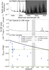 |
Fig. 1. (a) Night sky spectrum as a function of observed wavelength. The black line shows the night sky spectrum with an arbitrary normalization. The light gray and dark shaded areas indicate the wavelength range of the AO gap and the wavelength range that is not used in this work, respectively. (b) 5σ noise surface brightness (SB) for the typical parameters for optimized NBs (see Sect. 3.2) as a function of redshift (black line). The light gray shaded area indicates the redshift range of the AO gap. (c) M1500 as a function of z for the sample. The large filled blue stars, large open blue stars, and small open blue stars indicate our sources with ZCONF = 2, 3, ZCONF = 1, and ZCONF = 0, respectively. The black dots show nonisolated galaxies (see Sect. 2.2). The black and green lines represent the F775W apparent magnitude cut, and the criteria for the UV-bright sample, respectively. |
2.2. Catalog and sample selection
The MXDF catalog was constructed in two ways, a blind emission search in the MUSE cube (ORIGIN method) and spectra extraction with prior information (ODHIN method). The two types of information were merged into one catalog (Bacon et al., in prep.). Appendix A.1 gives a brief summary of the ORIGIN and ODHIN methods, the flow of the visual inspection, assignment of Rafelski et al. (2015)’s ID (RID), and the criteria of confidence levels (ZCONF) of spectroscopic redshifts (spec-z or zs). The MUSE sources that are included in the catalog of Inami et al. (2017) keep the same ID (MID) in the MXDF catalog. Most of the continuum-bright sources in Rafelski et al. (2015) are spectroscopically confirmed in the MXDF catalog. For instance, in the region with more than 100-h integration (r < 31 arcsec), 87% of HST/Advanced Camera for Surveys Wide Field Channel (ACS/WFC) F775W ≤ 27.5 sources have reliable spectroscopic redshifts, ZCONF = 2 or 3, and 7% have ZCONF = 1 redshifts. Moreover, 25 sources out of 26 F775W ≤ 27.5 galaxies, whose photometric redshifts (photo-z or zp) are within the targeted redshift range below, have ZCONF = 2 or 3 (see Fig. A.1). The spec-z for the remaining 1 source was assigned as explained below. We note that we used a preliminary version of the MXDF catalog (DR2 v0.8) in this study.
We targeted galaxies at z = 2.86 − 4.44 (excluding the Lyα redshift range in the AO gap) to investigate their Lyα haloes. There are two main reasons for this redshift range choice. First, at z ≤ 4.7 for Lyα (4700 − 7000 Å), the background noise level is stable compared to those at longer wavelengths (see the black shaded area indicating z ≥ 4.44 in Fig. 1a). The 5σ median SB noises for the typical parameters for the halo search (see Sect. 3.2) at z = 2.86 − 4.44 are shown in Fig. 1b. Second, at z ≤ 4.44, the HST band ACS/WFC F775W can capture the UV continuum of galaxies without being contaminated by Lyα emission (the same threshold as those used in Hashimoto et al. 2017; Kusakabe et al. 2020). In fact, McKinney et al. (2019) reported that some local galaxies show a wide Lyα absorption feature, which could extend to λ ≃ 1260 Å. These features were also confirmed at high redshifts (for stacked MUSE LAEs at z ≃ 2.9 − 4.6, Feltre et al. 2020). The threshold of z = 4.44 for rest-frame 1270 Å corresponds to 6900 Å, at which F775W filter has 3% transmission (see Sect. 4.3 in Matthee et al. 2021, for more details on the conservative choice of 1270 Å). In addition, we limited the field to the very deep area with 100- to 140-h integration (r < 31 arcsec) to have a homogeneous depth.
In order to build a spectroscopically complete sample, our parent sample is based on the HST catalog in Rafelski et al. (2015) with deep 5σ limiting magnitudes from 27.8 to 30.1 mag. The catalog is confirmed to be complete in UV at the redshift and M1500 ranges that we used in this paper (complete for M1500 ≤ −17 mag at z = 2.9 − 4.4, see Fig. 2 in Kusakabe et al. 2020). Out of a total of 9969 sources in the catalog, 797 sources are within the footprint of the more than 100-h integration region. Among them, 142 sources are brighter than 27.5 mag in F775W, which corresponds to a rest-frame UV band for sources at z = 2.86 − 4.44. This apparent magnitude cut is 0.5 mag fainter than that for the HST prior detection in the mosaic field in the MUSE-HUDF Survey in Inami et al. (2017). As mentioned above, 123 sources (87% of 142 F775W ≤ 27.5 sources) have a reliable spec-z from MUSE with ZCONF = 2 or 3, and 10 sources have a possible spec-z (ZCONF = 1). The remaining nine sources are not in the MXDF catalog as they do not show a clear feature in their spectra, but their continua are detected in the MXDF data cube (see below for more details).
Among the 123 ZCONF = 2 or 3 sources, 18 galaxies are located at z = 2.86 − 3.77 and z = 3.91 − 4.44, while 105 galaxies are outside the redshift range. Unfortunately, one galaxy, which is categorized as an LAE in the catalog of Inami et al. (2017) and shows UV lines in the MXDF data cube, has Lyα emission in the AO gap. Due to the limited spatial resolution of MUSE, RID = 7876 and 9944 were assigned to a unique MUSE source (MID = 103 at zs = 2.99). Such nonisolated sources were separately treated as described later.
Among the 10 ZCONF = 1 sources, nine sources have a possible spec-z at zs ≤ 2.86 (0.71, 1.10, 1.25, 1.67, 1.85, 1.91, 1.99, 2.34, and 2.67). Eight sources have a spec-z consistent with their photo-z in Rafelski et al. (2015), and one source with zs = 1.25 has a  (see Fig. A.1). All of them show clear continua at the blue edge of the MUSE spectra, implying that they should not be located at z ≥ 2.86. The remaining ZCONF = 1 source has zs = 3.94 (RID = 23135). It has ORIGIN-detected Lyα emission with a line flux signal-to-noise ratio (S/N) higher than 5 in the catalog (6.4). However, the Lyα center given by ORIGIN is spatially offset by
  from the position in Rafelski et al. (2015), and the spec-z does not match with
  . Moreover, the emission is close to the edge of the AO gap. We included the source in our parent sample, but it is not selected for a subsample with a UV absolute magnitude cut used to calculate the Lyα halo fractions, because of its faintness.
We inspected the MXDF data for nine sources that are not in the MXDF catalog. Seven sources of those nine sources at  ,
,  ,
,  ,
,  ,
,  ,
,  , and
, and  show clear continua at the blue edge of the MUSE spectra, which is not the case at z ≥ 2.86. One of the remaining two sources, RID = 54891, has
  and does not have an ORIGIN-detected emission line. However, it shows weak potential Lyα emission at z = 2.94 with a line flux S/N of 3.9. Because of the low S/N, the noisy spectrum, and the missmatch between zs and zp, it was not categorized as a ZCONF = 1 source and was not included in the MXDF catalog. To minimize a sample selection bias in this work, we assigned it a tentative spec-z of zs = 2.94. This object is not included in the UV-bright sample described later in this section. We confirmed that our main results can hold up with the subset. The other remaining source at z > 2.86 that is not in the MXDF catalog (RID = 6693) has
  and shows a break around 6250 Å in the MUSE spectrum, which can be interpreted as a Lyα break. The source has an emission line in the 1D spectrum, which could be interpreted as a Lyα emission line at z ≃ 4.17, but is contamination from a neighboring LAE. Then, we performed a cross correlation using the MARZ spec-z software (Hinton et al. 2016; Inami et al. 2017) on different spectra extracted from 1 to 5-pixel radius apertures and did not find realistic solutions. In order to obtain our best estimate of a tentative spec-z, we stacked the 1D spectra centered at wavelengths of different combinations of UV absorption lines among Si IIλ1260.42, O Iλ1302.17, Si IIλ1304.37, C IIλ1334.53, Si IVλλ1393.75, 1402.77, Si IIλ1526.71, C IVλλ1548.20, 1550.78, Fe IIλ1608.45, and Al IIIλ1670.79. It is challenging to determine a spec-z for faint sources at high redshifts with this method, but we note that we can get correct spec-z for brighter sources at z > 4 with ZCONF = 3, RID = 5479 and 7067. Although we did not find a significant absorption line at any redshift solution, zs = 4.167 shows 3 consecutive pixels with more than a 1σ dip compared to the continuum (1.2σ, 1.8σ, and 1.6σ) as a result of stacking of Si IIλ1260.42, C IIλ1334.53, and Si IVλ1393.75 lines. This is consistent with the interpretation of the Lyα break. We note that Si IVλ1402.77 at zs = 4.167 overlaps with a skyline. Therefore, we assigned a tentative spec-z, zs = 4.167. We did not discard these two objects (RID = 54891 and 6693) to minimize a selection bias. RID = 6693 can meet criteria for a UV-bright subsample described later in this section, while RID = 54891 does not, which means that it does not affect our main conclusion. We took into account the effect of uncertainties in the spec-z estimation (see Sect. 3.4.1).
In total, we have 21 galaxies at z = 2.86 − 3.77 and z = 3.91 − 4.44 with F775W ≤ 27.5 mag as the parent sample listed in Table 1. An overview of the 21 sources is given in Figs. 2–5 (see Fig. 2 for enlarged panels for two sources as examples). We calculated the rest-frame UV magnitude (M1500) and the UV slope (β) using zs, F775W, F850LP, and F105W in the same manner as in Kusakabe et al. (2020). The M1500 ranges from −19.9 to −18.1 with an average value of −18.9, which is fainter than M* at z ≃ 3.7, −20.88 mag (Bouwens et al. 2015). The average M1500 corresponds to a typical dark matter halo mass of Mh ≃ 1 × 10¹¹ − 2 × 10¹¹ M⊙, which is estimated from a M1500 − Mh relation from the GALICS semi-analytic model in Garel et al. (2015). The UV slopes range from −2.3 to 0.2, with an average value of −1.6. The distribution of M1500 and zs of the sample is shown in Fig. 1c. Out of the 21 galaxies, six galaxies, RID = 7067, 7901, 9814, 9863, 10018, and 23124 (MID = 7091, 180, 149, 106, 6700, and 7073) were included in the Lyα-selected sample for the previous MUSE-LAH study in the HUDF, and all of them are confirmed to be LAHs (Leclercq et al. 2017). Among the 15 new sources, five galaxies, RID = 5479, 7876, 22230, 23408, and 23839 (MID = 7089, 103, 163, 174, and 118), are included in the MUSE-HUDF catalog in Inami et al. (2017) as well as in the updated version in Bacon et al. (in prep.), but they were not selected in the sample in Leclercq et al. (2017), due to their low ZCONF values (≤1), low S/N values of Lyα (< 6), or close neighboring objects. In order to validate that our sample is not biased s the LAE selection, we checked LAE fractions (XLAE) for our sample following Kusakabe et al. (2020). Rest-frame equivalent widths of Lyα emission (EW(Lyα)) were calculated with Lyα fluxes at the galaxy’s stellar-component scale (see Appendix A.3 for a description of EW measurements and XLAE calculations). With EW(Lyα)≥20 Å, which is a common criterion of LAEs, the XLAE for our entire sample (−20 ≤ M1500 ≤ −18.0, z = 2.9 − 4.4) is  . For a fair comparison, we also calculated the XLAE with EW(Lyα)≥65 Å for our entire sample as
  , which is similar to
  ,
,  , and
, and  for EW(Lyα)≥65 Å and −21.75 ≤ M1500 ≤ −17.75 at z = 3.3, 4.1, and 4.7, respectively, in Kusakabe et al. (2020). It suggests that our sample is unbiased. The small difference in the XLAE between the two samples could be explained by the cosmic variance due to our small survey volume in the MXDF (4 × 10³ cMpc3).
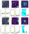 |
Fig. 2. Examples of the overview with two sources (a LAH RID = 4764 and a non-LAH RID = 5479). The first two rows show RID = 4764, while the last two rows show RID = 5479. (a) HST F775W image (rest-frame UV). The Rafelski’s ID (RID), the MUSE ID (MID), zs, ZCONF, and M1500 are indicated. The smaller and larger cyan circles present rin and rCoG (Sects. 3.1 and 3.2). (b) MUSE broad band image summed over the rest-frame UV range 1300–1800 Å. The image is smoothed with a 2D Gaussian filter with a standard deviation of 1 pixel. Spectroscopic redshifts of sources in the MXDF catalog in the minicube are indicated. (c) Optimized narrow band for Lyα with the neighboring object mask (purple areas). The image is smoothed with a 2D Gaussian filter with a standard deviation of 1 pixel. The white contours indicate a SB of 2 × 10⁻¹⁹ erg s−1 cm−2 arcsec−2. (d) 1D spectrum around the wavelength of Lyα extracted inside the target’s continuum-component mask. The spectra and the 1σ uncertainty are represented by the black line and the gray shaded area, respectively. The spectral width of the flux-maximized NB and the wavelength of Lyα converted from zs in the MXDF catalog are shown by the cyan dashed and solid lines, respectively. The spectral slices used to produce the optimized NB are indicated by the yellow shaded areas for sources with high S/N spectral slices at r = rin − rCoG. (e) 1D spectrum around the wavelength of Lyα extracted in r = rin − rCoG. (f) Radial SB profile of Lyα emission in log scale measured on the optimized NB image. The cyan shaded areas represent the radial range, r = rin − rCoG (see Sect. 3.3). The panel shows whether the source is an isolated or nonisolated object, and whether it is a Lyα halo (LAH) or non-LAH. All images are 15 arcsec each on a side. We note that the segmentation maps and the masks as well as zoomed-in HST F775W cutouts (4″ × 4″) are shown in Figs. C.1 and C.2. |
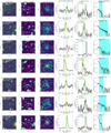 |
Fig. 3. Overview of the first 7 sources in order of RID except for RID = 4764 and 5479. Each row shows a different object. Panels a–f: are the same as those of Fig. 2. Panel a: MID = 0 means that no MUSE ID is assigned in the MXDF catalog (i.e., ZCONF = 0). Panels d and e: the spectral slices used to produce the optimized NB are indicated by the yellow and orange shaded areas for sources with high S/N spectral slices at r = rin − rCoG and those with low S/N spectral slices at r = rin − rCoG, respectively (see Sect. 3.2). We note that the emission ring shown in the NB of RID = 7876 is caused by the mask for a source with extended emission. Since the ring is located outside rCoG, it does not affect our results. |
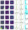 |
Fig. 4. Same as Fig. 2, but for the middle 6 sources in order of RID. Each row shows a different object. Panels a–f: are the same as those of Fig. 2. We note that the emission rings shown in the NB of RID = 9944 is caused by the mask for a source with extended emission. Although the ring feature of RID = 9944 overlaps with r = rin − rCoG, this object is not included in the isolated sample (as well as RID = 7876), and the main conclusion about the Lyα halo fraction is not affected by the ring. |
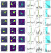 |
Fig. 5. Same as Fig. 2, but for the last 6 sources in order of RID. Each row shows a different object. Panels a–f: are the same as those of Fig. 2. |
Overview of the galaxy sample.
As in the case of RID = 7876 and 9944 (MID = 103), the MUSE spatial and spectral resolutions are not always high enough to disentangle the spec-z assignment. It can also make it difficult to assign extended Lyα emission to close HST sources. Following Inami et al. (2017), we checked if galaxies have close projected neighbors within  using the catalog of Rafelski et al. (2015). We did not consider MUSE LAEs as neighbors here, because extended Lyα emission from satellites is one of the candidates for the powering sources of Lyα haloes. In our sample, 6 sources (RID = 4764, 4838, 5479, 7876, 9944, and 10018) have one HST-detected galaxy within
  . We used the MXDF catalog to check the spec-z of the HST neighbors. The HST neighbors of RID = 4764 and 10018 are located at different redshifts and do not contaminate the Lyα NB used in the halo tests (RID = 10516 at zs = 1.42 and RID = 10046 at zs = 2.59, respectively). Unfortunately, the HST neighbor of RID = 5479, RID = 5498, does not have a spec-z, but the photo-z,
  , is not close to the spec-z of RID = 5479, zs = 4.16. Therefore, we regarded these three sources as isolated sources. Meanwhile, the HST neighbor of RID = 4838 (RID = 6666 at zs = 3.06) has a velocity offset of ΔV = −25.4 km s−1 from RID = 4838, which indeed contaminates the Lyα NB used in the halo test (see Figs. 3 and A.3). They belong to a group of galaxies within the cosmic web detected with Lyα emission in Bacon et al. (2021), see Appendix A.4 for more details. Since both RID = 7876 and 9944 are assigned to counterparts of MID = 103 at zs = 2.09, they are interpreted to share Lyα emission in their Lyα NBs. In addition, MID = 103 has another neighbor within
  , RID = 7847 at zs = 3.00 in our sample (ΔV = 458 km s−1 from RID = 7876 and 9944), which leads to mutual contamination of their Lyα NBs (see Figs. 3 and 4). Although RID = 7847 is located further than
  from the positions of RID = 7876 and 9944, these three sources also belong to a larger structure of cosmic web found in Bacon et al. (2021), as shown in Fig. A.4. Therefore, RID = 4838, 7847, 7876, and 9944 might live in a different kind of environment from the rest of our sample, which may affect the existence of a Lyα halo and Lyα halo properties. Additional details of four nonisolated sources are given in Appendix A.4. We calculated Lyα halo fractions for the isolated sources and the nonisolated sources as well as all sources in Sect. 3.4.
In Fig. 1c, we introduce an unbiased subsample, the “UV-bright sample”, with a redshift range of z = 2.86 − 4.44 with −20.0 ≤ M1500 ≤ −18.7 mag. It contains 12 galaxies, of which 10 are isolated sources and two are nonisolated galaxies.
In summary, our sample was built in two steps. First, we selected galaxies brighter than F775W = 27.5 in the catalog of Rafelski et al. (2015), which corresponds to rest-UV for galaxies at z ∼ 3 − 4. Second, we applied a selection on the spectroscopic redshift of these objects to keep only galaxies with z = 2.86 − 4.44. We note that all galaxies except nine have a spectroscopic redshift from the MUSE catalog. These nine galaxies have a photometric redshift and their continuum is detected in the MUSE cube. Seven of them have zp = 0 − 2.5 with clear continuum detection at the blue edge of the MUSE cube: there is no sign of a Lyman break, which is very unlikely for sources at z > 2.86. We did not include these sources in our sample. The remaining two sources were included in our sample, with ZCONF = 0, in order to minimize a possible selection bias in favor of Lyα emitters. Therefore, we stress that our sample of 21 galaxies is rest-UV selected.
2.3. Continuum subtraction
For the following analysis, we provided  cutouts of the MUSE cube (minicube), the HST/ACS/WFC F775W image (Beckwith & Stiavelli 2006; Illingworth et al. 2013) and the HST segmentation map (Rafelski et al. 2015) for each source. We used continuum-subtracted minicubes for most of the analysis in this paper, such as the Lyα narrow bands explained in Sect. 3.
The continuum subtraction is useful not only to investigate line emission, but also to remove neighboring sources around a targeted source. The continuum minicubes were provided from a spectral median filtering on the original minicubes in a 100-pixel spectral window (±50 pixels) in a similar manner to those in previous MUSE papers (with a 200-pixel window, e.g., Leclercq et al. 2017, see also Herenz et al. 2017 for a 150-pixel window) and in addition excluded ±400 km s−1 around the Lyα wavelength. Although the method with a 200-pixel window was validated for the MUSE-HUDF and MUSE Wide data sets, in particular for LAEs, it can overestimate the continuum around a Lyα break (Lyα absorption) for UV-bright galaxies in the MXDF, since the MXDF data are deep enough to detect the UV continuum and the break. The oversubtraction due to the general 200-pixel window leads to artificial absorption at the position of a targeted UV source on a Lyα narrow-band image for some sources. We examined different settings for the continuum minicubes: (1) the general setting with a 200-pixel window, (2) a 200-pixel window with a mask around the Lyα wavelength (±400 km s−1), (3) a 100-pixel window with a mask around the Lyα wavelength, and (4) a 60-pixel window with a mask around the Lyα wavelength. The Lyα masks cover 10 to 14 spectral slices at z = 3 to 4.4, respectively.
We found a trend that the continua around Lyα were increasingly overestimated from settings (4) to (1) (see Fig. B.1). This trend becomes stronger for galaxies showing a Lyα absorption feature. We also found that the 60-pixel window was too narrow to derive an accurate continuum. We confirmed that the continuum at λ > 1270 Å in the rest frame did not change among the four settings. Therefore, we adopted the third setting with a 100-pixel window, with a mask around Lyα. In Appendix B, we discuss two examples of the difference in the radial SB profiles for four different settings as described below (see Fig. B.1).
The obtained continuum minicube was subtracted from the original minicube to provide the continuum-subtracted minicube. Even with this optimized choice, we have a potential uncertainty in the continuum estimation around the Lyα wavelength at the position of a targeted UV-selected source, which however does not affect the extended Lyα emission beyond the galaxy’s stellar component. For this reason, we did not use the spatial pixels on the main part of the galaxy’s stellar component when we tested for the existence of Lyα haloes in the third step (see Fig. 6).
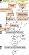 |
Fig. 6. Flowchart of the main part of our analysis with the four steps. The input data are indicated by the yellow rounded boxes at the top of the panel, while output data are indicated by the orange rounded boxes. The analysis and classification are shown by rectangles and diamonds, respectively. The obtained samples and parameters are presented by circles. The details of each step are provided in Sects. 2.3, 3.1–3.4. The numbers colored blue indicate the sections as a reference. The flux-maximized NBs were used to obtain the average SB profiles in Sect. 4.2.1. |
3. Lyα haloes around UV-selected galaxies
The main part of our analysis consists of four steps. First, we created a mask for the continuum-like component (target’s continuum-component mask) and a neighboring object mask for neighbors for each source (Sect. 3.1). The target’s continuum-component mask was used to obtain an inner radius. Second, we provided a flux-maximized Lyα NB with a curve-of-growth radius by tuning the width of the NB and the radius to maximize the halo flux and then provided optimized NBs only with high-S/N spectral slices (Sect. 3.2). Third, we tested for the existence of a Lyα halo around each source (Sect. 3.3). Fourth, we derived the Lyα halo fractions (Sect. 3.4). The flow of the analysis is illustrated in Fig. 6.
3.1. Masks and inner radii
We used a target’s continuum-component mask to extract the 1D spectrum within the galaxy’s stellar-component scale and to define the inner radius used to adjust the Lyα NB (Sect. 3.2). The continuum-component masks were created with the HST segmentation maps in a similar manner to those used to create object masks for HST prior extractions in Inami et al. (2017). The HST segmentation map indicates areas in which galaxies are detected and defines the boundaries of the objects (more details are given in Appendix C, see also Figs. C.1 and C.2). If a pixel does not belong to the target on the cutout segmentation map, we replaced the corresponding pixel of the F775W cutout with zero and provided an HST target image. We convolved the HST target image with the MUSE PSF at the Lyα wavelength. Then, we resampled the PSF-convolved HST target image with the spatial resolution of MUSE, aligning it with the MUSE sky coordinate. We normalized the PSF-convolved image so that the peak became 1. To provide the target’s continuum-component mask for each source, we applied a threshold value of 0.2 to the normalized convolved image (see Figs. C.1 and C.2). This threshold was used to extract the spectra from non-AO MUSE cubes for the HST-prior sources in the catalog in Inami et al. (2017). For the MXDF data, the target’s continuum-component masks typically include 66% of the total fluxes in the target’s continuum-component images. We defined an inner radius, rin, beyond which the normalized PSF-convolved profile is below 0.2. We used rin in the SB profile measurements for the Lyα halo tests later, to exclude the SB inside the galaxy’s stellar-component scale. The rin ranges from 0.8 arcsec to 1.0 arcsec with an average value of 0.81 arcsec (in physical scales at different redshifts, 5.5 to 7.0 kpc with an average of 6.2 kpc).
We used a neighboring object mask to exclude pixels that might be affected by bright neighbors on a MUSE NB when we adjusted the Lyα NB and measured the Lyα radial SB profile. To mask the bright-continuum emission from the neighbors, we created a broad band (BB) image from the original MUSE minicube without continuum subtraction at rest-frame 1300 to 1800 Å for the target (see Figs. 2–5). Then we clipped pixels whose S/N are higher than 20. With this threshold, we can mask the main part of continuum-bright galaxies on the optimized NBs and the flux-maximized NBs. A lower S/N threshold for the BBs, 10, changed the S/N values for extended Lyα emission on the optimized Lyα NBs used in the halo tests (see Sect. 3.3.1) because we lost the area with Lyα emission. However, it did not change the results for the tests for haloes for any sources, except for one (RID = 23408). Since we used continuum-subtracted minicubes for most of the analysis and would like to keep as many spatial pixels as possible, the higher threshold of 20 was adopted. The two masks for each source are shown in Figs. C.1 and C.2. We note that the emission rings showing up at the left bottom of the NBs of RID = 7876 and 9944 in Figs. 3 and 4 are caused by a source whose emission extends beyond the neighboring-object masks. The main conclusion about the Lyα halo fraction is not affected by the ring features, since the objects are not included in the isolated sample.
3.2. 3D curve-of-growth for narrow bands
To define a 3D volume in a minicube that includes all the potential flux of a Lyα halo, we adjusted the NB width and the annulus used for the halo photometry simultaneously, using the spec-z and the spatial coordinate of the HST targets. The inner radius of the annulus is rin. The outer radius of the annulus is a curve-of-growth radius (CoG; rCoG), which is commonly used to derive the total Lyα flux from a NB image (e.g., Drake et al. 2017; Leclercq et al. 2017). It is the minimum radius among consecutive 1 pix-width annuli with increasing radius around a target, whose flux reaches or dips below zero (see Drake et al. 2017, for more details).
First, we created 400 NBs from a minicube with a combination of widths to redder and bluer wavelengths from 0 to 20 adjacent pixels around the Lyα wavelength. We applied the 2D neighboring object mask to the created NBs. Then, we derived rCoG by annulus photometry with PHOTUTILS (Bradley et al. 2021) on each NB and measured the flux between rin and rCoG centered at the spatial coordinate of the HST target. Finally, we chose the combination of a NB width and rCoG that gives the highest rin − rCoG flux. The flux-maximized NB widths range from 21.25 Å to 48.75 Å (4.1 Å to 12.2 Å, or 1014.9 km s−1 to 3012.1 km s−1) with the average of 31.8 Å (7.5 Å, or 1848.0 km s−1) in observed wavelength (rest-frame wavelength or velocity difference). The rCoG ranges from 1.4 arcsec to 7.2 arcsec (10.5 to 56.8 kpc) with the average of 4.2 arcsec (32.0 kpc). The rCoG and NB width are shown in Figs. 2 and 3. The rCoG and the flux-maximized NB were used to measure a surface brightness profile in the third step and in Sect. 4.2.1, respectively.
We optimized the Lyα NBs by selecting spectral slices with S/N > 1.5 for the flux between rin and rCoG. We inspected the spectral slices visually and discarded the pixels whose signals might be enhanced by noise peaks. Out of 21, 18 sources have at least five spectral slices (6.25 Å) with S/N > 1.5. The total wavelength width ranges from 8.75 Å up to 22.5 Å, with an average value of 14.5 Å in the observed frame (corresponding to 539.7 km s−1 to 1298.2 km s−1, and an average of 838.5 km s−1). The remaining three sources (RID = 6693, 23135, and 54891) do not have a sufficient number of high S/N pixels. In particular, RID = 23135 and 54891 do not show a realistic line profile. Their pixels with S/N > 1.5 seem to be affected by noise. Therefore, we created the optimized NBs for these sources using the 1D spectra inside the target’s continuum-component mask. RID = 23135 has six S/N > 1.5 spectral slices, which were used to create the optimized NB. However, RID = 6693 and 54891 have only four and two S/N > 1.5 spectral slices, and the optimized NB was created from the five highest-S/N spectral slices. The chosen spectral slices are shown by yellow or orange shaded areas on the spectra in Figs. 2–5. With the average width of optimized NB and the average unmasked area between rin and rCoG, the median 5σ SB limit is estimated to be 4.1 × 10⁻¹⁹ erg s−1 cm−2 arcsec−2 over the redshift range (see Fig. 1b), and the 5σ flux limit is 3.1 × 10⁻¹⁸ erg s−1 cm−2 over the redshift range. The optimized NB were used to measure a surface brightness profile in the third step.
3.3. Test for the presence of Lyα haloes
We tested for the existence of Lyα haloes with two steps. First, we checked the S/N of fluxes in the annulus from rin to rCoG to select LAH candidates (Sect. 3.3.1). Second, we tested for the existence of Lyα haloes with the radial SB profiles at r = rin − rCoG (Sect. 3.3.2), the results of which are described in Sect. 3.3.3. We investigated non-LAH objects in Sect. 3.3.4 and Appendix D with completeness simulations of the halo tests.
3.3.1. Selection of LAH candidates based on the S/N at r = rin − rCoG
We measured the S/N of fluxes in the annulus from rin to rCoG, S/N(rin − rCoG), on the optimized NBs using PHOTUTILS with the two masks. The sources that have a S/N higher than or equal to three were regarded as Lyα halo candidates, which were also visually inspected. The top panel of Fig. 7 shows the histogram of S/N(rin − rCoG). Among 21 galaxies, 19 are LAH candidates. The two objects with low S/N values are RID = 23135 and 54891, whose NBs were optimized based on the 1D spectra at r ≤ rin in Sect. 3.2. They have low S/Ns on the 1D spectra at r = rin − rCoG, and the low values of S/N(rin − rCoG) on 2D NBs were expected.
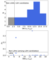 |
Fig. 7. Results of the tests for the existence of a Lyα halo. Top panel: histogram of the flux S/Ns between r = rin and rCoG measured on the optimized Lyα NBs. Blue and gray histograms indicate galaxies above and below the threshold of S/N = 3 (black dashed line), Non-LAHs and LAH candidates, respectively. RID = 23135 has a negative S/N(rin − rCoG) and is counted as S/N(rin − rCoG) = 0 in the plot. Bottom panel: probability of the null hypothesis that the SB profile at r = rin − rCoG matches that of the target’s continuum-component profile vs. flux S/N between r = rin and rCoG for the LAH candidates. A black dashed line represents the border of LAHs and Non-LAHs. |
3.3.2. Test with Lyα radial SB profiles
In order to confirm the presence of extended Lyα emission, we checked if the emission is not from the outer wing of bright central Lyα emission. To do so, we assessed the null hypothesis that the source does not have Lyα emission more extended than the PSF-convolved continuum-like component. In other words, we measured the significance of the deviation of the observed radial SB profiles from those of the target’s continuum-component images provided in Sect. 3.1 (p0 test). Our method carefully prevents potential uncertainties of SB profiles at r < rin due to the continuum subtraction. We measured the observed SB profile on the optimized NB using PHOTUTILS with two masks. The default width of the radial bins was one MUSE spatial pixel, but the bins were combined with the outer bins to have S/N ≥ 2. If spatial pixels at large radii close to rCoG had too low S/Ns, which reduced the combined S/N and made it lower than two, we did not use the pixels in the fitting. We note that it did not change the results of the halo test for the sample but gives lower p0 values (higher reduced χ2), which helps detect diffuse haloes combined with other conditions. We measured the effective area considering the masks and derived the SB profiles by dividing the fluxes with the effective area. Then, we fit the observed SB profile with that of the target’s continuum-component in the range of rin to rCoG and measured the reduced χ2, which was converted into the probability of the null hypothesis, p0, with scipy.stats.chi2.sf. Here, the number of degrees of freedom (d.o.f.) is 1 smaller than the number of the combined radial bins. The free parameter is the amplitude of the SB (i.e., flux). If a source has a Lyα halo, the SB profile from rin to rCoG is significantly different from that of the target’s continuum-component, which makes p0 small. Our threshold for the probability of the null hypothesis,  , is 0.05, which is the same as that used in Leclercq et al. (2017).
We visually investigated the sources that have a larger reduced χ2 than the threshold (see Table 2). We note that the results of the null hypothesis tests were the same if we used different thresholds of S/N for the radial binning, 1.0, 1.5, and 2.0, and when we adopted different  from 0.04 to 0.1. We also checked the results for the four different settings in the continuum subtraction. The results were the same for all the sources except for one object (RID = 23408). These checks imply that our tests for the existence of Lyα haloes are robust. The results of the tests are described in Sect. 3.3.3 (see also Table 2 and Figs. 7 and 8).
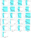 |
Fig. 8. SB profiles from the optimized NBs with results of the Lyα halo tests. The gray, black, and blue points indicate the observed radial profiles, those used for the fit (with binning if needed), and the best-fit SB profiles of the PSF-convolved continuum-like component, respectively. The x error bars of the black points mark the range for each (combined) radial bin. The cyan shaded areas represent the radial ranges, r = rin − rCoG (see Sect. 3.3). The classification of LAH or non-LAH, the S/N of the flux at r = rin − rCoG, and the probability of the null hypothesis that the SB profile at r = rin − rCoG matches that of the target’s continuum-component profile are shown at the top of each panel. |
Summary of the tests for the existence of Lyα haloes.
With this test, we could miss very faint or diffuse Lyα haloes below the detection limits and Lyα haloes whose shapes are very different from our circular assumption (see Sect. 3.3.4 for more details). The S/N ≥ 3 criterion corresponds to SB ≥ 3.2 × 10⁻¹⁹ erg s−1 cm−2 arcsec−2 and flux ≥ 2.2 × 10⁻¹⁸ erg s−1 cm−2, in the case of the average width of the optimized NB and the average unmasked area between rin and rCoG (see Sect. 3.2 and Fig. 1b).
As a final note, our method is different from Leclercq et al. (2017). Their method was designed for galaxies with strong central Lyα emission which can de facto always be fit by the same exponential profile as the continuum. Our galaxies are UV-selected and do not always show strong central Lyα emission. In practice, their inner Lyα emission is not well modeled by the continuum so that the method of Leclercq et al. (2017) is not applicable to our sample. The higher signal-to-noise ratio of our data also makes their modeling assumptions more difficult in practice in our sample. We thus use a more general method, which we verified recovers the LAHs of Leclercq et al. (2017) for the six objects we have in common (and which thus all have strong central Lyα emission).
3.3.3. Results of the halo test
Among the 19 LAH candidates, 17 Lyα haloes around the galaxies are confirmed with p0 ≤ 0.05 (see the bottom panel of Fig. 7). All LAH sources have small p0 values, ranging from 3.0 × 10−68 to 0.035 (corresponding to reduced χ2 values from 28.5 to 2.6), which indicate significant deviations of the radial SB profiles from those of the PSF-convolved continuum-component profiles at r ≥ rin. However, the remaining two sources, RID = 5479 and 22230, are not confirmed to have a Lyα halo due to their high p0 values, 0.37 and 0.27, respectively, which are higher than the thresholds. Interestingly, both sources have bright Lyα fluxes and high S/N(rin − rCoG) values, but the radial SB profiles at r ≥ rin are statistically consistent with those of the target’s continuum-component images (see Sect. 3.3.4 and Appendix D.2). The radial SB profiles and the results of the tests for individual sources are summarized in Fig. 8 and Table 2.
In total, we have 17 LAHs and four non-LAHs. The results of this LAH test are consistent with those in Leclercq et al. (2017) for the six common sources with RID = 7067, 7901, 9814, 9863, 10018, and 23124, which are classified as LAHs in both studies, though the methods used are different. Interestingly, we found LAHs around non-LAEs with net negative EW(Lyα): for instance, RID = 4587 and 4764, which have EW(Lyα)net ≤ −10.0 Å and −14.2 Å, respectively, as demonstrated in Appendix A.3 and Fig. A.2 (see also the central dip on the SB profiles in Fig. 8). RID = 7876 and 9944 might be also non-LAEs with LAHs. However, unfortunately, they are nonisolated sources, and we cannot decline a possibility that their LAHs are mainly contributed from other sources in the large-scale structure like RID = 7847 (see Fig. A.4). This is the first time to confirm the presence of LAHs around non-LAEs. Further discussion of the Lyα line properties and galaxy populations is beyond the scope of this paper but it could be interesting to investigate in the future.
3.3.4. Non-LAH objects
Faint diffuse Lyα haloes could be undetected because they would be hidden in the noise. We investigated the four non-LAH objects and simulated their completeness individually. Here we briefly explain the simulations, introduce non-LAHs, and comment on a non-LAH included in the UV-bright sample (Sect. 2.2). The details of the simulations and the remaining three non-LAHs are described in Appendix D.
The completeness of our halo test is sensitive to the SB profiles of haloes. Assuming an exponential SB profile, as used in Wisotzki et al. (2016) and Leclercq et al. (2017), we applied the same halo test to mock NBs of noise and PSF-convolved halo models (see Appendix D for more details). We also simulated haloes with a Lyα continuum-like component, whose flux was matched to the central Lyα flux of the observed non-LAH objects. Figure 9 summarizes the parameter sets with a 50% completeness of the four non-LAHs for both cases. Generally, the completeness decreases when the central surface brightness Ih decreases or the scale length for haloes rs, h decreases. The profiles are similar among the four sources but depend on the noise levels. If a galaxy has a bright Lyα continuum-like component, the completeness can be enhanced or suppressed depending on the parameters (see Fig. D.3). The completeness for individual sources is shown in Figs. D.1 and D.2, and our halo tests are found to be complete when the halo fluxes are equal to or brighter than ≃4 × 10⁻¹⁸ erg s−1 cm−2 to 6 × 10⁻¹⁸ erg s−1 cm−2 in most of the parameter ranges. We checked the parameters measured in Leclercq et al. (2017) for the six common sources with Lyα haloes. These sources are mostly located above the 50% completeness lines for non-LAH sources.
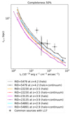 |
Fig. 9. Halo parameter set (Ih and rs, h) showing 50% completeness for four non-LAH objects. We explored potential halo parameters for four non-LAHs by simulating completeness values of the halo tests. We assumed exponential profiles for the halo and continuum-like component models (h + c) shown by dashed lines and for halo only models (h) shown by solid lines (see Appendix D). The gray solid (black dashed), orange solid (red dashed), magenta solid (violet dashed), and cyan solid (blue dashed) lines represent RID = 5479, RID = 22230, RID = 23135, and RID = 54891 with halo only models (halo and continuum models), respectively. The black crosses indicate the halo parameters measured in Leclercq et al. (2017) for the common sources between Leclercq et al. (2017) and ours. |
Out of the four non-LAHs, one object has a high S/N(rin − rCoG) (> 10), but no extended emission is significantly confirmed (RID = 5479). Another object with S/N(rin − rCoG) = 6.7 has anisotropic spatially offset Lyα emission (RID = 22230). Its extended emission cannot be confirmed with the current method and data set. The remaining two objects do not have detectable emission at r ≥ rin. The last three objects are not included in the UV bright sample, and therefore the results of the halo tests for the last three sources do not affect the main conclusions of this paper.
RID = 5479 has a high confidence level of ZCONF = 3 for zs = 4.16 in the MXDF catalog and is UV bright, M1500 = −19.34. It clearly shows Lyα emission lines on the 1D spectra for both r ≤ rin and r = rin − rCoG as shown in Fig. 3, with rin = 1″ and  . The S/N(rin − rCoG) is 12.94. However, the radial SB profile at r ≥ rin follows that of the MUSE PSF-convolved HST profile (continuum-like component), and the p0 value is as high as 0.38 (see Fig. 7). The radial SB profiles are also consistent at r ≤ rin. According to the completeness simulations, the completeness is approximately 50%, for instance, when the parameters are rs, h = 5.5 kpc and Ih = 8.8 × 10⁻¹⁹ erg s−1 cm−2 arcsec−2 or rs, h = 10.3 kpc and Ih = 2.4 × 10⁻¹⁹ erg s−1 cm−2 arcsec−2 (see Fig. D.1). As discussed in Appendix D, the completeness can be lowered when a source has a bright continuum-like Lyα component at the center, which can hide a halo feature. However, this only happens in a narrow parameter range, and the bright continuum-like Lyα component can also enhance the completeness for some cases (Fig. D.3). We conclude that it does not constitute a serious bias in our tests. From the distribution of the median rCoG in the simulations, we also find that the measured rCoG prefers the halo parameters with completeness values lower than 50%. The limitation of our data and method for the halo detection for RID = 5479 is illustrated in Fig. D.1.
If deeper IFU data with a higher spatial resolution than the MXDF data were available, it could be possible to detect faint and compact Lyα haloes among them. However, we would like to recall that our MUSE data were taken with AO and have an unprecedented depth of 100 to 140-h integration, the longest exposure times on the VLT so far. Considering the small sample size and the small number of non-LAHs, we did not correct for the incompleteness below.
3.4. Lyα halo fraction
3.4.1. Calculation of the Lyα halo fraction and its uncertainties
The fraction of Lyα haloes around UV-selected galaxies, XLAH, is defined as follows:
 (1)
(1)
where NLAH, NNon-LAH, and NUV are the number of objects in a LAH sample, a non-LAH sample, and a parent sample, respectively. We calculated XLAH for isolated sources and nonisolated sources separately, and for both subsets, for the UV-bright sample and the whole sample.
We calculated the statistical uncertainty in XLAH. Statistical uncertainties for fractions (i.e., Bernoulli trials) are given by a binomial proportion confidence interval (BPCI). Following our previous paper on LAE fractions (Kusakabe et al. 2020), we derived the statistical uncertainties in XLAH using astropy.stats.binom_conf_interval, with the Wilson score interval as an approximation formula (Wilson 1927). Our 1σ uncertainties correspond to 68.3% confidence intervals. For samples including RID = 6693 or 54891, which has a low ZCONF = 0, we adopted fractions including them in the Lyα fractions but took conservative uncertainties consisting of the minimum and maximum values of 68.3% confidence intervals of fractions with and without RID = 6693 or 54891.
There are three other potential contributions to the uncertainty in XLAH. The first are the uncertainties in NLAH due to the incompleteness of Lyα halo confirmations. As discussed in Sect. 3.3.4, the completeness of haloes sensitively depends on the halo SB profiles. Although spatial and spectral profiles of individual Lyα haloes around LAEs have been investigated (e.g., Leclercq et al. 2017, 2020; Claeyssens et al. 2019), we do not know the true distribution of the parameters of the halo profiles below the detection limits. Therefore, we did not correct for a completeness factor for NLAH in this study. The number of non-LAHs is small for our samples and the completeness correction would thus not change our main conclusions. The second contribution comes from the uncertainty in the PSF estimation for the MXDF (Bacon et al., in prep.). Since the survey area of the MXDF is not large, and the MXDF data cubes were obtained by stacking many different observations, the PSF is smoothed and homogenized. Therefore, the uniform formula for the PSF applied to the entire field should not have a significant effect on our Lyα halo tests. Third, we have the field-to-field variance. Since the survey volume of MXDF is limited to 4.0 × 10³ cMpc3 (z = 2.86 − 4.44, excluding the AO gap), our measurement of XLAH may be different from the cosmic average. There is a possibility that XLAH depends on the environment. Therefore, we calculated XLAH for both the sample of all the sources and of isolated sources as precisely as possible.
3.4.2. High Lyα halo fractions
Figure 10 shows a high Lyα halo fraction for the sample including all sources,  % (the dark gray bar in the first column). We note that all the non-LAHs are categorized as isolated galaxies (Sect. 2.2). However, the fraction remains high even when the sample is limited to the 17 isolated sources,
  %. The XLAH increases to
  % for nonisolated galaxies, though it is consistent within the 1σ error bars. Since all the sources were selected from the apparent magnitude cut of F775W, we also check XLAH for the UV-bright sample with −20.0 ≤ M1500 ≤ −18.7. The Lyα halo fraction is as high as
  % (the green bar in the first column). Even when we split them into isolated galaxies and nonisolated galaxies, the XLAH values remain high,
  % and
% and  %, respectively. The numerical values of LAH fractions are listed in Table 3.
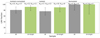 |
Fig. 10. Lyα halo fractions for the complete sample (gray bars) and the UV-bright sample (−20.0 ≤ M1500 ≤ −18.7; green bars). The XLAH for isolated sources and that for nonisolated sources are shown in the second and third columns, respectively. The black error bars indicate 68.3% confidence intervals. |
Lyα halo fractions for all the sources and the UV-bright sample.
The detection of extended Lyα emission with stacked Lyα narrow bands for the UV-bright galaxies cannot provide information on the individual presence of a Lyα halo (e.g., Steidel et al. 2011). The general presence of Lyα haloes is confirmed for individual UV-selected galaxies with observations for the first time in this work. It is similar to the high fraction of Lyα haloes around high-z MUSE LAEs (e.g., about 80% in Leclercq et al. 2017; Saust et al., in prep.), though the methods are different. We discuss the cause of the high Lyα halo fractions in the next section.
4. Discussion
We discuss implications from the high Lyα halo fractions, incidence rates of Lyα emission, and implications from four non-LAHs in Sects. 4.1–4.3, respectively.
4.1. Why do most of galaxies have a LAH?
It is now well established that there is extended Lyα emission around individual LAEs (Wisotzki et al. 2016; Leclercq et al. 2017). The key result of the present study is that not only LAEs have Lyα haloes: we found a very high Lyα halo fraction of ≃80 − 90% for our UV-selected galaxies at z = 2.9 − 4.4, in other words, star-forming galaxies at high redshifts. It implies that UV-selected galaxies generally have a significant amount of cool/warm gas in the CGM.
As introduced in Sect. 1, various mechanisms have been proposed to power Lyα haloes: (1) scattering of Lyα from star-forming regions (e.g., Laursen & Sommer-Larsen 2007; Zheng et al. 2011), (2) gravitational cooling radiation (e.g., Haiman et al. 2000; Fardal et al. 2001), (3) star formation in satellite galaxies (e.g., Zheng et al. 2011; Mas-Ribas et al. 2017a,b; Mitchell et al. 2021), and (4) fluorescence (e.g., Furlanetto et al. 2005; Cantalupo et al. 2005; Kollmeier et al. 2010; Mas-Ribas & Dijkstra 2016; Mas-Ribas et al. 2017b). In process (1), Lyα photons are produced in star-forming regions inside galaxies and then scattered by H I gas in the ISM and the CGM (e.g., Barnes & Haehnelt 2010; Dijkstra & Kramer 2012; Verhamme et al. 2012, see also Kakiichi & Dijkstra 2018; Garel et al. 2021). From the spectral shapes of Lyα emission with spatial information, previous studies suggested that the scattering process happened in outflowing media (e.g., Claeyssens et al. 2019; Leclercq et al. 2020; Chen et al. 2021, see also Verhamme et al. 2006, 2018). Resonant scattering in outflowing media can happen in and around galaxies, if they have a significant amount of surrounding outflowing gas (see also Kusakabe et al. 2019). In process (2), Lyα photons are emitted by collisionally excited inflowing gas, which releases gravitational energy (CGM in-situ emission, e.g., Rosdahl & Blaizot 2012). In the process (3), Lyα photons are produced through star formation in satellite galaxies, which can appear as a Lyα halo if individual LAEs are clustered on small scales (Mas-Ribas et al. 2017a). Finally, the Lyα photons in process (4) are produced by recombination of the CGM gas photo-ionized by the UV background, near-by bright objects, or the galaxies (e.g., Mas-Ribas & Dijkstra 2016). These Lyα emission mechanisms are difficult to distinguish from one another, although they do not necessarily trace the same gas phases and kinematics.
Mitchell et al. (2021) present a zoom-in cosmological radiation hydrodynamics simulation of a single LAE at z = 3 − 6 to study the origin and dynamics of the CGM as well as their Lyα signature. Their models can almost reproduce the average Lyα SB of stacked MUSE LAEs (Wisotzki et al. 2018), implying that the Lyα haloes are driven by the processes 1 to 3 above depending on the distance to the galaxy: CGM scattering of galactic Lyα emission, in-situ emission of CGM gas (mostly infalling), and Lyα emission from satellite galaxies (see their Figs. 6 and 7 for the contribution of these processes to the Lyα halo). Byrohl et al. (2021) predict Lyα SB profiles at z = 2 − 5 with illustris TNG50 simulations, which agree with those of the individual MUSE LAEs in Leclercq et al. (2017). They find scattered photons from star-forming regions to be the major source of Lyα haloes in their simulations.
In fact, a cool/warm gas reservoir around high-z galaxies is expected from both observations and simulations. Numerous observational campaigns revealed the existence of multiphase extended gas reservoirs around galaxies at low redshifts (e.g., summarized in Fig. 7 of Tumlinson et al. 2017). Werk et al. (2014) use the transverse absorption-line technique and measure the hydrogen column densities of 33 L ≃ L⋆ galaxies at z ≃ 0.2 in the COS-Halos survey. They constrain the lower limit of the cool, highly ionized CGM mass as 6.5 × 10¹⁰ M⊙ and the extension as 300 kpc (see also e.g., Zhang et al. 2016; Zabl et al. 2019; Schroetter et al. 2021; Beckett et al. 2021, for low-z observations). Neutral hydrogen gas is also detected up to the virial radius and beyond in the CGM of star-forming field dwarf galaxies at z ≲ 0.2 (L ≲ 0.1 L⋆, M⋆ ≃ 108 − 109 M⊙, Johnson et al. 2017), which are more representative of our sample. At z = 2 − 3, Rudie et al. (2012) find covering fractions of 90 ± 9% and 30 ± 14% for N(H I) > 1015.5 cm−2 and N(H I) > 1017.2 cm−2, respectively, within the viral radius of massive LBGs (see also Prochaska et al. 2013). The number densities (or incidence rates) of absorbers imprinted on quasar spectra are found to increase from z = 0 to z = 5 (e.g., Prochaska et al. 2005; Songaila & Cowie 2010; Zafar et al. 2013b, for DLAs, LLSs, and Sub-DLAs, respectively). It implies the presence of denser and more neutral hydrogen CGM gas at higher redshifts. Simulations of galaxy formation and evolution generally predict that the CGM contains a significant amount of neutral hydrogen gas (e.g., Fumagalli et al. 2011; Van de Voort et al. 2012), though they make different predictions for the mass, extent, and physical state of the gas (e.g., Tumlinson et al. 2017). Until recently, it has been very challenging for simulations to reproduce the observed high covering fractions of H I at high redshifts. Rahmati et al. (2015) use the EAGLE cosmological, hydrodynamical simulations (Schaye et al. 2015) and predict the H I gas distribution around high-z massive galaxies. They show a high covering fraction of N(H I) ≥ 1017.2 cm−2 gas of ≃60 − 70% at z = 4 for halo masses of Mh > 1011 M⊙, which is found to be driven by stellar and AGN feedback. Interestingly, massive haloes with Mh > 1012 M⊙ are predicted to have nearly scale-invariant profiles of the H I gas covering fraction at a given redshift, implying the generality of a rich content of H I gas in the CGM in high-z massive haloes. The covering fractions increase rapidly with redshifts at a given Mh in the simulations, as a result of increasing rates of accretion and the higher mean density of the Universe (see their Fig. 5). This redshift evolution is also predicted by the FIRE-2 cosmological zoom simulations in Stern et al. (2021), which also show that a large fraction of the inner CGM volume is occupied by cool neutral gas in haloes with Mh ≤ 1012 M⊙ and that it extends to the outer region of haloes with Mh ≲ 1011 M⊙ (i.e., comparable to the typical Mh of our sample, ≃1 × 10¹¹ − 2 × 10¹¹ M⊙, see Sect. 2.2). In their simulations, neutral hydrogen gas is maintained by a shorter cooling time than the free-fall time and a gas density high enough to be self-shielded from photoionizing radiation. As different simulations predict different dependences of the H I gas covering fractions on Mh, which could be caused by the use of different feedback models and resolutions (Rahmati et al. 2015; Stern et al. 2021, see also Faucher-Giguère et al. 2015; Peeples et al. 2019), it is challenging to infer the physics behind our high Lyα halo fractions from them. Nevertheless, the state-of-the-art simulations suggest a rich cool/warm gas content in the high-z CGM.
To better understand the role of the CGM gas in galaxy evolution and the physical mechanisms at play in CGM, it is important to unveil the link between absorbers and host galaxies. So far, significant efforts have been made to investigate impact parameters, H I covering fractions, metallicities of absorbers, and their dependence on properties of the hosts such as luminosities, masses and star formation rates (e.g., Rudie et al. 2012; Turner et al. 2014; Rubin et al. 2015; Fumagalli et al. 2015; Krogager et al. 2017; De Cia et al. 2018; Mackenzie et al. 2019, see also Turner et al. 2017). Muzahid et al. (2021) succeed in characterizing the gaseous CGM of 96 LAEs at z = 2.9 − 3.8 with background quasars from impact parameters of 16 to 315 kpc in the MUSE Quasar-field Blind Emitters Survey (MUSEQuBES). As introduced in Sect. 1, mapping gas with emission is another ideal way to investigate it, but the connection between the gas detected in absorption and that in emission has not been uncovered yet, in particular at high redshifts. At z ≃ 3.25, Fumagalli et al. (2017) detect extended Lyα emission for a counterpart DLA with a ≃40 kpc extend at a projected distance of ≃30 kpc from the quasar sightline (see also e.g., Christensen et al. 2004; Kashikawa et al. 2014, for Lyα haloes of DLAs at z ∼ 3). Very recently, Zabl et al. (2021) reported an Mg II emission halo around a star-forming galaxy at z = 0.7 near a quasar sightline for the first time thanks to deep MUSE data reaching a SB limit of ≃1 × 10⁻¹⁸ erg s−1 cm−2 arcsec−2 (2σ). As a complementary approach to the individual studies (e.g., Fumagalli et al. 2017; Zabl et al. 2021) and a practical strategy for high redshifts, Wisotzki et al. (2018) estimate the incidence rate of extended Lyα emission of MUSE LAEs and compare it with the incidence rates of Lyα absorbers (Rauch et al. 2008). Using our unbiased sample, we investigate whether LAHs of star-forming galaxies can account for absorber statistics at high redshifts in the next section, following Wisotzki et al. (2018).
4.2. Incidence rate of the CGM gas visible in Lyα emission
As mentioned in Sect. 4.1, the typical relations between the gas detected in absorption and emission have not been revealed. The general presence of LAHs allows us to estimate the incidence rate of the CGM gas detected in Lyα per line of sight per unit redshift, dn/dz, under the assumption that this extended Lyα emission traces the hydrogen content in the CGM. First, we derived the mean SB profile for our LAH subsample with cosmic dimming corrections and obtained the average area visible in Lyα (Sect. 4.2.1). Second, we calculated the dn/dz for LAHs assuming number densities from UV luminosity functions (Sect. 4.2.2). Third, we compared them with dn/dz for LLSs, sub-DLAs, and DLAs (Sect. 4.2.3).
4.2.1. Mean Lyα radial SB profile with cosmic dimming correction and Lyα size
In order to compute the mean Lyα radial SB profile of our sample at different redshifts, we corrected for the cosmological dimming effect as follows. We used PHOTUTILS with the neighboring object masks, and measured Lyα fluxes from the flux-maximized NBs with a fixed aperture and annuli of fixed physical scale, from 1 kpc to 56 kpc, in 15 linear steps. Then, we converted the SB profile at each redshift and each radius, SB(z)(r [kpc]), in units of erg s−1 cm−2 arcsec−2 with arcsec corresponding to kpc at the given z, to the SB profile at z = 3.56 (the midpoint of z = 2.96 − 4.44), SB(z = 3.56)(r [kpc]):
![Mathematical equation: $$ \begin{aligned} \mathrm{SB}_{(z = 3.56)} (r\,\mathrm{[kpc]}) = \mathrm{SB}_{(z)} (r\,\mathrm{[kpc]}) \frac{(1+z)^4}{(1+3.56)^4}, \end{aligned} $$](/articles/aa/full_html/2022/04/aa42302-21/aa42302-21-eq89.gif) (2)
(2)
with units of erg s−1 cm−2 arcsec−2 with arcsec at z = 3.56. We took the means of the SB in each radial bin among our LAHs. To estimate 1σ uncertainties on the mean SBs, we summed the variances of the SB in a given radial bin over the LAH sample, took the square root, and divided it by the sample size. We also computed the mean SB profile for only isolated LAHs.
Figure 11a shows the mean Lyα SB of 17 LAHs. The Lyα emission is found to extend to 5.4 arcsec (40 kpc), above the SB limit of the typical 1σ uncertainty of 5 × 10⁻²¹ erg s−1 cm−2 arcsec−2. The mean SB profile of all the LAHs (black line) is consistent with the median for 17 LAHs (black crosses) and the mean for 14 isolated LAHs (red dashed line). We compared it with that for median-stacked MUSE LAEs at z = 3 − 4 from Wisotzki et al. (2018) in panel b. Although individual SB profiles show a wide diversity (Fig. 8), it is remarkable that our mean SB profile looks very similar to the stack of Wisotzki et al. (2018) in terms of typical extent and slope. The factor two difference in amplitude may be fully explained by the different samples: galaxies in Wisotzki et al. (2018) are mostly extremely faint LAEs. Interestingly, our halo size is nevertheless similar to that of the faint LAEs with the SB limits, irrespective of our stacking methods described above.
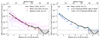 |
Fig. 11. Typical Lyα SB profiles with cosmic dimming corrections scaled to z = 3.65. (a) The violet and blue solid lines show individual SB profiles of LAHs and non-LAHs, respectively. The black solid line and the gray shaded area indicate the mean SB profile of 17 LAHs and the 1σ uncertainty, respectively, while the red dashed line indicates the mean SB profile of 13 isolated LAHs. The black crosses represent the median profile of the 17 LAHs. The black dashed holizontal line shows the typical 1σ SB limit of the mean LAH stack. (b) The blue circles and cyan crosses show the median SB profile of stacked MUSE LAEs at z = 3 − 4 (Wisotzki et al. 2018, W18) and the same data multiplied by 1.85 to compare the profile shapes. |
In an ideal case with higher S/N values, we would be able to estimate the halo size (for instance, 90% luminosity radius) by fitting the SB with two-component Sersic profiles. This would allow us to also probe the halo-size dependence on M1500, which might exist. However, even with the MXDF data set, the S/N is not high enough to constrain the area detected with Lyα in such a sophisticated way. Therefore, following Wisotzki et al. (2018), we calculated the Lyα size corresponding to the typical 1σ SB limit, 5 × 10⁻²¹ erg s−1 cm−2 arcsec−2.
4.2.2. The incidence rate of LAHs
Assuming that LAHs have the same area (ALAH) on average, we calculated the incidence rate of LAHs, dn/dz(LAH), for our sample. We use the UV luminosity function (LF) from Bouwens et al. (2015) at redshift z ≃ 3.8, similar to the midpoint redshift of our sample. This LF has a characteristic magnitude of M⋆ = −20.88 mag, a normalization ϕ* = 1.97 Mpc−3, and a faint-end slope of α = −1.641. A cumulative dn/dz(LAH, M1500 ≤ M1500, 0) for a certain M1500, 0 limit is given as follows:
 (3)
(3)
where n(M1500, 0), VMXDF, AMXDF, and Δz are the number density for M1500 ≤ M1500, 0, the survey volume, the survey area, and the redshift bin width, respectively. We integrated the LF from −23 mag to −18 mag, which is the faintest magnitude in our sample, see Fig. 1c. The obtained dn/dz(LAH, M1500 ≤ −18) is  , whose uncertainty is propagated from the 1σ error of XLAH for all the sources. The lower M1500 limit of −23 mag is brighter than our brightest LAH with M1500 ≃ −20 mag, but the contribution from galaxies with M1500 = −23 to −21 mag to our dn/dz(LAH, M1500 ≤ −18) is small. The high incidence rate of LAHs suggests that about 80% of the sky is covered by the Lyα emission from galaxies with M1500 ≤ −18 mag at z = 3 − 4. The value is similar to that for MUSE LAEs at z = 3 − 4 with their SB limit of ≃1.5 × 10⁻²⁰ erg s−1 cm−2 arcsec−2, 1.0 ± 0.4, but is lower than that for the similar SB limit of ≃5 × 10⁻²¹ erg s−1 cm−2 arcsec−2, 2.3 ± 1.3 (Wisotzki et al. 2018). The difference could be caused by the sample selections as we discussed above for the difference in the SB profiles. We also calculated the dn/dz(LAH, M1500 ≤ M1500, 0) with different M1500, 0, which is shown in Fig. 12 and used in the comparison in Sect. 4.2.3.
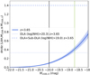 |
Fig. 12. Cumulative incidence rate of LAHs, dn/dz(LAH, M1500 ≤ M1500, 0), as a function of M1500, 0. The blue solid line and shading show the dn/dz(LAH, M1500 ≤ M1500, 0) at z ≃ 3.65 and the uncertainty, respectively. The uncertainty is propagated from the 1σ error of the XLAH for all the sources. The solid black and green lines indicate M1500 of the brightest source in our sample and the upper limit of M1500 for the UV-bright sample, respectively (the M1500 of the faintest source is −18 mag). The blue dashed thin and thick lines represent the dn/dz for DLAs and DLAs+sub-DLAs at z = 3.65 calculated from the best-fit formulae of the z evolution of absorbers in Zafar et al. (2013a). |
4.2.3. The incidence rate of LAHs compared with those of strong Lyα absorbers
We compare the incidence rate of LAHs with those of DLAs and sub-DLAs, dn/dz(DLA) and dn/dz(sub-DLA), at our median redshift (z = 3.65) from Zafar et al. (2013a). They show the best-fit redshift evolution of the observed dn/dz for DLAs and sub-DLAs at z = 0 − 5 by scaling the best-fit relation for LLSs in Songaila & Cowie (2010). As shown in Fig. 12, our  is in between dn/dz(DLA) = 0.33 (blue dashed thick line) and dn/dz(DLA)+dn/dz(sub-DLA) = 1.4 (blue dashed thin line). Our incidence rate for the UV-bright sample, dn/dz(LAH, M1500 ≤ −18.7) (green vertical line), is closer to dn/dz(DLA) but is also located in between them. It suggests that Lyα haloes are counterparts of DLAs and sub-DLAs.
It is interesting to extend the exercise to higher redshifts and fainter M1500 in order to discuss the redshift evolution. We assumed that galaxies have the same ALAH in comoving kpc2 at redshifts of z ≃ 4.9 and z ≃ 5.9 as at z ≃ 3.65 (e.g., Wisotzki et al. 2016; Leclercq et al. 2017). We used UV LFs at z ≃ 4.9 (z ≃ 5.9) from Bouwens et al. (2015), M⋆ = −21.10 mag, ϕ* = 0.79 Mpc−3, and α = −1.76 (M⋆ = −21.10 mag, ϕ* = 0.39 Mpc−3, and α = −1.90). The dn/dz(LAH, M1500 ≤ M1500, 0) were calculated down to M1500, 0 = −14 mag at z ≃ 3.65, z ≃ 4.9 and z ≃ 5.9 in the same manner as in Sect. 4.2.2 (see Fig. 13). The incidence rate of LLSs, dn/dz(LLS), as well as dn/dz(DLA) and dn/dz(sub-DLA), were obtained from the formulae in Songaila & Cowie (2010) and Zafar et al. (2013a), respectively. The results of the abundance matching for DLAs evolve with redshift. At z ≃ 3.7, dn/dz(DLA) can be matched with dn/dz(LAH) with  . Meanwhile, it requires
  and
and  at z ≃ 4.9 and z ≃ 5.9, respectively. The same trends with redshift are found for dn/dz(sub-DLA) and dn/dz(LLS). We need to go to fainter M1500 limits at higher redshifts to provide the same level of dn/dz as that for absorbers.
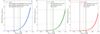 |
Fig. 13. Cumulative incidence rate of LAHs, dn/dz(LAH, M1500 ≤ M1500, 0), as a function of M1500, 0 at different redshifts. The different colors (blue, green, and red) indicate different redshifts (z ≃ 3.65, 4.9, and 5.9 in panels a–c, respectively). The solid black vertical lines show the M1500 of the brightest and faintest sources in our sample. The green vertical line indicates the upper limit of M1500 for the UV-bright sample. (a) At z ≃ 3.65. The blue solid line and shading show the dn/dz(LAH, M1500 ≤ M1500, 0) and the uncertainty, respectively. The blue-dashed thin line, medium-thick line, and thick line represent the dn/dz for DLAs, DLAs+sub-DLAs, and DLAs+sub-DLAs+LLSs at the same redshift, respectively. (b) At z ≃ 4.9. (c) At z ≃ 5.9. |
The z evolution seen in this exercise can be explained by the combination of two redshift evolutions. First, we have the dn/dz evolution of absorbers, which increases with increasing redshifts, implying the presence of denser and more neutral hydrogen gas at higher redshifts. This evolution is expected to be maintained by increasing rates of cold accretion and the higher mean density of the Universe at higher redshifts (Rahmati et al. 2015). Second, the UV LFs evolve. The number density of such relatively bright galaxies decreases with increasing redshifts. Therefore, with the assumption of no dependence of ALAH on z and M1500, fainter M1500 sources are required to be accounted to reproduce dn/dz of absorbers at higher redshifts.
Despite the remarkable progress with the UV-selected, as opposed to Lyα-selected, sample, we caution against overinterpreting the results. The examination here is a very simple abundance matching with assumptions. The dependence of ALAH on z, M1500, or other galaxy’s properties were not considered. Since UV brighter galaxies and lower-z galaxies tend to have a larger UV size than their counterparts (e.g., Shibuya et al. 2015), UV fainter and higher-z galaxies may have a smaller ALAH. Would it be true, dn/dz(LAH, M1500 ≤ M1500, 0) could be overestimated with M1500, 0 ≥ −18 or at z ≃ 5 and ≃6. However, the correlation between M1500 and halo size is under debate (e.g., Steidel et al. 2011; Momose et al. 2016; Xue et al. 2017; Leclercq et al. 2017; Wu et al. 2020; Claeyssens et al. 2022). No clear redshift evolution of the Lyα halo size has been confirmed (e.g., Momose et al. 2014; Leclercq et al. 2017). Last but not least, our modeling is based on a simple abundance matching approach in which one Lyα halo corresponds to one absorber. As shown in Rahmati et al. (2015) and Stern et al. (2021), for example, many absorbers with various N(H I) plausibly make up the CGM of individual high-z galaxies. Simulations of the CGM and absorbers greatly depend on the strength and the implementation of feedback models (Faucher-Giguère et al. 2015; Rahmati et al. 2015; Suresh et al. 2015). Since Lyα emission is the best tracer of the CGM H I gas at high redshifts, which can provide spatial information, our results have great potential to constrain feedback models. It will be challenging as demonstrated in Mitchell et al. (2021), but could also provide information on the mass, extent, dynamics, and physical state of the CGM gas.
4.3. Implications from non-LAHs
It is also interesting that four of our galaxies do not have a significant Lyα halo, though they could be hidden in the noise as discussed in Sect. 3.3.4. Even aside from RID = 22230, which shows potential extended Lyα emission with an anisotropic profile, the remaining three objects may have different reasons for the suppression of extended Lyα emission. RID = 5479 has very bright Lyα emission on the scale of the galaxy’s UV component as shown in Fig. 3, but it does not show extended Lyα. It may imply a small amount of H I gas in the CGM, which allows Lyα photons to escape directly from the galaxy to the IGM. Such a galaxy may differ in halo mass from other galaxies or may be in a different evolutionary phase. A low H I content of the CGM may be due to a phase with weak stellar feedback which does not push the gas out from the ISM to the CGM (see Fig. 11 in Rahmati et al. 2015, and Appendix B in Faucher-Giguère et al. 2015). It could also be caused by a phase with very strong stellar and AGN feedback which either ionizes the gas or significantly disrupts or ejects gas from the CGM (see Sect. 5.2 in Trebitsch et al. 2017). A low fraction of such objects would imply a short duty cycle of the lacking or disrupted phase. RID = 23135 and RID = 54891 have faint Lyα emission inside the galaxy’s UV-component scale, suggesting that Lyα photons produced by the star formation could be killed by the dust in the ISM or the CGM and that the in-situ halo mechanism and satellite scenario do not work for these galaxies. In fact, a wide variety of H I covering fractions are predicted in simulations: around 25%−45% and around 55%−75% as a 15−85 percentile for log(Mh [M⊙]) ≃ 11.1 at z ≃ 3 and z ≃ 4, respectively (Rahmati et al. 2015). It is interesting to explore causes of a poor gas content for rare galaxies in simulations. In particular, galaxies which can allow ionizing photons to escape directly from the ISM to the IGM thanks to the low CGM H I column density would play an important role in cosmic reionization.
5. Conclusions
Thanks to the more than 100-h integration with MUSE AO in the MXDF (Bacon et al. 2021), we were able to examine the existence of Lyα haloes around UV-selected star-forming galaxies at z ≃ 2.9 − 4.4. With the MXDF data, we constructed a sample with a F775W ≤ 27.5 mag cut, with spectroscopic redshift constraints. We confirmed that all of 26 sources with zp ≃ 2.9 − 4.40 have a close spec-z estimation to their photo-z, which implies high completeness values of our spec-z assignments. We used 21 galaxies at zs = 2.9 − 4.4, which include 17 isolated sources in HST images. The M1500 range of our sample is −20 to −18 mag, enabling us to construct a UV-bright sample over the redshift range (11 sources, −20.0 ≤ M1500 ≤ −18.7). Our major results are summarized as follows.
-
Among 21 galaxies, 17 were confirmed to have significant extended Lyα emission. We report the first individual detections of extended Lyα emission around non-LAEs with negative net equivalent widths of Lyα (for instance, RID = 4587 and 4764). We measured the Lyα halo fraction for the sample of all the sources of
 %, for the 17 isolated sources of
  %, and for the 12 −20.0 ≤ M1500 ≤ −18.7 sources of
  %. The XLAH increases to
  %, for nonisolated galaxies, though it is consistent within the 1σ error bars. The high fractions are similar to that for MUSE LAEs, about 80%, in Leclercq et al. (2017), though the methods are different.
 -
The high fractions of Lyα haloes imply that UV-selected galaxies generally have a significant amount of cool/warm gas in the CGM. Our study shows for the first time significant extended Lyα emission around most individual high-z star-forming galaxies in a spec-z complete sample.
-
The mean SB profile for 17 LAHs was derived with cosmic dimming corrections for the midpoint redshift of z ≃ 3.65. The mean Lyα radius above the typical 1σ uncertainty of the SB is 5.4 arcsec (40 kpc).
-
Assuming that extended Lyα emission traces the same cool/warm gas as absorbing systems, we used the abundance matching technique for incidence rates in order to investigate the correspondence between gas detected in absorption and emission. Our dn/dz(LAH) calculated from a UVLF, the typical LAH size, and the measured XLAH is
 for M1500 ≤ −18 mag at z ≃ 3.65. This is in between dn/dz(DLA) and dn/dz(DLA)+dn/dz(sub-DLA) at the same redshift. It suggests that Lyα haloes trace the same gas as DLAs and sub-DLAs.
 -
At higher redshifts, we need to go to a fainter M1500 limit to reach the same dn/dz as that for absorbers (DLA, sub-DLA, and LLSs). At z ≃ 3.7, dn/dz(DLA) can be matched with dn/dz(LAH) with
 , but it requires
  and
and  at z ≃ 4.9 and z ≃ 5.9, respectively. The z evolution is due to the increase of dn/dz for absorbers with z and the decrease of number densities of UV LFs with z.
 -
We found four non-LAHs, though one of them shows potential extended Lyα emission with an anisotropic profile (with M1500 = −18.6). Another one has very bright Lyα emission within the scale of the galaxy’s UV component but does not show extended Lyα (with M1500 = −19.3), implying a small amount of the HI gas in the CGM, which may allow Lyα photons to escape directly from the galaxy to the IGM. The remaining sources have faint Lyα emission inside the galaxy’s UV-component scale (with M1500 = −18.0 and −18.4), suggesting that Lyα photons produced by the star formation could be destroyed by dust in the ISM or the CGM and that the in-situ halo mechanism and satellite scenario are not at play for these galaxies.
We plan to extend this work to photometric-redshift samples in the near future using the MUSE HUDF survey data (9 arcmin2) and upcoming MUSCATEL data (MUSE Cosmic Assembly survey Targetting Extragalactic Legacy fields; in total 36 arcmin2), which will give us a more general view of XLAH. The larger cosmic volume of those surveys compared to that of the MXDF (0.84 arcmin2 in this study) will be useful to extend the dynamic range to brighter galaxies. In order to constrain the physics of Lyα haloes and the trends of galaxies with and without haloes, we will investigate the LAH properties and the properties of the host galaxies with a larger sample. Finally, with MXDF data, our sample will allow spatially resolved spectral analysis of Lyα emission as those in the literature (Claeyssens et al. 2019; Leclercq et al. 2020, see also Patrício et al. 2016; Matthee et al. 2020, as well as Claeyssens et al. 2022 for the Lensed Lyman-Alpha MUSE Arc Sample, LLAMAS).
We note that Bouwens et al. (2015) derive the UVLFs for a longer wavelength (rest-frame 1600 Å) than that used in this study (1500 Å), and we assumed that the wavelength difference can be ignored.
Lyα lines are fit with a skewed Gaussian with an asymmetry parameter γ: ![Mathematical equation: $ F(\lambda) = F_{\mathrm{max}}\left[1 + \mathrm{erf} \left(\gamma\frac{\lambda-\lambda_0}{\sqrt{2}\sigma}\right)\right] \left[\mathrm{exp} \left(-\frac{(\lambda-\lambda_0)^2}{2\sigma^2}\right)\right] $](/articles/aa/full_html/2022/04/aa42302-21/aa42302-21-eq104.gif) , where Fmax, σ, and λ0 represent the amplitude, the width, and the peak wavelength, respectively, and the erf is error function (see Bacon et al. in prep. for more details).
, where Fmax, σ, and λ0 represent the amplitude, the width, and the peak wavelength, respectively, and the erf is error function (see Bacon et al. in prep. for more details).
RID = 7876 and RID = 9944 are treated as a single HST source in the Cosmic Assembly Near-IR Deep Extragalactic Legacy Survey (CANDELS, ID = 110794, Whitaker et al. 2019) and 3D-HST (ID = 28521, Skelton et al. 2014). Following the other MUSE GTO papers, we used the catalog of Rafelski et al. (2015) as a HST prior list (see also Figures C.1 and C.2).
Acknowledgments
We thank the anonymous referee for constructive comments and suggestions. We would like to express our gratitude to Edmund Christian Herenz, Leindert Boogard, Miroslava Dessauges, Moupiya Maji, Valentin Mauerhofer, Charlotte Paola Simmonds Wagemann, Masami Ouchi, Kazuhiro Shimasaku, Akio Inoue, and Rieko Momose for giving insightful comments and suggestions. H.K. is grateful to Liam McCarney for useful suggestions on English writing through the UniGE’s Tandems linguistiques. H.K. acknowledges support from Swiss Government Excellence Scholarships and Japan Society for the Promotion of Science (JSPS) Overseas Research Fellowship. H.K., F.L., and A.V. are supported by the SNF grant PP00P2 176808. A.V. and T.G. are supported by the ERC Starting Grant 757258“TRIPLE”. This work was supported by the Programme National Cosmology et Galaxies (PNCG) of CNRS/INSU with INP and IN2P3, co-funded by CEA and CNES. This work is based on observations taken by VLT, which is operated by European Southern Observatory. This research made use of Astropy, which is a community-developed core Python package for Astronomy (Astropy Collaboration 2013, 2018), and other software and packages: MARZ, MPDAF (Piqueras et al. 2019), PHOTUTILS, Numpy (Harris et al. 2020), Scipy (Virtanen et al. 2020), and matplotlib (Hunter 2007).
References
- Aghanim, N., Akrami, Y., Ashdown, M., et al. 2020, A&A, 641, A6 [NASA ADS] [CrossRef] [EDP Sciences] [Google Scholar]
- Astropy Collaboration (Robitaille, T. P., et al.) 2013, A&A, 558, A33 [NASA ADS] [CrossRef] [EDP Sciences] [Google Scholar]
- Astropy Collaboration (Price-Whelan, A. M., et al.) 2018, AJ, 156, 123 [Google Scholar]
- Bacher, R. 2017, PhD Thesis, University of Michigan [Google Scholar]
- Bacon, R., Accardo, M., Adjali, L., et al. 2010, Proc. SPIE, 7735, 773508 [Google Scholar]
- Bacon, R., Conseil, S., Mary, D., et al. 2017, A&A, 608, A1 [NASA ADS] [CrossRef] [EDP Sciences] [Google Scholar]
- Bacon, R., Mary, D., Garel, T., et al. 2021, A&A, 647, A107 [NASA ADS] [CrossRef] [EDP Sciences] [Google Scholar]
- Baldry, I. K., Alpaslan, M., Bauer, A. E., et al. 2014, MNRAS, 441, 2440 [Google Scholar]
- Barnes, L. A., & Haehnelt, M. G. 2010, MNRAS, 403, 870 [NASA ADS] [CrossRef] [Google Scholar]
- Beckett, A., Morris, S. L., Fumagalli, M., et al. 2021, MNRAS, 26, 1 [Google Scholar]
- Beckwith, S., & Stiavelli, M. 2006, AJ, 132, 1729 [NASA ADS] [CrossRef] [Google Scholar]
- Benitez, N. 2000, ApJ, 536, 571 [CrossRef] [Google Scholar]
- Benitez, N., Ford, H., Bouwens, R., et al. 2004, ApJS, 150, 1 [NASA ADS] [CrossRef] [Google Scholar]
- Bertin, E., & Arnouts, S. 1996, A&A, 117, 393 [Google Scholar]
- Bouwens, R. J., Illingworth, G. D., Oesch, P. A., et al. 2015, ApJ, 803, 1 [NASA ADS] [CrossRef] [Google Scholar]
- Bradley, L., Sipőcz, W. B., Robitaille, T., et al. 2021, https://doi.org/10.5281/zenodo.5796924 [Google Scholar]
- Burchett, J. N., Rubin, K. H. R., Prochaska, J. X., et al. 2021, ApJ, 909, 151 [NASA ADS] [CrossRef] [Google Scholar]
- Byrohl, C., Nelson, D., Behrens, C., et al. 2021, MNRAS, 506, 5129 [NASA ADS] [CrossRef] [Google Scholar]
- Cantalupo, S., Porciani, C., Lilly, S. J., & Miniati, F. 2005, ApJ, 628, 61 [Google Scholar]
- Chen, Y., Steidel, C. C., Erb, D. K., et al. 2021, MNRAS, 508, 19 [NASA ADS] [CrossRef] [Google Scholar]
- Christensen, L., Sánchez, S. F., Jahnke, K., et al. 2004, A&A, 417, 487 [NASA ADS] [CrossRef] [EDP Sciences] [Google Scholar]
- Claeyssens, A., Richard, J., Blaizot, J., et al. 2019, MNRAS, 489, 5022 [Google Scholar]
- Claeyssens, A., Richard, J., Blaizot, J., et al. 2022, A&A, accepted https://doi.org/10.1051/0004-6361/202142320 [Google Scholar]
- Coe, D., Benítez, N., Sánchez, S. F., et al. 2006, AJ, 132, 926 [Google Scholar]
- Davies, J. J., Crain, R. A., Oppenheimer, B. D., & Schaye, J. 2020, MNRAS, 491, 4462 [NASA ADS] [CrossRef] [Google Scholar]
- De Cia, A., Ledoux, C., Petitjean, P., & Savaglio, S. 2018, A&A, 611, A76 [NASA ADS] [CrossRef] [EDP Sciences] [Google Scholar]
- Dessauges-Zavadsky, M., Peroux, C., Kim, T.-S., D’Odorico, S., & McMahon, R. G. 2003, MNRAS, 345, 447 [NASA ADS] [CrossRef] [Google Scholar]
- Dijkstra, M., & Kramer, R. 2012, MNRAS, 424, 1672 [NASA ADS] [CrossRef] [Google Scholar]
- Drake, A. B., Garel, T., Wisotzki, L., et al. 2017, A&A, 608, A6 [NASA ADS] [CrossRef] [EDP Sciences] [Google Scholar]
- Epinat, B., Contini, T., Finley, H., et al. 2018, A&A, 609, A40 [NASA ADS] [CrossRef] [EDP Sciences] [Google Scholar]
- Erb, D. K., Quider, A. M., Henry, A. L., & Martin, C. L. 2012, ApJ, 759, 26 [CrossRef] [Google Scholar]
- Fardal, M. A., Katz, N., Gardner, J. P., et al. 2001, ApJ, 562, 605 [Google Scholar]
- Faucher-Giguère, C.-A., Hopkins, P. F., Kereš, D., et al. 2015, MNRAS, 449, 987 [CrossRef] [Google Scholar]
- Feltre, A., Maseda, M. V., Bacon, R., et al. 2020, A&A, 641, A118 [EDP Sciences] [Google Scholar]
- Finley, H., Bouché, N., Contini, T., et al. 2017, A&A, 605, A118 [NASA ADS] [CrossRef] [EDP Sciences] [Google Scholar]
- Fujimoto, S., Ouchi, M., Ferrara, A., et al. 2019, ApJ, 887, 107 [Google Scholar]
- Fumagalli, M., Prochaska, J. X., Kasen, D., et al. 2011, MNRAS, 418, 1796 [CrossRef] [Google Scholar]
- Fumagalli, M., O’Meara, J. M., Prochaska, J. X., Rafelski, M., & Kanekar, N. 2015, MNRAS, 446, 3178 [NASA ADS] [CrossRef] [Google Scholar]
- Fumagalli, M., Mackenzie, R., Trayford, J., et al. 2017, MNRAS, 471, 3686 [NASA ADS] [CrossRef] [Google Scholar]
- Furlanetto, S. R., Schaye, J., Springel, V., & Hernquist, L. 2005, ApJ, 622, 7 [Google Scholar]
- Garel, T., Blaizot, J., Guiderdoni, B., et al. 2015, MNRAS, 450, 1279 [Google Scholar]
- Garel, T., Blaizot, J., Rosdahl, J., et al. 2021, MNRAS, 504, 1902 [NASA ADS] [CrossRef] [Google Scholar]
- Ginolfi, M., Jones, G. C., Béthermin, M., et al. 2020, A&A, 633, A1 [Google Scholar]
- Haiman, Z., Spaans, M., & Quataert, E. 2000, ApJ, 537, L5 [Google Scholar]
- Harris, C. R., Millman, K. J., van der Walt, S. J., et al. 2020, Nature, 585, 357 [NASA ADS] [CrossRef] [Google Scholar]
- Hashimoto, T., Garel, T., Guiderdoni, B., et al. 2017, A&A, 608, A10 [NASA ADS] [CrossRef] [EDP Sciences] [Google Scholar]
- Hayashino, T., Matsuda, Y., Tamura, H., et al. 2004, AJ, 128, 2073 [Google Scholar]
- Hayes, M., Östlin, G., Schaerer, D., et al. 2013, ApJ, 765, L27 [NASA ADS] [CrossRef] [Google Scholar]
- Herenz, E. C., Urrutia, T., Wisotzki, L., et al. 2017, A&A, 606, A12 [NASA ADS] [CrossRef] [EDP Sciences] [Google Scholar]
- Hilton, M., Conselice, C. J., Roseboom, I. G., et al. 2012, MNRAS, 425, 540 [NASA ADS] [CrossRef] [Google Scholar]
- Hinton, S. R., Davis, T. M., Lidman, C., Glazebrook, K., & Lewis, G. F. 2016, Astron. Comput., 15, 61 [Google Scholar]
- Ho, M.-F., Bird, S., & Garnett, R. 2020, MNRAS, 496, 5436 [NASA ADS] [CrossRef] [Google Scholar]
- Hunter, J. D. 2007, Comput. Sci. Eng., 9, 90 [NASA ADS] [CrossRef] [Google Scholar]
- Illingworth, G. D., Magee, D., Oesch, P. A., et al. 2013, ApJS, 209, 6 [Google Scholar]
- Inami, H., Bacon, R., Brinchmann, J., et al. 2017, A&A, 608, A2 [NASA ADS] [CrossRef] [EDP Sciences] [Google Scholar]
- Jaskot, A. E., Dowd, T., Oey, M. S., Scarlata, C., & McKinney, J. 2019, ApJ, 885, 96 [Google Scholar]
- Johnson, S. D., Chen, H.-W., Mulchaey, J. S., Schaye, J., & Straka, L. A. 2017, ApJ, 850, L10 [NASA ADS] [CrossRef] [Google Scholar]
- Johnson, S. D., Chen, H.-W., Straka, L. A., et al. 2018, ApJ, 869, L1 [Google Scholar]
- Kakiichi, K., & Dijkstra, M. 2018, MNRAS, 5159, 5140 [NASA ADS] [Google Scholar]
- Kakuma, R., Ouchi, M., Harikane, Y., et al. 2021, ApJ, 916, 22 [NASA ADS] [CrossRef] [Google Scholar]
- Kashikawa, N., Misawa, T., Minowa, Y., et al. 2014, ApJ, 780, 116 [Google Scholar]
- Keel, W. C., Cohen, S. H., Windhorst, R. A., & Waddington, I. 1999, AJ, 118, 2547 [NASA ADS] [CrossRef] [Google Scholar]
- Kikuchihara, S., Harikane, Y., Ouchi, M., et al. 2021, ArXiv e-prints [arXiv:2108.09288] [Google Scholar]
- Kollmeier, J. A., Zheng, Z., Davé, R., et al. 2010, ApJ, 708, 1048 [Google Scholar]
- Kornei, K. A., Shapley, A. E., Erb, D. K., et al. 2010, ApJ, 711, 693 [NASA ADS] [CrossRef] [Google Scholar]
- Krogager, J.-K., Møller, P., Fynbo, J. P. U., & Noterdaeme, P. 2017, MNRAS, 469, 2959 [NASA ADS] [CrossRef] [Google Scholar]
- Kunth, D., Leitherer, C., Mas-Hesse, J. M., Östlin, G., & Petrosian, A. 2003, ApJ, 597, 263 [NASA ADS] [CrossRef] [Google Scholar]
- Kusakabe, H., Shimasaku, K., Momose, R., et al. 2019, PASJ, 71, 1 [NASA ADS] [CrossRef] [Google Scholar]
- Kusakabe, H., Blaizot, J., Garel, T., et al. 2020, A&A, 638, A12 [NASA ADS] [CrossRef] [EDP Sciences] [Google Scholar]
- Lake, E., Zheng, Z., Cen, R., et al. 2015, ApJ, 806, 46 [NASA ADS] [CrossRef] [Google Scholar]
- Lanzetta, K. M., Bowen, D. B., Tytler, D., & Webb, J. K. 1995, ApJ, 442, 538 [NASA ADS] [CrossRef] [Google Scholar]
- Laursen, P., & Sommer-Larsen, J. 2007, ApJ, 657, L69 [NASA ADS] [CrossRef] [Google Scholar]
- Leclercq, F., Bacon, R., Wisotzki, L., et al. 2017, A&A, 608, A8 [NASA ADS] [CrossRef] [EDP Sciences] [Google Scholar]
- Leclercq, F., Bacon, R., Verhamme, A., et al. 2020, A&A, 635, A82 [NASA ADS] [CrossRef] [EDP Sciences] [Google Scholar]
- Leclercq, F., Verhamme, A., Epinat, B., et al. 2022, ArXiv e-prints [arXiv:2203.05614] [Google Scholar]
- Li, J.-T., & Wang, Q. D. 2013, MNRAS, 435, 3071 [NASA ADS] [CrossRef] [Google Scholar]
- Mackenzie, R., Fumagalli, M., Theuns, T., et al. 2019, MNRAS, 487, 5070 [NASA ADS] [CrossRef] [Google Scholar]
- Martin, C. L., Shapley, A. E., Coil, A. L., et al. 2013, ApJ, 770, 41 [NASA ADS] [CrossRef] [Google Scholar]
- Mary, D., Bacon, R., Conseil, S., Piqueras, L., & Schutz, A. 2020, A&A, 635, A194 [EDP Sciences] [Google Scholar]
- Mas-Ribas, L., & Dijkstra, M. 2016, ApJ, 822, 84 [Google Scholar]
- Mas-Ribas, L., Dijkstra, M., Hennawi, J. F., et al. 2017a, ApJ, 841, 19 [Google Scholar]
- Mas-Ribas, L., Hennawi, J. F., Dijkstra, M., et al. 2017b, ApJ, 846, 11 [NASA ADS] [CrossRef] [Google Scholar]
- Matsuda, Y., Yamada, T., Hayashino, T., et al. 2011, MNRAS, 410, 13 [Google Scholar]
- Matsuda, Y., Yamada, T., Hayashino, T., et al. 2012, MNRAS, 425, 878 [NASA ADS] [CrossRef] [Google Scholar]
- Matthee, J., Sobral, D., Oteo, I., et al. 2016, MNRAS, 458, 449 [Google Scholar]
- Matthee, J., Pezzulli, G., Mackenzie, R., et al. 2020, MNRAS, 498, 3043 [Google Scholar]
- Matthee, J., Sobral, D., Hayes, M., et al. 2021, MNRAS, 505, 1382 [NASA ADS] [CrossRef] [Google Scholar]
- McKinney, J. H., Jaskot, A. E., Oey, M. S., et al. 2019, ApJ, 874, 52 [NASA ADS] [CrossRef] [Google Scholar]
- Mitchell, P. D., Blaizot, J., Cadiou, C., et al. 2021, MNRAS, 5775, 5757 [Google Scholar]
- Moffat, A. F. J. 1969, A&A, 3, 455 [NASA ADS] [Google Scholar]
- Momose, R., Ouchi, M., Nakajima, K., et al. 2014, MNRAS, 442, 110 [NASA ADS] [CrossRef] [Google Scholar]
- Momose, R., Ouchi, M., Nakajima, K., et al. 2016, MNRAS, 457, 2318 [NASA ADS] [CrossRef] [Google Scholar]
- Morrissey, P., Matuszewski, M., Martin, D. C., et al. 2018, ApJ, 864, 93 [Google Scholar]
- Muzahid, S., Schaye, J., Cantalupo, S., et al. 2021, MNRAS, 508, 5612 [NASA ADS] [CrossRef] [Google Scholar]
- Nelson, D., Pillepich, A., Springel, V., et al. 2019, MNRAS, 490, 3234 [Google Scholar]
- Nelson, D., Byrohl, C., Peroux, C., Rubin, K. H. R., & Burchett, J. N. 2021, MNRAS, 507, 4445 [NASA ADS] [CrossRef] [Google Scholar]
- Noterdaeme, P., Petitjean, P., Carithers, W. C., et al. 2012, A&A, 547, A1 [NASA ADS] [CrossRef] [EDP Sciences] [Google Scholar]
- Oke, J. B., & Gunn, J. E. 1983, ApJ, 266, 713 [NASA ADS] [CrossRef] [Google Scholar]
- Oppenheimer, B. D., & Davé, R. 2008, MNRAS, 387, 577 [NASA ADS] [CrossRef] [Google Scholar]
- Oppenheimer, B. D., Crain, R. A., Schaye, J., et al. 2016, MNRAS, 460, 2157 [NASA ADS] [CrossRef] [Google Scholar]
- Östlin, G., Hayes, M., Kunth, D., et al. 2009, AJ, 138, 923 [NASA ADS] [CrossRef] [Google Scholar]
- Ouchi, M., Ono, Y., & Shibuya, T. 2020, ARA&A, 58, 617 [Google Scholar]
- Patrício, V., Richard, J., Verhamme, A., et al. 2016, MNRAS, 456, 4191 [Google Scholar]
- Peeples, M. S., Corlies, L., Tumlinson, J., et al. 2019, ApJ, 873, 129 [Google Scholar]
- Peroux, C., Dessauges-Zavadsky, M., D’Odorico, S., Kim, T.-S., & McMahon, R. G. 2003, MNRAS, 345, 480 [NASA ADS] [CrossRef] [Google Scholar]
- Péroux, C., & Howk, J. C. 2020, ARA&A, 58, 363 [CrossRef] [Google Scholar]
- Pillepich, A., Nelson, D., Springel, V., et al. 2019, MNRAS, 490, 3196 [Google Scholar]
- Piqueras, L., Conseil, S., Shepherd, M., et al. 2019, ASP Conf. Ser., 521, 545 [Google Scholar]
- Prochaska, J. X., Herbert-Fort, S., & Wolfe, A. M. 2005, ApJ, 635, 123 [NASA ADS] [CrossRef] [Google Scholar]
- Prochaska, J. X., Hennawi, J. F., Lee, K.-G., et al. 2013, ApJ, 776, 136 [NASA ADS] [CrossRef] [Google Scholar]
- Rafelski, M., Teplitz, H. I., Gardner, J. P., et al. 2015, AJ, 150, 31 [Google Scholar]
- Rahmati, A., Schaye, J., Bower, R. G., et al. 2015, MNRAS, 452, 2034 [CrossRef] [Google Scholar]
- Rauch, M., Haehnelt, M., Bunker, A., et al. 2008, ApJ, 681, 856 [NASA ADS] [CrossRef] [Google Scholar]
- Rosdahl, J., & Blaizot, J. 2012, MNRAS, 423, 344 [Google Scholar]
- Rubin, K. H., Prochaska, J. X., Ménard, B., et al. 2011, ApJ, 728, 6 [NASA ADS] [CrossRef] [Google Scholar]
- Rubin, K. H., Hennawi, J. F., Prochaska, J. X., et al. 2015, ApJ, 808, 38 [NASA ADS] [CrossRef] [Google Scholar]
- Rudie, G. C., Steidel, C. C., Trainor, R. F., et al. 2012, ApJ, 750, 67 [NASA ADS] [CrossRef] [Google Scholar]
- Schaye, J., Crain, R. A., Bower, R. G., et al. 2015, MNRAS, 446, 521 [Google Scholar]
- Schroetter, I., Bouché, N., Wendt, M., et al. 2016, ApJ, 833, 39 [NASA ADS] [CrossRef] [Google Scholar]
- Schroetter, I., Bouché, N. F., Zabl, J., et al. 2021, MNRAS, 501, 1900 [NASA ADS] [Google Scholar]
- Shibuya, T., Ouchi, M., & Harikane, Y. 2015, ApJS, 219, 15 [Google Scholar]
- Skelton, R. E., Whitaker, K. E., Momcheva, I. G., et al. 2014, ApJS, 214, 24 [Google Scholar]
- Smith, A., Ma, X., Bromm, V., et al. 2019, MNRAS, 484, 39 [NASA ADS] [CrossRef] [Google Scholar]
- Songaila, A., & Cowie, L. L. 2010, ApJ, 721, 1448 [NASA ADS] [CrossRef] [Google Scholar]
- Spitzer, L., Jr. 1956, ApJ, 124, 20 [NASA ADS] [CrossRef] [Google Scholar]
- Steidel, C. C., Kollmeier, J. A., Shapley, A. E., et al. 2002, ApJ, 570, 526 [NASA ADS] [CrossRef] [Google Scholar]
- Steidel, C. C., Bogosavljević, M., Shapley, A. E., et al. 2011, ApJ, 736, 160 [NASA ADS] [CrossRef] [Google Scholar]
- Stern, J., Sternberg, A., Faucher-Giguère, C.-A., et al. 2021, MNRAS, 507, 2869 [NASA ADS] [CrossRef] [Google Scholar]
- Suresh, J., Bird, S., Vogelsberger, M., et al. 2015, MNRAS, 448, 895 [NASA ADS] [CrossRef] [Google Scholar]
- Swinbank, A. M., Bower, R. G., Smith, G. P., et al. 2007, MNRAS, 376, 479 [NASA ADS] [CrossRef] [Google Scholar]
- Taniguchi, Y., & Shioya, Y. 2000, ApJ, 532, L13 [NASA ADS] [CrossRef] [Google Scholar]
- Trebitsch, M., Blaizot, J., Rosdahl, J., Devriendt, J., & Slyz, A. 2017, MNRAS, 470, 224 [Google Scholar]
- Tumlinson, J., Peeples, M. S., & Werk, J. K. 2017, ARA&A, 55, 389 [Google Scholar]
- Turner, M. L., Schaye, J., Steidel, C. C., Rudie, G. C., & Strom, A. L. 2014, MNRAS, 445, 794 [NASA ADS] [CrossRef] [Google Scholar]
- Turner, M. L., Schaye, J., Crain, R. A., et al. 2017, MNRAS, 471, 690 [NASA ADS] [CrossRef] [Google Scholar]
- Tytler, D. 1982, Nature, 298, 427 [NASA ADS] [CrossRef] [Google Scholar]
- Urrutia, T., Wisotzki, L., Kerutt, J., et al. 2019, A&A, 624, A1 [Google Scholar]
- Van de Voort, F., Schaye, J., Altay, G., & Theuns, T. 2012, MNRAS, 421, 2809 [NASA ADS] [CrossRef] [Google Scholar]
- Verhamme, A., Schaerer, D., & Maselli, A. 2006, A&A, 460, 397 [NASA ADS] [CrossRef] [EDP Sciences] [Google Scholar]
- Verhamme, A., Dubois, Y., Blaizot, J., et al. 2012, A&A, 546, A111 [NASA ADS] [CrossRef] [EDP Sciences] [Google Scholar]
- Verhamme, A., Garel, T., Ventou, E., et al. 2018, MNRAS, 478, L60 [Google Scholar]
- Virtanen, P., Gommers, R., Oliphant, T. E., et al. 2020, Nat. Meth., 17, 261 [Google Scholar]
- Weilbacher, P. M., Palsa, R., Streicher, O., et al. 2020, A&A, 641, A28 [NASA ADS] [CrossRef] [EDP Sciences] [Google Scholar]
- Werk, J. K., Prochaska, J. X., Tumlinson, J., et al. 2014, ApJ, 792, 8 [NASA ADS] [CrossRef] [Google Scholar]
- Werk, J. K., Prochaska, J. X., Cantalupo, S., et al. 2016, ApJ, 833, 54 [NASA ADS] [CrossRef] [Google Scholar]
- Whitaker, K. E., Ashas, M., Illingworth, G., et al. 2019, ApJS, 244, 16 [CrossRef] [Google Scholar]
- Wilson, E. B. 1927, J. Am. Stat. Assoc., 22, 209 [CrossRef] [Google Scholar]
- Wisotzki, L., Bacon, R., Blaizot, J., et al. 2016, A&A, 587, A98 [NASA ADS] [CrossRef] [EDP Sciences] [Google Scholar]
- Wisotzki, L., Bacon, R., Brinchmann, J., et al. 2018, Nature, 562, 229 [Google Scholar]
- Wolfe, A. M., Turnshek, D. A., Smith, H. E., & Cohen, R. D. 1986, ApJS, 61, 249 [NASA ADS] [CrossRef] [Google Scholar]
- Wolfe, A. M., Gawiser, E., & Prochaska, J. X. 2005, ARA&A, 43, 861 [NASA ADS] [CrossRef] [Google Scholar]
- Wu, J., Jiang, L., & Ning, Y. 2020, ApJ, 891, 105 [NASA ADS] [CrossRef] [Google Scholar]
- Xue, R., Lee, K.-S., Dey, A., et al. 2017, ApJ, 837, 172 [NASA ADS] [CrossRef] [Google Scholar]
- Yajima, H., Li, Y., & Zhu, Q. 2013, ApJ, 773, 151 [NASA ADS] [CrossRef] [Google Scholar]
- Yuma, S., Ouchi, M., Drake, A. B., et al. 2013, ApJ, 779, 53 [NASA ADS] [CrossRef] [Google Scholar]
- Yuma, S., Ouchi, M., Drake, A. B., et al. 2017, ApJ, 841, 93 [NASA ADS] [CrossRef] [Google Scholar]
- Zabl, J., Bouché, N. F., Schroetter, I., et al. 2019, MNRAS, 485, 1961 [NASA ADS] [CrossRef] [Google Scholar]
- Zabl, J., Bouché, N. F., Wisotzki, L., et al. 2021, MNRAS, 507, 4294 [NASA ADS] [CrossRef] [Google Scholar]
- Zafar, T., Popping, A., & Péroux, C. 2013a, A&A, 556, A140 [NASA ADS] [CrossRef] [EDP Sciences] [Google Scholar]
- Zafar, T., Péroux, C., Popping, A., et al. 2013b, A&A, 556, A141 [NASA ADS] [CrossRef] [EDP Sciences] [Google Scholar]
- Zhang, H., Zaritsky, D., Zhu, G., Ménard, B., & Hogg, D. W. 2016, ApJ, 833, 276 [NASA ADS] [CrossRef] [Google Scholar]
- Zhang, H., Ouchi, M., Itoh, R., et al. 2020, ApJ, 891, 177 [NASA ADS] [CrossRef] [Google Scholar]
- Zheng, Z., Cen, R., Weinberg, D., Trac, H., & Miralda-Escudé, J. 2011, ApJ, 739, 62 [NASA ADS] [CrossRef] [Google Scholar]
Appendix A: Details of the sample
A.1. MXDF catalog construction
Here we give a short summary of the MXDF catalog construction and the full explanation is given in Bacon et al. (in prep.). The MUSE MXDF catalog was constructed in two ways and was merged into one catalog: a blind source detection with the 3D matched filtering software, ORIGIN (Mary et al. 2020), and source extraction and deblending based on HST prior information with the ODHIN software (Bacher 2017), in a similar manner to those used in the MUSE-HUDF catalog (Inami et al. 2017; Bacon et al. in prep.). ORIGIN is optimized for the detection of compact sources with faint spatial-spectral emission signatures in MUSE datacubes. It subtracts the continuum from the MUSE cube first, and the detection is based on the local maxima of generalized likelihood ratio test statistics obtained for a set of spatial-spectral profiles of emission line emitters. It provides an estimation of the purity. The threshold value of the purity in the MXDF catalog is 0.8 (i.e., a false detection rate of 0.2). The ODHIN software performs deblending of sources in MUSE datacubes, based on the prior information from HST images with a higher spatial resolution (Rafelski et al. 2015). The selection cut for the prior sources is a S/N of 0.8 per spectral pixel. We extracted 1D spectra at the position of the ORIGIN-detected sources and that of the ODHIN HST-prior sources from the 3D data cube for the redshift determination and visual inspection. To assign redshifts, we used an updated version of the redshift fitting software, MARZ, which is based on a cross-correlation algorithm (e.g., Hilton et al. 2012; Baldry et al. 2014, see also Inami et al. 2017) for both ORIGIN and ODHIN sources. The redshift solutions provided by MARZ were visually inspected by the MUSE team members independently with the source inspector software (Bacon et al. in prep.). We assigned HST counterparts from the Rafelski et al. (2015) catalog when available, and merged an ORIGIN and an ODHIN source into one when they overlapped by choosing the detection method. After reconciliating conclusions between the different inspectors, we summarized sources into the final catalog.
Following Inami et al. (2017) with some improvements, we have three levels of confidence for spec-z (ZCONF). ZCONF = 1 is for a possible redshift with low confidence. It can be assigned due to low S/N values of lines (e.g., S/N ≲ 3), poor line fittings, existence of valid alternative redshift solutions, noisy narrow bands, or additional lines which present in the spectrum with reasonable S/Ns but can not be explained by the proposed redshift solutions. ZCONF = 2 is for a good redshift. Regarding non-Lyα emitters (e.g., z ≲ 2.9), it is assigned for sources with multiple lines detected with good S/N values of S/N ≳ 5. For instance, a resolved [O II]λλ3726,3729 doublet with a clear narrow band would be sufficient for ZCONF = 2. Regarding Lyα emitters, it is required to have a Lyα line with a good S/N of S/N ≳ 5 and a width and an asymmetry compatible with Lyα line shapes. The highest level, ZCONF = 3, indicates a secure redshift. For non-Lyα emitters, the criteria are similar to those of ZCONF = 2, but it is required to have more lines and higher S/N, together with high S/N narrow band images. For Lyα emitters, if there is no additional line except for Lyα, it is required to have a Lyα line with a high S/N value of S/N ≳ 7 and a Lyα-like line profile: a pronounced red asymmetrical line profile2 (highly asymmetric of γ > 2) and/or a blue bump, or a double peaked line profile. The S/N thresholds are not strictly defined because other information was taken into account. In the case of an ORIGIN detection, and if the source can be matched to an HST counterpart, it adds confidence to the detection. In addition, if a photo-z is reliable and a good match to the MUSE spec-z, it adds confidence to the redshift assignment. This could lead to a higher ZCONF than in the case of an ORIGIN source without HST counterpart. Meanwhile, faint HST sources often do not have a reliable photo-z, which can be in disagreement with a MUSE spec-z. It is not taken as a strong negative constraint (see Bacon et al. in prep.). In addition to the three ZCONF levels, ZCONF = 0 is defined in the MXDF catalog (DR2 v0.8) for a source with an ORIGIN detection for which no spectroscopic redshift could be identified. However, in this paper, we independently defined ZCONF = 0 as no spec-z in the MXDF catalog with a tentative (best-estimate) assignment of a redshift or a constraint of a redshift.
A.2. Spec-z and photo-z distribution
In order to check a potential bias in our sample selection, we plotted the distribution of photo-z and spec-z for 142 F775W < 27.5 mag sources from Rafelski et al. (2015) in the MXDF with more than 100-hour integration (see Figure A.1). As described in Section 2.2, 123 sources have ZCONF = 2 or 3, 10 sources have ZCONF = 1, and 9 sources are not included in the MXDF catalog (ZCONF = 0). Most of the ZCONF = 1 to 3 sources have a spec-z, which is consistent with their photo-z (blue and red stars). RID = 23135 is the single ZCONF = 1 source in our sample (red star with zs = 3.94 and  ). Although the photo-z and the spec-z do not match, the source has a strong ORIGIN-detected Lyα emission with S/N = 6.4. Regarding ZCONF = 0 sources (magenta circles), 7 sources were suggested to be at z < 2.86 from clear continua at the blue edge of the MUSE spectra, which are consistent with their photo-z. The remaining two sources, RID = 54891 and 6693, were included in our sample to minimize a selection bias despite ZCONF = 0. The tentative spec-z for RID = 54891 was determined from a low-S/N Lyα line at zs = 2.94, while it was based on a Lyα break and stacks of low-S/N UV absorption lines for RID = 6693 (see Sect. 2.2 for the process of spec-z assignment). Although not all the sources have a secure or reliable spec-z, our spec-z estimations are almost complete with F775W < 27.5 mag.
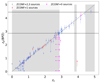 |
Fig. A.1. Photo-z vs. spec-z for 142 F775W < 27.5 mag sources. The blue stars, the red stars, and the magenta dots represent galaxies with ZCONF = 2 or 3, 1, and 0, respectively. The gray shaded areas indicate the spec-z outside the targeted redshift (z = 2.86 − 4.44) and the AO gap. The gray diagonal line and the black lines show the zp = zs relation, and zp = 2.86 and 4.44 lines, respectively. The photometric redshifts were estimated in Rafelski et al. (2015) with the Bayesian Photometric Redshift (BPZ) algorithm (Benitez 2000; Benitez et al. 2004; Coe et al. 2006). The error bars of zp show 95% upper and lower limits. |
Generally, at z ≃ 3 − 6, the Lyα line is the most common zs indicator in follow-up observations, which could introduce a certain sample bias in favor of Lyα emission. We also checked spec-z estimates for zp ≳ 3 sources with F775W < 27.5 mag. Among 142 sources, 26 sources have a best-fit photo-z in 2.86 ≤ zp ≤ 4.44 (between the black lines). All of them except for RID = 6693 have a spec-z with ZCONF = 2 or 3, most of which are consistent with their photo-z. As LAE fractions are not high (e.g., Kusakabe et al. 2020), it means that our sample construction is not significantly biased a Lyα selection despite the redshift range. This result reinforces the high spec-z completeness in our sample construction.
A.3. Lyα equivalent width and LAE fraction
We used rest-frame EW(Lyα) measurements to confirm the presence of LAHs around non-LAEs in Section 3.3.3 and to compare the XLAE with a given EW(Lyα) cut for that in Kusakabe et al. (2020) in Section 2.2 in order to validate that our sample is not biased s the LAE selection. Therefore, the EW(Lyα) values in this paper were measured in the galaxy’s stellar-component scale following Kusakabe et al. (2020). Here we give a brief summary of the methods for the EW(Lyα) measurements and the XLAE calculations. We note that investigating Lyα line properties including EW(Lyα) for our individual sources is beyond the scope of this paper. We plan to improve the method for measuring EW(Lyα) in the MUSE 3D cube and discuss them in a future project.
We extracted the 1D spectra inside the target’s continuum-component mask (hereafter, inside spectra). Some fraction of our sources shows a wide Lyα absorption feature that could extend up to λ ≃ 1 260 Å or even longer. Indeed, Lyα absorption troughs have already been identified for individual LBGs at z ≃ 3 (Kornei et al. 2010, see also Chen et al. 2021), though the feature has not frequently been found for spectra of individual high-z galaxies perhaps because of limited S/N values. Some of our sources also show a Lyα emission line on top of the wide absorption feature (c.f., about 10% of the sample in Kornei et al. 2010), which are similar to local Green Pea galaxies (e.g., McKinney et al. 2019; Jaskot et al. 2019) as well as stacked MUSE LAEs at z ∼ 2.9 − 4.6 (e.g., Feltre et al. 2020). Thanks to the very deep MUSE data, we need to go beyond the standard method for EW(Lyα) measurements for high-z galaxies. We measured the EW(Lyα) for Lyα emission and Lyα absorption (EW(Lyα)emi. and EW(Lyα)abs., respectively) on the inside spectra with a method based on a similar idea in, for instance, Kornei et al. (2010) and calculated the net EW(Lyα), EW(Lyα)net., by summing EW(Lyα)emi. and EW(Lyα)abs. (similar idea to that in McKinney et al. 2019; Jaskot et al. 2019). Figure A.2 shows the 1D spectra of the two non-LAEs with LAHs discussed in Section 3.3.3 as examples of our inside spectra. First of all, we estimated the continuum spectrum around Lyα by fitting the inside spectrum at rest-frame λ ≥ 1270 Å with power-law models (see Sect. 4.3 in Matthee et al. 2021, for the choice of the wavelength limit). To obtain a Lyα emission flux, we integrated Lyα fluxes above the best-fit power-law continuum within a spectral window, whose fluxes are consecutively above the best-fit power-law around the Lyα peak (the blue shaded area). The EW(Lyα)emi. was calculated by dividing the emission flux with the continuum at the Lyα wavelength estimated from the power-law model and converted to that in the rest frame. Regarding the Lyα absorption, we estimated the absorption flux only from redder wavelengths than the Lyα wavelength, as the bluer wavelengths are generally affected by the IGM absorption. We defined the spectral window to measure the absorption fluxes (the orange shaded area). The blue edge of the absorption window is the next wavelength slice of the red edge of the emission window. The red edge of the absorption window was defined with the spectrum extracted in the same target’s continuum-component mask from the continuum minicube (hereafter inside continuum spectrum; Section 2.3). The red edge corresponds to the longest wavelength pixel among the consecutive increasing pixels at the redder side of the blue edge, where the flux on the inside continuum spectrum (the black line) is fainter than that of the best-fit continuum (the magenta line). Considering the possible contamination of N Vλ1243 P-Cygni profile and the limited S/N of the inside spectra for all the sources, we gave a conservative upper limit of the red edge as 1230 Å. We integrated relative fluxes to the power-law continuum within the spectral window. Then, we obtained the Lyα absorption flux by multiplying two to the integrated flux. We calculated EW(Lyα)abs. by dividing the negative absorption flux with the continuum at the Lyα wavelength and converted it to that in the rest-frame. These EW(Lyα)abs. values would be actually the upper limits of the true EW(Lyα) for absorption because of the limited spectral windows (the orange shades). In this work, non-LAEs were defined with EW(Lyα)net. = EW(Lyα)emi. + EW(Lyα)abs. ≤ 0 Å. The two non-LAEs with LAHs introduced in Section 3.3.3, RID = 4587 and 4764, have EW(Lyα)net. ≤ −10.0 ± 2.9 Å and −14.2 ± 1.0 Å, respectively. Moreover, their EW(Lyα)emi. are as small as 2.8 ± 0.6 Å and 0.7 ± 0.3 Å, respectively. Even when we ignore the Lyα absorption (EW(Lyα)abs. ≤ −12.7 ± 2.8 Å and −14.9 ± 1.0 Å, respectively), their EW(Lyα)emi. values are too low to be categorized as LAEs with the typical 20 Å selection criteria. Their EW(Lyα)emi. are also significantly smaller than the minimum EW(Lyα) of the MUSE LAEs with LAHs in Leclercq et al. (2017), ∼20 Å though Lyα halo fluxes are included in their EW(Lyα). These results validate our first individual detections of LAHs around high-z non-LAEs.
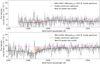 |
Fig. A.2. 1D spectra of the two non-LAEs with LAHs, RID = 4587 and 4764 discussed in Section 3.3.3, as examples of our inside spectra. The dark gray lines, the faint gray shaded areas, the black lines, and the magenta lines show the inner spectra, its 1σ uncertainties, the inner continuum spectra, and the best-fit power-law models for the continua, respectively. The blue and orange shaded areas indicate fluxes integrated for the Lyα emission and Lyα absorption measurements (the spectral windows, see Appendix A.3 for more details), respectively. We note that the Lyα absorption flux (more precisely, the upper limit of the absorption flux) was obtained by multiplying two to the integrated flux in the orange shaded spectral window. |
The LAE fractions for our sample were calculated with EW(Lyα)emi. in a similar method in that of Kusakabe et al. (2020) using the MUSE-HUDF data, which cannot take Lyα absorption into account as their continua are not detected in the MUSE spectra (i.e., nondetection of absorption) for most of the sources. Lyα fluxes from extended emission were not included in the EW(Lyα) for both samples. We did not correct the incompleteness of the detection of Lyα emission for our sample as the completeness is expected to be high, and we estimated the uncertainties on the XLAE from the binomial proportion confidence interval. The XLAE with the typical threshold for LAE selections, EW(Lyα)≥20 Å, for out entire sample with −20 ≤ M1500 ≤ −18.0 at z = 2.9 − 4.4 is  . For a fair comparison, we also calculated the XLAE with EW(Lyα)≥65 Å for our entire sample as
  . As discussed in Section 2.2, this value is similar to those in Kusakabe et al. (2020), suggesting that our sample is not biased.
A.4. nonisolated sources
As described in Section 2.2, our sample includes four nonisolated galaxies, which have a neighboring galaxy with an HST detection within  (Inami et al. 2017) with close spec-z (|ΔV|≲500 km s−1). Figure A.3 shows a NB image of a nonisolated galaxy. RID = 4838 at zs = 3.06 (F775W = 26.70, ZCONF = 2) has a UV-faint neighbor RID = 6666 at zs = 3.06 (F775W = 29.72, ZCONF = 2) with ORIGIN-detected Lyα emission, which is not included in our sample. Interestingly, these sources are a part of a cosmic web filament found with MUSE in Bacon et al. (2021), called “G02”, whose structure extends to a total length of 1.1 pMpc with a width of 47 kpc (see their Fig. 12). Therefore, RID = 4838 was categorized as a nonisolated galaxy.
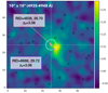 |
Fig. A.3. Lyα NB centered at RID = 4838. The Lyα NB was extracted from the MXDF data cube with a wavelength range of 4935−4948 Å and a size of 10″ × 10″ by source inspector, which was used to visually inspect the MXDF sources. The color bar shows the flux with an arbitrary normalization. The filled pink and filled purple circles indicate a nonisolated galaxy in our sample and its neighbor, which is not included in our sample with a spec-z measurement, respectively. The black open circles show sources in the catalog of Rafelski et al. (2015). The cyan circle indicates a |

As shown in Figure A.4, RID = 7876 (F775W = 26.85) and RID = 9944 (F775W = 26.49) are located within  each other. Because of the limited spatial resolution of MUSE, a MUSE source (MID = 103, zs = 2.99, ZCONF = 3), which shows Lyα emission and absorption depending on wavelength and position, conservatively has two HST counterparts of RID = 7876 and RID = 9944. The Lyα absorption feature gets stronger at the position of RID = 9944 than that of RID = 78763. Moreover, MID = 103 is also within
  from RID = 7847 at zs = 3.00 (F775W = 26.84, ZCONF = 3). Near them, we can see an HST non-detected source at zs = 3.00 (ZCONF = 2, MID = 8246) and a potential neighbor of RID = 7758 at zp = 2.89 (F775W = 28.20). These sources are also included in an overdensity of MUSE-detected LAEs, “G01” (Bacon et al. 2021). As a conservative choice, we categorized RID = 7847 as a nonisolated galaxy, in addition to RID = 7876 and 9944.
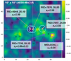 |
Fig. A.4. Same as Figure A.3, but for RIDs = 7847, 7876, and 9944. The Lyα NB is centered at RID = 7876 with a wavelength range of 4838−4863 Å and a size of 10″ × 10″. The filled pink circles indicate three nonisolated galaxies in our sample. The purple open square shows a close MUSE-detected Lyα emitter without an HST counterpart. The purple open circle presents a potential neighbor, which does not have a spec-z but has a close photo-z. The black open circles show sources in the catalog of Rafelski et al. (2015). The cyan circles indicate |

In summary, we conclude that the environments around four nonisolated galaxies in our sample would be different from those of the rest of the galaxies in our sample, which may affect halo properties. We calculated Lyα halo fractions separately for the isolated sources and the nonisolated sources in Section 3.4 for a conservative discussion.
Appendix B: Continuum subtraction
Figure B.1 shows two examples of the difference in the radial SB profiles for the four different settings of the continuum subtractions. One of the objects, which has an artificial absorption trough on the SB profile with the general setting of a 200-pix (±100-pix) window, is RID = 4764. The artificial absorption becomes less significant with the smaller spectral windows. Although the profile inside the target’s continuum-component mask changes depending on the settings of the continuum subtraction, the profiles at r = rin − rCoG are independent of the settings. Another example is RID = 9863, which has a neighbor that cannot be eliminated only by the neighboring object mask. The right panels emphasize the fact that the continuum subtraction is essential to remove neighboring continuum-detected objects from the minicube. The neighboring object masks can only cover continuum-bright objects and prevent uncertainties due to continuum subtractions. Therefore, we needed both of the continuum subtractions and the neighboring object masks. The second example also shows that the SB profiles at r = rin − rCoG are independent of the settings except around neighbors, implying that our tests for the existence of a Lyα halo at r = rin − rCoG are robust and stable.
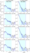 |
Fig. B.1. Examples of the difference in the radial SB profiles for four different settings of the continuum subtractions. The black and blue lines indicate the SB profiles for the original minicubes and the continuum-subtracted minicubes, respectively. The neighboring masks were applied for both. The cyan shaded areas indicate the radii outside the target’s continuum-component masks and inside the rCoG. Left column: RID = 4764, which has an artificial absorption trough with the general setting of a 200-pix (±100-pix) window. Right column: RID = 9863, which has a neighbor (at the radius shown by the magenta solid line) that cannot be eliminated only by the neighboring object mask. From top to bottom, each panel represents the settings: 1) 200-pix (±100-pix) window, 2) 200-pix (±100-pix) window + Lyα mask (±400 km s−1 around Lyα), 3) 100-pix (±50-pix) window + Lyα mask, and 4) 60-pix (±30-pix) window + Lyα mask, respectively. |
Appendix C: Masks
Figures C.1 and C.2 show 4″ × 4″ HST F775W cutout images, 4″ × 4″ cutouts of the HST segmentation map, the target’s continuum-component masks (in the spatial resolution of MUSE, 15″ × 15″), and the neighboring object masks (in the spatial resolution of MUSE, 15″ × 15″), respectively. We used the HST segmentation map in Rafelski et al. (2015) following Inami et al. (2017), which indicates areas in which galaxies are detected and defines the boundaries of the objects. The segmentation map was created with Source Extractor (Bertin & Arnouts 1996) with multiple thresholds for detection and deblending, in order to deblend sources and optimize detections and photometries, as no single set of such thresholds perfectly detects bright, faint, large, and small sources simultaneously (see Sect. 3.5 and Table 2 in Rafelski et al. 2015). They had four iterations. The parameter set for the first iteration is called “Deep” with detect_thresh = 1.1σ and detect_minarea = 9, with which source definitions near bright targets were poorly defined. The second “Shallow” run has detect_thresh = 3.5σ and gave better detections for bright sources. They merged the two catalogs into one, but both runs have difficulty in deblending sources. Then, they had two more iterations called “Deep Deblend” and “Shallow Deblend”, which are with normal deblending parameters and lower deblending thresholds (see their Table 2). The resulting catalogs are merged into a single catalog with a single segmentation map (Rafelski et al. 2015).
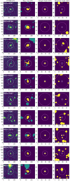 |
Fig. C.1. HST cutouts, segmentation maps, and masks for the first 10 sources in order of RID. First column: 4″ × 4″ HST F775W cutout images. The purple dots and circles represent the positions of the UV-selected galaxy and rin, respectively. Second column: 4″ × 4″ cutouts of the HST segmentation map. The yellow and green regions indicate the areas in which the target and neighboring galaxies are detected on the HST images, respectively. The segmentation map gives the boundaries of the objects. The dark purple regions indicate the sky. Third column: target’s continuum-component masks (in the spatial resolution of MUSE, 15″ × 15″). The yellow and dark purple regions present the mask (the area of the main part of the galaxy) and the sky, respectively. The violet circles show rCoG. Fourth column: Neighboring object masks (neighbor mask; in the spatial resolution of MUSE, 15″ × 15″). The yellow and dark purple regions present the mask (the area of the main part of neighboring galaxies that have a bright continuum) and the sky, respectively. |
Appendix D: Completeness simulations and non-LAHs
D.1. Completeness simulations
We simulated the completeness of the LAH test (Section 3.3) for our four individual non-LAHs. We created mock NB images with different halo parameters and repeated the procedures for the halo test as follows.
First, we created 300 NB images with sky background noises by producing random values for pixels, which follow the Gaussian distribution. The Gaussian width σ was assumed to be the median of the square root of the variance of the actual optimized NB for each source.
Second, we created various 2D Lyα halo models assuming an exponential profile as SB profile, SB(r), used in the literature (e.g., Wisotzki et al. 2016; Leclercq et al. 2017; Zhang et al. 2020):
 (D.1)
(D.1)
where Ih and rs, h are the central surface brightness and the scale length for haloes. The Ih is varied from 1 × 10⁻¹⁹ erg s−1 cm−2 arcsec−2 to 8 × 10⁻¹⁷ erg s−1 cm−2 arcsec−2 with 15 steps in the log scale, while the rs, h is from 1.0 kpc to 16 kpc with 15 steps in the log scale. The 2D halo models were convolved with the MUSE PSF at the Lyα wavelength for each source. In total, we had 225 halo models for each source. We added each halo model to 300 mock images with background noises (in total, 67 500 images). Then, we measured rCoG (Section 3.2) and did the same SB test for the existence of the Lyα halo (Section 3.3). We calculated a completeness value for each halo parameter set for each source by dividing the number of confirmed haloes with 300. We also checked the median rCoG for each halo parameter set.
We also tested for the case when a source has a Lyα component with a continuum-like profile. We fixed the model profile of the continuum-like Lyα component to that of the target’s continuum-component image, which was obtained from the MUSE PSF convolution to the HST counterpart (Section 3.1). We set the total flux of the target’s continuum-component profile to the Lyα flux, f(Lyα), which is measured from the flux-maximized NB and the target’s continuum-component mask with an aperture correction. The aperture correction factor was derived for each source from the target’s continuum-component image and the target’s continuum-component mask. We added the continuum-like Lyα component to 300 mock images for each halo parameter set and then repeated the other procedures. The results of the completeness for non-LAHs are shown in Figures D.1 and D.2 for RID = 5479 and 22230, and 23135 and 54891, respectively.
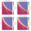 |
Fig. D.1. Heat map of the simulated completeness on the diagram of Ih and rs, h of halo models for the first two non-LAH sources (RID = 5479 and 22230). Left and right panels show completeness maps for halo only models and those for halo and continuum-like components models. Black stars and asterisks on the map indicate the halo parameter sets that have completeness values from 45% to 54% and those from 54% to 70%, respectively, while white large, middle-size, and small circles represent the parameter sets whose Lyα fluxes of the halo models are from 1 × 10⁻¹⁸ erg s−1 cm−2 to 2 × 10⁻¹⁸ erg s−1 cm−2, those from 4 × 10⁻¹⁸ erg s−1 cm−2 to 6 × 10⁻¹⁸ erg s−1 cm−2, and those from 1 × 10⁻¹⁷ erg s−1 cm−2 to 2 × 10⁻¹⁷ erg s−1 cm−2, respectively. (a) and (b): RID = 5479. The flux of the continuum-like component is f(Lyα) = 1.5 × 10⁻¹⁷ erg s−1 cm−2. |
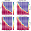 |
Fig. D.2. Same as Figure D.1, but for the last two non-LAH sources (RID = 23135 and 54891) (a) and (b): RID = 23135 with f(Lyα) = 3.7 × 10⁻¹⁹ erg s−1 cm−2. (c) and (d): RID = 54891 with f(Lyα) = 1.6 × 10⁻¹⁹ erg s−1 cm−2. |
Generally, there is a sharp transition between the parameter space with high completeness values in blue, and the parameter space with low completeness values in red, depending on Ih and rs, h (see the drastic change of colors near black stars in Figures D.1 and D.2). The halo tests for the non-LAH sources are complete when the halo fluxes are equal to or brighter than ≃4 × 10⁻¹⁸ erg s−1 cm−2 to 6 × 10⁻¹⁸ erg s−1 cm−2 in most of the parameter ranges. At a fixed halo flux range (see white circles with a given size), completeness decreases both when rs, h is too small and too large. Compact haloes with rs, h ≲ 1 − 3 kpc mostly cannot be detected due to the MUSE PSF and the method in which we only used r = rin − rCoG. We note that Leclercq et al. (2017) found compact haloes with rs, h = 2 − 3 kpc with shallower MUSE data without AO, because of the difference in the methods. We also would like to note that the re in UV is ≃0.5 − 1.7 kpc, which is relatively close to our limit. The halo only models and halo and continuum-like component models have similar distribution of completeness and median rCoG in most of the case. However, the completeness of the two cases are slightly different from each other when the values are low as seen in Fig. D.3 (lower than 70%; black asterisks). In particular, if a galaxy has a bright continuum-like Lyα component like RID = 5479, its extended emission can be hidden by the continuum-like component for some cases. The non-LAH, RID = 5479, has a ≃0.25 to 1 times lower completeness for the two-component model than that of the halo only model, when the only halo completeness is ≃50%−70% with relatively bright Ih (i.e., most of the cases with halo fluxes lower than 6 × 10⁻¹⁸ erg s−1 cm−2). However, a bright-continuum component can also help the halo detection by increasing the S/N required for the test, when Ih is low. The parameter space in which the completeness for both cases is different is narrow for RID = 5479, and the trend holds for both directions. We conclude that it does not cause a serious bias to our tests. With regard to rCoG, it is natural that the median value gets slightly higher for halo and continuum-like components models than halo only counterparts, since the continuum-like components can enhance the S/N on the outskirts. With the completeness obtained here, we give an overview of non-LAHs in Section 3.3.4, focusing on an object included in the UV-bright sample (RID = 5479), and closely look at the other sources below.
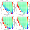 |
Fig. D.3. Heat map of the relative difference in the completeness for four non-LAHs on the diagram of Ih and rs, h of halo models. The relative difference in completeness is defined as ( |


D.2. RID = 22230
This object has a high confidence level of ZCONF = 2 for zs = 3.46 in the MXDF catalog and M1500 = −18.60. It shows a clear Lyα emission line on the 1D spectrum for  as shown in Figure 4 and has S/N(rin − rCoG) = 6.72 with
  . However, the SB profile at r ≥ rin is consistent with that of the MUSE PSF-convolved HST profile (continuum-like component), with p0 = 0.273, which is higher than the threshold of 0.05. The completeness simulations for RID = 22230 is shown in Figure D.1. For instance, the completeness decreases to ≃50% at rs, h = 4.5 kpc and Ih = 8.8 × 10⁻¹⁹ erg s−1 cm−2 arcsec−2.
On the radial SB profile shown in Figure 8, we can see an absorption-like dip at the top of the profile with surrounding emission. The dip could be created by the combination of Lyα absorption and spatially offset and anisotropic distribution of Lyα, which can be confirmed on the NB image by eye (Figure 4). The S/N of the extended flux (at r ≥ rin) would be higher if we only use angle-limited spatial pixels with a direction of the extended Lyα emission. If we could consider the SB profile at r ≤ rin, which is found to be different from the shape of the MUSE PSF-convolved HST profile by eye, we might be able to confirm a potential halo. Deeper and higher-spatial resolution data set than MXDF will help improve the test, but with the current data set and method, this object is classified as a non-LAH. This object is not included in the UV-bright sample and does not influence on our main conclusions, or could even support our main conclusions if it was classified as a LAH.
D.3. RID = 23135
This object has a confidence level of ZCONF = 1 for zs = 3.94 in the MXDF catalog and M1500 = −18.39. As discussed in Section 2.2, it has a faint but ORIGIN-detected Lyα emission line, which can be seen on the 1D spectrum for  in Figure 5. However, the object does not have a sufficient number of spectral slices with S/N > 1.5 at r = rin − rCoG that can be used to create the optimized NBs (see Section 3.2). As a consequence, it has a low S/N(rin − rCoG) (< 0) on the NB with
  . Therefore, it is clear that this object does not have a significant Lyα halo above the observational limit. The completeness simulations for RID = 23135 are shown in Figure D.2. For instance, the completeness decreases to ≃50% at rs, h = 4.9 kpc and Ih = 5.5 × 10⁻¹⁹ erg s−1 cm−2 arcsec−2.
We would like to note that the nondetection of a halo should not be a direct result of a wrong redshift (i.e., low ZCONF value). On the contrary, if it had a clear extended Lyα emission line, it could be a redshift indicator and raise the ZCONF value in the MXDF catalog. Since the UV magnitude is faint, this object is not included in the UV-bright sample. The Lyα halo fraction for the sample including all sources could be even higher, if we excluded this object.
D.4. RID = 54891
This object has a confidence level of ZCONF = 0 for zs = 2.94 and M1500 = −18.02. As discussed in Section 2.2, it does not have ORIGIN-detected lines but has a faint Lyα line (see the NB and SB profile in Figure 5). Similar to RID = 23135, the object does not have a sufficient number of spectral slices at r = rin − rCoG for an optimized NB (see Section 3.2;  ,
,  ), the S/N(rin − rCoG) on the NB is only 1.29. Therefore, it is clear that this object does not have a significant Lyα halo. The completeness simulations for RID = 54891 is shown in Figure D.2. For instance, the completeness decreases to ≃50% at rs, h = 6.3 kpc and Ih = 5.7 × 10⁻¹⁹ erg s−1 cm−2 arcsec−2. Since the UV magnitude is faint, this object is not included in the UV-bright sample.
All Tables
All Figures
|
Fig. 1. (a) Night sky spectrum as a function of observed wavelength. The black line shows the night sky spectrum with an arbitrary normalization. The light gray and dark shaded areas indicate the wavelength range of the AO gap and the wavelength range that is not used in this work, respectively. (b) 5σ noise surface brightness (SB) for the typical parameters for optimized NBs (see Sect. 3.2) as a function of redshift (black line). The light gray shaded area indicates the redshift range of the AO gap. (c) M1500 as a function of z for the sample. The large filled blue stars, large open blue stars, and small open blue stars indicate our sources with ZCONF = 2, 3, ZCONF = 1, and ZCONF = 0, respectively. The black dots show nonisolated galaxies (see Sect. 2.2). The black and green lines represent the F775W apparent magnitude cut, and the criteria for the UV-bright sample, respectively. |
| In the text | |
|
Fig. 2. Examples of the overview with two sources (a LAH RID = 4764 and a non-LAH RID = 5479). The first two rows show RID = 4764, while the last two rows show RID = 5479. (a) HST F775W image (rest-frame UV). The Rafelski’s ID (RID), the MUSE ID (MID), zs, ZCONF, and M1500 are indicated. The smaller and larger cyan circles present rin and rCoG (Sects. 3.1 and 3.2). (b) MUSE broad band image summed over the rest-frame UV range 1300–1800 Å. The image is smoothed with a 2D Gaussian filter with a standard deviation of 1 pixel. Spectroscopic redshifts of sources in the MXDF catalog in the minicube are indicated. (c) Optimized narrow band for Lyα with the neighboring object mask (purple areas). The image is smoothed with a 2D Gaussian filter with a standard deviation of 1 pixel. The white contours indicate a SB of 2 × 10⁻¹⁹ erg s−1 cm−2 arcsec−2. (d) 1D spectrum around the wavelength of Lyα extracted inside the target’s continuum-component mask. The spectra and the 1σ uncertainty are represented by the black line and the gray shaded area, respectively. The spectral width of the flux-maximized NB and the wavelength of Lyα converted from zs in the MXDF catalog are shown by the cyan dashed and solid lines, respectively. The spectral slices used to produce the optimized NB are indicated by the yellow shaded areas for sources with high S/N spectral slices at r = rin − rCoG. (e) 1D spectrum around the wavelength of Lyα extracted in r = rin − rCoG. (f) Radial SB profile of Lyα emission in log scale measured on the optimized NB image. The cyan shaded areas represent the radial range, r = rin − rCoG (see Sect. 3.3). The panel shows whether the source is an isolated or nonisolated object, and whether it is a Lyα halo (LAH) or non-LAH. All images are 15 arcsec each on a side. We note that the segmentation maps and the masks as well as zoomed-in HST F775W cutouts (4″ × 4″) are shown in Figs. C.1 and C.2. |
| In the text | |
|
Fig. 3. Overview of the first 7 sources in order of RID except for RID = 4764 and 5479. Each row shows a different object. Panels a–f: are the same as those of Fig. 2. Panel a: MID = 0 means that no MUSE ID is assigned in the MXDF catalog (i.e., ZCONF = 0). Panels d and e: the spectral slices used to produce the optimized NB are indicated by the yellow and orange shaded areas for sources with high S/N spectral slices at r = rin − rCoG and those with low S/N spectral slices at r = rin − rCoG, respectively (see Sect. 3.2). We note that the emission ring shown in the NB of RID = 7876 is caused by the mask for a source with extended emission. Since the ring is located outside rCoG, it does not affect our results. |
| In the text | |
|
Fig. 4. Same as Fig. 2, but for the middle 6 sources in order of RID. Each row shows a different object. Panels a–f: are the same as those of Fig. 2. We note that the emission rings shown in the NB of RID = 9944 is caused by the mask for a source with extended emission. Although the ring feature of RID = 9944 overlaps with r = rin − rCoG, this object is not included in the isolated sample (as well as RID = 7876), and the main conclusion about the Lyα halo fraction is not affected by the ring. |
| In the text | |
|
Fig. 5. Same as Fig. 2, but for the last 6 sources in order of RID. Each row shows a different object. Panels a–f: are the same as those of Fig. 2. |
| In the text | |
|
Fig. 6. Flowchart of the main part of our analysis with the four steps. The input data are indicated by the yellow rounded boxes at the top of the panel, while output data are indicated by the orange rounded boxes. The analysis and classification are shown by rectangles and diamonds, respectively. The obtained samples and parameters are presented by circles. The details of each step are provided in Sects. 2.3, 3.1–3.4. The numbers colored blue indicate the sections as a reference. The flux-maximized NBs were used to obtain the average SB profiles in Sect. 4.2.1. |
| In the text | |
|
Fig. 7. Results of the tests for the existence of a Lyα halo. Top panel: histogram of the flux S/Ns between r = rin and rCoG measured on the optimized Lyα NBs. Blue and gray histograms indicate galaxies above and below the threshold of S/N = 3 (black dashed line), Non-LAHs and LAH candidates, respectively. RID = 23135 has a negative S/N(rin − rCoG) and is counted as S/N(rin − rCoG) = 0 in the plot. Bottom panel: probability of the null hypothesis that the SB profile at r = rin − rCoG matches that of the target’s continuum-component profile vs. flux S/N between r = rin and rCoG for the LAH candidates. A black dashed line represents the border of LAHs and Non-LAHs. |
| In the text | |
|
Fig. 8. SB profiles from the optimized NBs with results of the Lyα halo tests. The gray, black, and blue points indicate the observed radial profiles, those used for the fit (with binning if needed), and the best-fit SB profiles of the PSF-convolved continuum-like component, respectively. The x error bars of the black points mark the range for each (combined) radial bin. The cyan shaded areas represent the radial ranges, r = rin − rCoG (see Sect. 3.3). The classification of LAH or non-LAH, the S/N of the flux at r = rin − rCoG, and the probability of the null hypothesis that the SB profile at r = rin − rCoG matches that of the target’s continuum-component profile are shown at the top of each panel. |
| In the text | |
|
Fig. 9. Halo parameter set (Ih and rs, h) showing 50% completeness for four non-LAH objects. We explored potential halo parameters for four non-LAHs by simulating completeness values of the halo tests. We assumed exponential profiles for the halo and continuum-like component models (h + c) shown by dashed lines and for halo only models (h) shown by solid lines (see Appendix D). The gray solid (black dashed), orange solid (red dashed), magenta solid (violet dashed), and cyan solid (blue dashed) lines represent RID = 5479, RID = 22230, RID = 23135, and RID = 54891 with halo only models (halo and continuum models), respectively. The black crosses indicate the halo parameters measured in Leclercq et al. (2017) for the common sources between Leclercq et al. (2017) and ours. |
| In the text | |
|
Fig. 10. Lyα halo fractions for the complete sample (gray bars) and the UV-bright sample (−20.0 ≤ M1500 ≤ −18.7; green bars). The XLAH for isolated sources and that for nonisolated sources are shown in the second and third columns, respectively. The black error bars indicate 68.3% confidence intervals. |
| In the text | |
|
Fig. 11. Typical Lyα SB profiles with cosmic dimming corrections scaled to z = 3.65. (a) The violet and blue solid lines show individual SB profiles of LAHs and non-LAHs, respectively. The black solid line and the gray shaded area indicate the mean SB profile of 17 LAHs and the 1σ uncertainty, respectively, while the red dashed line indicates the mean SB profile of 13 isolated LAHs. The black crosses represent the median profile of the 17 LAHs. The black dashed holizontal line shows the typical 1σ SB limit of the mean LAH stack. (b) The blue circles and cyan crosses show the median SB profile of stacked MUSE LAEs at z = 3 − 4 (Wisotzki et al. 2018, W18) and the same data multiplied by 1.85 to compare the profile shapes. |
| In the text | |
|
Fig. 12. Cumulative incidence rate of LAHs, dn/dz(LAH, M1500 ≤ M1500, 0), as a function of M1500, 0. The blue solid line and shading show the dn/dz(LAH, M1500 ≤ M1500, 0) at z ≃ 3.65 and the uncertainty, respectively. The uncertainty is propagated from the 1σ error of the XLAH for all the sources. The solid black and green lines indicate M1500 of the brightest source in our sample and the upper limit of M1500 for the UV-bright sample, respectively (the M1500 of the faintest source is −18 mag). The blue dashed thin and thick lines represent the dn/dz for DLAs and DLAs+sub-DLAs at z = 3.65 calculated from the best-fit formulae of the z evolution of absorbers in Zafar et al. (2013a). |
| In the text | |
|
Fig. 13. Cumulative incidence rate of LAHs, dn/dz(LAH, M1500 ≤ M1500, 0), as a function of M1500, 0 at different redshifts. The different colors (blue, green, and red) indicate different redshifts (z ≃ 3.65, 4.9, and 5.9 in panels a–c, respectively). The solid black vertical lines show the M1500 of the brightest and faintest sources in our sample. The green vertical line indicates the upper limit of M1500 for the UV-bright sample. (a) At z ≃ 3.65. The blue solid line and shading show the dn/dz(LAH, M1500 ≤ M1500, 0) and the uncertainty, respectively. The blue-dashed thin line, medium-thick line, and thick line represent the dn/dz for DLAs, DLAs+sub-DLAs, and DLAs+sub-DLAs+LLSs at the same redshift, respectively. (b) At z ≃ 4.9. (c) At z ≃ 5.9. |
| In the text | |
|
Fig. A.1. Photo-z vs. spec-z for 142 F775W < 27.5 mag sources. The blue stars, the red stars, and the magenta dots represent galaxies with ZCONF = 2 or 3, 1, and 0, respectively. The gray shaded areas indicate the spec-z outside the targeted redshift (z = 2.86 − 4.44) and the AO gap. The gray diagonal line and the black lines show the zp = zs relation, and zp = 2.86 and 4.44 lines, respectively. The photometric redshifts were estimated in Rafelski et al. (2015) with the Bayesian Photometric Redshift (BPZ) algorithm (Benitez 2000; Benitez et al. 2004; Coe et al. 2006). The error bars of zp show 95% upper and lower limits. |
| In the text | |
|
Fig. A.2. 1D spectra of the two non-LAEs with LAHs, RID = 4587 and 4764 discussed in Section 3.3.3, as examples of our inside spectra. The dark gray lines, the faint gray shaded areas, the black lines, and the magenta lines show the inner spectra, its 1σ uncertainties, the inner continuum spectra, and the best-fit power-law models for the continua, respectively. The blue and orange shaded areas indicate fluxes integrated for the Lyα emission and Lyα absorption measurements (the spectral windows, see Appendix A.3 for more details), respectively. We note that the Lyα absorption flux (more precisely, the upper limit of the absorption flux) was obtained by multiplying two to the integrated flux in the orange shaded spectral window. |
| In the text | |
|
Fig. A.3. Lyα NB centered at RID = 4838. The Lyα NB was extracted from the MXDF data cube with a wavelength range of 4935−4948 Å and a size of 10″ × 10″ by source inspector, which was used to visually inspect the MXDF sources. The color bar shows the flux with an arbitrary normalization. The filled pink and filled purple circles indicate a nonisolated galaxy in our sample and its neighbor, which is not included in our sample with a spec-z measurement, respectively. The black open circles show sources in the catalog of Rafelski et al. (2015). The cyan circle indicates a |
| In the text | |
|
Fig. A.4. Same as Figure A.3, but for RIDs = 7847, 7876, and 9944. The Lyα NB is centered at RID = 7876 with a wavelength range of 4838−4863 Å and a size of 10″ × 10″. The filled pink circles indicate three nonisolated galaxies in our sample. The purple open square shows a close MUSE-detected Lyα emitter without an HST counterpart. The purple open circle presents a potential neighbor, which does not have a spec-z but has a close photo-z. The black open circles show sources in the catalog of Rafelski et al. (2015). The cyan circles indicate |
| In the text | |
|
Fig. B.1. Examples of the difference in the radial SB profiles for four different settings of the continuum subtractions. The black and blue lines indicate the SB profiles for the original minicubes and the continuum-subtracted minicubes, respectively. The neighboring masks were applied for both. The cyan shaded areas indicate the radii outside the target’s continuum-component masks and inside the rCoG. Left column: RID = 4764, which has an artificial absorption trough with the general setting of a 200-pix (±100-pix) window. Right column: RID = 9863, which has a neighbor (at the radius shown by the magenta solid line) that cannot be eliminated only by the neighboring object mask. From top to bottom, each panel represents the settings: 1) 200-pix (±100-pix) window, 2) 200-pix (±100-pix) window + Lyα mask (±400 km s−1 around Lyα), 3) 100-pix (±50-pix) window + Lyα mask, and 4) 60-pix (±30-pix) window + Lyα mask, respectively. |
| In the text | |
|
Fig. C.1. HST cutouts, segmentation maps, and masks for the first 10 sources in order of RID. First column: 4″ × 4″ HST F775W cutout images. The purple dots and circles represent the positions of the UV-selected galaxy and rin, respectively. Second column: 4″ × 4″ cutouts of the HST segmentation map. The yellow and green regions indicate the areas in which the target and neighboring galaxies are detected on the HST images, respectively. The segmentation map gives the boundaries of the objects. The dark purple regions indicate the sky. Third column: target’s continuum-component masks (in the spatial resolution of MUSE, 15″ × 15″). The yellow and dark purple regions present the mask (the area of the main part of the galaxy) and the sky, respectively. The violet circles show rCoG. Fourth column: Neighboring object masks (neighbor mask; in the spatial resolution of MUSE, 15″ × 15″). The yellow and dark purple regions present the mask (the area of the main part of neighboring galaxies that have a bright continuum) and the sky, respectively. |
| In the text | |
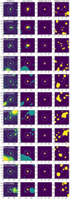 |
Fig. C.2. Same as Figure C.1, but for the last 11 sources in order of RID. |
| In the text | |
|
Fig. D.1. Heat map of the simulated completeness on the diagram of Ih and rs, h of halo models for the first two non-LAH sources (RID = 5479 and 22230). Left and right panels show completeness maps for halo only models and those for halo and continuum-like components models. Black stars and asterisks on the map indicate the halo parameter sets that have completeness values from 45% to 54% and those from 54% to 70%, respectively, while white large, middle-size, and small circles represent the parameter sets whose Lyα fluxes of the halo models are from 1 × 10⁻¹⁸ erg s−1 cm−2 to 2 × 10⁻¹⁸ erg s−1 cm−2, those from 4 × 10⁻¹⁸ erg s−1 cm−2 to 6 × 10⁻¹⁸ erg s−1 cm−2, and those from 1 × 10⁻¹⁷ erg s−1 cm−2 to 2 × 10⁻¹⁷ erg s−1 cm−2, respectively. (a) and (b): RID = 5479. The flux of the continuum-like component is f(Lyα) = 1.5 × 10⁻¹⁷ erg s−1 cm−2. |
| In the text | |
|
Fig. D.2. Same as Figure D.1, but for the last two non-LAH sources (RID = 23135 and 54891) (a) and (b): RID = 23135 with f(Lyα) = 3.7 × 10⁻¹⁹ erg s−1 cm−2. (c) and (d): RID = 54891 with f(Lyα) = 1.6 × 10⁻¹⁹ erg s−1 cm−2. |
| In the text | |
|
Fig. D.3. Heat map of the relative difference in the completeness for four non-LAHs on the diagram of Ih and rs, h of halo models. The relative difference in completeness is defined as ( |
| In the text | |
Current usage metrics show cumulative count of Article Views (full-text article views including HTML views, PDF and ePub downloads, according to the available data) and Abstracts Views on Vision4Press platform.
Data correspond to usage on the plateform after 2015. The current usage metrics is available 48-96 hours after online publication and is updated daily on week days.
Initial download of the metrics may take a while.