| Issue |
A&A
Volume 659, March 2022
|
|
|---|---|---|
| Article Number | A67 | |
| Number of page(s) | 43 | |
| Section | Interstellar and circumstellar matter | |
| DOI | https://doi.org/10.1051/0004-6361/202141790 | |
| Published online | 08 March 2022 | |
Chemical survey of Class I protostars with the IRAM-30 m★
1
INAF, Osservatorio Astrofisico di Arcetri,
Largo E. Fermi 5,
50125
Firenze,
Italy
e-mail: This email address is being protected from spambots. You need JavaScript enabled to view it.
2
Università degli Studi di Firenze, Dipartimento di Fisica e Astronomia,
Via G. Sansone 1,
50019
Sesto Fiorentino,
Italy
3
Univ. Grenoble Alpes, CNRS, Institut de Planétologie et d’Astrophysique de Grenoble (IPAG),
38000
Grenoble,
France
4
École doctorale de Physique, Université Grenoble Alpes,
110 rue de la Chimie,
38400
Saint-Martin-d’Hères,
France
5
Institut de Radioastronomie Millimétrique,
38406
Saint-Martin d’Hères,
France
Received:
14
July
2021
Accepted:
10
November
2021
Abstract
Context. Class I protostars are a bridge between Class 0 protostars (≤105 yr old), and Class II (≥106 yr) protoplanetary disks. Recent studies show gaps and rings in the dust distribution of disks younger than 1 Myr, suggesting that planet formation may start already at the Class I stage. To understand what chemistry planets will inherit, it is crucial to characterize the chemistry of Class I sources and to investigate how chemical complexity evolves from Class 0 protostars to protoplanetary disks.
Aims. There are two goals: (i) to perform a census of the molecular complexity in a sample of four Class I protostars, and (ii) to compare the data with the chemical compositions of earlier and later phases of the Sun-like star formation process.
Methods. We performed IRAM-30 m observations at 1.3 mm towards four Class I objects (L1489-IRS, B5-IRS1, L1455-IRS1, and L1551-IRS5). The column densities of the detected species were derived assuming local thermodynamic equilibrium (LTE) or large velocity gradients (LVGs).
Results. We detected 27 species: C-chains, N-bearing species, S-bearing species, Si-bearing species, deuterated molecules, and interstellar complex organic molecules (iCOMs; CH3OH, CH3CN, CH3CHO, and HCOOCH3). Among the members of the observed sample, L1551-IRS5 is the most chemically rich source. Different spectral profiles are observed: (i) narrow lines (~1 km s−1) towards all the sources, (ii) broader lines (~4 km s−1) towards L1551-IRS5, and (iii) line wings due to outflows (in B5-IRS1, L1455-IRS1, and L1551-IRS5). Narrow c-C3H2 emission originates from the envelope with temperatures of 5–25 K and sizes of ~2′′−10′′. The iCOMs in L1551-IRS5 reveal the occurrence of hot corino chemistry, with CH3OH and CH3CN lines originating from a compact (~0.′′15) and warm (T > 50 K) region. Finally, OCS and H2S seem to probe the circumbinary disks in the L1455-IRS1 and L1551-IRS5 binary systems. The deuteration in terms of elemental D/H in the molecular envelopes is: ~10−70% (D2CO/H2CO), ~5−15% (HDCS/H2CS), and ~1−23% (CH2DOH/CH3OH). For the L1551-IRS5 hot corino we derive D/H ~2% (CH2DOH/CH3OH).
Conclusions. Carbon chain chemistry in extended envelopes is revealed towards all the sources. In addition, B5-IRS1, L1455-IRS1, and L1551-IRS5 show a low-excitation methanol line that is narrow and centered at systemic velocity, suggesting an origin from an extended structure, plausibly UV-illuminated. The abundance ratios of CH3CN, CH3CHO, and HCOOCH3 with respect to CH3OH measured towards the L1551-IRS5 hot corino are comparable to that estimated at earlier stages (prestellar cores, Class 0 protostars), and to that found in comets. The deuteration in our sample is also consistent with the values estimated for sources at earlier stages. These findings support the inheritance scenario from prestellar cores to the Class I phase when planets start forming.
Key words: astrochemistry / stars: formation / ISM: molecules
A copy of the reduced spectra is only available at the CDS via anonymous ftp to cdsarc.u-strasbg.fr (130.79.128.5) or via http://cdsarc.u-strasbg.fr/viz-bin/cat/J/A+A/659/A67
© ESO 2022
1 Introduction
After just two decades from the first discovered exoplanet (Wolszczan & Frail 1992) the field of exoplanets has reached maturity (e.g., Doyle et al. 2011). The two most striking results have been the almost ubiquitous presence of planetary systems around main sequence stars and the overwhelming diversity of system architectures. Both of these findings strongly motivate the quests of the origins of such diversity. The question is now what the next step should be. The future is enlightened by a breakthrough discovery: planets already start to form during the Class I phase (≥105 yr) (e.g., Sheehan & Eisner 2017; Fedele et al. 2018). It is necessary to investigate the physical and chemical properties of the first stages of a Sun-like star, and to compare them with what has been found in our Solar System to reveal the chemical origin of planets.
Class I protostars, with a typical age of 105 yr are a bridge between Class 0 protostars (~104 yr), where the bulk of the material that forms the protostar is still in the envelope and the Class II protoplanetary disks (106 yr). Class I sources have recently begun to be chemically characterized through spectral surveys at millimeter wavelengths to search for interstellar complex organic molecules, small organics, and deuterated species (Öberg et al. 2014; Bergner et al. 2017, 2019; Bianchi et al. 2017a, 2019a, 2020; Le Gal et al. 2020). Therefore, we are still far from concluding whether Class I protostars are also a bridge from a chemical point of view.
Interstellar complex organic molecules (iCOMs1), which are C-bearing molecules containing at least six atoms (Herbst & van Dishoeck 2009; Ceccarelli et al. 2017), are the building blocks of pre-biotic molecules. Hence, it is very significant to understand how iCOM abundances vary in the evolutionary path from prestellar core to Solar System small bodies. Hot corinos around Class 0 protostars are chemically enriched due to the release of molecules, including iCOMs, from the surfaces of dust grains heated by the protostar up to temperatures greater than 100 K (Ceccarelli et al. 2007). They have been well studied so far (e.g., Bottinelli et al. 2007; Codella et al. 2016; Jørgensen et al. 2016, 2020; Belloche et al. 2020; Yang et al. 2021, and references therein). Recently, ALMA observations also started to reveal the chemical content of protoplanetary disks (PPDs) with the detection of a few iCOMs (Öberg et al. 2015; Walsh et al. 2016; Bergner et al. 2018; Favre et al. 2018; Lee et al. 2019b; Podio et al. 2020; Booth et al. 2021). However, to our knowledge, there are only a few studies on the detection of a hot corino towards Class I protostars (Bergner et al. 2019; Bianchi et al. 2019b, 2020; Yang et al. 2021), and very little has been done in terms of comparison of the chemical complexity at the different stages along the star formation process from prestellar cores to comets (see, e.g., Bianchi et al. 2019b; Drozdovskaya et al. 2019, 2021; Podio et al. 2020; Booth et al. 2021). Conversely, protostars can also be enriched with carbon-chain molecules and are called warm carbon-chain chemistry (WCCC) sources (e.g., Sakai et al. 2008, 2010; Sakai & Yamamoto 2013), which are known to lack iCOMs. The origin of the chemical diversity is still unknown.
Deuterium-bearing species are also a powerful key to investigating the chemical evolution from prestellar cores to our Solar System (Ceccarelli et al. 2014). The deuteration of molecules (i.e., the enhancement of the D/H abundance ratio in a given molecule with respect to the cosmic elemental deuterium abundance) (D/H = 1.6 × 10⁻⁵, Linsky 2007) occurs in cold and dense environments, such as prestellar cores, and is stored onto dust mantles. Deuterated molecules are then released into the gas phase when either the temperature is high enough to evaporate the grain mantles (e.g., Ceccarelli et al. 2007; Parise et al. 2004, 2006) or when protostellar shocks sputter the grains (Codella et al. 2012). Therefore, the D/H ratios are believed to be “fossils” of the solar-like star forming process (e.g., Taquet et al. 2012; Jaber Al-Edhari et al. 2017). In this perspective, several prestellar cores and Class 0 protostars are studied by focusing on the deuterium fractionation of H2CO, H2CS, and CH3OH (e.g., Bacmann et al. 2003; Marcelino et al. 2005; Bizzocchi et al. 2014; Vastel et al. 2018; Parise et al. 2006; Bianchi et al. 2017b; Drozdovskaya et al. 2018; Manigand et al. 2020, and references therein). On the other hand, there is only one Class I protostar for which the deuterium fractionation of these species has been measured, SVS13-A (Bianchi et al. 2017a, 2019a).
In this context we present a chemical survey of four Class I protostars by examining their molecular complexity, molecular deuteration, and their physical characterization. The paper is organized as follows: In Sect. 2 we present the source sample; in Sect. 3 we show the observations; in Sect. 4we present the analysis of the detected molecular lines; in Sect. 5.1 we discuss the molecular diversity among the targeted protostars, depending on the profiles, abundance, and deuteration of the detected molecules, and we put it in the context of the sources evolutionary stage; in Sect. 6 we summarize our findings.
Observed sample of Class I sources.
2 The sample
Four Class I (see Table 1) sources have been selected according to the following criteria: (1) They are located in two different nearby star forming regions, Taurus at d = 141 pc and Perseus at d = 294 pc (Zucker et al. 2019). (2) They are classified as Class I sources, having a bolometric temperature Tbol > 70 K (Chen et al. 1995; Andre et al. 2000). (3) They are associated with emission in methanol lines with upper level energies, Eup, up to ~ 80 K detected with IRAM-30 m and ALMA observations suggesting the occurrence of a hot corino activity. The exception is L1489-IRS, where only methanol lines with low upper level energies were detected (Eup ≤ 12 K), pointing to emission from the surrounding envelope (e.g., Öberg et al. 2014; Graninger et al. 2016; Bianchi et al. 2020).
We ordered the sources in the same way that we use in the table and throughout the paper (from the chemically poorest to the chemically richest). The coordinates of the sources and the distances, systemic velocities, and bolometric luminosities are presented inTable 1.
2.1 L1489-IRS
L1489 IRS (also known as IRAS 04016+2610) is located in the Taurus star forming region. The bolometric luminosity of the source is 3.5 L⊙ (Green et al. 2013). Interferometric observations of C18O, 13CO, SO, HCO+, and HCN show infalling flows (Hogerheijde 2001; Yen et al. 2014), a faint bipolar outflow (Myers et al. 1988; Hogerheijde et al. 1998; Yen et al. 2014), and a large Keplerian disk with r ~ 700 au (Yen et al. 2014). IRAM-30 m observations reveal emission from several molecules (sulfur- and nitrogen- bearing species, molecular ions, and deuterated molecules) (e.g., Law et al. 2018; Le Gal et al. 2020, and references therein). Öberg et al. (2014) detected CH3OH lines with Eup ~ 6–12 K.
2.2 B5-IRS1
B5-IRS1 (Barnard 5 IRS1, also known as IRAS 03445+3242 and Per-emb 53) is located in the B5 region of the Perseus molecular cloud. It has a bolometric luminosity of 5 L⊙ (Beichman et al. 1984; Evans et al. 2009; Pineda et al. 2011), and it is embedded in a core within a filamentary structure observed in NH3 emission. In addition, Yu et al. (1999) reported a bright jet using H2 and Hα emission at optical–near-infrared wavelengths. A bipolar outflow has also been revealed (e.g., Bally et al. 1996; Yu et al. 1999; Zapata et al. 2014, and references therein). More specifically, Zapata et al. (2014) resolved the outflow structure by using Submillimeter Array observations of CO emission. Their images showed a spider-like structure, with a high-velocity outflow component nested inside a slower wide-angle component. Narrow emission (0.8 km s−1) in CH3OH, in CH3CN and, tentatively, in CH3CHO, has been detected using the IRAM-30 m telescope (Öberg et al. 2014). In addition, emission from nitrogen- and sulfur-bearing molecules and from carbon chains has been detected (Öberg et al. 2014; Law et al. 2018). Yang et al. (2021) has detected CH3OH emission using ALMA observations.
2.3 L1455-IRS1
L1455-IRS1 (also known as IRAS 03245+3002 and Per-emb 17) is located in the Perseus molecular cloud. This protostar is one of the brightest Class I sources in the L1455 region with a bolometric luminosity of 3.6 L⊙ (Dunham et al. 2013). Goldsmith et al. (1984) and Chou et al. (2016) showed that the source is associated with a Keplerian disk (r < 200 au) and drives a high-velocity outflow mapped in CO and C18O out to distances of ~6000 au. This source is also associated with three knots detected in H2 lines at near-infrared wavelengths (Davis et al. 1997), which are located symmetrically with respect to the driving source in agreement with the collimated outflow structure imaged by Curtis et al. (2010). IRAM-30 m studies show that the source is associated with emission of both carbon chains and complex organic molecules: Graninger et al. (2016) detected CH3OH lines with Eup up to ~30 K; Law et al. (2018) reported several S-bearing and N-bearing species; Bergner et al. (2017) detected CH3CHO at low Eup ~ 15 K as well as nitrogen-bearing molecules. ALMA and VLA observations show that L1455-IRS1 is a binary system (Tobin et al. 2018; Yang et al. 2021): Tobin et al. (2018) reported the surrounding circumbinary disks around the two sources and an elongated outflow structure. Using ALMA, Yang et al. (2021) reported a rich molecular complexity detecting iCOMs such as CH3OH, CH2DOH, HCOOCH3, CH3OCH3, NH2CHO, CH3CN, and CH2DCN.
2.4 L1551-IRS5
L1551-IRS5 is located in the Taurus star forming region and is classified as a Class I protostar (Adams et al. 1987; Looney et al. 1997) and as a FU Ori-like object (Connelley & Reipurth 2018) with bolometric luminosity between 30 and 40 L⊙ (Liseau et al. 2005). L1551-IRS5 is a binary system as shown by VLA (Bieging & Cohen 1985) and BIMA observations (Looney et al. 1997) and consists of a northern component of 0.8 M⊙ and a southern component of 0.3 M⊙ (Liseau et al. 2005), enclosed by a circumbinary disk (Cruz-Sáenz de Miera et al. 2019; Takakuwa et al. 2020). Both protostars drive jets as showed by VLA observations in the continuum image (Rodríguez et al. 2003). In addition, a recent ALMA study showed that the two circumstellar disks are associated with the two binary components, and are detected in CO and several S-bearing species (Takakuwa et al. 2020). ALMA observations also allowed the systemic velocities of the southern and northern components to be constrained as +4.5 km s−1 and +7.5 km s−1, respectively (Bianchi et al. 2020). They revealed a hot corino associated with the northern protostar thanks to the CH3OH, HCOOCH3, and CH3CH2OH emission lines.
Observational IRAM-30 m settings.
3 Observations
Observations were carried out at the IRAM-30 m telescope located on Pico Veleta, Spain, during several sessions in July 2018 and May 2019. All sources were observed in band E2 (1.3 mm) in order to minimize beam dilution. To maximize the number of iCOMs and deuterated lines, the frequency ranges at 214.5–222.2 GHz and 230.2–238.0 GHz were selected with the Eight MIxer Receivers (EMIR) and the FTS200 backend, in wobbler switching mode. The spectral resolution is 0.2 MHz, corresponding to ~0.26 km s−1. In order to increase the S/N, the spectral resolution of the weakest lines was degraded up to ~1.0 km s−1. Precipitable water vapor (pwv) is ~3–5 mm. We estimate, using the W3(OH), 2251+158, 0430+052, and 0316+413 sources, the calibration uncertainty to be ~20%, while the error on pointing is ≤3′′. The half power beam width (HPBW) of the telescope varies from ~11′′ (at 214 GHz) to ~10′′ (at 238 GHz). This corresponds to ~1500 au for L1489-IRS and L1551-IRS5 and ~3000 au for B5-IRS1 and L1455-IRS1.
The GILDAS-CLASS2 package was used to perform the data reduction. Antenna temperature values (TA) were converted to main beam temperature values (TMB), according to beam efficiency of 0.60 and forward efficiency of 0.93 given in the IRAM-30 m website3. A summary of the observing settings is reported in Table 2, which reports system temperature, on-source observing time, spectral resolution, and HPBW. The average root mean square (rms) noise in the 0.26 km s−1 channel is ~10 mK (in TMB scale).
4 Results
4.1 Line Identification
We analyzed the 1.3 mm spectra obtained for the four Class I sources presented in Sect. 2 and searched for molecular emission. For the line identification we used the JPL4 and CDMS5 spectral catalogues. The lines were identified by fitting the profile with a Gaussian function in GILDAS-CLASS, which allowed us to retrieve the integrated line intensity, Iint; the line full width at half maximum, FWHM; and the intensity and velocity of the line peak, Tpeak and Vpeak.
We claim a line detection if the following three criteria are fulfilled: (1) the integrated intensity (Iint) is above 3σ (i.e., the line is detected with a S/N higher than 3); (2) the line peaks at |Vpeak − Vsys| < 0.6 km s−1, where Vsys is the source systemic velocity; (3) the line widths of different transitions due the same species are the same within the uncertainties. The results of the local thermodynamic equilibrium (LTE) and non-LTE analysis (see below) are used as an a posteriori check to spot false identifications. Diatomic and triatomic molecules (such as CO, CS, DCN) are identified even if only one line is detected. The identification of larger molecules (≥ 4 atoms) is done by verifying that in the observed frequency range the detected line(s) of one molecular species are expected to be the brightest one(s) assuming the typical conditions of protostellar regions, and by performing a careful comparison with the 1–3 mm unbiased spectral survey ASAI of chemical rich Class 0 and I sources (Lefloch et al. 2018). Future observations over a wider frequency range would be instructive.
The detected lines are shown in Figs. A.1–A.4. Tables A.1–A.4 report the spectral line parameters as well as the results of the Gaussian fit for all the detected lines, namely frequency (ν), telescope half power beam width (HPBW), upper level energy (Eup), line strength (Sμ2), rms noise, All abbreviations and acronyms (and instrument and program names when appropriate) must be introduced at first use; the abbreviation should then be used consistently. Please check throughout. channel width (δV), peak temperature (Tpeak), line peak velocity (Vpeak), FWHM, velocity integrated line intensity (Iint), and spectralcatalogues used.
For the transitions associated with multiple hyperfine components, we fit the spectral patterns taking these components into account. In this case, the fit provides, again, estimates of Vpeak, the FWHM line width, as well as the sum of the line opacities. The results, which are obtained with the CLASS tool, are reported in Table 3. Most of the species are optically thin (τ ≪ 1), while DCN, 13CS, 13CN, N2D+, and C15N are moderately optically thick (τ ~ 1–4). The J = 2–1 transition of CO, 13CO, and C18O has been observed towards all the sources.
In addition, taking into account all the sources, we detected the following species (see Tables A.1–A.4):
C-chains (c-C3H, c-C3H2, and CH3CCH);
iCOMs (CH3OH, CH3CN, CH3CHO, and HCOOCH3);
N-bearing species (13CN, C15N, and HNCO);
S-bearing molecules (SO, 34SO, SO2, 13CS, OCS, O13CS, CCS, H2S, H2CS, and H2C33S);
Si-bearing species (SiO);
Deuterated molecules (DCO+, N2D+, CCD, DCN, HDCS, D2CO, and CH2DOH).
Figure 1 shows the 1.3 mm spectra of the four observed Class I protostars. The labels indicate the brightest detected lines towards the four sources, in particular CO and the brightest line for each category of molecules listed above. More specifically: c-C3H2 for C-chains, CH3OH for iCOMs, 13CN for N-bearing species, SO for S-bearing molecules, SiO for Si-bearing species, and DCO+ for deuterated isotopologues. The sources are ordered by increasing number of line detections (L1489-IRS, B5-IRS1, L1455-IRS1, and L1551-IRS5, respectively). Figure 2 summarizes the number of detected lines per species and per source showing main isotopologues of iCOMs, C-chains, and S-bearing molecules. As listed in Table 4, we detected 17 transitions due to 10 species in L1489-IRS, 29 transitions due to 15 species in B5-IRS1, and 36 transitions due to 21 species in L1455-IRS1.L1551-IRS5 has the richest spectra in these observations in terms of detected number of molecules with 75 transitions due to 27 species.
To summarize, CO, SO, and H2CO emission has been detected in all four of the sources; the C-chain c-C3H2 and several deuterated species (DCO+, DCN, CCD, and D2CO) have been revealed towards all the targets; CH3OH and CH2DOH have been detected in all the sources apart from L1489-IRS; L1455-IRS1 and L1551-IRS5 show H2S, OCS, and H2CS emission; SiO emission has been observed only towards L1455-IRS1; CH3CN and CH3CHO have been detected towards L1551-IRS5 supporting the occurrence of a hot corino, first detected through CH3OH and HCOOCH3 emission by Bianchi et al. (2020).
The observed chemical differentiation will be discussed in Sect. 5.1, in light of gas properties and molecular column densities inferred through the line analysis presented in the following subsections.
Results of the spectral fit of the hyperfine components performed using the GILDAS-CLASS tool: sum of the opacities, line width, and peak velocity.
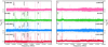 |
Fig. 1 Spectra observed in the 214 500–222 200 MHz and 230 200–238 000 MHz range towards L1489–IRS, B5–IRS1, L1455–IRS1, and L1551–IRS5, ordered from top to bottom according to the number of detected lines (see Table 4). Labels of selected detected species (see Sect. 4.1, Figs. A.1–A.4, and Tables A.1–A.4) are reported. |
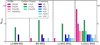 |
Fig. 2 Histogram of the numbers of detected lines for iCOMs (pink), C-chains (green), S-bearing molecules (blue) for the four protostars in our sample (ordered by increasing number of detected species). |
4.2 Constraints on line optical depth
Given the large number of isotopologues (12 lines due to five species) detected in the present survey, we derive constraints on the opacity of the detected emission lines by assuming interstellar isotopic ratios. Figures A.5 and A.6 show the 12C/13C from J = 2–1 profiles of 12CO, 13CO, and C18O. The spectraof the rarer isotopologues are scaled assuming the isotopic ratios of 12C/13C = 77 and 16O/18O = 560 (Milam et al. 2005). The line emission at velocities close to the systemic value are affected by absorption. In addition, in the case of L1551-IRS5, there is also foreground emission producing an absorbing dip at blueshifted velocity of ~8 km s−1. On the other hand, the line intensities at the highest velocities are consistent with the isotopic ratios, indicating optically thin emission (τ ≤ 0.1).
For SO 65 –54, we compare the 32SO and 34SO line emission towards B5-IRS1 and L1551-IRS5. The line ratio is ~12–20; assuming an isotopic ratio 32S/34S = 22 (Wilson & Rood 1994), this leads to an opacity of 32SO 65 –54 of ~ 1.
We also estimate the opacity of the H2C32S 71,7 –61,6 emission by comparison with H2C33S 71,7 –61,6. Assuming an isotopic ratio 32S/33S = 138 (Wilson & Rood 1994), the measured line ratio of ~4 implies optically thick H2C32S emission (τ ≃ 35). Similarly, the opacity of OCS J = 19–18 emission is inferred from the line ratio of O12CS 19− 18 to O13 CS 19− 18, assuming 12C/13C = 77 (Milam et al. 2005). We find that the opacity of the O12 CS 19–18 line isaround 20.
Detected molecular species in the observed Class I sources.
4.3 LTE analysis
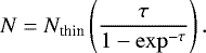
For the molecules detected in at least two lines, we used the standard rotational diagram (RD) approach to determine the rotational temperature and the column density (Goldsmith & Langer 1999). We assumed optically thin line emission and LTE conditions. For the species for which we estimated optically thick emission (see Sect. 4.2) we applied an a posteriori correction to the estimated column density, as explained below. The upper level column density of the u → l transition was calculated using
 (1)
(1)
Here Nu is the upper level column density (cm−2), k and h are respectively the Boltzmann (erg K−1) and Planck (erg s) constants, Aul is the Einstein coefficient (s−1), ηbf 6 is the beam-filling factor, c is speed of the light (cm s−1), ν is the rest frequency (GHz), and ∫ TmbdV is the integrated emission (K km s−1) in main beam temperature scale. As the beam is roughly the same for all the observed transitions (10′′–11′′), and because we do not know a priori the source size, we do not correct the line intensities for the beam filling factor (i.e., ηbf = 1 in Eq. (1)). Hence, the derived Nu is the beam-averaged column density.
According to the LTE assumption, we can describe Ntot and Trot with the following equation:
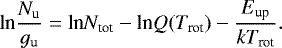 (2)
(2)
Here Ntot is the total beam-averaged column density of the molecule, gup is the degeneracy of the upper level, Eup is the energy of the upper level, and Q(Trot) is the partition function depending on the rotational temperature Trot.
The Trot and beam-averaged Ntot (cm−2) values derived from the rotational diagram analysis for each molecule and for each source are listed in Table 5. In the table we also report the number of lines used for the RD, and the interval of upper level energies (K) of the detectedlines. The rotational diagrams for the examined molecules towards the four protostars are shown in Figs. B.1–B.4. In Sect. 4.5 we apply the non-LTE analysis in the LVG approximation for the molecules where more than three lines are detected and collisional rates are available. In these cases we derived the source size, hence the column densities are source-averaged. In the case of H2CS and OCS, whose emission is optically thick, we correct the column density values (see Table B.4) for the optical depth derived in Sect. 4.2 using the following equation:
 (3)
(3)
In L1489-IRS, B5-IRS1, and L1455-IRS1 the rotational temperatures of all the analyzed species are quite low, less than about 30 K, with the exception of H2CO in L1455-IRS1 for which wefind Trot = (68 ± 25) K. On the other hand, L1551-IRS5 is associated with iCOMs emission for which we find higher Trot, up to (148 ± 30) K. The beam-averaged column densities (as derived using the RD analysis) are in the range of 1011 –1013 cm−2, with the exception of SO and CH3OH for which we find Ntot of a few 1014 cm−2.
4.4 Line profiles
The observed line profiles are very complex and differ from source to source (see Figs. A.1– A.4), with high-velocity wings, secondary peaks, and different line widths. The CO and 13CO profiles are affected by deep absorption at systemic velocity and by absorption features due to CO molecules along the line of sight. Broad line wings up to about ±10 km s−1 with respect to Vsys have been detected in CO, 13CO, C18O, and in other species. Lines with FWHM ~ 1–2 km s−1, centered at Vsys, are expected to be emitted by the molecular envelope, while iCOMs emission with ~4 km s−1 line width plausibly trace the compact (less than 1′′) hot corino. A special case is represented by L1551-IRS5, where the multi-peak profiles allow us to disentangle the emission coming from both the envelope and the hot corino (see Sect. 5.2).
By selecting different velocity ranges, we were able to derive the column densities of the different kinematical components: the envelope (Sect. 4.4.1), the outflow (Sect. 4.4.2), and the hot corino (Sect. 4.4.3). In some cases, the need to have S/N of at least 3 (for the intensities in selected velocity ranges) forced us to use fewer lines and, as a consequence, to assume the rotational temperature derived from other species that trace the same component and for which we were able to obtain a reliable RD. As described in the next sections, we assumed the following: (i) Trot = 20–35 K for the envelope (from c-C3H2), (ii) Trot = 50–70 K for the outflows (from SO and H2CO), and (iii) Trot = 60–150 K for the L1551 hot corino (from CH3OH).
Number of detected lines (S∕N ≥ 3), range of upper level energies of the detected transitions, temperatures (K), and beam-averaged column densities (cm−2) derived from the rotational diagram analysis.
4.4.1 Envelope tracers
Since c-C3H2 is detected in all the sources and shows a well-defined Gaussian profile with FWHM ~ 1.5 km s−1, we used this species as a reference to define the temperature range for the envelope (Trot = 20–35 K). These temperatures have been adopted to estimate the column densities of species observed through one emission line only. For lines (due to other species) broader than 1.5 km s−1, we integrated the line intensity in the velocity range ±1 km s−1 around Vsys to disentangle the envelope component. Tables B.1–B.4 report the derived Trot and Ntot values obtained for the envelope component. Source averaged column densities can be obtained from beam-averaged column densities by applying the filling factors reported for c-C3H2 in Table 6. Finally, for L1551-IRS5 we had the possibility to apply the RD approach for both ortho and para D2CO species separately. Figure B.4 shows that the present data do not allow us to reveal the expected o/p statistical values (3:1), likely due to poor statistics and to the low S/N value of the spectra.
4.4.2 Outflow tracers
We detected line wings up to approximately ±10 km s−1 with respect to the systemic velocity for a large number of species in addition to the CO isotopologues: H2CO, SO, SO2, 13CS, DCN, H2S, DCO+, and H2CS. This high-velocity emission (see, e.g., Figs. A.2–A.4) is plausibly due to the outflow motions, and is detected in all the sources. On the other hand we do not see high-velocity outflow motion in the line profiles of L1489-IRS.
In order to analyze the outflow contribution, we used the emission integrated at high velocities in the residual spectra after subtraction of the brighter emission at systemic velocity due to the envelope fit with a Gaussian (with FWHM ~ 1.5 km s−1 consistent with envelope emission). Rotational temperatures and column densities derived for the high-velocity outflow components are reported in Tables B.2–B.4. For the species where the rotational diagram analysis cannot be performed, because only one line is detected, we derived the column densities by assuming Trot ~ 50–70 K, following what was found using H2CO.
4.4.3 Hot corino tracers
Only L1551-IRS5 shows emission lines with line widths of ~4 km s−1 due to several iCOMs: CH3OH, CH3CN, CH3CHO, and HCOOCH3. This points to the presence of a hot corino, in agreement with the very recent ALMA results by Bianchi et al. (2020) who imaged a hot corino using CH3OH, CH2DOH, HCOOCH3, and t-CH3CH2OH. The chemical richness looks to be predominantly associated with the northern component of the L1551-IRS5 binary system, peaking at +7.5 km s−1. The L1551-IRS5 system, including both a hot corino and an envelope, is discussed in Sect. 5.2. In light of these findings, we derived the integrated emissions due to the hot corino also for OCS, O13 CS, and H2S, which show line widths larger than 4 km s−1, but with a well-defined emission peak at +7.5 km s−1. In addition, OCS and H2S show a broad emission (larger than 4 km s−1) also in L1455-IRS1, where methanol lines are narrow (FWHM = 1.6 km s−1). To be coherent with the L1551-IRS5 analysis we assumed a high temperature for the gas emitting OCS and H2S in L1455-IRS1, as was done for L1551-IRS5. The origin of the OCS and H2S emission is discussed in detail in Sect. 5.1.
We integrated the line intensities ±2 km s−1 around the hot corino velocity. The derived Trot and column densities derived using the RD approach are listed in Tables B.4. Rotational temperatures lie between 42 and 148 K, while beam-averaged column densities are ~1012–1014 cm−2. For species for which only a single transition is detected, we assumed Trot = 60–150 K and we derived column densities. Source averaged column densities can be obtained from beam-averaged column densities by applying the filling factors reported for CH3OH and CH3CN in Table 6.
Source-averaged molecular column density (Ntot), gas physical conditions (temperature, Tkin, and density, nH_2), source size inferred from the LVG analysis, and beam-filling factor (ηbf) of c-C3H2, CH3OH, and CH3CN lines towards the four protostars in our sample (L1489-IRS, B5-IRS1, L1455-IRS1, and L1551-IRS5).
4.5 Non-LTE large velocity gradient analysis
In order to derive the physical parameters of the emitting gas and the molecule column densities, we compare the line intensity measured in c-C3H2 (L1489-IRS, B5-IRS1, L1455-IRS1, and L1551-IRS5), CH3OH and CH3CN (L1551-IRS5) with the values predicted by the non-LTE LVG code grelvg (Ceccarelli et al. 2003). We compute the line intensities for a grid of molecular column densities, Nx; gas densities,  ; and temperatures, Tkin. Then the predicted line intensities are compared with the observed ones to determine the best fit (i.e., the values of Nx,
  , Tkin) and the source size θ, which gives the minimum χ2.
We carried out the non-LTE analysis only for three species (c-C3H2, CH3OH, and CH3CN) based on the following criteria: (1) at least four transitions have been detected, (2) the detected transitions cover a significant range of upper level energies, and (3) collisional coefficients are available in the literature. For c-C3H2, we used the collisional coefficients with He, computed by Chandra & Kegel (2000) and provided by the BASECOL database (Dubernet et al. 2013); for CH3OH, we used the collisional coefficients of both A and E transitions with para-H2, computed by Rabli & Flower (2010) and provided by the BASECOL database (Dubernet et al. 2013). For CH3CN, we used the H2 collisional coefficients by Green (1986), provided by the LAMDA database (Schöier et al. 2005).
When computing the line intensities with grelvg we assumed the following: (1) spherical geometry to compute the line escape probability (de Jong et al. 1980); (2) a A-CH3OH/E-CH3OH ratio equal to 1; (3) the ortho-H2/para-H2 ratio equal to 3; (4) a line width of 1 km s−1 for c-C3H2, 3 km s−1 for CH3OH, and 2.5 km s−1 for CH3CN (as derived from our observations). For CH3OH and CH3CN we used the integrated line intensities for the hot corino component described in Sect. 4.4.3. The uncertainties on the line integrated intensities, due to the error on calibration and the error on the Gaussian fit, amount to 30% of the observed intensities.
In the next subsections we describe the results obtained by applying the LVG analysis for each species. Table 6 summarizes the results of the LVG analysis by showing the number of lines, the range of upper level energy used for the analysis, kinetic temperatures, total column densities, H2 densities, and the source size of the species that reproduces the observations within a 1σ confidence level. From the estimated source size we also derive the beam filling factor of the emitting species, ηbf, reported in the last column of Table 6. Figure 3 shows the ranges of temperature, Tkin, and H2 density,  , obtained from the analysis of the CH3OH and CH3CN emission towards L1551-IRS5.
Finally, Fig. 4 shows the ratio between the observed overpredicted line intensities as a function of upper level energy of the transition.
 |
Fig. 3 Result of the LVG analysis for L1551-IRS5. The inferred range of gas density and temperature are summarized in Table 6. χ2 contour plots as a function of the gas density and temperature. The green and pink contours show the 1σ confidence level for CH3OH and CH3CN, respectively, for representative value of N(CH3OH) = 5 × 1018 cm−2 with source size of 0.′′18 and N(CH3CN) ≥ 1 × 1017 cm−2 with source size of 0.′′11. |
 |
Fig. 4 Ratios of the observed line intensities to those predicted by the best-fitting LVG models as a function of upper level energy of the considered transitions towards L1551-IRS5. Upper panel: blue and red circles are for the ortho and para c-C3H2, respectively. Middle panel: Blue and red stars show the E and A transitions of CH3OH, respectively. Bottom panel: blue and red diamonds are for the E and A CH3CN lines, respectively. |
4.5.1 LVG analysis of c-C3H2 emission
We ran a grid of LVG models to obtain predictions of the detected lines, for a range of total (para- c-C3H2 and ortho- c-C3H2) column density N(c-C3H2) from 1011 to 1017 cm−2, a gas density  from 104 cm−3 to 108 cm−3 and a kinetic temperatureTkin in the 5–80 K range.
The 1σ confidence level of the observed c-C3H2 lines give similar results for the four sources; the column density values (N(c-C3H2)) are 1 × 10¹² –3 × 1015 cm−2,  is 1 × 10⁴ –5 × 106 cm−3, Tkin ranges from 5 to 25 K, and the source sizes are between 2′′ and 10′′. Table 6 reports the results for each source. The overall analysis is in agreement with a temperature of 25 K and a column density of ~2 × 1014 cm−2 for the low-mass star formation region L1527 (Yoshida et al. 2015).
These results are consistent with what was obtained from the LTE analysis. This is not surprising considering that the LVG analysis predicts that the detected transitions are optically thin (τ values are from 0.03 to 0.37). Moreover, the ncr of the detected c-C3H2 lines (Chandra & Kegel 2000) are between 4 × 105 cm−3 and 3 × 106 cm−3. Therefore, the gas density  estimated through the LVG analysis towards the four protostars is larger than ncr in many cases.
This implies that  towards L1551-IRS5 is higher than ncr. As a result, our LTE analysis is perfectly consistent with the LVG result. The
  values towards four protostars between 1 × 104 cm−3 and 5 × 106 cm−3 are mostly higher than ncr.
4.5.2 LVG analysis of CH3OH and CH3CN emission
We ran the LVG code for CH3OH and CH3CN in L1551-IRS5. The LVG code computes the predicted line intensities for a large grid of models (≥10 000), assuming methanol column densities between 1 × 1016 cm−2 and 1 × 1020 cm−2,  in the 105 – 107 cm−3 range, and a gas kinetic temperature up to 150 K. The best fit, with a χ2 of 1.0, gives Tkin,
  , and N(CH3OH) equal to 80 K, 1 × 106 cm−3, and 5 × 1018 cm−2, respectively. The size θ is 0.′′18 (25 au). The line opacities range from 0.3 to 12, indicating that line emissions are moderately thick. Figure 3 reports the
  – Tkin plot for the column density, N, and size, θ, which minimizes the χ2, while Fig. 4 reports the ratio of the observed to the predicted intensities for the best-fit solution. We note that the critical densities ncr of the transitions (Rabli & Flower 2010) range from 4 × 10⁴ to 2 × 105 cm−3.
Since  is at least one order of magnitude higher than ncr, LTE is a reasonable assumption for the CH3OH emission. As a result, after correcting for the line opacities and beam filling factor, the column densities estimated from the LTE analysis are in agreement with those inferred with the LVG code. We note that the CH3OH 4−2,3–3−1,2E (45 K) is known to be a Class I-type methanol maser (Hunter et al. 2014; Chen et al. 2019), also observed towards low-mass star forming regions, mostly in Perseus (Kalenskiĭ et al. 2006; Kalenskii et al. 2012). However, once considering the 50–150 K temperature range, the CH3OH 4−2,3–3−1,2E line could bemasing only very weakly: –τ less than 8 × 10⁻¹ down to 8 × 10⁻⁵, which is consistent with τ ~ –0.1 obtained forL1551-IRS5 from the LVG analysis.
For methyl cyanide we considered column densities from 1 × 1012 cm−2 to 1 × 1019 cm−2, and  between 1 × 104 cm−3 and 3 × 106 cm−3. We used the same temperature grid assumed for methanol (50–150 K). The best fit with the lowest χ2 (0.3) is well constrained for T and
  equal to 130 K, 1 × 105 cm−3. On the other hand, the column density is not well constrained: N(CH3CN) ≥ 1 × 1017 cm−2. The size θ is equal to 0.′′11 (16 au). The ratio between observed and modeled lines for CH3CN is presented in the bottom panel of Fig. 4. Lines are extremely optically thick (τ values are between 245 and 367). The critical densities ncr of the observed transitions (Green 1986) are ~2 × 106 cm−3. The 1σ solutions for
  indicated values higher than 3 × 104 cm−3. As a consequence, the LTE approximation could not be satisfied. However, as for methanol, the column densities derived using the LTE and LVG analysis are in agreement once correcting for the beam filling factor and opacities.
The analysis of the CH3OH and CH3CN emission indicates that the emission in the single-dish spectra is dominated by a hot corino. This is consistent with what was recently found using ALMA emission with the LVG results of 13CH3OH on the same source (Bianchi et al. 2020). They found T,  , N(CH3OH), and θ equal to 100 K, 1–1.5 × 108 cm−3, 1 × 1019 cm−2, and 0.′′15 respectively. The small difference between the two studies is due to the optical depth. They found that all CH3OH lines are optically thick (τ > 50), thus they used the 13CH3OH (τ ~ 2) emission for their LVG analysis.
 |
Fig. 5 Normalized intensity profiles of selected species towards L1489-IRS, B5-IRS1, L1455-IRS1, and L1551-IRS5. The profiles of SO, c-C3H2, H2CO (in all sources), CH3OH, CH3CHO, HCOOCH3 (in L1551-IRS5), and OCS (in L1455-IRS1) were obtained by stacking the detected transitions for each species in order to maximize the S/N. CH3OH (4−2,3 –3−1,2E) in B5-IRS1 and L1455-IRS1 is the transition at 218 440 MHz; H2CS (71,7 –61,6) in B5-IRS1, L1455-IRS1, and L1551-IRS5 is the transition at 236 727 MHz; H2S (22,0 –21,1) in L1455-IRS1 and L1551-IRS5 is the transition at 216 710 MHz; OCS (19–18) in L1551-IRS5 is the transition in 231 060 MHz. |
5 Discussion
5.1 Chemical diversity
The present dataset provides a chemical survey at 1.3 mm of iCOMs, S-bearing, D-bearing, O-bearing, N-bearing, and molecular ion species including their rare isotopologues towards Class I protostars, as presented in the previous sections. Figure 5 shows the normalized intensity profiles of selected species towards the observed Class I sources.
5.1.1 Narrow c-C3H2 and CH3OH emission from the envelope
The c-C3H2 lines are narrow (~1 km s−1) in all four protostars, and the non-LTE LVG analysis shows that the emission comes from the molecular envelope. More specifically, the c-C3H2 source sizes are in the range 2′′–10′′ (~450–3000 au), depending on the source. Our results are in agreement with previous surveys showing that c-C3H2 traces the molecular envelope. More specifically, carbon chains such as c-C3H2 have been used to identify the WCCC sources, characterized by a rich hydrocarbon on scales larger than 1000 au, instead of a hot corino iCOM rich gas (e.g., Sakai & Yamamoto 2013, and references therein). The prototype of this class of objects is L1527 (e.g., Sakai et al. 2008, 2010); c-C3H2 traces the envelope including its inner portion (close to 100 au), as revealed by high angular resolution interferometric observations (e.g., Sakai et al. 2014b,a). One of the proposed scenarios on the origin of WCCC objects is illumination from the interstellar radiation field (ISRF) (Spezzano et al. 2016). Another is related to the duration of the UV-shielded dense core prior to the protostellar heating of the gas. The longer this phase, the higher the abundance of complex O-bearing species on dust mantles (e.g., methanol). Instead, short starless phases are thought to favor the abundance of small hydrocarbons on dust surfaces (e.g., Sakai et al. 2008; Sakai & Yamamoto 2013). Once formed on dust, in order for the CH4 to sublimate, the temperature should be 20–60 K (Collings et al. 2004, see their Fig. 1). This can happen in the protostar surroundings and also when a cloud is UV-illuminated, then being associated with a photodissociation region (PDR). Pety et al. (2005) and Cuadrado et al. (2015) claimed that small carbon chains can be formed in the photodissociation regions (PDRs). We note that our targets are located in highly extincted regions (AV ≥ 6 mag for Perseus, Kirk et al. 2006, and AV ≥ 4 mag for Taurus, Pineda et al. 2010) with dense environment ( ≥ 1 × 10⁵). Therefore, UV radiation would not easily penetrate into such dense regions, affecting only the external layers.
Interestingly, CH3OH, as traced by the transition at 214.8 GHz (Eup = 45 K), shows in B5-IRS1, L1455-IRS1, and L1551-IRS5 a line profile peaking at Vsys and with the same narrow profile exhibited by c-C3H2. This supports the idea that methanol emitting through lines with FWHM ~ 1 km s−1 coexists with c-C3H2, and thus it is tracing extended emission and not the hot corino region. The methanol column density (derived assuming the temperature of the envelope) is 1–2 × 1013 cm−2 (B5-IRS1), 7–8 × 1013 cm−2 (L1455-IRS1), and 5–7 × 1013 cm−2 (L1551-IRS5). These values are consistent with what is reported by Öberg et al. (2014) and Graninger et al. (2016) using 3mm IRAM-30 m surveys: 1 × 1013 cm−2 (B5-IRS1) and 7 × 1013 cm−2 (L1455-IRS1). The detection of CH3OH requires an energetic process to inject the dust mantle composition into the gas phase. As described before, one possibility is that the narrow lines of CH3OH and c-C3H2 trace the external skin of the high-density protostellar envelope. Another mechanism to create UV radiation in low-mass protostar can be seen along the extended outflow cavity walls (van Kempen et al. 2009). Specifically, these layers are rich in terms of warm H2, [FeII], and [Si II] since these ionized atoms are formed after the dissociation process of molecular material. Indeed, B5-IRS1, L1455-IRS1, and L1551-IRS5 are associated with molecular outflows (see Sect. 2). These three sources (and not L1489-IRS, where no narrow methanol lines are observed), are also associated, according to the c2d Spitzer catalogues, with extended [FeII], [SiII], and warm and hot H2 knots (Lahuis et al. 2010, see their Table 2). On the other hand, White et al. (2006) argued that the narrow CH3OH line comes from a toroidal surface, due to a jet or X-ray source nearby L1551-IRS5, which heats the dust grains in order to release methanol into the gas phase.
Figure 6 shows the correlation of the column densities of c-C3H2 and CH3OH. Assuming that both molecules trace the same gas, the plot indicates that the abundance of methanol with respect to c-C3H2 is at least 10 times larger. The plot is very consistent with the correlation reported by Higuchi et al. (2018), who observed, using single-dish telescopes, 36 Class 0/I protostars in Perseus (see their Fig. 8c) and by Bouvier et al. (2020), who reported a similar correlation between column densities of CCH and CH3OH (see their Fig. 10). The proposed scenario can be verified only using higher angular resolution observations to image and compare the spatial distribution of the narrow CH3OH and c-C3H2 emission. Finally, we note that the results of the present survey indicates that L1551-IRS1 harbors an extended WCCC region with a size of ~1200 au (the result of the LVG analysis on c-C3H2; see Sect. 4.5.1) and with detected c-C3H and CH3CCH emissions as well as a hot corino region. This source is discussed in detail in Sect. 5.2.
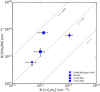 |
Fig. 6 Correlation of the column densities of CH3OH and c-C3H2 towards the four protostars in our sample. The sources are labeled in the legend in the bottom right corner. The dashed lines indicate a CH3OH/c-C3H2 column density ratio of 100, 10, and 1. |
5.1.2 iCOM broad line emission from hot corino
L1551-IRS5 is associated with a hot corino (Bianchi et al. 2020), and shows broad (~3 km s−1) line profiles of CH3OH, CH3CN, CH3CHO, and HCOOCH3 (see the bottom right panel of Fig. 5).
In addition, the LVG solutions on CH3OH and CH3CN show compact source sizes (0.′′18 and 0.′′11, respectively) and kinetic temperatures higher than 50 K, up to 135 K. This is consistent with the chemistry expected for methanol (i.e., a formation uniquely on dust mantles) (e.g., Tielens & Hagen 1982; Rimola et al. 2014), and a thermal desorption due to protostellar heating (e.g., Charnley et al. 1992; Maret et al. 2005). In principle, CH3CN can be formed in two ways, through gas-phase and grain-surface reactions (e.g., Walsh et al. 2014). CH3CHO, and HCOOCH3 are thought to form either on the grain surfaces before evaporating onto the gas phase or in the gas phase using simpler species from the dust mantle (e.g., Garrod & Herbst 2006; Balucani et al. 2015; Vazart et al. 2020; Jørgensen et al. 2020, and references therein).
On the other hand, we did not detect any hot corino activity towards the other three protostars of our sample: L1489-IRS, B5-IRS1, and L1455-IRS1.We report 3σ upper limits on the column densities of iCOMs in Table 7 by assuming Trot = 150 K and a FWHM = 3 km s−1. The column densities are lower than ~1013 cm−3 (CH3OH, HCOOCH3), and ~1011–1012 cm−3 (CH3CN, CH3CHO). Recently, Yang et al. (2021) mapped with ALMA several O-bearing and N-bearing iCOMs at high Eup (up to ~850 K) towards Class 0 and Class I protostars in Perseus, L1455-IRS1 and B5-IRS1 among them. Yang et al. (2021) imaged a hot corino towards these sources, while no extended emission is present. No column density is reported for L1455-IRS1, while for B5-IRS1 they report a NCH_3OH = 5 × 1015 cm−2 measured in the inner 0.′′5. Once diluted in the IRAM-30 m beam, the methanol column density of the hot corino would be ~1013 cm−2. This value is consistent with the upper limits on the iCOMs column densities reported in Table 7. Conversely, the present IRAM-30 m detection of the extended narrow CH3OH emission in B5-IRS1 (and those reported by Öberg et al. 2014) could have been filtered out by the ALMA images by Yang et al. (2021).
Upper limits (3σ) on the column densities of the iCOMs detected in L1551-IRS5 towards L1489-IRS, B5-IRS1, and L1455-IRS1.
5.1.3 H2S, H2 CS, and OCS: Hot corinos and circumbinary disks
The abundance of sulfur in our Solar System is S∕H = 1.8 × 10⁻⁵ (Anders & Grevesse 1989). However, it is well known that sulfur in star forming regions is depleted by at least two orders of magnitude with respectto this value (e.g., Tieftrunk et al. 1994; Wakelam et al. 2004; Laas & Caselli 2019; van ’t Hoff et al. 2020). In addition, the main S-carrier species on dust grains has not been firmly identified yet (Boogert et al. 2015). Historically the most plausible suspect was H2S, which is expected to be formed by surface reactions in the dust mantle, due to high hydrogenation and mobility of H. An alternative solution is OCS (e.g., Wakelam et al. 2004; Codella et al. 2005; Podio et al. 2014; Holdship et al. 2016; Taquet et al. 2020), which is potentially formed on grain surfaces by the addition of oxygen to the CS molecule. However, neither H2S nor OCS have been observed in interstellar ices (Boogert et al. 2015). The possible role of H2CS has also been discussed in light of observations of protostellar shocks, where the dust composition is injected into the gas phase (Codella et al. 2005), but H2CS is now thought to be mainly formed by different neutral-neutral and gas phase reactions of CH and S (Yamamoto 2017). Interestingly, H2S and H2CS have been recently detected and imaged using ALMA towards a number of protoplanetary disks (Phuong et al. 2018; Le Gal et al. 2019; Loomis et al. 2020; Codella et al. 2020). This means that the observation of H2S, H2CS, and OCS towards Class I objects can be used to investigate how the molecular complexity of the early star formation stages changes with time.
Narrow (≤1 km s−1) H2CS emission has been observed towards both B5-IRS1 and L1455-IRS1, suggesting an emission from the molecular gas of the envelope. L1551-IRS5 shows a ~3 km s−1 wide H2CS line centered at the systemic velocity consistent with the envelope origin. On the contrary, H2S and OCS detected towards L1455-IRS5 and L1551-IRS5 are completely different with respect to H2CS, both showing broad (≥5 km s−1) emission. Rotational diagrams of OCS (Eup ≥ 100 K) in both objects (see Figs. B.3 and B.4) suggest that it traces warm gas. This is in agreement with the idea that OCS and H2S are among the expected S-bearing species released from the ice mantles of dust grains in hot corinos. Interestingly, L1455-IRS1 and L1551-IRS5 are binary systems resolved by interferometric images (e.g., Tobin et al. 2018; Takakuwa et al. 2020; Yang et al. 2021) associated with circumbinary disks. More specifically, Takakuwa et al. (2020) showed that OCS traces not only the two protostars, but also and mainly the circumbinary disk around the two L1551-IRS5 objects. The OCS traced by ALMA emits in the same velocity range here observed with the IRAM-30 m. These findings, coupled with the similarity of OCS and H2S spectra in L1551-IRS5 and L1455-IRS1 suggest that H2S is also associated with the circumbinary disks of the sources. To confirm this hypothesis, it is necessary to observe the structures with high-resolution images. The complexity of L1551-IRS5 spectra (produced by emission due to two hot corinos and an envelope) is discussed in detail in Sect. 5.2.
5.2 The L1551-IRS5 system
L1551-IRS5 is a binary system composed of two protostars, called the northern and southern components (e.g., Cruz-Sáenz de Miera et al. 2019; Bianchi et al. 2020, and references therein). L1551-IRS5 is a unique protostar in our sample since it presents both hydrocarbons and hot corino activity with iCOM emission, as discussed in Sects. 4.5.2, 4.4.3, and 5.1.
The systemic velocities of the northern and southern components are +7.5 km s−1 and +4.5 km s−1, respectively (Bianchi et al. 2020). The velocity of the circumbinary envelope is +6.4 km s−1, derived using c-C2H3 and C18O. This measurement is in agreement with the C18O images obtained with ALMA by Takakuwa et al. (2020). In light of the information on the systemic velocity of the L1551-IRS5 system, the IRAM-30 m spectra of the region can be analyzed in detail.
Figure 7 summarizes the L1551-IRS5 spectra as observed using different molecules. Most of the detected species peak at the envelope velocity +6.4 km s−1, for example c-C3H2. CH3OH and other detected iCOMs (CH3CN, CH3CHO, and HCOOCH3) peak at thevelocity associated with the northern protostars, which is redshifted by ~1.5 km s−1 with respect to +7.5 km s−1. This findingis in close agreement with the ALMA images of iCOM emission by Bianchi et al. (2020), who showed thatthe northern protostar is associated with a rotating hot corino, being the NW redshifted emission brighter than the SE blueshifted emission. As shown in Sect. 4.5, the LVG results indicate that CH3OH and CH3CN have Tkin ~ 100 K and θ ~ 0.′′15, tracing the hot corino region around the northern protostar.
Finally, H2S (blue line in Fig. 7) and OCS show profiles that differ from that of the envelope and of the northern hot corino. There are two peaks, the first redshifted with respect to the velocity of the northern component, but the second emission peak occurs at 4.5 km s−1 (i.e., the velocity of the southern components of the L1551-IRS5 binary system). Our H2S and OCS spectra can be interpreted in light of the C18O and OCS ALMA observations at the 10 au spatial scale reported by Takakuwa et al. (2020), who reported the presence of two circumstellar disks associated with the two companions of the binary system, plus emission from the circumbinary disk.
To conclude, the present OCS profile observed with IRAM-30 m is due to the sum of emission close to the protostars and due to emission from the circumbinary disk. Given the similarity of the OCS and H2S profiles we expect that, if observed at 10 au resolution, H2S emission would also be a combination of emission from the hot corinos and the circumbinary disk.
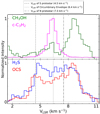 |
Fig. 7 Normalized intensity profiles of four species towards L1551-IRS5. The spectra of CH3OH in green and c-C3H2 in pink in the upper panel are obtained after stacking the detected transitions (see Fig. 5). The spectra of H2S in blue and OCS in red in the lower panel are transitions 22,0–21,1 and 19–18, respectively (see Fig. A.4). The dashed and dash-dotted lines represent the systemic velocities of the southernprotostar (4.5 km s−1) and the northern protostar (7.5 km s−1), respectively (Bianchi et al. 2020), while the dotted line represents the systemic velocity of the circumbinary envelope (6.4 km s−1) measured using the C18O 2–1 line (this work). |
5.3 Chemical evolution along the star formation process
5.3.1 Deuterium fractionation
As we note in Sect. 1, molecular deuteration is very important in order to understand the chemical evolution from prestellar cores to comets. To date, a collection of deuterated species have been detected from the prestellar phase to small bodies of the Solar System (e.g., Caselli & Ceccarelli 2012; Ceccarelli et al. 2014). However, to our best knowledge, there is a limited number of studies on deuteration in Class I protostars.
By studying the prototypical Class I protostar SVS13-A, Bianchi et al. (2017a, 2019a) reported a decrease in the deuteration of methanol, thioformaldehyde, and formaldehyde with respect to what is found towards Class 0 objects. With the results obtained for the four Class I sources in our sample, we can verify what is found in SVS13-A. Table 8 reports the deuteration measurements towards our sample.
For double-deuterated formaldehyde in L1489-IRS, B5-IRS1, L1455-IRS1, and L1551-IRS5, we measured the abundance ratios [D2CO]/[H2CO] = N /N
/N . From the abundance ratios, we derive the deuterium fractionation as D/H
 ![Mathematical equation: $=\sqrt{\mathrm{[D_2CO]/[H_2CO]}}$](/articles/aa/full_html/2022/03/aa41790-21/aa41790-21-eq24.png) (Manigand et al. 2019). We found D/H of 9−13%, ~ 24−55%, ~ 28−53%, and ~ 45−84%, respectively.
(Manigand et al. 2019). We found D/H of 9−13%, ~ 24−55%, ~ 28−53%, and ~ 45−84%, respectively.
Figure 8 compares our results with what has been obtained for SVS13-A and with the deuteration levels measured, using single-dish telescopes, in Class 0 sources and prestellar cores (Bacmann et al. 2003; Parise et al. 2006; Watanabe et al. 2012; Bianchi et al. 2017a; Chacón-Tanarro et al. 2019). We also added interferometric measurements towards Class 0 sources (Persson et al. 2018; Manigand et al. 2020). Figure 8 shows that with an increased number of [D2CO]/[H2CO] measurements towards Class I there is no significant change moving from the prestellar core to the Class I stage.
In the case of L1551-IRS5 we have emission of methanol and single-deuterated methanol, CH2DOH, from different regions that are kinematically distinct in the line spectra (see Fig. 7), such as the envelope and the hot corino. Thus, we estimate the abundance ratios, [CH2DOH]/[CH3OH], for the hot corino and the envelope separately, and we indicate these different measurements in Fig. 8.
The corresponding D/H ratios are derived as D/H = 1/3 [CH2DOH]/[CH3OH] (Manigand et al. 2019) and are 6–23% (B5-IRS1), 1–2% (L1455-IRS1), and ≤1% (L1551-IRS5 envelope). In addition, for the L1551-IRS5 hot corino, [CH2DOH]/[CH3OH] is ~2−10%, which gives a D/H ratio of 0.7–3%. Figure 8 reports, as was done for [D2CO]/[H2CO], the comparison of our measurements with what is presented in literature, from prestellar cores to Class I protostars (e.g., Bianchi et al. 2017b; Jørgensen et al. 2018; Jacobsen et al. 2019; van Gelder et al. 2020; Manigand et al. 2020). Hot corinos are highlighted by dashed areas. Overall, the measurements are consistent ([CH2DOH]/[CH3OH] ~ 0.1 within an order of magnitude) moving along the different evolutionary stages. An exception is provided by the SVS13-A envelope, which shows a lower D/H ratio (~ 10−3). Interestingly, upper limits on the [CH2DOH]/[CH3OH] ratio obtained for comets (Hale-Bopp and 67P/C-G; Crovisier et al. 2004; Drozdovskaya et al. 2021) suggest that the methanol deuteration is not significantly different from the previous stages (from prestellar core to Class I protostar). This could suggest that methanol formed onto dust grains can be inherited from earlier phases (Drozdovskaya et al. 2021). Better statistics, provided by an increase in the measurements for comets, could help to test the inheritance scenario suggested by Fig. 8.
Finally, Fig. 8 also reports the [HDCS]/[H2CS] abundance ratios in L1455-IRS1 and L1551-IRS5. The D/H ratios are derived as D/H = 1/2 [HDCS]/[H2CS] (Manigand et al. 2019) and are 9–14% (L1455-IRS1) and 5–15% (L1551-IRS5). These two measurements together with the limited number of previous measurements so far are reported by Marcelino et al. (2005), Vastel et al. (2018), Drozdovskaya et al. (2018), and Bianchi et al. (2019b). This also suggests that for H2CS the level of deuterium fractionation is constant from the prestellar core to the Class I stage. A comparison between the deuteration of S-bearing molecules with that of complex organics could be instructive for astrochemical models of star forming regions (Taquet et al. 2019). Thioformaldehyde is one of the few S-bearing species imaged in protoplanetary disks (Le Gal et al. 2019; Codella et al. 2020). Marcelino et al. (2005) modeled the Barnard 1 dark cloud using a steady-state gas-phase chemical network in environments with different level of sulfur depletion. According to their results the [HDCS]/[H2CS] ratio is ~0.2, which is consistent with the ratios that we estimated towards L1455-IRS1 and L1551-IRS5.
In general, the early stages of low-mass star formation are characterized by high deuteration (see, e.g., Parise et al. 2004, 2006; Aikawa et al. 2012; Caselli & Ceccarelli 2012; Ceccarelli et al. 2014). In high-density and low-temperature prestellar cores, where CO is highly depleted, the D/H abundance in the gas phase is dramatically enhanced. In addition, the deuteration observed at the protostellar stages, when the dust mantles are injected back to the gas phase, can be used as a fossil to retrace the history of interstellar ices. The deuteration of a molecule can indirectly tell us what the density was (and the temperature) when this species froze out (Aikawa et al. 2012; Taquet et al. 2012, 2014, 2019). More specifically, CH2DOH and D2CO increase their abundance on dust grain surfaces once several mantle layers have been deposited due to freeze-out. As a consequence, the inner protostellar regions, where the ice mantle is evaporated is expected to be less deuterated with respect to the outer envelope region where only the external layer is injected into the gas phase. Figure 8 shows that, with the exception of SVS13-A, the measurements of [CH2DOH]/[CH3OH] for envelopes and hot corinos is ~0.01−0.1. Within one order of magnitude, these numbers are consistent with the ranges provided by Taquet et al. (2014, 2019). Figure 8 shows that the observed [D2CO]/[H2CO] ratios are spread over two orders of magnitude (~0.01–1). The theoretical models by Taquet et al. (2014) predict abundance ratios from 10−4 to 10−1, a range that is too large for a proper comparison with observations. The observations are also not fit by the gas-grain reaction network applied to a one-dimensional radiative hydrodynamic model by Aikawa et al. (2012), predicting a deuteration lower by about three orders of magnitude.
In conclusion, when the large sample of Class I sources is considered, the CH3OH and (double) H2CO deuteration observed from the prestellar core to Class I protostellar phases is roughly constant and similar to that measured in comets. This suggests that the D/H value set at the prestellar stage is inherited by the later phases of the star forming process. However, recent Rosetta measurements of D/H in the organic refractory component of cometary dust particles in 67P/C-G (Paquette et al. 2021) showed that D/H is 1.6 ± 0.5 × 10⁻³, an order of magnitude lower than deuteration in the organics measured in gas phase towards prestellar cores, protostars, and the cometary coma in Fig. 8. This puts into question the inheritance of D/H from the protostellar phase. Therefore, more observations of D/H in the organic refractory molecules towards comets are needed to test the chemical inheritance hypothesis.
Abundance ratios of the deuterated molecule to the non-deuterated molecule and inferred D/H ratios in the observed Class I sources.
 |
Fig. 8 Abundance ratios [XD]/[XH] measured for organic species in sources at different evolutionary stages: prestellar cores (D2CO (Bacmann et al. 2003; Chacón-Tanarro et al. 2019), CH2DOH (Bizzocchi et al. 2014; Chacón-Tanarro et al. 2019; Ambrose et al. 2021), and HDCS (Marcelino et al. 2005; Vastel et al. 2018)); Class 0 protostars (D2CO (Parise et al. 2006; Watanabe et al. 2012; Persson et al. 2018; Manigand et al. 2020), CH2DOH (Parise et al. 2006; Bianchi et al. 2017b; Jørgensen et al. 2018; Jacobsen et al. 2019; van Gelder et al. 2020; Manigand et al. 2020), and HDCS (Drozdovskaya et al. 2018); Class I protostars (SVS13-A; D2CO, CH2DOH (Bianchi et al. 2017a), and HDCS (Bianchi et al. 2019a)); comets (Hale-Bopp; CH2DOH (Crovisier et al. 2004) and 67P/C-G; CH2DOH (Drozdovskaya et al. 2021)). The [XD]/[XH] values inferred for L1489-IRS, B5-IRS1, L1455-IRS1, and L1551-IRS5 are in magenta (from this work). The dashed bars represent values inferred for the hot corinos (r ≤ 100 au, T ≥ 100 K), while the filled bars indicate the measurements derived for extended envelope. |
5.3.2 Chemical richness
As reported in Sect. 1, Class I sources are expected to play a key role in understanding if and how the chemical composition is transmitted from the earliest stages of a Sun-like forming star, from the parental cloud (prestellar cores) to the small-bodies in the Solar System (such as comets). To address this ambitious goal, we compare the abundance ratios of iCOMs, as well as the abundance ratios of simpler molecules ([CH3OH]/[H2CO] and [H2CS]/[H2CO]) obtained forthe Class I protostars in our sample with the values obtained for prestellar cores, hot corinos, and envelopes around Class 0 protostars, protoplanetary disks, and comets.
In the first panel of Fig. 9 we show the ratios of the iCOM CH3CN (as a lower limit), CH3CHO, and HCOOCH3 with respect to CH3OH for the L1551-IRS5 hot corino (magenta circle). To estimate these abundance ratios we use the column densities of CH3CN and CH3OH obtained from the LVG analysis, which takes into account the source size. For CH3CHO and HCOOCH3, we assume a source size of 0.′′18 (i.e., the source size of CH3OH) and correct for the beam filling factor. The [CH3CN]/[CH3OH], [CH3CHO]/[CH3OH], and [HCOOCH3]/[CH3OH] abundance ratios are ≥0.02, 0.04 ± 0.015, and 0.07 ± 0.01, respectively. Our measurements are compared with those derived towards chemically rich hot corinos in the literature. We consider only interferometric measurements in order to minimize the effects due to beam dilution. The Class 0 sources are IRAS 16293-2422A and B (PILS ALMA survey; Jørgensen et al. 2016, 2018; Calcutt et al. 2018; Manigand et al. 2020), HH212 (Lee et al. 2019a), the CALYPSO IRAM PdBI sources (Belloche et al. 2020), and the PEACHES ALMA sources (Yang et al. 2021). For the Class I sources we report Ser-17 (Bergner et al. 2019), L1551-IRS5 (FAUST ALMA Bianchi et al. 2020), and the PEACHES ALMA sources (Yang et al. 2021). In addition, we plot the values obtained for the V883 Ori protoplanetary disk (Lee et al. 2019b), and what is measured towards several comets: Hale-Bopp, Hyakutake, LINEAR, Lovejoy, 73P/SW3/B, 73P/SW3/C, 67P summer hemisphere, and 67P winter hemisphere (Le Roy et al. 2015).
Figure 9 shows that the abundance ratios between CH3CN, CH3CHO, and HCOOCH3 with respect to CH3OH in L1551-IRS5 are in agreement (within an order of magnitude) with those measured in Class 0 and other Class I hot corinos. In addition, Fig. 9 shows that similar values are derived for the V883 Ori protoplanetary disk and for comets. The only exception is given by the [CH3CN]/[CH3OH] ratio in V883 Ori, which is roughly one order of magnitude lower than what is shown by the rest of the sample. To conclude, the overall suggestion provided by Fig. 9 is that the molecular complexity characterizing an evolutionary stage of low-mass star formation could be inherited from the previous phase. Clearly, in order to verify this picture, the statistics need to be improved, in particular with regard to the more evolved Class II disks.
In addition to iCOMs, Fig. 9 also shows the [CH3OH]/[H2CO] and [H2CS]/[H2CO] abundance ratios derived for our Class I sources by considering the emission from both the hot corinos and the envelopes. These abundance ratios are compared with those obtained for (i) the prestellar cores L1544 (Chacón-Tanarro et al. 2019) and Barnard 1 (Marcelino et al. 2005); (ii) the Class 0 IRAS 16293-2422A and B (Jørgensen et al. 2018; Persson et al. 2018; Manigand et al. 2020; Drozdovskaya et al. 2018), NGC 1333-IRAS 4A and IRAS 2A (Taquet et al. 2015); (iii) the Class I SVS13-A (Bianchi et al. 2017a, 2019b); (iv) the protoplanetary disks IRAS 04302+2247, HL Tau, TW Hya, and HD 100546 (Walsh et al. 2016; Carney et al. 2019; Codella et al. 2020; Podio et al. 2020; Garufi et al. 2021; Booth et al. 2021); and (v) the comets Lovejoy, Hale-Bopp, and 67P/C-G (Biver et al. 2015; Rubin et al. 2019). The range of the [CH3OH]/[H2CO] abundance ratios towards L1489-IRS, B5-IRS1, L1455-IRS1, and L1551-IRS5 are 0.4–0.9, 0.2–0.7, 1.0–2.2, and 0.3–0.9, respectively. These ratios (derived towards the extended envelope) are consistent with the values measured in protoplanetary disks and comets and in prestellar cores (Fig. 9, bottom left) with the exception of the envelope of SVS13-A.
On the other hand, the abundance ratios for the four hot corinos derived from interferometric observations of Class 0 protostars (dashed box) is up to 2 orders of magnitude higher. From our survey we derive for the L1551-IRS5 hot corino a lower limit on the [CH3OH]/[H2CO] ratio that is in agreement with the measures derived for Class 0 hot corinos. Thus, [CH3OH]/[H2CO] in the L1551-IRS5 envelope (0.3–0.9) is lower than that in the L1551-IRS5 hot corino (≥30). This effect plausibly reflects the methanol release from icy dust into the gas phase due to thermal evaporation, richer in methanol with respect to the envelope and/or prestellar objects where CH3OH is produced due to non-thermal processes.
Finally, Fig. 9 (bottom right) shows the H2CS-to-H2CO ratio. The reason for measuring this ratio is that if both species are formed in the gas-phase by reactions of atomic O or S with the methyl group CH3, as in the molecular layer of disks (e.g., Fedele & Favre 2020), then their abundance ratio can be used to estimate the elemental S/O abundance ratio. Figure 9 shows that the prestellar core Barnard 1 and the envelopes around Class I objects are associated with a quite similar [H2CS]/[H2CO] ratio, between a few 10−2 and ~1. The ratios for protoplanetary disks and comets also fall in the same range. Conversely, the [H2CS]/[H2CO] as measured in the inner 60 au towards the Class 0 IRAS 16293B is definitely lower (see dashed box; ~10−3, Persson et al. 2018; Drozdovskaya et al. 2018). Only further measurements on Solar System scales will determine whether this difference reflects a real chemical difference with respect to what is measured in the more extended envelope.
 |
Fig. 9 Abundance ratios of organic molecules towards the four protostars. Upper panel: abundance ratios of iCOMs with respect to methanol measured at different evolutionary stages. The three panels (from left to right) refer to CH3CN, CH3CHO, and HCOOCH3, and each is divided into four parts; the gray dashed lines separate the Class 0 sources, Class I sources, protoplanetary disks (PPD), and comets. The abundance ratios estimated for L1551-IRS5 in this work are indicated by a magenta circle. The abundance ratios for the literature sources (see text for references) are labeled in the legend in the bottom right corner. Bottom panels: abundance ratios of [CH3OH]/[H2CO] (left) and [H2CS]/[H2CO] (right) for our Class I sources (magenta bars) compared with the values of prestellar cores, Class 0 sources, PPDs, and comets from the literature, as labeled. The dashed bar in the left panel indicates hot corino measurements, while the dashed bar in the right panel indicates the measurement obtained in the inner 60 au towards the IRAS 16293B protostar. The references of the measurements from the literature are reported in Sect. 5.3.2. |
6 Summary
We have presented a chemical survey of four Class I protostars (L1489-IRS, B5-IRS1, L1455-IRS1, and L1551-IRS5) using IRAM-30 m single-dish observations at 1.3 mm. The main conclusions are summarized as follows.
We detected 157 lines due to 27 species from simple diatomic and triatomic molecules to iCOMs: C-chains (c-C3H, c-C3H2, and CH3CCH), iCOMs (CH3OH, CH3CN, CH3CHO, and HCOOCH3), N-bearing species (13CN, C15N, and HNCO), S-bearing molecules (SO, 34SO, SO2, 13CS, OCS, O13CS, CCS, H2S, H2CS, and H2C33S), SiO, and deuterated molecules (DCO+, N2D+, CCD, DCN, HDCS, D2CO, and CH2DOH). More specifically we detected 17 transitions due to 10 species in L1489-IRS, 29 transitions due to 15 species in B5-IRS1, and 36 transitions due to 21 species in L1455-IRS1. L1551-IRS5 is associated with the highest number of molecules with 75 transitions from 27 species.
We used the standard rotational diagram approach in order to determine the rotational temperatures and to derive the column densities. When applicable, we corrected the obtained column densities from the opacity derived using the emission of rarer isotopologues. The rotational temperature for diatomic and triatomic species in L1489-IRS, B5-IRS1, and L1455-IRS1 is low (≤20 K) suggesting an origin in the envelopes of these sources. Conversely, L1551-IRS5 shows iCOM emission that traces the inner protostellar region with Trot, up to ~150 K. The beam-averaged column densities are between 1011 cm−2 and 1013 cm−2 for all the species but SO and CH3OH, for which we find Ntot of a few 1014 cm−2.
We observed different line profiles: (i) narrow Gaussians (~1 km s−1) centered at systemic velocities, (ii) broader lines (3–4 km s−1) also at systemic velocities, and (iii) line wings extending up to ~30 km s−1 with respect to systemic velocity. The last have been observed in CO, SO, and H2CO and in signatures of the molecular protostellar outflows. Narrow profiles are expected to trace extended emission, plausiblythe molecular envelope. The LVG analysis of the narrow c-C2H3 line emission indicates temperatures in the 5–25 K range, densities higher than 103 cm−3, and sizesbetween 2′′ and 10′′. On the other hand, all iCOMs show broad emission in L1551-IRS5: the LVG analysis of CH3OH and CH3CN emission points to kinetic temperatures higher than 50 and up to 135 K, densities higher than 3 × 105 cm−3, and a size of 0.′′11–0.′′18 (~16–25 au), confirming the presence of a hot corino.
The CH3OH 42,3–31,2E line (Eup = 45 K) shows narrow (~1 km s−1) line emission, and has the same profile of the envelope tracer c-C3H2. The emission is expected to trace the external layers of the envelope or the outflow cavities hit by UV radiation.
We suggest that H2S and OCS trace hot corinos as well as circumstellar disks in the previously confirmed binary systems, L1455-IRS1 and L1551-IRS5. To confirm this hypothesis, it is needed to observe these S-bearing species with high-resolution images in several binaries.
We derived the elemental deuterium fractionation through the following abundance ratios: D2CO/H2CO, HDCS/H2CS, and CH2DOH/CH3OH. The derived D/H ratios in the envelope are 10–70% (D2CO/H2CO), 5–15% (HDCS/H2CS), and 1–23% (CH2DOH/CH3OH). For the L1551-IRS5 hot corino we derive for deuterated methanol D/H ~ 0.7–3%. These measurements are similar to what is reported for earlier star forming stages, supporting the inheritance scenario from prestellar cores to Class I sources.
We computed the column density ratios between three iCOMs (CH3CN, CH3CHO, and HCOOCH3) and CH3OH in the L1551-IRS5 hot corino, which are between 0.04 and 0.07. The comparison of these values with what is measured in Class 0, other Class I sources, protoplanetary disks, and comets suggests that the iCOM abundance ratios are constant during the formation process of a Sun-like star. This supports the hypothesis that the chemical complexity at the planet forming stage is inherited from the earlier star formation stages.
The [CH3OH]/[H2CO] abundance ratio in L1551-IRS5 is higher in the hot corino than in the envelope, in agreement with an increase in the methanol abundance due to thermal evaporation of the dust mantles in the hot corino.
The results obtained with our IRAM-30 m 1.3 mm observations provide crucial information on the chemical richness of Class I sources and on the chemical evolutionary path along the low-mass star forming process. More observations of the different evolutionary stages are needed to better understand the evolution of the abundance ratios. In particular, higher spatial resolution observations and images are needed to disentangle the complexity of each component around protostars. In this context, the NOEMA large program Seeds Of Life In Space (SOLIS, Ceccarelli et al. 2017), the ALMA large program Fifty AU Study of the chemistry in the disk/envelope system of solar-like protostars7 (FAUST, Bianchi et al. 2020), as well as the ALMA Perseus ALMA Chemistry Survey (PEACHES, Yang et al. 2021) are expected to provide much more information on the molecular complexity for larger samples of solar-like protostars.
Acknowledgements
We thank the IRAM-30 m staff for its valuable help during the observations. This project has received funding from the European Union’s Horizon 2020 research and innovation programme under the Marie Skłodowska-Curie grant agreement No 811312 for the project “Astro-Chemical Origins” (ACO) and from the European Research Council (ERC) under the European Union’s Horizon 2020 research and innovation programme, for the Project “The Dawn of Organic Chemistry” (DOC), grant agreement No 741002. We also thank Paola Caselli and Luca Dore for fruitful discussion regarding the hyperfine components.
Appendix A Detected lines and observed spectra
In this section we present the detected molecules with the spec- tra for each protostar in Figures A.1 – A.4. In Figures A.5 and A.6 we present the observed spectra of CO and its isotopologues with their isotopic ratios. We also report, for each source and for each detected line, the spectral line parameters as well as the results of the spectral fit: frequency (MHz), telescope HPBW (′′), upper level energies Eup (K), Sμ2 product (D2), rms (mK), peak temperature (mK), spectral resolution δv (km s−1), peak velocity (kms−1), FWHM (km s−1), velocity integrated line intensity Iint (mK km s−1) from Tables A.1 to A.4.
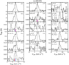 |
Fig. A.1 Spectra observed towards L1489-IRS (see Table A.1 in TMB scale). Species, transition, and upper level energy are reported in each panel. The vertical dashed line stands for the source systemic velocity measured using the C18O(2–1) line (+7.3 km s−1). In the CCD(3–2) spectrum the velocity scale is centered on the brightest (3 D2) hyperfine component (vertical blue line) at 216372.8 MHz; the vertical red lines indicate the offset in velocity of the fainter components (1.9 D2 at 216373.3 MHz; 1.4 D2 at 216373.2 MHz. This spectrum is smoothed to 0.40 MHz. In the C15N(2–1) spectrum (lower panel) the velocity scale is centered on the brightest (6 D2) hyperfine component (vertical blue line) at 219934.8 MHz; the vertical red line indicates the offset in velocity of the fainter components (4 D2 at 219934.0 MHz). In the DCN(3–2) spectrum the velocity scale is centered on the brightest (35 D2) hyperfine component (vertical blue line) at 217238.3 MHz; the vertical red lines indicate the offset in velocity of the fainter components (20 D2 at 217238.6 MHz; 16 D2 at 217238.3 MHz). |
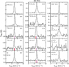 |
Fig. A.2 Spectra observed towards B5-IRS1 (see Table A.2 in TMB scale). Species, transition, and upper level energy are reported in each panel. The vertical dashed line stands for the source systemic velocity measured using the C18O(2–1) line (+10.2 km s−1). In the 13CN(2–1) spectrum the velocity scale is centered on the brightest (8 D2) hyperfine component (vertical blue line) at 217467.1 MHz; the vertical red line indicates the offset in velocity of the fainter component (5 D2 at 217467.1 MHz). In the 13CS(5–4) spectrum the velocity scale is centered on the brightest (38 D2) hyperfine component (vertical blue line) at 231220.7 MHz; the vertical red lines indicate the offset in velocity of the fainter components (21 D2 at 231220.7 MHz; 17 D2 at 231220.6 MHz; 1 D2 at 231220.5 MHz). In the CCD(3–2) spectrum (middle panel, middle column) the velocity scale is centered on the brightest (3 D2) hyperfine component (vertical blue line) at 216372.8 MHz; the vertical red lines indicate the offset in velocity of the fainter components (1.9 D2 at 216373.3 MHz; 1.4 D2 at 216373.2 MHz). Lower panel: In the CCD(3–2) spectrum the velocity scale is centered on the brightest (2 D2) hyperfine component (vertical blue line) at 216428.3 MHz; the vertical red line indicate the offset in velocity of the fainter components (0.7 D2 at 216428.8 MHz). In the DCN(3–2) spectrum the velocity scale is centered on the brightest (35 D2) hyperfine component (vertical blue line) at 217238.3 MHz; the vertical red lines indicates the offset in velocity of the fainter components (20 D2 at 217238.6 MHz; 16 D2 at 217238.3 MHz). |
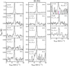 |
Fig. A.2 Continued: Spectra observed towards B5-IRS1 (see Table A.2 in TMB scale). In theo- c-C3H2 spectrum the velocity scale is centered on the brightest (63 D2) hyperfine component (vertical blue line) at 218449.4 MHz; the vertical red line indicates the offset in velocity of the fainter components (21 D2 at 216448.8 MHz). The CH2DOH spectrum is smoothed to 0.40 MHz. |
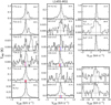 |
Fig. A.3 Spectra observed towards L1455-IRS1 (see Table A.3 in TMB scale). Species, transition, and upper level energy are reported in each panel. The vertical dashed line stands for the source systemic velocity measured using the C18O(2–1) line (+4.7 km s−1). In the 13CN(2–1) spectrum the velocity scale is centered on the brightest (8 D2) hyperfine component (vertical blue line) at 217467.1 MHz; the vertical red line indicates the offset in velocity of the fainter component (5 D2 at 217467.1 MHz). In the 13CS(5–4) spectrum the velocity scale is centered on the brightest (38 D2) hyperfine component (vertical blue line) at 231220.7 MHz; the vertical red lines indicate the offset in velocity of the fainter components (21 D2 at 231220.7 MHz; 17 D2 231220.6 MHz; 1 D2 at 231220.5 MHz). In the CCD(3–2) spectrum (fourth row) the velocity scale is centered on the brightest (2 D2) hyperfine component (vertical blue line) at 216428.3 MHz; the vertical red line indicates the offset in velocity of the fainter components (0.7 D2 at 216428.8 MHz). Lower panel: In the CCD(3–2) spectrum the velocity scale is centered on the brightest (3 D2) hyperfine component (vertical blue line) at 216372.8 MHz; the vertical red lines indicate the offset in velocity of the fainter components (1.9 D2 at 216373.3 MHz; 1.4 D2 at 216373.2 MHz). In the DCN(3–2) spectrum the velocity scale is centered on the brightest (35 D2) hyperfin component (vertical blue line) at 217238.3 MHz; the vertical red lines indicate the offset in velocity of the fainter components (20 D2 at 217238.6 MHz; 16 D2 at 217238.3 MHz). |
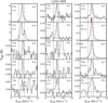 |
Fig. A.4 Spectra observed towards L1551-IRS5 (see Table A.4 in TMB scale). Species, transition, and upper level energy are reported in each panel. The vertical dotted line stands for the source systemic velocity as measured using the C18O(2–1) line (+6.4 km s−1). The vertical dashed line and the vertical dash-dotted line stand for the systemic velocities of the binary system associated with the southern source (+4.5 km s−1) and northern source (+7.5 km s−1), respectively. In the 13CS(5–4) spectrum the velocity scale is centered on the brightest (38 D2) hyperfine component (vertical blue line) at 231220.7 MHz; the vertical red lines indicate the offset in velocity of the fainter components (21 D2 at 231220.7 MHz; 17 D2 at 231220.6 MHz; 1 D2 at 231220.5 MHz). In the C15N(2–1) spectrum (lower panel) the velocity scale is centered on the brightest (6 D2) hyperfine component (vertical blue line) at 219934.8 MHz; the vertical red lines indicate the offset in velocity of the fainter components (4 D2 at 219934.0 MHz). |
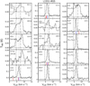 |
Fig. A.4 Continued: Spectra observed towards L1551-IRS5 (see Table A.4 in TMB scale). Lower left panel of the first column: In the CCD(3–2) spectrum the velocity scale is centered on the brightest (2 D2) hyperfine component (vertical blue line) at 216428.3 MHz; the vertical red lines indicate the offset in velocity of the fainter components (0.3 D2 at 216430.3 MHz; 0.7 D2 at 216428.8 MHz). Upper middle panel: In the CCD(3–2) spectrum the velocity scale is centered on the brightest (3 D2) hyperfine component (vertical blue line) at 216372.8 MHz; the vertical red lines indicate the offset in velocity of the fainter components (1.9 D2 at 216373.3 MHz; 1.4 D2 at 216373.2 MHz). In the DCN(3–2) spectrum the velocity scale is centered on the brightest (35 D2) hyperfine component (vertical blue line) at 217238.3 MHz; the vertical red lines indicate the offset in velocity of the fainter components (20 D2 at 217238.6 MHz; 16 D2 at 217238.3 MHz). In the N2D+ spectrum the velocity scale is centered on the brightest (312 D2) hyperfine component (vertical blue line) at 231319.9 MHz; the vertical red line indicates the offset in velocity of the brightest transition of 40 fainter components (5 D2 at 231324.5 MHz). |
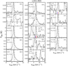 |
Fig. A.4 Continued: Observed spectra observed towards L1551-IRS5 (see Table A.4 in TMB scale). In thec-C3H(41,3–31,2) spectrum the velocity scale is centered on the c-C3H2 emission (vertical blue line) at 216492.6 MHz; the vertical red line indicates possible contamination due to D2CO(81,7–81,8) at 216492.4 MHz. In the H2C33S(71,7–61,6) spectrum the velocity scale is centered on the brightest (67 D2) hyperfine component (vertical blue line) at 234678.8 MHz; the vertical red lines indicate the offset in velocity of the fainter components (58 D2 at 234678.7 MHz; 2 D2 234676.9 MHz). |
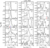 |
Fig. A.4 Continued: Observed spectra of the molecules, towards L1551-IRS5, listed in Table A.4 (in TMB scale). In theo-c-C3H2 spectrum the velocity scale is centered on the brightest (63 D2) hyperfine component (vertical blue line) at 218449.4 MHz; the vertical red lines indicate the offset in velocity of the fainter components (21 D2 at 216448.8 MHz). In the CH3OH spectrum the velocity scale is centered on the CH3OH emission at 231281.1 MHz; the vertical red line indicates possible contamination due to CH3CHO at 231278.5 MHz. |
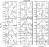 |
Fig. A.4 Continued: Observed spectra of the molecules, towards L1551-IRS5, listed in Table A.4 (in TMB scale). In theCH3CCH spectrum the velocity scale is centered on the CH3CCH emission at 222128.8 MHz; the vertical red line indicates possible contamination due to HCOOCH3 at 222128.2 MHz. In the three HCOOCH3 spectra the spectra are centered on the brightest component (vertical blue line) and the vertical red lines indicate the offset in velocity and strength of the fainter components reported in Table A.4. |
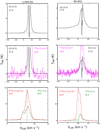 |
Fig. A.5 Observed spectra of CO isotopologues (in TMB scale) towards L1489-IRS (left column) and B5-IRS1 (right column). Species, transition, and upper level energy are reported in each panel. For the panels in the left column the vertical dashed lines stand for the source systemic velocity as measured using C18O (2-1) emission (+7.3 km s−1). For the panels in the right column the vertical dashed lines stand for the source systemic velocity measured using C18O (2-1) emission (+10.2 km s−1). Top panels: CO (2-1) transition. Middle panels: Zoom-in on the CO (2-1) line wings (in black) and the 13CO (2-1) line wings (in magenta), scaled by a factor of 77 in the TMB range from -2 K to 2.5 K. Bottom panels: 13CO (in green) and C18O (in red) scaled by a factor of 7.27 assuming isotopic ratios of 12C/13C = 77 and 16O/18O = 560 (Milam et al. 2005). |
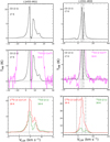 |
Fig. A.6 Observed spectra of CO isotopologues (in TMB scale) towards L1455-IRS1 (left column) and L1551-IRS5 (right column). Species, transition, and upper level energy are reported in each panel. For the panels in the left column the vertical dashed lines stand for the source systemic velocity as measured using C18O (2-1) emission (+4.7 km s−1). For the panels in the right column the vertical dotted line stands for the source systemic velocity measured using the C18O(2–1) line (+6.4 km s−1). The vertical dashed line and the vertical dash-dotted line stand for the systemic velocities of the binary system associated with the southern source (+4.5 km s−1) and northern source (+7.5 km s−1) respectively.Top panels: CO (2-1) transition. Middle panels: Zoom-in on the CO (2-1) line wings (in black) and the 13CO (2-1) line wings (in magenta), scaled by a factor of 77 in the TMB range from -2 K to 2.5 K. Bottom panels: 13CO (in green) and C18O (in red) scaled by a factor of 7.27 assuming isotopic ratios of 12C/13C = 77 and 16O/18O = 560 (Milam et al. 2005). |
List of transitions and observed line properties detected towards L1489-IRS
List of transitions and observed line properties detected towards B5-IRS1
List of transitions and observed line properties detected towards L1455-IRS1
List of transitions and observed line properties detected towards L1551-IRS5
Appendix B Rotational diagrams and derived column densities
We report in Figures B.1–B.4 (one per source) the rotational diagrams obtained from the whole emitting velocity range, as described in Sect. 4. When applicable, ortho and para species and A- and E-types have been analyzed separately. Tables B.1–B.4 report the beam-averaged column densities derived from rotational diagrams. In addition, they include column densities towards envelopes, outflows, and hot corinos. Source-averaged column densities can be derived by applying the filling factors reported in Table 6 for c-C3H2 as an envelope tracer, and for CH3OH and CH3CN as hot corino tracers. For single lines, column densities are derived using the temperature mentioned in Sect. 4.4.
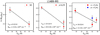 |
Fig. B.1 Rotational diagrams of SO, H2CO, and c-C3H2 in L1489-IRS. The parameters Nup, gup, and Eup are respectively the column density, the degeneracy, and the energy (with respect to the ground state of each symmetry) of the upper level. The error bars include the errors on the flux, as stated in Table A.1, and the uncertainty of the calibration of 20%. |
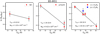 |
Fig. B.2 Rotational diagrams of SO, H2CO, and c-C3H2 in B5-IRS1. The parameters Nup, gup, and Eup are respectively the column density, the degeneracy, and the energy (with respect to the ground state of each symmetry) of the upper level. The error bars include the errors on the flux, as stated in Table A.2, and the uncertainty of the calibration of 20%. |
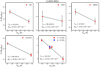 |
Fig. B.3 Rotational diagrams of SO, OCS, HDCS, H2CO, and c-C3H2 in L1455-IRS1. The parameters Nup, gup, and Eup are respectively the column density, the degeneracy, and the energy (with respect to the ground state of each symmetry) of the upper level. The error bars include the errors on the flux, as stated in Table A.3, and the uncertainty of the calibration of 20%. |
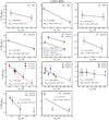 |
Fig. B.4 Rotational diagrams of SO, SO2, OCS, H2CO, D2CO, H2CCO, c-C3H2, CH3OH, CH3CN, CH3CCH, and CH3CHO. The parameters Nup, gup, and Eup are respectively the column density, the degeneracy, and the energy (with respect to the ground state of each symmetry) of the upper level. The derived values of the rotational temperature and the column density are reported in each panel for each species. For D2CO the blue and red circles indicate ortho and para transitions, respectively. For CH3OH the blue and red circles indicate E and A transitions, respectively. Red stars in the c-C3H2 (83,6 – 82,7) and CH3OH (102,9 – 93,6) indicate transitions not used in the fit, due to contamination by other molecules. The blue arrow in the CH3CN panel indicates 124 – 114 transition, which was not used in the fit as upper limit. The error bars include the errors on the flux, as stated in Table A.4, and the uncertainty of the calibration of 20%. |
L1489-IRS: Temperatures and beam-averaged col- umn densities derived for the envelope (see text).
B5-IRS1: Temperatures and beam-averaged column densities for different physical components (envelope, outflow; see text).
L1455-IRS1: Temperatures and beam-averaged column densities for different physical components (envelope, out- flow; see text).
L1551-IRS5: Temperatures and beam-averaged column densities for different physical components (envelope, out- flow, and hot corino; see text).
References
- Adams, F. C., Lada, C. J., & Shu, F. H. 1987, ApJ, 312, 788 [NASA ADS] [CrossRef] [Google Scholar]
- Aikawa, Y., Wakelam, V., Hersant, F., Garrod, R. T., & Herbst, E. 2012, ApJ, 760, 40 [NASA ADS] [CrossRef] [Google Scholar]
- Ambrose, H. E., Shirley, Y. L., & Scibelli, S. 2021, MNRAS, 501, 347 [Google Scholar]
- Anders, E., & Grevesse, N. 1989, Geochim. Cosmochim. Acta, 53, 197 [Google Scholar]
- Andre, P., Ward-Thompson, D., & Barsony, M. 2000, in Protostars and Planets IV, eds. V. Mannings, A. P. Boss, & S. S. Russell (Tucson: University of Arizona Press), 59 [Google Scholar]
- Bacmann, A., Lefloch, B., Ceccarelli, C., et al. 2003, ApJ, 585, L55 [NASA ADS] [CrossRef] [Google Scholar]
- Bally, J., Devine, D., & Alten, V. 1996, ApJ, 473, 921 [NASA ADS] [CrossRef] [Google Scholar]
- Balucani, N., Ceccarelli, C., & Taquet, V. 2015, MNRAS, 449, L16 [Google Scholar]
- Beichman, C. A., Jennings, R. E., Emerson, J. P., et al. 1984, ApJ, 278, L45 [NASA ADS] [CrossRef] [Google Scholar]
- Belloche, A., Maury, A. J., Maret, S., et al. 2020, A&A, 635, A198 [NASA ADS] [CrossRef] [EDP Sciences] [Google Scholar]
- Bergner, J. B., Öberg, K. I., Garrod, R. T., & Graninger, D. M. 2017, ApJ, 841, 120 [Google Scholar]
- Bergner, J. B., Guzmán, V. G., Öberg, K. I., Loomis, R. A., & Pegues, J. 2018, ApJ, 857, 69 [Google Scholar]
- Bergner, J. B., Martín-Doménech, R., Öberg, K. I., et al. 2019, ACS Earth Space Chem., 3, 1564 [NASA ADS] [CrossRef] [Google Scholar]
- Bianchi, E., Codella, C., Ceccarelli, C., et al. 2017a, MNRAS, 467, 3011 [NASA ADS] [CrossRef] [Google Scholar]
- Bianchi, E., Codella, C., Ceccarelli, C., et al. 2017b, A&A, 606, L7 [NASA ADS] [CrossRef] [EDP Sciences] [Google Scholar]
- Bianchi, E., Ceccarelli, C., Codella, C., et al. 2019a, ACS Earth Space Chem., 3, 2659 [NASA ADS] [CrossRef] [Google Scholar]
- Bianchi, E., Codella, C., Ceccarelli, C., et al. 2019b, MNRAS, 483, 1850 [Google Scholar]
- Bianchi, E., Chandler, C. J., Ceccarelli, C., et al. 2020, MNRAS, 498, L87 [NASA ADS] [CrossRef] [Google Scholar]
- Bieging, J. H., & Cohen, M. 1985, ApJ, 289, L5 [Google Scholar]
- Biver, N., Bockelée-Morvan, D., Moreno, R., et al. 2015, Sci. Adv., 1, 11500863 [CrossRef] [Google Scholar]
- Bizzocchi, L., Caselli, P., Spezzano, S., & Leonardo, E. 2014, A&A, 569, A27 [NASA ADS] [CrossRef] [EDP Sciences] [Google Scholar]
- Boogert, A. C. A., Gerakines, P. A., & Whittet, D. C. B. 2015, ARA&A, 53, 541 [Google Scholar]
- Booth, A. S., Walsh, C., Terwisscha van Scheltinga, J., et al. 2021, Nat. Astron., 5, 684 [NASA ADS] [CrossRef] [Google Scholar]
- Bottinelli, S., Ceccarelli, C., Williams, J. P., & Lefloch, B. 2007, A&A, 463, 601 [NASA ADS] [CrossRef] [EDP Sciences] [Google Scholar]
- Bouvier, M., López-Sepulcre, A., Ceccarelli, C., et al. 2020, A&A, 636, A19 [NASA ADS] [CrossRef] [EDP Sciences] [Google Scholar]
- Calcutt, H., Jørgensen, J. K., Müller, H. S. P., et al. 2018, A&A, 616, A90 [NASA ADS] [CrossRef] [EDP Sciences] [Google Scholar]
- Carney, M. T., Hogerheijde, M. R., Guzmán, V. V., et al. 2019, A&A, 623, A124 [NASA ADS] [CrossRef] [EDP Sciences] [Google Scholar]
- Caselli, P., & Ceccarelli, C. 2012, A&ARv, 20, 56 [Google Scholar]
- Ceccarelli, C., Maret, S., Tielens, A. G. G. M., Castets, A., & Caux, E. 2003, A&A, 410, 587 [NASA ADS] [CrossRef] [EDP Sciences] [Google Scholar]
- Ceccarelli, C., Caselli, P., Herbst, E., Tielens, A. G. G. M., & Caux, E. 2007, in Protostars and Planets V, eds. B. Reipurth, D. Jewitt, & K. Keil (Tucson: University of Arizona Press), 47 [Google Scholar]
- Ceccarelli, C., Caselli, P., Bockelée-Morvan, D., et al. 2014, in Protostars and Planets VI, eds. H. Beuther, R. S. Klessen, C. P. Dullemond, & T. Henning (Tucson: University of Arizona Press), 859 [Google Scholar]
- Ceccarelli, C., Caselli, P., Fontani, F., et al. 2017, ApJ, 850, 176 [NASA ADS] [CrossRef] [Google Scholar]
- Chacón-Tanarro, A., Caselli, P., Bizzocchi, L., et al. 2019, A&A, 622, A141 [Google Scholar]
- Chandra, S., & Kegel, W. H. 2000, A&AS, 142, 113 [NASA ADS] [CrossRef] [EDP Sciences] [Google Scholar]
- Charnley, S. B., Tielens, A. G. G. M., & Millar, T. J. 1992, ApJ, 399, L71 [Google Scholar]
- Chen, H., Myers, P. C., Ladd, E. F., & Wood, D. O. S. 1995, ApJ, 445, 377 [NASA ADS] [CrossRef] [Google Scholar]
- Chen, X., Ellingsen, S. P., Ren, Z.-Y., et al. 2019, ApJ, 877, 90 [NASA ADS] [CrossRef] [Google Scholar]
- Chou, H.-G., Yen, H.-W., Koch, P. M., & Guilloteau, S. 2016, ApJ, 823, 151 [NASA ADS] [CrossRef] [Google Scholar]
- Codella, C., Bachiller, R., Benedettini, M., et al. 2005, MNRAS, 361, 244 [Google Scholar]
- Codella, C., Ceccarelli, C., Lefloch, B., et al. 2012, ApJ, 759, L45 [NASA ADS] [CrossRef] [Google Scholar]
- Codella, C., Ceccarelli, C., Cabrit, S., et al. 2016, A&A, 586, L3 [NASA ADS] [CrossRef] [EDP Sciences] [Google Scholar]
- Codella, C., Podio, L., Garufi, A., et al. 2020, A&A, 644, A120 [NASA ADS] [CrossRef] [EDP Sciences] [Google Scholar]
- Collings, M. P., Anderson, M. A., Chen, R., et al. 2004, MNRAS, 354, 1133 [NASA ADS] [CrossRef] [Google Scholar]
- Connelley, M. S., & Reipurth, B. 2018, ApJ, 861, 145 [NASA ADS] [CrossRef] [Google Scholar]
- Crovisier, J., Bockelée-Morvan, D., Colom, P., et al. 2004, A&A, 418, 1141 [NASA ADS] [CrossRef] [EDP Sciences] [Google Scholar]
- Cruz-Sáenz de Miera, F., Kóspál, Á., Ábrahám, P., Liu, H. B., & Takami, M. 2019, ApJ, 882, L4 [CrossRef] [Google Scholar]
- Cuadrado, S., Goicoechea, J. R., Pilleri, P., et al. 2015, A&A, 575, A82 [NASA ADS] [CrossRef] [EDP Sciences] [Google Scholar]
- Curtis, E. I., Richer, J. S., Swift, J. J., & Williams, J. P. 2010, MNRAS, 408, 1516 [CrossRef] [Google Scholar]
- Davis, C. J., Ray, T. P., Eisloeffel, J., & Corcoran, D. 1997, A&A, 324, 263 [Google Scholar]
- de Jong, T., Boland, W., & Dalgarno, A. 1980, A&A, 91, 68 [NASA ADS] [Google Scholar]
- Doyle, L. R., Carter, J. A., Fabrycky, D. C., et al. 2011, Science, 333, 1602 [NASA ADS] [CrossRef] [Google Scholar]
- Drozdovskaya,M. N., van Dishoeck, E. F., Jørgensen, J. K., et al. 2018, MNRAS, 476, 4949 [NASA ADS] [CrossRef] [Google Scholar]
- Drozdovskaya, M. N., van Dishoeck, E. F., Rubin, M., Jørgensen, J. K., & Altwegg, K. 2019, MNRAS, 490, 50 [Google Scholar]
- Drozdovskaya, M. N., Schroeder I, I. R. H. G., Rubin, M., et al. 2021, MNRAS, 500, 4901 [Google Scholar]
- Dubernet, M. L., Alexander, M. H., Ba, Y. A., et al. 2013, A&A, 553, A50 [NASA ADS] [CrossRef] [EDP Sciences] [Google Scholar]
- Dunham, M. M., Arce, H. G., Allen, L. E., et al. 2013, AJ, 145, 94 [Google Scholar]
- Evans, Neal J., I., Dunham, M. M., Jørgensen, J. K., et al. 2009, ApJS, 181, 321 [NASA ADS] [CrossRef] [Google Scholar]
- Favre, C., Fedele, D., Semenov, D., et al. 2018, ApJ, 862, L2 [NASA ADS] [CrossRef] [Google Scholar]
- Fedele, D., & Favre, C. 2020, A&A, 638, A110 [NASA ADS] [CrossRef] [EDP Sciences] [Google Scholar]
- Fedele, D., Tazzari, M., Booth, R., et al. 2018, A&A, 610, A24 [NASA ADS] [CrossRef] [EDP Sciences] [Google Scholar]
- Froebrich, D. 2005, ApJS, 156, 169 [Google Scholar]
- Garrod, R. T., & Herbst, E. 2006, A&A, 457, 927 [NASA ADS] [CrossRef] [EDP Sciences] [Google Scholar]
- Garufi, A., Podio, L., Codella, C., et al. 2021, A&A, 645, A145 [EDP Sciences] [Google Scholar]
- Goldsmith, P. F., & Langer, W. D. 1999, ApJ, 517, 209 [Google Scholar]
- Goldsmith, P. F., Snell, R. L., Hemeon-Heyer, M., & Langer, W. D. 1984, ApJ, 286, 599 [NASA ADS] [CrossRef] [Google Scholar]
- Graninger, D. M., Wilkins, O. H., & Öberg, K. I. 2016, ApJ, 819, 140 [Google Scholar]
- Green, S. 1986, ApJ, 309, 331 [NASA ADS] [CrossRef] [Google Scholar]
- Green, J. D., Evans, Neal J., I., Jørgensen, J. K., et al. 2013, ApJ, 770, 123 [NASA ADS] [CrossRef] [Google Scholar]
- Hatchell, J., Fuller, G. A., Richer, J. S., Harries, T. J., & Ladd, E. F. 2007, A&A, 468, 1009 [NASA ADS] [CrossRef] [EDP Sciences] [Google Scholar]
- Herbst, E. & van Dishoeck E. F. 2009, ARA&A, 47, 427 [NASA ADS] [CrossRef] [Google Scholar]
- Higuchi, A. E., Sakai, N., Watanabe, Y., et al. 2018, ApJS, 236, 52 [Google Scholar]
- Hogerheijde, M. R. 2001, ApJ, 553, 618 [CrossRef] [Google Scholar]
- Hogerheijde, M. R., van Dishoeck, E. F., Blake, G. A., & van Langevelde, H. J. 1998, ApJ, 502, 315 [NASA ADS] [CrossRef] [Google Scholar]
- Holdship, J., Viti, S., Jimenez-Serra, I., et al. 2016, MNRAS, 463, 802 [NASA ADS] [CrossRef] [Google Scholar]
- Hunter, T. R., Brogan, C. L., Cyganowski, C. J., & Young, K. H. 2014, ApJ, 788, 187 [NASA ADS] [CrossRef] [Google Scholar]
- Jaber Al-Edhari, A., Ceccarelli, C., Kahane, C., et al. 2017, A&A, 597, A40 [NASA ADS] [CrossRef] [EDP Sciences] [Google Scholar]
- Jacobsen, S. K., Jørgensen, J. K., Di Francesco, J., et al. 2019, A&A, 629, A29 [NASA ADS] [CrossRef] [EDP Sciences] [Google Scholar]
- Jørgensen, J. K., van Dishoeck, E. F., Visser, R., et al. 2009, A&A, 507, 861 [NASA ADS] [CrossRef] [EDP Sciences] [Google Scholar]
- Jørgensen, J. K., van der Wiel, M. H. D., Coutens, A., et al. 2016, A&A, 595, A117 [Google Scholar]
- Jørgensen, J. K., Müller, H. S. P., Calcutt, H., et al. 2018, A&A, 620, A170 [Google Scholar]
- Jørgensen, J. K., Belloche, A., & Garrod, R. T. 2020, ARA&A, 58, 727 [Google Scholar]
- Kalenskii, S. V., Slysh, V. I., Johansson, L. E. B., et al. 2012, IAU Symp. 287, 161 [Google Scholar]
- Kalenskiĭ, S. V., Promyslov, V. G., Slysh, V. I., Bergman, P., & Winnberg, A. 2006, Astron. Rep., 50, 289 [CrossRef] [Google Scholar]
- Kirk, H., Johnstone, D., & Di Francesco, J. 2006, ApJ, 646, 1009 [Google Scholar]
- Laas, J. C., & Caselli, P. 2019, A&A, 624, A108 [NASA ADS] [CrossRef] [EDP Sciences] [Google Scholar]
- Lahuis, F., van Dishoeck, E. F., Jørgensen, J. K., Blake, G. A., & Evans, N. J. 2010, A&A, 519, A3 [NASA ADS] [CrossRef] [EDP Sciences] [Google Scholar]
- Law, C. J., Öberg, K. I., Bergner, J. B., & Graninger, D. 2018, ApJ, 863, 88 [Google Scholar]
- Le Gal, R., Öberg, K. I., Loomis, R. A., Pegues, J., & Bergner, J. B. 2019, ApJ, 876, 72 [Google Scholar]
- Le Gal, R., Öberg, K. I., Huang, J., et al. 2020, ApJ, 898, 131 [Google Scholar]
- Le Roy, L., Altwegg, K., Balsiger, H., et al. 2015, A&A, 583, A1 [NASA ADS] [CrossRef] [EDP Sciences] [Google Scholar]
- Lee, C.-F., Codella, C., Li, Z.-Y., & Liu, S.-Y. 2019a, ApJ, 876, 63 [Google Scholar]
- Lee, J.-E., Lee, S., Baek, G., et al. 2019b, Nat. Astron., 3, 314 [Google Scholar]
- Lefloch, B., Bachiller, R., Ceccarelli, C., et al. 2018, MNRAS, 477, 4792 [Google Scholar]
- Linsky, J. L. 2007, Space Sci. Rev., 130, 367 [CrossRef] [Google Scholar]
- Liseau, R., Fridlund, C. V. M., & Larsson, B. 2005, ApJ, 619, 959 [NASA ADS] [CrossRef] [Google Scholar]
- Loomis, R. A., Öberg, K. I., Andrews, S. M., et al. 2020, ApJ, 893, 101 [Google Scholar]
- Looney, L. W., Mundy, L. G., & Welch, W. J. 1997, ApJ, 484, L157 [NASA ADS] [CrossRef] [Google Scholar]
- Manigand, S., Calcutt, H., Jørgensen, J. K., et al. 2019, A&A, 623, A69 [NASA ADS] [CrossRef] [EDP Sciences] [Google Scholar]
- Manigand, S., Jørgensen, J. K., Calcutt, H., et al. 2020, A&A, 635, A48 [NASA ADS] [CrossRef] [EDP Sciences] [Google Scholar]
- Marcelino, N., Cernicharo, J., Roueff, E., Gerin, M., & Mauersberger, R. 2005, ApJ, 620, 308 [NASA ADS] [CrossRef] [Google Scholar]
- Maret, S., Ceccarelli, C., Tielens, A. G. G. M., et al. 2005, A&A, 442, 527 [NASA ADS] [CrossRef] [EDP Sciences] [Google Scholar]
- Milam, S. N., Savage, C., Brewster, M. A., Ziurys, L. M., & Wyckoff, S. 2005, ApJ, 634, 1126 [Google Scholar]
- Müller, H. S. P., Schlöder, F., Stutzki, J., & Winnewisser, G. 2005, J. Mol. Struct., 742, 215 [Google Scholar]
- Myers, P. C., Heyer, M., Snell, R. L., & Goldsmith, P. F. 1988, ApJ, 324, 907 [Google Scholar]
- Öberg, K. I., Lauck, T., & Graninger, D. 2014, ApJ, 788, 68 [Google Scholar]
- Öberg, K. I., Guzmán, V. V., Furuya, K., et al. 2015, Nature, 520, 198 [Google Scholar]
- Paquette, J. A., Fray, N., Bardyn, A., et al. 2021, MNRAS, 504, 4940 [NASA ADS] [CrossRef] [Google Scholar]
- Parise, B., Castets, A., Herbst, E., et al. 2004, A&A, 416, 159 [NASA ADS] [CrossRef] [EDP Sciences] [Google Scholar]
- Parise, B., Ceccarelli, C., Tielens, A. G. G. M., et al. 2006, A&A, 453, 949 [NASA ADS] [CrossRef] [EDP Sciences] [Google Scholar]
- Persson, M. V., Jørgensen, J. K., Müller, H. S. P., et al. 2018, A&A, 610, A54 [NASA ADS] [CrossRef] [EDP Sciences] [Google Scholar]
- Pety, J., Teyssier, D., Fossé, D., et al. 2005, A&A, 435, 885 [NASA ADS] [CrossRef] [EDP Sciences] [Google Scholar]
- Phuong, N. T., Chapillon, E., Majumdar, L., et al. 2018, A&A, 616, L5 [NASA ADS] [CrossRef] [EDP Sciences] [Google Scholar]
- Pickett, H. M., Poynter, R. L., Cohen, E. A., et al. 1998, J. Quant. Spectr. Rad. Transf., 60, 883 [Google Scholar]
- Pineda, J. L., Goldsmith, P. F., Chapman, N., et al. 2010, ApJ, 721, 686 [NASA ADS] [CrossRef] [Google Scholar]
- Pineda, J. E., Goodman, A. A., Arce, H. G., et al. 2011, ApJ, 739, L2 [NASA ADS] [CrossRef] [Google Scholar]
- Podio, L., Lefloch, B., Ceccarelli, C., Codella, C., & Bachiller, R. 2014, A&A, 565, A64 [NASA ADS] [CrossRef] [EDP Sciences] [Google Scholar]
- Podio, L., Garufi, A., Codella, C., et al. 2020, A&A, 642, L7 [NASA ADS] [CrossRef] [EDP Sciences] [Google Scholar]
- Rabli, D., & Flower, D. R. 2010, MNRAS, 406, 95 [Google Scholar]
- Rimola, A., Taquet, V., Ugliengo, P., Balucani, N., & Ceccarelli, C. 2014, A&A, 572, A70 [NASA ADS] [CrossRef] [EDP Sciences] [Google Scholar]
- Rodríguez, L. F., Porras, A., Claussen, M. J., et al. 2003, ApJ, 586, L137 [CrossRef] [Google Scholar]
- Rubin, M., Altwegg, K., Balsiger, H., et al. 2019, MNRAS, 489, 594 [Google Scholar]
- Sakai, N., & Yamamoto, S. 2013, Chem. Rev., 113, 8981 [Google Scholar]
- Sakai, N., Sakai, T., Hirota, T., & Yamamoto, S. 2008, ApJ, 672, 371 [Google Scholar]
- Sakai, N., Sakai, T., Hirota, T., & Yamamoto, S. 2010, ApJ, 722, 1633 [Google Scholar]
- Sakai, N., Oya, Y., Sakai, T., et al. 2014a, ApJ, 791, L38 [Google Scholar]
- Sakai, N., Sakai, T., Hirota, T., et al. 2014b, Nature, 507, 78 [Google Scholar]
- Schöier, F. L., van der Tak, F. F. S., van Dishoeck, E. F., & Black, J. H. 2005, A&A, 432, 369 [Google Scholar]
- Sheehan, P. D., & Eisner, J. A. 2017, ApJ, 851, 45 [NASA ADS] [CrossRef] [Google Scholar]
- Spezzano, S., Bizzocchi, L., Caselli, P., Harju, J., & Brünken, S. 2016, A&A, 592, L11 [NASA ADS] [CrossRef] [EDP Sciences] [Google Scholar]
- Takakuwa, S., Saigo, K., Matsumoto, T., et al. 2020, ApJ, 898, 10 [NASA ADS] [CrossRef] [Google Scholar]
- Taquet, V., Ceccarelli, C., & Kahane, C. 2012, ApJ, 748, L3 [Google Scholar]
- Taquet, V., Charnley, S. B., & Sipilä, O. 2014, ApJ, 791, 1 [NASA ADS] [CrossRef] [Google Scholar]
- Taquet, V., López-Sepulcre, A., Ceccarelli, C., et al. 2015, ApJ, 804, 81 [Google Scholar]
- Taquet, V., Bianchi, E., Codella, C., et al. 2019, A&A, 632, A19 [NASA ADS] [CrossRef] [EDP Sciences] [Google Scholar]
- Taquet, V., Codella, C., De Simone, M., et al. 2020, A&A, 637, A63 [NASA ADS] [CrossRef] [EDP Sciences] [Google Scholar]
- Tieftrunk, A., Pineau des Forets, G., Schilke, P., & Walmsley, C. M. 1994, A&A, 289, 579 [Google Scholar]
- Tielens, A. G. G. M., & Hagen, W. 1982, A&A, 114, 245 [Google Scholar]
- Tobin, J. J., Looney, L. W., Li, Z.-Y., et al. 2018, ApJ, 867, 43 [CrossRef] [Google Scholar]
- van Kempen, T. A., van Dishoeck, E. F., Güsten, R., et al. 2009, A&A, 501, 633 [NASA ADS] [CrossRef] [EDP Sciences] [Google Scholar]
- van Gelder, M. L., Tabone, B., Tychoniec, Ł., et al. 2020, A&A, 639, A87 [NASA ADS] [CrossRef] [EDP Sciences] [Google Scholar]
- van ’t Hoff, M. L. R., van Dishoeck, E. F., Jørgensen, J. K., & Calcutt, H. 2020, A&A, 633, A7 [Google Scholar]
- Vastel, C., Quénard, D., Le Gal, R., et al. 2018, MNRAS, 478, 5514 [Google Scholar]
- Vazart, F., Ceccarelli, C., Balucani, N., Bianchi, E., & Skouteris, D. 2020, MNRAS, 499, 5547 [Google Scholar]
- Wakelam, V., Caselli, P., Ceccarelli, C., Herbst, E., & Castets, A. 2004, A&A, 422, 159 [NASA ADS] [CrossRef] [EDP Sciences] [Google Scholar]
- Walsh, C., Millar, T. J., Nomura, H., et al. 2014, A&A, 563, A33 [NASA ADS] [CrossRef] [EDP Sciences] [Google Scholar]
- Walsh, C., Loomis, R. A., Öberg, K. I., et al. 2016, ApJ, 823, L10 [NASA ADS] [CrossRef] [Google Scholar]
- Watanabe, Y., Sakai, N., Lindberg, J. E., et al. 2012, ApJ, 745, 126 [NASA ADS] [CrossRef] [Google Scholar]
- White, G. J., Fridlund, C. W. M., Bergman, P., et al. 2006, ApJ, 651, L41 [NASA ADS] [CrossRef] [Google Scholar]
- Wilson, T. L., & Rood, R. 1994, ARA&A, 32, 191 [Google Scholar]
- Wolszczan, A., & Frail, D. A. 1992, Nature, 355, 145 [CrossRef] [Google Scholar]
- Yamamoto, S. 2017, Introduction to Astrochemistry: Chemical Evolution from Interstellar Clouds to Star and Planet Formation (Berlin: Springer) [Google Scholar]
- Yang, Y.-L., Sakai, N., Zhang, Y., et al. 2021, ApJ, 910, 20 [Google Scholar]
- Yen, H.-W., Takakuwa, S., Ohashi, N., et al. 2014, ApJ, 793, 1 [NASA ADS] [CrossRef] [Google Scholar]
- Yoshida, K., Sakai, N., Tokudome, T., et al. 2015, ApJ, 807, 66 [Google Scholar]
- Yu, K. C., Billawala, Y., & Bally, J. 1999, AJ, 118, 2940 [NASA ADS] [CrossRef] [Google Scholar]
- Zapata, L. A., Arce, H. G., Brassfield, E., et al. 2014, MNRAS, 441, 3696 [NASA ADS] [CrossRef] [Google Scholar]
- Zucker, C., Speagle, J. S., Schlafly, E. F., et al. 2019, ApJ, 879, 125 [NASA ADS] [CrossRef] [Google Scholar]
We added “i” to the commonly used acronym COMs to make clear that these molecules are only complex in the interstellar context, contrary to what chemists would consider complex in the terrestrial context.
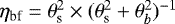 ; θs and θb are the source and the beam sizes (both assumed to be a circular Gaussian).
All Tables
Results of the spectral fit of the hyperfine components performed using the GILDAS-CLASS tool: sum of the opacities, line width, and peak velocity.
Number of detected lines (S∕N ≥ 3), range of upper level energies of the detected transitions, temperatures (K), and beam-averaged column densities (cm−2) derived from the rotational diagram analysis.
Source-averaged molecular column density (Ntot), gas physical conditions (temperature, Tkin, and density, nH_2), source size inferred from the LVG analysis, and beam-filling factor (ηbf) of c-C3H2, CH3OH, and CH3CN lines towards the four protostars in our sample (L1489-IRS, B5-IRS1, L1455-IRS1, and L1551-IRS5).
Upper limits (3σ) on the column densities of the iCOMs detected in L1551-IRS5 towards L1489-IRS, B5-IRS1, and L1455-IRS1.
Abundance ratios of the deuterated molecule to the non-deuterated molecule and inferred D/H ratios in the observed Class I sources.
L1489-IRS: Temperatures and beam-averaged col- umn densities derived for the envelope (see text).
B5-IRS1: Temperatures and beam-averaged column densities for different physical components (envelope, outflow; see text).
L1455-IRS1: Temperatures and beam-averaged column densities for different physical components (envelope, out- flow; see text).
L1551-IRS5: Temperatures and beam-averaged column densities for different physical components (envelope, out- flow, and hot corino; see text).
All Figures
|
Fig. 1 Spectra observed in the 214 500–222 200 MHz and 230 200–238 000 MHz range towards L1489–IRS, B5–IRS1, L1455–IRS1, and L1551–IRS5, ordered from top to bottom according to the number of detected lines (see Table 4). Labels of selected detected species (see Sect. 4.1, Figs. A.1–A.4, and Tables A.1–A.4) are reported. |
| In the text | |
|
Fig. 2 Histogram of the numbers of detected lines for iCOMs (pink), C-chains (green), S-bearing molecules (blue) for the four protostars in our sample (ordered by increasing number of detected species). |
| In the text | |
|
Fig. 3 Result of the LVG analysis for L1551-IRS5. The inferred range of gas density and temperature are summarized in Table 6. χ2 contour plots as a function of the gas density and temperature. The green and pink contours show the 1σ confidence level for CH3OH and CH3CN, respectively, for representative value of N(CH3OH) = 5 × 1018 cm−2 with source size of 0.′′18 and N(CH3CN) ≥ 1 × 1017 cm−2 with source size of 0.′′11. |
| In the text | |
|
Fig. 4 Ratios of the observed line intensities to those predicted by the best-fitting LVG models as a function of upper level energy of the considered transitions towards L1551-IRS5. Upper panel: blue and red circles are for the ortho and para c-C3H2, respectively. Middle panel: Blue and red stars show the E and A transitions of CH3OH, respectively. Bottom panel: blue and red diamonds are for the E and A CH3CN lines, respectively. |
| In the text | |
|
Fig. 5 Normalized intensity profiles of selected species towards L1489-IRS, B5-IRS1, L1455-IRS1, and L1551-IRS5. The profiles of SO, c-C3H2, H2CO (in all sources), CH3OH, CH3CHO, HCOOCH3 (in L1551-IRS5), and OCS (in L1455-IRS1) were obtained by stacking the detected transitions for each species in order to maximize the S/N. CH3OH (4−2,3 –3−1,2E) in B5-IRS1 and L1455-IRS1 is the transition at 218 440 MHz; H2CS (71,7 –61,6) in B5-IRS1, L1455-IRS1, and L1551-IRS5 is the transition at 236 727 MHz; H2S (22,0 –21,1) in L1455-IRS1 and L1551-IRS5 is the transition at 216 710 MHz; OCS (19–18) in L1551-IRS5 is the transition in 231 060 MHz. |
| In the text | |
|
Fig. 6 Correlation of the column densities of CH3OH and c-C3H2 towards the four protostars in our sample. The sources are labeled in the legend in the bottom right corner. The dashed lines indicate a CH3OH/c-C3H2 column density ratio of 100, 10, and 1. |
| In the text | |
|
Fig. 7 Normalized intensity profiles of four species towards L1551-IRS5. The spectra of CH3OH in green and c-C3H2 in pink in the upper panel are obtained after stacking the detected transitions (see Fig. 5). The spectra of H2S in blue and OCS in red in the lower panel are transitions 22,0–21,1 and 19–18, respectively (see Fig. A.4). The dashed and dash-dotted lines represent the systemic velocities of the southernprotostar (4.5 km s−1) and the northern protostar (7.5 km s−1), respectively (Bianchi et al. 2020), while the dotted line represents the systemic velocity of the circumbinary envelope (6.4 km s−1) measured using the C18O 2–1 line (this work). |
| In the text | |
|
Fig. 8 Abundance ratios [XD]/[XH] measured for organic species in sources at different evolutionary stages: prestellar cores (D2CO (Bacmann et al. 2003; Chacón-Tanarro et al. 2019), CH2DOH (Bizzocchi et al. 2014; Chacón-Tanarro et al. 2019; Ambrose et al. 2021), and HDCS (Marcelino et al. 2005; Vastel et al. 2018)); Class 0 protostars (D2CO (Parise et al. 2006; Watanabe et al. 2012; Persson et al. 2018; Manigand et al. 2020), CH2DOH (Parise et al. 2006; Bianchi et al. 2017b; Jørgensen et al. 2018; Jacobsen et al. 2019; van Gelder et al. 2020; Manigand et al. 2020), and HDCS (Drozdovskaya et al. 2018); Class I protostars (SVS13-A; D2CO, CH2DOH (Bianchi et al. 2017a), and HDCS (Bianchi et al. 2019a)); comets (Hale-Bopp; CH2DOH (Crovisier et al. 2004) and 67P/C-G; CH2DOH (Drozdovskaya et al. 2021)). The [XD]/[XH] values inferred for L1489-IRS, B5-IRS1, L1455-IRS1, and L1551-IRS5 are in magenta (from this work). The dashed bars represent values inferred for the hot corinos (r ≤ 100 au, T ≥ 100 K), while the filled bars indicate the measurements derived for extended envelope. |
| In the text | |
|
Fig. 9 Abundance ratios of organic molecules towards the four protostars. Upper panel: abundance ratios of iCOMs with respect to methanol measured at different evolutionary stages. The three panels (from left to right) refer to CH3CN, CH3CHO, and HCOOCH3, and each is divided into four parts; the gray dashed lines separate the Class 0 sources, Class I sources, protoplanetary disks (PPD), and comets. The abundance ratios estimated for L1551-IRS5 in this work are indicated by a magenta circle. The abundance ratios for the literature sources (see text for references) are labeled in the legend in the bottom right corner. Bottom panels: abundance ratios of [CH3OH]/[H2CO] (left) and [H2CS]/[H2CO] (right) for our Class I sources (magenta bars) compared with the values of prestellar cores, Class 0 sources, PPDs, and comets from the literature, as labeled. The dashed bar in the left panel indicates hot corino measurements, while the dashed bar in the right panel indicates the measurement obtained in the inner 60 au towards the IRAS 16293B protostar. The references of the measurements from the literature are reported in Sect. 5.3.2. |
| In the text | |
|
Fig. A.1 Spectra observed towards L1489-IRS (see Table A.1 in TMB scale). Species, transition, and upper level energy are reported in each panel. The vertical dashed line stands for the source systemic velocity measured using the C18O(2–1) line (+7.3 km s−1). In the CCD(3–2) spectrum the velocity scale is centered on the brightest (3 D2) hyperfine component (vertical blue line) at 216372.8 MHz; the vertical red lines indicate the offset in velocity of the fainter components (1.9 D2 at 216373.3 MHz; 1.4 D2 at 216373.2 MHz. This spectrum is smoothed to 0.40 MHz. In the C15N(2–1) spectrum (lower panel) the velocity scale is centered on the brightest (6 D2) hyperfine component (vertical blue line) at 219934.8 MHz; the vertical red line indicates the offset in velocity of the fainter components (4 D2 at 219934.0 MHz). In the DCN(3–2) spectrum the velocity scale is centered on the brightest (35 D2) hyperfine component (vertical blue line) at 217238.3 MHz; the vertical red lines indicate the offset in velocity of the fainter components (20 D2 at 217238.6 MHz; 16 D2 at 217238.3 MHz). |
| In the text | |
|
Fig. A.2 Spectra observed towards B5-IRS1 (see Table A.2 in TMB scale). Species, transition, and upper level energy are reported in each panel. The vertical dashed line stands for the source systemic velocity measured using the C18O(2–1) line (+10.2 km s−1). In the 13CN(2–1) spectrum the velocity scale is centered on the brightest (8 D2) hyperfine component (vertical blue line) at 217467.1 MHz; the vertical red line indicates the offset in velocity of the fainter component (5 D2 at 217467.1 MHz). In the 13CS(5–4) spectrum the velocity scale is centered on the brightest (38 D2) hyperfine component (vertical blue line) at 231220.7 MHz; the vertical red lines indicate the offset in velocity of the fainter components (21 D2 at 231220.7 MHz; 17 D2 at 231220.6 MHz; 1 D2 at 231220.5 MHz). In the CCD(3–2) spectrum (middle panel, middle column) the velocity scale is centered on the brightest (3 D2) hyperfine component (vertical blue line) at 216372.8 MHz; the vertical red lines indicate the offset in velocity of the fainter components (1.9 D2 at 216373.3 MHz; 1.4 D2 at 216373.2 MHz). Lower panel: In the CCD(3–2) spectrum the velocity scale is centered on the brightest (2 D2) hyperfine component (vertical blue line) at 216428.3 MHz; the vertical red line indicate the offset in velocity of the fainter components (0.7 D2 at 216428.8 MHz). In the DCN(3–2) spectrum the velocity scale is centered on the brightest (35 D2) hyperfine component (vertical blue line) at 217238.3 MHz; the vertical red lines indicates the offset in velocity of the fainter components (20 D2 at 217238.6 MHz; 16 D2 at 217238.3 MHz). |
| In the text | |
|
Fig. A.2 Continued: Spectra observed towards B5-IRS1 (see Table A.2 in TMB scale). In theo- c-C3H2 spectrum the velocity scale is centered on the brightest (63 D2) hyperfine component (vertical blue line) at 218449.4 MHz; the vertical red line indicates the offset in velocity of the fainter components (21 D2 at 216448.8 MHz). The CH2DOH spectrum is smoothed to 0.40 MHz. |
| In the text | |
|
Fig. A.3 Spectra observed towards L1455-IRS1 (see Table A.3 in TMB scale). Species, transition, and upper level energy are reported in each panel. The vertical dashed line stands for the source systemic velocity measured using the C18O(2–1) line (+4.7 km s−1). In the 13CN(2–1) spectrum the velocity scale is centered on the brightest (8 D2) hyperfine component (vertical blue line) at 217467.1 MHz; the vertical red line indicates the offset in velocity of the fainter component (5 D2 at 217467.1 MHz). In the 13CS(5–4) spectrum the velocity scale is centered on the brightest (38 D2) hyperfine component (vertical blue line) at 231220.7 MHz; the vertical red lines indicate the offset in velocity of the fainter components (21 D2 at 231220.7 MHz; 17 D2 231220.6 MHz; 1 D2 at 231220.5 MHz). In the CCD(3–2) spectrum (fourth row) the velocity scale is centered on the brightest (2 D2) hyperfine component (vertical blue line) at 216428.3 MHz; the vertical red line indicates the offset in velocity of the fainter components (0.7 D2 at 216428.8 MHz). Lower panel: In the CCD(3–2) spectrum the velocity scale is centered on the brightest (3 D2) hyperfine component (vertical blue line) at 216372.8 MHz; the vertical red lines indicate the offset in velocity of the fainter components (1.9 D2 at 216373.3 MHz; 1.4 D2 at 216373.2 MHz). In the DCN(3–2) spectrum the velocity scale is centered on the brightest (35 D2) hyperfin component (vertical blue line) at 217238.3 MHz; the vertical red lines indicate the offset in velocity of the fainter components (20 D2 at 217238.6 MHz; 16 D2 at 217238.3 MHz). |
| In the text | |
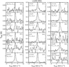 |
Fig. A.3 Continued: Spectra observed towards L1455-IRS1 (see Table A.3 in TMB scale). |
| In the text | |
|
Fig. A.4 Spectra observed towards L1551-IRS5 (see Table A.4 in TMB scale). Species, transition, and upper level energy are reported in each panel. The vertical dotted line stands for the source systemic velocity as measured using the C18O(2–1) line (+6.4 km s−1). The vertical dashed line and the vertical dash-dotted line stand for the systemic velocities of the binary system associated with the southern source (+4.5 km s−1) and northern source (+7.5 km s−1), respectively. In the 13CS(5–4) spectrum the velocity scale is centered on the brightest (38 D2) hyperfine component (vertical blue line) at 231220.7 MHz; the vertical red lines indicate the offset in velocity of the fainter components (21 D2 at 231220.7 MHz; 17 D2 at 231220.6 MHz; 1 D2 at 231220.5 MHz). In the C15N(2–1) spectrum (lower panel) the velocity scale is centered on the brightest (6 D2) hyperfine component (vertical blue line) at 219934.8 MHz; the vertical red lines indicate the offset in velocity of the fainter components (4 D2 at 219934.0 MHz). |
| In the text | |
|
Fig. A.4 Continued: Spectra observed towards L1551-IRS5 (see Table A.4 in TMB scale). Lower left panel of the first column: In the CCD(3–2) spectrum the velocity scale is centered on the brightest (2 D2) hyperfine component (vertical blue line) at 216428.3 MHz; the vertical red lines indicate the offset in velocity of the fainter components (0.3 D2 at 216430.3 MHz; 0.7 D2 at 216428.8 MHz). Upper middle panel: In the CCD(3–2) spectrum the velocity scale is centered on the brightest (3 D2) hyperfine component (vertical blue line) at 216372.8 MHz; the vertical red lines indicate the offset in velocity of the fainter components (1.9 D2 at 216373.3 MHz; 1.4 D2 at 216373.2 MHz). In the DCN(3–2) spectrum the velocity scale is centered on the brightest (35 D2) hyperfine component (vertical blue line) at 217238.3 MHz; the vertical red lines indicate the offset in velocity of the fainter components (20 D2 at 217238.6 MHz; 16 D2 at 217238.3 MHz). In the N2D+ spectrum the velocity scale is centered on the brightest (312 D2) hyperfine component (vertical blue line) at 231319.9 MHz; the vertical red line indicates the offset in velocity of the brightest transition of 40 fainter components (5 D2 at 231324.5 MHz). |
| In the text | |
|
Fig. A.4 Continued: Observed spectra observed towards L1551-IRS5 (see Table A.4 in TMB scale). In thec-C3H(41,3–31,2) spectrum the velocity scale is centered on the c-C3H2 emission (vertical blue line) at 216492.6 MHz; the vertical red line indicates possible contamination due to D2CO(81,7–81,8) at 216492.4 MHz. In the H2C33S(71,7–61,6) spectrum the velocity scale is centered on the brightest (67 D2) hyperfine component (vertical blue line) at 234678.8 MHz; the vertical red lines indicate the offset in velocity of the fainter components (58 D2 at 234678.7 MHz; 2 D2 234676.9 MHz). |
| In the text | |
|
Fig. A.4 Continued: Observed spectra of the molecules, towards L1551-IRS5, listed in Table A.4 (in TMB scale). In theo-c-C3H2 spectrum the velocity scale is centered on the brightest (63 D2) hyperfine component (vertical blue line) at 218449.4 MHz; the vertical red lines indicate the offset in velocity of the fainter components (21 D2 at 216448.8 MHz). In the CH3OH spectrum the velocity scale is centered on the CH3OH emission at 231281.1 MHz; the vertical red line indicates possible contamination due to CH3CHO at 231278.5 MHz. |
| In the text | |
|
Fig. A.4 Continued: Observed spectra of the molecules, towards L1551-IRS5, listed in Table A.4 (in TMB scale). In theCH3CCH spectrum the velocity scale is centered on the CH3CCH emission at 222128.8 MHz; the vertical red line indicates possible contamination due to HCOOCH3 at 222128.2 MHz. In the three HCOOCH3 spectra the spectra are centered on the brightest component (vertical blue line) and the vertical red lines indicate the offset in velocity and strength of the fainter components reported in Table A.4. |
| In the text | |
|
Fig. A.5 Observed spectra of CO isotopologues (in TMB scale) towards L1489-IRS (left column) and B5-IRS1 (right column). Species, transition, and upper level energy are reported in each panel. For the panels in the left column the vertical dashed lines stand for the source systemic velocity as measured using C18O (2-1) emission (+7.3 km s−1). For the panels in the right column the vertical dashed lines stand for the source systemic velocity measured using C18O (2-1) emission (+10.2 km s−1). Top panels: CO (2-1) transition. Middle panels: Zoom-in on the CO (2-1) line wings (in black) and the 13CO (2-1) line wings (in magenta), scaled by a factor of 77 in the TMB range from -2 K to 2.5 K. Bottom panels: 13CO (in green) and C18O (in red) scaled by a factor of 7.27 assuming isotopic ratios of 12C/13C = 77 and 16O/18O = 560 (Milam et al. 2005). |
| In the text | |
|
Fig. A.6 Observed spectra of CO isotopologues (in TMB scale) towards L1455-IRS1 (left column) and L1551-IRS5 (right column). Species, transition, and upper level energy are reported in each panel. For the panels in the left column the vertical dashed lines stand for the source systemic velocity as measured using C18O (2-1) emission (+4.7 km s−1). For the panels in the right column the vertical dotted line stands for the source systemic velocity measured using the C18O(2–1) line (+6.4 km s−1). The vertical dashed line and the vertical dash-dotted line stand for the systemic velocities of the binary system associated with the southern source (+4.5 km s−1) and northern source (+7.5 km s−1) respectively.Top panels: CO (2-1) transition. Middle panels: Zoom-in on the CO (2-1) line wings (in black) and the 13CO (2-1) line wings (in magenta), scaled by a factor of 77 in the TMB range from -2 K to 2.5 K. Bottom panels: 13CO (in green) and C18O (in red) scaled by a factor of 7.27 assuming isotopic ratios of 12C/13C = 77 and 16O/18O = 560 (Milam et al. 2005). |
| In the text | |
|
Fig. B.1 Rotational diagrams of SO, H2CO, and c-C3H2 in L1489-IRS. The parameters Nup, gup, and Eup are respectively the column density, the degeneracy, and the energy (with respect to the ground state of each symmetry) of the upper level. The error bars include the errors on the flux, as stated in Table A.1, and the uncertainty of the calibration of 20%. |
| In the text | |
|
Fig. B.2 Rotational diagrams of SO, H2CO, and c-C3H2 in B5-IRS1. The parameters Nup, gup, and Eup are respectively the column density, the degeneracy, and the energy (with respect to the ground state of each symmetry) of the upper level. The error bars include the errors on the flux, as stated in Table A.2, and the uncertainty of the calibration of 20%. |
| In the text | |
|
Fig. B.3 Rotational diagrams of SO, OCS, HDCS, H2CO, and c-C3H2 in L1455-IRS1. The parameters Nup, gup, and Eup are respectively the column density, the degeneracy, and the energy (with respect to the ground state of each symmetry) of the upper level. The error bars include the errors on the flux, as stated in Table A.3, and the uncertainty of the calibration of 20%. |
| In the text | |
|
Fig. B.4 Rotational diagrams of SO, SO2, OCS, H2CO, D2CO, H2CCO, c-C3H2, CH3OH, CH3CN, CH3CCH, and CH3CHO. The parameters Nup, gup, and Eup are respectively the column density, the degeneracy, and the energy (with respect to the ground state of each symmetry) of the upper level. The derived values of the rotational temperature and the column density are reported in each panel for each species. For D2CO the blue and red circles indicate ortho and para transitions, respectively. For CH3OH the blue and red circles indicate E and A transitions, respectively. Red stars in the c-C3H2 (83,6 – 82,7) and CH3OH (102,9 – 93,6) indicate transitions not used in the fit, due to contamination by other molecules. The blue arrow in the CH3CN panel indicates 124 – 114 transition, which was not used in the fit as upper limit. The error bars include the errors on the flux, as stated in Table A.4, and the uncertainty of the calibration of 20%. |
| In the text | |
Current usage metrics show cumulative count of Article Views (full-text article views including HTML views, PDF and ePub downloads, according to the available data) and Abstracts Views on Vision4Press platform.
Data correspond to usage on the plateform after 2015. The current usage metrics is available 48-96 hours after online publication and is updated daily on week days.
Initial download of the metrics may take a while.