| Issue |
A&A
Volume 657, January 2022
|
|
|---|---|---|
| Article Number | A2 | |
| Number of page(s) | 22 | |
| Section | Cosmology (including clusters of galaxies) | |
| DOI | https://doi.org/10.1051/0004-6361/202142340 | |
| Published online | 20 December 2021 | |
Turbulent magnetic fields in the merging galaxy cluster MACS J0717.5+3745⋆
1
Dipartimento di Fisica e Astronomia, Universitá di Bologna, Via P. Gobetti 93/2, 40129 Bologna, Italy
e-mail: This email address is being protected from spambots. You need JavaScript enabled to view it.
2
INAF-Istituto di Radio Astronomia, Via Gobetti 101, 40129 Bologna, Italy
3
Thüringer Landessternwarte (TLS), Sternwarte 5, 07778 Tautenburg, Germany
4
Hamburger Sternwarte, Universität Hamburg, Gojenbergsweg 112, 21029 Hamburg, Germany
5
Leiden Observatory, Leiden University, PO Box 9513 2300 RA Leiden, The Netherlands
6
Minnesota Institute for Astrophysics, University of Minnesota, 116 Church St. S.E., Minneapolis, MN 55455, USA
7
Molecular Foundry, Lawrence Berkeley National Laboratory, Berkeley, CA 94720, USA
8
Harvard-Smithsonian Center for Astrophysics, 60 Garden Street, Cambridge, MA 02138, USA
9
CSIRO Astronomy and Space Science, PO Box 1130 Bentley, WA 6102, Australia
10
Astronomy and Astrophysics Division, Physical Research Laboratory, Ahmedabad 380009, India
11
Department of Physics, School of Natural Sciences UNIST, Ulsan 44919, Korea
12
INAF-Osservatorio Astronomico di Cagliari, Via della Scienza 5, 09047 Selargius, CA, Italy
13
Department of Physics, New Mexico Tech, Socorro, NM 87801, USA
14
National Radio Astronomy Observatory, Socorro, NM 87801, USA
15
US Naval Research Laboratory, 4555 Overlook Avenue SW, Washington, DC 20375, USA
Received:
30
September
2021
Accepted:
27
October
2021
Abstract
We present wideband (1 − 6.5 GHz) polarimetric observations, obtained with the Karl G. Jansky Very Large Array, of the merging galaxy cluster MACS J0717.5+3745, which hosts one of the most complex known radio relic and halo systems. We used both rotation measure synthesis and QU-fitting to find a reasonable agreement of the results obtained with these methods, particularly when the Faraday distribution is simple and the depolarization is mild. The relic is highly polarized over its entire length (850 kpc), reaching a fractional polarization > 30% in some regions. We also observe a strong wavelength-dependent depolarization for some regions of the relic. The northern part of the relic shows a complex Faraday distribution, suggesting that this region is located in or behind the intracluster medium (ICM). Conversely, the southern part of the relic shows a rotation measure very close to the Galactic foreground, with a rather low Faraday dispersion, indicating very little magnetoionic material intervening along the line of sight. Based on a spatially resolved polarization analysis, we find that the scatter of Faraday depths is correlated with the depolarization, indicating that the tangled magnetic field in the ICM causes the depolarization. We conclude that the ICM magnetic field could be highly turbulent. At the position of a well known narrow-angle-tailed galaxy (NAT), we find evidence of two components that are clearly separated in the Faraday space. The high Faraday dispersion component seems to be associated with the NAT, suggesting the NAT is embedded in the ICM while the southern part of the relic lies in front of it. If true, this implies that the relic and this radio galaxy are not necessarily physically connected and, thus, the relic may, in fact, not be powered by the shock re-acceleration of fossil electrons from the NAT. The magnetic field orientation follows the relic structure indicating a well-ordered magnetic field. We also detected polarized emission in the halo region; however, the absence of significant Faraday rotation and a low value of Faraday dispersion suggests the polarized emission that was previously considered as the part of the halo does, in fact, originate from the shock(s).
Key words: galaxies: clusters: general / radiation mechanisms: non-thermal / polarization / acceleration of particles / magnetic fields / large-scale structure of Universe
The reduced images are only available at the CDS via anonymous ftp to cdsarc.u-strasbg.fr (130.79.128.5) or via http://cdsarc.u-strasbg.fr/viz-bin/cat/J/A+A/657/A2
© ESO 2021
1. Introduction
Magnetic fields are pervasive throughout the Universe and play a vital role in numerous astrophysical processes: from our solar system up to filaments and voids in the large-scale structure (e.g., Klein & Fletcher 2015; Beck 2015). Even the largest virialized structures in the Universe, namely, galaxy clusters, are permeated by magnetic fields (see Carilli & Taylor 2002; Govoni & Feretti 2004; Donnert et al. 2018, for reviews). However, the actual strength, topology, and evolution of these fields is poorly constrained.
The strongest evidence of cluster-wide magnetic fields comes from radio observations that have revealed large megaparsec-size, diffuse synchrotron emitting sources known as radio relics and halos (see van Weeren et al. 2019, for a recent review). The presence of large-scale magnetic fields may have important implications for the different processes observed in galaxy clusters. A detailed analysis of the diffuse radio sources in clusters may help to shed light on the origin of the magnetic fields, for example, to determine whether very weak seed fields are amplified by a dynamo process in the intracluster medium (ICM) as well as to determine how the magnetic fields impact the physics of the ICM.
Radio relics are found in the periphery of merging galaxy clusters and they often show irregular and filamentary morphologies (e.g., Owen et al. 2014; van Weeren et al. 2017b; Rajpurohit et al. 2018; Di Gennaro et al. 2018; Rajpurohit et al. 2020a). Relics trace shock waves occurring in the ICM during cluster merger events (e.g., Sarazin et al. 2013; Ogrean et al. 2013; van Weeren et al. 2016a; Botteon et al. 2016, 2018).
It is believed that the cosmic ray electrons (CRe), which form the radio relics via synchrotron emission, originate from a first-order Fermi process, namely, diffusive shock acceleration (DSA, e.g., Blandford & Eichler 1987; Drury 1983; Ensslin et al. 1998; Hoeft & Brüggen 2007). The DSA at the shocks causing relics may also re-accelerate a pool of mildly relativistic fossil electrons, previously injected by active galactic nuclei (AGN: e.g., Bonafede et al. 2014; van Weeren et al. 2017a). The existence of mildly relativistic electrons in front of the shock may help to reconcile the low acceleration efficiency with the high radio luminosity for relics with weak shocks (Mach number ≤2, e.g., Kang & Ryu 2011; Botteon et al. 2020). However, the exact spectral energy distribution and spatial distribution of such fossil electrons in the ICM are mostly unconstrained.
Radio relics are strongly polarized at frequencies above 1 GHz, some with a polarization fraction as high as 65% (e.g., van Weeren et al. 2010, 2012; Owen et al. 2014; Kierdorf et al. 2017; Loi et al. 2020; Rajpurohit et al. 2020b; Di Gennaro et al. 2021). The inferred magnetic field directions are often found to be well aligned with the shock surface. However, the exact mechanism causing the high degree of polarization and the aligned polarization angle is still unclear. The alignment could be caused by a preferentially tangential magnetic field orientation or by the compression of a small-scale tangled magnetic field at the shock (Laing 1980; Ensslin et al. 1998).
Unlike relics, radio halos are typically unpolarized sources located at the center of a cluster. The radio emission from halos roughly follows the X-ray emission (e.g., Pearce et al. 2017; Rajpurohit et al. 2018; van Weeren et al. 2017a). The scenario that is currently favored for the formation of radio halos involves the reacceleration of CRe to higher energies as a result of turbulence induced during mergers (e.g., Brunetti et al. 2001; Petrosian 2001; Brunetti & Jones 2014).
Polarized emission at the cluster outskirts is crucial for understanding the magnetic field properties of the ICM (see, Carilli & Taylor 2002; Govoni & Feretti 2004, for a review). The orientation and topology of magnetic fields at merger shocks is important in better understanding the physics of shock acceleration because the efficiency of particle acceleration might be a strong function of the magnetic field topology upstream of the shock (e.g., Wittor et al. 2020). However, magnetic fields in the ICM are notoriously difficult to measure and the low-density regions in the cluster outskirts are even more challenging to probe (Johnson et al. 2020).
In this work, we describe the results obtained from polarimetric analysis of Karl G. Jansky Very Large Array (VLA) L-, S-, and C-band observations covering the 1–6.5 GHz frequency range. The enormous scope of wideband data and remarkable resolution allow us to carry out spatially resolved polarimetric studies, providing crucial insights into the ICM magnetic fields.
The outline of this paper is as follows: in Sect. 3, we describe the observations and data reduction. The polarization images are presented in Sect. 4. This is followed by a detailed analysis and discussion from Sects. 5 to 12. We summarize our main findings in Sect. 13.
Throughout this paper, we assume a ΛCDM cosmology with H0 = 70 km s−1 Mpc−1, Ωm = 0.3, and ΩΛ = 0.7. At the cluster’s redshift, 1″ corresponds to a physical scale of 6.4 kpc. All output images are in the J2000 coordinate system and are corrected for primary beam attenuation.
2. MACS J0717.5+3745
The galaxy cluster MACS J0717.5+3745 (l = 180.25° and b = +21.05°) located at z = 0.5458, hosts one of the most complex and powerful known relic-halo systems. (e.g., Bonafede et al. 2009; van Weeren et al. 2009, 2017b; Pandey-Pommier et al. 2013; Rajpurohit et al. 2021a,c). The relic consists of four subregions, which have historically been referred to as R1, R2, R3, and R4; see Fig. 1. The relic is known to be polarized above 1.4 GHz and the polarization fraction varies along the relic (Bonafede et al. 2009).
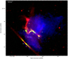 |
Fig. 1. Composite total power, polarization intensity, and X-ray image of the relic in MACS J0717+3745 at 2″ resolution. The total power and L-band polarization emission are shown in red and green-yellow, respectively. The intensity in blue shows the X-ray emission. The lack of polarized emission in the north region (R1) indicates depolarization. The image properties are given in Table 1, IM5 and IM9. |
High-resolution images from the VLA reveal that the relic has several filaments on scales down to 30 kpc. Some of these filaments originate from the relic itself, while a few of them, namely, F1 and F2 (see Fig. 1), appear more isolated. Recently, it was reported that the relic consists of several fine overlapping structures with different spectral indices (Rajpurohit et al. 2021c). The curvature distribution suggests that the relic is very likely seen less edge-on with a viewing angle close to about 45°.
At the center of the relic, there is an embedded Narrow Angle Tail (NAT) galaxy (see Fig. 1). At high frequencies (above 1 GHz), the tails of the NAT seem to fade into the R3 region of the relic (van Weeren et al. 2017b). However, at low frequencies (below 750 MHz), the tails are apparently bent to the south of the R3 region (Rajpurohit et al. 2021c). It is not clear whether this morphological connection between the NAT and the relic is physical or they are simply two different structures projected along the same line of sight (van Weeren et al. 2017b; Rajpurohit et al. 2021c). If this connection is physical, it may suggest that the relic is powered by the shock re-acceleration of mildly relativistic fossil electrons from the NAT.
The cluster also hosts a powerful steep spectrum radio halo with a largest linear size of about 2.6 Mpc (Bonafede et al. 2009, 2018; van Weeren et al. 2009, 2017b; Pandey-Pommier et al. 2013; Rajpurohit et al. 2021a). High-resolution total power images taken with the VLA have shown the presence of several radio filaments of 100–300 kpc located within the halo region (van Weeren et al. 2017b). The halo in MACS J0717.5+3745 has previously been reported to be polarized at the level of 2–7% at 1.4 GHz (Bonafede et al. 2009), which is uncommon for radio halos. However, it is unclear if the reported polarized emission is truly associated with the halo or not.
3. Observations and data reduction
VLA wideband observations of MACS J0717.5+3745 were obtained in L-band (ABCD-array configuration), S-band (ABCD-array configuration), and C-band (BCD-array configuration), covering the frequency range from 1 to 6.5 GHz. For observation details and a description of the data reduction procedure, we refer to van Weeren et al. (2016b, 2017b). While previous analyses of the data only considered the total power, the VLA observations were taken in full-polarization mode, allowing us to investigate the polarization properties of the cluster.
The data reduction and imaging were performed with CASA. The data were calibrated for antenna position offsets, elevation-dependent gains, parallel-hand delay, bandpass, and gain variations using 3C147. For polarization calibration, the leakage response was determined using the unpolarized calibrator 3C147. The cross-hand delays and the absolute polarization position angle were corrected using 3C138. Finally, the calibration solutions were applied to the target field and the resulting calibrated data were averaged by a factor of 4 in frequency per spectral window. Several rounds of self-calibration were performed to refine the gain solutions. After the individual data sets were calibrated, the observations from the different configurations (for the same frequency band) were combined and imaged together.
We produced Stokes I, Q, and U images of the target field from the data at L-band, S-band, and C-band, including data from all array configurations. Deconvolution was done with CLEAN masks generated in the PyBDSF (Mohan & Rafferty 2015). Imaging was always performed with Briggs weighting (Briggs 1995) using robust = 0.0 and all images were corrected for primary beam attenuation, see Table 1 for the properties of the images obtained. For Faraday analysis, the full 1–6.5 GHz channel with Stokes IQU cubes were imaged to a common resolution of 4″, 5″, and 12.5″. These IQU cubes were inspected and any spectral channels that showed large artifacts or a large increase in noise compared to the average were excluded. We note that the highest common resolution possible with our L-, S-, and C-bands VLA data was 4″; therefore 2″ resolution Stokes IQU cubes were not used for the Faraday analysis.
Image properties.
The polarized flux density was computed from the Stokes Q and U flux densities according to the definition of polarization as a complex property:
 (1)
(1)
where the absolute of P results in the polarized flux density. Since both Q and U are affected by noise in the measurement, we correct the polarized flux density, |P|, for the Rician bias (Wardle & Kronberg 1974; George et al. 2012) to:
 (2)
(2)
where σQU is the average rms of Stokes Q and U images and the index “meas” indicates the measured property, unavoidably including a noise, for clarity. The uncertainties in the flux density measurements are estimated as:
 (3)
(3)
where f is an absolute flux density calibration uncertainty, Sν is the flux density, σrms is the root mean square (RMS) noise, and Nbeams is the number of beams covered by the source. We assume absolute flux density uncertainties of 4% for the VLA L-band and 2.5% for the VLA S- and C-bands (Perley & Butler 2013).
4. Polarized emission
In Fig. 2, we show the high-resolution (2″) polarized intensity maps of the relic for the VLA L-, S-, and C-bands. Polarized emission from the relic subregions (R1, R2, R3, and R4) was detected in all three frequency bands.
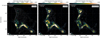 |
Fig. 2. Polarization intensity images of the relic in MACS J0717.5+3745 at 2″ resolution, showing that the polarization emission is distributed in a clumpy manner. The image also revels fine, small-scale filaments visible in the total power emission. Contour levels are drawn at |
![Mathematical equation: $ \sqrt{[1,2,4,8,\dots]}\,\times\,5\sigma_{{\mathrm{rms}}} $](/articles/aa/full_html/2022/01/aa42340-21/aa42340-21-eq5.gif)
The polarized emission more or less follows the structure seen in the total intensity images; however, the polarized emission seems to be more “clumpy” compared to the total power emission. Moreover, we find that there are fluctuations in the polarization intensity, particularly for the northern part of the relic (R1 and R2), on a scale as small as 10 kpc. The polarized intensity map in Fig. 2 also indicates that in L-band the polarized flux density in the northern part of the relic is low compared to the southern part (R3 and R4). To investigate this further, we created maps for the fractional polarization p = |P|/I.
The L-, S-, and C-band high-resolution (2″) fractional polarization maps of the relic are shown in Fig. 3. At such a high resolution, the relic is polarized over its entire length in C-band. We find that in all three bands, the polarization fraction across the relic varies significantly, from unpolarized to a maximum fractional polarization of about 50% in C-band.
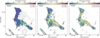 |
Fig. 3. High-resolution (2″) fractional polarization maps at VLA L-, S-, and C-bands. The relic is polarized at all of the observed frequencies, reaching values up to 50% in some regions. The northern part of the relic strongly depolarizes at 1.5 GHz. Contour levels are drawn at |
![Mathematical equation: $ \sqrt{[1,2,4,8,\dots]}\,\times\,5\sigma_{{\mathrm{rms}}} $](/articles/aa/full_html/2022/01/aa42340-21/aa42340-21-eq6.gif)
An overview of the polarization properties of the diffuse radio sources in the cluster is given in Table 2. We measured the average fractional polarization in the four subregions of the relic. These regions are shown in the left panel of Fig. 4. The spatially averaged polarization fraction over R1 is (21 ± 2)% in C-band. The fractional polarization drops quickly towards lower frequencies, reaching as low as (3 ± 1)% in L-band. Similar trends are noticed for the R2 region of the relic. We observe large local fluctuations in the polarization fraction, in particular for R1 and R2.
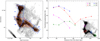 |
Fig. 4. Left: VLA L-band image depicting regions used for flux density extraction and RM-synthesis and QU-fitting. Blue regions show the relic subregions where the average fractional polarization was extracted. The fractional polarization at R3 in Table 2 is obtained by excluding the contribution from the NAT. Red boxes where flux densities and Faraday dispersion functions were extracted for QU-fitting and RM-synthesis, respectively. Each red box has a width of 5″, corresponding to a physical size of 32 kpc. Right: fractional polarization profiles across the relic extracted from the rectangular regions, depicted in the inset, of width 2″. There is a hint that the fractional polarization decreases in the downstream regions (i.e., shown with arrows). |
Polarization properties of the diffuse radio emission in the cluster MACS J0717.5+3745.
From Table 2, the average fractional polarization of the R3 region ((28 ± 3)% at C-band) is highest compared to the rest of the relic. In the region where the NAT is located, we find a very low fractional polarization in all three bands. For the relic, the average polarization fraction at R4 is the lowest (15 ± 1% at C-band).
In the right panel of Fig. 4, we show the polarization fraction profiles for the relic extracted from the 2″ map at 3 GHz. The corresponding regions are depicted in the inset. Overall, there is a hint that the fractional polarization decreases in the downstream regions. Recently, Di Gennaro et al. (2021) found that the polarization fraction decreases toward the downstream of the entire Sausage relic. Simulations show that such trends are expected in a turbulent medium while opposite trends (i.e., polarization fraction increasing toward the downstream region of a shock front) is expected if the medium is uniform (Domínguez-Fernández et al. 2021). In the R2 region of the relic, the degree of polarization first decreases for about 60 kpc and then increases (from 60 kpc to 100 kpc). This could be due to projection effects because there are filamentary structures at that location (van Weeren et al. 2017b).
Looking at the high-resolution fractional polarization images from C-band to L-band (Fig. 3), the average fractional polarization of the relic in MACS J0717.5+3745 also increases in L-band and S-band from R1 to R3. We find that the degree of polarization decreases generally with increasing wavelength.
We also create polarization maps at 5″ resolution. The resulting maps at 1.5 GHz, 3 GHz, and 5.5 GHz are shown in Fig. 5. We note that that these polarization intensity maps are obtained by applying the rotation measure synthesis (RM-synthesis: Brentjens & de Bruyn 2005, discussed in Sect. 5.1). In these maps, we find additional low-surface-brightness polarized emission, in particular in filamentary features F1 and F2 (see Fig. 1 for labeling). The two filaments are highly polarized at all the observed frequencies, reaching values as high as (30 ± 2)% in L-band, see Table 2.
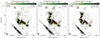 |
Fig. 5. Polarization intensity maps (5″ resolution) at VLA L-, S-, and C-band after performing RM-synthesis. Red lines represent the magnetic field vectors. Their orientation represents the projected B-field corrected for Faraday rotation and contribution from the Galactic foreground. The vector lengths are proportional to the polarization percentage and their lengths are corrected for Ricean bias. No vectors were drawn for pixels below 5σ in the polarized intensity image. The distinct filaments, namely F1 and F2 (for labeling see Fig. 1), and some regions embedded in the halo emission are polarized between 10–38% between 1 and 6.5 GHz. At all the observed frequencies, the B-field across the relic and other features is highly-ordered. Contour levels are drawn at |
![Mathematical equation: $ \sqrt{[1,2,4,8,\dots]}\,\times\,5\,\sigma_{\mathrm{{ rms}}} $](/articles/aa/full_html/2022/01/aa42340-21/aa42340-21-eq7.gif)
At 5″, the polarization fraction across the relic varies from about 2%, which is the lowest value for a detection of polarized emission in our maps, up to about 40% between 1 and 5.5 GHz. In Table 2, we also report the average fractional polarization measured from 5″ maps in the relic subregions. These values are consistent with those reported by Bonafede et al. (2009) but are lower than measured from our 2″ resolution maps. This implies that the degree of polarization increases with increasing resolution, mainly by a factor of about 1.4 (for a resolution improving by a factor of 2.5). At low resolution, regions with different polarization characteristics become blurred within a single resolution element, leading to a loss of the observed polarized signal. This effect is known as beam depolarization and it is expected to be lower if the source is imaged at a higher resolution. In Fig. 5, we also show a clear and sharp distinction between the main relic and the filaments (F1 and F2), apparently protruding from the relic.
As shown in Figs. 3 and 5, the average fractional polarization across the relic increases from R1 to R3 also in L-band and S-band. Moreover, the southern part of the relic is still significantly polarized in L-band. In contrast, the northern part of the relic seems to be depolarized from the C-band to L-band.
In Fig. 6, we show depolarization maps of the relic at 2″ and 5″ resolutions. The depolarization fraction is defined as DP = p1.5 GHz/p5.5 GHz, where p1.5 GHz and p5.5 GHz are the fractional polarization values at 1.5 GHz and 5.5 GHz, respectively. As evident, for the northern part of the relic, we find strong depolarization (DP < 0.4) between 1.5 GHz and 5.5 GHz. In particular, the R1 region of the relic is almost fully depolarized at 1.5 GHz. For the southern part, the depolarization fraction (DP > 0.6) is less significant, compared to the northern part. There is also clear beam depolarization when comparing the 2″ and 5″ resolution maps; see Table 2 for the average depolarization fraction values across the subregions of the relic.
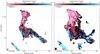 |
Fig. 6. Depolarization maps of the relic between 1.5 and 5.5 GHz at 2″ (left) and 5″ (right) angular resolution. The depolarization fraction is defined as DP = p1.5 GHz/p5.5 GHz. DP = 0 implies full depolarization while DP = 1 means no depolarization. These maps demonstrate that the northern part of the relic is strongly depolarized, in particular the R1 region of the relic. |
5. Faraday rotation analysis
The polarization properties of diffuse sources in clusters are vital for understanding their origin and formation scenarios. Moreover, they may serve as a powerful tool to disentangle the contribution from different emission regions that are otherwise blended along the line of sight in the continuum emission.
One of the most important physical effects to consider when discussing radio polarimetric observations is Faraday rotation. It occurs when a radio wave on its way to the observer passes through a magnetoionic medium which causes the polarization angle, ψobs, to vary as a function of the wavelength (λ). The strength of the Faraday effect is measured by the rotation measure (RM):
 (4)
(4)
We note that we use RM to exclusively indicate how rapidly the polarization angle changes with λ2. In observations, the polarization angle is obtained from the Stokes parameters Q and U of linearly polarized emission via:
 (5)
(5)
A magnetoionic medium causes a rotation of the polarization angle according to
 (6)
(6)
The difference in Faraday depth (Δϕ) is given by integrating a section of the light traveling path (Δl)
 (7)
(7)
where the thermal electron density (ne), the magnetic field component along the line of sight (B∥), and the path length (l) are in units of cm−3, μG, and pc, respectively. The Faraday depth denotes the integral given in Eq. (7) when the path length is taken from the observer to an arbitrary point along the line of sight. If there is only one source of emission along the line of sight, the Faraday depth of the source position equals the RM obtained from the polarization analysis. If the emission has a more complex distribution in Faraday depth, the derivative in Eq. (4) does not allow us to draw any conclusion on the Faraday depth distribution in a simple, straightforward way.
Polarization studies of extragalactic sources have shown that a significant number of extended radio sources cannot be described by a single component in terms of Faraday depth (e.g., O’Sullivan et al. 2012; Anderson et al. 2015). Hence, the angle of Faraday rotation for multiple rotating or emitting screens along the line of sight is characterized by a distribution of Faraday depths (ϕ) instead of a single component. For a mixed Faraday-rotating and synchrotron-emitting medium, the observed polarized intensity may originate from a broad range of Faraday depths.
The RM, as given in Eq. (4), determined in the observers frame, would differ from similar measurements carried out closer to the source, for example, in the rest-frame of the source, since the photons get redshifted from the source to the observer due to the cosmological expansion (Kim et al. 2016; Basu et al. 2018). Specifically, if in the rest-frame of the source, located at redshift zRM, a RM of RMint is determined, the cosmological expansion would lead, in the observers frame, to an RM of
 (8)
(8)
if no magnetoionic medium is present along the line of sight.
Analyzing the Faraday rotation is a powerful method by which to investigate extragalactic magnetic fields. Observations of the polarization angle as a function of frequency may provide crucial information about the magnetization of the source and of the medium intervening along the line of sight.
What is fundamental to this analysis is carrying out a measurement of the polarization angle over a wide range of wavelengths. As discussed above, the polarization angle may depend in a complex way on wavelength if there is polarized emission with a wide spread of Faraday depths along the line of sight (Burn 1966; Tribble 1991; Sokoloff et al. 1998). Faraday rotation may originate inside the radio emitting region if enough thermal gas is mixed with the synchrotron radiating plasma (internal Faraday dispersion). Alternatively, it could be of external origin if magnetized thermal gas is present along the line of sight (external Faraday dispersion).
The VLA L-, S-, and C-band data allow us to carry out a detailed wideband polarization study of the compact and diffuse radio sources in MACS J0717.5+3745. We used two methods to infer the Faraday distribution: a rotation measure synthesis (RM-synthesis) and QU-fitting.
5.1. RM-synthesis
The RM-synthesis technique, developed by Brentjens & de Bruyn (2005), is based on the theoretical description of Burn (1966).
The intensity of linearly polarized emission and its polarization angle ψ can be expressed as a complex number
 (9)
(9)
where I is the total intensity of the source and p0 is the fraction of polarized emission. Following Burn (1966), the wavelength dependent polarization, P(λ2), can be written as a Fourier transform
 (10)
(10)
where ϕ is the Faraday depth which here became an independent variable, forming the Faraday space. F(ϕ) is known as the Faraday dispersion function (FDF) and describes the amount of polarized emission originating from a certain Faraday depth. F(ϕ) can be measured as
 (11)
(11)
The RM-synthesis calculates F(ϕ) by the Fourier transformation of the observed polarization as a function of wavelength-squared. The rotation measure spread function (RMSF), which is analogous to the synthesized image beam, describes the instrumental response to the polarized signal in Faraday space. We refer to Brentjens & de Bruyn (2005) for details of this technique.
The RMSF is determined by the total coverage in λ2-space of the observations. Since the finite frequency band produces a broad RMSF with sidelobes, deconvolution is advantageous. We used the deconvolution algorithm RM CLEAN (Heald 2009) for this purpose.
The RM-synthesis was carried out using the pyrmsynth1 code. We performed RM-Synthesis on the Stokes Q and U cubes at two different resolutions, namely, 4″ and 12.5″. The 4″ resolution cube was used to study the relic region while the low resolution 12.5″ to study the low-surface-brightness polarized emission features that are not detected at high resolution. The RM-synthesis cube synthesized a range of Faraday depths from −800 rad m−2 to +800 rad m−2, with a bin size of 2 rad m−2. We used the entire L-, S-, and C-band data. These data give a sensitivity to the polarized emission up to a resolution in Faraday depth (δϕ) equal to
 (12)
(12)
where Δλ2 =  . The high Faraday-space resolution may allow us to separate multiple, narrowly spaced, Faraday-space components. We also ran pyrmsynth individually only on the L-, S-, and C-band data. The resulting polarization intensity images for L-, S-, and C-band, overlaid with the total intensity contours, are shown in Fig. 5.
A more detailed study of the Faraday distribution of the relic in MACS J0717.5+3745 is not available in the literature. Bonafede et al. (2009) did perform a simple linear fit to the polarization angle as a function of λ2 and found poor agreement between the data and the linear ansatz. In the left panel of Fig. 7, we show the high-resolution Faraday depth map of the relic. The map represents, for each pixel (sky coordinate), the Faraday depth ϕmax at which the FDF has its maximum. At the position of MACS J0717.5+3745, the average Galactic RM contribution is +16 rad m−2 (Oppermann et al. 2012). This value is also consistent with the RM that we observe for the southern foreground galaxy, ϕFRI = +16 ± 0.1 rad m−2.
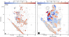 |
Fig. 7. Faraday depth (ϕmax) maps of the relic in MACS J0717.5+3745 measured over 1.0–6.5 GHz using RM-synthesis technique. Left: high-resolution (4″) Faraday map. The ϕmax distribution across the relic, in particular in the northern part is patchy with coherence lengths of 10–50 kpc. Right: low-resolution (12.5″) Faraday depth map. The measured ϕmax values in the polarized halo region are similar to the R3 region of the relic, indicating very little Faraday rotation intervening material. This suggests that these regions are located on the near side of the cluster. |
For the relic, the peak Faraday depth (ϕmax) values vary across the relic between −30 to +40 rad m−2. The peak Faraday depth distribution tends to be patchy with patch sizes of about 10-50 kpc. For the southern part of the relic, the observed peak Faraday depth ranges mainly from +7 to +25 rad m−2. Stronger variations in the peak Faraday depth are visible for the northern part of the relic, in particular, the R1 region.
To further investigate the Faraday distribution in the relic, we use 64 square-shaped regions with an edge length of 5″ covering the entire relic. These regions are shown in the left panel of Fig. 4. Each region defines a “box” in the Faraday cube when taking the Faraday depth axis into account. For each box, we obtained a FDF (see Fig. 8 for examples). We find that the FDF of most of the boxes is dominated by a pronounced single component, except for a few (e.g., boxes 4, 5, and 34).
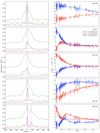 |
Fig. 8. Comparison between RM-synthesis and QU-fitting for boxes 49, 4, 10, 24, and 34. Left: cleaned (black) and dirty (green) Faraday dispersion functions (FDF) obtained using RM-synthesis. The red dashed line is drawn at the 8σQU level. The magenta lines indicate the peak positions (ϕmax) of the FDFs. Right: corresponding QU-fitting spectra, the fractional Stokes q (blue) and q (red) with the dots showing the QU-spectra measured in the boxes and the dashed and solid lines are the one and two component fits, respectively. We also mark the one and two component fits with brown circles and dark blue asterisks to clearly indicate the significance of these markers used in subsequent images. For boxes 4, 10, 24, and 34, the QU-spectra are better fitted with two components. Correspondingly, RM-synthesis shows broader FDF for these boxes. For simple regions, the example box 49 is shown. We find that both RM-synthesis and QU-fitting appears to be consistent with a single Faraday component. |
For the southern part of the relic (boxes 33–64), the peak Faraday depth in the boxes is well defined and relatively uniform (e.g., see panel a of Fig. 8). The analysis confirms that the southern part of the relic shows a peak Faraday depth very close to the Galactic foreground, implying very little Faraday rotating material intervening along the line of sight to the emission region in the cluster.
For the northern part of the relic (boxes 1–32), in particular for the R1 region, the analysis reveals strong peak Faraday depth variations, with no particular coherent structure. As seen in the left panel of Fig. 8, the Faraday dispersion functions extracted across the northern part of the relic tend to be broader and less symmetric than those extracted from the southern part. The broader FDFs hint to the presence of emission at different Faraday depths. There are two basic scenarios leading to a complex FDF: either the emission is extended along the line of sight embedded in a magnetoionic medium or there is a magnetoionic medium with a complex Faraday depth distribution in front of the emission. Of course, there can also be mixture of both.
5.2. QU-fitting
An alternative approach to interpreting broadband polarimetric data is to approximate the observed quantities Q(λ2) and U(λ2), referred to here as “QU-spectra” hereafter, over the broad wavelength range using an analytic model with a small number of free parameters. We refer to this method as “QU-fitting”. This technique is particularly powerful when the FDF is rather simple and can be described by an analytic model which can be guessed, for example, from the geometry of the source, the most likely morphology of the magnetic field, or knowledge about the medium intervening along the line of sight to the source (e.g., Farnsworth et al. 2011; Ozawa et al. 2015; Anderson et al. 2015, 2016, 2018; Pasetto et al. 2018).
The polarized signal from the boxes introduced in the previous section is well suited for this approach: According to the generally accepted scenario for the origin of radio relics, electrons are accelerated at cluster-sized merger shocks and radiate in a comparably thin layer downstream of the shock. In the sky area covered by one box, we expect to see only a small part of the merger shock front. The width of each box corresponds to a physical size of 32 kpc. If the line of sight to a box intersects the shock front only once and the front is inclined to the line of sight, the emission received from the box area originates from a volume that is rather small, as compared to the cluster dimensions. It is only if the shock front is seen very close to edge-on, the volume will be significantly extended along the line of sight. Based on this scenario, we expect that the Faraday distribution in each box is reasonably well described by a single component in Faraday space. The ICM and the intergalactic medium (IGM), intersecting the line-of-sight to the emission volume, determine the position of the component in Faraday space and its width, with the latter manifested by the depolarization of the emission.
We assume, that the complex polarization P of a single Gaussian component in Faraday space can be expressed via:
 (13)
(13)
where I(λ2) is the total intensity as a function of λ2, p the intrinsic polarization fraction, ϕc the average Faraday depth of the emission (i.e., the position of the center of the Gaussian component) and σϕ the Faraday dispersion (i.e., the width of the Gaussian component). In a more general model, also the intrinsic polarization fraction and intrinsic polarization angle ψ could be wavelength-dependent. We emphasize that the single Gaussian component ansatz is based on the scenario that we observe in each box only a small emission volume with a screen in front of it showing a Gaussian Faraday depth distribution. A more complex distribution of the emission or a non-Gaussian Faraday depth distribution of the screen would require a more complex description. Based on the motivation detailed above, we expect the model to provide a good approximation to the data.
To eliminate any spectral effects, we use the fractional properties q = Re(P)/I and u = Im(P)/I. The “one Gaussian component” model functions become:
 (14a)
(14a)
 (14b)
(14b)
We approximate the QU-spectra in three steps as follows: (i) First, we scan the four-dimensional parameter space (p, ψ, ϕc, σϕ) and compute the difference between model and data χ2 for each set of parameters. The difference is computed according to
 (15)
(15)
where λi denotes the central wavelength of the spectral channel i, x the two fractional properties q and u, and σx, i the uncertainty of the measurement for  and
and  in the boxes; (ii) Starting from the parameter set with the lowest χ2, we run a Levenberg-Marquardt parameter optimization; (iii) Starting from the optimized parameter set, we finally run a Markov chain Monte Carlo (MCMC).
In the right panel of Fig. 8, we show the QU-fitting results for boxes 49, 4, 10, 24, and 34. The top panel, box 49, shows the QU-spectra of a region from the southern part of the relic, namely the R3 region. As evident, the one-component model provides a very good fit. For the other boxes shown in Fig. 8, we find that there are systematic differences between the data and model, indicating that the actual Faraday distribution is more complex than the one Gaussian component ansatz.
In Fig. 9, we show the residuals after subtracting the best one-component fit for the boxes 4, 10, 24, and 34. The systematic differences between the measured QU-spectra and the fits are evident. As an ad-hoc model, we assume that the actual Faraday distribution can be better fitted by two Gaussian components in Faraday space. We therefore approximate the QU-spectra with the sum of two independent one-component models. To determine the model parameters, we follow the steps as given above but using eight independent parameters.
 |
Fig. 9. Residual QU-spectra for the boxes 4, 10, 24, and 34 obtained after subtracting the best one component fit. The blue and red circles show the observed fractional q minus the best one component fit (q1c) and the observed fractional u minus the best one component fit (u1c), respectively. The systematic differences between the QU-spectra measured in the boxes and the fits are evident. |
Figure 10 (upper panel) shows the resulting reduced χ2 for each box fitted with one and then two Gaussian components. For some regions, the one component model (brown circles) already results in a reduced value of χ2 that is close to one, suggesting that the data are reasonably well approximated. We note that the reduced χ2 = 1 is only achieved for a perfect match between data and model if the uncertainties of the data reflect the uncertainty of independent measurements. It is beyond the scope of this work to study in detail if the Stokes IQU data are indeed fully independent. Therefore, even a perfectly matched model may show a reduced χ2 slightly deviating from one. Some boxes show a reduced χ2 much larger than one, for example, boxes 4, 7, and 35, indicating a poor fit. As expected, the two Gaussian component model (dark blue asterisks in Fig. 10) better matches the data, generally resulting in a lower reduced χ2. However, we adopt only the two-component model with the significantly larger number of free parameters if the fit is substantially better. We therefore employ the Bayesian information criterion (BIC):
 (16)
(16)
 |
Fig. 10. Results from QU-fitting. The best-fit parameters obtained by fitting a single and two independent one-component models are shown. The one component model fits are indicated with brown filled circles and the two component models with dark blue and cyan asterisks. The resulting reduced χ2 for each box is shown in the top panel and the BIC in the second one. If the BIC of the two component fit lower than the one component fit, the former is adopted for further analysis. For theses boxes the best fit parameters are shown with cyan and dark blue asterisks where the cyan color is assigned to the component with the higher Faraday dispersion. The third, fourth, and fifth panels show the intrinsic polarized luminosity, Sν, pol, the Faraday dispersion, and the position for each of the Gaussian components. Finally, the Boxes used for extracting the Stokes IQU values are shown Fig 4. The plot shows that many regions in R1 and R2 are fitted better using two components. |
where N denotes the number of independent data points and Nvar the number of free parameters in the fit. Figure 10 second row shows the BIC for the one (BICOC) and the two Gaussian component (BICTC) model for all boxes. For about half of the boxes, the BIC of the two component model is lower (large symbols in Fig. 10) indicating a substantially better fit. We note that for some boxes, for example boxes 31 and 53, the reduced χ2 is lower for the two components, the BIC, in contrast is higher for the two components. Since the decision is based on the BIC, we adopt in these cases the one component model for further analysis, underlining that the BIC requires a significantly better fit for adopting two components for the further analysis.
In Fig. 10, we also show the model polarized flux density at 4 GHz (third row) for all boxes, the Faraday dispersion obtained for each box (fourth row), and the central Faraday depth of the Gaussian components (fifth row). Based on the BIC, we adopt the two Gaussian component model only if it fits the data substantially better.
5.3. RM-synthesis versus QU-fitting
The QU-fitting has revealed that for most of the boxes a single Gaussian component provides a reasonable approximation, even if for about half of the boxes provide an even better approximation. Since we used two methods, namely, QU-fitting and RM-synthesis, to determine the Faraday structure of the emission in the boxes, it is interesting to compare the results of the two methods. Since the one-component fit provides a reasonable fit (i.e., the reduced χ2 does not differ very much from one; see Fig. 10 first panel) we do expect to obtain from the RM-synthesis method a single peak for most of the boxes as well.
Since the RM-synthesis shows a single peak for most of the boxes, we do expect that the peak in the FDF does correspond to the central Faraday depth of a single Gaussian component fit. We note that we use here for simplicity the single component fit for all boxes. The peak Faraday depth from RM-synthesis is read from the uncleaned (dirty) spectra. Figure 11 shows a reasonable agreement between the peak ϕmax and the central Faraday depth. Apparently, broad differences occur only for boxes with a very broad single component, that is, where the Faraday dispersion σϕ is large and the emission is depolarized at longer wavelengths. For instance, box 4 shows a ϕc of +43 rad m−2 and a ϕmax of +14 rad m−2, the Faraday dispersion of a single component fit in the box is 56 rad m−2.
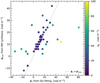 |
Fig. 11. Central Faraday depth, ϕc, position of the single component from QU-fitting (see Fig. 10 brown markers. We note that here we use the one-component fit for all boxes) versus peak position, ϕmax in the RM-synthesis spectra. The color indicates the Faraday depth width of the QU-fitting component. Evidently, QU-fitting and RM-synthesis gives similar results in case of a low Faraday dispersion. Larger differences between QU-fitting and RM-synthesis correspond to higher Faraday dispersions. |
Evidently, the Faraday dispersions σϕ of many single component fits are very small. For instance, σϕ in the boxes 47, 48, and 49 is about 18 rad m−2 in observers frame. RM-synthesis does not allow us to clearly recover such small Faraday dispersions, that is widths of FDFs, even after RM cleaning (see Fig. 8 box 49). For box 34, from the QU-fitting the two-component version is preferred, showing one component at 20 rad m−2 and one at 165 rad m−2. It is interesting to note that the central Faraday depth position of the two components agrees well with the two peaks found in RM-synthesis, see Fig. 8.
We conclude that (i) in situations with one single dominating component and weak depolarization, the peak Faraday depth from RM-synthesis and the central Faraday depth from QU-fitting agree well; (ii) in situations of strong depolarization, the results may differ significantly; and (iii) two clearly separated components in Faraday space can be recovered by both methods. However, we would like to emphasize that for RM-synthesis no assumptions are made for FDF, so much more general distributions might be found that allow us to reproduce the QU-spectra. We also note that RM-synthesis is sometimes reported to fail to find the underlying Faraday distribution for even the simple case of two components (Farnsworth et al. 2011; O’Sullivan et al. 2012).
6. Faraday distribution of the relic
In Fig. 12, we show the central Faraday depth and Faraday dispersion maps for the southern part of the relic obtained from QU-fitting. For the relic regions R3 and R4, QU-fitting and RM-synthesis (see Fig. 7) consistently reveal a rather uniform distribution of the central Faraday depth, which apparently reflects the Galactic foreground of +16 rad m−2 (Oppermann et al. 2012). Except in the NAT regions, almost all boxes are well fitted with one component according to the BIC (see Fig. 10). In this part of the relic, the Faraday dispersion values are in the range of ∼ 10−20 rad m−2 (at the redshift of the observer). The depolarization in these boxes corresponds to a mean Faraday dispersion of about σϕ ∼ 12 rad m−2 in the observer’s frame. The Faraday dispersion likely reflect intrinsic depolarization in the relic (internal depolarization) or Faraday depth variations caused by the ICM intervening along the line of sight to the relic (external depolarization). In both scenarios, the source for depolarization is in the cluster, hence, we have to take into account the redshift effect discussed above (see Eq. (8)). The mean Faraday dispersion at the location of the cluster amounts to σϕ,R3+R4 ∼ 29 rad m−2. Interestingly, the Sausage relic shows a similar Faraday dispersion (Di Gennaro et al. 2021).
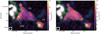 |
Fig. 12. ϕc and σϕ values across the R3 and R4 region of the relic obtained with QU-fitting. For almost all boxes the one Gaussian component model is preferred, except for the region where the NAT galaxy is located. We note that for the NAT region only the low dispersion component is shown in the figure, matching the ϕc of the relic. Moreover, the left panel (red lines) shows the intrinsic polarization angle. The QU-fitting results are overlaid on the polarization intensity at 5″ and contours of the VLA L-band Stokes I image; see Table 1, IM6 for the image properties. Contour levels are drawn at [1, 2, 4, 8, …] × 5 σrms. From these maps, it is evident that ϕc and σϕ are low in this region of the relic, particularly in the R3 region and not changing significantly from box to box. The central Faraday depth of the Gaussian components are very close to the Galactic foreground RM, indicating very little Faraday rotation due material intervening the line of sight to cluster outside of the Milky Way. This suggests that this part of the relic is located at the periphery of the cluster towards the observer. |
The central Faraday depth and Faraday dispersion maps for the northern part of the relic are shown in Fig. 13. RM-synthesis and QU-fitting reveal complex Faraday depth and dispersion distributions. The scatter of the central Faraday depth increases from south to north. This is consistent with the pixel-wise Faraday depth peak position analysis as shown in Fig. 7 obtained from RM-synthesis. Moreover, in this region of the relic, the Faraday dispersion values vary up to 170 rad m−2. As can be seen from Fig. 13, lower panels, σϕ systematically increases from south to north, that is, from box 32 to box 1 (see also Fig. 10).
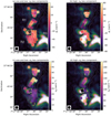 |
Fig. 13. Central Faraday depth and Faraday dispersion values for the northern part of the relic obtained with QU-fitting. Top: ϕc values for one component and low Faraday dispersion components (panel a) and the high Faraday dispersion two components (panel b). For a large number of regions, we find the presence of two Faraday components; the one component or the low Faraday dispersion component in case of two components (left panels) and the high Faraday dispersion components (right panels). Bottom: σϕ values for one component and low Faraday dispersion components (panel c) and the high Faraday dispersion two components (panel d). The majority of the polarized emission is at rather high σϕ, suggesting that the northern part of the relic is located in or behind the ICM. Contours and image properties are as in Fig. 12. |
From the parameters of R1, that is all boxes up to box 13, as shown in Fig. 10, we compute the average Faraday dispersion (σϕ) of all components. Weighting the parameters according to their uncertainty, we find an average of 47 rad m−2, that is 114 rad m−2 at the redshift of the cluster. Interestingly, the standard variation of the central Faraday depth is lower, namely 39 rad m−2, that is 93 m−2 at the redshift of the cluster. The uncertainties of the parameters has again been used as weights. The fact that the average dispersion is a factor of 1.22 lower than the scatter of positions in Faraday space may indicate that the magnetic field along the line of sight shows significant fluctuations on scales of the size of the boxes (i.e., 32 kpc) or smaller.
In Fig. 14, we show the Faraday dispersion versus central Faraday depth for all boxes and all components. The plot shows again that the scatter of the central Faraday depth increases with increasing Faraday dispersion. The offset central Faraday depth due to the Galactic foreground of +16 rad m−2 is evident. The dashed lines indicate σϕ = ±1.22 · (ϕc − 16 rad m−2), where the factor 1.22 is used according to the discussion above. The results in Fig. 14 corroborate that the standard deviation of the central Faraday depth of the components obtained for the boxes is lower than the Faraday dispersion obtained from the depolarization.
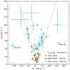 |
Fig. 14. Central Faraday depth as a function of Faraday dispersion, measured in the observer’s frame. Dashed lines indicate σϕ = 1.22(ϕc − 16 rad m−2), where 16 rad m−2 is the Faraday depth due to the Galactic foreground. One component models are indicated with brown filled circles and two component models with black and cyan stars, where black indicates the component with the lower Faraday dispersion and cyan the higher one. Components shown in Fig. 10 with a very large uncertainties are neglected here because they do not provide any constraint. The plot shows that the scatter of the central Faraday depth increases with increasing Faraday dispersion. |
The correlation between the scatter of the central Faraday depth and the Faraday dispersion is consistent with and gives evidence for the scenario that the emission with a higher Faraday depth is located deeper in the cluster or has a larger amount of ICM in front of it which causes the Faraday rotation. Interestingly, the parameters obtained for both components of the two component fit follow the correlation. Retaining the scenario that a slab of ICM in front of the emission causes both the central Faraday depth and the Faraday dispersion, this could be interpreted as two different patches of ICM in front of a single emission found in one box; alternatively, there could be two different emission regions along the line of sight within one box.
The high-resolution total power images (left and middle panels of Fig. 15) and spectral tomography analysis (right panel of Fig. 15) have revealed that the northern part of the relic is composed of multiple filaments (van Weeren et al. 2017b; Rajpurohit et al. 2021c). These filaments are denoted with red arrows in Fig. 15. In these regions, there is a component that is almost always at or near the mean Galactic Faraday depth with a low Faraday dispersion while the second component shows much larger scatter in Faraday depth and a high value of Faraday dispersion. It could be that these features are part of the same shock front, located either in or behind the cluster, but there is also some emission closer to the observer. If true, the presence of two Faraday components may suggest that these filaments may be separated in Faraday space along the line of sight and we see them in projection. The second component, therefore, indicates two emission regions significantly separated along the line of sight. It is also worth noting that the intrinsic polarizations in the two components apparently show rather similar intrinsic polarization angles. This could be considered as an argument in favor of the “two patches of ICM in front of single emission” scenario.
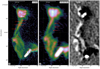 |
Fig. 15. High-resolution VLA (left panel; van Weeren et al. 2017b) and uGMRT (middle panel; Rajpurohit et al. 2020a) images of the northern part of the relic. The red arrows show regions with fine filaments. The spectral tomography map of the same region is shown in the right panel, indicating that the relic is indeed composed of filaments with different spectral indices (Rajpurohit et al. 2021c). For the majority of these regions, the QU-fitting provides a better fit with two Faraday components. |
In general, the Faraday distribution of the relic seems to be consistent with a tangled magnetic field in the ICM which is in front of the emission. It is beyond the scope of this work to draw conclusions based on the correlation of the scatter of the central Faraday depth and the Faraday dispersion on the possible magnetic field distribution in the ICM. However, it is interesting to note that the ratio between dispersion and scatter is about 1.22. This may indicate that there is power on scales of the size of box or smaller in the power spectrum of the magnetic field distribution.
The second component in boxes 33 and 34 shows a very low and very high central Faraday depth, respectively, that is clearly outside the correlation found for the other components. The two boxes contain emission from the NAT, as discussed in more detail in Sect. 8. It is therefore plausible to assume that the Faraday depth of these two components is not solely caused by the ICM.
Detailed Faraday rotation studies, over a sufficient frequency range, have been performed so far only for eight radio relics, namely, for Abell 2256 (Owen et al. 2014; Ozawa et al. 2015), the Coma relic (Bonafede et al. 2013), Abell 2255 (Govoni et al. 2005; Pizzo et al. 2011), RXC J1314.4-2515 (Stuardi et al. 2019), CIZA J2242.8+5301 (aka the “Sausage relic”; Kierdorf et al. 2017; Loi et al. 2017; Di Gennaro et al. 2021), Abell 2345 (Stuardi et al. 2021), Abell 2744 (Rajpurohit et al. 2021b), and 1RXS J0603.3+4214 (aka “Toothbrush relic”; van Weeren et al. 2012; Kierdorf et al. 2017). In these relics, the Faraday rotation has been reported to be mainly caused by Galactic foreground, with no strong evidence for frequency-dependent depolarization, for example, the Sausage relic (Kierdorf et al. 2017; Di Gennaro et al. 2021). In addition, the Faraday dispersion is mainly found to be below 40 rad m−2.
To the best of our knowledge, it is only for parts of the Toothbrush and Abell 2256 relics that the observed RMs deviate from the Galactic foreground and show significantly high Faraday dispersion values (van Weeren et al. 2012; Kierdorf et al. 2017; Ozawa et al. 2015). Recently, we studied the Toothbrush relic at 18.6 GHz and found a strong depolarization between 4.9 and 18.5 GHz, corresponding to a Faraday rotation measure dispersion of 212±23 rad m−2 (Rajpurohit et al. 2020b). The relic in MACS J0717.5+3745 is the first relic clearly showing a high σϕ derived on the basis of a spatially well-resolved analysis. For example, a median Faraday dispersion in R1 of 114 rad m−2 in the rest-frame of the cluster. Such a high value of σϕ implies that the ICM magnetic field is highly tangled even on scales as small as a few tens of kpc.
7. Intrinsic polarization angle at the shock
The orientation of the observed polarization vectors provides valuable clues to the nature of diffuse emission. Merger-shock models predict the relic should be highly polarized only when viewed close to edge-on (Skillman et al. 2013). For the Sausage and the Toothbrush relics, which are very likely seen edge-on, high polarization fractions (55%–70%) have been reported (van Weeren et al. 2010, 2012; Loi et al. 2020; Rajpurohit et al. 2020b; Di Gennaro et al. 2021). It is believed that the high polarization fraction in relics is due to shock waves, which compress and hence align isotropically distributed magnetic fields. For the relic in MACS J0717.5+3745, the polarization fraction reaches about 30% or more in some regions. Such a degree of polarization rules out the possibility that the relic is seen face-on.
In Fig. 5, we show the magnetic field (B-field) orientation distribution at L-, S-, and C-bands. The lines represent the plane of polarization (E-field) rotated by 90° to better visualize the magnetic field structure. We find that the B-field orientations are aligned across the relic at all three frequencies. This implies that the magnetic field orientation is well correlated along the entire extent of the relic and is mostly aligned with the shock front. The distribution of magnetic field orientations in the MACS J0717.5+3745 relic is very similar to what is found for the Sausage relic (van Weeren et al. 2010; Di Gennaro et al. 2021).
The magnetic field orientation distribution (intrinsic) obtained from QU-fitting is shown in Figs. 12 and 13; these are effectively corrected for the local and Galactic Faraday rotation. It is evident that the field orientations are aligned with the source extension for both single and two independent RM components. We note that for many boxes with two components, the polarization angle is approximately the same for both components. Recently, using advanced simulations Domínguez-Fernández et al. (2021) found that intrinsic polarization angles (E-vectors) in relics strongly depend on the upstream properties of the medium and find that a turbulent medium can result in a highly aligned (anisotropic) magnetic field distribution at the shock front. The field orientation distribution in the MACS J0717.5+3745 is consistent with that simulation.
To resolve some fine structures, a high spatial resolution (2″) vector map is shown in Fig. 16. Even at full resolution, we still do not find any small-scale deviation of the magnetic field orientation from the source morphology.
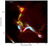 |
Fig. 16. Faraday-corrected magnetic field (B-field) orientation (pink lines) of the relic overlaid on the 2″ resolution total intensity (red), S-band polarization (green), and L-band polarization (blue) images. The image demonstrates well aligned B-field vectors with the orientation of emission. This suggests a high degree of ordering of the B-field across the entire relic. The image properties are given in Table 1, IM5 and IM9. |
In the polarization images, R3 appears to be connected with R2 by a region of low-surface-brightness emission (see the middle panel of Fig. 2 and 5). The change in the orientation of the B-field between the northern and southern part of the relic and this low-surface-brightness emission connecting them is evident. The observed gradual change in B-field orientation and the RM gradient from R1 to R4 hints that the northern and southern parts of the relic are part of the same physical structure rather than two independent sources seemingly aligned in projection. This point is further discussed in Sect. 10.
8. Connection between the NAT and the relic
At the location of the NAT, (in particular for boxes 33-36), we find that a one-component Faraday screen provides a very poor fit to the QU-spectra while the two-component model instead allows us to fit q and u reasonably well. These regions cover the NAT core and the tails (about 94 kpc distance from the core). We note that the tails of the NAT are even more extended at frequencies below 700 MHz and they bend toward the south of R3. However, the bent tails are barely visible above 1.5 GHz (Rajpurohit et al. 2021c).
We find that boxes 33–36 and 41–43, as well as 45, coinciding with the NAT, show a clear second component with a high Faraday dispersion compared to the relic R3 region. The central Faraday depth of the high Faraday dispersion component varies significantly from box to box (see Fig. 10), as expected from a Faraday screen with a tangled magnetic field. Therefore, it is plausible to assume that the Faraday dispersion of about 150 rad m−2 (at the redshift of the cluster), which indicates that these components have a significantly thicker ICM in front of them than the relic in that region. However, for boxes 33 and 34, we find that the second component falls outside the relation between Faraday dispersion and scatter of the central Faraday depth that is typically found for almost all components. This might be explained by part of the Faraday depth that is found for these components being intrinsic to the emission and not caused by the ICM in front of it. Therefore, it is also conceivable that part of the Faraday dispersion has to be attributed to be intrinsic to the NAT and is not caused by the ICM in front of the emission. Therefore, any interpretation of the Faraday structure of these components has to be taken with some grains of salt.
A plausible scenario for the structure and polarization properties of the NAT galaxy is that the galaxy is actually deep in the cluster or even at the rear side of the cluster. Evidently, the head-tail morphology indicates the interaction with the ICM. The Faraday dispersion of these components suggests a similar amount of magnetized ICM in front of the NAT than in front of many components of R1 and R2 and clearly a larger amount than in front of R3 and R4.
In the total power images, the emission located within box 44 appears to be connected to R3 through a bright, thin filamentary structure; see the region shown with cyan in Fig. 15 right panel. Box 44 is significantly polarized (∼30%), with a typically low value of σϕ (13 rad m−2). The low σϕ suggests less path length through the ICM: that is the emission must be lying in the cluster periphery towards the observer. The high degree of polarization indicates, rather, that the contribution of the NAT is likely to be faint. We do not find any evidence that the NAT is moving diagonally through the cluster where the R3 region of the relic is located. If this were the case in boxes 33, 34, 35, 36, 37, and 44, we would expect to see a component from a region with high σϕ propagating towards a region with a lower σϕ. We do not find any hint of such a component.
Our analysis supports a scenario in which the NAT is moving through the cluster, coming from the observer, and is deep in the cluster causing the high σϕ. In contrast to the NAT, R3 shows a polarized emission component with low σϕ, indicating very little Faraday rotating intervening material, implying that the relic is located in front of the ICM or in the cluster periphery. This suggests that the NAT and R3 are well separated in Faraday space and, thus not connected physically. The spectral analysis of the same region also revealed two spectral components (Rajpurohit et al. 2021c).
On the basis of the polarization and spectral analysis, we suggest that the NAT and R3 overlap only in the projection, whereas in the cluster, they are, in fact, separated. This makes it unlikely that the NAT can be the source of seed electrons that are re-accelerated by the shock front at the relic.
9. Viewing angle of the merger
Based on the theoretical model by Ensslin et al. (1998), it is possible to estimate the orientation of the merger axis using the average degree of polarization (e.g., Hoang et al. 2018). Here, we use the approximation for weak magnetic fields (Eq. (3.2) in Ensslin et al. 1998) to estimate the viewing angle of the relic in MACS J0717.5+3745. We estimated the viewing angle for the four regions of the relic: R1, R2, R3, and R4. Our results are given in Fig. 17. The three black curves give the theoretical estimate of the average polarization fraction depending on the viewing angle for spectral indices of −1.18, −1.17, −1.16, and −1.13 of the four subregions (see Table 2). The theoretical predictions for the four indices do not differ significantly.
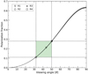 |
Fig. 17. Viewing angle versus polarization fraction relation for the MACS J0717.5+3745 relic. A viewing angle of 90° implies that the merger is in the plane of the sky (i.e., perpendicular to the shock). The four solid curves, that are nearly identical, give the theoretical predictions for spectral indices of α = −1.18, −1.13, −1.17, and −1.16, for the relic subregions. The triangle, circle, star, and square provide the corresponding estimates for the relic subregions R1, R2, R3, and R4. The dashed lines indicate the minimum and maximum value of the mean polarization fraction and the viewing angle. The possible viewing angles of MACS J0717.5+3745 fall inside the green shaded region. The plot shows that the relic in MACS J0717.5+3745 is seen to be less edge-on. |
We use the average intrinsic polarization fractions measured for the four subregions from QU-fitting (see the symbols in Fig. 17). We found that the regions R2 and R4 are seen at an angle of 50.1° to 50.3°, while R1 and R4 appear to be seen at angles of 43.8° and 32°, respectively. Radio relics are not straight sheet-like structures, but have rather complex 3D-shapes (e.g., Skillman et al. 2013; Wittor et al. 2017, 2019; Dominguez-Fernandez et al. 2021). Hence, it is very likely that different parts of the relic are seen under different viewing angles. The radio emission from relics are not spherically symmetric and thus their morphology depends on the viewing angle of the radio emission. The fact that the different regions of the MACS J0717.5+3745 relic are seen at such different viewing angles could well explain its chair-like structure.
The average intrinsic polarization fraction (obtained from QU-fitting) implies that the relic in MACS J0717.5+3745 is seen less edge-on compared to some other relics, for instance, the Sausage (van Weeren et al. 2010; Kierdorf et al. 2017; Loi et al. 2020; Di Gennaro et al. 2021) and Toothbrush (van Weeren et al. 2012; Kierdorf et al. 2017; Rajpurohit et al. 2020b) relics, which show a rather high degree of polarization and are most likely seen edge-on. We note that the intrinsic polarization could be an underestimation because fractional polarization may still suffer from beam depolarization. The viewing angle of the MACS J0717.5+3745 relic is in the range 32° ≤θ ≤ 51°, this is also consistent with the one obtained from the radio color-color analysis (Rajpurohit et al. 2021c).
10. Comparison with simulations
We compare the polarization properties of the MACS J0717.5+3745 relic with the simulated relic from Wittor et al. (2019). As discussed above, the viewing angle of the relic is at least 45° (i.e., the viewing angle of the merger is 45° with respect to the plane of the sky). Therefore, in the following section, we compare the polarization properties of the simulated relic when seen at 45° to that of the MACS J0717.5+3745 relic.
We carried out the simulation with the cosmological magneto-hydrodynamical ENZO code (Bryan et al. 2014). It belongs to a sample of high-resolution simulations of galaxy clusters that was used to study magnetic field properties in the ICM (Vazza et al. 2018; Domínguez-Fernández et al. 2019). These simulations self-consistently evolve complex magnetic field patterns during cluster mergers, starting from an assumed uniform “primordial” seed field, with 0.1 of the seed comoving nG at z = 40. The model for producing synthetic radio observations is explained in detail in Wittor et al. (2019). In brief, the model accounts for the acceleration of a tiny fraction of electrons from the thermal pool (based on the thermal leakage model) via DSA at the shock front, as well as for the aging of cosmic-ray electrons in the downstream region of the shock front. As the simulated relic was found to mimic several spectral properties of the MACS J0717.5+3745 relic, here we investigate RM fluctuations and gas perturbations in the shock front region.
Figure 18 shows the RM distribution of the simulated relic. In the simulation, we study two different scenarios for the location of the relic with respect to the observer: the relic either in front or behind the cluster (see insets in the RM maps in Fig. 18). If the relic lies behind the cluster, the X-ray emission provides a good proxy for the amount of ICM the radio emission has to transverse. In Fig. 18, we plot the maps of the average RM along the line of sight of the simulated relic. The RM maps are weighted with the radio power at 1.4 GHz and, hence, they are meant to reflect the RM measured at the brightest region of the relic along the line of sight.
 |
Fig. 18. Simulations presented as maps of the average RM, radio weighted at 1.4 GHz. Left: RM distribution if the relic lies in front of the cluster, as depicted in the inset. Right: RM distribution if the relic lies behind the cluster, as show in the inset. These maps show that strong fluctuations in the RM are expected if the relic is located within, or behind, the ICM screen. |
If the relic lies in front of the cluster, the resulting RM values are similar to the southern part of the relic in MACS J0717.5+3745, except for a larger value close to the dense sub-clump in the region (see Fig. 1 of Wittor et al. 2019). On the other hand, if the relic is located behind the cluster, the RM values in the simulations are similar to the ones measured for the relic in MACS J0717.5+3745. These larger RM values are attributed to the fact that the simulated relic lies deeper inside the ICM. Furthermore, the simulated relic shows an RM trend when moving from north to south (see Fig. 18). The relative decrease is also similar to the observed decrease from region R1 to R4 in the MACS J0717.5+3745 relic. Such a gradient is missing if the relic is in front of the cluster.
If the relic is instead located behind the cluster, the RM increases from the north of the relic to the south. The reason for this behavior is twofold. First, the top part is located in a less dense ICM. Second, the relic is tilted with respect to the line of sight and, hence, the top part lies closer to the observer. Therefore, such an RM trend is expected if a part of the relic is located in or behind a denser ICM, or at a larger distance from the observer as a denser ICM can boost the strength of the RM gradient.
Similar trends in RM are observed for the relic in MACS J0717.5+3745: the northern part of the relic in MACS J0717.5+3745 is located in or behind the dense ICM, whereas the southern part extends into the low density ICM; see discussion in Sect. 6. We emphasize that the simulated relic is a single structure caused by the same shock front. This raises an important question regarding whether R1+R2 and R3+R4 are a connected structure that is simply inclined (or tilted) towards the line of sight or whether they belong to two different structures that appear to be connected in projection. If part of the relic is at a larger distance to the observer, the emitting structure is either disconnected or tilted with respect to the line of sight. The latter seems to be a more likely explanation for the relic in MACS J0717.5+3745 (see discussion in Sect. 7); however the current data do not allow us to rule out the possibility that the northern and southern parts are disconnected.
11. Magnetic field estimates
The combination of observed Faraday dispersion and central Faraday depth trends across the relic can be used to constrain the magnetic field properties of the ICM. Both the strength and the morphology of magnetic fields affect the Faraday depth of radio sources. Under a few simplifying assumptions, we can use the observed Faraday dispersion (σϕ) to estimate the magnetic field values following, for example, Sokoloff et al. (1998), Kierdorf et al. (2017):
 (17)
(17)
where ⟨ne⟩ is the average thermal electron density of the ionized gas along the line of sight in cm−3, Bturb is the magnetic field strength in μG, and f the volume filling factor of the Faraday-rotating plasma. L and t are the path length through the thermal gas and turbulence scale, respectively, in pc.
For the relic in MACS J0717.5+3745, we find fluctuations in the polarization intensity on a scale as small as 10 kpc (see Sect. 4), particularly for the northern part of the relic. This may hint that the turbulence coherence length is of the same scale. Therefore, we adopt t = 10 kpc. We assume that the path which is dominating the Faraday depth scatter is where the density is highest along the path (i.e., L) and has a length of 1 Mpc. Depending on the line of sight and density, this could be close to the cluster center with high density or rather in the periphery. We consider the thermal electron density of ⟨ne⟩ = 10−3 cm−3. Finally, the filling factor is assumed to be 0.5 following Murgia et al. (2004), Kierdorf et al. (2017)
A significant number of boxes in R1 and R2 regions provide a better fit with two Faraday components, however, for the magnetic field estimate, we only considered the low Faraday dispersion component. For the northern part of the relic, the mean σϕ of the low Faraday dispersion component is about 120 rad m−2 (in the rest-frame of the cluster). By inserting all values in Eq. (17), we obtained Bturb, R1+R2 ∼ 1.8 μG. When using ⟨ne⟩ = 10−4 cm−3, we get a very high value of magnetic field (∼ 18 μG), which is unlikely because in this case, we would expect much higher value of σϕ.
For the southern part of the relic, the mean Faraday dispersion is about 29 rad m−2 (in the rest-frame of the cluster). We note that the region contaminated by the NAT is excluded. Since the σϕ is low compared to the northern part of the relic and also the fluctuations in the polarization intensity, we assume ⟨ne⟩ = 10−4 cm−3, L = 1.5 Mpc and t = 100 kpc. For this part of the relic, we obtained Bturb, R3+R4 ∼ 1.2 μG.
If the estimated strength of the turbulent magnetic field and the turbulent scale reflects the properties of the ICM, this suggests that the northern component of the relic is embedded in a moderately dense ICM. Since the Faraday dispersion and the magnetic field are not very high (at least for the low Faraday dispersion component), it is very unlikely that this part of the relic is located behind the ICM. On the other hand, the southern part favors a geometry in which the line of sight passes through a region of the ICM that is slightly less dense or passes in front of the ICM.
12. Possible polarization of the halo emission
The halo in MACS J0717.5+3745 exhibits a significant substructure (e.g., van Weeren et al. 2017b). It remains uncertain whether or not those filamentary substructures can be entirely attributed to the halo (tracing regions of increased turbulence) or whether they are similar to relics (tracing shock waves). We note that the estimated viewing angle suggests that some structures might indeed be only seen in projections with the halo.
Polarized emission from radio halos has been very difficult to detect. Cluster-wide polarized emission from halos has not yet been detected from any cluster. So far, polarized filamentary structures have been detected only in three halos, namely. MACS J0717.5+3745, Abell 2255, and Abell 523 (Govoni et al. 2005; Bonafede et al. 2009; Girardi et al. 2016). However, in these three cases, it is still not clear that the polarized emission is truly associated with the halos. The absence of polarization in halos has been interpreted as the result of internal Faraday rotation and beam depolarization. The low surface brightness also limits the possibility of detecting the polarized signal from a radio halo. The halo in MACS J0717.5+3745 is one of the most powerful known halos; since the measured surface brightness is typically higher in powerful halos, this cluster offers one of the best opportunities to detect any polarized emission that may be present (Govoni et al. 2013).
Bonafede et al. (2009) reported polarized emission from the radio halo associated with MACS J0717.5+3745, with a mean fractional polarization of 5% at 1.4 GHz from a 20″ resolution image. However, it is not yet fully clear whether this polarized emission truly comes from the halo emission, or rather from the relic emission projected along the line of sight.
The high-resolution polarization intensity images reveal only a few patches of polarized emission in the halo region (see Figs. 3 and 5). Since radio halos typically have a low surface brightness and are often not detected in high resolution images, we also created moderate-resolution (12.5″) polarized intensity images. In Fig. 19, we show these moderate-resolution polarized intensity maps at L-, S-, and C-bands. At this resolution, we are much more sensitive to low-surface-brightness emission.
 |
Fig. 19. Low-resolution (12.5″ resolution) polarization intensity overlaid with the total intensity contours, showing that a part of the halo is polarized (shown with green arrows). Contour levels are drawn at |
![Mathematical equation: $ \sqrt{[1,2,4,8,\dots]}\,\times\,4\,\sigma_{\mathrm{{ rms}}} $](/articles/aa/full_html/2022/01/aa42340-21/aa42340-21-eq26.gif)
As shown in Fig. 19, we detect more polarized emission in the halo region in our low-resolution images. This indicates that the magnetic field is very likely not tangled on scales smaller than the beam size in these regions. We detect patches of polarized emission from the halo (indicated with green arrows). We note that the regions of the halo with filamentary substructures, visible in Stokes I, are polarized with a fractional polarization of 8–36%. Excluding these polarized patches, the polarized halo emission is below the 1σ level.
To calculate an upper limit on the fractional polarization of the halo, we used our moderate-resolution polarization image at 3 GHz. We exclude polarized regions that are shock related and projected on the halo, as mentioned above. For the 12.5″ resolution polarized intensity image at 3 GHz, the σQ, U is 9 μJy beam−1 RMSF−1. We found no polarized emission at greater than 5σQ, U within the region of the radio halo. From the Stokes I image, we find a peak halo flux density of 1.9 μJy beam−1 at 3 GHz. Therefore, our 5σQ, U upper limit on the fractional polarization for the halo at 3 GHz is 3%. It is important to emphasize here that these polarization images were obtained using deep observations (45 hours on-source VLA observations combining A, B, C, and D configurations) with high sensitivity to low-surface-brightness emission.
The polarized intensity map (see Fig. 19) clearly shows a discontinuity between the polarized structures in the halo region and the relic. In addition, there also exists a clear separation between the polarized emission detected in the halo emission and filaments F1 and F2. The low-resolution Faraday map is shown in the right panel of Fig. 7. The Faraday map shows a uniform distribution across the halo region with a mean Faraday depth of +18 rad m−2. The σϕ in these regions is of the order of 11−16 rad m−2. If this polarized emission were from a halo, we would expect high values of σϕ with significant fluctuations arising from the dense ICM; we do not find any evidence of such behavior. The observed Faraday depth values are consistent with being Galactic in origin, which suggests that the emission is not experiencing significant Faraday rotation from the ICM. We also find similar Faraday depth values for filaments F1 and F2. Moreover, at least F1 is apparently located in the cluster outskirt. Towards the cluster center, the radio emission experiences greater Faraday rotation, thus we expect a high value of Faraday dispersion value. The low σϕ values found for polarized patches in the halo region suggest that these regions are in fact located toward the cluster outskirts.
The filamentary substructures, including F1 and F2, found in the halo region are significantly polarized. We find that the magnetic field vectors are highly ordered in these polarized regions, typical for shock-related structures; see Fig. 5. In addition, F1 shows a distinct behavior in the point-to-point radio versus X-ray surface-brightness relation (Rajpurohit et al. 2021a), suggesting the emission in F1 is not associated with the halo and has a different origin. Considering all the evidence presented in this section, we suggest that these polarized filaments are shock-related structures projected onto the cluster center and the halo region.
13. Summary and conclusions
In this work, we present VLA L-, S-, and C-band polarimetric radio observations of the galaxy cluster MACS J0717.5+3745. Thanks to the very wide bandwidth of the combined observations and the high angular resolution of the images, it has been possible to reveal the complexity of diffuse radio emission in polarized intensity. Polarization and Faraday depth maps, with resolution ranging from 2″ to 12.5″, along with QU-spectra in 64 regions were constructed and analyzed to study the origin of the diffuse emission in the cluster. We summarize the overall results as follows:
-
The relic is highly polarized with a polarization fraction > 30% in some regions. Between 2–6.5 GHz, polarized emission is detected along the whole extent of the relic. The polarized emission is clumpier than the total power emission. The fractional polarization changes systematically; increases from R1 to R3.
-
By comparing rotation measure (RM) synthesis and QU-fitting results, we find a reasonable agreement when the Faraday dispersion functions are simple and the depolarization is low or modest.
-
A strong wavelength-dependent Faraday depolarization is detected between 1 GHz and 6.5 GHz for the northern part of the relic (R1 and R2). The underlying Faraday dispersion may originate from an intervening magnetized screen that arises from dense ICM containing a tangled magnetic field. The high depolarization of the northern part of the relic, corresponding to a Faraday dispersion (σϕ) of about 30−170 rad m−2 (in the observer-frame) suggests that the northern part of the relic is located in or behind the ICM.
-
For the southern part of the relic (R3 and R4), we find a single Faraday component and a low value of σϕ (below 20 rad m−2, in the observer-frame). The Faraday depth (ϕc) values are very close to the Galactic foreground, indicating very little Faraday-rotating material along the line of sight toward this part of the relic. This suggests that the southern part of the relic is likely to reside in a lower-density region of the ICM or is located in the front of the cluster.
-
For a number of subregions (“boxes”) in the relic regions R1 and R2, we find that the QU-spectra are significantly better modeled when two Gaussian Faraday components are adopted instead of one. The second component exhibits rather high σϕ (as high as ∼ 170 rad m−2, in the observer-frame). We find strong spatial variation in both ϕc and σϕ. These fluctuations are consistent with a magnetic field in the ICM that is tangled on a scale of a few tens of kpc.
-
From spatially resolved analysis, we find that the scatter of Faraday depth is correlated with depolarization, corroborating the notion that a tangled field in the ICM is the cause of depolarization.
-
The magnetic field orientations derived from the polarization angle are well-aligned along the relic structure. This indicates that the magnetic field distribution in the plane of the sky within the relic is highly anisotropic, which is very likely due to compression as a result of the passage of the merger shock wave.
-
We find evidence of two clear Faraday components along the line of sight that are passing through the NAT galaxy. The presence of two Faraday components indicates that there is also a relic component at that location. We suggest that the NAT and the R3 region of the relic are separated in Faraday space, such that the NAT is either located in or behind the ICM while the relic component (associated with R3) lies in front of the ICM. If true, this implies that the relic is not seeded by the shock re-acceleration of fossil electrons from the NAT galaxy.
-
The degree of polarization across filaments F1 and F2 is > 15%. We find generally low Faraday depth values across both of these structures, confirming that they are located in the cluster outskirts. The magnetic field in these structures is well ordered, as typical for relics. Therefore, these filaments are very likely shock-related structures.
-
We detect polarized emission from filamentary structures found within the halo region from both high- and low-resolution VLA maps. The absence of significant Faraday rotation, the aligned magnetic field orientations within the emitting region and the generally low σϕ suggests that these polarized emission features, previously considered to be part of the halo, are related to shocks projected onto the cluster center and the halo region.
-
We do not detect any significant polarized emission truly associated with the halo in our deep (45 hours on-source time) and highly sensitive VLA observations. The upper limit on the fractional polarization for the halo at 3 GHz is 3%.
The spatially resolved polarization and Faraday analysis of the complex merging galaxy cluster MACS J0717.5+3745 suggests that the ICM magnetic field is highly tangled. The observed depolarization and high value of Faraday dispersion are consistent with an intervening magnetized screen that arises from the dense ICM. Based on the spectral and polarization properties, we conclude that several of the observed properties of this system are dominated by a superposition of plasma mediums containing tangled fields along the line of sight.
Acknowledgments
M. H. thanks A. Basu for enlightening discussions. K. R., F. V., M. Brienza, and N. L. acknowledge financial support from the ERC Starting Grant “MAGCOW”, no. 714196. M. H. and A. D. acknowledge financial support by the BMBF with the grant number 05A20STA. D. W. acknowledges financial support by the Deutsche Forschungsgemeinschaft (DFG, German Research Foundation) – 441694982. RJvW and A. Botteon acknowledge support from the VIDI research programme with project number 639.042.729, which is financed by the Netherlands Organization for Scientific Research (NWO). L. R. acknowledges support, in part from US National Science Foundation grant AST 17-14205 to the University of Minnesota. W. Forman acknowledges support from the Smithsonian Institution, the High Resolution Camera Project through NASA contract NAS8-03060, and NASA Grants 80NSSC19K0116, GO1-22132X, and GO9-20109X. C. J. R., E. B., M. Brienza, and A. Bonafede acknowledge support from the ERC through the grant ERC-Stg DRANOEL n. 714245. P. D. F. acknowledges support by the National Research Foundation (NRF) of Korea through grants 2016R1A5A1013277 and 2020R1A2C2102800. F. L. acknowledges financial support from the Italian Minister for Research and Education (MIUR), project FARE, project code R16PR59747, project name FORNAX-B. A part of the data reduction was performed using computer facilities at Thüringer Landessternwarte Tautenburg, Germany. This research made use of computer facility on the HPC resources at the Physical Research Laboratory (PRL), India. The cosmological simulations in this work were performed using the ENZO code (http://enzo-project.org). The authors gratefully acknowledge the Gauss Centre for Supercomputing e.V. (www.gauss-centre.eu) for supporting this project by providing computing time through the John von Neumann Institute for Computing (NIC) on the GCS Supercomputer JUWELS at Jülich Supercomputing Centre (JSC), under projects no. HHH42 and stressicm (PI F.Vazza) as well as HHH44 (PI D. Wittor). We also acknowledge the usage of online storage tools kindly provided by the INAF Astronomical Archive (IA2) initiave (http://www.ia2.inaf.it). The National Radio Astronomy Observatory is a facility of the National Science Foundation operated under cooperative agreement by Associated Universities. Finally, we wish to acknowledge the developers of the following python packages, which were used extensively during this project: aplpy (Robitaille & Bressert 2012), astropy (Astropy Collaboration 2013), matplotlib (Hunter 2007), numpy (van der Walt et al. 2011) and scipy (Jones et al. 2001).
References
- Anderson, C. S., Gaensler, B. M., Feain, I. J., & Franzen, T. M. O. 2015, ApJ, 815, 49 [Google Scholar]
- Anderson, C. S., Gaensler, B. M., & Feain, I. J. 2016, ApJ, 825, 59 [NASA ADS] [CrossRef] [Google Scholar]
- Anderson, C. S., Gaensler, B. M., Heald, G. H., et al. 2018, ApJ, 855, 41 [NASA ADS] [CrossRef] [Google Scholar]
- Astropy Collaboration (Robitaille, T. P., et al.) 2013, A&A, 558, A33 [NASA ADS] [CrossRef] [EDP Sciences] [Google Scholar]
- Basu, A., Mao, S. A., Fletcher, A., et al. 2018, MNRAS, 477, 2528 [NASA ADS] [CrossRef] [Google Scholar]
- Beck, R. 2015, A&ARv, 24, 4 [Google Scholar]
- Blandford, R., & Eichler, D. 1987, Phys. Rep., 154, 1 [Google Scholar]
- Bonafede, A., Feretti, L., Giovannini, G., et al. 2009, A&A, 503, 707 [NASA ADS] [CrossRef] [EDP Sciences] [Google Scholar]
- Bonafede, A., Vazza, F., Brüggen, M., et al. 2013, MNRAS, 433, 3208 [NASA ADS] [CrossRef] [Google Scholar]
- Bonafede, A., Intema, H. T., Brüggen, M., et al. 2014, ApJ, 785, 1 [Google Scholar]
- Bonafede, A., Brüggen, M., Rafferty, D., et al. 2018, MNRAS, 478, 2927 [Google Scholar]
- Botteon, A., Gastaldello, F., Brunetti, G., & Kale, R. 2016, MNRAS, 463, 1534 [Google Scholar]
- Botteon, A., Gastaldello, F., & Brunetti, G. 2018, MNRAS, 476, 5591 [Google Scholar]
- Botteon, A., Brunetti, G., Ryu, D., & Roh, S. 2020, A&A, 634, A64 [NASA ADS] [CrossRef] [EDP Sciences] [Google Scholar]
- Brentjens, M. A., & de Bruyn, A. G. 2005, A&A, 441, 1217 [NASA ADS] [CrossRef] [EDP Sciences] [Google Scholar]
- Briggs, D. S. 1995, Am. Astron. Soc. Meeting Abstr., 187, 112.02 [NASA ADS] [Google Scholar]
- Brunetti, G., & Jones, T. W. 2014, Int. J. Mod. Phys. D, 23, 1430007 [Google Scholar]
- Brunetti, G., Setti, G., Feretti, L., & Giovannini, G. 2001, MNRAS, 320, 365 [Google Scholar]
- Bryan, G. L., Norman, M. L., O’Shea, B. W., et al. 2014, ApJS, 211, 19 [Google Scholar]
- Burn, B. J. 1966, MNRAS, 133, 67 [Google Scholar]
- Carilli, C. L., & Taylor, G. B. 2002, ARA&A, 40, 319 [NASA ADS] [CrossRef] [Google Scholar]
- Di Gennaro, G., van Weeren, R. J., Hoeft, M., et al. 2018, ApJ, 865, 24 [Google Scholar]
- Di Gennaro, G., van Weeren, R. J., Rudnick, L., et al. 2021, ApJ, 911, 3 [NASA ADS] [CrossRef] [Google Scholar]
- Domínguez-Fernández, P., Vazza, F., Brüggen, M., & Brunetti, G. 2019, MNRAS, 486, 623 [Google Scholar]
- Dominguez-Fernandez, P., Bruggen, M., Vazza, F., et al. 2021, MNRAS, 500, 795 [Google Scholar]
- Domínguez-Fernández, P., Brüggen, M., Vazza, F., et al. 2021, MNRAS, 507, 2714 [Google Scholar]
- Donnert, J., Vazza, F., Brüggen, M., & ZuHone, J. 2018, Space Sci. Rev., 214, 122 [Google Scholar]
- Drury, L. O. 1983, Rep. Prog. Phys., 46, 973 [Google Scholar]
- Ensslin, T. A., Biermann, P. L., Klein, U., & Kohle, S. 1998, A&A, 332, 395 [NASA ADS] [Google Scholar]
- Farnsworth, D., Rudnick, L., & Brown, S. 2011, AJ, 141, 191 [NASA ADS] [CrossRef] [Google Scholar]
- George, S. J., Stil, J. M., & Keller, B. W. 2012, PASA, 29, 214 [Google Scholar]
- Girardi, M., Boschin, W., Gastaldello, F., et al. 2016, MNRAS, 456, 2829 [CrossRef] [Google Scholar]
- Govoni, F., & Feretti, L. 2004, Int. J. Mod. Phys. D, 13, 1549 [Google Scholar]
- Govoni, F., Murgia, M., Feretti, L., et al. 2005, A&A, 430, L5 [NASA ADS] [CrossRef] [EDP Sciences] [Google Scholar]
- Govoni, F., Murgia, M., Xu, H., et al. 2013, A&A, 554, A102 [NASA ADS] [CrossRef] [EDP Sciences] [Google Scholar]
- Heald, G. 2009, IAU Symp., 259, 591 [Google Scholar]
- Hoang, D. N., Shimwell, T. W., van Weeren, R. J., et al. 2018, MNRAS, 478, 2218 [Google Scholar]
- Hoeft, M., & Brüggen, M. 2007, MNRAS, 375, 77 [Google Scholar]
- Hunter, J. D. 2007, Comput. Sci. Eng., 9, 90 [NASA ADS] [CrossRef] [Google Scholar]
- Johnson, A. R., Rudnick, L., Jones, T. W., Mendygral, P. J., & Dolag, K. 2020, ApJ, 888, 101 [Google Scholar]
- Jones, E., Oliphant, T., Peterson, P., et al. 2001, SciPy: Open source scientific tools for Python, [Online; accessed - today] [Google Scholar]
- Kang, H., & Ryu, D. 2011, ApJ, 734, 18 [Google Scholar]
- Kierdorf, M., Beck, R., Hoeft, M., et al. 2017, A&A, 600, A18 [NASA ADS] [CrossRef] [EDP Sciences] [Google Scholar]
- Kim, K. S., Lilly, S. J., Miniati, F., et al. 2016, ApJ, 829, 133 [NASA ADS] [CrossRef] [Google Scholar]
- Klein, U., & Fletcher, A. 2015, Galactic and Intergalactic Magnetic Fields [Google Scholar]
- Laing, R. A. 1980, MNRAS, 193, 439 [NASA ADS] [Google Scholar]
- Loi, F., Murgia, M., Govoni, F., et al. 2017, MNRAS, 472, 3605 [NASA ADS] [CrossRef] [Google Scholar]
- Loi, F., Murgia, M., Vacca, V., et al. 2020, MNRAS, 498, 1628 [NASA ADS] [CrossRef] [Google Scholar]
- Mohan, N., & Rafferty, D. 2015, PyBDSM: Python Blob Detection and Source Measurement (Astrophysics Source Code Library) [Google Scholar]
- Murgia, M., Govoni, F., Feretti, L., et al. 2004, A&A, 424, 429 [NASA ADS] [CrossRef] [EDP Sciences] [Google Scholar]
- Ogrean, G. A., Brüggen, M., van Weeren, R. J., et al. 2013, MNRAS, 433, 812 [Google Scholar]
- Oppermann, N., Junklewitz, H., Robbers, G., et al. 2012, A&A, 542, A93 [NASA ADS] [CrossRef] [EDP Sciences] [Google Scholar]
- O’Sullivan, S. P., Brown, S., Robishaw, T., et al. 2012, MNRAS, 421, 3300 [CrossRef] [Google Scholar]
- Owen, F. N., Rudnick, L., Eilek, J., et al. 2014, ApJ, 794, 24 [Google Scholar]
- Ozawa, T., Nakanishi, H., Akahori, T., et al. 2015, PASJ, 67, 110 [NASA ADS] [CrossRef] [Google Scholar]
- Pandey-Pommier, M., Richard, J., Combes, F., et al. 2013, A&A, 557, A117 [NASA ADS] [CrossRef] [EDP Sciences] [Google Scholar]
- Pasetto, A., Carrasco-González, C., O’Sullivan, S., et al. 2018, A&A, 613, A74 [NASA ADS] [CrossRef] [EDP Sciences] [Google Scholar]
- Pearce, C. J. J., van Weeren, R. J., Andrade-Santos, F., et al. 2017, ApJ, 845, 81 [Google Scholar]
- Perley, R. A., & Butler, B. J. 2013, ApJS, 204, 19 [Google Scholar]
- Petrosian, V. 2001, ApJ, 557, 560 [Google Scholar]
- Pizzo, R. F., de Bruyn, A. G., Bernardi, G., & Brentjens, M. A. 2011, A&A, 525, A104 [NASA ADS] [CrossRef] [EDP Sciences] [Google Scholar]
- Rajpurohit, K., Hoeft, M., van Weeren, R. J., et al. 2018, ApJ, 852, 65 [Google Scholar]
- Rajpurohit, K., Hoeft, M., Vazza, F., et al. 2020a, A&A, 636, A30 [NASA ADS] [CrossRef] [EDP Sciences] [Google Scholar]
- Rajpurohit, K., Vazza, F., Hoeft, M., et al. 2020b, A&A, 642, L13 [EDP Sciences] [Google Scholar]
- Rajpurohit, K., Brunetti, G., Bonafede, A., et al. 2021a, A&A, 646, A135 [NASA ADS] [CrossRef] [EDP Sciences] [Google Scholar]
- Rajpurohit, K., Vazza, F., van Weeren, R. J., et al. 2021b, A&A, 654, A41 [NASA ADS] [CrossRef] [EDP Sciences] [Google Scholar]
- Rajpurohit, K., Wittor, D., van Weeren, R. J., et al. 2021c, A&A, 646, A56 [EDP Sciences] [Google Scholar]
- Robitaille, T., & Bressert, E. 2012, APLpy: Astronomical Plotting Library in Python (Astrophysics Source Code Library) [Google Scholar]
- Sarazin, C. L., Finoguenov, A., & Wik, D. R. 2013, Astron. Nachr., 334, 346 [NASA ADS] [Google Scholar]
- Skillman, S. W., Xu, H., Hallman, E. J., et al. 2013, ApJ, 765, 21 [Google Scholar]
- Sokoloff, D. D., Bykov, A. A., Shukurov, A., et al. 1998, MNRAS, 299, 189 [Google Scholar]
- Stuardi, C., Bonafede, A., Wittor, D., et al. 2019, MNRAS, 489, 3905 [NASA ADS] [Google Scholar]
- Stuardi, C., Bonafede, A., Lovisari, L., et al. 2021, MNRAS, 502, 2518 [NASA ADS] [CrossRef] [Google Scholar]
- Tribble, P. C. 1991, MNRAS, 250, 726 [NASA ADS] [CrossRef] [Google Scholar]
- van der Walt, S., Colbert, S. C., & Varoquaux, G. 2011, Comput. Sci. Eng., 13, 22 [Google Scholar]
- van Weeren, R. J., Röttgering, H. J. A., Brüggen, M., & Cohen, A. 2009, A&A, 505, 991 [NASA ADS] [CrossRef] [EDP Sciences] [Google Scholar]
- van Weeren, R. J., Röttgering, H. J. A., Brüggen, M., & Hoeft, M. 2010, Science, 330, 347 [Google Scholar]
- van Weeren, R. J., Röttgering, H. J. A., Intema, H. T., et al. 2012, A&A, 546, A124 [NASA ADS] [CrossRef] [EDP Sciences] [Google Scholar]
- van Weeren, R. J., Brunetti, G., Brüggen, M., et al. 2016a, ApJ, 818, 204 [Google Scholar]
- van Weeren, R. J., Ogrean, G. A., Jones, C., et al. 2016b, ApJ, 817, 98 [Google Scholar]
- van Weeren, R. J., Ogrean, G. A., Jones, C., et al. 2017a, ApJ, 835, 197 [Google Scholar]
- van Weeren, R. J., Andrade-Santos, F., Dawson, W. A., et al. 2017b, Nat. Astron., 1, 0005 [Google Scholar]
- van Weeren, R. J., de Gasperin, F., Akamatsu, H., et al. 2019, Space Sci. Rev., 215, 16 [Google Scholar]
- Vazza, F., Brunetti, G., Brüggen, M., & Bonafede, A. 2018, MNRAS, 474, 1672 [NASA ADS] [CrossRef] [Google Scholar]
- Wardle, J. F. C., & Kronberg, P. P. 1974, ApJ, 194, 249 [Google Scholar]
- Wittor, D., Vazza, F., & Brüggen, M. 2017, MNRAS, 464, 4448 [NASA ADS] [CrossRef] [Google Scholar]
- Wittor, D., Hoeft, M., Vazza, F., Brüggen, M., & Domínguez-Fernández, P. 2019, MNRAS, 490, 3987 [Google Scholar]
- Wittor, D., Vazza, F., Ryu, D., & Kang, H. 2020, MNRAS, 495, L112 [NASA ADS] [CrossRef] [Google Scholar]
All Tables
Polarization properties of the diffuse radio emission in the cluster MACS J0717.5+3745.
All Figures
|
Fig. 1. Composite total power, polarization intensity, and X-ray image of the relic in MACS J0717+3745 at 2″ resolution. The total power and L-band polarization emission are shown in red and green-yellow, respectively. The intensity in blue shows the X-ray emission. The lack of polarized emission in the north region (R1) indicates depolarization. The image properties are given in Table 1, IM5 and IM9. |
| In the text | |
|
Fig. 2. Polarization intensity images of the relic in MACS J0717.5+3745 at 2″ resolution, showing that the polarization emission is distributed in a clumpy manner. The image also revels fine, small-scale filaments visible in the total power emission. Contour levels are drawn at |
| In the text | |
|
Fig. 3. High-resolution (2″) fractional polarization maps at VLA L-, S-, and C-bands. The relic is polarized at all of the observed frequencies, reaching values up to 50% in some regions. The northern part of the relic strongly depolarizes at 1.5 GHz. Contour levels are drawn at |
| In the text | |
|
Fig. 4. Left: VLA L-band image depicting regions used for flux density extraction and RM-synthesis and QU-fitting. Blue regions show the relic subregions where the average fractional polarization was extracted. The fractional polarization at R3 in Table 2 is obtained by excluding the contribution from the NAT. Red boxes where flux densities and Faraday dispersion functions were extracted for QU-fitting and RM-synthesis, respectively. Each red box has a width of 5″, corresponding to a physical size of 32 kpc. Right: fractional polarization profiles across the relic extracted from the rectangular regions, depicted in the inset, of width 2″. There is a hint that the fractional polarization decreases in the downstream regions (i.e., shown with arrows). |
| In the text | |
|
Fig. 5. Polarization intensity maps (5″ resolution) at VLA L-, S-, and C-band after performing RM-synthesis. Red lines represent the magnetic field vectors. Their orientation represents the projected B-field corrected for Faraday rotation and contribution from the Galactic foreground. The vector lengths are proportional to the polarization percentage and their lengths are corrected for Ricean bias. No vectors were drawn for pixels below 5σ in the polarized intensity image. The distinct filaments, namely F1 and F2 (for labeling see Fig. 1), and some regions embedded in the halo emission are polarized between 10–38% between 1 and 6.5 GHz. At all the observed frequencies, the B-field across the relic and other features is highly-ordered. Contour levels are drawn at |
| In the text | |
|
Fig. 6. Depolarization maps of the relic between 1.5 and 5.5 GHz at 2″ (left) and 5″ (right) angular resolution. The depolarization fraction is defined as DP = p1.5 GHz/p5.5 GHz. DP = 0 implies full depolarization while DP = 1 means no depolarization. These maps demonstrate that the northern part of the relic is strongly depolarized, in particular the R1 region of the relic. |
| In the text | |
|
Fig. 7. Faraday depth (ϕmax) maps of the relic in MACS J0717.5+3745 measured over 1.0–6.5 GHz using RM-synthesis technique. Left: high-resolution (4″) Faraday map. The ϕmax distribution across the relic, in particular in the northern part is patchy with coherence lengths of 10–50 kpc. Right: low-resolution (12.5″) Faraday depth map. The measured ϕmax values in the polarized halo region are similar to the R3 region of the relic, indicating very little Faraday rotation intervening material. This suggests that these regions are located on the near side of the cluster. |
| In the text | |
|
Fig. 8. Comparison between RM-synthesis and QU-fitting for boxes 49, 4, 10, 24, and 34. Left: cleaned (black) and dirty (green) Faraday dispersion functions (FDF) obtained using RM-synthesis. The red dashed line is drawn at the 8σQU level. The magenta lines indicate the peak positions (ϕmax) of the FDFs. Right: corresponding QU-fitting spectra, the fractional Stokes q (blue) and q (red) with the dots showing the QU-spectra measured in the boxes and the dashed and solid lines are the one and two component fits, respectively. We also mark the one and two component fits with brown circles and dark blue asterisks to clearly indicate the significance of these markers used in subsequent images. For boxes 4, 10, 24, and 34, the QU-spectra are better fitted with two components. Correspondingly, RM-synthesis shows broader FDF for these boxes. For simple regions, the example box 49 is shown. We find that both RM-synthesis and QU-fitting appears to be consistent with a single Faraday component. |
| In the text | |
|
Fig. 9. Residual QU-spectra for the boxes 4, 10, 24, and 34 obtained after subtracting the best one component fit. The blue and red circles show the observed fractional q minus the best one component fit (q1c) and the observed fractional u minus the best one component fit (u1c), respectively. The systematic differences between the QU-spectra measured in the boxes and the fits are evident. |
| In the text | |
|
Fig. 10. Results from QU-fitting. The best-fit parameters obtained by fitting a single and two independent one-component models are shown. The one component model fits are indicated with brown filled circles and the two component models with dark blue and cyan asterisks. The resulting reduced χ2 for each box is shown in the top panel and the BIC in the second one. If the BIC of the two component fit lower than the one component fit, the former is adopted for further analysis. For theses boxes the best fit parameters are shown with cyan and dark blue asterisks where the cyan color is assigned to the component with the higher Faraday dispersion. The third, fourth, and fifth panels show the intrinsic polarized luminosity, Sν, pol, the Faraday dispersion, and the position for each of the Gaussian components. Finally, the Boxes used for extracting the Stokes IQU values are shown Fig 4. The plot shows that many regions in R1 and R2 are fitted better using two components. |
| In the text | |
|
Fig. 11. Central Faraday depth, ϕc, position of the single component from QU-fitting (see Fig. 10 brown markers. We note that here we use the one-component fit for all boxes) versus peak position, ϕmax in the RM-synthesis spectra. The color indicates the Faraday depth width of the QU-fitting component. Evidently, QU-fitting and RM-synthesis gives similar results in case of a low Faraday dispersion. Larger differences between QU-fitting and RM-synthesis correspond to higher Faraday dispersions. |
| In the text | |
|
Fig. 12. ϕc and σϕ values across the R3 and R4 region of the relic obtained with QU-fitting. For almost all boxes the one Gaussian component model is preferred, except for the region where the NAT galaxy is located. We note that for the NAT region only the low dispersion component is shown in the figure, matching the ϕc of the relic. Moreover, the left panel (red lines) shows the intrinsic polarization angle. The QU-fitting results are overlaid on the polarization intensity at 5″ and contours of the VLA L-band Stokes I image; see Table 1, IM6 for the image properties. Contour levels are drawn at [1, 2, 4, 8, …] × 5 σrms. From these maps, it is evident that ϕc and σϕ are low in this region of the relic, particularly in the R3 region and not changing significantly from box to box. The central Faraday depth of the Gaussian components are very close to the Galactic foreground RM, indicating very little Faraday rotation due material intervening the line of sight to cluster outside of the Milky Way. This suggests that this part of the relic is located at the periphery of the cluster towards the observer. |
| In the text | |
|
Fig. 13. Central Faraday depth and Faraday dispersion values for the northern part of the relic obtained with QU-fitting. Top: ϕc values for one component and low Faraday dispersion components (panel a) and the high Faraday dispersion two components (panel b). For a large number of regions, we find the presence of two Faraday components; the one component or the low Faraday dispersion component in case of two components (left panels) and the high Faraday dispersion components (right panels). Bottom: σϕ values for one component and low Faraday dispersion components (panel c) and the high Faraday dispersion two components (panel d). The majority of the polarized emission is at rather high σϕ, suggesting that the northern part of the relic is located in or behind the ICM. Contours and image properties are as in Fig. 12. |
| In the text | |
|
Fig. 14. Central Faraday depth as a function of Faraday dispersion, measured in the observer’s frame. Dashed lines indicate σϕ = 1.22(ϕc − 16 rad m−2), where 16 rad m−2 is the Faraday depth due to the Galactic foreground. One component models are indicated with brown filled circles and two component models with black and cyan stars, where black indicates the component with the lower Faraday dispersion and cyan the higher one. Components shown in Fig. 10 with a very large uncertainties are neglected here because they do not provide any constraint. The plot shows that the scatter of the central Faraday depth increases with increasing Faraday dispersion. |
| In the text | |
|
Fig. 15. High-resolution VLA (left panel; van Weeren et al. 2017b) and uGMRT (middle panel; Rajpurohit et al. 2020a) images of the northern part of the relic. The red arrows show regions with fine filaments. The spectral tomography map of the same region is shown in the right panel, indicating that the relic is indeed composed of filaments with different spectral indices (Rajpurohit et al. 2021c). For the majority of these regions, the QU-fitting provides a better fit with two Faraday components. |
| In the text | |
|
Fig. 16. Faraday-corrected magnetic field (B-field) orientation (pink lines) of the relic overlaid on the 2″ resolution total intensity (red), S-band polarization (green), and L-band polarization (blue) images. The image demonstrates well aligned B-field vectors with the orientation of emission. This suggests a high degree of ordering of the B-field across the entire relic. The image properties are given in Table 1, IM5 and IM9. |
| In the text | |
|
Fig. 17. Viewing angle versus polarization fraction relation for the MACS J0717.5+3745 relic. A viewing angle of 90° implies that the merger is in the plane of the sky (i.e., perpendicular to the shock). The four solid curves, that are nearly identical, give the theoretical predictions for spectral indices of α = −1.18, −1.13, −1.17, and −1.16, for the relic subregions. The triangle, circle, star, and square provide the corresponding estimates for the relic subregions R1, R2, R3, and R4. The dashed lines indicate the minimum and maximum value of the mean polarization fraction and the viewing angle. The possible viewing angles of MACS J0717.5+3745 fall inside the green shaded region. The plot shows that the relic in MACS J0717.5+3745 is seen to be less edge-on. |
| In the text | |
|
Fig. 18. Simulations presented as maps of the average RM, radio weighted at 1.4 GHz. Left: RM distribution if the relic lies in front of the cluster, as depicted in the inset. Right: RM distribution if the relic lies behind the cluster, as show in the inset. These maps show that strong fluctuations in the RM are expected if the relic is located within, or behind, the ICM screen. |
| In the text | |
|
Fig. 19. Low-resolution (12.5″ resolution) polarization intensity overlaid with the total intensity contours, showing that a part of the halo is polarized (shown with green arrows). Contour levels are drawn at |
| In the text | |
Current usage metrics show cumulative count of Article Views (full-text article views including HTML views, PDF and ePub downloads, according to the available data) and Abstracts Views on Vision4Press platform.
Data correspond to usage on the plateform after 2015. The current usage metrics is available 48-96 hours after online publication and is updated daily on week days.
Initial download of the metrics may take a while.