| Issue |
A&A
Volume 650, June 2021
|
|
|---|---|---|
| Article Number | A115 | |
| Number of page(s) | 19 | |
| Section | Stellar structure and evolution | |
| DOI | https://doi.org/10.1051/0004-6361/202040240 | |
| Published online | 15 June 2021 | |
Seismic constraints on the internal structure of evolved stars: From high-luminosity RGB to AGB stars⋆
1
LESIA, Observatoire de Paris, PSL Research University, CNRS, Université Pierre et Marie Curie, Université Paris Diderot, 92195 Meudon, France
e-mail: This email address is being protected from spambots. You need JavaScript enabled to view it.
2
Univ Rennes, CNRS, IPR (Institut de Physique de Rennes) – UMR 6251, 35000 Rennes, France
3
Instituto de Astrofísica e Ciências do Espaço, Universidade do Porto, CAUP, Rua das Estrelas, 4150-762 Porto, Portugal
4
Institut für Astrophysik, Universität Wien, Türkenschanzstrasse 17, 1180 Vienna, Austria
Received:
24
December
2020
Accepted:
1
March
2021
Abstract
Context. The space-borne missions CoRoT and Kepler opened up a new opportunity for better understanding stellar evolution by probing stellar interiors with unrivalled high-precision photometric data. Kepler has observed stellar oscillation for four years, which gave access to excellent frequency resolution that enables deciphering the oscillation spectrum of evolved red giant branch and asymptotic giant branch stars.
Aims. The internal structure of stars in the upper parts of the red and asymptotic giant branches is poorly constrained, which makes the distinction between red and asymptotic giants difficult. We perform a thorough seismic analysis to address the physical conditions inside these stars and to distinguish them.
Methods. We took advantage of what we have learnt from less evolved stars. We studied the oscillation mode properties of ∼2.000 evolved giants in a model described by the asymptotic pressure-mode pattern of red giants, which includes the signature of the helium second-ionisation zone. Mode identification was performed with a maximum cross-correlation method. Then, the modes were fitted with Lorentzian functions following a maximum likelihood estimator technique.
Results. We derive a large set of seismic parameters of evolved red and asymptotic giants. We extracted the mode properties up to the degree ℓ = 3 and investigated their dependence on stellar mass, metallicity, and evolutionary status. We identify a clear difference in the signature of the helium second-ionisation zone between red and asymptotic giants. We also detect a clear shortage of the energy of ℓ = 1 modes after the core-He-burning phase. Furthermore, we note that the mode damping observed on the asymptotic giant branch is similar to that observed on the red giant branch.
Conclusions. We highlight that the signature of the helium second-ionisation zone varies with stellar evolution. This provides us with a physical basis for distinguishing red giant branch stars from asymptotic giants. Here, our investigation of stellar oscillations allows us to constrain the physical processes and the key events that occur during the advanced stages of stellar evolution, with emphasis on the ascent along the asymptotic giant branch, including the asymptotic giant branch bump.
Key words: asteroseismology / stars: evolution / stars: late-type / stars: interiors / stars: AGB and post-AGB / stars: oscillations
Full Table C.1 is only available at the CDS via anonymous ftp to cdsarc.u-strasbg.fr (130.79.128.5) or via http://cdsarc.u-strasbg.fr/viz-bin/cat/J/A+A/650/A115
© G. Dréau et al. 2021
 Open Access article, published by EDP Sciences, under the terms of the Creative Commons Attribution License (https://creativecommons.org/licenses/by/4.0), which permits unrestricted use, distribution, and reproduction in any medium, provided the original work is properly cited.
1. Introduction
Red giant star seismology has proved to be a good tool for constraining the stellar internal structure with the ultra-high precision photometric data recorded by Convection, Rotation and planetary Transits (CoRoT, Baglin et al. 2006), Kepler (Borucki et al. 2010; Gilliland et al. 2010), Kepler 2 (K2, Howell et al. 2014), and now Transiting Exoplanet Survey Satellite (TESS, Ricker et al. 2015). In the case of evolved giants observed by Kepler, recent studies have found an equivalence between the solar-like oscillation ridges and the period-luminosity sequences (Mosser et al. 2013a; Stello et al. 2014; Yu et al. 2020) that have first been identified in the ground-based observations with the microlensing surveys Massive Compact Halo Objects (MACHO, Wood et al. 1999) and Optical Gravitational Lensing Experiment (OGLE, Wray et al. 2004; Soszyński & Wood 2013). Nevertheless, deciphering the oscillation spectrum of evolved red giant branch (RGB) and asymptotic giant branch (AGB) stars is challenging because it requires long time-series for the modes to be resolved; the lifetime of the modes is longer than one year. Fortunately, with the unrivalled four-year time series of Kepler, it is now possible to decipher the low-frequency oscillation spectrum of evolved red giants and asymptotic giants in detail. The pressure modes of red giants follow a clear oscillation pattern. The so-called universal pattern (UP) of red giants reads (Mosser et al. 2011)
![Mathematical equation: $$ \begin{aligned} \nu _{\mathrm{n} ,\ell }^{\mathrm{UP} } = \left(n + \frac{\ell }{2} + \varepsilon - d_{\mathrm{0} \ell } + \frac{\alpha }{2}[n - n_{\mathrm{max} }]^{2}\right)\Delta \nu , \end{aligned} $$](/articles/aa/full_html/2021/06/aa40240-20/aa40240-20-eq1.gif) (1)
(1)
where n is the mode radial order, ℓ is the degree, ε is the acoustic offset that allows locating the radial modes, Δν is the mean large frequency separation, which is the mean frequency spacing between consecutive radial modes, d0ℓ is a reduced small separation defined as d0ℓ = δν0ℓ/Δν, where δν0ℓ is the small frequency separation between a mode of degree ℓ and its neighbouring radial mode, α = (d log Δν/dn) is the curvature term that accounts for the linear dependence of the large frequency separation on the radial order, and nmax = νmax/Δν is the equivalent radial order corresponding to the frequency of the maximum oscillation power νmax. The reduced small separations d0ℓ are sensitive to any structure change that impacts the gradient of the sound speed in the deep interior (Gough 1986). These reduced small separations can be used to distinguish different stellar evolutionary stages (Christensen-Dalsgaard et al. 1988).
Firstly identified in red giants by Beck et al. (2011), mixed modes that result from the coupling between gravity waves trapped in the stellar core and pressure waves trapped in the stellar envelope carry valuable information on the physical conditions inside the stellar core. The use of mixed modes enables distinguishing core-helium-burning giants and shell-hydrogen-burning giants (Beck et al. 2011; Bedding et al. 2011; Elsworth et al. 2017). However, constraining the internal innermost structure of evolved giants is challenging because their oscillation spectrum only exhibits pure pressure modes. Mixed modes can no longer be identified because the inertia of the g modes in the core becomes too high (Grosjean et al. 2014) and the strength of the coupling between p and g modes decreases (Mosser et al. 2017a). Despite the absence of mixed modes in evolved RGB and AGB stars, some methods can still be used to distinguish shell-H-burning stars from He-burning stars1. On the basis of a local analysis, Kallinger et al. (2012) showed that we can distinguish stars with different evolutionary stages using the central acoustic offset εc2. In addition, Mosser et al. (2019) found that He-burning stars have a lower envelope autocorrelation function than their RGB counterparts3, making the separation between these stellar populations possible.
The stellar evolution effects reported by Kallinger et al. (2012) in the acoustic offset ε can be linked to clear stellar structure differences. The acoustic offset is expected to contain a contribution from the stellar core, hence the signature of structure changes (Roxburgh & Vorontsov 2000, 2003). However, it also contains a contribution from the stellar envelope that is dominant (Christensen-Dalsgaard et al. 2014). Then, the effects of structure changes in the stellar envelope such as acoustic glitches can be seen in the acoustic offset ε. We recall that a glitch is a sharp structural variation inside the star that causes a modulation in the frequency pattern. The existence of such regions was first predicted (Vorontsov et al. 1988; Gough 1990) and then confirmed for the Sun (Houdek & Gough 2007) for main-sequence stars (Mazumdar et al. 2012, 2014; Verma et al. 2014; Deheuvels et al. 2016) and for red giants (Miglio et al. 2010; Broomhall et al. 2014; Vrard et al. 2015; Corsaro et al. 2015a). In stellar interiors, three regions with sharp variations have been studied: the base of the convective envelope, the boundary of the convective core, and the helium second-ionisation zone (Monteiro et al. 1994; Monteiro & Thompson 2005; Houdek & Gough 2007; Deheuvels et al. 2016). In the case of red giants, it has been shown that the dominant glitch has its origin in the helium second-ionisation zone (Miglio et al. 2010). The modulation in the mode frequencies has been measured for RGB stars and clump stars (Vrard et al. 2015). Vrard et al. (2015) showed that the different modulations between these populations are linked to stellar evolution effects in the local acoustic offset ε. One of the guidelines of the present work is to perform such an analysis for stars in evolved stages on the RGB and the AGB.
Other physical processes can be constrained through the analysis of oscillation spectra, such as mode excitation and damping, especially by measuring the mode amplitudes and the widths. While the physical mechanism causing pressure mode excitation is identified as the Reynolds stresses induced by turbulent convection (Goldreich & Keeley 1977; Belkacem et al. 2006), the physical mechanisms behind the mode damping are not fully understood. Nevertheless, recent studies have been conducted to compare modelled and observed mode widths across the Hertzsprung–Russell (HR) diagram (Belkacem et al. 2012; Houdek et al. 2017; Aarslev et al. 2018). They highlighted that the perturbation of turbulent pressure is the dominant mechanism of mode damping in solar-like pulsators. Several studies have already provided mode widths for main-sequence stars (e.g., Appourchaux et al. 2012, 2014; Lund et al. 2017) and red giant stars (e.g., Baudin et al. 2011; Corsaro et al. 2012, 2015b; Handberg et al. 2017), but their samples of stars are small. With a larger sample of stars having Δν ∈ [3, 15] μHz, Vrard et al. (2018) showed that the pressure mode widths of RGB stars and clump stars are differently distributed and have noticeable mass and temperature dependences. We performed such an analysis for stars in the most evolved stages on the RGB and the AGB.
In this framework, we analysed the oscillation spectrum of ∼2000 evolved red giants, clump stars, and asymptotic giants observed by the Kepler telescope in detail. We extend the analysis of Vrard et al. (2015) and Vrard et al. (2018) to the most evolved stages of stars on the RGB and on the AGB. We characterised the pressure modes of evolved stars and the modulation induced by the helium second-ionisation zone in order to obtain seismic constraints for the stellar modelling of evolved red giants and asymptotic giants.
This article is organised as follows. In Sect. 2 we describe our set of data. In Sect. 3 we describe the methods we used to extract the seismic parameters from the oscillation spectra, namely the seismic parameters involved in Eq. (1), the signature of the helium second-ionisation zone, the visibilities of the modes, the pressure mode widths, and the pressure mode amplitudes. The analysis of these quantities is performed in Sect. 4. Finally, Sects. 5 and 6 are devoted to discussion and conclusions, respectively.
2. Data set
We selected the long-cadence data from Kepler, including the very last data up to quarter Q17. The about 1470-day time-series gives access to a frequency resolution reaching 7.8 nHz. We focus on advanced stages of stellar evolution, including RGB, clump, and AGB giants. We selected 2103 stars from Kallinger et al. (2012) and Mosser et al. (2014, 2019) that have Δν ≤ 4.0 μHz. We then extracted their Δν and νmax from the database of the previous works. The distribution of their Δν is shown in Fig. 1. The classical properties of these stars, such as their mass and effective temperature, were extracted from the APOKASC catalogue (Pinsonneault et al. 2014), which is a survey of Kepler asteroseismic targets complemented by spectroscopic data. More precisely, the stellar masses were computed according to the semi-empirical asteroseismic scaling relation presented in Kjeldsen & Bedding (1995) as corrected by Pinsonneault et al. (2018). The correcting factor was computed star by star and is a function of the stellar parameters. For some stars, the classical properties are not listed in the APOKASC catalogue either because no asteroseismic data were returned for them or because the power spectra were too noisy. This concerns roughly 5% of our sample of stars, with half of this fraction being associated with very low Δν-values (i.e., Δν ≤ 0.5 μHz). In this case, we nevertheless obtained rough estimates of the stellar mass and effective temperature using semi-empirical and empirical scaling relations implying both the frequency at the maximum oscillation power νmax and large frequency separation Δν (Kjeldsen & Bedding 1995; Kallinger et al. 2010; Mosser et al. 2010).
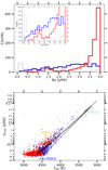 |
Fig. 1. Upper panel: distribution of our sample of stars as a function of Δν, with red giants in blue and He-burning stars in red. Stars with unidentified or uncertain evolutionary stage are plotted in grey. The inset is a zoom-in portion of the large panel. Lower panel: seismic diagram of our sample of stars with the same colour code as in the upper panel, where 1/νmax is a proxy for the luminosity. The solid black line is the evolutionary track of a 1 M⊙ model computed with MESA, using the 1M_pre_ms_to_wd test suite case. Some key events are highlighted: the RGB bump (RGB-b), the luminosity tip of the RGB (RGB-tip), and the AGB bump (AGB-b). |
In order to identify the evolutionary status, we used two classification methods. The first method is based on the estimate of differences between RGB stars and He-burning stars in the pressure-mode pattern, mainly through the acoustic offset ε (Kallinger et al. 2012). The second method is based on the estimate of differences in the envelope autocorrelation function (Mosser et al. 2019). However, the disagreement between these two classification methods rapidly grows at low Δν. For example, we reach 35% disagreement for 112 stars having Δν ≤ 1.0 μHz. Accordingly, we decided to only retain the evolutionary status so obtained if both classification methods agree.
3. Method
Acoustic modes dominate in the oscillation spectrum of evolved RGB and AGB stars. Gravity-dominated mixed modes start to disappear in the oscillation spectrum when Δν ≤ 3 μHz because of their high radiative damping and inertia (Dupret et al. 2009). The oscillation pattern of evolved stars can then be described by the asymptotic expression of the frequency of acoustic modes (Eq. (1)).
3.1. Adjusting the mode frequencies νn, ℓ
3.1.1. Best-matching template spectrum
The first step to be performed is the identification of the modes in the oscillation spectrum, which is ensured by using Eq. (1). First, we refined the analysis of the observed spectrum as follows. The background component that is dominated by the stellar granulation (Michel et al. 2008) was parametrised in the vicinity of νmax by a power law of the form
 (2)
(2)
where Bmax and αB are free parameters (Mosser et al. 2012). Then, we divided the observed spectrum by the background contribution. For the sake of visibility, we reduced the stochastic appearance of the oscillation pattern by smoothing the spectrum with a Gaussian function, for which the full width at half maximum (FWHM) is FWHM = d02Δν/4. We estimated d02 following an iterative process, starting with a rough estimate extracted from the scaling relation d02 = 0.162 − 0.013 log Δν (Mosser et al. 2013b).
Second, we built a template spectrum composed of radial, dipole, and quadrupole pressure modes located at the pressure mode frequencies derived from Eq. (1). The seismic parameters ε and d0ℓ were set following a scaling relation of the form A + B log Δν, where the guess values of A and B were taken from Mosser et al. (2013a). Then, the modes were modelled by Lorentzian functions. The heights of the Lorentzian functions were fixed by the underlying power excess distribution, which we modelled by a Gaussian function centred on the frequency of maximum oscillation power νmax (Mosser et al. 2012). Furthermore, the curvature term was set following the curvature of the red giant radial oscillation pattern as follows (Mosser et al. 2013b):
 (3)
(3)
We did not adjust the parameters in the expression of α since precise measurement of α is not crucial (Vrard et al. 2015). Finally, we found the best-matching template spectrum by computing the maximum cross-correlation with the smoothed spectrum. Then, the observed mode frequencies were identified at the local maxima close to the optimised frequency pattern. When mixed dipole modes were present, the most intense of the closest modes of the expected pure-pressure mode was adjusted. We report that the best-matching template spectrum is less reliable when Δνobs ≤ 0.4 μHz. In this case, most spectra do not exhibit a clear and intense pattern of ℓ = 0, 1, 2 modes, making the mode identification difficult. Nevertheless, a mode identification could be performed for these stars by vertically stacking their power spectrum with increasing νmax (see e.g., Yu et al. 2020).
3.1.2. Detection thresholds
Because of the stochastic nature of the modes, some modes are not sufficiently intense to be detected. Once the best-matching template spectrum was found with the method described in Sect. 3.1.1, we obtained a set of candidate modes. Then, in order to reduce biases, we applied the robust detection method of Appourchaux et al. (2006) to this set. To this end, the most intense modes were selected by evaluating the SN function, which corresponds to the most restrictive detection threshold in terms of height-to-background ratio in the power spectrum (Appourchaux et al. 2006). SN reads
 (4)
(4)
where PH1 is the probability of accepting that the observed peak is a mode and sdet is the rejection level relative to noise. We chose PH1 such that the height-to-background ratio SN reached 20 when sdet = 8, and the rejection level sdet was defined by
 (5)
(5)
where T is the observation time in units of 106 s, Δν is given in μHz, and pdet is the rejection probability that we kept equal to 5%. Second, we retained the candidate mode frequencies that were close to the expected pressure-mode frequencies with a less restrictive height-to-background ratio, which is given by Eq. (5). Owing to the small amplitudes of the ℓ = 3 modes due to geometric cancellation, we used a less restrictive detection threshold for the ℓ = 3 modes. The threshold for selecting ℓ = 3 modes is 25% lower than for the other degrees.
3.2. Glitch inference
When the best-matching template spectrum is found, we can search for the signature of glitches. To extract the signature of the helium second-ionisation zone in evolved giants, we followed the same technique as Vrard et al. (2015) for less evolved giants. As the oscillation spectrum of evolved red giants shows a limited number of radial orders, we calculated the frequency difference considering all degrees as follows:
 (6)
(6)
which is different from Eq. (4) of Vrard et al. (2015) because it is only based on radial modes. The frequency reference for these local large frequency separations was taken as the mid-point between consecutive mode frequencies. We isolated the glitch signature  by computing the difference between the measured and the expected local large frequency separations according to the universal pattern (Eq. (1))
 (7)
(7)
with  (Mosser et al. 2013b). We then fitted a damped oscillatory component of
  according to
 (8)
(8)
where 𝒜 and 𝒢 are the amplitude and the period of the modulation expressed in units of Δν, respectively, and Φ is the phase centred on νmax (Vrard et al. 2015). Many studies have used a more complicated function for the amplitude of the modulation. As we are restricted by the low number of observed modes, we preferred to use a simple frequency-dependent amplitude as was used before in the study of the base of the solar convective zone (Monteiro et al. 1994).
In evolved giants, quadrupole modes essentially behave as pure pressure modes. The case of dipole modes is complicated: They are most often reduced to a pressure-dominated mixed mode or to a cluster of modes very close to the pressure-dominated mixed mode. Because in most cases we have no way to identify the mixed-mode pattern, in practice we also consider dipole modes as pure pressure modes. This hypothesis is discussed below. We can add them in the fit of the glitch modulation without deteriorating the fit of the modulation. Then, the Nyquist criterion, which states that the frequency of the modulation must be strictly less than half the sample rate, writes 𝒢 ≥ 1 instead of 𝒢 ≥ 2 when only radial modes are used. When Δν ⪆ 3 μHz, dipole modes are no longer pure-pressure modes. It has been shown that adding the dipole modes of lowest inertia in each Δν range could bias the fit of the modulation, especially for the least evolved red giants (Broomhall et al. 2014; Dréau et al. 2020). Nevertheless, for the range of Δν we consider here, Broomhall et al. (2014) reported that the use of dipole modes of lowest inertia remarkably improves the robustness of the fit. When mixed modes are present, we then took into account the most intense dipole mode of the modes closest to the expected location of the pure-pressure mode.
3.3. Computation of mode visibilities
We investigated the energy distribution among modes of different degree ℓ in the case of evolved stars. The technique we used to compute the mode visibilities is described in Mosser et al. (2012). First, we computed the total mode energy, noted  , for which the radial order n lies between the lowest and highest observed radial orders. This was done by subtracting the background component and integrating the power spectral density over the whole spectral range where the mode is expected, that is, around the p-mode frequency inferred from Eq. (1) (see Table 1 and Fig. 2). Then we computed the visibility
  of a mode of degree ℓ as
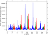 |
Fig. 2. Oscillation spectrum of the star KIC 2695975 (Δν = 1.538 μHz, and νmax = 10.11 μHz), with an emphasis on the spectral range where the power spectral density is integrated for each mode. Red, blue, green, and light blue are associated with radial, dipole, quadrupole, and octupole modes, respectively. This star has been classified as an RGB star with the two identification methods adopted in this work. |
Boundaries for the integration of the power spectral density.
 (9)
(9)
where  is the squared amplitude of the mode of degree ℓ.
When mixed modes are present, the procedure was the same: The energy  corresponds to the total energy of the mixed modes associated with the radial order n. The errors on the visibilities were computed from the errors on the boundary frequencies listed in Table 1: The energy contained in the 1σ error region of the boundary frequencies is interpreted as the error on the parameter
  .
.
3.4. Mode fitting
The mode amplitudes and widths derived from the fit of the modes provide unique constraints on the mode excitation and damping. In this context, we adopted a frequentist approach. The modes were fitted with Lorentzian profiles following the maximum likelihood estimator technique described in Toutain & Appourchaux (1994). The fit was performed radial order by radial order, so that we have three modes at most to fit per iteration. Owing to their very low amplitudes, ℓ = 3 modes cannot be fitted. Radial, dipole, and quadrupole modes were fitted on top of the background using
 (10)
(10)
where Hn, ℓ, νn, ℓ, and Γn, ℓ are the height, frequency, and width of the mode of radial order n and degree ℓ, respectively. We point out that the background was extracted separately, and we kept it fixed when fitting the modes. The mode amplitude can be deduced from the mode height and the width by
 (11)
(11)
Because of the low signal-to-noise ratios, the presence of mixed modes, and the stochastic excitation, some modes were not correctly fitted. The measurements were rejected when the width was too close to the frequency resolution (i.e., when Γn, l ≤ 1.1δνres) or when the width was overestimated (i.e., when Γn, l ≥ Δν/7). When mixed modes were present, we fitted the closest mixed modes to the expected pure-pressure mode. Then, following Benomar et al. (2014), Belkacem et al. (2015), and Mosser et al. (2018), we inferred the mode width and the mode amplitude that the mode would have if it were purely acoustic through
 (12)
(12)
where ζ depends on the inertia of the fitted mixed mode. Characterising the mixed-mode pattern is beyond the scope of this work. However, we estimated the mode inertia that is defined in Mosser et al. (2018), for example, using scaling relations (Eqs. (17) and (18) from Mosser et al. 2017a for the coupling factor q and the database from Vrard et al. 2016 for the period spacings ΔΠ1).
We finally computed the mean mode amplitude ⟨Aℓ⟩ using the three p modes of degree ℓ closest to νmax. We corrected the wavelength dependence of the photometric variation integrated over the Kepler bandpass according to
 (13)
(13)
where TK = 5934 K (Ballot et al. 2011a). The average mode width ⟨Γℓ⟩ was computed as the weighted mean of the three p modes of degree ℓ closest to νmax, where the mode amplitude was used as weight (see e.g., Vrard et al. 2018).
4. Results
In this section, we characterise the oscillation spectrum of evolved giants as precisely as possible. We compare our measurements with previous studies that focused on less evolved stages and with theoretical predictions.
4.1. Acoustic offset ε and reduced small separations d0ℓ
From the fit of the spectrum described by Eq. (1) we derived the global acoustic offset ε and the reduced small separations d0ℓ associated with the detected modes (see Fig. 3). Scaling relations were adjusted to our sets of seismic parameters in the form Aℓ + Bℓ log(Δν), where Aℓ and Bℓ are free parameters that are summarised in Table 2, and Δν is given in μHz.
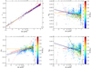 |
Fig. 3. Seismic parameters of the asymptotic pattern of red giants (Eq. (1)) after adjusting Δν with the best-matching template following the procedure described in Sect. 3. Upper left panel: acoustic offset ε as a function of Δν, where blue triangles indicate RGB stars and red diamonds He-burning stars. Stars with either an unidentified evolutionary stage or disagreement between the two classification methods described in Sect. 2 are represented in grey. Upper right panel: reduced small separation d02 as a function of Δν; the stellar mass is colour-coded. Bottom panels: same labels as for the upper right panel, but for d01 and d03 as a function of Δν. The solid blue and red lines are the median values in 0.4 μHz Δν bins for low-mass stars (M ≤ 1.2 M⊙) and for high-mass stars (M ≥ 1.2 M⊙), respectively. The dashed orange lines represent the scaling relations from Mosser et al. (2013a), and the solid dark blue lines are the scaling relations derived in this study (listed in Table 2). The dot-dashed pink and dark green lines correspond to the scaling relations for less evolved stars from Corsaro et al. (2012) and Huber et al. (2010), respectively. Mean error bars estimated at low Δν (Δν ≤ 1.0 μHz) and at high Δν (Δν ≥ 1.0 μHz) are represented at the bottom of each panel. |
Fit of the seismic parameters ε and d0ℓ, and the dimensionless glitch parameters.
4.1.1. Acoustic offset ε
The oscillation spectrum of radial modes is depicted by the global acoustic offset ε as shown in Fig. 3. The trend that we observe for RGB stars is similar to what has been obtained in previous studies (Mosser et al. 2013a; Yu et al. 2020). With our method, which uses a global fit of the oscillation pattern, we derive similar values of ε for RGB and He-burning stars, in contrast to Kallinger et al. (2012), who used a local approach. As they showed, the glitches have limited effect on global measurements of the seismic parameters but they affect local measurements considerably. In Sect. 4.2 we investigate the local effects on the mode frequencies by studying the modulation left by the helium second-ionisation zone in p-mode frequencies.
4.1.2. Reduced small separations d0ℓ
Theoretical models predict that the effects of stellar evolution are reflected in the reduced small separations d0ℓ. They are sensitive to any internal structure change that affects the gradient of the sound speed (Tassoul 1980; Roxburgh & Vorontsov 2003) in the deep interiors. While a star ascends the RGB, the stellar core contracts but does not undergo important structure changes. Therefore the reduced small separations vary only slowly along the RGB.
Figure 3 shows that d01 decreases when Δν decreases, as observed by previous observational studies on less evolved stars (Huber et al. 2010; Corsaro et al. 2012; Mosser et al. 2013a). This points out the fact that during stellar evolution, dipole p modes approach the doublet formed by ℓ = 0 and ℓ = 2 modes, in agreement with theoretical models (Montalbán et al. 2010; Stello et al. 2014). The variation of d01 during late stellar evolution can be linked to the location of the turning points of ℓ = 1 modes. By examining the structure of low-mass red giant models, Montalbán et al. (2010) found that d01 takes negative values when the turning points of ℓ = 1 modes are deep in the convective envelope. This is exactly what we observe and allows us to extend the interpretation made for RGB stars to AGB stars, which have negative d01. Stellar models of Montalbán et al. (2010) also predict that core-He-burning stars have both positive and negative d01, and that the turning points of ℓ = 1 modes are located inside the radiative region. The determination of d01 in clump stars is more difficult because the observed large spread in d01 mainly reflects the presence of mixed modes that perturb the adjustment of the acoustic dipole modes.
The reduced small separation d02 is sensitive to the structure differences between core He-burning stars and RGB stars: We report that d02 is larger on average for core He-burning stars than for RGB stars, as has been reported by Kallinger et al. (2012). We note a clear mass effect: the lower the mass, the larger d02. The first evidence of this mass dependence in red giants has been discussed in Huber et al. (2010), in agreement with the theoretical models (Montalbán et al. 2012). We find that this mass dependence is also visible for d01 and d03, as predicted by the theoretical models of Montalbán et al. (2010), despite the presence of mixed modes that cause the values of these parameters to become more scattered. However, Montalbán and collaborators did not discuss the origin of this mass dependence. Further work is therefore needed to physically understand this behaviour.
As for ℓ = 3 modes (see the bottom panel of Fig. 3), we note that the reduced small separation d03 increases when Δν decreases, as shown by the observations of Kepler (Huber et al. 2010) and stellar models (Montalbán et al. 2010). This expresses the fact that the ℓ = 3 modes approach the left-hand side of ℓ = 0, 2 modes during stellar evolution. Further theoretical work is needed to investigate and understand this behaviour.
4.2. Signature of the helium second-ionisation zone
The results obtained after fitting the modulation left by the helium second-ionisation zone in Δνn, ℓ are shown in Fig. 4. In Table 2 we present the scaling relations found for the dimensionless amplitude 𝒜 and period 𝒢, computed for RGB stars alone, in the form CΔνD, where C and D are free parameters and Δν is given in μHz.
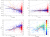 |
Fig. 4. Modulation amplitude 𝒜, modulation period 𝒢, and modulation phase Φ as a function of Δν, with the same labels as in Fig. 3. The thick solid lines are the median values in 0.5 μHz Δν bins, shown in blue for RGB stars and in red for He-burning stars. In the upper panels, dashed blue lines are the fits presented in Table 2. In the upper left panel, the dashed orange line is the fit obtained for less evolved stars (Vrard et al. 2015), corrected with a factor that accounts for the differences between the methods we used to fit the modulation as described in Sect. 4.2. In the upper right panel, dotted black lines delimit the domain of reliable measurements of 𝒢, which are described in Sect. 3, and the thin solid line is the modulation period inferred from MESA models for a 1 M⊙ star and starting from the RGB up to the AGB. The error bars are computed in the same way as in Fig. 3. In the lower right panel, the stellar mass is colour-coded, and medians are represented by solid lines for low-mass stars (M ≤ 1.2 M⊙) and by dashed lines for high-mass stars (M ≥ 1.2 M⊙). Because Φ varies with stellar evolution, we calculated the medians for RGB and He-burning stars separately. We show them in blue for RGB and in red for He-burning stars. |
4.2.1. Modulation amplitude 𝒜
When a star ascends the RGB or AGB (Δν ≲ 3 μHz for the early AGB), the dimensionless amplitude of the modulation 𝒜 notably increases. During the clump phase, it is more difficult to conclude because of the large spread of the amplitudes. We verified that most of the stars with 𝒜 ≥ 0.09 also have a dim Kepler magnitude, hence their oscillation spectrum is recorded with a low signal-to-noise ratio, so that the measurement of 𝒜 is quite noisy. Globally, the amplitude of the modulation is larger for He-burning stars than for RGB stars. This is consistent with the results presented in Vrard et al. (2015) between clump and RGB stars having Δν ≥ 3.0 μHz. We note that the values of the modulation amplitude are larger in our work than in Vrard et al. (2015), as expected from the different methods with which Δνn, ℓ and δg, obs(n, ℓ) were computed. To compare our results with those of Vrard et al. (2015), we then estimated how different the modulation amplitudes are between the two methods. We note that our modulation amplitudes are 1.8 times larger on average than those extracted in Vrard et al. (2015). Then, we multiplied the fit reported in the latter study by 1.8 and compared it with ours, as plotted in the upper left panel of Fig. 4. Our results are also consistent with stellar evolution models that indicate that the difference observed in the modulation amplitude 𝒜 between RGB and He-burning phases is correlated with a difference of temperature and density at the level of the helium second-ionisation zone (Christensen-Dalsgaard et al. 2014).
4.2.2. Modulation period 𝒢
We note that the modulation period 𝒢 slightly decreases throughout the stellar evolution (Fig. 4). This means that the helium ionisation zone slowly sinks into the stellar interior during evolution, as predicted by stellar models (Fig. 6 of Broomhall et al. 2014). The typical period does not globally differ between He-burning stars and their RGB counterparts. Our measurements were compared to the results derived with the stellar evolution code Modules for Experiments in Stellar Astrophysics (MESA) using the 1M_pre_ms_to_wd test suite case (Paxton et al. 2011, 2013, 2015, 2018, 2019). In Appendix A we describe how we extracted the modulation period 𝒢 from stellar models. Stellar models indicate that RGB stars and He-burning stars of the same mass and same large separation should have the same modulation period 𝒢, in agreement with observations. However, He-burning stars have more scattered 𝒢 values than their RGB counterparts. The large spread does not appear to stem from the presence of mixed modes because Vrard et al. (2015) also reported a spread like this for clump and RGB stars, although they only used radial modes in the modulation fits. As reported for the modulation amplitude 𝒜, the spread is rather well explained by the dim magnitudes, hence by the low signal-to-noise ratios in the oscillation spectra.
4.2.3. Modulation phase Φ
The modulation phase Φ differs depending on the evolutionary stage. By letting the phase vary in the interval [ − π, +π], we observe that He-burning stars globally show a negative phase difference compared to their H-burning counterparts. This difference has been reported by Vrard et al. (2015) for clump and RGB stars. The authors showed that the phase difference is related to the difference in ε reported in the study of Kallinger et al. (2012) between clump and RGB stars. The link between Φ and ε, which depends on the evolutionary stage, is discussed in Sect. 5. Similarly to the modulation amplitude 𝒜 and the modulation period 𝒢, the spread of the modulation phase Φ is larger for He-burning stars than for H-burning stars. We verified that the spread of Φ becomes important when the Kepler magnitude exceeds 11. The large spread of Φ could then be explained by low signal-to-noise ratios in the oscillation spectra.
4.2.4. Mass dependence of the glitch parameters
We also investigated the stellar mass dependence of the glitch modulation parameters. We find evidence of a mass dependence for the modulation amplitude, which varies as 𝒜RGB ∝ Δν−0.41 ± 0.01M−0.34 ± 0.02 on the RGB with a similar dependence during He-burning phases. Conversely, the modulation period is weakly correlated with the stellar mass on the RGB and follows 𝒢RGB ∝ Δν−0.05 ± 0.01M−0.04 ± 0.01, while it is practically independent of the stellar mass during the He-burning phase. The mass dependence of the modulation phase Φ is illustrated in Fig. 4. We note a negative phase difference between low-mass and high-mass RGB stars for Δν ≤ 2.0 μHz. The lack of data for He-burning stars at low Δν prevents us from drawing any conclusion. In case of less evolved stars, Vrard et al. (2015) did not find any correlation between the stellar mass and the glitch parameters, except for the modulation phase for clump stars. These mass dependences remain empirical, and further theoretical work is needed to determine their physical basis.
4.3. Mode widths
The mode widths ⟨Γℓ⟩ were fitted by the function
 (14)
(14)
where aℓ and bℓ are free parameters. The fits are presented in Fig. 5 and summarised in Table 3.
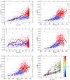 |
Fig. 5. Upper panels: ⟨Γ0⟩ as a function of Δν and Teff. Middle panels: ratio of ⟨Γ1⟩ and ⟨Γ0⟩ as a function of Δν and ⟨Γ1⟩ as a function of Teff. For convenience, horizontal dotted black lines are plotted at specific values of 0.5, 1.0, 1.5, and 2.0. Bottom left panel: ⟨Γ2⟩ as a function of Teff. The colours and symbols are the same as in Fig. 4. Mean error bars on the widths have been computed both at low Teff (Teff ≤ 4200 K) and at high Teff (Teff ≥ 4200 K). These limits are equivalent to the limits in Δν chosen in Fig. 3. The fits presented in Table 3 are plotted with dashed light blue lines for RGB stars. Bottom right: ⟨Γ1⟩ as a function of Δν with the dipole mode visibilities colour-coded. The solid and dashed lines correspond to the median values for low-visibility dipole modes ( |


Scaling relations for the mode widths and for the mode amplitudes.
We note that clump stars globally have larger radial mode widths with a larger spread than those observed for RGB stars, as mentioned in previous studies (Corsaro et al. 2012; Vrard et al. 2018). However, when core-He-burning ends and the star ascends the AGB (Δν ≲ 3 μHz), the radial mode widths decrease and become comparable to measurements made on the RGB.
In Fig. 5 we compare the dipole mode widths ⟨Γ1⟩ to the radial mode widths ⟨Γ0⟩. On the RGB, we note that ⟨Γ1⟩ values are globally 20% higher than ⟨Γ0⟩ above Δν ≥ 3.5 μHz, while they are globally similar below. For He-burning stars, the ℓ = 1 modes have larger widths than the ℓ = 0 modes above Δν ≥ 1.5 μHz. We identified three reasons that might explain this behaviour. First, as mentioned in Sect. 3, we applied the correction expressed by Eq. (12) to ⟨Γ1⟩ when the fitted modes are mixed modes. However, the term ζ is close to 1, therefore the correction to ⟨Γ1⟩ introduces large uncertainties on the inferred dipole p-mode widths. Second, most of the unexpectedly high ⟨Γ1⟩ values are in fact highly perturbed by mixed modes. Gravity-dominated mixed modes can only be observed if the condition
 (15)
(15)
is met (Mosser et al. 2018), where 𝒩 = Δν/(ν2ΔΠ1) is the number of gravity modes per radial order n, ΔΠ1 is the period spacing, q is the coupling factor, Γ0 is the radial mode width, and δνres is the frequency resolution. Using typical values of q (see e.g., Mosser et al. 2017a) and ⟨Γ0⟩, we can infer that the right-hand side term of Eq. (15) is close to 20 at Δν ∼ 3 μHz for He-burning stars. Then, Eq. (15) is hardly verified and only p-dominated modes are mainly visible. In these cases, the mixed modes are so close that the fits rather reproduce several confused mixed modes than a unique pure pressure mode. Third, we note that all the highest values of ⟨Γ1⟩ are systematically associated with low ℓ = 1 mode visibilities in the interval Δν ∈ [1.5, 2.5] μHz. These dipole modes with a low amplitude are unexpectedly large and are further discussed in Sect. 5.3. The comparison between ⟨Γ2⟩ and ⟨Γ0⟩ is not discussed here because ⟨Γ0⟩∼⟨Γ2⟩, as expected.
We also investigated the temperature dependence of ⟨Γℓ⟩ (Fig. 5). The fits performed on each stellar population (cf. Table 3) indicate that ⟨Γℓ⟩ and Teff are strongly correlated, regardless of the degree ℓ. Vrard et al. (2018) also reported that ⟨Γ0⟩ is correlated with Teff for less evolved giants, but this correlation is not as pronounced as in the present study. A strong correlation like this is expected across the HR diagram according to theoretical work (Belkacem et al. 2012).
4.4. Mode amplitudes
The radial mode amplitude ⟨A0, bol⟩ defined in Eq. (13) is plotted as a function of νmax in Fig. 6 and was adjusted by the scaling relation
 (16)
(16)
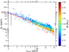 |
Fig. 6. Radial mode amplitude ⟨A0, bol⟩ computed from Eq. (13) as a function of νmax with the stellar mass colour-coded. The dashed lines are the fits presented in Table 3, shown in blue for low-mass stars (M ≤ 1.2 M⊙) and in red for high-mass stars (M ≥ 1.2 M⊙). The error bars are computed in the same way as in Fig. 5. |
where cℓ and dℓ are free parameters and νmax is given in μHz. The radial mode amplitudes follow the same trend as highlighted in recent studies (e.g., Huber et al. 2011; Stello et al. 2011; Mosser et al. 2012; Vrard et al. 2018). The radial mode amplitude does not differ between RGB stars and He-burning stars. For both stellar populations, the radial mode amplitude follows a power law with an exponent roughly equal to −0.70. Furthermore, the previous studies reported a clear mass dependence regardless the evolutionary stage: the higher the mass, the lower the radial mode amplitude (see Fig. 6).
4.5. Mode visibilities
The energy distribution between modes of different degree ℓ can be studied through the mode visibilities (Eq. (9)). They are presented in Fig. 7 and were fitted by the linear function
 (17)
(17)
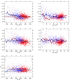 |
Fig. 7. Upper panels: visibility of the ℓ = 1 modes as a function of Teff in the left panel and of νmax in the right panel. The colours and symbols are the same as in Fig. 5. The error bars are computed in the same way as in Fig. 5. Similarly, error bars on the visibilities are given for both low νmax (νmax ≤ 4.5 μHz) and high νmax (νmax ≥ 4.5 μHz). The dashed lines are the fits presented in Table 4, in light blue for RGB stars and in light red for He-burning stars. The thin solid light blue and light red lines are the fits obtained for less evolved stars (Mosser et al. 2012) for RGB stars and for He-burning stars, respectively. The thin solid black line is the theoretical prediction (Ballot et al. 2011b). Middle panels: same labels as in the upper panels, but for the visibility of ℓ = 2. Lower left panel: same labels as in the upper left panel, but for the visibility of ℓ = 3 modes. The median values are computed in 50 K wide Teff bins and in 1.5 μHz wide νmax bins. |
where α and β are free parameters and Teff is given in K (see Table 4).
We verified that the high values of  and
and  can be explained by very weak radial mode amplitudes. For some He-burning stars, the dipole mixed modes extend up to the frequency range where ℓ = 3 modes are located. When mixed modes are too close to the ℓ = 3 modes, a fraction of the energy associated with mixed modes can be accidentally accounted for as part of the energy of ℓ = 3 modes. Consequently, some
  values may be underestimated, and
  is inevitably overestimated. In the case of less evolved stars, Mosser et al. (2012) suggested that the scatter in
  could be related to the conditions that govern the coupling between g modes and p modes, giving rise to mixed modes. In the case of He-burning stars, this could explain the spread we obtain because these stars clearly exhibit mixed modes when Δν ≳ 3.0 μHz.
Although we note a large spread for the mode visibilities, it is clear that the non-radial mode visibilities increase when Teff decreases both for RGB stars and He-burning stars, as expected from theoretical predictions (Ballot et al. 2011a). The only exception is the visibility of ℓ = 1 modes in He-burning stars. This is due to the presence of several dipole modes with very low visibilities in the interval Teff ∈ [4200, 4500] K, as reflected by the gap between the medians computed for RGB and He-burning stars. The mode visibilities in evolved stars similarly behave as in less evolved stars, except in the case of ℓ = 3 modes, since we note that  increases towards low Teff, whereas Mosser et al. (2012) observed the opposite trend.
The visibility of dipole modes  is represented as a function of νmax in the upper right panel of Fig. 7. We observe a clear difference between RGB stars and He-burning stars in the interval νmax ∈ [7, 20] μHz, with He-burning stars having weaker
  than their RGB counterparts. In parallel, we previously reported that Γ1 is greater for He-burning stars in this interval (Fig. 5). It is certain that mixed modes perturb the extraction of the pure pressure dipole mode widths when Δν ≥ 1.5 μHz, but the presence of low-visibility dipole modes reflects a shortage of dipole mode energy, which could be linked to a higher dipole mode damping, hence to a higher dipole mode width. We study this question in Sect. 5. Furthermore, we find that quadrupole modes have larger amplitudes in the H-burning phases than on the He-burning phases in the interval νmax ∈ [15, 35] μHz, as represented in the middle right panel of Fig. 7. This difference may be linked to the mixed character of the quadrupole modes, which is more pronounced during the clump phase in the interval νmax ∈ [15, 35] μHz.
Nevertheless, we note a large spread of the dipole mode visibilities. The dipole mode visibilities of He-burning stars become comparable with those measured on the RGB at low Δν (Δν ≤ 1.5 μHz), when mixed modes disappear in the oscillation spectrum. The physical mechanisms that govern the coupling between the p-mode and the g-mode cavities might therefore be linked to the observation of low dipole mode visibilities. Even if the presence of depressed modes in advanced stages of stellar evolution is not clear, the simultaneous presence of low dipole mode visibilities and dipole mixed modes could help to identify the physical processes that cause the depressed modes in less evolved stages, which are still under debate (Fuller et al. 2015; Stello et al. 2016; Cantiello et al. 2016; Mosser et al. 2017b).
4.6. Comparison with other peak-bagging methods
The measurements inferred from our frequentist peak-bagging are compared with those4 of the automated Bayesian peak-bagging algorithm Aorigin=c]180BBA (Kallinger 2019), which uses the Bayesian nested sampling algorithm MULTINEST (Feroz et al. 2009). The average radial mode widths and bolometric amplitudes derived in the Bayesian approach were computed in the same way as in Sect. 3.4. The comparison is shown in Fig. 8.
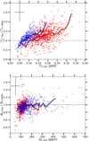 |
Fig. 8. Top panel: ratio of the average radial mode widths ⟨Γ0⟩ obtained in this study and those obtained with a Bayesian method (Kallinger 2019). The median values are computed in 0.015 μHz wide Γ0, freq bins. Bottom panel: same as in the upper panel, but for the average radial mode bolometric amplitude ⟨A0, bol⟩. The colours and symbols are the same as in Fig. 4. The median values are computed in 20 ppm A0, freq bins. The dotted line represents the 1:1 agreement. Mean error bars are represented at the top of each panel. |
The radial mode widths ⟨Γ0⟩ derived with our frequentist peak-bagging are globally larger than those obtained with Aorigin=c]180BBA by about 25%. This overestimate is frequency dependent because it increases for higher values of ⟨Γ0⟩. Conversely, our radial bolometric mode amplitudes are weakly underestimated by about 5% with respect to the Aorigin=c]180BBA values. Vrard et al. (2018) also reported that the radial mode width was overestimated by about 10% in the frequentist approach with respect to a Bayesian approach. Moreover, we approximated the background component by Eq. (2) around νmax, while Kallinger (2019) modelled it with two super-Lorentzian functions (Kallinger et al. 2014). The background parametrisation has a non-negligible impact on the mode fitting, and stellar background bias is one of the main sources of frequency-dependent systematic errors in the measurements of mode widths and heights (Appourchaux et al. 2014). The way that the stellar background was modelled may therefore partly explain the differences we find between measurements.
5. Discussion
5.1. Stellar classification at advanced stages
Using a global measurement of the large separation Δν and the oscillation pattern of red giants (Eq. (1)), we did not find any difference in the acoustic offset ε between RGB stars and He-burning stars. In parallel, we highlighted a difference in the signature of the helium second-ionisation zone between these stellar populations, especially in the modulation phase Φ. This phase difference locally affects the measurement of Δν according to Eq. (7). A local change in Δν can be linked to a local change in ε by differentiating Eq. (1), leading to
 (18)
(18)
In the case of RGB and clump stars, Vrard et al. (2015) showed that the values of δε inferred from δ(log Δν) that is related with the helium second-ionisation zone match the typical difference in ε between RGB and clump stars. They identified the glitch signatures as the physical basis of the stellar population identification method based on the acoustic offset ε. We extended the conclusions raised by Vrard et al. (2015) to more advanced evolutionary stages, that is, between RGB and He-burning stars, including clump and AGB stars. The difference in the local measurements of ε between RGB and AGB stars reported by Kallinger et al. (2012) is caused by the different glitch signature of the helium second-ionisation zone, especially for the modulation phase Φ.
5.2. AGB bump
After leaving the clump phase where helium-burning takes place in the core, the star enters the AGB phase. During the early asymptotic giant branch (eAGB) and in the case of low-mass and intermediate-mass stars, two turning-backs of the evolutionary track can be seen in a narrow interval of luminosity, similarly to what can be seen during the RGB bump: This is the so-called AGB bump (AGBb). It is caused by the onset of the shell-He burning and was first identified in the Large Magellanic Cloud colour–magnitude diagram (Gallart 1998). The AGBb is observationally characterised by a local excess of stars in the luminosity distribution of stellar populations. Such an increment has been identified at log(L/L⊙) ∼ 2.2 (Bossini et al. 2015). For a star of M = 1.0 M⊙ and Teff = 4500 K, this is equivalent to νmax ∼ 8 μHz according to the scaling relation (Kjeldsen & Bedding 1995)
 (19)
(19)
Accordingly, we selected He-burning stars that left the clump phase (i.e., νmax ≲ 25 μHz). Their distribution as a function of νmax is shown in Fig. 9. By tracking stellar evolution towards low νmax, we note a depleted region followed by a peak for low mass-stars (at νmax ∼ 8 μHz) and for high-mass stars (at νmax ∼ 11 μHz). The depleted region could be explained by a difference in the evolution speed. We have computed models with the MESA code, using the 1M_pre_ms_to_wd test suite case to investigate the evolution speed between the end of the clump phase and the ascent on the AGB. The results are presented in the right panel of Fig. 9. For a given mass, we note that the evolution is faster between the end of the clump phase and the start of the AGBb than right after the AGBb since the variation of νmax with time is more important before the AGBb. The fast evolution speed before the AGBb results in a small statistical probability to meet low-mass stars in the interval νmax ∈ [8, 15] μHz and high-mass stars in the interval νmax ∈ [14, 18] μHz. Investigating the AGBb in depth is part of our future work.
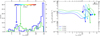 |
Fig. 9. Left panel: distribution of He-burning stars in terms of νmax. In blue we show the number of low-mass He-burning stars (M ≤ 1.2 M⊙), and in green we show the number of high-mass He-burning stars (M ≥ 1.2 M⊙). The colour bar indicates the location in νmax where we expect the AGB bump for a given mass following Eq. (19) and adopting Teff = 4800(νmax/40.0)0.06 (Mosser et al. 2010). The blue and green arrows roughly indicate the location of the AGB bump for low-mass and high-mass stars, respectively, which is characterised by a local excess of stars. Right panel: Evolution speed dνmax/dτ, where τ is the stellar age, as a function of νmax for different stellar masses. The models computed with MESA start from the end of the clump phase, which is marked by a diamond. The start and the end of the AGB bump are marked by a circle and a star, respectively. |
5.3. A strong damping during the eAGB phase?
Very low degree modes have similar eigenfunctions in the stellar outer layers, so that they are excited in similar conditions and show similar power spectral densities. However, as mentioned in Sect. 4.5, many He-burning stars have very low dipole mode visibilities below νmax = 20 μHz. In parallel, we found that most of the He-burning stars with low dipole mode visibilities have larger dipole mode widths. These low dipole mode visibilities reflect a lack of energy that could be linked to a strong dipole mode damping. Accordingly, we analysed the correlation between low visibility and large damping of dipole modes in detail by fitting the mixed-mode pattern during the early-AGB phase.
To this end, we considered single stars that have been identified as eAGB stars according to the classification method of Mosser et al. (2014). We selected five eAGB stars that have both low visibility dipole modes and a mixed-mode pattern clear enough to fit individual mixed modes and measure their widths (KIC 6847371, 11032660, 5461447, 10857623, and 6768042). We compared these widths to the pure-pressure dipole-mode width with Eq. (12). The results shown in Appendix B are unfortunately not unequivocal. Three of these eAGB stars present a strong dipole-mode damping, which is within the 1σ uncertainty for KIC 6847371 and KIC 5461447 and within the 2σ uncertainty for KIC 11032660. Nevertheless, this is not what we observe for KIC 10857623 and KIC 6768042. We face several constraints to reduce the uncertainties (or to fit other spectra), such as a low signal-to-noise ratio, a high ratio ζ of the mode inertia in the core and the total mode inertia (which leads to high uncertainties through Eq. (12)), limited frequency resolution, rotational splittings, and buoyancy glitch signature. We therefore tested another method to process these constraints together.
In a star in spherical equilibrium (thus non-rotating and without magnetic field), we expect the energy equipartition between modes of even and odd degrees to be satisfied. The lack of energy observed for dipole modes can be studied by comparing the energy of even-degree modes to that of odd-degree modes. To this end, we computed the ratio between the visibilities of odd and even degrees,
 (20)
(20)
Modes that have a degree of same parity are close one to each other, as illustrated in Fig. 2. As a result, studying the global contribution of the energy then limits the impact of the energy leakage between individual degrees. We use the measurement of the odd/even visibility ratio as an indicator of the variation of the visibilities of ℓ = 1 modes (Fig. 10). The variation is in fact dominated by the dipole modes for two reasons. On the one hand, the visibility of the octupole modes is very low for geometrical reasons. On the other hand, the quadrupole modes essentially behave as pure pressure modes for evolved giants, and always have a more pronounced pressure character than dipole modes. Below νmax = 20 μHz, the energy equipartition seems to be invalid for He-burning stars. The dipole mode visibility is weaker than predicted by theory for He-burning stars. This lack of dipole mode energy is linked to a large dipole mode damping according to our study, and invalidates the energy equipartition between the different low-degree modes.
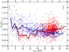 |
Fig. 10. Ratio of the mode visibilities of odd and even degrees as a function of νmax. Same labels as in Fig. 4. For convenience, horizontal dashed black lines are plotted at specific values of 0.75, 1.00, and 1.25. The error bars are computed in the same way as in Fig. 3. The median values are computed in 1.5 μHz νmax bins. |
For RGB stars we can note that the visibility of ℓ = 1 modes is globally lower at high νmax (see Fig. 7) and is especially lower than the expected value (1.54), which makes  greater than
  above νmax = 25 μHz. This difference was first observed by Mosser et al. (2012) for less evolved red giants and can theoretically be explained by a difference of dipole mode damping (Dziembowski 2012). The radiative damping causes an energy loss at the envelope base that decreases when the star ascends the RGB (Dziembowski 2012, see Figs. 6 and 7). For a star with an initial mass M0 = 2 M⊙, the energy loss by gravity wave emission at the envelope base is expected to cancel out when νmax ≃ 28 μHz on the RGB. This is consistent with our observations because we note that
  increases with evolution below νmax ≤ 28 μHz (see the upper right panel of Fig. 7). On the RGB, radiative damping may explain the damping of energy of dipole modes observed at high νmax. On the AGB, the dipole mode visibility evolves in the opposite direction. Given that the evanescent region between the g-mode and the p-mode cavities grows while the star ascends the AGB, mixed modes become less visible, and consequently, the only visible dipole modes are trapped in the envelope, as observed on the RGB. It might therefore be relevant to investigate the radiative damping in order to determine whether it can explain the damping of dipole modes on the AGB.
6. Conclusion
So far, we have performed the first exhaustive study of the seismic analysis of evolved giants, including ∼2000 stars ascending the RGB towards the luminosity tip and He-burning stars both in the clump phase and ascending the AGB. We successfully characterised the oscillation spectrum of stars with Δν ≥ 0.5 μHz and extracted the radial, dipole, and quadrupole mode parameters. By investigating the signature of the helium second-ionisation zone, we identified the physical origin on which the classification method based on ε and presented in Kallinger et al. (2012) relies at low Δν, that is, between RGB and AGB stars. We found that the amplitude and phase of the modulation introduced in the mode frequencies differ in RGB and in He-burning stars, that is, in core-He-burning and AGB stars. Work is in progress to investigate these differences with modelling. These differences affect local measurements of ε and enable classifying RGB and He-burning stars. Thus, we extended the work of Vrard et al. (2015), who drew the same conclusions, but considering RGB stars versus clump stars. As a consequence, we now have two methods relying on the same physical basis to decipher stellar evolution effects in evolved giant stars. On the one hand, we can adopt a local analysis where the signature of the helium second-ionisation zone is included in the acoustic offset ε. In this case, the possible values of ε reflect stellar evolution effects. On the other hand, we can adopt a global analysis where the values taken by ε are squeezed together and the stellar evolution effects in ε fade. However, in this case, we can still emphasise the stellar evolution effects by considering an additional term in Eq. (1) representing the signature of the helium second-ionisation zone on mode frequencies.
Having access to seismic diagnoses of evolved giants is promising for the understanding of stellar evolution, especially during the AGBb. The AGBb is expected to occur at log(L/L⊙) ∼ 2.2 after the core He-burning phase. The investigation of the AGBb will be approached in a forthcoming paper. Furthermore, we highlighted that after the core He-burning phase, (i) the evolution is faster for low-mass stars, (ii) the dipole mode energy decreases, and (iii) the pressure-mode damping slowly becomes comparable to that measured on the RGB. This suggests that other physical processes need to be investigated in order to understand the mode damping and the observed visibilities as soon as core He-burning stops, that is, when the core becomes radiative again.
We use the expressions shell-H-burning stars and RGB stars in an equivalent manner. Core-He-burning stars and shell-He-burning stars refer to clump and AGB stars, respectively. He-burning stars indistinctly refer to core-He-burning stars and shell-He-burning stars.
This central acoustic offset εc is a local measurement of ε that is computed with the central three radial modes that are closest to νmax.
Counterparts refer to stars that have the same Δν and νmax.
Acknowledgments
The authors are grateful to the anonymous referee who helped them in improving this paper with constructive suggestions. G.D. thanks P. Houdayer, R. Samadi and M. Vrard for fruitful discussions that helped improving this work. C.G. is supported by FCT – Fundação para a Ciência e a Tecnologia through national funds (PTDC/FIS-AST/30389/2017), by FEDER – Fundo Europeu de Desenvolvimento Regional through COMPETE2020 – Programa Operacional Competitividade e Internacionalização (POCI-01-0145-FEDER-030389), and by FCT/MCTES through national funds (PIDDAC) by these grants UIDB/04434/2020 and UIDP/04434/2020.
References
- Aarslev, M. J., Houdek, G., Handberg, R., & Christensen-Dalsgaard, J. 2018, MNRAS, 478, 69 [CrossRef] [Google Scholar]
- Appourchaux, T., Berthomieu, G., Michel, E., et al. 2006, in The CoRoT Mission Pre-Launch Status - Stellar Seismology and Planet Finding, eds. M. Fridlund, A. Baglin, J. Lochard, & L. Conroy, ESA SP, 1306, 377 [Google Scholar]
- Appourchaux, T., Chaplin, W. J., García, R. A., et al. 2012, A&A, 543, A54 [NASA ADS] [CrossRef] [EDP Sciences] [Google Scholar]
- Appourchaux, T., Antia, H. M., Benomar, O., et al. 2014, A&A, 566, A20 [NASA ADS] [CrossRef] [EDP Sciences] [Google Scholar]
- Baglin, A., Auvergne, M., Barge, P., et al. 2006, in The CoRoT Mission Pre-Launch Status - Stellar Seismology and Planet Finding, eds. M. Fridlund, A. Baglin, J. Lochard, & L. Conroy, ESA SP, 1306, 33 [Google Scholar]
- Ballot, J., Turck-Chiéze, S., & García, R. A. 2004, A&A, 423, 1051 [NASA ADS] [CrossRef] [EDP Sciences] [Google Scholar]
- Ballot, J., Barban, C., & van’t Veer-Menneret, C. 2011a, A&A, 531, A124 [NASA ADS] [CrossRef] [EDP Sciences] [Google Scholar]
- Ballot, J., Gizon, L., Samadi, R., et al. 2011b, A&A, 530, A97 [NASA ADS] [CrossRef] [EDP Sciences] [Google Scholar]
- Baudin, F., Barban, C., Belkacem, K., et al. 2011, A&A, 529, A84 [NASA ADS] [CrossRef] [EDP Sciences] [Google Scholar]
- Beck, P. G., Bedding, T. R., Mosser, B., et al. 2011, Science, 332, 205 [Google Scholar]
- Bedding, T. R., Mosser, B., Huber, D., et al. 2011, Nature, 471, 608 [Google Scholar]
- Belkacem, K., Samadi, R., Goupil, M. J., Kupka, F., & Baudin, F. 2006, A&A, 460, 183 [NASA ADS] [CrossRef] [EDP Sciences] [Google Scholar]
- Belkacem, K., Dupret, M. A., Baudin, F., et al. 2012, A&A, 540, L7 [NASA ADS] [CrossRef] [EDP Sciences] [Google Scholar]
- Belkacem, K., Marques, J. P., Goupil, M. J., et al. 2015, A&A, 579, A31 [NASA ADS] [CrossRef] [EDP Sciences] [Google Scholar]
- Benomar, O., Belkacem, K., Bedding, T. R., et al. 2014, ApJ, 781, L29 [Google Scholar]
- Borucki, W. J., Koch, D., Basri, G., et al. 2010, Science, 327, 977 [NASA ADS] [CrossRef] [PubMed] [Google Scholar]
- Bossini, D., Miglio, A., Salaris, M., et al. 2015, MNRAS, 453, 2290 [NASA ADS] [CrossRef] [Google Scholar]
- Broomhall, A.-M., Miglio, A., Montalbán, J., et al. 2014, MNRAS, 440, 1828 [NASA ADS] [CrossRef] [Google Scholar]
- Cantiello, M., Fuller, J., & Bildsten, L. 2016, ApJ, 824, 14 [CrossRef] [Google Scholar]
- Christensen-Dalsgaard, J. 1988, in Advances in Helio- and Asteroseismology, eds. J. Christensen-Dalsgaard, & S. Frandsen, IAU Symp., 123, 295 [NASA ADS] [CrossRef] [Google Scholar]
- Christensen-Dalsgaard, J., Monteiro, M. J. P. F. G., & Thompson, M. J. 1995, MNRAS, 276, 283 [NASA ADS] [Google Scholar]
- Christensen-Dalsgaard, J., Silva Aguirre, V., Elsworth, Y., & Hekker, S. 2014, MNRAS, 445, 3685 [Google Scholar]
- Corsaro, E., Stello, D., Huber, D., et al. 2012, ApJ, 757, 190 [Google Scholar]
- Corsaro, E., De Ridder, J., & García, R. A. 2015a, A&A, 578, A76 [NASA ADS] [CrossRef] [EDP Sciences] [Google Scholar]
- Corsaro, E., De Ridder, J., & García, R. A. 2015b, A&A, 579, A83 [NASA ADS] [CrossRef] [EDP Sciences] [PubMed] [Google Scholar]
- Deheuvels, S., Brandão, I., Silva Aguirre, V., et al. 2016, A&A, 589, A93 [NASA ADS] [CrossRef] [EDP Sciences] [Google Scholar]
- Dréau, G., Cunha, M. S., Vrard, M., & Avelino, P. P. 2020, MNRAS, 497, 1008 [CrossRef] [Google Scholar]
- Dupret, M., Belkacem, K., Samadi, R., et al. 2009, A&A, 506, 57 [NASA ADS] [CrossRef] [EDP Sciences] [Google Scholar]
- Dziembowski, W. A. 2012, A&A, 539, A83 [NASA ADS] [CrossRef] [EDP Sciences] [Google Scholar]
- Elsworth, Y., Hekker, S., Basu, S., & Davies, G. R. 2017, MNRAS, 466, 3344 [NASA ADS] [CrossRef] [Google Scholar]
- Feroz, F., Hobson, M. P., & Bridges, M. 2009, MNRAS, 398, 1601 [NASA ADS] [CrossRef] [Google Scholar]
- Fuller, J., Cantiello, M., Stello, D., Garcia, R. A., & Bildsten, L. 2015, Science, 6259, 423 [NASA ADS] [CrossRef] [PubMed] [Google Scholar]
- Gallart, C. 1998, ApJ, 495, L43 [CrossRef] [Google Scholar]
- Gilliland, R. L., Brown, T. M., Christensen-Dalsgaard, J., et al. 2010, PASP, 122, 131 [Google Scholar]
- Goldreich, P., & Keeley, D. A. 1977, ApJ, 212, 243 [NASA ADS] [CrossRef] [Google Scholar]
- Gough, D. O. 1986, Highlights Astron., 7, 283 [CrossRef] [Google Scholar]
- Gough, D. O. 1990, in Comments on Helioseismic Inference, eds. Y. Osaki, & H. Shibahashi, 367, 283 [Google Scholar]
- Gough, D. O., & Thompson, M. J. 1988, in Advances in Helio- and Asteroseismology, eds. J. Christensen-Dalsgaard, & S. Frandsen, IAU Symp., 123, 175 [CrossRef] [Google Scholar]
- Grosjean, M., Dupret, M.-A., Belkacem, K., et al. 2014, A&A, 572, A11 [NASA ADS] [CrossRef] [EDP Sciences] [Google Scholar]
- Handberg, R., Brogaard, K., Miglio, A., et al. 2017, MNRAS, 472, 979 [NASA ADS] [CrossRef] [Google Scholar]
- Houdek, G., & Gough, D. O. 2007, MNRAS, 375, 861 [NASA ADS] [CrossRef] [Google Scholar]
- Houdek, G., Trampedach, R., Aarslev, M. J., & Christensen-Dalsgaard, J. 2017, MNRAS, 464, L124 [Google Scholar]
- Howell, S. B., Sobeck, C., Haas, M., et al. 2014, PASP, 126, 398 [NASA ADS] [CrossRef] [Google Scholar]
- Huber, D., Bedding, T. R., Stello, D., et al. 2010, ApJ, 723, 1607 [NASA ADS] [CrossRef] [Google Scholar]
- Huber, D., Bedding, T. R., Stello, D., et al. 2011, ApJ, 743, 143 [Google Scholar]
- Kallinger, T. 2019, ArXiv e-prints [arXiv:1906.09428] [Google Scholar]
- Kallinger, T., Weiss, W. W., Barban, C., et al. 2010, A&A, 509, A77 [NASA ADS] [CrossRef] [EDP Sciences] [Google Scholar]
- Kallinger, T., Hekker, S., Mosser, B., et al. 2012, A&A, 541, A51 [NASA ADS] [CrossRef] [EDP Sciences] [Google Scholar]
- Kallinger, T., De Ridder, J., Hekker, S., et al. 2014, A&A, 570, A41 [NASA ADS] [CrossRef] [EDP Sciences] [Google Scholar]
- Kjeldsen, H., & Bedding, T. R. 1995, A&A, 293, 87 [NASA ADS] [Google Scholar]
- Lund, M. N., Silva Aguirre, V., Davies, G. R., et al. 2017, ApJ, 835, 172 [Google Scholar]
- Mazumdar, A., Michel, E., Antia, H. M., & Deheuvels, S. 2012, A&A, 540, A31 [NASA ADS] [CrossRef] [EDP Sciences] [Google Scholar]
- Mazumdar, A., Monteiro, M. J. P. F. G., Ballot, J., et al. 2014, ApJ, 782, 18 [NASA ADS] [CrossRef] [Google Scholar]
- Michel, E., Baglin, A., Auvergne, M., et al. 2008, Science, 322, 558 [NASA ADS] [CrossRef] [PubMed] [Google Scholar]
- Miglio, A., Montalbán, J., Carrier, F., et al. 2010, A&A, 520, L6 [NASA ADS] [CrossRef] [EDP Sciences] [Google Scholar]
- Montalbán, J., Miglio, A., Noels, A., Scuflaire, R., & Ventura, P. 2010, ApJ, 721, L182 [Google Scholar]
- Montalbán, J., Miglio, A., Noels, A., et al. 2012, in Red Giants as Probes of the Structure and Evolution of the Milky Way, eds. A. Miglio, J. Montalban, & A. Noels, Astrophysics and Space Science Proceedings, 23 [CrossRef] [Google Scholar]
- Monteiro, M. J. P. F. G., Christensen-Dalsgaard, J., & Thompson, M. J. 1994, A&A, 283, 247 [NASA ADS] [Google Scholar]
- Monteiro, M. J. P. F. G., & Thompson, M. J. 2005, MNRAS, 361, 1187 [NASA ADS] [CrossRef] [Google Scholar]
- Mosser, B., Belkacem, K., Goupil, M., et al. 2010, A&A, 517, A22 [NASA ADS] [CrossRef] [EDP Sciences] [Google Scholar]
- Mosser, B., Belkacem, K., Goupil, M., et al. 2011, A&A, 525, L9 [NASA ADS] [CrossRef] [EDP Sciences] [Google Scholar]
- Mosser, B., Elsworth, Y., Hekker, S., et al. 2012, A&A, 537, A30 [NASA ADS] [CrossRef] [EDP Sciences] [Google Scholar]
- Mosser, B., Dziembowski, W. A., Belkacem, K., et al. 2013a, A&A, 559, A137 [NASA ADS] [CrossRef] [EDP Sciences] [Google Scholar]
- Mosser, B., Michel, E., Belkacem, K., et al. 2013b, A&A, 550, A126 [NASA ADS] [CrossRef] [EDP Sciences] [Google Scholar]
- Mosser, B., Benomar, O., Belkacem, K., et al. 2014, A&A, 572, L5 [NASA ADS] [CrossRef] [EDP Sciences] [PubMed] [Google Scholar]
- Mosser, B., Pinçon, C., Belkacem, K., Takata, M., & Vrard, M. 2017a, A&A, 600, A1 [NASA ADS] [CrossRef] [EDP Sciences] [Google Scholar]
- Mosser, B., Belkacem, K., Pinçon, C., et al. 2017b, A&A, 598, A62 [NASA ADS] [CrossRef] [EDP Sciences] [Google Scholar]
- Mosser, B., Gehan, C., Belkacem, K., et al. 2018, A&A, 618, A109 [NASA ADS] [CrossRef] [EDP Sciences] [Google Scholar]
- Mosser, B., Michel, E., Samadi, R., et al. 2019, A&A, 622, A76 [NASA ADS] [CrossRef] [EDP Sciences] [Google Scholar]
- Paxton, B., Bildsten, L., Dotter, A., et al. 2011, ApJS, 192, 3 [Google Scholar]
- Paxton, B., Cantiello, M., Arras, P., et al. 2013, ApJS, 208, 4 [NASA ADS] [CrossRef] [Google Scholar]
- Paxton, B., Marchant, P., Schwab, J., et al. 2015, ApJS, 220, 15 [Google Scholar]
- Paxton, B., Schwab, J., Bauer, E. B., et al. 2018, ApJS, 234, 34 [Google Scholar]
- Paxton, B., Smolec, R., Schwab, J., et al. 2019, ApJS, 243, 10 [Google Scholar]
- Pinsonneault, M. H., Elsworth, Y., Epstein, C., et al. 2014, ApJ, 215, 19 [Google Scholar]
- Pinsonneault, M. H., Elsworth, Y. P., Tayar, J., et al. 2018, ApJS, 239, 32 [Google Scholar]
- Ricker, G. R., Winn, J. N., Vanderspek, R., et al. 2015, J. Astron. Telesc. Instrum. Syst., 1 [Google Scholar]
- Roxburgh, I. W., & Vorontsov, S. V. 2000, MNRAS, 317, 141 [NASA ADS] [CrossRef] [Google Scholar]
- Roxburgh, I. W., & Vorontsov, S. V. 2003, A&A, 411, 215 [NASA ADS] [CrossRef] [EDP Sciences] [Google Scholar]
- Soszyński, I., & Wood, P. R. 2013, ApJ, 763, 103 [NASA ADS] [CrossRef] [Google Scholar]
- Stello, D., Huber, D., Kallinger, T., et al. 2011, ApJ, 737, L10 [NASA ADS] [CrossRef] [Google Scholar]
- Stello, D., Compton, D. L., Bedding, T. R., et al. 2014, ApJ, 788, L10 [NASA ADS] [CrossRef] [Google Scholar]
- Stello, D., Cantiello, M., Fuller, J., et al. 2016, Nature, 529, 364 [Google Scholar]
- Tassoul, M. 1980, ApJS, 43, 469 [Google Scholar]
- Toutain, T., & Appourchaux, T. 1994, A&A, 289, 649 [NASA ADS] [Google Scholar]
- Verma, K., Faria, J. P., Antia, H. M., et al. 2014, ApJ, 790, 138 [Google Scholar]
- Vorontsov, S. V. 1988, in Advances in Helio- and Asteroseismology, eds. J. Christensen-Dalsgaard, & S. Frandsen, IAU Symp., 123, 151 [NASA ADS] [CrossRef] [Google Scholar]
- Vrard, M., Mosser, B., Barban, C., et al. 2015, A&A, 579, A84 [NASA ADS] [CrossRef] [EDP Sciences] [Google Scholar]
- Vrard, M., Mosser, B., & Samadi, R. 2016, A&A, 588, A87 [NASA ADS] [CrossRef] [EDP Sciences] [Google Scholar]
- Vrard, M., Kallinger, T., Mosser, B., et al. 2018, A&A, 616, A94 [NASA ADS] [CrossRef] [EDP Sciences] [Google Scholar]
- Wood, P. R., Alcock, C., Allsman, R. A., et al. 1999, in Asymptotic Giant Branch Stars, eds. T. Le Bertre, A. Lebre, & C. Waelkens, IAU Symp., 191, 151 [Google Scholar]
- Wray, J. J., Eyer, L., & Paczyński, B. 2004, MNRAS, 349, 1059 [Google Scholar]
- Yu, J., Bedding, T. R., Stello, D., et al. 2020, MNRAS, 493, 1388 [Google Scholar]
Appendix A: Location of the helium second-ionisation zone
The modulation period 𝒢 defined in Eq. (7) can be linked to the location of the helium second-ionisation zone. The structural variations caused by the helium glitch can be seen in the first adiabatic exponent profile, defined by
 (A.1)
(A.1)
where P and ρ are the pressure and the density, respectively, and the subscript s indicates that the derivative is taken at constant entropy. It is commonly assumed that the signature of the helium glitch arises from the dip in the γ1 profile caused by the helium second-ionisation zone (Monteiro & Thompson 2005; Houdek & Gough 2007). In stellar models, we therefore took the acoustic radius at this local minimum as the location of the helium second-ionisation zone, for instance, tHeII, defined by
 (A.2)
(A.2)
In this expression, rHeII is the distance of the local minimum from the centre of the star, and cs is the adiabatic sound speed. The helium glitch introduces an oscillatory component in the eigenfrequency pattern of the star, which is proportional to (Gough & Thompson 1988; Vorontsov et al. 1988; Gough 1990)
 (A.3)
(A.3)
where ϕHeII is the phase of the glitch modulation and τHeII is the acoustic depth of the helium glitch relative to the surface of the star of radius R*,
 (A.4)
(A.4)
The modulation introduced in the local large separation (Eq. (6)) can also be expressed in the form of Eq. (A.3) with a phase shift compared to ΦHeII. Consequently, the modulation period 𝒢 and the acoustic depth τHeII can be linked according to
 (A.5)
(A.5)
Furthermore, the total acoustic length of the stellar cavity is defined by
 (A.6)
(A.6)
so that we can convert the acoustic depth τHeII into the acoustic radius tHeII with the relation tHeII = T0 − τHeII. This transformation allows us to reduce the biases that result from the unknown exact position of the stellar surface (Christensen-Dalsgaard et al. 1995; Ballot et al. 2004). Finally, the modulation period 𝒢 can be inferred from the location of the helium second-ionisation zone with the expression
 (A.7)
(A.7)
Appendix B: Mixed-mode measurements in the eAGB phase
We selected individual stars identified as eAGB stars according to the classification method of Mosser et al. (2014) and fitted their mixed dipole modes near νmax to extract an estimate of the mode widths. The mixed dipole mode widths were then used to infer the pure-pressure dipole mode widths according to Eq. (12).
Results are shown in Figs. B.1 and B.2, and in the fifth column of Table B.2. Their average values are presented in Table B.1.
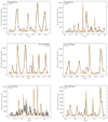 |
Fig. B.1. Mixed-mode pattern for KIC 6847371 ( |
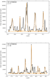 |
Fig. B.2. Same labels as in Fig. B.1 for KIC 6768042 ( |
Pressure dipole mode widths compared to the radial mode widths.
Estimates of the ratio ζ between the mode inertia in the core and the total mode inertia, the mixed dipole mode widths Γn, 1, heights Hn, 1 and the pressure dipole mode widths  for the stars KIC 6847371 at radial order n = 5 and 6, KIC 11032660 at n = 5 and 6, KIC 5461447 at n = 6, KIC 10857623 at n = 7, and KIC 6768042 at n = 7 and 8.
Appendix C: Table available at the CDS with results of pressure mode-fitting
The approach described in Sect. 3 allowed us to thoroughly characterise the pressure modes of 2103 evolved red giants observed by Kepler with Δν ≤ 4.0 μHz. A selection of the seismic parameters, obtained in Sect. 4, is shown in Table C for 25 stars. The complete set of global seismic parameters of the whole sample of stars is available at the CDS. The stellar mass and effective temperature were extracted from the APOKASC catalogue (Pinsonneault et al. 2014). For some stars, the stellar mass and the effective temperature are not listed in the APOKASC catalogue. It concerns roughly 5% of our sample, with half of this fraction being associated with very low Δν-values (i.e., Δν ≤ 0.5 μHz). For these stars, we nevertheless obtained rough estimates of the stellar mass and effective temperature using semi-empirical and empirical scaling relations implying both the frequency at the maximum oscillation power νmax and large frequency separation Δν (Kjeldsen & Bedding 1995; Kallinger et al. 2010; Mosser et al. 2010).
Seismic parameters.
All Tables
Fit of the seismic parameters ε and d0ℓ, and the dimensionless glitch parameters.
Estimates of the ratio ζ between the mode inertia in the core and the total mode inertia, the mixed dipole mode widths Γn, 1, heights Hn, 1 and the pressure dipole mode widths for the stars KIC 6847371 at radial order n = 5 and 6, KIC 11032660 at n = 5 and 6, KIC 5461447 at n = 6, KIC 10857623 at n = 7, and KIC 6768042 at n = 7 and 8.
All Figures
|
Fig. 1. Upper panel: distribution of our sample of stars as a function of Δν, with red giants in blue and He-burning stars in red. Stars with unidentified or uncertain evolutionary stage are plotted in grey. The inset is a zoom-in portion of the large panel. Lower panel: seismic diagram of our sample of stars with the same colour code as in the upper panel, where 1/νmax is a proxy for the luminosity. The solid black line is the evolutionary track of a 1 M⊙ model computed with MESA, using the 1M_pre_ms_to_wd test suite case. Some key events are highlighted: the RGB bump (RGB-b), the luminosity tip of the RGB (RGB-tip), and the AGB bump (AGB-b). |
| In the text | |
|
Fig. 2. Oscillation spectrum of the star KIC 2695975 (Δν = 1.538 μHz, and νmax = 10.11 μHz), with an emphasis on the spectral range where the power spectral density is integrated for each mode. Red, blue, green, and light blue are associated with radial, dipole, quadrupole, and octupole modes, respectively. This star has been classified as an RGB star with the two identification methods adopted in this work. |
| In the text | |
|
Fig. 3. Seismic parameters of the asymptotic pattern of red giants (Eq. (1)) after adjusting Δν with the best-matching template following the procedure described in Sect. 3. Upper left panel: acoustic offset ε as a function of Δν, where blue triangles indicate RGB stars and red diamonds He-burning stars. Stars with either an unidentified evolutionary stage or disagreement between the two classification methods described in Sect. 2 are represented in grey. Upper right panel: reduced small separation d02 as a function of Δν; the stellar mass is colour-coded. Bottom panels: same labels as for the upper right panel, but for d01 and d03 as a function of Δν. The solid blue and red lines are the median values in 0.4 μHz Δν bins for low-mass stars (M ≤ 1.2 M⊙) and for high-mass stars (M ≥ 1.2 M⊙), respectively. The dashed orange lines represent the scaling relations from Mosser et al. (2013a), and the solid dark blue lines are the scaling relations derived in this study (listed in Table 2). The dot-dashed pink and dark green lines correspond to the scaling relations for less evolved stars from Corsaro et al. (2012) and Huber et al. (2010), respectively. Mean error bars estimated at low Δν (Δν ≤ 1.0 μHz) and at high Δν (Δν ≥ 1.0 μHz) are represented at the bottom of each panel. |
| In the text | |
|
Fig. 4. Modulation amplitude 𝒜, modulation period 𝒢, and modulation phase Φ as a function of Δν, with the same labels as in Fig. 3. The thick solid lines are the median values in 0.5 μHz Δν bins, shown in blue for RGB stars and in red for He-burning stars. In the upper panels, dashed blue lines are the fits presented in Table 2. In the upper left panel, the dashed orange line is the fit obtained for less evolved stars (Vrard et al. 2015), corrected with a factor that accounts for the differences between the methods we used to fit the modulation as described in Sect. 4.2. In the upper right panel, dotted black lines delimit the domain of reliable measurements of 𝒢, which are described in Sect. 3, and the thin solid line is the modulation period inferred from MESA models for a 1 M⊙ star and starting from the RGB up to the AGB. The error bars are computed in the same way as in Fig. 3. In the lower right panel, the stellar mass is colour-coded, and medians are represented by solid lines for low-mass stars (M ≤ 1.2 M⊙) and by dashed lines for high-mass stars (M ≥ 1.2 M⊙). Because Φ varies with stellar evolution, we calculated the medians for RGB and He-burning stars separately. We show them in blue for RGB and in red for He-burning stars. |
| In the text | |
|
Fig. 5. Upper panels: ⟨Γ0⟩ as a function of Δν and Teff. Middle panels: ratio of ⟨Γ1⟩ and ⟨Γ0⟩ as a function of Δν and ⟨Γ1⟩ as a function of Teff. For convenience, horizontal dotted black lines are plotted at specific values of 0.5, 1.0, 1.5, and 2.0. Bottom left panel: ⟨Γ2⟩ as a function of Teff. The colours and symbols are the same as in Fig. 4. Mean error bars on the widths have been computed both at low Teff (Teff ≤ 4200 K) and at high Teff (Teff ≥ 4200 K). These limits are equivalent to the limits in Δν chosen in Fig. 3. The fits presented in Table 3 are plotted with dashed light blue lines for RGB stars. Bottom right: ⟨Γ1⟩ as a function of Δν with the dipole mode visibilities colour-coded. The solid and dashed lines correspond to the median values for low-visibility dipole modes ( |
| In the text | |
|
Fig. 6. Radial mode amplitude ⟨A0, bol⟩ computed from Eq. (13) as a function of νmax with the stellar mass colour-coded. The dashed lines are the fits presented in Table 3, shown in blue for low-mass stars (M ≤ 1.2 M⊙) and in red for high-mass stars (M ≥ 1.2 M⊙). The error bars are computed in the same way as in Fig. 5. |
| In the text | |
|
Fig. 7. Upper panels: visibility of the ℓ = 1 modes as a function of Teff in the left panel and of νmax in the right panel. The colours and symbols are the same as in Fig. 5. The error bars are computed in the same way as in Fig. 5. Similarly, error bars on the visibilities are given for both low νmax (νmax ≤ 4.5 μHz) and high νmax (νmax ≥ 4.5 μHz). The dashed lines are the fits presented in Table 4, in light blue for RGB stars and in light red for He-burning stars. The thin solid light blue and light red lines are the fits obtained for less evolved stars (Mosser et al. 2012) for RGB stars and for He-burning stars, respectively. The thin solid black line is the theoretical prediction (Ballot et al. 2011b). Middle panels: same labels as in the upper panels, but for the visibility of ℓ = 2. Lower left panel: same labels as in the upper left panel, but for the visibility of ℓ = 3 modes. The median values are computed in 50 K wide Teff bins and in 1.5 μHz wide νmax bins. |
| In the text | |
|
Fig. 8. Top panel: ratio of the average radial mode widths ⟨Γ0⟩ obtained in this study and those obtained with a Bayesian method (Kallinger 2019). The median values are computed in 0.015 μHz wide Γ0, freq bins. Bottom panel: same as in the upper panel, but for the average radial mode bolometric amplitude ⟨A0, bol⟩. The colours and symbols are the same as in Fig. 4. The median values are computed in 20 ppm A0, freq bins. The dotted line represents the 1:1 agreement. Mean error bars are represented at the top of each panel. |
| In the text | |
|
Fig. 9. Left panel: distribution of He-burning stars in terms of νmax. In blue we show the number of low-mass He-burning stars (M ≤ 1.2 M⊙), and in green we show the number of high-mass He-burning stars (M ≥ 1.2 M⊙). The colour bar indicates the location in νmax where we expect the AGB bump for a given mass following Eq. (19) and adopting Teff = 4800(νmax/40.0)0.06 (Mosser et al. 2010). The blue and green arrows roughly indicate the location of the AGB bump for low-mass and high-mass stars, respectively, which is characterised by a local excess of stars. Right panel: Evolution speed dνmax/dτ, where τ is the stellar age, as a function of νmax for different stellar masses. The models computed with MESA start from the end of the clump phase, which is marked by a diamond. The start and the end of the AGB bump are marked by a circle and a star, respectively. |
| In the text | |
|
Fig. 10. Ratio of the mode visibilities of odd and even degrees as a function of νmax. Same labels as in Fig. 4. For convenience, horizontal dashed black lines are plotted at specific values of 0.75, 1.00, and 1.25. The error bars are computed in the same way as in Fig. 3. The median values are computed in 1.5 μHz νmax bins. |
| In the text | |
|
Fig. B.1. Mixed-mode pattern for KIC 6847371 ( |
| In the text | |
|
Fig. B.2. Same labels as in Fig. B.1 for KIC 6768042 ( |
| In the text | |
Current usage metrics show cumulative count of Article Views (full-text article views including HTML views, PDF and ePub downloads, according to the available data) and Abstracts Views on Vision4Press platform.
Data correspond to usage on the plateform after 2015. The current usage metrics is available 48-96 hours after online publication and is updated daily on week days.
Initial download of the metrics may take a while.