| Issue |
A&A
Volume 697, May 2025
|
|
|---|---|---|
| Article Number | A165 | |
| Number of page(s) | 16 | |
| Section | Stellar structure and evolution | |
| DOI | https://doi.org/10.1051/0004-6361/202452635 | |
| Published online | 16 May 2025 | |
Red giant evolutionary status determination: The complete Kepler catalog
1
Université Côte d’Azur, Observatoire de la Côte d’Azur, CNRS, Laboratoire Lagrange, Bd de l’Observatoire, CS 34229, 06304 Nice Cedex 4, France
2
Department of Astronomy, The Ohio State University, 140 West 18th Avenue, Columbus, OH 43210, USA
3
School of Physics and Astronomy, University of Birmingham, Birmingham B15 2TT, UK
4
Kavli Institute for Astrophysics and Space Research, Massachusetts Institute of Technology, Cambridge, MA 02139, USA
5
Institute for Astrophysics (IfA), University of Vienna, Türkenschanzstrasse 17, 1180 Vienna, Austria
6
Max-Planck-Institut für Sonnensystemforschung, Justus-von-Liebig-Weg 3, 37077 Göttingen, Germany
7
LIRA, Observatoire de Paris, Université PSL, Sorbonne Université, Université Paris Cité, CY Cergy Paris Université, CNRS, 92190 Meudon, France
8
Université Paris-Saclay, Université Paris Cité, CEA, CNRS, AIM, 91191 Gif-sur-Yvette, France
9
Department of Astronomy, University of Florida, Bryant Space Science Center, Stadium Road, Gainesville, FL 32611, USA
10
Institute for Astronomy, University of Hawai’i at Mānoa, 2680 Woodlawn Drive, Honolulu, HI 96822, USA
11
Department of Physics, The Ohio State University, 191 West Woodruff Ave, Columbus, OH 43210, USA
12
Heidelberg Institute for Theoretical Studies, Schloss-Wolfsbrunnenweg 35, 69118 Heidelberg, Germany
13
Zentrum für Astronomie, Landessternwarte (ZAH/LSW), Heidelberg University, Königstuhl 12, 69117 Heidelberg, Germany
14
Instituto de Astrofísica de Canarias (IAC), E-38205 La Laguna, Tenerife, Spain
15
Universidad de La Laguna (ULL), Departamento de Astrofísica, E-38206 La Laguna, Tenerife, Spain
16
School of Physics, University of New South Wales, NSW 2052, Australia
17
Sydney Institute for Astronomy (SIfA), School of Physics, University of Sydney, NSW 2006, Australia
⋆ Corresponding author: mathieu.vrard@oca.eu
Received:
16
October
2024
Accepted:
4
March
2025
Context. Evolved cool stars have three distinct evolutionary status: shell-hydrogen burning (RGB), core-helium and shell-hydrogen burning (RC), and double-shell burning (AGB). Asteroseismology can distinguish between the RC and the other status, but distinguishing RGB and AGB has been difficult seismically and spectroscopically. The precise boundaries of different status in the Hertzprung–Russel (HR) diagram have also been difficult to establish.
Aims. In this article we present a comprehensive catalog of asteroseismic evolutionary status, RGB and RC, for evolved red giants in the Kepler field. To prepare this catalog we carefully examined boundary cases to define the lower edge of the RC phase in radius and surface gravity. We also tested different published asteroseisemic methods claiming to distinguish AGB and RGB stars against a sample where AGB candidates were selected using a spectrocopic identification method.
Methods. We used six different seismic techniques to distinguish RC and RGB stars, and tested two proposed methods for distinguishing between AGB and RGB stars. These status were compared with those inferred from spectroscopy.
Results. We present consensus evolutionary status for 18 784 stars out of the 30 337 red giants present in the Kepler data, including 11 516 stars with APOGEE spectra available. The agreement between seismic and spectroscopic classification is excellent for distinguishing RC stars, agreeing at the 94% level. Most disagreements can be traced to uncertainties in spectroscopic parameters, but some are caused by blends with background stars. We find a sharp lower boundary in surface gravity at log(g) = 2.99 ± 0.01 for the RC and discuss the implications. We demonstrate that asteroseismic tools for distinguishing between AGB and RGB stars are consistent with the spectroscopic evolutionary status at near the RC (with the asteroseismic large separation Δν ≤ 2 μHz), but that the agreement between the different methods decreases rapidly as the star evolves during the AGB phase.
Conclusions. This work presents the most complete evolutionary status catalog for Kepler and APOGEE red giant stars. The data precisely defines the locus of RC stars in the HR diagram, an important constraint for stellar theory and stellar populations. We also demonstrate that asteroseismic tools can distinguish between AGB and RGB stars under some circumstances, which is important for the age estimation of field stars. However, we also put forward the importance of using several techniques to assess the evolutionary status determination for luminous red giants.
Key words: stars: evolution / stars: interiors / stars: low-mass / stars: oscillations / stars: solar-type
© The Authors 2025
 Open Access article, published by EDP Sciences, under the terms of the Creative Commons Attribution License (https://creativecommons.org/licenses/by/4.0), which permits unrestricted use, distribution, and reproduction in any medium, provided the original work is properly cited.
This article is published in open access under the Subscribe to Open model. Subscribe to A&A to support open access publication.
1. Introduction
Luminous red giants are prime targets for modern surveys of Galactic populations and their implications for galaxy formation and evolution. Historically, however, it has proven challenging to infer masses and ages for red giants. The underlying cause is straightforward; stars with a wide range of birth mass and composition converge into a remarkably small range of surface temperature after leaving the main sequence, particularly when they burn their helium in their core. Furthermore, all evolved giants have a wide dynamic range in luminosity. Therefore, both of the classical mass diagnostics on the main sequence (surface temperature and luminosity) are difficult to use as reliable mass or age indicators for cool giants. An important solution to this problem came with the emergence of large-scale asteroseismology. With the launch of the space missions CoRoT (Convection, Rotation and planetary Transits: Baglin et al. 2006) and Kepler (Borucki et al. 2010), we discovered that virtually all cool evolved stars exhibit rich power spectra showing evidence of many oscillation frequencies. Turbulence in the outer layers of giants, which excites waves, is a natural physical explanation. Red giant stars are solar-like oscillators that present mostly pressure modes in their spectra. They are the signature of acoustic waves stochastically excited by turbulent convection in the outer layers of the star. In combination with effective temperatures, the information derived from the radial modes is used to deliver unique information on stellar masses and radii (e.g. Kallinger et al. 2010).
Red giant stars can also be divided into three distinct evolutionary states. First ascent red giants, hereafter RGB stars, have a hydrogen-burning shell surrounding an inert helium core. Once helium ignites in the core, they become red clump (RC) stars, with core He burning and shell-hydrogen burning. Once RC stars exhaust core helium, they become double-shell burning stars (hydrogen and helium), and they asymptotically approach the RGB; we refer to these as asymptotic red giant (AGB) stars. The RC is prominent in field stellar populations, and it is a potent diagnostic of stellar populations and stellar physics. As an example, RC stars are commonly used as distance and extinction indicators (see e.g. Girardi 2016, for a more complete description of the use of RC stars).
However, the spectroscopic parameters of RC stars are very close to RGB and AGB stars, therefore producing a possible confusion between the evolutionary status. If the observed sample of stars spans a large range of metallicity, distances, or ages, the location of the RC overlaps the RGB in the color–magnitude diagram, therefore rendering its identification difficult. In addition, RC and RGB stars have very different internal structures, and RC stars can have experienced significant mass loss relative to RGB stars because they are in a later evolutionary status. Both of these effects can be important for understanding the ages and masses of both stellar populations.
Fortunately, with the advent of asteroseismology it became apparent that RC and RGB stars had different oscillation frequency patterns (Dupret et al. 2009; Mosser et al. 2012b), tied to differences in their internal structure. These pattern differences, as discussed below, can be used to infer asteroseismic evolutionary status that are precise and accurate. (e.g. Bedding et al. 2011; Mosser et al. 2011a). The underlying cause is that red giant oscillation spectra exhibit nonradial mixed modes (Beck et al. 2011) in addition to pure pressure modes. Because they behave as acoustic waves in the envelope and as gravity waves in the core, they carry unique information on the physical conditions inside the stellar cores. Therefore, dipole mixed modes can be used to distinguish RC stars from RGB stars. Several automated methods were developed during the last decade using differences in the mixed mode pattern to separate RC from RGB stars (Stello et al. 2013; Vrard et al. 2016; Elsworth et al. 2017; Hon et al. 2017, 2018). Several other techniques, focusing on the use of the pressure modes, were also developed (Kallinger et al. 2012; Mosser et al. 2019). These methods are supported by evidence that the evolutionary status also has an influence on the pressure mode pattern through the measurement of the helium second ionization zone (Vrard et al. 2015; Dréau et al. 2021) or the solar-like oscillation envelope (Mosser et al. 2012a, 2019). Kallinger et al. (2012) and Mosser et al. (2019) also attempted to distinguish AGB from high-luminosity RGB stars, but without independent verification.
The precise determination of the evolutionary status also recently allowed characterization of the beginning of the RC phase called the zero-age sequence of helium-burning stars (ZAHB). This feature, a robust prediction of stellar structure and evolution theory, was first clearly identified in globular star clusters and quantified in the 1950s (e.g. Arp et al. 1953). However, it was more difficult to observe in field populations until the advent of asteroseismology. With asteroseismic determinations of evolutionary status, a clear boundary on the mass–radius diagram is evident (Li et al. 2021). Stars below the bulk population were identified as peculiar stars showing evidence of mass loss (Li et al. 2022). The precise location in the HR diagram of the ZAHB is a sensitive test of stellar model physics. A good example is core overshooting (Tayar & Pinsonneault 2018). Therefore, measuring the evolutionary status of a larger number of stars will lead to a better understanding of the RC characteristics and the physics occurring during this phase of stellar evolution.
Spectroscopy and precise photometry can also be used to separate out stars in different evolutionary status. This is most clearly seen in star clusters, where the RC and RGB are distinctively separated, with the RC being systematically hotter (Brogaard et al. 2012; Handberg et al. 2017). Core He-burning stars with a wide range of masses and metallicities are found in the RC (Vrard et al. 2016). The temperature offset is a weak function of mass and metallicity (Pinsonneault et al. 2025). At sufficiently low mass or metallicity a blue horizontal branch emerges, and the temperature offset becomes a strong function of mass; however, such stars are typically too hot to show solar-like oscillations. The AGB is more sparsely populated, but is also hotter, and clearly distinct from the RGB in populous globular clusters. Clear examples of this separation can be seen in Figure 3 of the Gaia DR2 release paper (Babusiaux 2018). For those stars it is therefore possible to clearly separate RGB from RC and AGB stars by defining a temperature difference between these populations with composition, mass, and age information. These differences are blurred in field populations, where the RGB locus is a very sensitive function of metallicity, and masses are more challenging to infer using traditional tools.
The APOGEE survey (Majewski et al. 2017; Wilson et al. 2019) used asteroseismic surface gravities as a fundamental calibrator. However, it quickly became apparent that there was an offset between asteroseismic and spectroscopic surface gravities that depends on evolutionary status. This finding implied that it was necessary to infer a spectroscopic evolutionary status for the vast majority of APOGEE targets without asteroseismology in order to ensure that the appropriate correction was applied to the data. The basic principle was as follows. At any given age and composition, there is a clear slope in Teff as a function of log(g) for the RGB in the HR diagram that can be empirically measured. The APOGEE survey provides precise and accurate abundances (Jönsson et al. 2020). For the overlap sample between APOGEE and Kepler, the mass, metallicity, and evolutionary status are all known. The observed properties of the stars can then be used to remove mass and composition effects, producing a temperature offset distribution for field stars that is similar to the star cluster case. When this is done, the temperature offset between the RC and RGB is clearly seen, and can be used as a reliable diagnostic of evolutionary status (Jönsson et al. 2020). This approach was used in APOGEE DR16 (Jönsson et al. 2020), and a related formulation was derived for DR17 (Warfield et al. 2024).
The process just described did not include any attempt to distinguish between RGB and AGB status. However, the same principles can be applied to them as for the RC: there are two clearly separated branches just above the RC in the HR diagram. The main and most important difference is that the AGB and RGB converge at higher luminosity and lower surface gravity compared to the RC, meaning that they are not easy to distinguish in the luminous domain. We discuss our detailed method for separating these groups in Section 8.
Elsworth et al. (2019) used the large number of automated techniques, both asteroseismic and spectroscopic, able to evaluate the evolutionary status of a large number of red giant stars. Good agreement was found between the methods. We believe that it is appropriate to re-address this question for several reasons. First of all, new techniques have been developed since then (Mosser et al. 2019; Kuszlewicz et al. 2020). We also have an extended sample available for analysis called the Kepler Red giant Legacy catalog. This final Kepler red giant data sample, treated specifically for seismology, were recently analyzed (Garcia et al. in preparation). The Kepler seismic sample now contains 30 337 red giants and the APOGEE data release 15 464, while Elsworth et al. (2019) concentrated their analysis on 6661 stars. A larger spectroscopic data set from APOGEE is also available, allowing a thorough study.
In this paper, using the extensive amount of data available, our aim is to compare and assess the reliability of seismic methods to obtain the evolutionary status of red giants (RC or RGB). We then evaluate the agreement with the spectroscopic evolutionary status determination, thereby improving its calibration. Additionally, we analyze what these new evolutionary status results bring to our understanding of stellar evolution and stellar models using seismic and spectroscopic data. For this analysis, we focused on a subsample of stars that have APOGEE data: APOKASC-3 (Pinsonneault et al. 2025). With our large sample, we were also able to perform a search of stars below the traditional location of the RC, to precisely measure the minimum surface gravity for the population. Finally, we discuss the possibility of separating, seismically and spectroscopically, the AGB from the RGB stars beyond the RC.
The layout of the paper is as follows. Section 2 describes the seismic and spectroscopic data and the extraction of the main seismic and spectroscopic stellar parameters. Section 3 introduces the characteristics of the different seismic methods that were used in this work. Section 4 sets out the merging of the methods to obtain the finalized list of stellar evolutionary status and evaluate the agreement between the different methods. Section 5 details how the spectroscopic classification was performed. Section 6 is devoted to the comparison between the results of spectroscopic and seismic classification. Section 7 approaches how the development of such a large sample of stars with identified evolutionary status can be used as observational constraints for models. Section 8 addresses the determination of the evolutionary status beyond the RC phase. Finally, Section 9 is devoted to our conclusions.
2. Selection and description of seismic data
2.1. Kepler observations and data selection
We used the KEPSEISMIC11 long cadence Kepler light curves with a 20-day high-pass filter. Light curves corresponding to stars with a median νmax or with an APOGEE predicted spectroscopic νmax below 15 μHz were recomputed and analyzed using an 80-day high-pass filter. The data were corrected following the methods explained in García et al. (2011) with gaps filled using a multiscale discrete cosine transform (García et al. 2014). The initial seismic sample of stars was obtained from the preparatory work done for the red giant Kepler legacy catalog (García et al., in prep.) containing 30 337 candidate stars. We use the Δν and νmax determined in García et al. (in prep.) using the same techniques described in Pinsonneault et al. (2025) as our preliminary asteroseismic values. They were determined for 25 393 stars (García et al., in prep., see also Table 2 of this article). Although we use the ensemble of these stars for the evolutionary status analysis, we later focus on a subsample of 15 464 stars with APOGEE values from Pinsonneault et al. (2025). For the rest of the paper we call this subsample the APOKASC-3 sample.
2.2. Determination of the global seismic parameters
Pinsonneault et al. (2025) inferred the global asteroseismic properties Δν and νmax for all targets. They used a total of 10 distinct techniques for νmax and 7 for Δν and performed a rejection of outliers and background sources, corresponding here to background stars that are not red giants. Where possible, background sources were identified with the use of the spectroscopic APOGEE data: an estimation of νmax is deduced from spectroscopy, with surface gravities and effective temperatures, and compared to the measured νmax (Pinsonneault et al. 2025). If this measurement is out of the rough domain expected given the spectroscopic data, the value is considered as a background source. An outlier rejection processed was also performed by rejecting measurements discrepant from the median at more than 5σ. Details of the process are described in Pinsonneault et al. (2025) and Garcia et al (in preparation). For stars without APOGEE spectra we required detections in both Δν and νmax from 3 different methods. We then used the median values as an estimation of Δν and νmax, as described in Section 2.1. These estimations were used in the remainder of the article, particularly as an aid by the different evolutionary status determination methods. We note that the global seismic parameters for the stars without APOGEE spectroscopic data are preliminary ones. We present the evolutionary status of these stars in this paper, and defer a more detailed discussion of their properties to Garcia et al. (in prep.).
2.3. APOGEE data description and selection
Our paper uses spectroscopic data obtained with the 2.5-meter Sloan Foundation telescope (Gunn et al. 2006) as a part of the high-resolution APOGEE near-infrared survey (Majewski et al. 2017; Wilson et al. 2019). Spectroscopic parameters were inferred with the ASPCAP pipeline (García Pérez et al. 2016), applying the linelists (Shetrone et al. 2015; Smith et al. 2021) and the calibration procedure described in Jönsson et al. (2020).
We use the sixteenth data release from the Sloan Digital Sky Survey (Ahumada et al. 2020), hereafter DR16. All Kepler field targets were obtained prior to the most recent data release, DR17 (Abdurro’uf et al. 2022), so the DR16 sample is complete. In DR16 a polynomial fit to distinguish spectroscopic evolutionary status was adopted, then the asteroseismic status was applied as a calibration sample (see Section 5 below). This was replaced with a neural net classification in DR17, which is less useful for our purposes, because we need to extend the APOGEE calibration to AGB stars. Our approach uses the published APOGEE parameters, and we do not have access to the neural net used to train the DR17 data. As a consequence, we adopted the Warfield et al. (2024) methodology. We therefore work with the DR16 data for this project; the two releases are calibrated to the same fundamental system and are close to one another in mean properties. See Pinsonneault et al. (2025) for a more detailed comparison.
Our Kepler field data were selected to prioritize targets with time domain data. See Pinsonneault et al. (2014) for a discussion of the Kepler selection function, Zasowski et al. (2017) for APOGEE targeting, and Pinsonneault et al. (2018) for specific targeting data in the Kepler fields.
3. Description of seismic methods
In this section, we briefly describe the different methods that were used to determine the evolutionary status of red giant stars. Most of these methods focus on the separation between RC (He-core-burning objects, including massive stars usually called secondary red-clump stars) and RGB stars because differentiating AGB and high-luminosity RGB stars is particularly challenging. AGB and RGB stars have a similar mode pattern with small Δν and νmax and similar gravity-mode period spacings (ΔΠ1) (Stello et al. 2013, their Figure 4b). Moreover, the increasing lifetime of the mixed modes when the star evolves on the RGB or AGB branch render the detection of those modes particularly difficult with Kepler length of observation; the decreasing coupling to the core with increasing luminosity makes detecting mixed modes even more difficult (Grosjean et al. 2014). Therefore, in this Section we focused on the separation between RC and RGB stars.
3.1. First method (Str): Vrard et al. (2016)
This first method is based on the measurement of the asymptotic gravity-mode period spacing (ΔΠ1), as given by Vrard et al. (2016). The technique is based on the stretching of the frequencies in the oscillation spectrum (Mosser et al. 2015) in order to obtain a mixed-mode pattern spaced regularly in period, corresponding to ΔΠ1.
The radial (ℓ = 0) and quadrupole (ℓ = 2) modes are first identified using the universal red giant oscillation pattern as described by Mosser et al. (2011b) then suppressed from the spectra. Then, the modification of the spectrum frequencies is applied and it follows that the regularity of the g-mode pattern can be measured using a Fourier Transform. This allows the measurement of the ΔΠ1 parameter and, therefore, permit the determination of the stellar evolutionary status.
3.2. Second method (COR): Mosser et al. (2019)
This second method is based on the measurement of the Δν signal present on the autocorrelation of the star’s time-series. The signature of the pressure mode pattern can be retrieved by performing a Fourier Transform of the filtered Fourier spectrum (EACF) around the observed oscillations. This corresponds in this case to an autocorrelation (Mosser & Appourchaux 2009). The obtained EACF signal can therefore be measured and it appears that this signal is notably lower by a factor of 2.5 for RC stars compared to RGB stars at same Δν values. This difference is partly, if not totally, due to the fact that RC pressure modes have shorter lifetimes than RGB ones (Vrard et al. 2018). This behavior can therefore be used to determine the evolutionary status of red giants.
Because this method is not using the mixed modes pattern or the global seismic parameters, Mosser et al. (2019) has also used it to differentiate AGB and RGB stars. At first approximation, for the construction of the determined evolutionary status sample, the stars labeled as AGB by this method were included in the RGB sample.
3.3. Third method (NeuralNet): Hon et al. (2017, 2018)
Method 3 is a machine learning technique based on 1D convolutional neural networks. For each spectrum, the frequency range where the oscillations are present is folded around 3 Δν ± νmax. The program is then trained on labelled data in order to allow it to recognize the features corresponding to RGB or RC power spectra. The clear difference in the mixed mode pattern between RC and RGB stars is likely the main feature that allows that determination (Hon et al. 2017). Finally, the program is used on non-classified red giants. The success rate of the classification was found to be very high, even for stars with low signal-to-noise spectra (Hon et al. 2018).
3.4. Fourth method (ELS): Elsworth et al. (2017)
This method is based on the measurement of the mixed mode period spacing (ΔP) in the region of the acoustic spectrum where the oscillations are visible. The location of the ℓ = 1 mixed modes in the acoustic spectrum is determined using the Universal Pattern (Mosser et al. 2011b). This information is used to exclude the even ℓ modes from the analysis. A threshold level, based on the signal-to-noise in the spectrum, is applied to the regions around the ℓ = 1 mixed modes and the frequency of all the data points above this threshold is noted. Now working in the period domain, a histogram is formed from the difference in period, between each feature and all the other features within about 0.3Δν. Because the ΔΠ1 parameter (and hence ΔP) is much larger for RC stars than it is for RGB stars, the location of the peak in the histogram allows the classification of the evolutionary status. The evolutionary status is therefore determined following the ΔP and νmax values. More information on the precise definitions of ΔP and νmax are given in Elsworth et al. (2017). This method was proven to be effective in its classification for spectra with resolved and not depressed mixed-modes.
3.5. Fifth method (Clumpiness): Kuszlewicz et al. (2020)
This method uses a machine learning technique and is based on the light-curve characteristics, in contrast to the previous ones which use the power spectrum. The algorithm corresponds to a supervised classification algorithm and is based on the principle that several light-curve characteristics (variance, magnitude, signal coherency, normalized number of zero crossing, median of time-series first differences) are slightly different as a function of the stellar evolutionary status. For each star, these characteristics are measured. The program is, then, trained to classified RGB and RC stars based on already classified data. After that, the program is applied on unclassified red giants. If there is less than a 33% chance that a star is RC (respectively, RGB) it will be classified as RGB (respectively RC). According to Kuszlewicz et al. (2020), the false positive rate for this technique is lower than 8%.
3.6. Sixth method (ABBA): Kallinger et al. (2012)
This last method is based on the precise pressure mode pattern. This technique locates the radial (ℓ = 0) modes in each spectrum and deduces from those frequencies the value of the phase shift ε of the central radial mode, ε corresponding to the offset in the linear asymptotic fit to the acoustic modes. At given Δν, this parameter is significantly different for RGB stars compared to the RC stars (Kallinger et al. 2012). This behavior can be related to deviations from the asymptotic relations due to sharp changes in the internal structure of stars (Vrard et al. 2015). The method was proven to be efficient even at low signal-to-noise (Kallinger et al. 2012; Kallinger 2019; Dréau et al. 2021). However, there is some overlapping between ε values at the same Δν for RGB and RC stars (Kallinger et al. 2012), which can lower the confidence of the classification.
Because this method uses only the pressure mode pattern it can be extended to the distinction between AGB and RGB stars. Here, as for COR, the stars labeled as AGB by this method were included in the RGB sample as a first approximation for the construction of the determined evolutionary status sample.
4. Forging a seismic evolutionary status consensus sample
In this section, we describe the different results that were obtained for each of the previously described methods and explain how we selected the final sample containing consensus values on the star’s evolutionary stages. Each method was applied independently to the asteroseismic data of the stars and without prior knowledge of the extracted spectroscopic parameters.
4.1. Result description
The results from the different techniques are shown in Table 1. Concerning Method 1, two different codes were used as described in Vrard et al. (2016). In the rest of the text, the different techniques will be referred as the results from Method Str1 and Str2.
Number of evolutionary status results given by the different seismic methods for the red giant Kepler legacy sample (Garcia et al., in preparation) and the APOKASC-3 (Pinsonneault et al. 2025) stars.
We can see that the machine-learning techniques (NeuralNet, Clumpiness) and the method COR provide the highest number of results. This is understandable, because these automated techniques are based, respectively, on the shape of the spectra, the light-curves parameters and the pressure mode pattern. Those characteristics can indeed be measured or recognized in an easier way than mixed-modes, therefore allowing a determination of the evolutionary status for a larger number of stars. On the contrary, method Str and ELS give a lower number of results, mainly for RC and RGB stars with νmax > 20 μHz because mixed modes disappear for high-luminosity red giants due to lower coupling between the resonant cavity of the two types of modes (see e.g.: Grosjean et al. 2014). The only exception concerns method ABBA, which is also based on the analysis of the pressure mode pattern but gives a result for a limited number of stars. This can be understood by the fact that this technique needs a precise identification of the modes, which is not easy to realize with a high confidence for a large number of stars. The sample of analyzed stars was therefore restricted for this technique.
The automated techniques that gave the most results (COR, NeuralNet and Clumpiness) also have a few stars they identified as RC in their sample and that possess spectroscopic characteristics (Teff and log(g)) that correspond to the lower part of the RGB. These probable misidentifications are all located near the Nyquist frequency for Kepler targets, which can explain the confusion for automated techniques because the spectra become difficult to analyze at those frequencies. We address the case of these stars later in the paper.
4.2. Merging classification results
For each method, the stars were classified into three categories: RGB, RC or undetermined. We used the comparison between the different methods to improve the robustness of the evolutionary status determination as was done by Elsworth et al. (2019). Putting together the classification provided from those methods was made following five different scenarios:
The first scenario happens when at least three methods agrees with each other on the evolutionary status classification and no technique disagrees. In this scenario, some methods may not provide any results, therefore considering the star’s evolutionary status as unclassified. This is not considered as a disagreement between the methods. In that situation, the consensus on the classification is clear and the star can be considered as a RGB or RC star following what the methods agreed on. The classification is considered as being robust.
The second and third scenarios arise when at least three methods agrees with each other but another one disagrees, the other ones giving an undetermined status classification. In that situation, we looked at which method disagrees with the consensus because some methods are probably less reliable than others. For that work, we considered the methods that based their classification on the mixed modes analysis as the most reliable because it is principally this feature present in the oscillation spectra that allows a distinction between RC and RGB stars. The other methods like the ones presented in Kallinger et al. (2012) (ABBA) and Mosser et al. (2019) (COR) present an overlap between the two populations for the classification criterion they considered. Clumpiness (Kuszlewicz et al. 2020) has also a lower success rate, around 92%, than the methods that use mixed modes. Therefore, when the only disagreement comes from the methods COR, Clumpiness or ABBA, we follow the classification from the other methods. However, when the disagreement comes from methods Str1, Str2, NeuralNet or ELS, we classify the star as having an uncertain evolutionary status.
A fourth scenario occurs when two methods or more are giving an evolutionary status determination that contradicts two other methods or more. In that situation, the star is classified as having a conflict in the evolutionary status classification. We discuss these stars in more detail in part Section 4.4.
The last scenario corresponds to when two or fewer methods are giving a classification result. In that situation, we considered that a consensus is not reached on the evolutionary status. Therefore, the star is classified as having an undetermined evolutionary status.
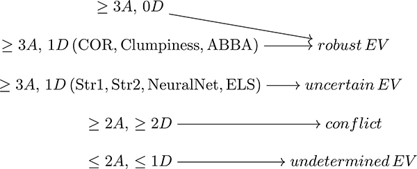
Below is a summary of the classification process for the evolutionary status (here noted EV) as a function of the number of agreements (A) and disagreements (D) between the different methods.
4.3. Classification results and discussion
From this classification, we obtained an evolutionary status for 18784 stars (11387 RGB and 7397 RC). Among them, we have
APOGEE data for 11516 stars (6732 RGB and 4784 RC). The results are displayed in Figure 1 for APOGEE data and the complete results are available at the CDS. The first lines of the data file are given as an example in Table 2. The RC appears in a well defined compact line with 2 < log(g) < 3. However, a few stars, identified by several methods as RC stars, appear to have particularly high and low surface gravity values. We discuss these stars in more detail in Section 7. The RGB (or AGB) are distributed along all the red giant branch except at high and low surface gravity. The low red giant branch is not visible because the detection of seismic oscillations below the Nyquist frequency (corresponding to approximately 283.0 μHz for Kepler long-cadence data) is very difficult and will greatly affect possible consensus on the evolutionary status. The tip of the RGB or AGB is also not visible: the detection of the oscillation for highly luminous RGB and AGB becomes very difficult because of the length of the pulsations and the small number of visible modes (e.g. Mosser et al. 2013; Stello et al. 2014). The length of the observation does not ensure a high enough spectral resolution to obtain an estimation of the seismic parameters, therefore hampering a possible consensus on the evolutionary status for those stars. We note that, above the RC, fewer RGB or AGB stars have an identified evolutionary status. The cause of this comes from the lower number of methods retrieving an answer for these red giants because most of the techniques are using the fine structure of the oscillation spectrum to reach a conclusion on the evolutionary status. Because the characterization of the fine structure of the star’s spectrum is more difficult to perform at lower νmax, it results that the number of stars with confirmed evolutionary states will be lower.
First lines of a joined file summarizing the evolutionary status determination.
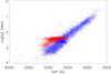 |
Fig. 1. Stellar surface gravity as a function of the effective temperature Teff for the stars classified as having a robust evolutionary status. The red stars represent the RC and the blue stars represent the RGB or AGB stars for high-luminosity targets. |
We also note that a few stars appears to possess values of Teff and log(g) far away from what we expect for red giants. We have a few hundred with Teff and log(g) closer to main-sequence stars than to red giants. This behavior corresponds in part to the fact that the spectroscopic measurement can be biased by the presence of background stars with different Teff and log(g) values (Pinsonneault et al. 2012) and, in part, from the selection of the red giant Kepler legacy sample that contains a few targets wrongly identified as giants because their aperture are polluted by nearby red giants (Garcia et al. in preparation). These targets will be checked and modified in the published version of the red giant Kepler legacy sample. Four stars with very low spectroscopic surface gravity and identified as RC by seismology are also present in the final sample. Those targets are identified as likely belonging to background stars because their spectroscopic log(g) values deviates more than 2 σ from the seismic ones.
The stars with undetermined evolutionary status due to too few results from the different methods are shown in a Kiel diagram in Figure 2. There are 5276 such APOKASC-3 stars (9211 for the full red giant legacy sample). Most of those correspond to stars with very low or very high surface gravity, particularly stars with a νmax value near the Nyquist frequency. This is consistent with the difficulty to obtain a reliable seismic measurement for these stars. We note particularly that many of these stars have Teff and log(g) corresponding to main-sequence or subgiants rather than giants. Those characteristics correspond certainly to blended sources in the Kepler pixels: stars with different Teff and log(g) blended in the same KIC number. The seismic signature we perceive is thus related to the background red giant star and not the main spectroscopic target. Those faint red giants are particularly difficult to analyze, therefore their evolutionary status will not be determined by the different automated techniques, consistent with the results we obtained. In Figure 2, we can see that most of the targets with main-sequence or subgiant spectroscopic characteristics correspond to stars with long light-curves. It is also clear from Figure 2 that we can detect and classify the vast majority of giants with intermediate surface gravities. It demonstrates that even for long light-curves, the classification for low-log(g) stars is not always easy, probably due to the disappearance of the mixed-modes and the decrease of ΔΠ1 towards the RGB values. A few stars with Teff and log(g) consistent with RC are also present in Figure 2. Those red giants are mostly plotted in green, therefore showing they correspond to stars with short light-curves. These targets have thus low signal-to-noise spectra with additionally a lower spectral resolution, which explain why the determination of their evolutionary status is difficult and no consensus was reached from the different methods.
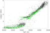 |
Fig. 2. Spectroscopic stellar surface gravity as a function of the effective temperature Teff for the stars having an undetermined evolutionary status (5276 APOKASC-3 targets) and a duration of observation higher than 4 months (3670 APOKASC-3 targets, in black). The green dots correspond to the stars that have a length of observation equal to or lower than 3 months. |
Among the difficulties to measure an evolutionary status, it is well-known that the classification of massive stars is more complicated because of their similarities in their ΔΠ1 values between the RGB and RC phases (Stello et al. 2013; Crawford et al. 2024). In our final APOKASC-3 sample, we have 293 stars with M > 2.4 M⊙, only 67 of them have a mass > 3.0 M⊙. The methods that delivered the most results for M > 2.4 M⊙ targets are COR (for 288 stars), NeuralNet (for 290 stars) and Clumpiness (for 286 stars). Among those methods, only NeuralNet is based in part on the mixed-mode pattern to classify the stellar evolutionary status, however this classification method was shown to be effective even for massive RC targets (Hon et al. 2018). The methods based on the mixed-mode pattern, Str and ELS, delivered fewer results (61 and 124, respectively, for the two Str codes and 186 for ELS). The evolutionary state determination for massive stars is thus driven by methods that are not based on the mixed-mode analysis. Therefore, if the ΔΠ1 values are similar for the two evolutionary status concerning massive stars, it has little influence on the final determination. We also note that, for M > 2.4 M⊙ stars with a large frequency separation coherent with a secondary RC star (typically 4 μHz < Δν < 9 μHz), we have 166 classified as RC, while only 6 as RGB. This is coherent with previous results showing that most massive stars around those Δν values are RC (Crawford et al. 2024). Lastly, we point out that the sample of RGB massive stars corresponds mostly to very low Δν targets. Out of those RGB, we have 90 stars with Δν < 3 μHz among the 118 with M > 2.4 M⊙. The higher number of massive RGB/AGB stars at that stage is probably due to the increasing difficulty of measuring global asteroseismic parameters with decreasing Δν as well as the presence of more massive AGB stars.
Another difficulty can arise with the presence of stars with depressed ℓ = 1 modes (Mosser et al. 2012a). In order to investigate how our evolutionary status determination perform with those targets, we first selected the star sample of Stello et al. (2016). We applied their cut in ℓ = 1 mode visibilities in order to select the stars with depressed ℓ = 1 modes, resulting in 566 stars. Out of those, an evolutionary status was determined for 509 stars. The methods that gave the most results are COR (for 508 stars), NeuralNet (for 503 stars) and Clumpiness (for 501 stars). Here also, only NeuralNet is based in part on the mixed-mode pattern in order to give a classification, showing that it is not the mixed modes that drives the evolutionary status determination for those stars. The two codes we used for Str gave only a classification for few stars: 62 and 8, respectively. However, the ELS method was showing a classification for 448 stars. Nonetheless, even with those results, most evolutionary status determinations are confirmed by the other methods.
In order to evaluate the validity of the evolutionary status classification, we used the sample of stars with depressed ℓ = 1 modes and confirmed evolutionary status analyzed by Mosser et al. (2017). Out of the initial sample of 71 stars, 65 of them have a confirmed evolutionary status in our work. Here also, the methods that participated the most to the determination of the evolutionary status were COR, NeuralNet and Clumpiness, furnishing an answer for the whole 65 targets. However, the other methods reached also a conclusion on the evolutionary status for the majority of the sample: 63 for ELS, 40 and 34 respectively for the two codes that were used for Str. This can be explained by the fact the selected sample possess a mixed-mode pattern in their oscillation spectra clear enough to measure a ΔΠ1, therefore allowing the methods based on the mixed-mode analysis to reach a conclusion even if with depressed ℓ = 1 modes. It is important to note that all evolutionary statuses that we determined with our work are consistent with the ones present in Mosser et al. (2017). With these results, we can say that the evolutionary status determination we performed is reliable for stars with depressed ℓ = 1 mixed modes, mainly because it is driven, in those cases, by methods that are not based on the mixed-mode pattern analysis.
4.4. Conflicted evolutionary status
Among the stars that were not classified as RC or RGB, only 452 of APOKASC-3 red giants have an evolutionary status that corresponds to the fourth scenario when a clear conflict arises between the different methods (650 in the total red giant legacy sample). In order to understand where this conflict arises, we performed a thorough analysis of the evolutionary status of this sample. We checked individually the ΔΠ1 values of those stars following the method of Mosser et al. (2014) and Vrard et al. (2016). We confirmed an unambiguous measurement for 109 stars in this sample. The results are displayed in Table 3. The fraction of stars with disagreements between methods on the evolutionary status is 2.5 − 4.2%, thus showing high level of agreement between the methods. It is important to note that very few (< 10) of these possess short light-curves (< 4 months). Therefore, a determination of the evolutionary status should be possible in those targets.
Stars for which a conflict is present between the different evolutionary status that was given by the different seismic methods.
We can see in Table 3 that the correct evolutionary status for conflict stars, following the checked ΔΠ1 measurement, is deduced correctly for more than 70 % of red giants for Str1, Str2 and ELS. This is consistent with the fact that those techniques based on the mixed modes are more reliable and we confirm our selection of those techniques as more reliable when a conflict is arising. We can note also the good reliability of NeuralNet, which tends to agree with the verified ΔΠ1 values for more than half of the case. This result can be understood because this method is based on the shape of the oscillation spectra around the pure pressure ℓ = 1 modes, therefore on the mixed-mode pattern global appearance. COR, Clumpiness and ABBA show less reliability. Because those techniques are based on secondary indicators or parameters (pressure-mode pattern, light-curve analysis, amplitude of the oscillation envelope) for which the two evolutionary status overlap, this behavior is not surprising. These results highlights the reliability of the mixed-mode based methods when a conflict arises. These results confirm our overall classification approach (Section 4.2), where we adopted the consensus value if a single method disagreed.
For the rest of the analysis, we now focus on the susbsample containing the APOKASC-3 data in the red giant Kepler legacy sample, therefore allowing to perform a more detailed analysis of this sample and its evolutionary status determination.
5. Distinguishing RC and RGB stars with spectroscopic data
The APOGEE survey uses a multilayered approach for measuring stellar properties. In the first set of stages, an automated pipeline is used to infer trial values for key observables (Teff, log(g), the ratios of metals, carbon and nitrogen: respectively [C/M] and [N/M], and the alpha to iron ratio: [α/Fe]). These trial values are then placed on an absolute system in a post-processing calibration step. The assignment of a spectroscopic evolutionary status is an important ingredient for inferring spectroscopic surface gravities because of a still poorly-understood phenomenon: the difference between the trial log(g) (here ginit) and calibrated log(g) (here gcal) is observed to be a function of evolutionary status.
We adopt here the same algorithm for assigning spectroscopic evolutionary states as the one used by the APOGEE survey in DR16 (Jönsson et al. 2020). A related expression, for DR17, can be found in Warfield et al. (2024), which we use here. Spectroscopic evolutionary status take advantage of the fact that the RC exists only in a narrow log(g) range, and that RC stars are hotter than first ascent RGB stars on average. The Teff difference between them, of order 200K, is found to have a weak dependence with mass, metallicity, and surface gravity, although the absolute effective temperatures of both populations are sensitive to all three. The APOGEE survey therefore defines a reference surface temperature (Tref) as a function of log(g), metallicity, and carbon-to-nitrogen: [C/N] (a spectroscopic proxy for mass),
![$$ \begin{aligned} T_{\rm ref} = 3032.8 + 552.6\mathrm{log}(g_{\rm init}) -488.9\mathrm{[M/H]} -357.1\mathrm{[C/N]}. \end{aligned} $$](/articles/aa/full_html/2025/05/aa52635-24/aa52635-24-eq1.gif)
These calculated Tref are the ones being used in the rest of the article. Stars with 3.5 > log(ginit) > 2.38 and Teff > Tref were classified as RC stars in DR16 (Jönsson et al. 2020), and they were assigned a surface gravity

All other stars with log(ginit) < 3.5 had the RGB correction applied,
![$$ \begin{aligned} \mathrm{log}(g_{\rm cal})&= \mathrm{log}(g_{\rm init}) - (-0.441 + 0.759 \mathrm{log}(g_{\rm init}) - \nonumber \\&0.267 (\mathrm{log}(g_{\rm init}))^2 + 0.028 (\mathrm{log}(g_{\rm init}))^3 + 0.135[M/H]) , \end{aligned} $$](/articles/aa/full_html/2025/05/aa52635-24/aa52635-24-eq3.gif)
while dwarfs with log(ginit) > 4 had the following correction applied:
![$$ \begin{aligned} \mathrm{log}(g_{\rm cal}) = \mathrm{log}(g_{\rm init}) - (-0.947 + \frac{{T_{\rm eff}}_{\mathrm{spec}}}{5302} + 0.410\mathrm{[M/H]}). \end{aligned} $$](/articles/aa/full_html/2025/05/aa52635-24/aa52635-24-eq4.gif)
Subgiants with 3.5 < log(g) < 4.0 had a weighted average of the dwarf and RGB values assigned. These surface gravity assignments are important for what follows, because stars with an erroneous spectroscopic evolutionary status will have the wrong correction applied, which moves them away from their true position in the surface gravity-temperature plane. Figure 3 shows the stars asteroseismically classified as RGB (blue) and RC (red) clearly separated in the Tref plane. The large majority of stars fall naturally on the positive side or the negative side of Tref, but a significant subset do not. Those red giants will likely be spectroscopically classified incorrectly relative to the seismic classification. We fitted a Gaussian function over the two evolutionary status samples and found that the width at half maximum of each sample correspond to 44.04 ± 0.43K for RGB and 43.28 ± 0.47K for RC. Because the position at the center of the peak of each sample is −79.46 ± 0.43K for RGB and 82.31 ± 0.47K for RC, the two evolutionary statuses will overlap at less than two times the width at half-maximum of their Tref distribution. The overlap between the two samples, which will produce a misidentification of the evolutionary status, will therefore correspond to more than 5% of the total sample. Here, it corresponds to 5.6% of the stars in our sample. These cases will be discussed in Section 6.2. Other approaches, using more detailed information from the full spectrum, have also been performed (see Ness et al. 2015; Hawkins et al. 2018; Banks et al. 2023, 2024). As seen in Figure 3, the agreement between spectroscopic and asteroseismic states is extremely good even without the usage of full spectral information. We therefore proceed with the APOGEE approach for the remainder of the paper.
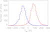 |
Fig. 3. Distribution of stars as a function of Tref. The blue and red histograms correspond respectively to RGB/AGB and RC stars, as determined by seismology following Section 4. |
6. Seismic and spectroscopic evolutionary status comparison
In the APOKASC-3 sample, the seismic evolutionary status is determined for 11371 stars (4755 identified as RC and 6616 identified as RGB or AGB) out of 15 464 red giants, while the spectroscopic evolutionary status was determined for 15 232 stars. Because the seismic and spectroscopic evolutionary status are not obtained uniformly for the whole sample, we focus in this section on the 11 297 stars for which both seismic and spectroscopic classification give an evolutionary status classification.
6.1. Agreement between seismic and spectroscopic classification
In this sample, an agreement between the two evolutionary status determination techniques was found for 10 780 red giants (4530 RC and 6250 RGB or AGB stars), thus 94.80% of the stars where both evolutionary status determination techniques gave a result. This highlights the agreement between the different methods and the accurate calibration of the spectroscopic evolutionary status determination technique as stated by Elsworth et al. (2019). On the contrary, 517 red giants have divergent evolutionary status results. A discussion about these stars is present in Section (6.2).
The results, for the stars where the evolutionary states agree, can be seen on Figure 4. The RC is well defined and separated from the RGB and AGB stars. The secondary clump appears also very clearly and no sample of stars appears to deviate significantly from what is expected for clump and RGB stars.
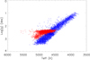 |
Fig. 4. Stellar surface gravity as a function of the effective temperature Teff for the stars showing agreement between the spectroscopic and seismic evolutionary status classification. The red stars represent the RC and the blue stars represent the RGB or AGB stars for high-luminosity objects. |
6.2. Stars with a divergent evolutionary status classification
Divergent evolutionary status between spectroscopic and seismic techniques are present for 517 stars. 215 stars are identified as RC by seismology and as RGB by spectroscopy. On the contrary, 302 stars are recognized as RGB by seismology and as RC by spectroscopy. Their positions in the HR diagram are shown on the top part of Figure 5. These stars are concentrated near the RC because this is the domain where the two populations overlap. The only exceptions concern 4 stars for which the low spectroscopic surface gravity (around 1) does not correspond to the seismic ones which are way higher (between 2.39 and 2.5 for those red giants). These inconsistencies can explain the misidentification of those stars as belonging to the RGB or AGB by the spectroscopic classification. A more thorough discussion on the discrepancies between spectroscopic and seismic log(g) is present in Section 7.
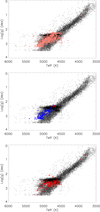 |
Fig. 5. Stellar surface gravity as a function of the effective temperature Teff for the stars with an agreement between the spectroscopic and seismic evolutionary status classification (in black). Top: Stars with divergent spectroscopic and seismic evolutionary status (pink triangles). Center: Stars identified as RGB by seismology and RC by spectroscopy for which the evolutionary status was confirmed as RGB (blue triangles) or RC (red triangles). Bottom: Same as center panel, but the red triangles correspond to confirmed RC stars identified as RC by seismology and RGB by spectroscopy. |
To confirm the evolutionary status of each star with conflict between the seismic and spectroscopic classifications, a specific check of the mixed modes was performed. The evolutionary status was considered to be certain when the measurement of ΔΠ1 following the method of Mosser et al. (2014) and Vrard et al. (2016) was possible. The stars with Δν > 10 μHz were also automatically identified as RGB following the results of Stello et al. (2013) and Mosser et al. (2014). The center and bottom part of Figure 5 show the precise results for the stars with confirmed evolutionary status.
The stars identified as RC by seismology and RGB by spectroscopy was confirmed to belong to the RC for 143 stars out of 215. None were identified as RGB stars. We can see on the bottom part of Figure 5 that a significant part of these stars correspond to secondary clump stars and the high surface gravity RC stars previously identified. Because of their high log(g) values, these stars have higher chances to be classified as RGB by the spectroscopic classification method. A further discussion about these stars is present in Section 7.
The stars identified as RGB by seismology and RC by spectroscopy were confirmed to belong to the RGB for 145 red giants and to the RC for 8 out of 302. The stars identified as true RGB correspond mostly to high-mass stars (83 stars out of 145 have a mass larger than 1.5 M⊙) that are spectroscopically confused as RC because of their high Teff and mass, putting them closer to secondary-clump in the Teff-log(g) space. In this configuration, The [C/N] ratio becomes insensitive to mass for higher mass stars (Roberts et al. 2024), so this is not surprising. The stars identified as true RC have, except for two of them, low values of ΔΠ1 and Δν, meaning they are on their way towards the AGB phase (Stello et al. 2013; Mosser et al. 2014). Their lower seismic parameters certainly explain why several seismic methods identified those stars as belonging to the RGB or the AGB. However, because the ΔΠ1 of these stars is still much higher than those of RGB at the same Δν, they are still in the helium-core-burning phase.
7. Evolutionary status of specific populations and RC lower limit
Figures 1, 4 and the bottom part of Fig. 5 show several RC stars with surface gravities much higher than expected for true RC stars. We checked that the spectroscopic surface gravity is consistent with the asteroseismic one. The seismic surface gravity (g) was obtained through the scaling relation (e.g. Kjeldsen & Bedding 1995):
The spectroscopic and seismic comparison shows an overall good agreement (top part of Figure 6). However, it can be clearly seen that spectroscopic results gives log(g) values up to 3.2, while asteroseismic results stop just below 3. The discrepancies concern a few stars for which their spectroscopic values were overestimated compared to the seismic ones. This is in part due to an incorrect spectroscopic evolutionary status, as can be seen by the blue stars on the top part of Figure 6, which in turn caused the wrong surface gravity correction to be applied. The discrepancies between the two sets of values is apparent in the bottom part of Figure 6 showing a distinct RC edge at log(g) = 2.99 ± 0.01 for seismic results, on the contrary to spectroscopic measurements. This observed strong RC edge is consistent with previous models of secondary clump stars (Paxton et al. 2011; Tayar & Pinsonneault 2018) and can serve as an observational constraint for future stellar evolution models.
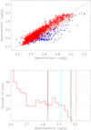 |
Fig. 6. Top: Seismic surface gravity (g) for the stars identified by seismology as belonging to the RC (in red) as a function of the spectroscopic surface gravity. The blue points correspond to the stars identified as RGB by spectroscopy on the contrary to seismic results. Bottom: Seismic surface gravity for the same sample of seismic RC stars, focused on the bottom of the RC. The dashed lines correspond to the maximum values for secondary clump YREC models, with a core overshoot of 0.2 pressure scale height: dark red, cyan, dark green, and pink correspond respectively to stellar models with masses of 3.0, 2.8, 2.6, and 2.4 M⊙. |
In order to assess the possibilities to constrain models for such a clear limit of the secondary RC, we compare those results with models that were computed with the Yale Rotating Evolution Code (YREC, Pinsonneault et al. 1989; van Saders & Pinsonneault 2012). The details of the models are present in Section 2.2 of Tayar & Pinsonneault (2018). Several evolutionary tracks were computed with 4 different masses (2.4 M⊙, 2.6 M⊙, 2.8 M⊙, 3.0 M⊙) and 3 different values of core overshooting (overshoot parameters of 0.0, 0.1 and 0.2 pressure scale heights). Lower masses were not considered because of the difficulty of going beyond the helium flash. The log(g) RC higher limit for the different models with highest overshooting value is shown on the bottom part of Figure 6 and their minimum RC radius for each mass is depicted on Figure 7.
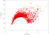 |
Fig. 7. Seismic radius as a function of seismic mass for stars identified as RC following Section 4. The maximum log(g) values of the RC for the different YREC models are represented by the diamonds. The colors depict models with different core overshooting values: no overshooting (dark green), 0.1 pressure scale height (cyan), and 0.2 pressure scale height (dark blue). The minimum radius values for the different MIST tracks are shown as black crosses. |
From those figures, it is clear that models without core overshooting or with low overshooting can not reproduce the observed results on the helium core mass. This conclusion was also reached previously to reproduce ΔΠ1 values by models for RC stars (Bossini et al. 2015; Constantino et al. 2015; Bossini et al. 2017). These previous works, showed that high core overshoot was necessary during the RC phase to match the observations. Here, it is only the model with the most amount of core overshooting until the beginning of the RC phase that can reach the base of the secondary clump in terms of log(g). Having such a hard limit for these RC stars can therefore bring important constraints on stellar models.
Finally, in order to characterize the limits of the clump, we computed the asteroseismic mass and radius of the stars following the seismic scaling relations (e.g. Kjeldsen & Bedding 1995). We used the relations present in the Equation 3 and 4 of Pinsonneault et al. (2018) with solar values present in Table 1 of that same work. We can see in Figure 7 the sharp limit of the zero-age sequence of helium-burning stars (ZAHB) as pointed out by Li et al. (2021) and Li et al. (2022). The presence of this sharp feature is also a confirmation of the robustness of the evolutionary status determination; the small number of stars with lower radius values compared to their masses is indeed consistent with previous results (Li et al. 2022). To compare the position in radius of the ZAHB to theoretical prediction, we used the MESA Isochrones and Stellar Tracks (MIST: Dotter 2016; Choi et al. 2016) based on the MESA models (Paxton et al. 2011, 2013, 2015, 2018). We obtained tracks with masses between 0.8 M⊙ and 3 M⊙, solar metallicity and no extinction. In the MIST models, diffusive overshoot is included in their core and their envelope with an efficiency of fov, core = 0.0160 and fov, env = 0.0174 (Choi et al. 2016; Herwig 2000) The lower radius value during the He-burning phase are represented by black crosses in Figure 7 and reproduce well the global shape of the ZAHB. This curve shape is due to several phenomena, the main one being that low-mass stars (M ≲ 1.8 M⊙) start their helium-burning phase with a degenerate core, therefore with the same He core mass (Girardi 1999; Montalbán et al. 2013). The star with lower masses will then produce the same observed luminosity (Lagarde et al. 2016), therefore reach lower radius. For more massive stars, the He-burning starts in a nondegenerate core leading to lower helium core masses and radii (Girardi 1999; Montalbán et al. 2013), thus producing the observed curved shape. Although the MIST tracks reproduce the global shape of the ZAHB, they do not reproduce the shape in detail. This could be because the full sample has a range of metallicities, and we have shown only the solar metallicity results and one type of overshooting. In order to test the influence on metallicity on the ZAHB shape, we restricted the mass and radius determination to stars with similar metallicities. It appears that it does not have an effect on the lower limit of the ZAHB. Therefore, only the difference in physical processes in the models can explain the differences between the observed ZAHB lower limit and the MIST models. We can also see that the MIST tracks are in agreement with the YREC models with no overshooting, which is surprising because overshooting has been implemented in MIST tracks (Choi et al. 2016; Tayar et al. 2022). However, several other parameters have an influence on the models parameters for red giant stars, the main ones being the description of convective processes at the convective boundaries, the rate of specific nuclear reactions and mass loss at the tip of the RGB (see, for a complete review, Girardi 2016). A global comparison between theoretical models would be necessary to fully understand which parameters affect the differences between the models for massive stars, but is beyond the scope of this paper. Nonetheless, this analysis between theoretical models and observations shows that these results can be used to study the physics of RC models.
8. Asymptotic giant branch stars classification
8.1. Comparison between different asteroseismic methods for the identification of AGB stars
The separation between RGB and AGB stars is difficult to perform with spectroscopy or seismology because the stellar properties of those red giants are very similar. However, two seismic techniques have claimed to be able to disentangle the two evolutionary states using the pressure mode pattern of the star oscillation spectra. Each of them expanded a technique that was tested and calibrated on the separation of RGB and RC stars. ABBA is based on the variation of the pressure mode frequencies as a function of frequency due to discontinuities present in the star’s envelope while COR is based on the amplitude of the envelope autocorrelation function (EACF) used to measure the large separation Δν. The use of those two techniques simultaneously would therefore allow the separation between AGB and RGB stars with more certainty. However, Dréau et al. (2021) observed that the agreement between those two techniques is present at high Δν and νmax but lowers quickly when the star evolves along the AGB or the upper part of the RGB. They found 35% disagreement between the two techniques for stars with Δν ≤ 1 μHz. Because the beginning of the AGB phase starts with a Δν ∼ 2.5 μHz for a typical 1 M⊙ star, this discrepancy appears to rise rapidly. We, thus, need a new method to confirm that we can seismically disentangle the two evolutionary statuses.
With the current data set we possess, there are 76 stars identified as AGB by ABBA for which an evolutionary status is also given by COR. Between those two techniques, we only have a 48.7% agreement, which correspond to a random distribution, therefore pointing toward a lack of agreement between the two methods. However, most of the stars for which the disagreement occurs have very low Δν. Although the stars with Δν ≤ 1 μHz show a systematic disagreement, the agreement fraction increases towards larger Δν, reaching 63.3% for stars with Δν > 1.5 μHz. However, this number is less than two standard deviations away from a random distribution for the star’s identification. The small number of stars in that sample can explain why we have a discrepancy with previous results. It follows that, even if these results seems to be in poor agreement with the previous work of Dréau et al. (2021), we can not reach definitive conclusions about the efficiency of the methods from them. These disagreements confirms previous results that highlighted the need of an independent determination of the evolutionary status for high-luminosity giants, as stated in the previous paragraph.
8.2. Spectroscopic classification of AGB stars
By contrast, spectroscopy can be a useful discriminant between AGB and RGB in some cases. In much the same way as the stars on the RC are hotter than those on the RGB, we expect stars on the AGB to be hotter than those on the RGB at the same mass, metallicity, and surface gravity. AGB stars should also only be present above the luminosity of the RC. In order to have an independent analysis, we perform a spectroscopic determination of the evolutionary status of low surface gravity (log(g) < 2.2) using APOGEE data and evolutionary tracks. For the same reasons stated in Section 2.3, we used the DR16 data for the following part. For each star in the APOKASC-3 sample, an interpolation with the model grid described by Tayar et al. (2017) is performed using the seismic mass, metallicity, [M/H], alpha elements abundance ([α/M]) and seismic log(g). The Teff that the interpolated model possess for each star, named afterwards Tint, is then taken as a reference effective temperature. Tint serves a similar purpose to the Tref, except we actually have the mass of the star, so we can compute the offset from the expected giant branch exactly. The measured offsets between the observed temperature Teff and the model-predicted temperature Tint, we call here ΔTref, were plotted as a function of metallicity in Figure 8. Similar to the results of Tayar et al. (2017), a trend between the temperature offsets and the stellar metallicity can be seen for stars with [Fe/H] < 0.0. For this work, such a trend is not of scientific interest and so we define a function to remove this trend given the stellar metallicity, with the offset being 140K if [Fe/H] ≥ 0.0 and 190[Fe/H] + 140K if [Fe/H] < 0.0. We note that there have been suggestions that the trend should also be a function of alpha abundance (Salaris et al. 2018), mass (Joyce & Chaboyer 2018), surface gravity (Bonaca et al. 2012) and so forth (see Joyce & Tayar (2023) for a more complete discussion). However, we do not explore such complexities here, opting instead for a more simple fit to propose the technique, and expecting later authors to improve upon our results.
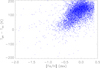 |
Fig. 8. Difference between the star Teff and the reference model effective temperature Tint as a function of metallicity. The Teff and metallicity values are from the APOKASC-3 sample. |
ΔTref is thus obtained with the following relation:
![$$ \begin{aligned} \Delta T_{\rm ref} = T_{\rm eff} - T_{\rm int} -190\mathrm{[Fe/H]} -140, \end{aligned} $$](/articles/aa/full_html/2025/05/aa52635-24/aa52635-24-eq6.gif)
for stars with [Fe/H] < 0.0, and

for stars with [Fe/H] > 0.0. ΔTref should therefore correspond to how much the effective temperature of the star diverges from model predictions, corrected for a metallicity dependent Teff offset in the models. The stars that show a deviation towards high effective temperature, accounting for the uncertainties on Teff, should correspond to the AGB candidates. The ΔTref distribution can be seen in Figure 9 where a clear asymmetry is present towards high ΔTref values, therefore corresponding to hotter stars than predicted by the modeled Tint. This feature in the distribution is a signature of the presence of AGB targets. We decided to take the separation between RGB stars and AGB candidates at 2σ from the original RGB stars distribution as described in Section 5. We also note that the Tref distribution is not exactly centered on 0. In order to take this bias into account, we selected α-rich stars in our sample of low log(g) targets. For these stars, there is a well-defined median mass at a given metallicity, which allows us to better separate the AGB and RGB stars in the HR diagram (Pinsonneault et al. 2025). We fitted the α-rich RGB targets Tref distribution with a Gaussian and found a zero reference point of −26.40 ± 1.25 K. We then used this value as the mean of the original RGB gaussian distribution and select the AGB candidates at 2-σ from the original RGB distribution. The separation between RGB and AGB candidates is shown by the orange dashed line in Figure 9 at Tref = 61.68 K. 398 stars are identified as likely belonging to the AGB following this criterion. We would expect 96 of them to be RGB stars scattered into the AGB domain by observational errors. When the updated DR17 values are used, the exact temperature cutoffs used do shift, but in general the process and the stars identified as potential AGB candidates remain similar.
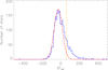 |
Fig. 9. Distribution of stars identified as RGB or AGB, with log(g) < 2.2 (stars above the main RC population in a Kiel diagram) as a function of ΔTref (in blue). The dot-dashed red line shows a Gaussian fit of width 44.04 K centered on −26.40 following the distribution of α-rich stars. The orange dashed line indicates the two-σ limit of the measured RGB sample distribution following Section 5. |
We note that, for the spectroscopic AGB candidates, the offset from the RGB locus tends to be slightly clearer before the metallicity-dependent offset is removed, suggesting that these stars might have metallicity-dependent model offsets that are different from the RGB stars. We also note that there are no obvious chemical differences between our spectroscopic AGB candidates and the RGB stars nearby (e.g. in carbon or oxygen), although we do not necessarily expect any such trends below the AGB bump (Stancliffe et al. 2005; Cinquegrana et al. 2022), and we have not done an exhaustive search for more subtle signals. Some of these stars have low mass, which could indicate mass loss in previous phases of evolution.
8.3. Spectroscopic selection of identified RGB stars
In this work, we also wanted to select stars for which the RGB evolutionary status was certain. In order to achieve that, we used the MIST models previously mentioned in Section 7 and computed the Teff difference between the AGB and RGB tracks at the same log(g). This Teff offset from RGB models rapidly decreases when we reach low log(g) as can be seen in the top panel of Figure 10 for the 1.7 M⊙ MIST evolutionary track and in the other panels of that figure for the 1.0 M⊙ MIST evolutionary track. The rapidity of the decrease highly depends on the model’s mass, being stronger for higher mass stars. In order to be sure to select practically exclusively RGB stars, we took as a reference the 1.7 MIST evolutionary track because its Teff offset value is lower than for lower-mass evolutionary tracks and only few targets have a higher mass in this part of the HR diagram for our stellar sample. We selected stars more than 2-σ away from that track following the original clump star distribution we measured in Section 5. The stars not selected as AGB candidates or RGB are considered as having an undetermined status: RGB/AGB. The classification of the stars (RGB, candidate AGB and AGB/RGB) can be retrieved in Pinsonneault et al. (2025). It is also present in an adjoining file for which the first lines can be seen in Table 4.
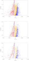 |
Fig. 10. log(g) as a function of ΔTref for the stars above the main RC population. The blue points correspond to the stars identified as RGB targets, the orange points represent stars where the evolutionary status is uncertain, and the red points are AGB candidates. The overplotted solid red and blue lines show the AGB-RGB Teff offset for, respectively, the 1.7 M⊙ and 1.0 M⊙ MIST evolutionary track. Top: full APOKASC-3 sample. Middle: α-poor targets. Bottom: α-rich targets. |
First lines of a joined file summarizing the AGB or RGB evolutionary status determination.
In Figure 10 we show the ΔTref distribution for α-poor (middle panel) and α-rich stars (bottom panel) exclusively. Because the α-rich stars are targets with similar ages and metallicity, we expect them to show a clear difference of ΔTref between their AGB and RGB phases. In the bottom part of Figure 10 we can indeed see a separation between a group of stars near ΔTref = 0, corresponding to RGB targets, and a group of stars with higher ΔTref. This separation is mainly visible for stars with log(g) > 2.0. The group of stars with high ΔTref values corresponds to the MIST 1.0 M⊙ and 1.7 M⊙ AGB evolutionary track and can therefore easily be identified with AGB targets. We can also point out that the AGB selection we performed corresponds to the observed separation between the two groups of stars, therefore confirming that our spectroscopic AGB determination is consistent. In the middle panel of Figure 10 (α-poor stars) we can also note the absence of the hottest stars present in the other panels. They correspond to old low-mass α-rich targets and have likely suffered heavy mass loss during the RGB phase (Miglio et al. 2012, 2021; Howell et al. 2022, 2024, 2025; Pinsonneault et al. 2025). We also plotted the identified AGB and RGB targets in the HR diagram (Figure 11). In this configuration, the separation between AGB and RGB targets is less clear. However we can see that the colder the star at similar log(g), the more likely it is identified as belonging to the RGB, and the hotter the star at similar log(g), the more likely it is identified as belonging to the AGB. It shows also that the hottest stars at same log(g) correspond to the α-rich targets and are all identified as belonging to the AGB.
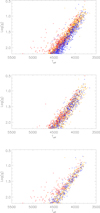 |
Fig. 11. log(g) as a function of Teff for the stars above the main RC population. The blue points correspond to the stars identified as RGB targets, the orange points represent stars where the evolutionary status is uncertain, and the red points are AGB candidates. Top: full APOKASC-3 sample. Middle: α-poor targets. Bottom: α-rich targets. |
8.4. Agreement evaluation between the asteroseismic and spectrocopic AGB determination
Within this spectroscopic AGB candidate star sample, we identified 104 stars for which an evolutionary status is determined with the seismic method ABBA. Among those, 52.0% are in agreement with the spectroscopic identification of AGB targets. Concerning the method COR, 266 stars correspond to the AGB candidate spectroscopic sample. 37.2% are in agreement with the AGB candidates identified by our spectroscopic determination. The agreement between the spectroscopic and seismic results are particularly low and can correspond to a random identification, even if we consider that the number of false positive determination of AGB targets is nonnegligible and that the number of AGB is expected to be significantly lower compared to RGB targets (Karakas et al. 2022).
In order to investigate this behavior, we plot in Figure 12 the agreement between the spectroscopic and the seismic methods as a function of Δν. We can see that the consensus between the two types of techniques is rapidly degrading at low Δν, below 70% for stars with Δν < 2 μHz. Therefore, we can not assess that one or the other seismic or spectroscopic method is performing better for the evolutionary status determination at the exception of the vicinity of the RC where the three methods gives similar results. With these results, we can say that disentangling AGB and RGB with asteroseismology is limited to the stars close to the RC characteristics (with Δν ∼ 2 μHz). Again, the small sample of targets doesn’t allow us to reach firm conclusions and can explain why our results differ from previous ones. Nonetheless, we would advise to be cautious when extrapolating the efficiency of one of those technique for stars with a large separation below 2 μHz.
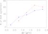 |
Fig. 12. Percentage of stars spectroscopically identified as belonging to the AGB and for which their AGB evolutionary status is in agreement with COR (blue) and ABBA (red) as a function of Δν. Each data point corresponds to the aggregation of the agreement over a Δν range of 0.5 μHz. |
9. Conclusion
The determination of red giant evolutionary status is of primary importance for stellar population, stellar interiors, and galactic archaeology studies. For this paper, we created the most precise and up-to-date red giant evolutionary status catalog for Kepler asteroseismic targets to be used in the future on stellar evolution works and stellar population analysis. We obtained this catalog with asteroseismic and spectroscopic data. We combined several automated asteroseismic evolutionary status determination methods to obtain the final sample separating RC and RGB stars. The different techniques were found to be in very good agreement with each other; those using the mixed-mode pattern were the most accurate but delivered fewer results in general. We compared this determination to the evolutionary status estimation given by spectroscopic results from the APOKASC-3 Kepler sample, which corresponds to a subsample of the red giant Kepler legacy sample. We then focused on this subsample for a more detailed analysis.
We showed that the spectroscopic determination was in very good agreement with the asteroseismic results, therefore proving the robustness of the calibrated spectroscopic evolutionary status determination. The stars for which a disagreement arises between the spectroscopic and asteroseismic classification appeared to have peculiar characteristics for their evolutionary status (high-mass on the RGB, high log(g) for clump targets or stars at the beginning of the AGB branch), therefore explaining why a confusion can arise between the two evolutionary statuses.
This new catalog is in agreement with previous work (Elsworth et al. 2019) and can be used to further test stellar models, including the necessary assumptions on the overshoot amount. We demonstrated that the RC has a clear observable edge situated at 2.99 ± 0.01 in log(g). In agreement with previous results, we identified and confirmed the minimum radius of the zero-age sequence of helium-burning stars (ZAHB), leaving only a few stars with a radius lower than this observed limit. Those stars, as pointed out by Li et al. (2022), likely correspond to peculiar red giants that experienced mass loss during their evolution.
Finally, we tested the possibility of disentangling RGB from AGB stars on the upper part of the giant branch with asteroseismology and spectroscopy. We found that the seismic methods are in agreement with the spectroscopic data on the identification of AGB targets, but only in the vicinity of the RC, for stars with Δν ∼ 2 μHz. The results between the different techniques diverge rapidly when the star evolves along the AGB showing that identifying these stars remains difficult. This work thus shows that the seismically identified AGB targets needs to be used with caution regarding the certainty of their evolutionary status for future works.
Data availability
Full Tables 2 and 4 are available at the CDS via anonymous ftp to cdsarc.cds.unistra.fr (130.79.128.5) or via https://cdsarc.cds.unistra.fr/viz-bin/cat/J/A+A/697/A165
Acknowledgments
M.V. acknowledges support from NASA grant 80NSSC18K1582 and funding from the European Research Council (ERC) under the European Union’s Horizon 2020 research and innovation programme (Grant agreement No. 101019653). R. A. G. acknowledges the support of the PLATO and GOLF grants from the Centre National d’Études Spatiales (CNES). This Paper includes data collected by the Kepler mission and obtained from the MAST data archive at the Space Telescope Science Institute (STScI). Funding for the Kepler mission is provided by the NASA Science Mission Directorate. STScI is operated by the Association of Universities for Research in Astronomy, Inc., under NASA contract NAS 5-26555. M.H. acknowledges support from NASA grant 80NSSC24K0228. D.S. is supported by the Australian Research Council (DP190100666). S.M. acknowledges support by the Spanish Ministry of Science and Innovation with the Ramon y Cajal fellowship number RYC-2015-17697, the grant number PID2019-107187GB-I00, the grants no. PID2019-107061GB-C66 and PID2023-149439NB-C41, and through AEI under the Severo Ochoa Centres of Excellence Programme 2020–2023 (CEX2019-000920-S). S.H. acknowledge funding from the ERC Consolidator Grant DipolarSound (grant agreement # 101000296).
References
- Abdurro’uf, Accetta, K., Aerts, C., et al. 2022, ApJS, 259, 35 [NASA ADS] [CrossRef] [Google Scholar]
- Ahumada, R., Prieto, C. A., Almeida, A., et al. 2020, ApJS, 249, 3 [Google Scholar]
- Arp, H. C., Baum, W. A., & Sandage, A. R. 1953, AJ, 58, 4 [Google Scholar]
- Baglin, A., Auvergne, M., Barge, P., et al. 2006, in The CoRoT Mission Pre-Launch Status - Stellar Seismology and Planet Finding, eds. M. Fridlund, A. Baglin, J. Lochard, & L. Conroy, ESA Special Publication, 1306, 33 [NASA ADS] [Google Scholar]
- Banks, K. A., Ho, C. Y. Y., Martell, S. L., et al. 2023, MNRAS, 523, L80 [Google Scholar]
- Banks, K. A., Martell, S. L., Tinney, C. G., et al. 2024, MNRAS, 529, 3912 [Google Scholar]
- Beck, P. G., Bedding, T. R., Mosser, B., et al. 2011, Science, 332, 205 [Google Scholar]
- Bedding, T. R., Mosser, B., Huber, D., et al. 2011, Nature, 471, 608 [Google Scholar]
- Bonaca, A., Tanner, J. D., Basu, S., et al. 2012, ApJ, 755, L12 [NASA ADS] [CrossRef] [Google Scholar]
- Borucki, W. J., Koch, D., Basri, G., et al. 2010, Science, 327, 977 [Google Scholar]
- Bossini, D., Miglio, A., Salaris, M., et al. 2015, MNRAS, 453, 2290 [Google Scholar]
- Bossini, D., Miglio, A., Salaris, M., et al. 2017, MNRAS, 469, 4718 [Google Scholar]
- Brogaard, K., VandenBerg, D. A., Bruntt, H., et al. 2012, A&A, 543, A106 [NASA ADS] [CrossRef] [EDP Sciences] [Google Scholar]
- Choi, J., Dotter, A., Conroy, C., et al. 2016, ApJ, 823, 102 [Google Scholar]
- Cinquegrana, G. C., Joyce, M., & Karakas, A. I. 2022, ApJ, 939, 50 [Google Scholar]
- Constantino, T., Campbell, S. W., Christensen-Dalsgaard, J., Lattanzio, J. C., & Stello, D. 2015, MNRAS, 452, 123 [Google Scholar]
- Crawford, C. L., Bedding, T. R., Li, Y., et al. 2024, MNRAS, 528, 7397 [NASA ADS] [CrossRef] [Google Scholar]
- Dotter, A. 2016, ApJS, 222, 8 [Google Scholar]
- Dréau, G., Mosser, B., Lebreton, Y., Gehan, C., & Kallinger, T. 2021, A&A, 650, A115 [NASA ADS] [CrossRef] [EDP Sciences] [Google Scholar]
- Dupret, M., Belkacem, K., Samadi, R., et al. 2009, A&A, 506, 57 [NASA ADS] [CrossRef] [EDP Sciences] [Google Scholar]
- Elsworth, Y., Hekker, S., Basu, S., & Davies, G. R. 2017, MNRAS, 466, 3344 [NASA ADS] [CrossRef] [Google Scholar]
- Elsworth, Y., Hekker, S., Johnson, J. A., et al. 2019, MNRAS, 489, 4641 [NASA ADS] [CrossRef] [Google Scholar]
- Gaia Collaboration (Babusiaux, C., et al.) 2018, A&A, 616, A10 [NASA ADS] [CrossRef] [EDP Sciences] [Google Scholar]
- García, R. A., Hekker, S., Stello, D., et al. 2011, MNRAS, 414, L6 [NASA ADS] [CrossRef] [Google Scholar]
- García, R. A., Mathur, S., Pires, S., et al. 2014, A&A, 568, A10 [Google Scholar]
- García Pérez, A. E., Allende Prieto, C., Holtzman, J. A., et al. 2016, AJ, 151, 144 [Google Scholar]
- Girardi, L. 1999, MNRAS, 308, 818 [CrossRef] [Google Scholar]
- Girardi, L. 2016, ARA&A, 54, 95 [Google Scholar]
- Grosjean, M., Dupret, M.-A., Belkacem, K., et al. 2014, A&A, 572, A11 [CrossRef] [EDP Sciences] [Google Scholar]
- Gunn, J. E., Siegmund, W. A., Mannery, E. J., et al. 2006, AJ, 131, 2332 [NASA ADS] [CrossRef] [Google Scholar]
- Handberg, R., Brogaard, K., Miglio, A., et al. 2017, MNRAS, 472, 979 [CrossRef] [Google Scholar]
- Hawkins, K., Ting, Y.-S., & Walter-Rix, H. 2018, ApJ, 853, 20 [NASA ADS] [CrossRef] [Google Scholar]
- Herwig, F. 2000, A&A, 360, 952 [NASA ADS] [Google Scholar]
- Hon, M., Stello, D., & Yu, J. 2017, MNRAS, 469, 4578 [NASA ADS] [CrossRef] [Google Scholar]
- Hon, M., Stello, D., & Yu, J. 2018, MNRAS, 476, 3233 [NASA ADS] [CrossRef] [Google Scholar]
- Howell, M., Campbell, S. W., Stello, D., & De Silva, G. M. 2022, MNRAS, 515, 3184 [NASA ADS] [CrossRef] [Google Scholar]
- Howell, M., Campbell, S. W., Stello, D., & De Silva, G. M. 2024, MNRAS, 527, 7974 [Google Scholar]
- Howell, M., Campbell, S. W., Kalup, C., Stello, D., & De Silva, G. M. 2025, MNRAS, 536, 1389 [Google Scholar]
- Jönsson, H., Holtzman, J. A., Allende Prieto, C., et al. 2020, AJ, 160, 120 [Google Scholar]
- Joyce, M., & Chaboyer, B. 2018, ApJ, 856, 10 [Google Scholar]
- Joyce, M., & Tayar, J. 2023, Galaxies, 11, 75 [NASA ADS] [CrossRef] [Google Scholar]
- Kallinger, T. 2019, ArXiv e-prints [arXiv:1906.09428] [Google Scholar]
- Kallinger, T., Weiss, W. W., Barban, C., et al. 2010, A&A, 509, A77 [CrossRef] [EDP Sciences] [Google Scholar]
- Kallinger, T., Hekker, S., Mosser, B., et al. 2012, A&A, 541, A51 [NASA ADS] [CrossRef] [EDP Sciences] [Google Scholar]
- Karakas, A. I., Cinquegrana, G., & Joyce, M. 2022, MNRAS, 509, 4430 [Google Scholar]
- Kjeldsen, H., & Bedding, T. R. 1995, A&A, 293, 87 [NASA ADS] [Google Scholar]
- Kuszlewicz, J. S., Hekker, S., & Bell, K. J. 2020, MNRAS, 497, 4843 [NASA ADS] [CrossRef] [Google Scholar]
- Lagarde, N., Bossini, D., Miglio, A., Vrard, M., & Mosser, B. 2016, MNRAS, 457, L59 [NASA ADS] [CrossRef] [Google Scholar]
- Li, Y., Bedding, T. R., Stello, D., et al. 2021, MNRAS, 501, 3162 [NASA ADS] [CrossRef] [Google Scholar]
- Li, Y., Bedding, T. R., Murphy, S. J., et al. 2022, Nature Astronomy, 6, 673 [Google Scholar]
- Majewski, S. R., Schiavon, R. P., Frinchaboy, P. M., et al. 2017, AJ, 154, 94 [NASA ADS] [CrossRef] [Google Scholar]
- Miglio, A., Brogaard, K., Stello, D., et al. 2012, MNRAS, 419, 2077 [Google Scholar]
- Miglio, A., Chiappini, C., Mackereth, J. T., et al. 2021, A&A, 645, A85 [NASA ADS] [CrossRef] [EDP Sciences] [Google Scholar]
- Montalbán, J., Miglio, A., Noels, A., et al. 2013, ApJ, 766, 118 [Google Scholar]
- Mosser, B., & Appourchaux, T. 2009, A&A, 508, 877 [NASA ADS] [CrossRef] [EDP Sciences] [Google Scholar]
- Mosser, B., Barban, C., Montalbán, J., et al. 2011a, A&A, 532, A86 [NASA ADS] [CrossRef] [EDP Sciences] [Google Scholar]
- Mosser, B., Belkacem, K., Goupil, M., et al. 2011b, A&A, 525, L9 [CrossRef] [EDP Sciences] [Google Scholar]
- Mosser, B., Elsworth, Y., Hekker, S., et al. 2012a, A&A, 537, A30 [NASA ADS] [CrossRef] [EDP Sciences] [Google Scholar]
- Mosser, B., Goupil, M. J., Belkacem, K., et al. 2012b, A&A, 540, A143 [NASA ADS] [CrossRef] [EDP Sciences] [Google Scholar]
- Mosser, B., Dziembowski, W. A., Belkacem, K., et al. 2013, A&A, 559, A137 [CrossRef] [EDP Sciences] [Google Scholar]
- Mosser, B., Benomar, O., Belkacem, K., et al. 2014, A&A, 572, L5 [NASA ADS] [CrossRef] [EDP Sciences] [Google Scholar]
- Mosser, B., Vrard, M., Belkacem, K., Deheuvels, S., & Goupil, M. J. 2015, A&A, 584, A50 [NASA ADS] [CrossRef] [EDP Sciences] [Google Scholar]
- Mosser, B., Belkacem, K., Pinçon, C., et al. 2017, A&A, 598, A62 [NASA ADS] [CrossRef] [EDP Sciences] [Google Scholar]
- Mosser, B., Michel, E., Samadi, R., et al. 2019, A&A, 622, A76 [NASA ADS] [CrossRef] [EDP Sciences] [Google Scholar]
- Ness, M., Hogg, D. W., Rix, H. W., Ho, A. Y. Q., & Zasowski, G. 2015, ApJ, 808, 16 [NASA ADS] [CrossRef] [Google Scholar]
- Paxton, B., Bildsten, L., Dotter, A., et al. 2011, ApJS, 192, 3 [Google Scholar]
- Paxton, B., Cantiello, M., Arras, P., et al. 2013, ApJS, 208, 4 [Google Scholar]
- Paxton, B., Marchant, P., Schwab, J., et al. 2015, ApJS, 220, 15 [Google Scholar]
- Paxton, B., Schwab, J., Bauer, E. B., et al. 2018, ApJS, 234, 34 [NASA ADS] [CrossRef] [Google Scholar]
- Pinsonneault, M. H., Kawaler, S. D., Sofia, S., & Demarque, P. 1989, ApJ, 338, 424 [Google Scholar]
- Pinsonneault, M. H., An, D., Molenda-Żakowicz, J., et al. 2012, ApJS, 199, 30 [Google Scholar]
- Pinsonneault, M. H., Elsworth, Y., Epstein, C., et al. 2014, ApJS, 215, 19 [Google Scholar]
- Pinsonneault, M. H., Elsworth, Y. P., Tayar, J., et al. 2018, ApJS, 239, 32 [Google Scholar]
- Pinsonneault, M. H., Zinn, J. C., Tayar, J., et al. 2025, ApJS, 276, 69 [NASA ADS] [CrossRef] [Google Scholar]
- Roberts, J. D., Pinsonneault, M. H., Johnson, J. A., et al. 2024, MNRAS, 530, 149 [Google Scholar]
- Salaris, M., Cassisi, S., Schiavon, R. P., & Pietrinferni, A. 2018, A&A, 612, A68 [NASA ADS] [CrossRef] [EDP Sciences] [Google Scholar]
- Shetrone, M., Bizyaev, D., Lawler, J. E., et al. 2015, ApJS, 221, 24 [Google Scholar]
- Smith, V. V., Bizyaev, D., Cunha, K., et al. 2021, AJ, 161, 254 [NASA ADS] [CrossRef] [Google Scholar]
- Stancliffe, R. J., Izzard, R. G., & Tout, C. A. 2005, MNRAS, 356, L1 [Google Scholar]
- Stello, D., Huber, D., Bedding, T. R., et al. 2013, ApJ, 765, L41 [CrossRef] [Google Scholar]
- Stello, D., Compton, D. L., Bedding, T. R., et al. 2014, ApJ, 788, L10 [NASA ADS] [CrossRef] [Google Scholar]
- Stello, D., Cantiello, M., Fuller, J., Garcia, R. A., & Huber, D. 2016, PASA, 33, e011 [Google Scholar]
- Tayar, J., & Pinsonneault, M. H. 2018, ApJ, 868, 150 [Google Scholar]
- Tayar, J., Somers, G., Pinsonneault, M. H., et al. 2017, ApJ, 840, 17 [NASA ADS] [CrossRef] [Google Scholar]
- Tayar, J., Claytor, Z. R., Huber, D., & van Saders, J. 2022, ApJ, 927, 31 [NASA ADS] [CrossRef] [Google Scholar]
- van Saders, J. L., & Pinsonneault, M. H. 2012, ApJ, 746, 16 [NASA ADS] [CrossRef] [Google Scholar]
- Vrard, M., Mosser, B., Barban, C., et al. 2015, A&A, 579, A84 [CrossRef] [EDP Sciences] [Google Scholar]
- Vrard, M., Mosser, B., & Samadi, R. 2016, A&A, 588, A87 [CrossRef] [EDP Sciences] [Google Scholar]
- Vrard, M., Kallinger, T., Mosser, B., et al. 2018, A&A, 616, A94 [NASA ADS] [CrossRef] [EDP Sciences] [Google Scholar]
- Warfield, J. T., Zinn, J. C., Schonhut-Stasik, J., et al. 2024, AJ, 167, 208 [NASA ADS] [CrossRef] [Google Scholar]
- Wilson, J. C., Hearty, F. R., Skrutskie, M. F., et al. 2019, PASP, 131, 055001 [NASA ADS] [CrossRef] [Google Scholar]
- Zasowski, G., Cohen, R. E., Chojnowski, S. D., et al. 2017, AJ, 154, 198 [Google Scholar]
All Tables
Number of evolutionary status results given by the different seismic methods for the red giant Kepler legacy sample (Garcia et al., in preparation) and the APOKASC-3 (Pinsonneault et al. 2025) stars.
Stars for which a conflict is present between the different evolutionary status that was given by the different seismic methods.
First lines of a joined file summarizing the AGB or RGB evolutionary status determination.
All Figures
|
Fig. 1. Stellar surface gravity as a function of the effective temperature Teff for the stars classified as having a robust evolutionary status. The red stars represent the RC and the blue stars represent the RGB or AGB stars for high-luminosity targets. |
| In the text | |
|
Fig. 2. Spectroscopic stellar surface gravity as a function of the effective temperature Teff for the stars having an undetermined evolutionary status (5276 APOKASC-3 targets) and a duration of observation higher than 4 months (3670 APOKASC-3 targets, in black). The green dots correspond to the stars that have a length of observation equal to or lower than 3 months. |
| In the text | |
|
Fig. 3. Distribution of stars as a function of Tref. The blue and red histograms correspond respectively to RGB/AGB and RC stars, as determined by seismology following Section 4. |
| In the text | |
|
Fig. 4. Stellar surface gravity as a function of the effective temperature Teff for the stars showing agreement between the spectroscopic and seismic evolutionary status classification. The red stars represent the RC and the blue stars represent the RGB or AGB stars for high-luminosity objects. |
| In the text | |
|
Fig. 5. Stellar surface gravity as a function of the effective temperature Teff for the stars with an agreement between the spectroscopic and seismic evolutionary status classification (in black). Top: Stars with divergent spectroscopic and seismic evolutionary status (pink triangles). Center: Stars identified as RGB by seismology and RC by spectroscopy for which the evolutionary status was confirmed as RGB (blue triangles) or RC (red triangles). Bottom: Same as center panel, but the red triangles correspond to confirmed RC stars identified as RC by seismology and RGB by spectroscopy. |
| In the text | |
|
Fig. 6. Top: Seismic surface gravity (g) for the stars identified by seismology as belonging to the RC (in red) as a function of the spectroscopic surface gravity. The blue points correspond to the stars identified as RGB by spectroscopy on the contrary to seismic results. Bottom: Seismic surface gravity for the same sample of seismic RC stars, focused on the bottom of the RC. The dashed lines correspond to the maximum values for secondary clump YREC models, with a core overshoot of 0.2 pressure scale height: dark red, cyan, dark green, and pink correspond respectively to stellar models with masses of 3.0, 2.8, 2.6, and 2.4 M⊙. |
| In the text | |
|
Fig. 7. Seismic radius as a function of seismic mass for stars identified as RC following Section 4. The maximum log(g) values of the RC for the different YREC models are represented by the diamonds. The colors depict models with different core overshooting values: no overshooting (dark green), 0.1 pressure scale height (cyan), and 0.2 pressure scale height (dark blue). The minimum radius values for the different MIST tracks are shown as black crosses. |
| In the text | |
|
Fig. 8. Difference between the star Teff and the reference model effective temperature Tint as a function of metallicity. The Teff and metallicity values are from the APOKASC-3 sample. |
| In the text | |
|
Fig. 9. Distribution of stars identified as RGB or AGB, with log(g) < 2.2 (stars above the main RC population in a Kiel diagram) as a function of ΔTref (in blue). The dot-dashed red line shows a Gaussian fit of width 44.04 K centered on −26.40 following the distribution of α-rich stars. The orange dashed line indicates the two-σ limit of the measured RGB sample distribution following Section 5. |
| In the text | |
|
Fig. 10. log(g) as a function of ΔTref for the stars above the main RC population. The blue points correspond to the stars identified as RGB targets, the orange points represent stars where the evolutionary status is uncertain, and the red points are AGB candidates. The overplotted solid red and blue lines show the AGB-RGB Teff offset for, respectively, the 1.7 M⊙ and 1.0 M⊙ MIST evolutionary track. Top: full APOKASC-3 sample. Middle: α-poor targets. Bottom: α-rich targets. |
| In the text | |
|
Fig. 11. log(g) as a function of Teff for the stars above the main RC population. The blue points correspond to the stars identified as RGB targets, the orange points represent stars where the evolutionary status is uncertain, and the red points are AGB candidates. Top: full APOKASC-3 sample. Middle: α-poor targets. Bottom: α-rich targets. |
| In the text | |
|
Fig. 12. Percentage of stars spectroscopically identified as belonging to the AGB and for which their AGB evolutionary status is in agreement with COR (blue) and ABBA (red) as a function of Δν. Each data point corresponds to the aggregation of the agreement over a Δν range of 0.5 μHz. |
| In the text | |
Current usage metrics show cumulative count of Article Views (full-text article views including HTML views, PDF and ePub downloads, according to the available data) and Abstracts Views on Vision4Press platform.
Data correspond to usage on the plateform after 2015. The current usage metrics is available 48-96 hours after online publication and is updated daily on week days.
Initial download of the metrics may take a while.