| Issue |
A&A
Volume 616, August 2018
|
|
|---|---|---|
| Article Number | A24 | |
| Number of page(s) | 12 | |
| Section | Stellar structure and evolution | |
| DOI | https://doi.org/10.1051/0004-6361/201832822 | |
| Published online | 07 August 2018 | |
Core rotation braking on the red giant branch for various mass ranges
1
PSL, LESIA, CNRS, Université Pierre et Marie Curie, Université Denis Diderot, Observatoire de Paris,
92195
Meudon Cedex,
France
e-mail: This email address is being protected from spambots. You need JavaScript enabled to view it.
2
Institute for Astrophysics, University of Vienna,
Türkenschanzstrasse 17,
1180
Vienna,
Austria
Received:
13
February
2018
Accepted:
8
April
2018
Abstract
Context. Asteroseismology allows us to probe stellar interiors. In the case of red giant stars, conditions in the stellar interior are such as to allow for the existence of mixed modes, consisting in a coupling between gravity waves in the radiative interior and pressure waves in the convective envelope. Mixed modes can thus be used to probe the physical conditions in red giant cores. However, we still need to identify the physical mechanisms that transport angular momentum inside red giants, leading to the slow-down observed for red giant core rotation. Thus large-scale measurements of red giant core rotation are of prime importance to obtain tighter constraints on the efficiency of the internal angular momentum transport, and to study how this efficiency changes with stellar parameters.
Aims. This work aims at identifying the components of the rotational multiplets for dipole mixed modes in a large number of red giant oscillation spectra observed by Kepler. Such identification provides us with a direct measurement of the red giant mean core rotation.
Methods. We compute stretched spectra that mimic the regular pattern of pure dipole gravity modes. Mixed modes with the same azimuthal order are expected to be almost equally spaced in stretched period, with a spacing equal to the pure dipole gravity mode period spacing. The departure from this regular pattern allows us to disentangle the various rotational components and therefore to determine the mean core rotation rates of red giants.
Results. We automatically identify the rotational multiplet components of 1183 stars on the red giant branch with a success rate of 69% with respect to our initial sample. As no information on the internal rotation can be deduced for stars seen pole-on, we obtain mean core rotation measurements for 875 red giant branch stars. This large sample includes stars with a mass as large as 2.5 M⊙, allowing us to test the dependence of the core slow-down rate on the stellar mass.
Conclusions. Disentangling rotational splittings from mixed modes is now possible in an automated way for stars on the red giant branch, even for the most complicated cases, where the rotational splittings exceed half the mixed-mode spacing. This work on a large sample allows us to refine previous measurements of the evolution of the mean core rotation on the red giant branch. Rather than a slight slow-down, our results suggest rotation is constant along the red giant branch, with values independent of the mass.
Key words: asteroseismology / methods: data analysis / stars: interiors / stars: oscillations / stars: rotation / stars: solar-type
© ESO 2018
 Open Access article, published by EDP Sciences, under the terms of the Creative Commons Attribution License (http://creativecommons.org/licenses/by/4.0;), which permits unrestricted use, distribution, and reproduction in any medium, provided the original work is properly cited.
1 Introduction
The ultra-high precision photometric space missions CoRoT and Kepler have recorded extremely long observation runs, providing us with seismic data of unprecedented quality. The surprise came from red giant stars (e.g. Mosser & Miglio 2016), which present solar-like oscillations that are stochastically excited in the external convective envelope (Dupret et al. 2009). Oscillation power spectra showed that red giants not only present pressure modes as in the Sun, but also mixed modes (De Ridder et al. 2009; Bedding et al. 2011) resulting from a coupling of pressure waves in the outer envelope with internal gravity waves (Scuflaire 1974). As mixed modes behave as pressure modes in the convective envelope and as gravity modes in the radiative interior, they allow one to probe the core of red giants (Beck et al. 2011).
Dipole mixed modes are particularly interesting because they are mostly sensitive to the red giant core (Goupil et al. 2013). They were used to automatically measure the dipole gravity mode period spacing ΔΠ1 for almost 5000 red giants (Vrard et al. 2016), providing information about the size of the radiative core (Montalbán et al. 2013) and defined as
 (1)
(1)
where NBV is the Brunt–Väisälä frequency. The measurement of ΔΠ1 leads to the accurate determination of the stellar evolutionary stage and allows us to distinguish shell-hydrogen-burning red giants from core-helium-burning red giants (Bedding et al. 2011; Stello et al. 2013; Mosser et al. 2014).
Dipole mixed modes also give access to near-core rotation rates (Beck et al. 2011). Rotation has been shown to impact not only the stellar structure by perturbing the hydrostatic equilibrium, but also the internal dynamics of stars by means of the transport of both angular momentum and chemical species (Zahn 1992; Talon & Zahn 1997; Lagarde et al. 2012). It is thus crucial to measure this parameter for a large number of stars to monitor its effect on stellar evolution (Lagarde et al. 2016). Semi-automatic measurements of the mean core rotation of about 300 red giants indicated that their cores are slowing down along the red giant branch while contracting at the same time (Mosser et al. 2012b; Deheuvels et al. 2014). Thus, angular momentum is efficiently extracted from red giant cores (Eggenberger et al. 2012; Cantiello et al. 2014), but the physical mechanisms supporting this angular momentum transport are not yet fully understood. Indeed, several physical mechanisms transportingangular momentum have been implemented in stellar evolutionary codes, such as meridional circulation and shear turbulence (Eggenberger et al. 2012; Marques et al. 2013; Ceillier et al. 2013), mixed modes (Belkacem et al. 2015a,b), internal gravity waves (Fuller et al. 2014; Pinçon et al. 2017), and magnetic fields (Cantiello et al. 2014; Rüdiger et al. 2015), but none of them can reproduce the measured orders of magnitude for the core rotation along the red giant branch. In parallel, several studies have tried to parameterize the efficiency of the angular momentum transport inside red giants through ad-hoc diffusion coefficients (Spada et al. 2016; Eggenberger et al. 2017).
In this context, we need to obtain mean core rotation measurements for a much larger set of red giants in order to put stronger constraints on the efficiency of the angular momentum transport and to study how this efficiency changes with the global stellar parameters like mass (Eggenberger et al. 2017). In particular, we require measurements for stars on the red giant branch because the dataset analysed by Mosser et al. (2012b) only includes 85 red giant branch stars. The absence of large-scale measurements is due to the fact that rotational splittings often exceed half the mixed-mode frequency spacings at low frequencies in red giants. For such conditions, disentangling rotational splittings from mixed modes is challenging. Nevertheless, it is of prime importance to develop a method as automated as possible as we enter the era of massive photometric data, with Kepler providing light curves for more than 15 000 red giant stars and the future Plato mission potentially increasing this number to hundreds of thousands.
In this work we set up an almost fully automated method to identify the rotational signature of stars on the red giant branch. Our method is not suitable for clump stars, presenting smaller rotational splittings as well as larger mode widths due to shorter lifetimes of gravity modes (Vrard et al. 2017). Thus, the analysis of the core rotation of clump stars is beyond the scope of this paper. In Sect. 2 we explain the principle of the method, based on the stretching of frequency spectra to obtain period spectra reproducing the evenly-spaced gravity-mode pattern. In Sect. 3 we detail the set up of the method, including the estimation of the uncertainties. In Sect. 4 we compare our results with those obtained by Mosser et al. (2012b). In Sect. 5 we apply the method to red giant branch stars of the Kepler public catalogue, and investigate the impact of the stellar mass on the evolution of the core rotation. Section 6 is devoted to discussion and Sect. 7 to conclusions.
2 Principle of the method
Mixed modes have a dual nature: pressure-dominated mixed modes (p-m modes) are almost equally spaced in frequency, with a frequency spacing close to the large separation Δν, while gravity-dominated mixed modes (g-m modes) are almost equally spaced in period, with a period spacing close to Δ Π1. In order to retrieve the behaviour of pure gravity modes, we need to disentangle the different contributions of p-m and g-m modes, which can be done by deforming the frequency spectra.
2.1 Stretching frequency spectra
The mode frequencies of pure pressure modes are estimated through the red giant universal oscillation pattern (Mosser et al. 2011)
 (2)
(2)
where
np is the pressure radial order;
ℓ is the angular degree of the oscillation mode;
εp is the phase shift of pure pressure modes;
α represents the curvature of the radial oscillation pattern;
d0ℓ is the small separation, namely the distance, in units of Δν, of the pure pressure mode having an angular degree equal to ℓ, compared to the midpoint between the surrounding radial modes;
nmax = νmax∕Δν − εp is the non-integer order at the frequency νmax of maximum oscillation signal.
We consider only dipole mixed modes, which are mainly sensitive to the red giant core. Thus, in a first step we remove from the observed spectra the frequency ranges where radial and quadrupole modes are expected using the universal oscillation pattern (Eq. (2)). We then convert the frequency spectra containing only dipole mixed modes into stretched period spectra, with the stretched period τ derived from the differential equation (Mosser et al. 2015):
 (3)
(3)
The ζ function, introduced by Goupil et al. (2013) as a function of mode inertia, expressed as a function of global asymptotic parameters by Mosser et al. (2015), can be redefined as (Hekker & Christensen-Dalsgaard 2017)
![Mathematical equation: \begin{equation*}\zeta = \left[1 + \frac{\nu^2}{q} \frac{{\mathrm \Delta}{\mathrm \Pi}_{{1}}}{{\mathrm \Delta}\nu_{\textrm{p}}} \frac{1}{\frac{1}{q^2} \sin^2 \left(\pi \frac{\nu - \nu_{\textrm{p}}}{{\mathrm \Delta}\nu_{\textrm{p}}}\right) + \cos^2 \left(\pi \frac{\nu - \nu_{\textrm{p}}}{{\mathrm \Delta}\nu_{\textrm{p}}}\right)}\right]^{-1}. \end{equation*}](/articles/aa/full_html/2018/08/aa32822-18/aa32822-18-eq4.png) (4)
(4)
The parameters entering the definition of ζ are as follows:
q the coupling parameter between gravity and pressure modes;
 the observed large separation, which increases with the radial order;
νp the puredipole pressure mode frequencies;
ν the mixed-mode frequencies.
The pure dipole pressure mode frequencies are given by Eq. (2) for ℓ = 1. The mixed-modefrequencies are given by the asymptotic expansion of mixed modes (Mosser et al. 2012c):
![Mathematical equation: \begin{equation*}\nu = \nu_{\textrm{p}} + \frac{{\mathrm \Delta}\nu_{\textrm{p}}}{\pi} \arctan \left[q \tan \pi \left( \frac{1}{{\mathrm \Delta}{\mathrm \Pi}_{{1}} \nu} - \frac{1}{{\mathrm \Delta}{\mathrm \Pi}_{{1}} \nu_{\textrm{g}}} \right) \right], \end{equation*}](/articles/aa/full_html/2018/08/aa32822-18/aa32822-18-eq6.png) (5)
(5)
where
 (6)
(6)
are the pure dipole gravity mode frequencies, with ng being the gravity radial order, usually defined as a negative integer.
We can approximate
 (7)
(7)
where ΔP is the bumped period spacing between consecutive dipole mixed modes. In these conditions, ζ gives information on the trapping of dipole mixed modes. Gravity-dominated mixed modes (g-m modes) have a period spacing close to Δ Π1 and represent the local maxima of ζ, while pressure-dominated mixed modes (p-m modes) have a lower period spacing decreasing with frequency and represent the local minima of ζ (Fig. 1).
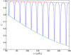 |
Fig. 1 Stretching function ζ (blue line) computed with Δν = 11 μHz, Δ Π1 = 80 s, and q = 0.12. The asymptotic behaviours of ζ for g-m and p-m modes are indicated by a red and green line, respectively. |
2.2 Revealing the rotational components
Pressure-dominated mixed modes are not only sensitive to the core but also to the envelope. The next step thus consists in removing p-m modes from the spectra through Eq. (2), leaving only g-m modes. In practice, g-m modes with a height-to-background ratio larger than six are considered as significant in a first step; then this threshold is manually adapted in order to obtain the best compromise between the number of significant modes and background residuals. All dipole g-m modes with the same azimuthal order m should thenbe equally spaced in stretched period, with a spacing close to Δ Π1. However, the core rotation perturbs this regular pattern so that the stretched period spacing between consecutive g-m modes with the same azimuthal order slightly differs from ΔΠ1, with the small departure depending on the mean core rotational splitting as (Mosser et al. 2015)
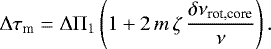 (8)
(8)
As the meanvalue of ζ depends on the mixed-mode density  , we can avoid the calculation of ζ by approximating
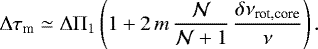 (9)
(9)
The mixed-mode density represents the number of gravity modes per Δ ν-wide frequency range and is defined as
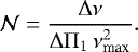 (10)
(10)
Red giants are slow rotators, presenting low rotation frequencies of the order of 2 μHz or less. In these conditions, the centrifugal acceleration can be neglected everywhere in red giants (Goupil et al. 2013). Besides, Ω (r)∕2π < Δν ≪ νmax throughout the whole star and Coriolis effects are negligible. Thus, rotation can be treated as a first-order perturbation of the hydrostatic equilibrium (Ouazzani et al. 2013), and the rotational splitting can be written as follows (Unno et al. 1989; see also Goupil et al. 2013 for the case of red giants):
 (11)
(11)
where x = r∕R is the normalized radius, K(x) is the rotational kernel, and Ω(x) is the angular velocity at normalized radius x. In a first approximation, we can separate the core and envelope contributions of the rotational splitting as
 (12)
(12)
with
![Mathematical equation: \begin{eqnarray}&&\hskip-4pt\beta_{\textrm{core}} = \int_{0}^{x _{\textrm{core}}} K(x) \textrm{d} x,\\[1pt] &&\hskip-4pt\beta_{\textrm{env}} = \int_{x _{\textrm{core}}}^{1} K(x) \textrm{d} x,\\[1pt] &&\hskip-4pt\langle{\mathrm \Omega}\rangle_{\textrm{core}} = \frac{\int_{0}^{x_{\textrm{core}}} {\mathrm \Omega}(x) K(x) \textrm{d} x}{\int_{0}^{x_{\textrm{core}}} K(x) \textrm{d} x},\\[1pt] &&\hskip-4pt\langle{\mathrm \Omega}\rangle_{\textrm{env}} = \frac{\int_{x_{\textrm{core}}}^{1} {\mathrm \Omega}(x) K(x) \textrm{d} x}{\int_{x_{\textrm{core}}}^{1} K(x) \textrm{d} x},\end{eqnarray}](/articles/aa/full_html/2018/08/aa32822-18/aa32822-18-eq15.png)
xcore = rcore∕R being the normalized radius of the g-mode cavity.
If we assume that dipole g-m modes are mainly sensitive to the core, we can neglect the envelope contribution as βcore∕βenv ≫ 1 in these conditions. Moreover, βcore ≃ 1∕2 for dipole g-m modes (Ledoux 1951). In these conditions, a linear relation connects the core rotational splitting to the mean core angular velocity as follows (Goupil et al. 2013; Mosser et al. 2015)
 (17)
(17)
The departure of Δτm from Δ Π1 is small, on the order of a few percent of Δ Π1. This allows us to fold the stretched spectrum with ΔΠ1 in order to build stretched period échelle diagrams (Mosser et al. 2015), in which the individual rotational components align according to their azimuthal order and become easy to identify (Fig. 2). When the star is seen pole-on, the m = 0 components line up on a unique and almost vertical ridge. Rotation modifies this scheme by splitting mixed modes into two or three components, depending on the stellar inclination.
In theseéchelle diagrams, rotational splittings and mixed modes are now disentangled. It is possible to identify the azimuthal order of each component of a rotational multiplet, even in a complex case like KIC 10866415 where the rotational splitting is much larger than the mixed-mode frequency spacing. In such cases, the ridges cross each other (Fig. 2).
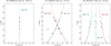 |
Fig. 2 Stretched period échelle diagrams for red giant branch stars with different inclinations. The rotational components are identified in an automatic way through a correlation of the observed spectrum with a synthetic one constructed using Eq. (9). The colours indicate the azimuthal order: the m = {−1, 0, +1} rotationalcomponents are represented in green, light blue, and red, respectively. The symbol size varies as the power spectral density. Left panel: star seen pole-on where only the m = 0 rotational component is visible. Middle panel: star seen equator-on where the m = {−1, +1} componentsare visible. Right panel: star with an intermediate inclination angle where all the three components are visible. |
3 Disentangling and measuring rotational splittings
We use stretched period échelle diagrams to develop an automated identification of rotational multiplet components. The method is based on a correlation between the observed spectrum and a synthetic one.
3.1 Construction of synthetic spectra
Synthetic spectra are built from Eqs. (9) and (10). Frequencies corresponding to pure gravity modes unperturbed by rotation, associated with the azimuthal order m = 0, are first constructed through Eq. (6). Rotation perturbs and shifts oscillation frequencies of g-m modes associated with azimuthal orders m such as ν − m ζδνrot,core (Mosser et al. 2015). Once frequencies have been built for g-m modes associated with m = {−1, 0, +1}, periods are calculated through P = 1∕ν and are used to construct synthetic stretched periods through Eqs. (9) and (10).
Figure 3 shows examples of such synthetic échelle diagrams for two different δνrot,core values, where the rotational components present many crossings. These crossings between multiplet rotational components with different azimuthal orders are similar to what was shown by Ouazzani et al. (2013) for theoretical red giant spectra. However, they occur here at a smaller core pulsation frequency, for 200 < ⟨Ωcore⟩∕2π < 2000 nHz, while Ouazzani et al. (2013) found the first crossings to happen around ⟨Ωcore⟩∕2π = 8 μHz.
The frequencies where crossings occur can be expressed as (Gehan et al. 2017)
 (18)
(18)
where k is a positive integer representing the crossing order. We can define whether a red giant is a slow or a rapid rotator by comparing δνrot,core to half the mixed-mode frequency spacing, which can be approximated by  (Gehan et al. 2017). In these conditions, the échelle diagram shown in Fig. 3 for the largest rotational splitting can be understood as follows. The upper part corresponds to slow rotators with no crossing, where
  . These cases can be found on the lower giant branch. The medium part, where the first crossing occurs, corresponds to moderate rotators where
  . Such complicated cases are found at lower frequencies, corresponding to most of the evolved stars in the Kepler sample, where rotational components can now be clearly disentangled through the use of the stretched period. The lower part corresponds to rapid rotators, where
  and too many crossings occur to allow the identification of the multiplet components in the unperturbed frequency spectra. Nevertheless, rotational components can still be disentangled using stretched period spectra. The lowest part corresponds to very rapid rotators with too many crossings to allow the identification of the multiplet rotational components, for which currently no measurement of the core rotation is possible.
For fixed νmax and ΔΠ1 values, the more δνrot,core increases, the more δνrot,core becomes larger compared to  . Thus, the pattern presented in Fig. 3 is shifted upwards towards higher frequencies. In practice, if we consider stars that have the same ΔΠ1 and νmax, the larger the rotational splitting, the higher the crossing frequencies, and the larger the number of visible crossings.
Such synthetic échelle diagrams were originally used to identify the crossing order for stars with overlapping multiplet rotational components (Gehan et al. 2017). Combined with the measurement of at least one frequency where a crossing occurs, the identification of the crossing order provides us with a measurement of the mean core rotational splitting. In this study, we base our work on this method, extending it to allow for the identification of the rotational multiplet components whether these components overlap or not.
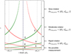 |
Fig. 3 Synthetic stretched period échelle diagram built from Eqs. (9) and (10). The colours indicate the azimuthal order: the m = {−1, 0, +1} rotational components are given by green triangles, blue dots, and red crosses, respectively. The small black dots represent
|
3.2 Correlation of the observed spectrum with synthetic ones
The observed spectrum is correlated with different synthetic spectra constructed with different δνrot,core and Δ Π1 values, through an iterative process. The position of the synthetic spectra is based on the position of important peaks in the observed spectra, defined as having a power spectral density greater than or equal to 0.25 times the maximal power spectral density of g-m modes.
We test δνrot,core values ranging from 100 nHz to 1 μHz with steps of 5 nHz. In fact, the method is not adequate for δνrot,core < 100 nHz and for δνrot,core > 1 μHz: when δνrot,core is too low, the multiplet rotational components are too close to be unambiguously distinguished in échelle diagrams; when δνrot,core is too high, the multiplet rotational components overlap over several g-m mode orders, making their identification challenging.
We also considered ΔΠ1 as a flexible parameter. We used the ΔΠ1 measurements of Vrard et al. (2016) as a first guess and tested Δ Π1,test in the range Δ Π1 (1 ± 0.03) with steps of 0.1 s. Indeed, inaccurate ΔΠ1 measurements can occur when only a low number of g-m modes are observed, due to suppressed dipole modes (Mosser et al. 2017) or high up the giant branch where g-m modes have a very high inertia and cannot be observed (Grosjean et al. 2014). Moreover, even small variations of the folding period Δ Π1 modify the inclination of the observed ridges in the échelle diagram. They are then no longer symmetric with respect to the vertical m = 0 ridge if the folding period ΔΠ1 is not precise enough, and the correlation with synthetic spectra may fail. Thus, our correlation method not only gives high-precision δνrot,core measurements, but also allows us to improve the precision on the measurement of Δ Π1, expected to be as good as 0.01%.
Furthermore, the stellar inclination is not known a priori and impacts the number of visible rotationally split frequency components in the spectum. Thus, three types of synthetic spectra are tested at each time step, containing one, two, and three rotational multiplet components.
3.3 Selection of the best-fitting synthetic spectrum
For each configuration tested, namely for synthetic spectra including one, two, or three components, the best fit is selected in an automated way by maximizing the number of peaks aligned with the synthetic ridges. After this automated step, an individual check is performed to select the best solution, depending on the number of rotational components. This manual operation allows us to correct for the spurious signatures introduced by short-lived modes or ℓ = 3 modes.
We define τpeak and τsynt as the observed and synthetic stretched periods of any given peak, respectively. We empirically consider that a peak is aligned with a synthetic ridge if
 (19)
(19)
We further define
 (20)
(20)
where n is the total number of aligned peaks along the synthetic ridges and χ2 is the mean residual squared sum for peaks belonging to the synthetic rotational multiplet components. The χ2 quantity thus represents an estimate of the spread of the observed τpeak values around the synthetic τsynth. If several δνrot,core and ΔΠ1,test values give the same number of aligned peaks, then the best fit corresponds to the minimum χ2 value.
This step provides us with the best values of ΔΠ1,test and δνrot,core for each of the three stellar inclinations tested. At this stage, at most three possible synthetic spectra remain, corresponding to fixed Δ Π1,test and δνrot,core values: a spectrum with one, two, or three rotational multiplet components. The final fit corresponding to the actual configuration is selected manually. Such final fits shown in Fig. 2 provide us with a measurement of the mean core rotational splitting, except when the star is nearby pole-on.
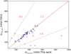 |
Fig. 4 Comparison of the present results with those from Mosser et al. (2012b) for stars on the red giant branch. The solid red line represents the 1:1 relation. The red dashed lines represent the 1:2 and 2:1 relations. |
3.4 Uncertainties
The uncertainty σ on the measurement of δνrot,core is calculatedthrough Eq. (20), except that peaks with
 (21)
(21)
are considered as non-significant and are discarded from the estimation of the uncertainties. They might be due to background residuals, to ℓ = 1 p-m modes that were not fully discarded, or to ℓ = 3 modes. The obtained uncertainties are on the order of 10 nHz or smaller.
4 Comparison with other measurements
Mosser et al. (2012b) measured the mean core rotation of about 300 stars, both on the red giant branch (RGB) and in the red clump. We apply our method to the RGB stars of Mosser et al. (2012b) sample, representing 85 stars. The method proposed a satisfactory identification of the rotational components in 79% of cases. Nevertheless, for some cases our method detects only the m = 0 component while Mosser et al. (2012b) obtained a measurement of the mean core rotation, which requires the presence of m = ± 1 components in the observations. Finally, our method provides δνrot,core measurements for 67% of the stars in the sample. Taking as a reference the measurements of Mosser et al. (2012b), we can thus estimate that we miss about 12% of the possible δνrot,core measurements by detecting only the m = 0 rotational component, while the m = ± 1 components are also present but remain undetected by our method. This mostly happens at low inclination values, when the visibility of the m = ± 1 components is very low compared to that of m = 0. In such cases, the components associated with m = ± 1 appear to us lost in the background noise.
We calculated the relative difference between the present measurements and those of Mosser et al. (2012b) as
 (22)
(22)
We find that dr < 10% for 74% of stars (Fig. 4). We expect our correlation method to provide more accurate measurements because we use stretched periods based on ζ, while Mosser et al. (2012b) chose a Lorentzian profile to reproduce the observed modulation of rotational splittings with frequency, which has no theoretical basis.
On the 57 δνrot,core measurements that we obtained for the RGB stars in the Mosser et al. (2012b) sample, only seven lie away from the 1:1 comparison. We can easily explain this discrepancy for three of these stars, lying either on the lines representinga 1:2 or a 2:1 relation. When the rotational splitting exceeds half the mixed-mode spacing, rotational multiplet components with different azimuthal orders are entangled. The rotational components associated with m = ± 1 are no longer close to the m = 0 component. In these conditions, it is possible to misidentify the oscillation spectrum by considering rotational components with different radial orders and measure half the rotational splitting. Additionally, two cases result in very similar frequency spectra. Indeed, a star that has a rotational splitting equal to one quarter of the mixed-mode spacing and an inclination angle close to 90° will present equidistant components associated with m = ± 1. But a star that has a rotational splitting equal to one third of the mixed-mode spacing and an inclination angle close to 55° will also present an equipartition of the rotational components associated with m = {−1, 0, +1}. In these two configurations, all rotational components almost have the same visibility. In these conditions, it is possible to misidentify these two configurations by identifying a m = ± 1 component as a m = 0 component. Such a misidentification results in the measurement of twice the rotational splitting. Our method based on stretched periods deals with complicated cases corresponding to large splittings with more accuracy compared to the method of Mosser et al. (2012b), avoiding a misidentification of the rotational components. We note that Mosser et al. (2012b) measured maximum splittings values around 600 nHz while our measurements indicate values as high as 900 nHz.
5 Large-scale measurements of the red giant core rotation in the Kepler sample
We selectedRGB stars where Vrard et al. (2016) obtained measurements of Δ Π1. These measurements were used as input values for ΔΠ1,test in the correlation method. The method proposed a satisfactory identification of the rotational multiplet components for 1183 RGB stars, which represents a success rate of 69%. We obtained mean core rotation measurements for 875 stars on the RGB (Fig. 5), roughly increasing the size of the sample by a factor of ten compared to Mosser et al. (2012b). The impossibility of fitting the rotational components increases when Δ ν decreases: 70% of the unsuccessful cases correspond to Δν ≤ 9 μHz (Fig. 6). Low Δν values correspond to evolved RGB stars. During the evolution along the RGB, the g-m mode inertia increases and mixed modes are less visible, making the identification of the rotational components more difficult (Dupret et al. 2009; Grosjean et al. 2014). The method also failed to propose a satisfactory identification of the rotational components where the mixed-mode density is too low: 10% of the unsuccessful cases correspond to  (Fig. 6). These cases correspond to stars on the low RGB presenting only a few ℓ = 1 g-m modes,where it is hard to retrieve significant information on the rotational components.
5.1 Monitoring the evolution of the core rotation
The stellar masses and radii can be estimated from the global asteroseismic parameters Δ ν and νmax through the scaling relations (Kjeldsen & Bedding 1995; Kallinger et al. 2010; Mosser et al. 2013)
where νmax,⊙ = 3050 μHz, Δ ν⊙ = 135.5 μHz, and T⊙ = 5777 K are the solar values chosen as references.
When available, we used the effective temperatures provided from the APOKASC catalogue, where spectroscopic paramaters provided from the Apache Point Observatory Galactic Evolution Experiment (APOGEE) are complemented with asteroseismic parameters determined by members of the Kepler Asteroseismology Science Consortium (KASC; Pinsonneault et al. 2014). Otherwise, we used a proxy of the effective temperature given by (Mosser et al. 2012a)
 (25)
(25)
with νmax in μHz.
We observe a significant correlation between the stellar mass and radius in our sample (Fig. 7) with a Pearson correlation coefficient of 0.55, indicating that the radius is not an appropriate parameter to monitor the evolution of the core rotation, as one could expect. Indeed, at fixed Δ ν, the higher the mass, the higher the expected radius on the RGB. In these conditions, the observed correlation between the stellar mass and radius is a bias induced by stellar evolution.
In orderto illustrate the main characteristics of structure and pulsation behaviour on the RGB, we produced a set of models with M = {1.0, 1.3, 1.6, 1.9, 2.2, 2.5} M⊙ using the stellar evolutionary code Modules for Experiments in Stellar Astrophysics (MESA; Paxton et al. 2011, 2013, 2015). The abundances mixture follows Grevesse & Noels (1993) and we chose a metallicity close to the solar one (Z = 0.02, Y = 0.28). Convection is described with the mixing length theory (Böhm-Vitense 1958) as presented by Cox & Giuli (1968), using a mixing length parameter αMLT = 2. We use the OPAL 2005 equation of state (Rogers & Nayfonov 2002) and the OPAL opacities (Iglesias & Rogers 1996), complemented by the Ferguson et al. (2005) opacities at low temperatures. The nuclear reaction rates come from the NACRE compilation (Angulo et al. 1999). The surface boundary conditions are based on the classical Eddington gray T – τ relationship. Since we only aim at sketching out general features, the effect of elements’ diffusion and convective core overshooting are ignored. These models confirm that stars with higher masses enter the RGB with higher radii (Fig. 8). We further observe this trend in our sample when superimposing our data onto the computed evolutionary tracks.
We stress that the mixed-mode density  is a possible proxy of stellar evolution instead of the radius, as models show that
  increases when stars evolve along the RGB (Fig. 8). In fact, the computed evolutionary sequences indicate that while stars enter the RGB with a radius depending dramatically on the stellar mass, they show close
  values between 0.6 and 2.6. We note that models confirm that all stars in our sample have already entered the RGB, as we cannot obtain seismic information for stars below
  with Kepler long-cadence data. We further observe an apparent absence of correlation between the stellar mass and the mixed-mode density in our sample (Fig. 7) with a Pearson correlation coefficient of 0.15, indicating that
  is a less biased proxy of stellar evolution than the radius.
As shown by our models, the mixed-mode density remarkably monitors the fraction of the stellar radius occupied by the inert helium core along the RGB (Fig. 9). This is valid for the various stellar masses considered, as the relative difference in rcore∕R between models with different masses remains below 1%. We thus use the mixed-mode density as an unbiased marker of stellar evolution on the RGB (Fig. 5).
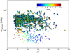 |
Fig. 5 Mean core rotational splitting as a function of the mixed-mode density measured through Eqs. (9) and (10). The colour code indicates the stellar mass estimated from the asteroseismic global parameters. Coloured triangles represent the measurements obtained in this study. Black crosses and coloured dots represent the measurements of Mosser et al. (2012b) for stars on the red giant branch and in the red clump, respectively. |
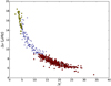 |
Fig. 6 Large separation as a function of the mixed-mode density for red giant branch stars where our method failed to propose a satisfactorily identification of the rotational components. Stars that have
|

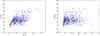 |
Fig. 7 Mass distribution of red giant branch stars where the rotational multiplet components have been identified. The darkness of the dots is positively correlated with the number of superimposed dots. Left panel: mass as a function of the radius. Right panel: mass as a function of the mixed-mode density. |
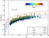 |
Fig. 8 Evolution of the radius as a function of the mixed-mode density on the red giant branch. Coloured triangles represent the measurements obtained in this study, the colour coding represents the mass estimated from the asteroseismic global parameters. Evolutionary tracks are computed with MESA for different masses. The coloured dots indicate the bottom of the RGB for the different masses. The vertical black dashed line indicates the lower observational limit for the mixed-mode density,
|

5.2 Investigating the core slow-down rate as a function of the stellar mass
On the one hand, Eggenberger et al. (2017) explored the influence of the stellar mass on the efficiency of the angular momentum transport, but they only considered two stars with different masses. On the other hand, the measurements of Mosser et al. (2012b) actually included a small number of stars on the RGB and the highest mass was around 1.7 M⊙, with only three high-mass stars. We now have a much larger dataset covering a broad mass range, from 1 up to 2.5 M⊙, allowing us to investigate how the mean core rotational splitting and the slow-down rate of the core rotation depend on the stellar parameters. We considered different mass ranges, chosen in order to ensure a sufficiently large number of stars in each mass interval. We then measured for each mass range the mean value of the core rotational splitting ⟨δνrot,core⟩ and investigated a relationship of the type
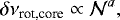 (26)
(26)
with the a values resulting from a non-linear least squares fit on each mass interval (Fig. 10). The measured ⟨δνrot,core⟩ and a values are summarized in Table 1 as a function of the mass range. The results indicate that the mean core rotational splittings and core rotation slow-down rate are the same, to the precision of our measurements, for all stellar mass ranges considered in this study (Table 1 and Fig. 11). Moreover, the mean slow-down rate measured in this study islower than what we derive when using all the Mosser et al. (2012b) measurements on the RGB (Table 2).
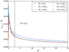 |
Fig. 9 Evolution of the relative position of the core boundary, namely the radius of the core normalized to the total stellar radius, as a function of the mixed-mode density
|

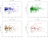 |
Fig. 10 Mean core rotational splitting as a function of the mixed-mode density for different mass ranges. Coloured triangles represent the measurements obtained in this study while grey crosses represent the measurements of Mosser et al. (2012b) on the red giant branch. The coloured lines represent the corresponding fits of the core slow-down obtained from Eq. (26). Upper left panel: M ≤ 1.4 M⊙. Upper right panel: 1.4 < M ≤ 1.6 M⊙. Lower left panel: 1.6 < M ≤ 1.9 M⊙. Lower right panel: M > 1.9 M⊙. |
6 Discussion
We selected the 57 RGB stars for which we and Mosser et al. (2012b) obtained mean core rotation measurements. We then considered either the radius or the mixed-mode density as a proxy of stellar evolution. In the following, we explore the origin of the discrepancy found between the mean slow-down rate of the core rotation measured in this work and the mean slope measured when using Mosser et al. (2012b) results. We then address the mass dependence of the core slow-down rate. We finally discuss the limitations and implications of our results.
6.1 Origin of the observed discrepancies
We first compared the slow-down rates obtained with our measurements and those of Mosser et al. (2012b) as a function of the radius (Fig. 12). The measured slopes strongly differ from each other, the slow-down rate we obtained with our measurements being lower (Table 3). The significant differences between these two sets of measurements arise from the two stars with a radius larger than 9.5 R⊙, for which Mosser et al. (2012b) underestimated the mean core rotational splittings. We checked that we recover slopes that are in agreement when excluding these stars from the two datasets.
We also made the same comparison using the mixed-mode density  as a proxy of stellar evolution (Fig. 13) and found slopes in agreement (Table 3). The smaller discrepancy comes from the redistribution of the repartition of δνrot,core measurements induced by
  , which probes the stellar evolutionary stage, compared to what is observed when using the radius. These slopes are in agreement but are significantly larger than what we derive from a sample ten times larger. The discrepancy thus comes from a sample effect. Hence, the sample of Mosser et al. (2012b) is somehow biased. This is not surprising because their method waslimited to simple cases, that is, to small splittings. This confusion limit is more likely reached when Δ ν decreases, which corresponds in average to more evolved stars. Thus, in the approach followed by Mosser et al. (2012b), it is easier to measure large splittings at low
  since they are working with frequency instead of stretched periods. On the contrary, when
  increases it is harder to measure large splittings because the rotational multiplet components are entangled. In these conditions, stars showing a non-ambiguous rotational signature are more likely to present low splittings. This deficit in large splittings at large
  tends to result in a negative slope, suggesting a slow-down of the core rotation. Working with stretched periods allows us to measure reliable splittings well beyond the confusion limit. Thus, our measurements, encompassing a much larger sample, allow us to refine the diagnosis of Mosser et al. (2012b) on the evolution of the core rotation along the RGB and to reveal that this evolution is independent of the stellar mass. They confirm low core-rotation rates on the low RGB, and indicate that the core rotation seems to remain constant on the part of the RGB covered by our sample, instead of slightly slowing down. This reinforces the need to find physical mechanisms to counterbalance the core contraction along the RGB, which should lead to an acceleration of the core rotation in the absence of angular momentum transport. Furthermore, models still need to reconcile with observations as they predict core rotation rates at least ten times higher than those measured.
Slow-down rates and mean core rotational splittings.
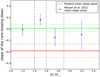 |
Fig. 11 Slopes of the core slow-down a when considering the evolution of the core rotation as a function of the mixed-mode density
|


Slow-down rates on the red giant branch.
6.2 Mass dependence of the core slow-down rate
Our results suggest a similar evolution of the core rotation for various masses on the red giant branch. This constitutes a striking feature and hopefully a fruitful indication in the search for the physical process at work. It is not in contradiction with the conclusion made by Eggenberger et al. (2017) that the efficiency of the angular momentum transport would increase with stellar mass, since a 2.5 M⊙ star evolves 100 times faster than a 1 M⊙ star on the RGB (Table 4). However, things are not so simple as the evolutionary timescale is not the only parameter at stake. More modelling work will be necessary to go from these measurements to quantitative estimates in terms of angular momentum transport and to bring tighter constraints on the mechanisms at work. This goes beyond the scope of the present work.
6.3 Mean core rotation
We must keep in mind that the measured δνrot,core are the rotational splittings of the most g-dominated dipole modes, which does not directly scale with the core rotation rate (Eqs. (12)–(14)). In practice, βcore∕βenv ≫ 1 only on the high RGB accessible with asteroseismology. On the lower RGB, the envelope contribution to the splittings of g-m modes is not negligible. We thus need to introduce a correction factor η into Eq. (17) to derive an accurate estimation of the mean core rotation rate (Mosser et al. 2012b) as
 (27)
(27)
with
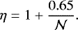 (28)
(28)
However, the relative deviation between  values derived with and without the η correction factor remains limited to around 15% in absolute value. In these conditions, δνrot,core can be used as a proxy of the red giant mean core rotation and provides clues on its evolution during the RGB stage. Moreover, the η correction is only a proxy for the correction of the envelope contribution. A complete interpretation in terms of the evolution of the red giant core rotation from the measured splittings requires the computation of rotational kernels, which is left to further studies.
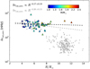 |
Fig. 12 Mean core rotational splitting as a function of the radius estimated from the global asteroseismic parameters. Our measurements are represented by coloured triangles, the colour code being the same as in Fig. 5. Mosser et al. (2012b)’s measurements on the RGB and on the clump are represented by grey crosses and dots, respectively. RGB stars are common to our study and to the Mosser et al. (2012b) study. The linear fit resulting from our RGB measurements is plotted in black while the fit resulting from Mosser et al. (2012b) RGB measurements is represented in grey. |
Slow-down rates on the RGB.
6.4 Implications for the high RGB and the clump
We must also keep in mind that asteroseismology allows us to probe stellar interiors for only a fraction of the time spent by stars on the RGB (tobs∕tRGB in Table 4). Thus, existing seismic measurements cannot bring constraints on the evolution of the core rotation on the high RGB, and we have to rely on modelling in this evolutionary stage. We know that a significant braking must occur in this evolutionary stage, unfortunately out of reach of seismic measurements. Indeed, compared to what we measure for RGB stars, the mean rotational splitting on the red clump is divided by a factor of eight for M ≤ 1.2 M⊙ stars and a factor of four for M > 1.9 M⊙ stars, as seen in Fig. 5.
Finally, the fact that  is a good proxy of stellar evolution on the RGB is not the case on the clump. Clump and RGB stars have mixed-mode densities located in the same range of values, which seems to indicate that
  decreases from the tip of the RGB (Fig. 5). This is confirmed by models computed with MESA, which indicate that
  strongly decreases when helium burning is firmly established in the core. Moreover, data emphasize that the dispersion of the
  values met in the clump rises from a mass effect and does not trace the stellar evolution in the clump (Fig. 5). Higher mass stars have lower
  values on average. This trend is confirmed by models that predict lower
  values on the clump when the stellar mass increases.
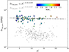 |
Fig. 13 Same as Fig. 12, this time representing the mean core rotational splitting as a function of the mixed-modedensity. |
Evolutionary timescales given by MESA for different stellar masses, either on the whole RGB (tRGB) and accessible through asteroseismology for  (tobs).
7 Conclusion
Mixed modes and splittings can now be disentangled in a simple and almost automated way through the use of stretched period spectra. This opens the era of large-scale measurements of the core rotation of red giants necessary to prepare the analysis of Plato data representing hundreds of thousands of potential red giants. We developed a method allowing an automatic identification of the dipole gravity-dominated mixed-modes split by rotation, providing us with a measurement of the mean core rotational splitting δνrot,core for red giant branch stars, even when mixed modes and splittings are entangled. As rotational components with different azimuthal orders are now well identified in the full power spectrum, we can now have access to large rotational splitting values in a simple way.
We obtained mean core rotation measurements for 875 red giant branch stars, covering a broad mass range from 1 to 2.5 M⊙. This led to the possibility of unveiling the role of the stellar mass in the core rotation slow-down rate. These measurements, obtained using a more elaborate method applied to a much larger sample, allowed us to extend the results of Mosser et al. (2012b) through a more precise characterization of the evolution of the mean core rotation on the red giant branch, and to unveil how this evolution depends on the stellar mass. As evolutionary sequences calculated with MESA for various stellar masses emphasized that the radius, used by Mosser et al. (2012b), is not a good proxy of stellar evolution, we used instead the mixed-mode density  . Our results are not in contradiction with the conclusions of Mosser et al. (2012b), as they confirm low core rotation rates on the low red giant branch and indicate that the core rotation is almost constant instead of slightly slowing down on the part of the RGB to which we have access. It also appeared that this rotation is independent of the mass and remains constant over the red giant branch encompassed by our observational set. This conclusion differs from previous results and is due to the combination of the use of a larger and less biased dataset. As stars in our sample evolve on the RGB with very different timescales, this result implies that the mechanisms transporting angular momentum should have different efficiencies for different stellar masses. Quantifying the efficiency of the angular momentum transport requires a deeper use of models. This is beyond the scope of this paper and left to further studies.
Acknowledgements
We acknowledge financial support from the Programme National de Physique Stellaire (CNRS/INSU). We thank Sébastien Deheuvels for fruitful discussions, and the entire Kepler team, whose efforts made these results possible.
References
- Angulo, C., Arnould, M., Rayet, M., et al. 1999, Nucl. Phys. A, 656, 3 [NASA ADS] [CrossRef] [Google Scholar]
- Beck, P. G., Bedding, T. R., Mosser, B., et al. 2011, Science, 332, 205 [NASA ADS] [CrossRef] [PubMed] [Google Scholar]
- Bedding, T. R., Mosser, B., Huber, D., et al. 2011, Nature, 471, 608 [NASA ADS] [CrossRef] [PubMed] [Google Scholar]
- Belkacem, K., Marques, J. P., Goupil, M. J., et al. 2015a, A&A, 579, A30 [NASA ADS] [CrossRef] [EDP Sciences] [Google Scholar]
- Belkacem, K., Marques, J. P., Goupil, M. J., et al. 2015b, A&A, 579, A31 [NASA ADS] [CrossRef] [EDP Sciences] [Google Scholar]
- Böhm-Vitense, E. 1958, Z. Astrophys., 46, 108 [Google Scholar]
- Cantiello, M., Mankovich, C., Bildsten, L., et al. 2014, ApJ, 788, 93 [NASA ADS] [CrossRef] [Google Scholar]
- Ceillier, T., Eggenberger, P., García, R. A., et al. 2013, A&A, 555, A54 [NASA ADS] [CrossRef] [EDP Sciences] [Google Scholar]
- Cox, J. P., & Giuli, R. T. 1968, Principles of Stellar Structure (New York: Gordon and Breach) [Google Scholar]
- Deheuvels, S., Doğan, G., Goupil, M. J., et al. 2014, A&A, 564, A27 [NASA ADS] [CrossRef] [EDP Sciences] [Google Scholar]
- De Ridder, J., Barban, C., Baudin, F., et al. 2009, Nature, 459, 398 [Google Scholar]
- Dupret, M.-A., Belkacem, K., Samadi, R., et al. 2009, A&A, 506, 57 [NASA ADS] [CrossRef] [EDP Sciences] [Google Scholar]
- Eggenberger, P., Montalbán, J., & Miglio, A. 2012, A&A, 544, L4 [NASA ADS] [CrossRef] [EDP Sciences] [Google Scholar]
- Eggenberger, P., Lagarde, N., Miglio, A., et al. 2017, A&A, 599, A18 [NASA ADS] [CrossRef] [EDP Sciences] [Google Scholar]
- Ferguson, J. W., Alexander, D. R., Allard, F., et al. 2005, ApJ, 623, 585 [NASA ADS] [CrossRef] [Google Scholar]
- Fuller, J., Lecoanet, D., Cantiello, M., et al. 2014, ApJ, 796, 17 [Google Scholar]
- Gehan, C., Mosser, B., & Michel, E. 2017, EPJ Web Conf., 160, 04005 [NASA ADS] [CrossRef] [EDP Sciences] [Google Scholar]
- Goupil, M. J., Mosser, B., Marques, J. P., et al. 2013, A&A, 549, A75 [NASA ADS] [CrossRef] [EDP Sciences] [Google Scholar]
- Grevesse, N., & Noels, A. 1993, Phys. Scr., T47, 133 [Google Scholar]
- Grosjean, M., Dupret, M.-A., Belkacem, K., et al. 2014, A&A, 572, A11 [NASA ADS] [CrossRef] [EDP Sciences] [Google Scholar]
- Hekker, S., & Christensen-Dalsgaard, J. 2017, A&ARv, 25, 1 [NASA ADS] [CrossRef] [EDP Sciences] [Google Scholar]
- Iglesias, C. A., & Rogers, F. J. 1996, ApJ, 464, 943 [NASA ADS] [CrossRef] [Google Scholar]
- Kallinger, T., Weiss, W. W., Barban, C., et al. 2010, A&A, 509, A77 [NASA ADS] [CrossRef] [EDP Sciences] [Google Scholar]
- Kjeldsen, H., & Bedding, T. R. 1995, A&A, 293, 87 [NASA ADS] [Google Scholar]
- Lagarde, N., Decressin, T., Charbonnel, C., et al. 2012, A&A, 543, A108 [NASA ADS] [CrossRef] [EDP Sciences] [Google Scholar]
- Lagarde, N., Bossini, D., Miglio, A., Vrard, M., & Mosser, B. 2016, MNRAS, 457, L59 [NASA ADS] [CrossRef] [Google Scholar]
- Ledoux, P. 1951, ApJ, 114, 373 [NASA ADS] [CrossRef] [Google Scholar]
- Marques, J. P., Goupil, M. J., Lebreton, Y., et al. 2013, A&A, 549, A74 [NASA ADS] [CrossRef] [EDP Sciences] [Google Scholar]
- Montalbán, J., Miglio, A., Noels, A., et al. 2013, ApJ, 766, 118 [NASA ADS] [CrossRef] [Google Scholar]
- Mosser, B., & Miglio, A. 2016, in The CoRot Legacy Book: The Adventure of the Ultra High Precision Photometry from space, ed. CoRot Team, 197 [Google Scholar]
- Mosser, B., Belkacem, K., Goupil, M. J., et al. 2011, A&A, 525, L9 [NASA ADS] [CrossRef] [EDP Sciences] [Google Scholar]
- Mosser, B., Elsworth, Y., Hekker, S., et al. 2012a, A&A, 537, A30 [NASA ADS] [CrossRef] [EDP Sciences] [Google Scholar]
- Mosser, B., Goupil, M. J., Belkacem, K., et al. 2012b, A&A, 548, A10 [NASA ADS] [CrossRef] [EDP Sciences] [Google Scholar]
- Mosser, B., Goupil, M. J., & Belkacem, K., et al. 2012c, A&A, 540, A143 [NASA ADS] [CrossRef] [EDP Sciences] [Google Scholar]
- Mosser, B., Michel, E., Belkacem, K., et al. 2013, A&A, 550, A126 [NASA ADS] [CrossRef] [EDP Sciences] [Google Scholar]
- Mosser, B., Benomar, O., & Belkacem, K., et al. 2014, A&A, 572, L5 [NASA ADS] [CrossRef] [EDP Sciences] [PubMed] [Google Scholar]
- Mosser, B., Vrard, M., Belkacem, K., et al. 2015, A&A, 584, A50 [NASA ADS] [CrossRef] [EDP Sciences] [Google Scholar]
- Mosser, B., Belkacem, K., Pinçon, C., et al. 2017, A&A, 598, A62 [NASA ADS] [CrossRef] [EDP Sciences] [Google Scholar]
- Ouazzani, R.-M., Goupil, M. J., Dupret, M.-A., & Marques, J. P. 2013, A&A, 554, A80 [NASA ADS] [CrossRef] [EDP Sciences] [Google Scholar]
- Paxton, B., Bildsten, L., Dotter, A., et al. 2011, ApJS, 192, 3 [Google Scholar]
- Paxton, B., Cantiello, M., Arras, P., et al. 2013, ApJS, 208, 4 [NASA ADS] [CrossRef] [Google Scholar]
- Paxton, B., Marchant, P., Schwab, J., et al. 2015, ApJS, 220, 15 [Google Scholar]
- Pinçon, C., Belkacem, K., Goupil, M. J., & Marques, J. P. 2017, A&A, 605, A31 [NASA ADS] [CrossRef] [EDP Sciences] [Google Scholar]
- Pinsonneault, M. H., Elsworth, Y., Epstein, C., et al. 2014, ApJS, 215, 19 [NASA ADS] [CrossRef] [Google Scholar]
- Rogers, F. J., & Nayfonov, A. 2002, ApJ, 576, 1064 [Google Scholar]
- Rüdiger, G., Gellert, M., Spada, F., & Tereshin, I. 2015, A&A, 573, A80 [NASA ADS] [CrossRef] [EDP Sciences] [Google Scholar]
- Scuflaire, R. 1974, A&A, 36, 107 [NASA ADS] [Google Scholar]
- Spada, F., Gellert, M., Arlt, R., et al. 2016, A&A, 589, A23 [NASA ADS] [CrossRef] [EDP Sciences] [Google Scholar]
- Stello, D., Huber, D., Bedding, T. R., et al. 2013, ApJ, 765, L41 [NASA ADS] [CrossRef] [Google Scholar]
- Talon, S., & Zahn, J.-P. 1997, A&A, 317, 749 [Google Scholar]
- Unno, W., Osaki, Y., Ando, H., Saio, H., & Shibahashi, H. 1989, Nonradial Oscillations of Stars (Tokyo: University of Tokyo Press) [Google Scholar]
- Vrard, M., Mosser, B., Samadi, R., et al. 2016, A&A, 588, A87 [NASA ADS] [CrossRef] [EDP Sciences] [Google Scholar]
- Vrard, M., Mosser, B., & Barban, C. 2017, EPJ Web Conf., 160, 04012 [Google Scholar]
- Zahn, J.-P. 1992, A&A, 265, 115 [NASA ADS] [Google Scholar]
All Tables
Evolutionary timescales given by MESA for different stellar masses, either on the whole RGB (tRGB) and accessible through asteroseismology for (tobs).
All Figures
|
Fig. 1 Stretching function ζ (blue line) computed with Δν = 11 μHz, Δ Π1 = 80 s, and q = 0.12. The asymptotic behaviours of ζ for g-m and p-m modes are indicated by a red and green line, respectively. |
| In the text | |
|
Fig. 2 Stretched period échelle diagrams for red giant branch stars with different inclinations. The rotational components are identified in an automatic way through a correlation of the observed spectrum with a synthetic one constructed using Eq. (9). The colours indicate the azimuthal order: the m = {−1, 0, +1} rotationalcomponents are represented in green, light blue, and red, respectively. The symbol size varies as the power spectral density. Left panel: star seen pole-on where only the m = 0 rotational component is visible. Middle panel: star seen equator-on where the m = {−1, +1} componentsare visible. Right panel: star with an intermediate inclination angle where all the three components are visible. |
| In the text | |
|
Fig. 3 Synthetic stretched period échelle diagram built from Eqs. (9) and (10). The colours indicate the azimuthal order: the m = {−1, 0, +1} rotational components are given by green triangles, blue dots, and red crosses, respectively. The small black dots represent
|
| In the text | |
|
Fig. 4 Comparison of the present results with those from Mosser et al. (2012b) for stars on the red giant branch. The solid red line represents the 1:1 relation. The red dashed lines represent the 1:2 and 2:1 relations. |
| In the text | |
|
Fig. 5 Mean core rotational splitting as a function of the mixed-mode density measured through Eqs. (9) and (10). The colour code indicates the stellar mass estimated from the asteroseismic global parameters. Coloured triangles represent the measurements obtained in this study. Black crosses and coloured dots represent the measurements of Mosser et al. (2012b) for stars on the red giant branch and in the red clump, respectively. |
| In the text | |
|
Fig. 6 Large separation as a function of the mixed-mode density for red giant branch stars where our method failed to propose a satisfactorily identification of the rotational components. Stars that have
|
| In the text | |
|
Fig. 7 Mass distribution of red giant branch stars where the rotational multiplet components have been identified. The darkness of the dots is positively correlated with the number of superimposed dots. Left panel: mass as a function of the radius. Right panel: mass as a function of the mixed-mode density. |
| In the text | |
|
Fig. 8 Evolution of the radius as a function of the mixed-mode density on the red giant branch. Coloured triangles represent the measurements obtained in this study, the colour coding represents the mass estimated from the asteroseismic global parameters. Evolutionary tracks are computed with MESA for different masses. The coloured dots indicate the bottom of the RGB for the different masses. The vertical black dashed line indicates the lower observational limit for the mixed-mode density,
|
| In the text | |
|
Fig. 9 Evolution of the relative position of the core boundary, namely the radius of the core normalized to the total stellar radius, as a function of the mixed-mode density
|
| In the text | |
|
Fig. 10 Mean core rotational splitting as a function of the mixed-mode density for different mass ranges. Coloured triangles represent the measurements obtained in this study while grey crosses represent the measurements of Mosser et al. (2012b) on the red giant branch. The coloured lines represent the corresponding fits of the core slow-down obtained from Eq. (26). Upper left panel: M ≤ 1.4 M⊙. Upper right panel: 1.4 < M ≤ 1.6 M⊙. Lower left panel: 1.6 < M ≤ 1.9 M⊙. Lower right panel: M > 1.9 M⊙. |
| In the text | |
|
Fig. 11 Slopes of the core slow-down a when considering the evolution of the core rotation as a function of the mixed-mode density
|
| In the text | |
|
Fig. 12 Mean core rotational splitting as a function of the radius estimated from the global asteroseismic parameters. Our measurements are represented by coloured triangles, the colour code being the same as in Fig. 5. Mosser et al. (2012b)’s measurements on the RGB and on the clump are represented by grey crosses and dots, respectively. RGB stars are common to our study and to the Mosser et al. (2012b) study. The linear fit resulting from our RGB measurements is plotted in black while the fit resulting from Mosser et al. (2012b) RGB measurements is represented in grey. |
| In the text | |
|
Fig. 13 Same as Fig. 12, this time representing the mean core rotational splitting as a function of the mixed-modedensity. |
| In the text | |
Current usage metrics show cumulative count of Article Views (full-text article views including HTML views, PDF and ePub downloads, according to the available data) and Abstracts Views on Vision4Press platform.
Data correspond to usage on the plateform after 2015. The current usage metrics is available 48-96 hours after online publication and is updated daily on week days.
Initial download of the metrics may take a while.