| Issue |
A&A
Volume 650, June 2021
|
|
|---|---|---|
| Article Number | A116 | |
| Number of page(s) | 27 | |
| Section | Planets and planetary systems | |
| DOI | https://doi.org/10.1051/0004-6361/202039210 | |
| Published online | 15 June 2021 | |
N-body simulations of planet formation via pebble accretion
II. How various giant planets form
1
School of Engineering, Physics, and Mathematics, University of Dundee,
Dundee
DD1 4HN, UK
e-mail: s.matsumura@dundee.ac.uk
2
Earth-Life Science Institute, Tokyo Institute of Technology,
Meguro-ku,
Tokyo
152-8550, Japan
Received:
18
August
2020
Accepted:
15
February
2021
Aims. The connection between initial disc conditions and final orbital and physical properties of planets is not well-understood. In this paper, we numerically study the formation of planetary systems via pebble accretion and investigate the effects of disc properties such as masses, dissipation timescales, and metallicities on planet formation outcomes.
Methods. We improved the N-body code SyMBA that was modified for our Paper I by taking account of new planet–disc interaction models and type II migration. We adopted the ‘two-α’ disc model to mimic the effects of both the standard disc turbulence and the mass accretion driven by the magnetic disc wind.
Results. We successfully reproduced the overall distribution trends of semi-major axes, eccentricities, and planetary masses of extrasolar giant planets. There are two types of giant planet formation trends, depending on whether or not the disc’s dissipation timescales are comparable to the planet formation timescales. When planet formation happens fast enough, giant planets are fully grown (Jupiter mass or higher) and are distributed widely across the disc. On the other hand, when planet formation is limited by the disc’s dissipation, discs generally form low-mass cold Jupiters. Our simulations also naturally explain why hot Jupiters (HJs) tend to be alone and how the observed eccentricity-metallicity trends arise. The low-metallicity discs tend to form nearly circular and coplanar HJs in situ, because planet formation is slower than high-metallicity discs, and thus protoplanetary cores migrate significantly before gas accretion. The high-metallicity discs, on the other hand, generate HJs in situ or via tidal circularisation of eccentric orbits. Both pathways usually involve dynamical instabilities, and thus HJs tend to have broader eccentricity and inclination distributions. When giant planets with very wide orbits (“super-cold Jupiters”) are formed via pebble accretion followed by scattering, we predict that they belong to metal-rich stars, have eccentric orbits, and tend to have (~80%) companions interior to their orbits.
Key words: planets and satellites: general / planets and satellites: formation / protoplanetary disks / methods: numerical
© ESO 2021
1 Introduction
Accretion of both pebbles and planetesimals is likely to contribute to planet formation (e.g. Ida et al. 2016; Johansen & Lambrechts 2017). The pebbles are cm- to m-sized particles, which are very sensitive to gas drag (Adachi et al. 1976; Weidenschilling 1977). Since their migration timescale is short compared to the growth timescale (Birnstiel et al. 2012; Lambrechts & Johansen 2014), they are expected to rapidly migrate towards the central star without much growth. These migrating dust particles could be concentrated to form 100–1000 km-sized planetesimals directly (which correspond to ~ 10−6 –10−4 M⊕) (e.g. Johansen et al. 2015; Simon et al. 2016), either via the trapping of dust grains in pressure bumps of the protoplanetary disc or via streaming instability (Youdin & Goodman 2005; Johansen et al. 2007, 2009). These planetesimals are initially likely to grow via planetesimal–planetesimal collisions (Ida et al. 2016; Johansen & Lambrechts 2017), until the protoplanetary cores become massive enough to have a large capturing radius of pebbles comparable to the Hill radius (Ormel & Klahr 2010; Kretke & Levison 2014). The stage of a protoplanetary core growth via pebbles is called “pebble accretion”. The pebble accretion slows down when the capturing radius becomes larger than the pebble-disc scale height, and thus the accretion becomes two-dimensional. At such a stage, both pebble and planetesimal accretion may contribute to mass growth (e.g. Ida et al. 2016).
Ormel & Klahr (2010) first developed the analytical model of particle-protoplanet interactions in a gas disc, and pointed out the efficiency of pebble accretion in the settling regime where gas drag effects are significant. The pebble accretion was further studied by considering the growth of a single core (Bitsch et al. 2015) and by using sophisticated N-body simulations (Levison et al. 2015; Chambers 2016). All of these studies confirmed the efficiency of pebble accretion and showed that a variety of planetary systems could be formed within a typical gas disc lifetime. However, the model by Bitsch et al. (2015) was not designed to assess the planet-planet interaction effects, which are important to determine the final orbital architecture of planetary systems. The models by Levison et al. (2015) and Chambers (2016) focused on the detailed physics of growth and destruction of particles ranging from pebbles to planets, and did not take account of planet migration effects, which are also important to determine the orbital distribution of planets.
Matsumura et al. (2017, Paper I) implemented the analytical pebble accretion model by Ida et al. (2016) into an N-body code SyMBA (Duncan et al. 1998), and performed global N-body simulations of pebble accretion over a range of disc parameters. Although the work has confirmed that pebble accretion leads to a variety of planetary systems, it failed to reproduce the overall distribution trends of the physical and orbital parameters of extrasolar giant planets. In particular, few giant planets were formed, because most planetary cores were lost to the disc’s inner edge due to migration, in a similar manner to planetesimal accretion simulations (e.g. Coleman & Nelson 2016b). The problem was that a range of planetary masses leading to outward migration (Paardekooper et al. 2011) is very narrow, so growing planets eventually start migrating inward (also see Brasser et al. 2017). Therefore, although pebble accretion may be more efficient compared to planetesimal accretion (e.g. Lambrechts & Johansen 2012; Kretke & Levison 2014), the giant planet formation timescale still appeared to be too long compared to the migration timescale, and thus the migration problem remained.
There has been a significant development regarding the formation of ‘cold’ giant planets (i.e. Jupiter-like planets beyond ~1 au) in the past few years. The formation of such planets has been particularly difficult largely because of the efficient migration of protoplanetary cores discussed above (e.g. Coleman & Nelson 2016b; Matsumura et al. 2017). Bitsch et al. (2015) mitigated the issue and successfully formed cold Jupiters (CJs) by placing cores far from the central star (beyond ~15 au) in an evolved disc (up to ~2 Myr) with a relatively short disc lifetime of 3 Myr. Coleman & Nelson (2016a) resolved the migration issue by considering the temporal planet ‘traps’ due to variations in the effective viscous stresses. More recently, Ida et al. (2018) proposed an elegant solution by combining two recent key developments in the field — the new type II migration formula (Kanagawa et al. 2018) and the wind-driven accretion disc with the nearly laminar interior (e.g. Bai & Stone 2013; Bai 2017), where both contribute to slowing down type II migration and make the formation of CJs possible.
One of these key developments comes from the realisation that the migration of a gap-opening planet is not tied to the disc evolution. This is because, differently from the assumption of the classical type II migration model (Lin & Papaloizou 1986, 1993), the disc gas proved to cross the gap opened by a planet. The new type II migration formula by Kanagawa et al. (2018) reflects the results of recent hydrodynamic simulations (Duffell & MacFadyen 2013; Fung et al. 2014) as well as their own, and shows that the migration is slower for a planet with the deeper gap (i.e. for a smaller viscosity disc, a lower disc temperature, or a larger mass planet, also see Eq. (8)). Compared to the classical type II formula, the new formula typically gives ~ 1 order of magnitude longer migration timescales (Ida et al. 2018).
The other key development is the accretion mechanism of a protoplanetary disc. In the classical picture, the disc’s viscosity drives the angular momentum transfer in the protoplanetary disc, and the chief explanation for the viscosity is the magnetorotational instability turbulence (e.g. Balbus & Hawley 1998). Recent non-ideal magnetohydrodynamic simulations, however, have shown that the protoplanetary discs are likely to be largely laminar due to the combined effects of ambipolar diffusion, Hall effects and Ohmic dissipation, and the fact that the disc’s angular momentum is mostly removed by the magnetic disc wind (e.g. Bai & Stone 2013; Bai 2017). Following this idea, Ida et al. (2018) adopted two different alphas: one representing the disc accretion driven by the mass loss due to the magnetic disc wind αacc, and the other representing the local disc turbulence αturb. Since the gap opening is controlled by the disc turbulence and since the turbulence is expected to be very weak αturb ≲ 10−4 (e.g. Bai 2017), the estimated type II migration is slower than it is using the α required to explain the observed stellar mass accretion rate (α ~ 10−2 in Hartmann et al. 1998, see Sect. 2.2 as well). A similar study was conducted by Wimarsson et al. (2020) using N-body simulations with pebble accretion. Besides the new type II mechanism described above, they show that the transition zone between viscously and radiatively heated disc regions could work as a temporal planet trap and promote more efficient planetary growth via collisions.
Recently, a trilogy of papers on N-body pebble accretion simulations was published, with two of them exploring the formation of super-Earths (SEs) or lower mass planets (Lambrechts et al. 2019; Izidoro et al. 2021), and the other focusing on the formation of giant planets (Bitsch et al. 2019). For SEs and lower mass planets, they proposed that Earth-like planets were formed in the low pebble flux disc with little migration, while SE-like planets were formed in the higher pebble flux disc. In the latter case, their growing cores migrated to the disc’s inner edge in a similar manner to Matsumura et al. (2017), but these cores were more efficiently trapped in mean-motion resonances (MMRs) because they chose the disc dissipation timescale comparable to the migration timescale so that the migration would be halted completely near the inner edge of the disc. As a result, their protoplanets became dynamically unstable as the gas disc dissipated and the protoplanets collided with one another and formed non-resonant multiple SEs (cf. Ogihara et al. 2010). However, the disc-planet interactions near the disc edge is not well understood, and the planet trapping efficiency depends on the sharpness of the disc edge (Ogihara et al. 2010) and the details of the torque balance (Brasser et al. 2018). For giant planets, on the other hand, Bitsch et al. (2019) compared the classical α disc model with α = 5.3 × 10⁻³ with a “two-α” disc model similar to that of Ida et al. (2018) with αacc = 5.3 × 10⁻³ and αturb = 5.3 × 10⁻⁴–10−4, and successfully produced CJs. However, they failed to form highly eccentric giant planets (see discussion in Sect. 4.7).
The goal of this work, like that of our previous work (Matsumura et al. 2017), is to investigate how initial disc conditions are related to physical and orbital properties of planets by comparing planetary systems formed via numerical simulations with observed extrasolar planetary systems. This kind of study of connecting planetary systems with protoplanetary discs is becoming increasingly important. ALMA observations now regularly find gaps, spirals, and asymmetries in protoplanetary discs, which may be attributed to planet formation processes or forming planets (e.g. Andrews et al. 2018; Huang et al. 2018). There are also potential planetary candidates discovered in protoplanetary discs including PDS 70 (Keppler et al. 2018), HD 100546 (Brittain et al. 2019; Casassus & Pérez 2019), and TW Hya (Tsukagoshi et al. 2019). The future observations would allow us to further constrain planet formation processes occurring in protoplanetary discs.
As described in Sect. 2, we started with disc conditions motivated by observations, follow planet formation and orbital evolution by using an N-body code SyMBA (Duncan et al. 1998), and compare distributions of orbital and physical properties of simulated planets with those of observed ones. From this point of view, giant planets are particularly useful, because they are observed over a wide range of orbital radii, from less than 0.01 au to over 100 au. Super-Earths and lower-mass planets, on the other hand, are more abundant but are limited to the inner disc region (≲ 1 au). Therefore, in this paper, we pay particular attention to disc conditions that lead to different types of giant planets, ranging from close-in hot Jupiters to very distant super-cold Jupiters, though numerical simulations will generate all kinds of planets.
In Sect. 2, we introduce the numerical methods we used by highlighting the changes made since Matsumura et al. (2017). We improve the N-body code SyMBA (Duncan et al. 1998) by adopting a more self-consistent disc model and by taking account of recent developments of the field. In Sect. 3, we show that our numerical simulations reproduce overall trends of distributions of semi-major axis a, eccentricity e, and mass Mp of extrasolar giant planets. We describe the effects of different parameters on planet formation and also show how different types of giant planets (such as HJs and CJs) are formed. We discuss the results further in Sect. 4, and summarise our findings in Sect. 5.
2 Methods
We ran all of the simulations with the N-body integrator SyMBA (Duncan et al. 1998), which was modified to include models of planet formation, disc-planet interactions,and disc evolution. In this section, we highlight the updates made since Matsumura et al. (2017).
In Sect. 2.1, we introduce the planet–disc interaction model adopted from Ida et al. (2020), and we show how planet migration as well as eccentricity and inclination damping of protoplanetary orbits are modelled in our code. We also updated the type II migration prescription by following Kanagawa et al. (2018). In Sect. 2.2, we introduce planet formation and disc evolution models. We adopted the α disc model (Shakura & Sunyaev 1973), but we modified it to take account of a recent development in the field. Finally, in Sect. 2.3, we present the initial conditions of our simulations, and show a simple example of planet formation based on the prescriptions introduced in this section.
2.1 Orbital evolution of protoplanets
The orbital evolution of protoplanets is largely determined by their interactions with the gas disc. However, there are a few different definitions of the equation of motion used in the planetary literature. The difference is not only confusing but could lead to very different dynamical outcomes (e.g. Ida et al. 2020; Matsumura et al. 2017). Recently, Ida et al. (2020) compared a few such equations in the literature and highlighted which equations are appropriate under which conditions. Based on this work, we will use a new, more appropriate equation of motion.
In Matsumura et al. (2017), we adopted the equation proposed by Coleman & Nelson (2014):
 (1)
(1)
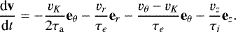
but we replaced the ‘migration timescale’  in the first term with the semi-major axis evolution timescale τa = −ȧ∕a. The motivation behind replacing τm with τa in Matsumura et al. (2017) was to avoid an artificial outward migration at the high eccentricity, supersonic regime. Here, vK,a and ΩK,a are the Keplerian orbital speed and the corresponding angular speed evaluated at the semi-major axis a, while v is the planetary velocity evaluated at the instantaneous orbital radius r, with vr, vθ, and vz being its polar coordinate components defined with the unit vectors er, eθ, and ez, respectively. Ida et al. (2020) showed that the azimuthal component of eccentricity damping is implicitly included in the first term of Eq. (1),
  , and its explicit addition as the second term is not necessary.
In this work, we adopted the equation of motion proposed by Ida et al. (2020), since the equation describes planet–disc interactions well both in subsonic and supersonic regimes compared to the other equations proposed so far. They introduced an intuitive model of planet–disc interactions based on dynamical friction by combining the work of Muto et al. (2011) in the supersonic regime with that of Tanaka & Ward (2004) in the subsonic regime. The equation reads as follows:
 (2)
(2)
We notethat vK is the Keplerian orbital speed evaluated at the instantaneous orbital radius r. In this model, the evolution timescales for the semi-major axis, eccentricity, and inclination are expressed as follows:
![\begin{align} \tau_{\textrm{a}} \,{=}\, & {-}\frac{t_{\textrm{wave}}}{2h_{\textrm{g}}^{2}}\left[\frac{\Gamma_{L}}{\Gamma_{0}}\left(1-\frac{1}{\pi}\frac{\Gamma_{L}}{\Gamma_{0}}\sqrt{\hat{e}^{2}+\hat{i}^{2}}\right)^{-1} \right. \nonumber \\ &\left.+\frac{\Gamma_{C}}{\Gamma_{0}}\exp\left(-\frac{\sqrt{e^{2}+i^{2}}}{e_{f}}\right)\right]^{-1},\\ \tau_{e} \,{=}\, & \frac{t_{\textrm{wave}}}{0.780}\,\left(1+\frac{1}{15}\left(\hat{e}^{2}+\hat{i}^{2}\right)^{3/2}\right),\\ \tau_{i} \,{=}\, & \frac{t_{\textrm{wave}}}{0.544}\,\left(1+\frac{1}{21.5}\left(\hat{e}^{2}+\hat{i}^{2}\right)^{3/2}\right),\end{align}](/articles/aa/full_html/2021/06/aa39210-20/aa39210-20-eq5.png)
where hg = Hg∕a is the gas disc’s aspect ratio, and eccentricities and inclinations scaled with hg are defined as ê = e∕hg and î = i∕hg, respectively. The exponential factor in τa is introduced with ef = 0.01 + hg∕2 following Fendyke & Nelson (2014), so that the contribution from the corotation torque disappears in the supersonic regime. Also, Γ∕Γ0 represents a normalised torque, and the subscripts L and C respectively correspond to Lindblad and corotation torques from Paardekooper et al. (2011), with the normalisation torque being
 (6)
(6)
Finally, twave is the characteristic time of the orbital evolution by Tanaka & Ward (2004):
 (7)
(7)
where Mp and M* are planetary and stellar masses, respectively, and Σg is the gas disc’s surface mass density. We note that twave is defined by using the semi-major axis a, not the instantaneous orbital radius r, so the timescales defined in Eqs. (3)–(5) are orbit-averaged timescales.
The above equations only hold for fully embedded type I migrators and need to be modified for gap-opening type II migrators. For planet migration, Kanagawa et al. (2018) have that type II migration is merely type I migration with the reduced surface mass density in the gap, and showed that such migration is well described by the following equation:
 (8)
(8)
where  . Since there is no consensus on eccentricity and inclination damping in the type II regime, we adjusted eccentricity and inclination damping timescales in a similar manner (
 and
and  ) and implemented the equation of motion (2) with timescales replaced by
  ,
,  , and
, and  in our code. In this prescription, the eccentricity and inclination damping timescales are always short compared to the migration timescale. This is an important condition for the “eccentricity trap” (Ogihara et al. 2010), where planets can be resonantly trapped near the disc’s inner edge. The condition also avoids spurious outward migration at the disc’s edge.
Figure 1 shows these timescales as a function of a protoplanetary mass for a circular and coplanar case. The vertical line indicates a critical mass Mcrit above whichplanet migration switches from type I to type II regimes, and it is defined as the mass having the minimum timescale of Eq. (8):
![\begin{eqnarray*} M_{\textrm{crit}} & = & \left[\frac{1}{0.04}\alpha_{\textrm{turb}}\left(\frac{H_{\textrm{g}}}{a}\right)^{5}\right]^{1/2}M_{*} \\ &\simeq\!& 9.3\left(\frac{\alpha_{\textrm{turb}}}{10^{-4}}\right)^{1/2}\left(\frac{H/a}{0.05}\right)^{5/2}\left(\frac{M_{*}}{M_{\odot}}\right)\;M_{\oplus}.\end{eqnarray*}](/articles/aa/full_html/2021/06/aa39210-20/aa39210-20-eq15.png)
Since this critical mass gives  and thus
  , the transition occurs when the gap depth is 50% of the nominal surface mass density (also see Johansen et al. 2019). The transition mass is sensitive to the disc’s aspect ratio, and we have Mcrit = 2.6 M⊕ for
  , αturb = 10−4, and M* = M⊙.
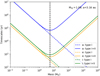 |
Fig. 1 Comparison of evolution timescales of semi-major axis τa (blue), eccentricity τe (orange), and inclination τi (green) for a planet at 3.16 au with the circular and coplanar orbit in Disc 6. Solid and dashed blue lines are from Eqs. (8) and (3), respectively. The vertical black dashed line indicates where migration timescale takes the minimum value (Eq. (10)). |
2.2 Planet formation and disc evolution
The mass growth rate of a protoplanet Ṁp is written asfollows:
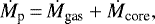 (11)
(11)
where Ṁgas and Ṁcore represent gas and coreaccretion rates of protoplanets, respectively. In this study, we assume that a protoplanetary core grows via pebble accretion and mutual collisions among themselves, and we do not take the effect of planetesimal accretion into account. This choice is justified when the pebble accretion is 3D (i.e. when the impact radius of a core is small compared to the scale height of the pebble disc b < hp), because the timescale of 3D pebble accretion is much shorter than that of the planetesimal accretion of the oligarchic growth stage (Ida et al. 2016). The pebble and planetesimal accretion timescales may become comparable to each other once the impact parameter of the core becomes larger than the pebble disc’s scale height b ≫ hp (Ida et al. 2016).
The core growth rate via pebble accretion is written as
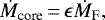 (12)
(12)
by using the accretion efficiency ϵ and the pebble mass flux ṀF. In the following, we describe the model of the stellar mass accretion rate Ṁ* and how ṀF is related to it. We also discuss the choice of pebble accretion efficiencies, and the pebble isolation masses. Finally, we present the model of the gas accretion rate onto a protoplanetary core Ṁgas.
2.2.1 Stellar mass flux Ṁ*
The evolution of a gas disc is represented by the stellar mass flux Ṁ*, which is also related to the evolution of a dust disc ṀF as it is discussed in the following sub-section. In this work, we used the same disc model as Matsumura et al. (2017), which is adopted from Ida et al. (2016). The disc’s midplane temperature T and the gas surface mass density Σg are modelled as the power-law functions of the orbital radius r as T ∝ r−q and Σg ∝r−p. Since the inner disc is heated by viscous dissipation while the outer disc is heated by the irradiation from the central star (e.g. Hueso & Guillot 2005; Oka et al. 2011), both T and Σg are dual power-law functions in our disc model.
The disc evolution is described by the diffusion equation for the disc’s surface mass density Σg :
![\begin{equation*}\frac{\partial\Sigma_{\textrm{g}}}{\partial t}\,{=}\,{-}\frac{1}{r}\frac{\partial}{\partial r}\left[3r^{1/2}\frac{\partial}{\partial r}\left(\Sigma_{\textrm{g}}\nu r^{1/2}\right)\right], \end{equation*}](/articles/aa/full_html/2021/06/aa39210-20/aa39210-20-eq21.png) (13)
(13)
where ν = αacccsH is the disc’s ‘viscosity’ representing the accretion. Assuming that the accretion is steady and that the effective viscosity is written as a power-law function in radius as ν ∝ rp (Lynden-Bell & Pringle 1974; Hartmann et al. 1998), the mass accretion rate is related to the surface mass density as follows:
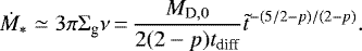 (14)
(14)
Here, MD,0 is the initial disc mass,  with the diffusion timescale of
 (15)
(15)
where rD is the characteristic disc size and νD is the corresponding viscosity.
As can be seen from the equation, there are several parameters we could use to specify the disc evolution, such as initial values of Ṁ*, MD, and Σg,D; as well as rD, αacc, and tdiff. However, they are dependent on one another, and we need to choose three parameters out of these to specify a disc model. For example, Ida & Lin (2008) chose MD,0, tdiff, and αacc as control parameters since they are relevant to planetesimal accretion as well as gap-opening criteria. For pebble accretion, however, the disc radius rD is important because the pebble mass flux decreases sharply once the pebble formation front reaches the outer disc radius (e.g. Sato et al. 2016). In this work, we considered a few different sets of MD,0 and tdiff, along with rD = 100 au. The choice of the characteristic disc size is rather arbitrary, but it is motivated by a typical size of observed protoplanetary discs (e.g. Andrews et al. 2010; Andrews & Williams 2007; Vicente & Alves 2005). The αacc is calculated from these values as follows:
 (16)
(16)
where hD = HD∕rD is the disc’s aspect ratio at rD, and torb,D is the corresponding orbital period. In Matsumura et al. (2017), we defined the stellar mass accretion rate and the alpha parameter independently of each other and calculated the surface mass density based on these parameters and the disc temperature models in Ida et al. (2016). In this work, we instead calculated the stellar mass accretion rate for given disc masses and diffusion timescales (and thus αacc), and we used these with the temperature model to determine the surface mass density profile. In this sense, our current disc model is more self-consistent compared to the previous one.
As discussed in Sect. 1, recent studies showed that disc accretion is driven by the magnetic disc wind rather than by the MRI turbulence (e.g. Bai & Stone 2013; Bai 2017). The follow-up studies proposed to replace the classical α disc model with the one incorporating the disc wind (Bai 2016; Suzuki et al. 2016), and the model has been adopted by N-body studies such as Ogihara et al. (2017). Some other works, on the other hand, opt to use two-α disc models by representing the mass accretion driven mainly by the disc wind, and the local disc evolution driven by turbulence with two different alphas (e.g. Ida et al. 2018; Johansen et al. 2019; Bitsch et al. 2019). In this work, we also adopted this two-α disc model for simplicity, and we represent the wind-driven disc accretion with αacc and the disc turbulence with αturb. Compared to the sophisticated wind-driven accretion models by Bai (2016) and Suzuki et al. (2016), this corresponds to approximating the combined effects of the wind-driven and turbulence-driven accretions with a single effective αacc, and ignoring the effect of the wind mass loss.
Finally, to choose our disc models, we constrained the combination of  by using the observed stellar mass accretion rates. Figure 2 shows eight disc models using Eq. (14), along with the observed stellar mass accretion rates from Sicilia-Aguilar et al. (2010) (data courtesy of Sicilia-Aguilar)1. Here, we didnot attempt to find the best fit to all the data, as this was done in Hartmann et al. (1998), but instead we tried to find a set of reasonable
  that makes Ṁ* go through at least some part of the distribution of observed accretion rates. This is because, as Hartmann et al. (1998) pointed out,the best fit to all data does not necessarily represent a typical evolution of the stellar mass accretion rates.
As can be seen in the figure, our chosen disc models tend to have long lifetimes. Towards the oldest ages (about a few to several tens of Myr), the mass accretion rate data are likely dominated by long-lived, potentially less common protoplanetary discs. However, a recent study shows that ~30% of stars mayhave disc lifetimes longer than 10 Myr (Pfalzner et al. 2014), making it possible that these long-lived discs may not be so uncommon. Therefore, in this work, we consider a relatively wide range of disc lifetimes. The combination of  and the corresponding αacc for eight disc models are summarised in Table 1. To mimic the photoevaporation effect, we reduced the mass accretion rate exponentially once it became lower than the critical value of 10−9 M⊙ yr−1. The choice of this critical value is arbitrary, but we chose it to be close to the minimum observed mass accretion rate seen in the figure. We note that, as seen in the table, αacc defined with our choices of parameters (tdiff = 0.1–10 Myr and rD = 100 AU) is higher than our default turbulent viscosity alpha value of αturb = 10−4, which is consistent with our assumption that the mass accretion is dominated by the disc’s wind effects. In Sect. 3.2.1, we discuss the effects of other values of αturb.
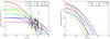 |
Fig. 2 Left: Stellar mass accretion rates Ṁ* for disc models 1–8 from Table 1 (Eq. (14)). The accretion is exponentially reduced after the critical mass accretion rate of 10−9 M⊙ yr−1 is reached (dashed lines). The black circles with error bars are observed stellar accretion rates from Sicilia-Aguilar et al. (2010) (data courtesy of Sicilia-Aguilar). Right: corresponding pebble mass fluxes ṀF (Eq. (25)). |
2.2.2 Pebble mass flux ṀF
To determine the pebble accretion rate by a protoplanet, we need to estimate the pebble mass flux. Lambrechts & Johansen (2014) wrote the pebble mass flux as follows:
 (17)
(17)
which describes the pebble mass swept up by the pebble formation front per unit time. Here, rpf is the radius of the pebble formation front, and Σp is the pebble surface mass density. Since the dust particles are likely to convert to pebbles over a long period of time, the dust surface mass density Σd should be different from that of pebbles Σp. At the pebble formation front, however, we assume Σd = Σp so that all dust particles are converted to pebbles there.
Another effect we need to take into account is that the pebble mass flux decreases drastically once the pebble formation front reaches the outer disc radius (e.g. Sato et al. 2016). Ida et al. (2019) fitted the numerical simulations by Sato et al. (2016) and proposed the following relation:
 (18)
(18)
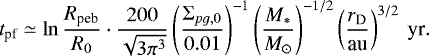
where Σpg = Σp∕Σg, the subscript 0 indicates the initial value,  with γa ~ 0.15, rD is the disc radius, and tpf is the time it takes for the pebble front to reach rD.
In the Epstein regime (i.e. when a dust particle is small enough compared to the mean free path:  ), the growth timescale of the particle can be approximated as follows by assuming that the relative velocities between particles are dominated by turbulence (Ida et al. 2019):
 (19)
(19)
The growth timescale of pebbles from μm to cm sizes can be estimated as  (Lambrechts & Johansen 2014; Ida et al. 2016), where R0 and Rpeb are the initial size of dust particles and the “final” size of pebbles where they start to migrate, respectively. We adopted the nominal values of Rpeb ~ 10 cm and R0 ~ 1 μm in the above equation.
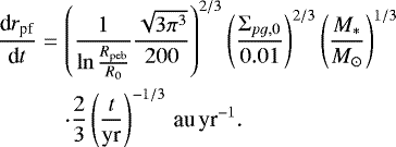
From these, we can define the timescale for the pebble formation front to reach the outer disc radius as follows:
 (20)
(20)
Thus, the pebble front location is in turn given by
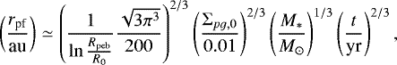 (21)
(21)
By putting these together, the pebble mass flux is written as follows:
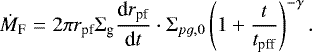 (23)
(23)
Finally, we calculated the pebble mass flux in our disc model. Since the pebble formation front is in the outer disc, we used the gas surface mass density in the irradiation region from Ida et al. (2016):
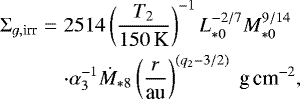 (24)
(24)
where T2 is a characteristic disc temperature in the irradiation region and T2 = 150 K in our default model, q2 = 3∕7 is the power in T ∝ r−q, the L*0 = L*∕L⊙ and M*0 = M*∕M⊙ are the stellar luminosity and mass scaled to the solar values, α3 = αacc∕10−3 is the disc accretion αacc scaled to a typical value, and 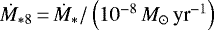 .
.
Substituting Eqs. (18), (20)–(22), and (23) into Eq. (23), we obtain the following:
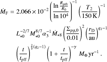 (25)
(25)
The evolution of this equation is shown in the right panel of Fig. 2.
In our simulations, we considered five different stellar metallicities: ![$\textrm{[Fe/H]}\,{=}\,\left(-0.5,\,-0.3,\,0.0,\,0.3,\,0.5\right).$](/articles/aa/full_html/2021/06/aa39210-20/aa39210-20-eq42.png) Thus, we covered a range of metallicities of planet-hosting stars that are related to the dust-to-gas surface mass densities Σdg = Σd∕Σg as follows:
Thus, we covered a range of metallicities of planet-hosting stars that are related to the dust-to-gas surface mass densities Σdg = Σd∕Σg as follows:
![\begin{equation*} \frac{\Sigma_{\textrm{dg}}}{\Sigma_{\textrm{dg},\odot}}\simeq10^{\textrm{[Fe/H]}}, \end{equation*}](/articles/aa/full_html/2021/06/aa39210-20/aa39210-20-eq43.png) (26)
(26)
where Σdg,⊙ = 0.01 is the value for the Solar System. Thus, in our model, the pebble mass flux is proportional to the square of the dust-to-gas surface mass density ratio. The dependence is not exactly the same, but similar to that of Lambrechts & Johansen (2014), where  .
.
The last column of Table 1 shows the total masses of pebbles accreting towards the star during the simulations for the solar metallicity case [Fe/H] = 0.0. The total masses vary over 19.4–597 ME for [Fe/H] = 0.0 in our disc models, and they vary by a factor of 3 above and below these values for the entire range of metallicities we considered: ~ 6.5–1791 ME. In comparison, Bitsch et al. (2019) obtained total pebble masses of 70–700 ME. Tychoniec et al. (2018) estimated that dust disc masses of Class 0 objects vary over 10–6000 ME, where a typical value is 248 ME and less than 10% of systems have masses above 1000 ME. Therefore, the range of total pebble masses we considered are consistent with observations.
Disc models 1–8.
2.2.3 Pebble accretion efficiency ϵ
The protoplanetary cores are exposed to the flux of pebbles, but they only accrete a fraction of the incoming flux. As stated before, we write the pebble accretion rate as Ṁcore = ϵṀF. Matsumura et al. (2017) adopted the accretion efficiency defined by Ida et al. (2016), which is valid in the settling regime:
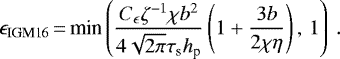 (27)
(27)
The 1 in parentheses ensures that the accretion efficiency does not become larger than unity. In this equation, ζ and χ are functions of the Stokes number τs and defined as

The pebble aspect ratio is defined as hp = Hp∕r, where Hp is the pebble scale height (Ida et al. 2016):
 (30)
(30)
Similarly, b = B∕r and B is an impact parameter for a pebble passing by the protoplanet with mass Mp :
![\[ B\simeq\min\left(\sqrt{\frac{3\tau_{\textrm{s}}^{1/3}R_{\textrm{H}}}{\chi\eta r}},\,1\right)\cdot2\kappa _{\textrm{OK12}}\tau_{\textrm{s}}^{1/3}R_{\textrm{H}}\,, \]](/articles/aa/full_html/2021/06/aa39210-20/aa39210-20-eq48.png)
where the left and the right terms in parentheses correspond to the Bondi and Hill regimes, respectively. The  is the Hill radius of the protoplanet,and the κOK12 is a reduction factor of the accretion proposed by Ormel & Kobayashi (2012) for τs ≫ 1 as:
![\[ \kappa _{\textrm{OK12}}\,{=}\,\exp\left(-\left(\frac{\tau_{\textrm{s}}}{\min\left(2,\,\tau_{\textrm{s}}^{*}\right)}\right)^{0.65}\right), \]](/articles/aa/full_html/2021/06/aa39210-20/aa39210-20-eq50.png)
with  . Also, Cϵ is defined as
 (31)
(31)
where the left and right terms represent 2D and 3D accretion, respectively. For the simulations, we scaled Cϵ by a factor Cϵ,i to take account of the orbital inclination effect. By assuming that the pebble volume density scales as  , the surface mass density between z ± B scales with:
 (32)
(32)
By normalising this factor with the value at z = 0, we obtain the following:
 (33)
(33)
More recently, Ormel & Liu (2018) studied the 3D pebble accretion efficiency by considering the effects of eccentricity, inclination, and disc turbulence:
 (34)
(34)
where A3 = 0.39 is a fitting constant to their pebble accretion simulations. The effective pebble aspect ratio is defined as
![\begin{equation*} h_{\textrm{p,eff}}\sim\sqrt{h_{\textrm{p}}^{2}+\frac{\pi\,i_{\textrm{p}}^{2}}{2}\left(1-\exp\left[-\frac{i_{\textrm{p}}}{2h_{\textrm{p}}}\right]\right)}, \end{equation*}](/articles/aa/full_html/2021/06/aa39210-20/aa39210-20-eq57.png) (35)
(35)
where ip is the inclination of a planetary orbit. The settling fraction is determined by integrating the accretion probability over the velocity distribution and is written as follows for turbulence operating only in the vertical direction:
![\begin{equation*} f_{\textrm{set}}\,{=}\,\exp\left[-a_{\textrm{set}}\left(\frac{\Delta v_{y}^{2}}{v_{*}^{2}}+\frac{\Delta v_{z}^{2}}{v_{*}^{2}+a_{\textrm{turb}}\sigma_{P,z}^{2}}\right)\right]\frac{v_{*}}{\sqrt{v_{*}^{2}+a_{\textrm{turb}}\sigma_{P,z}^{2}}}, \end{equation*}](/articles/aa/full_html/2021/06/aa39210-20/aa39210-20-eq58.png) (36)
(36)
where aset = 0.5 and aturb = 0.33 are other fit constants, Δvy and Δvz are azimuthal and vertical approach velocities, respectively, and σP,z is the vertical component of pebble root mean square velocity.
The left panel of Fig. 3 compares the accretion efficiencies for a ~ 0.1M⊕ planet from Ida et al. (2016; crosses) and from Ormel & Liu (2018; circles) as a function of τs. The estimated accretion efficiencies are similar for Ida et al. (2016) and Ormel & Liu (2018) over a wide range of τs, though the values from Ida et al. (2016) are generally slightly higher than those from Ormel & Liu (2018). In this work, we tested both types of the accretion efficiencies, and confirmed that the general trends are similar in both cases except that the mass growth is less efficient in the cases of Ormel & Liu (2018). In this paper, we focus on the simulations with the efficiency by Ida et al. (2016) ϵIGM16, but we discuss the effects of that by Ormel & Liu (2018) ϵOL18 briefly in Sect. 3.2.2.
2.2.4 Pebble isolation mass
The pebble isolation mass (PIM) is the protoplanetary mass at which the embryo becomes large enough to perturb the gas disc, modify the pressure gradient so that pebbles locally feel a tailwind rather than a headwind, and thus to halt the inward radial drift of pebbles (Morbidelli & Nesvorny 2012). This critical mass marks the end of the pebble accretion stage and thus is one of the key parameters to determine the outcome of planet formation. There are different formulations for the PIM in the literature, which we briefly discuss below.
Lambrechts et al. (2014) estimated the PIM as 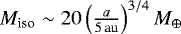 from hydrodynamic simulations, which we adopted for Matsumura et al. (2017). However, this study did not take account of the effects of the disc’s turbulent viscosity. More recently, Ataiee et al. (2018) and Bitsch et al. (2018) extended this study and investigated the dependence of the PIM on the disc aspect ratio, the pressure gradient of the disc as well as the viscosity. Ataiee et al. (2018) used 2D gas and dust hydrodynamic simulations, while Bitsch et al. (2018) used 3D gas-only hydrodynamic simulations with 2D integrations of particle trajectories. As discussed in Ataiee et al. (2018) and also shown in Fig. 3, the two studies have similar PIM trends, but details are different. Moreover, the differences become larger for the lower values of the viscosity αturb.
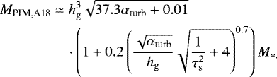
Bitsch et al. (2018) performed 3D hydro simulations over ![$\alpha_{\textrm{turb}}\,{=}\,\left[2\,{\times}\,10^{-4},\:6\,{\times}\,10^{-3}\right]$](/articles/aa/full_html/2021/06/aa39210-20/aa39210-20-eq60.png) to determine the PIM as follows:
to determine the PIM as follows:

A potential problem with this fit formula is that the saturation might not quite have been achieved for the lower end of αturb, as indicated in Fig. 3 of Johansen et al. (2019).
On the other hand, Ataiee et al. (2018) performed 2D hydro simulations over ![$\alpha_{\textrm{turb}}\,{=}\,\left[5\,{\times}\,10^{-4},\:1\,{\times}\,10^{-2}\right]$](/articles/aa/full_html/2021/06/aa39210-20/aa39210-20-eq62.png) and proposed the following PIM:
and proposed the following PIM:
 (39)
(39)
As seen in their Fig. 8, the expression agrees well with the 2D hydro simulations in the low-viscosity limit (αturb ~ 10−3), while the difference is about a factor of 3 for αturb ~ 10−2.
The right panel of Fig. 3 compares the pebble isolation mass model by Ataiee et al. (2018) with that of Bitsch et al. (2018). The figure also shows the transition mass from type I to type II migration as shown in the previous sub-section. Since the PIM measures the first appearance of the zero pressure gradient outside the planetary gap, the required depth is about 15% (Lambrechts et al. 2014) and is shallower than that for the migration transition of ~ 50% (Johansen et al. 2019). In other words, the planets are expected to first obtain the PIM and then reach the migration transition mass via gas accretion (or planetesimal accretion or core-core collisions). This implies that, unless the gas accretion is fast enough, the protoplanets are likely to migrate toward the central star on type I migration timescale (Johansen et al. 2019). However, since the PIM decreases towards the central star, it is likely for such type I migrators to eventually start gas accretion, and for migration to slow down as a result.
The PIM by Bitsch et al. (2018) is lower than the migration transition mass within ~ 10 au for αturb = 1 × 10⁻³ (see dashed green and dashed red lines, respectively), but it is higher for αturb = 1 × 10⁻⁴ (see solid green and solid red lines, respectively). The latter is counter-intuitive, since it indicates that a deeper gap is required for migration transition than for reaching the PIM. On the other hand, for the PIM model by Ataiee et al. (2018), the PIM is generally lower than the migration transition mass. Thus, for this work, we adopted the PIM by Ataiee et al. (2018)2.
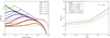 |
Fig. 3 Left: pebble accretion efficiency ϵ and the Stokes number for different values of the vertical turbulence strength αturb. The figure uses the planet-to-star mass ratio of 3 × 10⁻⁷ (i.e. ~ 0.1 ME for a Sun-like star), the gas disc aspect ratio of hg = 0.03, and the disc radial pressure gradient of η = 1.0 × 10⁻³ as in Fig. 4 of Ormel & Liu (2018). Circles show ϵ from Ormel & Liu (2018) and crosses show corresponding ϵ from Ida et al. (2016). Right: pebble isolation masses estimated by Ataiee et al. (2018; orange) and Bitsch et al. (2018; green), compared with our default case from Ida et al. (2016; blue). Also plotted are the critical migration transition masses (Eq. (10), red). |
2.2.5 Gas accretion onto a protoplanet
The rapid gas accretion onto a protoplanet starts when a protoplanetary core becomes massive enough so that the (quasi-) hydrostatic gas pressure can no longer support the envelope against the gravity. Following Ikoma et al. (2000), we assume this critical core mass for gas accretion is
![\begin{equation*} M_{\textrm{core,crit}}\simeq10\left[\left(\frac{\dot{M}_{\textrm{core}}}{10^{-6}{\mathrm{M_{E}/yr}}}\right)\left(\frac{\kappa}{1\,{\mathrm{cm^{2}/g}}}\right)\right]^{s}M_{E},\end{equation*}](/articles/aa/full_html/2021/06/aa39210-20/aa39210-20-eq64.png) (40)
(40)
where Ṁcore is the core accretion rate, s = 0.2 − 0.3, and κ is the grain opacity. For our simulations, we adopted s = 0.25 and κ = 1 cm2∕g, respectively. The equation assumes that the envelope is heated by the planetesimal accretion, and it is not immediately clear whether pebble accretion would provide a comparable heating. Recently, Ogihara & Hori (2020) explored this topic by using the 1D hydrostatic model with pebble accretion rates over 10−12 − 10−2 ME∕yr. They obtained the fitting function: 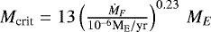 , which is consistent with the equation adopted here. We only became aware of their work while this manuscript was under revision, and thus we adopted Eq. (40) instead of theirs. The model implies that the gas accretion starts once the core accretion stops either because the PIM is reached or because the pebble flux runs out.
The gas accretion onto a protoplanet is limited both by how quickly a protoplanet can accrete gas and by how quickly a disc can supply gas to the protoplanet (e.g. Ida et al. 2018). The former condition is given by the Kelvin-Helmholtz (KH) timescale τKH as follows:
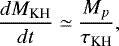 (41)
(41)
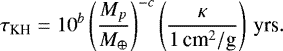
Parameters b and c are not well constrained. Ikoma et al. (2000) proposed  based on their numerical simulations, while Ida & Lin (2004) suggested that the parameters could take values up to
 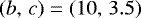 depending on different opacity tables, and they adopted
 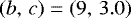 for their work. For this work, we adopted
  though we also tested other combinations. The KH timescale becomes shorter for smaller b and larger c, and shorter timescales lead to more massive final giant planet masses. However, beyond a certain point, the fast KH timescale does not help the growth any more because the gas accretion is limited by the efficiency of gas supply by the disc.
Regarding the latter condition, the disc nominally supplies gas at a rate Ṁ* (see Eq. (14)). For an actively accreting protoplanet, however, the reduced surface mass density effect as proposed by Tanigawa & Tanaka (2016) should be included, which we approximated as:

Putting these together, we adopted the following gas accretion rate as in Ida et al. (2018):
![\begin{equation*} \dot{M}_{\textrm{gas}}\simeq{\textrm{min}}\left[\dot{M}_{\textrm{KH}},\;\dot{M}_{*},\;\dot{M}_{\textrm{TT16}}\right].\end{equation*}](/articles/aa/full_html/2021/06/aa39210-20/aa39210-20-eq73.png) (45)
(45)
We should note that this reduction in the gas supply rate during the rapid gas accretion stage (i.e. ṀTT16) also further slows down type II migration (Tanigawa & Tanaka 2016; Tanaka et al. 2020). We did not take account of this effect in Eqs. (13) and (8) for simplicity, but we will investigate this issue further in future work.
2.3 Initial conditions
In this work, we considered eight different disc models around a Sun-like star as shown in Table 1, which lead to the stellar mass accretion rates and the corresponding pebble accretion rates as in Fig. 2. For each of these discs, we assumed five different stellar metallicities of [Fe/H] = −0.5, − 0.3, 0.0, 0.3, and 0.5. As stated earlier, we assume that the global angular momentum transfer is carried out mainly by the disc wind with αacc shown in the table, while the local disc-planet interactions are controlled by the disc’s turbulent viscosity constant αturb = 10−4 (see Sect. 3.2.1 for other values).
Figure 4 shows the outcome of in situ planet formation (i.e. no migration) in Disc 5 with the solar metallicity, starting with a protoplanetary core mass of 10−4M⊕. This initial mass is comparable to a Ceres mass, which is a characteristic mass for a planetesimal formed via streaming instability (Johansen et al. 2015; Simon et al. 2016). Differently from simulations presented in Sect. 3, the effect of the snowline is ignored here for simplicity. The top left panel compares the Kelvin–Helmholtz gas accretion timescale for the PIM core (orange) with the core formation timescale (i.e. the total time required for a core to reach the PIM, blue). The total in situ formation timescale of a gas giant planet will be comparable to the sum of these two timescales. For example, although the core accretion time is the shortest around 1 au, the PIM core there is too small to accrete gas efficiently. Thus, in our model, it is likely difficult to form a gas giant in situ at around 1 au, and the gas giant planet formation timescale becomes shortest around several au.
The right panel shows the total mass of a protoplanet reached after 100 Myr across the disc (orange), along with the total mass at different times of the growth calculations (blue curves). The solid green curve shows the PIM, while the dotted green curve shows the final core masses in the regions where the planetary masses never reach the PIMs. The figure indicates that protoplanets achieve the PIMs in most parts of the disc within a few au by ~ 105 yr and within ~10 au by ~ 106 yr. In this disc model, planetary growth is inefficient beyond ~10 au, because the accretion cross-section and thus the pebble accretion efficiency sharply decreases for a low-mass protoplanet in the outer disc. The corresponding pebble accretion efficiencies are shown in the bottom left panel. Although this figure is made based on the accretion efficiency by Ida et al. (2016), the trend is similar with the efficiency by Ormel & Liu (2018).
We compiled similar figures for other discs and found that gas giant planets do not form in situ in our disc models beyond ~ 20 au, if the initial core mass is comparable to that of Ceres. If typical planetesimals formed are about the size of Ceres (e.g. Johansen et al. 2015; Simon et al. 2016)throughout the disc, planetesimals have to grow via planetesimal-planetesimal collisions or via some other manner to reach ~ 10−2 M⊕ to form gas giants via pebble accretion beyond ~20 au. The trend shown here is largely consistent with Johansen & Lambrechts (2017), where growing a core from 10−5 M⊕ to 10−1 M⊕ via pebble accretion takes a few Myr at 30 au.
However, typical planetesimal sizes may be different depending on the disc environment. We can roughly estimate the planetesimal mass formed via streaming instability by considering the gravitational instability in the dust layer:
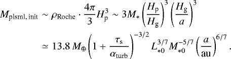 (46)
(46)
To get the final expression, we used the Roche density  , Eq. (30) for Hp∕Hg, and the disc aspect ratio of the irradiation region (Ida et al. 2016):
 (47)
(47)
With Eq. (46), the initial planetesimal mass becomes 10−4 M⊕ at ~ 2.8 au and increases to 10−2 M⊕ at ~83 au in Disc 5 (i.e. the same disc as in Fig. 4), which makes the giant planet formation possible out to ~ 40 au. For longer-lived, more massive, or more metal-rich discs, giant planets can form out to or beyond 100 au. In this paper, we choose conservative initial conditions and do not place the planetary cores beyond 20 au.
Exercises similar to that of Fig. 4 also suggest that the maximum giant planet mass achievable in our simulations is a few to several thousand M⊕. The upper mass limit is determined partly by the planet’s efficiency of gas accretion and partly by the disc’s capability of providing gas (see Sect. 2.2.5). It may be possible to achieve ~ 104 M⊕ with an extreme choice of parameters such as (b, c) = (7, 3) in a highly turbulent disc with αturb = 10−2 or in a massive, long-lived disc (e.g. 0.2 M⊙ with tdiff ~ 10 Myr). However, the former tends to lose planetary cores to the star due to efficient migration, while the latter-type of discs may be relatively rare. Taking a more extreme set of parameters would not help the further mass growth because the gas accretion is limited by the disc’s gas supply as seen in Eq. (45). By assuming the initial masses of protoplanets with Eq. (46), the maximum mass becomes ~ 50 MJ ~ 1.6 × 10⁴ M⊕ for massive, metal-rich, long-lived discs. We discuss this issue further in Sect. 4.3.
We ran 240 multiple-planet-core simulations as well as about a hundred more single-planet core simulations. In all of these runs, we assumed a Sun-like star. For the main simulations, we have ten cores per system with the initial mass of 10−2 M⊕~ 100 MCeres over 0.5–15 au3. The inner edge of the disc is set at 0.1 au for all of our simulations. This is rather arbitrary, but is adopted partly because the timesteps required to resolve an orbit become too small within this radius to run a simulation for 100 Myr, and partly because tidal interactions with the star also become important there, and we do not explicitly include this effect in our code (however, see Sect. 3.1.2). Each core has a randomly assigned initial eccentricity of ![$e\,{=}\,\left[0,\,0.01\right]$](/articles/aa/full_html/2021/06/aa39210-20/aa39210-20-eq77.png) , the corresponding inclination of i (rad) = 0.5e, and randomly chosen phase angles. Planets are also considered ‘removed’ beyond 1000 au in our simulations. In summary, we simulated the growth and orbital evolution of the ten cores in the eight different disc models shown in Table 1 with five different stellar metallicities. Six simulations are run for each combination of parameters, which makes the total number of main simulations 240.
, the corresponding inclination of i (rad) = 0.5e, and randomly chosen phase angles. Planets are also considered ‘removed’ beyond 1000 au in our simulations. In summary, we simulated the growth and orbital evolution of the ten cores in the eight different disc models shown in Table 1 with five different stellar metallicities. Six simulations are run for each combination of parameters, which makes the total number of main simulations 240.
Besides the effects of disc models and stellar metallicities, we have also explored the effects of the Kelvin-Helmholtz timescales, the turbulent viscosity αturb, and the pebble accretion efficiency. We discuss some of these in Sect. 3.2.1 for single-planet simulations. For main simulations, these parameters are set as (b, c) = (8, 3), αturb = 10−4, and ϵ = ϵIGM16, respectively.
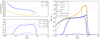 |
Fig. 4 Top left panel compares the total time to form the protoplanetary core with the pebble isolation mass (orange, τpeb) with the Kelvin-Helmholtz gas accretion timescale for the PIM core (blue, τKH). The right panel shows the planetary mass growth at different times starting from 10−4 ME in Disc 5. The solid green line shows the PIM, while the dotted green line represents the core masses at 100 Myr (i.e. at the end of the simulations) for the cores not reaching PIMs. The orange line shows the final total mass. Here, the effects of the snow line are ignored. The bottom left panel shows the corresponding pebble accretion efficiencies by Ida et al. (2016) at different times as a core grows from 10−4 ME. |
3 Results
In Sect. 3.1, we compare the results of main numerical simulations of multiple-planet cores with observed systems, by focusing on the effects of disc parameters such as mass, dissipation timescale, and metallicity. In Sect. 3.2.1, we discuss the effects of the turbulent viscosity alpha αturb as well as the pebble accretion efficiency ϵ through single-planet simulations. Throughout this paper, we use the radial-velocity detected, confirmed extrasolar planets obtained from the NASA Exoplanet Archive4 as ‘observed planets’. We do not include transit planets for comparison with simulations unless we state otherwise, because the transit surveys have a large bias towards close-in planets due to the detectability dependence of ∝ a−1.
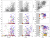 |
Fig. 5 Comparison of distributions of parameters for the observed exoplanets and left, middle, and right panels are Mp − e, a − e, and a −Mp distributions, respectively. The top panels show observed data from the RV-detected planets. The bottom panels show all the simulated planets at the end of the simulations (100 Myr), while the middle panels show observable planets with the RV detection limit of 1 m s−1 and a ≤ 10 au. The black dashed line shown on a − Mp panels corresponds to 1 m s−1 limit. The shaded areas in a − e and a −Mp distributionsindicate that the inner disc edge of our model is at 0.1 au, and thus we do not intend to reproduce planet distributions there. Circles and crosses represent giant (≳ 0.1 MJ) and low-mass (<0.1 MJ) planets, respectively, and the red, orange, green, blue, and purple colours correspond to stellar metallicities of − 0.5, −0.3, 0.0, 0.3, and 0.5, respectively. Some planets are clustered around 0.1 au because the disc’s inner edge is set there. |
3.1 The effects of disc mass, dissipation timescale, and stellar metallicity
First, we present the overall results of simulations in Sect. 3.1.1 and show that the overall trends of distributions of giant planets are well-reproduced. Then we will focus on formation of different types of giant planets in Sects. 3.1.2 and 3.1.3.
3.1.1 Overall results of multiple protoplanetary-core simulations
In this paper, we define planetary bodies as having a mass ≥ 0.1 M⊕, because this is about the Mars mass and also roughly the smallest mass of observed exoplanets. We also divided planets into two groups for simplicity: giant planets (≥0.1 MJ ~ 30 ME) and low-mass planets (<0.1 MJ). This division is rather arbitrary, but it is motivated by a mass above which the semi-major axis mass distribution of observed exoplanets appears to change.
Figure 5 shows the overall results of our simulations compared to the observed planetary systems. The left, middle, and right panels correspond to Mp − e, a − e, and a − Mp distributions, respectively, for all the simulated planets (bottom panels), observable simulated planets (middle panels), and observed planets (top panels). For the ‘observable’ planets, we applied the RV detection limit of 1 m s−1 and a ≤ 10 au. As seen in the figure, the simulated planets reproduce the overall trends of Mp − e, a − e, and a − Mp distributions of extrasolar giant planets well. We note that the disc inner edge of our simulations is set at 0.1 au and the code does not include the tidal evolution effects. Therefore, the cluster of simulated planets near 0.1 au and their slightly elevated eccentricities compared to observed systems are not surprising.
As seen in the a − Mp distribution, our simulations successfully generate all kinds of giant planets including hot Jupiters (HJs, a ≲ 0.1 au), warm Jupiters (WJs, 0.1 au ≲ a ≲ 1 au), cold Jupiters (CJs, 1 au ≲ a ≲ 20 au), and super-cold Jupiters (SCJs, a ≳ 20 au). As already shown by Ida et al. (2018), CJs are formed successfully since the new type II migration is slower than the classical one and since the low disc turbulence αturb = 10−4 is assumed in the two-α disc model We discuss the formation of HJs and SCJs further in Sects. 3.1.2 and 11, respectively.
As in Matsumura et al. (2017), we still have trouble reproducing the orbital properties of low-mass planets within ~ 1 au, because many protoplanetary cores are lost to the star since type I migration is too efficient and the disc edge is not sharp enough to retain them efficiently. This may not be too surprising because, although we have improved our code significantly, as seen in Sect. 2, none of those mechanisms help to slow type I migration. Lambrechts et al. (2019) and Izidoro et al. (2021) successfully produced rocky super-Earth systems over 0.1–1 au, where we lost many such planets due to rapid migration. This is partly because their disc ages are much shorter than ours and partly because their planets are trapped in mean motion resonances more efficiently at the disc edge since they terminate planet migration there. In our simulations, some gas discs’ lifetimes are as short as a few Myr like their simulations, but others are 10 Myr or longer. The long lifetimes are motivated by recent observations as stated before, but it also leads to the loss of the majority of low-mass planets as expected.
Having this bias of low-mass planets in mind, our simulations suggest that there may be a group of eccentric low-mass planets in the outer disc (≳10 au). In our simulations, they are coming from Discs 2 and 3, which are not too massive (0.06 M⊙ and 0.02 M⊙) and have a short dissipation timescale of 0.1 Myr. As discussed further in the next sub-section, these are protoplanetary cores which did not have enough time to become giant planets. Since we reproduce the overall trends of distributions of giant planets well while those of low-mass planets are poorer due to the uncertainties in type I migration, we focus on the outcomes of giant planets for the rest of this paper.
Although we compare our simulations with observed giant planets, it is not our intention to exactly reproduce the distributions of orbital and physical parameters of extrasolar planets. Such a comparison does not make sense for this study since it would force us to make assumptions, for example, that disc models 1–8 exist with an equal probability and that the inner and outer disc radii are the same for all the discs, which are unlikely to be true in reality. Having said that, Fig. 6 presents the comparison of distributions of the semi-major axis, planetary mass, and eccentricity for observed (dashed lines) and simulated (solid lines) giant planets. The left panels include all the giant planets (≥ 30 ME) beyond 0.1 au, while the right panels include only those with masses 30–3000 ME and semi-major axes 0.1–10 au. Only the planets beyond 0.1 au are chosen because our inner disc edge sits there, and because we do not include tidal evolution in our simulations directly (however, see Sect. 4.2).
By eye, the agreement between observed and simulated distributions are good for both planetary masses and eccentricities. In fact, for the massdistribution in the left panel, the Kolmogorov–Smirnov (K–S) test could not reject the null hypothesis with the statistics of 0.092 and the P value of 0.11. The agreement is poor for semi-major axis distributions, which indicates that we overproduced CJs compared to WJs. This may imply that we need to understand type I migration better to produce cores of these giants and/or that the low disc turbulence αturb is not appropriate for all the systems. Nevertheless, the overall good agreement with observed properties is encouraging.
As seen in Mp − e and a − e distributions of Fig. 5, as well as the middle panels of Fig. 6, our simulations also reproduce the wide range of eccentricities observed for giant planets. Compared to the lack of highly eccentric giant planets seen in Matsumura et al. (2017) and Bitsch et al. (2019), this is a great improvement. We suspect that the success is partly due to a range of disc parameters leading to a larger number of giant planets per system than Matsumura et al. (2017), and partly due to low efficiencies of eccentricity and inclination damping (see Sect. 4.7).
In Matsumura et al. (2017), the average number of giant planets formed per system throughout the simulations was typically about two for no-migration cases. In our new simulations, on the other hand, the average number of giant planets can be much higher, as seen in Fig. 7. The number of giant planets decreases over time due to dynamical instabilities, which lead to the population of giant planets with high eccentricities. Overall, the number of giant planets tends to be higher when a disc has higher mass, higher metallicity, and longer dissipation timescale. For Disc 3, which has the lowest mass and the shortest dissipation timescale, giant planet formation is a rare event, and it happens only for the highest metallicity case. The average number of giant planets formed in high-mass and/or high-metallicity discs is typically a few or more and decreases over time to ~ 2 in the end. However, we note that the number of giant planets per system was also very high in Bitsch et al. (2019; typically about 5), and we discuss this issue further in Sect. 4.7.
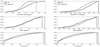 |
Fig. 6 Distributions of semi-major axis (top), planetary mass (middle), and eccentricity (bottom). The solid and dashed lines correspond to simulated and RV-detected planets, respectively. The left panels include all the giant planets beyond 0.1 au, while the right ones are limited to orbital radii of 0.1–10 au and masses up to 3000 ME. The K–S test cannot reject the null hypothesis for the mass distribution on the left with the statistics of 0.092 and the P value of 0.11, but rejects the null hypothesis for all other cases. Our simulations clearly produce more giant planets in the outer region compared to observed systems. However, the agreements are not bad by eye for both masses and eccentricities. |
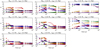 |
Fig. 7 Evolution of the average number of giant planets (solid) and low-mass planets (dotted) for different disc models. Red, orange, green, blue, and purple correspond to stellar metallicities of -0.5, − 0.3, 0.0, 0.3, and 0.5, respectively. |
3.1.2 Formation of hot Jupiters
There are three main pathways to form hot HJs: in situ formation (e.g. Batygin et al. 2016), disc migration after the formation of a giant planet beyond the snow line (e.g. Lin et al. 1996), and the tidal circularisation of a highly eccentric orbit of a giant planet(e.g. Fabrycky & Tremaine 2007; Nagasawa et al. 2008; Naoz et al. 2011; Wu & Lithwick 2011). Here, the insitu formation includes both the cases where protoplanetary cores also form in situ (e.g. Chiang & Laughlin 2013; Boley et al. 2016) and the cases where cores form further out, migrate to the inner disc, and then accrete gas there (e.g. Coleman & Nelson 2016b; Matsumura et al. 2017). In this section, we evaluate these pathways by using our simulations and argue that differences in stellar metallicities may naturally lead to different pathways.
Figure 8 shows two-panel plots of eight different disc models, where each disc is run with five different stellar metallicities. For each disc model, the bottom panel shows a histogram of giant planet formation timescales, while the top panel shows how far from the initial orbital radii giant planets are formed. As discussed in the previous section, we assume that a protoplanet becomes a giant planet once its mass surpasses 0.1 MJ.
As seenin bottom panels of different disc models, almost all discs form giant planets regularly except for Disc 3. For the disc models we considered, the median formation timescales are short (~ 0.1–1 Myr) compared to an often-quoted typical disc lifetime of ~ 3 Myr. This confirms that pebble accretion is an efficient way of forming giant planets within a disc’s lifetime.
The top panels of different disc models in Fig. 8 compare the ratio of the ‘formation’ semi-major axis to the initial semi-major axis: aform∕ain with the formation timescales. Here, again, the formation semi-major axis is where a planetary mass reaches 0.1 MJ. The red, orange, green, blue, and purple symbols correspond to different metallicities of [Fe/H] = −0.5, − 0.3, 0.0, 0.3, and 0.5,respectively. As expected, giant planets form more quickly in higher metallicity environments within the same disc model.
In discs with short dissipation timescales (Discs 1–3, tdiff = 0.1 Myr), we find that giant planets often form near their initial locations. On the other hand, in discs with longer dissipation timescales (Discs 4 to 9, tdiff = 1–10 Myr), there are two types of giant planets: some are forming near their initial locations (often cores beyond several au), and others are forming after some migration. In the case of the latter, the formation radii tend to be about 1 to 2 orders of magnitude smaller than the initial orbital radii. In Discs 4–9, when metallicities are low [Fe/H] ≲−0.3, cores tend to migrate and then accrete gas to become either WJs or HJs. On the other hand, when metallicities are high [Fe/H] ≳ 0.0, outer cores tend to become CJs, while inner cores migrate to form WJs and/or HJs. However, in these cases, the inner cores are often removed via planet-planet interactions as the gas disc dissipates, and the final systems include either only CJs or HJs along with CJs. Thus, in our simulations, when HJs form in situ after their cores migrated to the inner disc, they tend to be in a low-metallicity disc, though they can also be formed in a higher metallicity disc.
Figure 9 shows the semi-major axis mass distribution of giant planets for each disc model. Combined with the results of Fig. 8, this figure shows two types of outcomes of giant planet formation. In rapidly dissipating or low-mass discs (Discs 1, 2, 3, and 6), low-mass (typically less than a few Jupiter masses) and cold (orbiting beyond ~ 1 au) giant planets are often produced. In these discs, lower metallicities lead to lower mass giant planets as expected, and the range of masses across different metallicities is about an order of magnitude. In more slowly dissipating, moderate-to-high-mass discs (Discs 4, 5, 7, and 8), on the other hand, giant planets have a much wider distribution of orbital radii (two to three orders of magnitude),as expected from Fig. 8. Planetary masses per disc model are largely comparable to one another and weakly depend on metallicities (see Sect. 4.6), but cores migrated further tend to have lower masses.
This a − Mp relation of mass increasing with orbital radius is likely to arise from the reduced gas accretion rate onto the gap-opening core ṀTT16 in Eq. (45). Assuming that the gas accretion timescale can be written as  , the planetary mass has the dependence of:
  . Since the disc aspect ratios in viscous and irradiation regions in our disc model have
  and
and  , respectively (see Ida et al. 2016), the expected mass dependences on semi-major axes are
  and
and  , respectively.For Discs 4, 5, 7, and 8 in Fig. 9, these trends are shown in dashed and dotted lines, respectively, and the agreement is very good for these cases.
Our simulations do not explicitly include tidal interaction effects between the central star and planets, so we cannot directly measure the production rate of a HJ via tidal circularisation. However, we selected planets that could have experienced significant tidal evolution and applied the weak-friction tidal interaction model (e.g. Hut 1981). For giant planets that have a pericentre radius of  au and a semi-major axis a ≥ 0.2 au (i.e. an eccentricity of e ≥ 0.5) at any time during the simulation, tidal evolution is calculated. The results are plotted in Fig. 10. As in Matsumura et al. (2010), we scaled a modified tidal quality factor of
 (48)
(48)
where Q′≡ 1.5Q∕k2 is a modified tidal quality factor, Q is a tidal quality factor, k2 is the Love number of degree 2, n is the mean motion, and the subscript 0 represents their initial values. In our calculations, we assumed the initial stellar and planetary modified tidal quality factors to be  and
and  , respectively. Since a typical age of a planet hosting star ranges from 1–10 Gyr, we have run the tidal evolution simulations for 3 Gyr.
The left panel of Fig. 10 shows the semi-major axis eccentricity distribution of these planets before (open circle) and after (filled circle) tidal evolution, where different colours correspond to different stellar metallicities. As expected from the higher planet formation efficiency seen in high metallicity environments (see Fig. 7, for example), most planets that achieved high enough eccentricities in the first place are in the high-metallicity discs with [Fe/H] ≳ 0.0.
Since we do not know what kinds of discs or disc evolution paths dominate in reality, the fraction of HJ systems with respect to all the simulations cannot be compared with the observed fraction of HJ systems. However, we can attempt to estimate the fractions of giant-planet systems with HJs. About 10% of Sun-like stars are known to have giant planets, while roughly 0.5–1% of such stars have HJs (Winn 2018). This implies that, roughly speaking, ~ 5–10% of giant-planet hosting stars have at least one HJ. In our simulations, out of 240 runs, 175 formed at least one giant planet at some point during 100 Myr simulations. Out of these 175 systems, 10 formed HJs that have semi-major axes less than 0.1 au after 3 Gyr. Thus, 10∕175 ~ 5.71% of a giant-planet-forming system led to the formation of at least one HJ. If we relax this condition to the final semi-major axis within 0.2 au, the frequency becomes 38∕175 ~ 21.7%. These are reasonable values compared to the observed fraction of HJ systems among systems with giant planets: ~ 5–10%. We note that the occurrence rate depends on the choice of the initial distribution of disc parameters, and thus the high occurrence rate suggested by the simulations does not necessarily mean that our models overestimate the occurrence rate.
The right panel of Fig. 10 shows the corresponding eccentricity-inclination distribution of these planets before (open circles) and after (filled circles) applying tidal evolution. We note that the colours here indicate the final semi-major axes rather than the stellar metallicities. The overall trend is similar to what Nagasawa & Ida (2011) pointed out for observed exoplanets –planets with low eccentricities have a wide range of inclinations, while those with moderate eccentricities have low inclinations.Our simulations indicate that this trend breaks down at larger orbital radii, because the orbits of some planets cannot be circularised quickly enough.
From the figure, it is also clear that high-inclination planets initially had high eccentricities as well. This outcome of tidal evolution reflects the fact that the orbital circularisation is largely controlled by tidal dissipation inside the planet, while the spin alignment iscontrolled by tidal dissipation inside the star (i.e. the stellar spin aligns with the orbit normal rather than the other way around). Since the former takes place faster than the latter, the orbital eccentricity becomes small, while the orbital inclination does not change dramatically.
These outcomes lead to an expectation about the effects of stellar metallicities on HJ formation pathways — around low-metallicity stars, HJs tend to form via the migration of cores followed by in situ gas accretion, while around high-metallicity stars, they can form either via migration or via the tidal circularisation of eccentric orbits. One way to distinguish these two cases is to check the relation between the orbital inclination and the stellar metallicity. The HJs formed in situ or via migration are more likely to have low inclinations, while the tidally circularised planets are expected to have a wide range of inclinations. We discuss this matter further in Sect. 4.2.
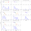 |
Fig. 8 Top: ratio of the semi-major axis of a giant planet when it became giant (i.e. mass reaches 0.1 MJ) with respect to the initial semi-major axis for different disc models. The red, orange, green, blue, and purple symbols correspond to stellar metallicities of −0.5, −0.3, 0.0, 0.3, and 0.5, respectively. Bottom: formation timescales of giant planets. The vertical dashed line indicates the median value. |
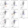 |
Fig. 9 Semi-major axis mass distribution of giant planets at the end of all the simulations for different disc models. The red, orange, green, blue, and purple colours correspond to stellar metallicities of −0.5, −0.3, 0.0, 0.3, and 0.5, respectively. The dashed and dotted lines in Discs 4, 5, 7, and 8 are expected mass trends in viscous and irradiation regions, respectively (see text). |
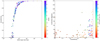 |
Fig. 10 Left: semi-major axis eccentricity distribution of planets before (open circle) and after (filled circle) tidal evolution. Different colours correspond to the stellar metallicity. Highly eccentric planets tend to belong to higher metallicity discs. Right: the corresponding eccentricity-inclination distribution. However, the colour does not represent the metallicity, but the final semi-major axis. Closer in planets tend to have either a low eccentricity and a range of inclinations, or a moderate eccentricity with a low inclination. |
3.1.3 Formation of super-cold Jupiters
The observations show that some giant planets have very wide orbital radii, ranging from a few tens of au to a few thousand au. In the pebble accretion model, we expect either (1) an SCJ forms in situ, or (2) a gas giant forms within ~ 20 au and then gets scattered into the outer disc. Again, the in situ formation here includes both the case where an SCJ directly forms in the outer disc, and the case where a protoplanetary core scattered into the outer disc accretes gas to become a giant planet there (Kikuchi et al. 2014). Since we did not place cores beyond 20 au, SCJs did not form directly in the outer disc in our simulations.
As seen in Fig. 8, most giant planets in our simulations ‘form’ (i.e. mass exceeds 0.1 MJ in our definition) near or inside the initial orbital radii. Therefore, most SCJs in our simulations are generated via scenario (2) (i.e. formed and then scattered), and not via scenario (1). We note, however, that our simulations preclude the scenario of Kikuchi et al. (2014). The key to forming SCJs in Kikuchi et al. (2014) was that the orbits of scattered cores get circularised efficiently via the accretion of high angular momentum gas in the outer disc. Since our disc only stretches out to 100 au, even when there was a scattered core, the core would repeatedly encounter the larger planet that scattered the core in the first place, and an SCJ does not form efficiently.
When an SCJ is formed via scenario (2), our simulations indicate the following. First, a stellar metallicity tends to be high ![$\left[\textrm{Fe/H}\right]\gtrsim0.0$](/articles/aa/full_html/2021/06/aa39210-20/aa39210-20-eq88.png) in a system with a SCJ. As seen in the left panel of Fig. 11, all but one giant planet beyond 20 au are from such systems. One giant planet is at around 30 au in the system with
in a system with a SCJ. As seen in the left panel of Fig. 11, all but one giant planet beyond 20 au are from such systems. One giant planet is at around 30 au in the system with ![$\left[\textrm{Fe/H}\right]\,{=}\,{-}0.5$](/articles/aa/full_html/2021/06/aa39210-20/aa39210-20-eq89.png) , but its mass is relatively low and ~40 M⊕. This trend is not surprising, because higher metallicity discs tend to form multiple giant planets without much migration (see Fig. 8) and thus are prone to dynamical instabilities that can scatter giant planets outward.
, but its mass is relatively low and ~40 M⊕. This trend is not surprising, because higher metallicity discs tend to form multiple giant planets without much migration (see Fig. 8) and thus are prone to dynamical instabilities that can scatter giant planets outward.
Second, the orbit of an SCJ tends to be eccentric and out to a few hundred au. It is difficult to scatter a giant planet beyond that and retain it when it is formed within ~ 20 au. The tendency towards a non-zero eccentricity is a direct outcome of the scattering event and thus is not surprising. In our simulations, the eccentricity of SCJs ranges over e ~ 0.2–0.9 with the mean value of 0.56.
Third, an SCJ tends to be accompanied by another giant planet. Our simulations show ~ 78.6% of SCJs (22/28) are in two- or three-giant-planet systems, while ~21.4% (6/28) are in single-planet systems. The right panel of Fig. 11 shows the semi-major axis ratio of a companion planet to the furthermost SCJ as well as their mass ratio. In multiple-planet systems, the furthermost SCJ tends to have a less massive companion interior to its orbit (15∕22 ~ 68.2%) rather than a more massive one (7∕22 ~ 31.8%). Thus, the scattering event tends to place a more massive planet outward and a lower-mass companion inward in our simulations.
The preference for the inner, lower-mass companion is opposite to what has been observed in previous studies (e.g. Marzari & Weidenschilling 2002; Nagasawa et al. 2008; Ida et al. 2013), where a more massive planet was scattered inward with a higher probability of > 80%. However, all of these studies started with the configuration where the inner planet is the most massive one (2 MJ, MJ, MJ). Since the higher mass planets tend to stay closer to the initial location upon scattering (Chatterjee et al. 2008), it may not be surprising that the more massive planet stayed in the innermost orbit in these studies. In our simulations, on the other hand, more massive planets tend to form in the outer part of the disc (see Fig. 4, for example). Therefore, it is not surprising that there is a preference towards the outermost planets being more massive than the inner ones because of their inertia and the difficulty of switching orbits. We discuss their formation and distributions further in Sect. 4.4.
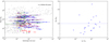 |
Fig. 11 Left: semi-major axis mass distribution of giant planets at 100 Myr. The error bars represent the locations of pericentre and apocentre and thus show how eccentric orbits are. Asbefore, red, orange, green, blue, and purple correspond to stellar metallicities of −0.5, −0.3, 0.0, 0.3, and 0.5, respectively. The circles, squares, and crosses correspond to single-planet, multiple-giant-planet, and multiple-planet but single giant planet systems, respectively. Right: mass and semi-major axis ratios for the furthermost SCJ and its companion. |
3.2 The effects of other parameters
In this sub-section, we show the effects of the turbulent viscosity αturb as well as the pebble accretion efficiencies.
3.2.1 The effects of the turbulent viscosity alpha parameter αturb
For the bulk simulations, we assumed αturb = 10−4. In this sub-section, we investigate the dependence of pebble accretion simulations on the turbulent alpha parameter by using single-planet-core simulations and by comparing αturb = 10−3 and 10−5 cases to the default ones with αturb = 10−4. We did not use all the disc models but focused on representative cases of Discs 2, 5, and 8, for which the initial disc mass is the same, 0.06 M⊙, and the diffusiontimescales are 0.1, 1.0, and 10 Myr, respectively. The initial semi-major axes of protoplanets are chosen to be ~ 3, 5, 7, and 10 au, which are all beyond the snowline initially. This is a rather narrow range compared to ~ 0.5 − 15 au in the bulk simulations, but they are chosen so that we can test the likelihood of forming giant planets. The stellar metallicity for all the simulations in this sub-section is the solar value of [Fe/H] = 0.0. Other parameters used for the default case are (b, c) = (8, 3) for the Kelvin–Helmholtz timescale, and the pebble accretion efficiency of ϵIGM16.
Figure 12 shows the outcomes of single-core simulations with αturb = 10−3, 10−4, and 10−5. From the cases with αturb = 10−4, we can confirm the trends described in previous sections: Disc 2 forms rather low-mass CJs, while Discs 5 and 8 form fully grown giant planets across a range of orbital radii.
For the cases of αturb = 10−3, most planets migrate to the edge of the disc (0.1 au here), except for Disc 2, where relatively low-mass giant planets form over a range of orbits. The loss of the majority of protoplanetary cores to the disc’s inner edge is similar to Matsumura et al. (2017), where we have also adopted αturb = 10−3. However, differently from Matsumura et al. (2017), the formation of relatively low-mass CJs is possible here largely due to the new migration prescription we adopted (see Sect. 2.1). The results are consistent with what we would expect from those in Sect. 3.1. For the higher viscosity αturb, the PIM is higher, and thus planet formation becomes too slow (compared to type I migration) to form giant planets in Discs 5 and 8. The giant planets are formed only in the most rapidly dissipating disc (Disc 2), which provides a high mass flux for a short period of time, but their masses are low for giant planets.
For the cases of αturb = 10−5, the formation rate of giant planets, especially CJs beyond 1 au, is even higher than the default case of αturb = 10−4 for Discs 5 and 8, while only super-Earths are formed for Disc 2. The trends are again consistent with those seen in Sect. 3.1. For the lower αturb, both the PIM and the migration transition mass are lower. Therefore, protoplanetary cores start gas accretion at lower mass and also tend to switch from type I to type II migration earlier and survive. In Disc 2, the cores are too small to become giant planets within the disc’s lifetime, while in Discs 5 and 8, CJs can be formed over a wide range of orbital radii.
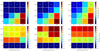 |
Fig. 12 Outcome of single-planet formation simulations with the default setting (i.e. (b, c) = (8, 3) for the Kelvin–Helmholtz timescale, [Fe/H] = 0.0, and the pebble accretion efficiency by IGM16) with αturb = 10−3 (left panels),10−4 (middle panels), and 10−5 (right panels). The top panels show the final semi-major axis of a single planet for different initial semi-major axes and disc models. The bottom cells marked as ‘Init’ correspond to the initial semi-major axes that are common for all disc models. The bottom panels present the final planetary masses in log scale. The bottom cells represent the initial protoplanetary masses of 0.01M⊕ for all the cases. |
3.2.2 The effects of the pebble accretion efficiency
Figure 13 shows the same as Fig. 12, but with the pebble accretion efficiency by Ormel & Liu (2018) ϵOL18 (see Eq. (34)) instead of that by Ida et al. (2016) ϵIGM16 (see Eq. (27)). Despite the small differences between the two accretion efficiencies seen in Fig. 3, these two figures look dramatically different. There are a couple of reasons here. First, a factor of a few difference in accretion efficiencies actually leads to a large difference. For example, a factor of three difference corresponds to the metallicity difference between [Fe/H] = 0.0 and [Fe/H] = 0.5. Second, the accretion efficiency by Ormel & Liu (2018) is more sensitive to the inclination. For example, among cases shown in Fig. 13, a protoplanet at ~5 au consistently produces a much lower mass planet compared to the neighbouring ones. This is because the randomly chosen initial inclination for this core is i ~ 0.26 degree (i.e. e ~ 0.01) as opposed to i ≲ 0.14 degrees (i.e. e ≲ 0.005) for the others. Compared to the circular, coplanar case, the accretion efficiency ϵOL18 decreases by more than an order of magnitude with e ~ 0.01 and i ~ 0.26 degree, while the difference is about a factor of a few with e ≲ 0.005 and i ≲ 0.14 degrees.
Besides the slow growth of a protoplanet at ~5 au, the outcomes shown in Fig. 13 are consistent with Fig. 12 and the expectations from Sect. 3.1. With αturb = 10−5, giant planets are formed across a range of disc radii for Discs 5 and 8. Compared to the corresponding cases in Fig. 12, although the final masses of giant planets are comparable, the final semi-major axes are smaller in these cases. This is because it takes longer to form planets with lower efficiencies, and planetary cores migrate more before becoming giant planets in these cases. In Disc 2, only very low-mass planets are formed, which is also consistent with this expectation.
With αturb = 10−4, none of the cases with the solar metallicity lead to giant planet formation. With αturb = 10−3, trends are similar to the cases in αturb = 10−4, but HJs are formed at the disc’s inner edges in Disc 5. Since no giant planets are formed in the corresponding cases in Fig. 12, these cases may appear surprising. What happened here is that protoplanets grew slower with the lower pebble accretion efficiencies, stayed longer beyond the snow line, and obtained slightly more massive cores before migrating into the inner disc region, where they become HJs by accreting gas.
For completion, we also ran a set of multiple-core simulations with ϵOL18 and showed the results in Fig. 14. Here, we only use Discs 2, 5, and 8, but the other parameters are the same as those shown in Sect. 3.1 with the default accretion efficiency ϵIGM16. The overall distributions are similar to Fig. 5 for all the parameters, except that giant planets are mostly formed with high metallicities [Fe/H] ≳ 0.3. This is consistent with the expectation from single-core simulations shown above. The lack of very massive giant planets (≳ 2000 ME) compared to Fig. 5 is unlikely to be the real feature. As seen in Fig. 9, most massive giant planets are formed in most massive discs (0.2 M⊙ in our case), while all the discs used inthis figure have 0.06 M⊙. Therefore, to have distributions similar to Fig. 5 with the pebble accretion efficiency ϵOL18 by Ormel & Liu (2018), we would probably need to assume lower turbulence alpha αturb < 10−4 and very low inclinations for initial protoplanetary cores.
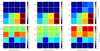 |
Fig. 13 Same as Fig. 12, but with the pebble accretion efficiency of Ormel & Liu (2018) rather than that of Ida et al. (2016). |
4 Discussion
In this section, we further discuss our results by focusing on several key topics. First, we compare planet occurrence rates obtained from our simulations with observations in Sect. 4.1. Then, we discuss formation of HJs (Sect. 4.2) and SCJs (Sect. 4.4). We also discuss to what orbital radii planets can be formed via pebble accretion and how massive planets can become in Sect. 4.3, and discuss metal and gas mass fractions of planets in Sect. 4.5. Finally, we compare our results with planetesimal accretion work (Sect. 4.6) as well as other pebble accretion work (Sect. 4.7).
4.1 Planet occurrence rates
The top panel of Fig. 15 shows the overall distribution of orbital periods of giant planets from our work. The blue and orange histograms correspond to the distributions of simulated planets and tidally evolved planets from Sect. 3.1.2, respectively. The strong peak seen around 10 days comes from the inner disc edge being set at 0.1 au in our simulations, and the actual distribution around this period should be broader depending on the locations of the inner disc edges. Otherwise, the overall distribution shows that CJs near 103 –104 days are most abundant, and the number decreases for planets interior and exterior to these orbits.
The bottom panel of Fig. 15 shows the corresponding occurrence rates compared with observed slopes. Following the approach by Winn (2018), we write the occurrence rate as:  , where n = Npl∕N* is the ratio of the number of giant planets to that of the host star, while Δ log P = 0.23 is chosen so that the comparison with Fig. 3 of Winn (2018) is easier. The blue and orange symbols correspond to the occurrence rates calculated for simulated planets only and simulated and tidally evolved planets together, respectively. The total number of simulated giant planets is Npl, sim = 274, and the corresponding number of stars is N*, sim = 240, while we just assume the number of the tidally evolved planets and that of stars are the same: Npl, tide = N*, tide = 76.
The lines shown in the figure indicate the slopes of  obtained from four studies of observed systems (Cumming et al. 2008; Baron et al. 2019; Fernandes et al. 2019; Nielsen et al. 2019). Cumming et al. (2008) used RV-detected planets around FGK stars and suggested β = 0.26 ± 0.1 for giant planets with masses >0.3 MJ and periods < 2000 days, while Fernandes et al. (2019) investigated both RV and Kepler studies and found a broken power-law function with β = 0.53 ± 0.09 and β = −1.22 ± 0.47 with the break period of 1717 ± 432days. The other two studies focus on outer planets observed by direct imaging methods. Baron et al. (2019) suggested
  for giant planets with masses 1–20 MJ and orbital radii of 5–5000 au, while Nielsen et al. (2019) found β ~−0.453 for planets with 5–13 MJ and orbital radii of 10–100 au. We note that the scaling factors used for these lines are chosen to make the comparison with our data easier, and the actual observed occurrence rates of these planets are much lower since N* is larger and the detection probability is not 100% (e.g. Winn 2018). Here, we only attempt to compare the slopes to see the relative occurrence rates of different types of giant planets.
The overall trends of observed slopes agree well with those seen for simulated planets. The occurrence rates estimated from our simulations increase with orbital periods out to ~ 750 days (~ 1.6 au), decrease with periods slightly beyond ~104 days (~ 9 au), and have a broad peak between these periods. As seen in the figure, the inner ascending trend is well explained by the slopes estimated by Cumming et al. (2008) and Fernandes et al. (2019). The fact that the occurrence rates increase beyond ~ 1 au is also consistent with estimates both from RV surveys (Mayor et al. 2011) and the Kepler transit survey (Santerne et al. 2016). The outer descending trend is also broadly consistent with the estimates by Nielsen et al. (2019), Baron et al. (2019), and Fernandes et al. (2019), though details are different. Baron et al. (2019) proposed a much steeper slope compared to our predictions, and Fernandes et al. (2019) estimated the break point to be at a shorter orbital period. The overall shape is also consistent with Bryan et al. (2016), who suggested a broad peak in the distribution between 3 and 10 au and positive and negative β values interior and exterior to these regions. However, where the occurrence rates start decreasing is still unclear. The future observationssuch as Gaia may provide a population of planets that help to constrain this trend better.
The total occurrence rates are estimated to be ~10% for giant planets with ≳0.3 MJ and ≲3–4.6 au (Cumming et al. 2008; Mayor et al. 2011), ~52.4% for planets with 1–20 MJ and 5–20 au (Bryan et al. 2016), and  for giant planets with1–20 MJ and 20–5000 au. The trends of these occurrence rates are broadly consistent with those seen in our simulations.
Table 2 summarises the numbers of HJs, WJs, CJs, and SCJs formed in our simulations. We note that the fractions shown here are determined with respect to the total number of giant planets and are different from the occurrence rates. We find that > 50% of all the giant planets are CJs, and thus more than half the giant planets stay near the formation region.
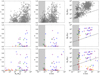 |
Fig. 14 Same as Fig. 5, but with the pebble accretion efficiency ϵOL18 from Ormel & Liu (2018). Only Discs 2, 5, and 8 are used here. The overall distributions are similar to Fig. 5, but giant planets are formed mostly with high metallicities [Fe/H] ≳ 0.3 (see text forfurther discussion). |
4.2 Formation of hot Jupiters
Any HJ formation model needs to explain that (1) HJs tend not to have nearby companions (e.g. Wright et al. 2009; Steffen et al. 2012; Huang et al. 2016), and (2) planets around higher metallicity stars tend to have a wider range of eccentricities (e.g. Dawson & Murray-Clay 2013; Shabram et al. 2016; Buchhave et al. 2018). Our simulations naturally explain both of these trends.
When HJs are formed via the tidal circularisation of highly eccentric orbits, the underlying assumption is that planetary systems have undergone some sort of dynamical evolution that increased eccentricities, such as planet-planet scattering (e.g. Ford & Rasio 2008; Chatterjee et al. 2008; Jurić & Tremaine 2008), the secular chaos (e.g. Wu & Lithwick 2011), or the Kozai-Lidov mechanism (e.g. Fabrycky & Tremaine 2007; Naoz 2016). The evolution of such planets often removes neighbouring planets, and the resulting HJs tend to be alone and have a range of eccentricities and inclinations. In our simulations, these HJs often belong to high-metallicity and/or massive discs, which typically produce a few giant planets that are prone to dynamical instabilities. On the other hand, when HJs form in situ (i.e. via the migration of cores followed by gas accretion in our simulations), they often belong to low-metallicity discs, which typically produce 1–2 giant planets. Therefore, the resulting HJs tend to be alone and have low eccentricities and inclinations due to damping by the disc. HJs can also be formed in situ or via migration in high-metallicity discs. Such discs usually form multiple giant planets initially, including HJs, WJs, and CJs, but HJs and/or WJs are often removed via dynamical instabilities later on, leaving either (i) only CJs, or (ii) HJs and CJs (also see Mustill et al. 2015). Therefore, even in these cases, HJs usually have no neighbouring giant planets (but could be accompanied by CJs further out).
There may be some difficulties for the scenario in which HJs are formed in situ, in particular in low-metallicity discs. First, gas accretion may be stalled near the central stars, because the gas envelope becomes nearly isothermal and the timescale of replenishing the atmosphere with the disc gas becomes shorter than the Kelvin-Helmholtz gas accretion timescale (e.g. Ormel et al. 2015a,b; Ali-Dib et al. 2020). However, the gas accretion may still be possible when the disc is heated by the stellar radiation alone and temperature and entropy in the inner disc region is low (Ali-Dib et al. 2020), which may be the case towards the end of the disc’s lifetime. Second, the near-infrared disc fraction study by Yasui et al. (2010) suggested that the disc fraction of the low metallicity clusters declines within 1 Myr as opposed to several Myr for the solar-metallicity clusters. If the trend were to be confirmed by longer-wavelength studies, this may place a strong constraint on planet formation timescales in the low-metallicity environments. In our simulations, giant planets could be formed within ~ 1 Myr even in the low-metallicity discs as long as disc masses are high enough (see Fig. 8), but the disc’s lifetimes are much longer than that. Since our current studies do not take account of the feedback of the planets onto discs, the future study needs to investigate this further.
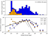 |
Fig. 15 Top: distribution of orbital periods of giant planets at the end of the simulations (blue) and those of giant planets whose orbits are tidally evolved for 3 Gyr (orange, see Sect. 3.1.2). Bottom: corresponding occurrence rates of giant planets as a function of orbital period. The blue symbols only include simulated giant planets, while the orange ones include both simulated and tidally evolved giant planets. The rates are calculated for the number of planets per star per Δ log P = 0.23 to be compared with Fig. 3 of Winn (2018). The black slopes are occurrence rates estimated from observed planets. The solid, dashed, dotted, and dot-dashed lines correspond to d n∕d ln P ∝ P0.26 ± 0.1 for giant planets with >0.3 MJ within 2000 days from Cumming et al. (2008), |
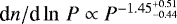
Numbers and fractions of HJs, WJs, CJs, and SCJs as defined in the semi-major axis range shown.
4.3 Upper limits on masses and planet formation radii
It is unclear what the maximum planetary mass generated by the core accretion scenario would be. Recently, Schlaufman (2018) pointed out that giant planets with ≲4 MJ tend to be around metal-rich dwarfs, while the same trend is not observed for ≳ 10 MJ. He suggested that these two distinct populations may correspond to core accretion and gravitational instability scenarios, with a transition mass being ~ 4–10 MJ. The transition mass is also comparable to planetary masses generated by the gravitational instability (≳3–5 MJ) that are reported in the semi-analytic studies (e.g. Kratter et al. 2010; Forgan & Rice 2011) and the numerical studies (e.g. Stamatellos & Whitworth 2008; Hall et al. 2017). Most of our simulations do not generate planets above ~ 10 MJ, and planetary masses of ~20 MJ were only found in massive, long-lived discs (Disc 7). As discussed in Sect. 2.3, it will probably be difficult to go above ~ 50 MJ with our model. Thus, although the highest-mass planets or brown dwarfs may be formed by gravitational instability, there is probably a significant overlap for masses of bodies both scenarios can generate.
How far away a planet can be formed via core accretion is not well understood either. In this work, we did not place planetary cores beyond ~20 au because pebble accretion becomes inefficient for a Ceres-size planetesimal to grow in the outer disc in our model (see Sect. 2.3). However, as we also show in Sect. 2.3, pebble accretion may still lead to giant planet formation out to and beyond 100 au if much larger planetesimals form there. If there are massive enough planetesimals available, pebble accretion (along with planetesimal accretion) may allow the growth of giant planets far beyond 20 au. Recent disc observations including ALMA regularly find gaps and rings over a wide range of disc radii, which may be attributed to growing planets (e.g. Zhang et al. 2016; Huang et al. 2018; Long et al. 2018). Lodato et al. (2019) estimated planetary masses from 48 observed gaps located around ~ 10− 130 au and found planetary masses ranging from 10−3 MJ ~ 0.3 M⊕ to over 10 MJ. If these gaps are indeed signposts of planets, the fact that a range of planetary masses is observed in the outer disc may indicate that core accretion is active out to these radii because gravitational instability is unlikely to form lower end mass planets. There is, however, a discrepancy between the frequency of observed SCJs (<4.1 for FGK stars, Bowler 2016) and the factthat the substructures such as rings and gaps are ubiquitous among observed discs (e.g. Andrews et al. 2018; Huang et al. 2018). Thus, if all of these rings and gaps correspond to planets, such planets would have to be removed from the outer disc region efficiently. This could be achieved if forming planets are redistributed due to migration (Lodato et al. 2019) or removed due to episodic accretion to the star (Brittain et al. 2020). The future studies should investigate the connection between forming planets and evolving protoplanetary discs further.
4.4 Formation of super cold Jupiters
In Sect. 3.1.3, we discuss two different pathways of forming SCJs via core accretion: (1) SCJs form in situ, either directly in the outer disc or via scattering of protoplanetary cores to the outer disc followed by gas accretion there (e.g. Kikuchi et al. 2014), or (2) giant planets first form within ~ 20 au and are then scattered into the outer disc. These two different scenarios are likely to lead to different distributions of physical and orbital parameters.
First, the in situ formation scenario of SCJs may lead to the a − Mp correlation where the planetary mass increases with the semi-major axis, because the disc aspect ratio increases with a, and thus the critical gap-opening mass for giant planets also becomes higher (Ida et al. 2013). On the other hand, the formation-then-scattering scenario might lead to an opposite trend because a lower-mass planet is more easily scattered further. We checked the Spearman’s rank correlation for simulated giant planets beyond 1 au (see the left panel of Fig. 11) and found the correlation coefficient of rs ~−0.18 with the p-value of p = 0.011 (rs ~−0.19 with the p-value of p = 0.0015 for all). Since the critical value for p < 0.05 is ∣ rs∣ ~ 0.2 for the size of our data, there is little or very weak negative correlation between the semi-major axis and the mass for giant planets. Due to the observational bias for high-mass planets, it is difficult to assess whether there is any trend for observed planets.
Second, the eccentricity distributions may also be different between these two scenarios. The scenario is likely to lead to an isolated eccentric giant planet, while the in situ formation scenario is more likely to lead to single- or multiple-giant planets on nearly circular orbits. In our simulations, giant planets scattered beyond 20 au have eccentricities ranging from e ~ 0.2–0.8 with the mean value of 0.56 (see Fig. 5). Kikuchi et al. (2014), on the other hand, showed that the eccentricity of the scattered core is reduced to e < 0.2 before reaching the Saturn mass via gas accretion in the outer disc. The eccentricities of multiple giant planets could increase via dynamical instabilities after formation, as long as they are not too far from each other (e.g. Chatterjee et al. 2008).
Recently, Bowler et al. (2020) studied the eccentricity distributions of 18 brown dwarfs (15–75 MJ) and nine giant planets (2–15 MJ) with orbital radii 5–100 au, and they found that the estimated eccentricity distribution is very broad and ranges over e = 0–1 for brown dwarfs and is much narrower with a peak at ē = 0.13 for giant planets, which may support the in situ formation scenario of SCJs more than the formation-then-scattering one. However, the peak eccentricity becomes ē = 0.23 for five giant planets excluding four HR 8799 planets on nearly circular orbits. The future observations will further constrain the eccentricity distribution and provide us with an important clue regarding the formation pathways of SCJs.
4.5 Mass fractions and metal contents
The left panel of Fig. 16 shows fractions of a planetary mass in the core (blue) and in the envelope (orange) for all the simulated planets. The envelope should usually also contain some metals, but here we added all the accreted dust particles to the core mass. Also plotted are the fitted metal-mass fractions of extrasolar planets from Thorngren et al. (2016; dashed line) and the estimated metal fractions in Jupiter, Uranus, and Neptune (stars with error bars, Fortney & Nettelmann 2010; Helled et al. 2020). As we can see, mass fractions of planetary cores of our simulations are lower than the estimate by Thorngren et al. (2016) by a factor of a few or more, though the distribution is consistent with the estimated metal-mass fraction of Jupiter.
This underestimation of the metal-mass fractions in our simulations may result from our assumption of gas accretion. For our simulations, the core mass and the envelope mass become comparable to each other: Mcore ~ Menv when Mp~ 4 ME. As seen in the figure, this is much lower than the crossover mass expected from the observed planets (~ 15 ME). The crossover mass represents a group of planets that are on the verge of becoming giant planets but failed to do so because the gas disc dissipated (i.e. tdiff ~ τKH):
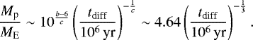 (49)
(49)
In Matsumura et al. (2017), the crossover mass was Mcore ~ Menv ~ 10 M⊕ as seen in Fig. 11, where we adopted (b, c) = (9, 3) rather than (8, 3). Thus, it is likely that we need to adopt (b, c) = (9, 3) to form planets with more appropriate rock-gas mass ratios. The reason why we adopted (b, c) = (8, 3) instead was to speed up gas accretion and to avoid the loss of planets due to type I migration. As discussed in Sect. 2.1, the pebble isolation mass is reached before the mass of migration transition from type I to type II. Therefore, the gas accretion timescale in this phase needs to be short compared to the migration timescale for a growing planet to switch from type I to type II regime. This further confirms the need for a proper mechanism of type I migration.
The right panel of Fig. 16 compares the mass-metallicity relation for simulated (circles) and observed (crosses) giant planets. The apparent lack of simulated planets with ~ 0.1–1 MJ for the solar metallicity case is most likely due to the choice of disc models rather than the real feature, because planets of this mass range are undergoing rapid gas accretion and have difficulties in forming unless the formation timescale is comparable to the disc dissipation timescale. There is an indication that the maximum masses of giant planets may increase for higher metallicity environments or even peak near [Fe/H] ~ 0, which is also observed by planetesimal accretion work by Mordasini et al. (2012). Otherwise, as stated in Sect. 3.1.2, masses of giant planets do not strongly depend on stellar metallicities. Thorngren et al. (2016) studied RV and transit planets and found a similar overall trend in the mass-metallicity relation (see their Fig. 9).
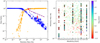 |
Fig. 16 Left: mass fractions of the rocky core (blue) |


4.6 Planetesimal accretion and pebble accretion
Planet formation via planetesimal accretion has been studied and compared with observed systems by many groups (e.g. Ida & Lin 2004; Ida et al. 2013; Mordasini et al. 2009, 2012; Thommes et al. 2008; Coleman & Nelson 2016a). Here, we compare our pebble accretion work with that of Mordasini et al. (2012) and Ida et al. (2013). Although a direct comparison is difficult, we discuss a few similarities and differences in planet formation outcomes.
Mordasini et al. (2012) used the single-planet formation population synthesis model and studied the effects of the disc’s metallicity, mass, and lifetime; while Ida et al. (2013) used a similar population synthesis model but took the effects of multiple-planet formation and dynamical interactions into account. The disc properties adopted in these studies are different, but they do overlap with ours. We considered the disc radii over 0.1–100 au with disc masses 0.02–0.2 M⊙ as well as stellar metallicities [Fe/H] = [−0.5, 0.5]. Mordasini et al. (2012) considered the disc outer radii of 30 au with disc masses 0.004–0.09 M⊙ and metallicities [Fe/H] = [−0.5, 0.5]. Applying their surface massdensity out to 100 au, the disc masses become 0.008–0.16 M⊙. Ida et al. (2013), on the other hand, considered the disc outer radii of 30 au with disc masses 1.6 × 10⁻⁴ − 0.16 M⊙ and metallicities [Fe/H] = [−0.2, 0.2]. Again, applying their surface mass density to the disc out to 100 au, the disc masses correspond to 0.0053–0.53 M⊙.
First, we highlight the difference in dependences of planet formation rates on disc properties such as metallicities, masses, and dissipation timescales. In terms of these disc parameters, the pebble mass accretion rate has the following dependency (see Eqs. (25), (14), and (16)):
![\begin{equation*} \dot{M}_{\textrm{core}}\,{=}\,\epsilon\dot{M}_{\textrm{F}}\propto\left(10^{\textrm{[Fe/H]}}\right)^{2}\alpha_{\textrm{acc}}^{-1}\dot{M}_{*}\propto\left(10^{\textrm{[Fe/H]}}\right)^{2}M_{\textrm{D}},\end{equation*}](/articles/aa/full_html/2021/06/aa39210-20/aa39210-20-eq95.png) (50)
(50)
where MD is the disc mass and the function of both the initial disc mass MD,0 and the dissipation timescale tdiff. On the other hand, a similar equation for planetesimal accretion is proportional to the dust surface mass density Σd = 10[Fe/H]Σg and has the following dependency (Mordasini et al. 2012):
![\begin{equation*} \dot{M}_{\textrm{core,plsml}}\propto\Sigma_{\textrm{d}}\propto10^{\textrm{[Fe/H]}}M_{\textrm{D}}. \end{equation*}](/articles/aa/full_html/2021/06/aa39210-20/aa39210-20-eq96.png) (51)
(51)
Ida et al. (2013) took account of the gas drag effect on planetesimals (Kokubo & Ida 2002) and thus had a slightly different dependency of:
![\begin{equation*} \dot{M}_{\textrm{core,plsml}}\propto10^{\textrm{[Fe/H]}}M_{\textrm{D}}^{7/5}. \end{equation*}](/articles/aa/full_html/2021/06/aa39210-20/aa39210-20-eq97.png) (52)
(52)
Therefore, in both pebble and planetesimal accretion models, increasing either metallicity or disc mass makes planet formation more efficient. This complementary effect of the metallicity and the disc mass was also pointed out by Mordasini et al. (2012).
In pebble accretion, the metallicity effect is more significant than the disc mass effect, as seen in Eq. (50). More specifically, changing the metallicity effect by an order of magnitude (e.g. from [Fe/H] = -0.5 to 0.5 in 10[Fe/H]) has a much larger effect on the accretion rate than changing the disc mass by an order of magnitude (e.g. from 0.02 M⊙ to 0.2 M⊙). Indeed, Fig. 8 shows that the giant planet formation timescale is different by ~ 2 orders of magnitude for the same disc mass with [Fe/H] = −0.5 and 0.5, while the timescale is different by ~1 order of magnitude for the same metallicity with MD,0 = 0.02 M⊙ and 0.2 M⊙.
The final mass, on the other hand, is less affected by the stellar metallicity both in planetesimal accretion (Mordasini et al. 2012)and in pebble accretion, though the reasons may be slightly different. For pebble accretion, the metallicity does not greatly affect final masses, partly because the PIM is independent of the stellar metallicity (see Eq. (39)) and partly because the final planetary mass is determined by the disc-limited gas accretion and thus is controlled by the available gas disc mass. For planetesimal accretion, however, the isolation mass depends on the dust density and thus masses of low-mass planets or cores of giant planets are likely to be affected by metallicities. Similarly to us, both Mordasini et al. (2012) and Ida et al. (2013) assumed that gas accretion is limited by the disc supply towards the end:
![\[ \dot{M}_{\textrm{gas}}\propto\dot{M}_{*}\propto M_{\textrm{D}}, \]](/articles/aa/full_html/2021/06/aa39210-20/aa39210-20-eq98.png)
though we took the reduced surface mass density effect in the gap into consideration (Eq. (44)), as shown in Eq. (45). Thus, the final mass of giant planets in particular is likely determined by the balance between the disc mass and the disc dissipation timescale, rather than by the metallicity.
In our work, this can be seen in Fig. 9, where planetary masses are higher for the higher disc mass and for the longer diffusion timescale. We can also see that planetary masses are higher for the same initial disc mass if the dissipation time is longer (i.e. when the disc experiences the lower mass accretion rate for a longer period of time, rather than the higher mass accretion rate for a shorter period of time). On the other hand, planetary masses are similar for the same disc model with different metallicities (see Sect. 3.1.2 for the discussion on the increasing mass trend in a − Mp).
One major difference between pebble and planetesimal accretion is that the formation timescale of giant planets in pebble accretion is short compared to the disc’s lifetime over a range of disc radii (e.g. Lambrechts & Johansen 2012). This makes it easier for giant planets to form even in less-optimal environments such as lower-mass, lower-metallicity, and/or more rapidly dissipating discs. Furthermore, as is also discussed in Sect. 4.3, pebble accretion may allow giant planet formation far beyond the radii in which we placed the cores for our simulations.
Finally, our Fig. 5 can be compared with Fig. 8 of Ida et al. (2013). Although adopted models and initial conditions are very different between these two studies, both reproduce the observed Mp − e, a − e, and a − Mp distributions well and show similar trends in simulated distributions. Perhaps the main difference is that, compared to Ida et al. (2013), our work has produced more eccentric planets. Ida et al. (2013) reported that only ~ 10% of their planets have moderate eccentricities of e ≳ 0.2. In our work, ~ 26.2% of all simulated planets (bottom panels) and ~40.3% of observable planets (middle panels) have e ≥ 0.2, as opposed to ~42% of observed planets (top panels). Thus, our work agrees much better with observations, at least for eccentricities (also see Fig. 6).
There may be a few factors leading to this difference. The dynamical instabilities generally require a few giant planets that are close enough to each other (e.g. Chatterjee et al. 2008). Ida et al. (2013) adopted planetesimal accretion, which is slower than pebble accretion, and therefore it may have been more difficult to form multiple giant planets nearby, because the inner one may have migrated inward and away from outer-growing protoplanets. Ida et al. (2013) did not take account of secular perturbations between giant planets in their Monte Carlo method for planet-planet scattering either, which can also trigger orbital instabilities and is of course automatically included in our N-body simulations.Furthermore, Ida et al. (2013) explored a relatively narrow range of metallicities of [Fe/H] = [−0.2, 0.2] as opposed to our [Fe/H] = [−0.5, 0.5]. Since the number of giant planets per system is more sensitive to disc masses for lower metallicities (e.g. see cases with [Fe/H] ≲ 0.0 in Fig. 7), they may have generated a lower number of giant planets per system on the average. Although, this effect may have been mitigated to an extent since they covered a wide range of disc masses (spanning two orders of magnitude), and the low metallicities can be compensated for by more massive discs. Also, it is possible that the eccentricity damping effect was too strong in their simulations, which prevented the occurrence of dynamical instabilities (see next sub-section as well as Bitsch et al. 2020).
4.7 Comparison with Bitsch et al. (2019)
Here, we briefly compare our work with a similar N-body work on giant planet formation by Bitsch et al. (2019). A direct comparison is not possible since the details of their models are different from ours (e.g. e-quation of motion, pebble and gas accretion models, pebble isolation mass). However, we list differences in disc parameters below and compare their results with ours for similar disc parameters. We find that there are both similarities and differences.
Their gas accretion rate follows Hartmann et al. (1998) and Bitsch et al. (2015), and it is the same as the formula adopted by Matsumura et al. (2017):
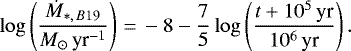 (53)
(53)
Although we did not use the formula for this paper, their accretion rate very closely follows Disc 2 of our model (which corresponds to Md = 0.06 M⊙ with tdiff = 0.1 Myr and thus αacc ~ 7.4 × 10⁻²). Since they evolve the disc from 2 Myr to 5 Myr, their mass accretion changes from Ṁ* ~ 3.8 × 10⁻⁹ M⊙ to ~ 1 × 10⁻⁹ M⊙. They also adopted αacc = 5.4 × 10⁻³ for disc accretion and αturb = 5.4 × 10⁻⁴ and 10−4 for disc turbulence. Although the mass evolution is similar to our Disc 2, their disc could be close to our Disc 6 (i.e. Md = 0.02 M⊙ with tdiff = 1 Myr and thus αacc ~ 7.4 × 10⁻³) since they started with an evolved disc and assumed αacc = 5.4 × 10⁻³. In our simulations, both produce similar types of planets (see Fig. 9 and a discussion below).
On the other hand, their pebble mass flux is
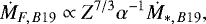 (54)
(54)
where Z = 1% is the metallicity. Although they assumed the solar metallicity for their simulations, they scaled the pebble mass flux by the factor of Speb = 1–10, which corresponds to exploring the metallicities of [Fe/H] = 0.0 to 0.43. Since our pebble mass flux is ṀF ∝ Z2α−1Ṁ*, the dependence on each parameter is similar.
One of the conclusions by Bitsch et al. (2019) was that formation of CJs was possible for cores originating from 10 au with αturb = 5.4 × 10⁻⁴ and those from 5 au with αturb = 10−4. From their Figs. 4–6, the formation of giant planets up to ~300 M⊕ was possible for both αturb cases above Speb = 2.5 (which corresponds to [Fe/H] ≳ 0.17), while no giant planets formed for the solar metallicity case. Our simulations show similar trends. In Disc 6 with αturb = 10−4, giant planets primarily become low-mass CJs with ~ 100–400 M⊕ for metallicities [Fe/H] = 0.3 and 0.5, while no giant planets form for [Fe/H] ≤ 0.0 (see Fig. 9). In Disc 2, the outcomes are similar except that planetary masses are lower ~ 100–300 M⊕, and very low-mass giant planets can be formed with [Fe/H] = 0.0 (but not for lower metallicities). Out of formed giant planets, those starting from 3–5 au typically become the closest-in CJs with orbital radius beyond ~1 au. For higher (lower) αturb, planets tend to migrate further (less) (see Sect. 3.2.1 and Fig. 12) as indicated by Bitsch et al. (2019).
One major difference between Bitsch et al. (2019) and our work is that their simulations are left with a number of giant planets with low eccentricities, while we have successfully reproduced the eccentricity distribution of giant planets (see Fig. 5). The result may be surprising at a glance because the number of giant planets that formed and survived in simulations by Bitsch et al. (2019) is higher than in our simulations, and typically ~ 5 or more from their Figs. 6 and 7. We note that the higher number of surviving planets is not likely due to the difference in the initial number of cores (60 for their simulations as opposed to 10 for ours). Jurić & Tremaine (2008) showed that, even when there were 50 giant planets, the final number of planets would be 2–3, as long as the dynamical instabilities occur. The eccentricity distribution from such simulations with an initially high number of giant planets agrees well with observations, and also with dynamical instability simulations with lower number of giant planets (e.g. Jurić & Tremaine 2008; Chatterjee et al. 2008). Thus, the large number of surviving giant planets in Bitsch et al. (2019) indicates that the dynamical instability among giant planets was rare in their simulations. Indeed, even their long-term evolution of 100 Myr did not lead to a dramatic increase in orbital eccentricities (Bitsch et al. 2019).
While this manuscript was under revision, we became aware of the work by Bitsch et al. (2020), in which they studied the effects of eccentricity and inclination damping efficiencies on the eccentricity distribution of giant planets. They parameterised the eccentricity and inclination damping timescales as τa = K τe = K τi with K = 5, 50, 500, and 5000, and found that the observed eccentricity distribution of giant planets can be recovered for slow damping with K ~ 5–50. Since Bitsch et al. (2019) adopted a faster damping with K = 100, it may be the reason why they did not obtain eccentric giants.
As seen in Fig. 1, we also have K ~ 100, though we managed to reproduce the eccentricity distribution of giants. Since our eccentricity and inclination damping prescriptions are similar to those by Bitsch et al. (2019), it is possible that subtle differences in disc conditions changed the dynamical outcomes of simulations. For example, the choice of αacc = 5.4 × 10⁻³ in Bitsch et al. (2019) may be inconsistent with the time evolution of the stellar mass accretion rate they adopted (Eq. (53)). The fit to this observed mass accretion rate requires a rather high viscosity αacc ~ 0.01 for the discsize of 10–100 au (Hartmann et al. 1998) and even higher αacc for a larger disc. By assuming the lower αacc for the sameaccretion rate, the estimated surface mass density and thus the disc mass becomes higher, which leads to more efficient eccentricity and inclination damping. In fact, we observed a similar lack of dynamical instabilities in the no-migration simulations of Matsumura et al. (2017) — we adopted the same stellar mass accretion equation as Eq. (53) and used α ≤5 × 10⁻³ when 3–5 giant planets were formed (except for one case with 3 giant planets with α = 0.01). For completeness, Matsumura et al. (2017) had K ~ 100 in the type I regime and K ~ 10 in the type II regime, which should favour more eccentric systems. Moreover, we had twice as many cores in a much narrower range of disc radii (0.3–5 au) compared to the current runs. It is possible, however, since these simulations did not include migration, that planets were separated too far from one another to invoke dynamical instabilities within simulation times. In that case, convergent migration may also play an important role in determining the eccentricity and inclination distributions of planetary systems.
5 Conclusion
For this paper, we studied the formation of planetary systems via pebble accretion by using N-body simulations, and we investigated the effects of disc parameters such as masses, dissipation timescales, and metallicities. This is a continuation of Matsumura et al. (2017), in which we modified the N-body code SyMBA (Duncan et al. 1998) to incorporate the pebble accretion model by Ida et al. (2016), gas accretion, type I and type II migration, and eccentricity and inclination damping. In this work, we updated the code as detailed in Sect. 2 to take account of the recent development of the field, and we also adopted a two-α disc model, where mass accretion and disc turbulence have different drivers.
We find that the disc masses, dissipation timescales, and stellar metallicities all affect the efficiency of planet formation. The effects of each parameter can be summarised as follows (see Sect. 4.6):
-
Disc metallicities [Fe/H] affect the formation timescales of protoplanetary cores, but they do not strongly affect the final planetary masses.
-
Initial disc masses MD,0 affect both core formation and gas accretion timescales, and thus the final planetary masses.
-
Disc diffusion timescales tdiff set time limits on planet formation in the disc, and thus affect the final planetary masses.
We identified two types of giant planet formation trends, depending on whether planet formation is fast compared to the disc’s dispersal or not. When a disc’s dissipation timescales are long in comparison to typical planet formation timescales (Discs 4, 5, 7, and 8 in our simulations, formation-dominated case), giant planets are massive (~ MJ or higher) and distributed over a wide range of orbital radii (from ~0.1 au to over 100 au). On the other hand, when a disc’s dissipation timescales are comparable to planet formation timescales (Discs 1, 2, 3, and 6, disc-dissipation-limited case), giant planets tend to be low-mass (~ MJ or lower) and CJs (with a ≳ 1 au). The formation timescale depends both on stellar metallicities and disc masses — the timescale is shorter for more massive, more metal-rich discs. Therefore, protoplanetary cores tend to migrate significantly before accreting gas to become giant planets in low metallicity discs, while giant planets can form in situ in the outer part of high-metallicity, massive discs. For low-mass, low-metallicity discs, giant planet formation is difficult.
Our main findings are the following:
-
Differently from Matsumura et al. (2017), we successfully reproduced the overall distribution trends of semi-major axes a, eccentricities e, and planetary masses Mp of extrasolar giant planets (see Sect. 3.1.1 and Fig. 5), though we tend to overproduce CJs compared to HJs and WJs. The success of reproducing the a − Mp distribution, especially for CJs, is largely due to the new type II migration formula and the two-α disc model, as proposed by Ida et al. (2018). The success in reproducing the e distribution is likely due to a more self-consistent disc model, a higher number of giant planets formed per system compared to Matsumura et al. (2017), and not too efficient eccentricity and inclination damping in the disc (see Sect. 4.7).
-
The overall occurrence rates of giant planets as a function of orbital periods agree well with observed trends (see Sect. 4.1). The occurrence rates increase with periods in the inner region, decrease in the outer region, and peak at ~1–10 au. The most abundant giant planets are CJs (>50%), and thus more than half the giant planets in our simulations stay near their formation region.
-
As discussed in Sect. 4.2, our simulations naturally explain why HJs tend to be alone (e.g. Wright et al. 2009; Steffen et al. 2012; Huang et al. 2016), and also why the eccentricities of HJs are low around low-metallicity stars and vary more widely around high-metallicity ones (e.g. Dawson & Murray-Clay 2013; Shabram et al. 2016; Buchhave et al. 2018). The same trend is expected for stellar obliquities of their host stars, and the current observations support that (see Sect. 3.1.2).
-
In low-metallicity discs, HJs tend to form in situ: protoplanetary cores migrate to the inner disc and accrete gas there. This is because planet formation is slower in the low-metallicity discs, which leads to greater migration of a protoplanetary core before it reaches the PIM and starts accreting a significant gas to become a giant planet. Since the low-metallicity discs tend to form just 1–2 giant planets, HJs tend to be alone and on nearly circular and coplanar orbits.
-
In high-metallicity discs, HJs can be formed either via tidal circularisation of highly eccentric orbits or via a migration scenario (including in situ formation; see Sect. 3.1.2). The higher metallicity discs tend to produce a number of giant planets that are prone to dynamical instabilities. A HJ could be formed from a WJ/CJ as its eccentric orbit is circularised. Alternatively, HJs could be first formed in situ (i.e. via core migration followed by gas accretion) or via migration, along with WJs and CJs. The dynamical instabilities in such systems often remove either HJs and/or WJs, leaving either (i) only CJs, or (ii) HJs with CJs. HJs formed in high-metallicity discs have a wider variety of eccentricities and inclinations and also tend to be alone.
-
-
If an SCJ is formed, as a giant planet grows within ~20 au and then gets scattered outward, we expect that such an SCJ (1) was born in a high-metallicity disc (
![$\left[\textrm{Fe/H}\right]\gtrsim0.0$](/articles/aa/full_html/2021/06/aa39210-20/aa39210-20-eq101.png) ), (2) has an eccentric orbit, and (3) tends to be accompanied by another giant planet (~80%) (see Sect. 3.1.3).
), (2) has an eccentric orbit, and (3) tends to be accompanied by another giant planet (~80%) (see Sect. 3.1.3). -
Most warm Jupiters (0.1 au ≲ a ≲ 1 au) are formed in the formation-dominated discs (i.e. Discs 4, 5, 7, and 8 in our simulations). In other words, in our simulations, it is difficult to form WJs in rapidly dissipating, low-mass and/or low-metallicity discs.
-
CJs tendto be formed in high-mass and/or high-metallicity discs, where the planet formation timescale is comparable to or shorter than the disc dissipation timescale.
Finally, there are still several issues that need to be resolved/explored in our work. Most importantly, type I migration is still too fast and we tendto lose SEs. For example, type I migration can be slowed in the inner disc region if we fully adopt the wind-driven disc, as in Ogihara et al. (2018). Resolving the migration issue is also important when choosing a more appropriate gas accretion formula, which would provide more accurate planetary compositions (see Sect. 4.5). Furthermore, when αturb ≪ αacc as we assumed, the gap depth may also be affected by the wind-driven accretion.
Acknowledgements
We thank Man Hoi Lee and Eduard Vorobyov for useful discussions and an anonymous referee for detailed comments. SM is grateful to Aurora Sicilia-Aguilar for valuable discussions and also for kindly sharing her data from Sicilia-Aguilar et al. (2010). SM would also like to thank the Earth-Life Science Institute at Tokyo Institute of Technology for its hospitality, where part of this work has been done. SM is partly supported by the STFC grant number ST/S000399/1 (The Planet-Disk Connection: Accretion, Disk Structure, and Planet Formation). RB acknowledges financial assistance from the Japan Society for the Promotion of Science (JSPS) Shingakujutsu Kobo (JP19H05071). SI is supported by MEXT Kakenhi 18H05438.
References
- Adachi, I., Hayashi, C., & Nakazawa, K. 1976, Prog. Theor. Phys., 56, 1756 [NASA ADS] [CrossRef] [Google Scholar]
- Ali-Dib, M., Cumming, A., & Lin, D. N. C. 2020, MNRAS, 494, 2440 [Google Scholar]
- Andrews, S. M., & Williams, J. P. 2007, ApJ, 659, 705 [NASA ADS] [CrossRef] [Google Scholar]
- Andrews, S. M., Wilner, D. J., Hughes, A. M., Qi, C., & Dullemond, C. P. 2010, ApJ, 723, 1241 [Google Scholar]
- Andrews, S. M., Huang, J., Pérez, L. M., et al. 2018, ApJ, 869, L41 [Google Scholar]
- Ataiee, S., Baruteau, C., Alibert, Y., & Benz, W. 2018, A&A, 615, A110 [NASA ADS] [CrossRef] [EDP Sciences] [Google Scholar]
- Bai, X.-N. 2016, ApJ, 821, 80 [Google Scholar]
- Bai, X.-N. 2017, ApJ, 845, 75 [Google Scholar]
- Bai, X.-N., & Stone, J. M. 2013, ApJ, 769, 76 [Google Scholar]
- Balbus, S. A., & Hawley, J. F. 1998, Rev. Mod. Phys., 70, 1 [Google Scholar]
- Baron, F., Lafrenière, D., Artigau, É., et al. 2019, AJ, 158, 187 [Google Scholar]
- Batygin, K., Bodenheimer, P. H., & Laughlin, G. P. 2016, ApJ, 829, 114 [Google Scholar]
- Birnstiel, T., Klahr, H., & Ercolano, B. 2012, A&A, 539, A148 [NASA ADS] [CrossRef] [EDP Sciences] [Google Scholar]
- Bitsch, B., Lambrechts, M., & Johansen, A. 2015, A&A, 582, A112 [NASA ADS] [CrossRef] [EDP Sciences] [Google Scholar]
- Bitsch, B., Morbidelli, A., Johansen, A., et al. 2018, A&A, 612, A30 [NASA ADS] [CrossRef] [EDP Sciences] [Google Scholar]
- Bitsch, B., Izidoro, A., Johansen, A., et al. 2019, A&A, 623, A88 [NASA ADS] [CrossRef] [EDP Sciences] [Google Scholar]
- Bitsch, B., Trifonov, T., & Izidoro, A. 2020, A&A, 643, A66 [EDP Sciences] [Google Scholar]
- Boley, A. C., Granados Contreras, A. P., & Gladman, B. 2016, ApJ, 817, L17 [NASA ADS] [CrossRef] [Google Scholar]
- Bowler, B. P. 2016, PASP, 128, 102001 [NASA ADS] [CrossRef] [Google Scholar]
- Bowler, B. P., Blunt, S. C., & Nielsen, E. L. 2020, AJ, 159, 63 [Google Scholar]
- Brasser, R., Bitsch, B., & Matsumura, S. 2017, AJ, 153, 222 [NASA ADS] [CrossRef] [Google Scholar]
- Brasser, R., Matsumura, S., Muto, T., & Ida, S. 2018, ApJ, 864, L8 [Google Scholar]
- Brittain, S. D., Najita, J. R., & Carr, J. S. 2019, ApJ, 883, 37 [CrossRef] [Google Scholar]
- Brittain, S. D., Najita, J. R., Dong, R., & Zhu, Z. 2020, ApJ, 895, 48 [CrossRef] [Google Scholar]
- Bryan, M. L., Knutson, H. A., Howard, A. W., et al. 2016, ApJ, 821, 89 [NASA ADS] [CrossRef] [Google Scholar]
- Buchhave, L. A., Bitsch, B., Johansen, A., et al. 2018, ApJ, 856, 37 [NASA ADS] [CrossRef] [Google Scholar]
- Casassus, S., & Pérez, S. 2019, ApJ, 883, L41 [CrossRef] [Google Scholar]
- Chambers, J. E. 2016, ApJ, 825, 63 [Google Scholar]
- Chatterjee, S., Ford, E. B., Matsumura, S., & Rasio, F. A. 2008, ApJ, 686, 580 [Google Scholar]
- Chiang, E., & Laughlin, G. 2013, MNRAS, 431, 3444 [Google Scholar]
- Coleman, G. A. L., & Nelson, R. P. 2014, MNRAS, 445, 479 [NASA ADS] [CrossRef] [Google Scholar]
- Coleman, G. A. L., & Nelson, R. P. 2016a, MNRAS, 460, 2779 [NASA ADS] [CrossRef] [Google Scholar]
- Coleman, G. A. L., & Nelson, R. P. 2016b, MNRAS, 457, 2480 [Google Scholar]
- Cumming, A., Butler, R. P., Marcy, G. W., et al. 2008, PASP, 120, 531 [CrossRef] [Google Scholar]
- Dawson, R. I., & Murray-Clay, R. A. 2013, ApJ, 767, L24 [NASA ADS] [CrossRef] [Google Scholar]
- Duffell, P. C., & MacFadyen, A. I. 2013, ApJ, 769, 41 [NASA ADS] [CrossRef] [Google Scholar]
- Duncan, M. J., Levison, H. F., & Lee, M. H. 1998, AJ, 116, 2067 [NASA ADS] [CrossRef] [EDP Sciences] [Google Scholar]
- Fabrycky, D., & Tremaine, S. 2007, ApJ, 669, 1298 [Google Scholar]
- Fendyke, S. M., & Nelson, R. P. 2014, MNRAS, 437, 96 [Google Scholar]
- Fernandes, R. B., Mulders, G. D., Pascucci, I., Mordasini, C., & Emsenhuber, A. 2019, ApJ, 874, 81 [Google Scholar]
- Ford, E. B., & Rasio, F. A. 2008, ApJ, 686, 621 [NASA ADS] [CrossRef] [Google Scholar]
- Forgan, D., & Rice, K. 2011, MNRAS, 417, 1928 [NASA ADS] [CrossRef] [Google Scholar]
- Fortney, J. J., & Nettelmann, N. 2010, SSRv, 152, 423 [Google Scholar]
- Fung, J., Shi, J.-M., & Chiang, E. 2014, ApJ, 782, 88 [NASA ADS] [CrossRef] [Google Scholar]
- Hall, C., Forgan, D., & Rice, K. 2017, MNRAS, 470, 2517 [NASA ADS] [CrossRef] [Google Scholar]
- Hartmann, L., Calvet, N., Gullbring, E., & D’Alessio, P. 1998, ApJ, 495, 385 [NASA ADS] [CrossRef] [Google Scholar]
- Helled, R., Nettelmann, N., & Guillot, T. 2020, SSRv, 216, 38 [Google Scholar]
- Huang, C., Wu, Y., & Triaud, A. H. M. J. 2016, ApJ, 825, 98 [Google Scholar]
- Huang, J., Andrews, S. M., Dullemond, C. P., et al. 2018, ApJ, 869, L42 [Google Scholar]
- Hueso, R., & Guillot, T. 2005, A&A, 442, 703 [NASA ADS] [CrossRef] [EDP Sciences] [Google Scholar]
- Hut, P. 1981, A&A, 99, 126 [NASA ADS] [Google Scholar]
- Ida, S., & Lin, D. N. C. 2004, ApJ, 604, 388 [NASA ADS] [CrossRef] [PubMed] [Google Scholar]
- Ida, S., & Lin, D. N. C. 2008, ApJ, 673, 487 [NASA ADS] [CrossRef] [Google Scholar]
- Ida, S., Lin, D. N. C., & Nagasawa, M. 2013, ApJ, 775, 42 [NASA ADS] [CrossRef] [Google Scholar]
- Ida, S., Guillot, T., & Morbidelli, A. 2016, A&A, 591, A72 [NASA ADS] [CrossRef] [EDP Sciences] [Google Scholar]
- Ida, S., Tanaka, H., Johansen, A., Kanagawa, K. D., & Tanigawa, T. 2018, ApJ, 864, 77 [NASA ADS] [CrossRef] [Google Scholar]
- Ida, S., Yamamura, T., & Okuzumi, S. 2019, A&A, 624, A28 [NASA ADS] [CrossRef] [EDP Sciences] [Google Scholar]
- Ida, S., Muto, T., Matsumura, S., & Brasser, R. 2020, MNRAS, 494, 5666 [Google Scholar]
- Ikoma, M., Nakazawa, K., & Emori, H. 2000, ApJ, 537, 1013 [NASA ADS] [CrossRef] [Google Scholar]
- Izidoro, A., Bitsch, B., Raymond, S. N., et al. 2021, A&A, in press, https://doi.org/10.1051/0004-6361/201935336 [NASA ADS] [CrossRef] [EDP Sciences] [Google Scholar]
- Johansen, A., & Lambrechts, M. 2017, Annu. Rev. Earth Planet. Sci., 45, 359 [Google Scholar]
- Johansen, A., Oishi, J. S., Mac Low, M.-M., et al. 2007, Nature, 448, 1022 [Google Scholar]
- Johansen, A., Youdin, A., & Mac Low, M.-M. 2009, ApJ, 704, L75 [Google Scholar]
- Johansen, A., Mac Low, M.-M., Lacerda, P., & Bizzarro, M. 2015, Sci. Adv., 1, 1500109 [Google Scholar]
- Johansen, A., Ida, S., & Brasser, R. 2019, A&A, 622, A202 [NASA ADS] [CrossRef] [EDP Sciences] [Google Scholar]
- Jurić, M., & Tremaine, S. 2008, ApJ, 686, 603 [NASA ADS] [CrossRef] [Google Scholar]
- Kanagawa, K. D., Tanaka, H., & Szuszkiewicz, E. 2018, ApJ, 861, 140 [NASA ADS] [CrossRef] [Google Scholar]
- Keppler, M., Benisty, M., Müller, A., et al. 2018, A&A, 617, A44 [NASA ADS] [CrossRef] [EDP Sciences] [Google Scholar]
- Kikuchi, A., Higuchi, A., & Ida, S. 2014, ApJ, 797, 1 [NASA ADS] [CrossRef] [Google Scholar]
- Kokubo, E., & Ida, S. 2002, ApJ, 581, 666 [Google Scholar]
- Kratter, K. M., Murray-Clay, R. A., & Youdin, A. N. 2010, ApJ, 710, 1375 [NASA ADS] [CrossRef] [Google Scholar]
- Kretke, K. A. & Levison, H. F. 2014, AJ, 148, 109 [NASA ADS] [CrossRef] [Google Scholar]
- Lambrechts, M., & Johansen, A. 2012, A&A, 544, A32 [CrossRef] [EDP Sciences] [Google Scholar]
- Lambrechts, M., & Johansen, A. 2014, A&A, 572, A107 [NASA ADS] [CrossRef] [EDP Sciences] [Google Scholar]
- Lambrechts, M., Johansen, A., & Morbidelli, A. 2014, A&A, 572, A35 [NASA ADS] [CrossRef] [EDP Sciences] [Google Scholar]
- Lambrechts, M., Morbidelli, A., Jacobson, S. A., et al. 2019, A&A, 627, A83 [NASA ADS] [CrossRef] [EDP Sciences] [Google Scholar]
- Levison, H. F., Kretke, K. A., & Duncan, M. J. 2015, Nature, 524, 322 [Google Scholar]
- Lin, D. N. C., & Papaloizou, J. 1986, ApJ, 309, 846 [NASA ADS] [CrossRef] [Google Scholar]
- Lin, D. N. C., & Papaloizou, J. C. B. 1993, Protostars and Planets III (The University of Arizona Press) [Google Scholar]
- Lin, D. N. C., Bodenheimer, P., & Richardson, D. C. 1996, Nature, 380, 606 [NASA ADS] [CrossRef] [Google Scholar]
- Lodato, G., Dipierro, G., Ragusa, E., et al. 2019, MNRAS, 486, 453 [NASA ADS] [CrossRef] [Google Scholar]
- Long, F., Pinilla, P., Herczeg, G. J., et al. 2018, ApJ, 869, 17 [NASA ADS] [CrossRef] [Google Scholar]
- Lynden-Bell, D., & Pringle, J. E. 1974, MNRAS, 168, 603 [NASA ADS] [CrossRef] [Google Scholar]
- Marzari, F., & Weidenschilling, S. J. 2002, Icarus, 156, 570 [Google Scholar]
- Matsumura, S., Peale, S. J., & Rasio, F. A. 2010, ApJ, 725, 1995 [Google Scholar]
- Matsumura, S., Brasser, R., & Ida, S. 2017, A&A, 607, A67 [NASA ADS] [CrossRef] [EDP Sciences] [Google Scholar]
- Mayor, M., Marmier, M., Lovis, C., et al. 2011, ArXiv e-prints [arXiv:1109.2497] [Google Scholar]
- Morbidelli, A.,& Nesvorny, D. 2012, A&A, 546, A18 [CrossRef] [EDP Sciences] [Google Scholar]
- Mordasini, C., Alibert, Y., & Benz, W. 2009, A&A, 501, 1139 [NASA ADS] [CrossRef] [EDP Sciences] [Google Scholar]
- Mordasini, C., Alibert, Y., Benz, W., Klahr, H., & Henning, T. 2012, A&A, 541, A97 [NASA ADS] [CrossRef] [EDP Sciences] [Google Scholar]
- Mustill, A. J., Davies, M. B., & Johansen, A. 2015, ApJ, 808, 14 [NASA ADS] [CrossRef] [Google Scholar]
- Muto, T., Takeuchi, T., & Ida, S. 2011, ApJ, 737, 37 [NASA ADS] [CrossRef] [Google Scholar]
- Nagasawa, M.,& Ida, S. 2011, ApJ, 742, 72 [Google Scholar]
- Nagasawa, M., Ida, S., & Bessho, T. 2008, ApJ, 678, 498 [Google Scholar]
- Naoz, S. 2016, ARA&A, 54, 441 [Google Scholar]
- Naoz, S., Farr,W. M., Lithwick, Y., Rasio, F. A., & Teyssandier, J. 2011, Nature, 473, 187 [Google Scholar]
- Nielsen, E. L., De Rosa, R. J., Macintosh, B., et al. 2019, AJ, 158, 13 [NASA ADS] [CrossRef] [Google Scholar]
- Ogihara, M., & Hori, Y. 2020, ApJ, 892, 124 [Google Scholar]
- Ogihara, M., Duncan, M. J., & Ida, S. 2010, ApJ, 721, 1184 [Google Scholar]
- Ogihara, M., Kokubo, E., Suzuki, T. K., Morbidelli, A., & Crida, A. 2017, A&A, 608, A74 [NASA ADS] [CrossRef] [EDP Sciences] [Google Scholar]
- Ogihara, M., Kokubo, E., Suzuki, T. K., & Morbidelli, A. 2018, A&A, 615, A63 [NASA ADS] [CrossRef] [EDP Sciences] [Google Scholar]
- Oka, A., Nakamoto, T., & Ida, S. 2011, ApJ, 738, 141 [NASA ADS] [CrossRef] [Google Scholar]
- Ormel, C. W., & Klahr, H. H. 2010, A&A, 520, A43 [NASA ADS] [CrossRef] [EDP Sciences] [Google Scholar]
- Ormel, C. W., & Kobayashi, H. 2012, ApJ, 747, 115 [NASA ADS] [CrossRef] [Google Scholar]
- Ormel, C. W., & Liu, B. 2018, A&A, 615, A178 [NASA ADS] [CrossRef] [EDP Sciences] [Google Scholar]
- Ormel, C. W., Kuiper, R., & Shi, J.-M. 2015a, MNRAS, 446, 1026 [NASA ADS] [CrossRef] [Google Scholar]
- Ormel, C. W., Shi, J.-M., & Kuiper, R. 2015b, MNRAS, 447, 3512 [Google Scholar]
- Paardekooper, S.-J., Baruteau, C., & Kley, W. 2011, MNRAS, 410, 293 [NASA ADS] [CrossRef] [Google Scholar]
- Pfalzner, S., Steinhausen, M., & Menten, K. 2014, ApJ, 793, L34 [NASA ADS] [CrossRef] [Google Scholar]
- Santerne, A., Moutou, C., Tsantaki, M., et al. 2016, A&A, 587, A64 [NASA ADS] [CrossRef] [EDP Sciences] [Google Scholar]
- Sato, T., Okuzumi, S., & Ida, S. 2016, A&A, 589, A15 [NASA ADS] [CrossRef] [EDP Sciences] [Google Scholar]
- Schlaufman, K. C. 2018, ApJ, 853, 37 [NASA ADS] [CrossRef] [Google Scholar]
- Shabram, M., Demory, B.-O., Cisewski, J., Ford, E. B., & Rogers, L. 2016, ApJ, 820, 93 [NASA ADS] [CrossRef] [Google Scholar]
- Shakura, N. I., & Sunyaev, R. A. 1973, A&A, 24, 337 [NASA ADS] [Google Scholar]
- Sicilia-Aguilar, A., Henning, T., & Hartmann, L. W. 2010, ApJ, 710, 597 [Google Scholar]
- Simon, J. B., Armitage, P. J., Li, R., & Youdin, A. N. 2016, ApJ, 822, 55 [NASA ADS] [CrossRef] [Google Scholar]
- Stamatellos, D., & Whitworth, A. P. 2008, A&A, 480, 879 [NASA ADS] [CrossRef] [EDP Sciences] [Google Scholar]
- Steffen, J. H., Ragozzine, D., Fabrycky, D. C., et al. 2012, Proc. Natl. Acad. Sci. U.S.A., 109, 7982 [NASA ADS] [CrossRef] [Google Scholar]
- Suzuki, T. K., Ogihara, M., Morbidelli, A. r., Crida, A., & Guillot, T. 2016, A&A, 596, A74 [NASA ADS] [CrossRef] [EDP Sciences] [Google Scholar]
- Tanaka, H., & Ward, W. R. 2004, ApJ, 602, 388 [Google Scholar]
- Tanaka, H., Murase, K., & Tanigawa, T. 2020, ApJ, 891, 143 [CrossRef] [Google Scholar]
- Tanigawa, T., & Tanaka, H. 2016, ApJ, 823, 48 [NASA ADS] [CrossRef] [Google Scholar]
- Thommes, E. W., Matsumura, S., & Rasio, F. A. 2008, Science, 321, 814 [NASA ADS] [CrossRef] [PubMed] [Google Scholar]
- Thorngren, D. P., Fortney, J. J., Murray-Clay, R. A., & Lopez, E. D. 2016, ApJ, 831, 64 [NASA ADS] [CrossRef] [Google Scholar]
- Tsukagoshi, T., Muto, T., Nomura, H., et al. 2019, ApJ, 878, L8 [Google Scholar]
- Tychoniec, Ł., Tobin, J. J., Karska, A., et al. 2018, ApJS, 238, 19 [NASA ADS] [CrossRef] [Google Scholar]
- Vicente, S. M., & Alves, J. 2005, A&A, 441, 195 [NASA ADS] [CrossRef] [EDP Sciences] [Google Scholar]
- Weidenschilling, S. J. 1977, MNRAS, 180, 57 [Google Scholar]
- Wimarsson, J., Liu, B., & Ogihara, M. 2020, MNRAS, 496, 3314 [Google Scholar]
- Winn, J. N. 2018, Planet Occurrence: Doppler and Transit Surveys, 195 [Google Scholar]
- Wright, J. T., Upadhyay, S., Marcy, G. W., et al. 2009, ApJ, 693, 1084 [NASA ADS] [CrossRef] [Google Scholar]
- Wu, Y., & Lithwick, Y. 2011, ApJ, 735, 109 [Google Scholar]
- Yasui, C., Kobayashi, N., Tokunaga, A. T., Saito, M., & Tokoku, C. 2010, ApJ, 723, L113 [NASA ADS] [CrossRef] [Google Scholar]
- Youdin, A. N., & Goodman, J. 2005, ApJ, 620, 459 [NASA ADS] [CrossRef] [Google Scholar]
- Zhang, K., Bergin, E. A., Blake, G. A., et al. 2016, ApJ, 818, L16 [NASA ADS] [CrossRef] [Google Scholar]
As seen in the figure, there is a possibility that the required gap depth becomes deeper than 50% for the PIM by Ataiee et al. (2018) as well. However, we confirm that within our simulation parameters, the effects are not important.
The number of cores is chosen arbitrarily. However, Bitsch et al. (2020) recently studied pebble accretion with 15, 30, and 60 cores across 3–17 au and found that the number of cores generally has little effect on the final outcome of planetary distributions. The exception is the case when the eccentricity and inclination damping are very slow so that the higher number of cores leads to more random orbits. Since the number of our cores is lower and they are distributed over a wider orbital range compared to their work, our initial conditions are less prone to dynamical instabilities compared to theirs.
All Tables
Numbers and fractions of HJs, WJs, CJs, and SCJs as defined in the semi-major axis range shown.
All Figures
|
Fig. 1 Comparison of evolution timescales of semi-major axis τa (blue), eccentricity τe (orange), and inclination τi (green) for a planet at 3.16 au with the circular and coplanar orbit in Disc 6. Solid and dashed blue lines are from Eqs. (8) and (3), respectively. The vertical black dashed line indicates where migration timescale takes the minimum value (Eq. (10)). |
| In the text | |
|
Fig. 2 Left: Stellar mass accretion rates Ṁ* for disc models 1–8 from Table 1 (Eq. (14)). The accretion is exponentially reduced after the critical mass accretion rate of 10−9 M⊙ yr−1 is reached (dashed lines). The black circles with error bars are observed stellar accretion rates from Sicilia-Aguilar et al. (2010) (data courtesy of Sicilia-Aguilar). Right: corresponding pebble mass fluxes ṀF (Eq. (25)). |
| In the text | |
|
Fig. 3 Left: pebble accretion efficiency ϵ and the Stokes number for different values of the vertical turbulence strength αturb. The figure uses the planet-to-star mass ratio of 3 × 10⁻⁷ (i.e. ~ 0.1 ME for a Sun-like star), the gas disc aspect ratio of hg = 0.03, and the disc radial pressure gradient of η = 1.0 × 10⁻³ as in Fig. 4 of Ormel & Liu (2018). Circles show ϵ from Ormel & Liu (2018) and crosses show corresponding ϵ from Ida et al. (2016). Right: pebble isolation masses estimated by Ataiee et al. (2018; orange) and Bitsch et al. (2018; green), compared with our default case from Ida et al. (2016; blue). Also plotted are the critical migration transition masses (Eq. (10), red). |
| In the text | |
|
Fig. 4 Top left panel compares the total time to form the protoplanetary core with the pebble isolation mass (orange, τpeb) with the Kelvin-Helmholtz gas accretion timescale for the PIM core (blue, τKH). The right panel shows the planetary mass growth at different times starting from 10−4 ME in Disc 5. The solid green line shows the PIM, while the dotted green line represents the core masses at 100 Myr (i.e. at the end of the simulations) for the cores not reaching PIMs. The orange line shows the final total mass. Here, the effects of the snow line are ignored. The bottom left panel shows the corresponding pebble accretion efficiencies by Ida et al. (2016) at different times as a core grows from 10−4 ME. |
| In the text | |
|
Fig. 5 Comparison of distributions of parameters for the observed exoplanets and left, middle, and right panels are Mp − e, a − e, and a −Mp distributions, respectively. The top panels show observed data from the RV-detected planets. The bottom panels show all the simulated planets at the end of the simulations (100 Myr), while the middle panels show observable planets with the RV detection limit of 1 m s−1 and a ≤ 10 au. The black dashed line shown on a − Mp panels corresponds to 1 m s−1 limit. The shaded areas in a − e and a −Mp distributionsindicate that the inner disc edge of our model is at 0.1 au, and thus we do not intend to reproduce planet distributions there. Circles and crosses represent giant (≳ 0.1 MJ) and low-mass (<0.1 MJ) planets, respectively, and the red, orange, green, blue, and purple colours correspond to stellar metallicities of − 0.5, −0.3, 0.0, 0.3, and 0.5, respectively. Some planets are clustered around 0.1 au because the disc’s inner edge is set there. |
| In the text | |
|
Fig. 6 Distributions of semi-major axis (top), planetary mass (middle), and eccentricity (bottom). The solid and dashed lines correspond to simulated and RV-detected planets, respectively. The left panels include all the giant planets beyond 0.1 au, while the right ones are limited to orbital radii of 0.1–10 au and masses up to 3000 ME. The K–S test cannot reject the null hypothesis for the mass distribution on the left with the statistics of 0.092 and the P value of 0.11, but rejects the null hypothesis for all other cases. Our simulations clearly produce more giant planets in the outer region compared to observed systems. However, the agreements are not bad by eye for both masses and eccentricities. |
| In the text | |
|
Fig. 7 Evolution of the average number of giant planets (solid) and low-mass planets (dotted) for different disc models. Red, orange, green, blue, and purple correspond to stellar metallicities of -0.5, − 0.3, 0.0, 0.3, and 0.5, respectively. |
| In the text | |
|
Fig. 8 Top: ratio of the semi-major axis of a giant planet when it became giant (i.e. mass reaches 0.1 MJ) with respect to the initial semi-major axis for different disc models. The red, orange, green, blue, and purple symbols correspond to stellar metallicities of −0.5, −0.3, 0.0, 0.3, and 0.5, respectively. Bottom: formation timescales of giant planets. The vertical dashed line indicates the median value. |
| In the text | |
|
Fig. 9 Semi-major axis mass distribution of giant planets at the end of all the simulations for different disc models. The red, orange, green, blue, and purple colours correspond to stellar metallicities of −0.5, −0.3, 0.0, 0.3, and 0.5, respectively. The dashed and dotted lines in Discs 4, 5, 7, and 8 are expected mass trends in viscous and irradiation regions, respectively (see text). |
| In the text | |
|
Fig. 10 Left: semi-major axis eccentricity distribution of planets before (open circle) and after (filled circle) tidal evolution. Different colours correspond to the stellar metallicity. Highly eccentric planets tend to belong to higher metallicity discs. Right: the corresponding eccentricity-inclination distribution. However, the colour does not represent the metallicity, but the final semi-major axis. Closer in planets tend to have either a low eccentricity and a range of inclinations, or a moderate eccentricity with a low inclination. |
| In the text | |
|
Fig. 11 Left: semi-major axis mass distribution of giant planets at 100 Myr. The error bars represent the locations of pericentre and apocentre and thus show how eccentric orbits are. Asbefore, red, orange, green, blue, and purple correspond to stellar metallicities of −0.5, −0.3, 0.0, 0.3, and 0.5, respectively. The circles, squares, and crosses correspond to single-planet, multiple-giant-planet, and multiple-planet but single giant planet systems, respectively. Right: mass and semi-major axis ratios for the furthermost SCJ and its companion. |
| In the text | |
|
Fig. 12 Outcome of single-planet formation simulations with the default setting (i.e. (b, c) = (8, 3) for the Kelvin–Helmholtz timescale, [Fe/H] = 0.0, and the pebble accretion efficiency by IGM16) with αturb = 10−3 (left panels),10−4 (middle panels), and 10−5 (right panels). The top panels show the final semi-major axis of a single planet for different initial semi-major axes and disc models. The bottom cells marked as ‘Init’ correspond to the initial semi-major axes that are common for all disc models. The bottom panels present the final planetary masses in log scale. The bottom cells represent the initial protoplanetary masses of 0.01M⊕ for all the cases. |
| In the text | |
|
Fig. 13 Same as Fig. 12, but with the pebble accretion efficiency of Ormel & Liu (2018) rather than that of Ida et al. (2016). |
| In the text | |
|
Fig. 14 Same as Fig. 5, but with the pebble accretion efficiency ϵOL18 from Ormel & Liu (2018). Only Discs 2, 5, and 8 are used here. The overall distributions are similar to Fig. 5, but giant planets are formed mostly with high metallicities [Fe/H] ≳ 0.3 (see text forfurther discussion). |
| In the text | |
|
Fig. 15 Top: distribution of orbital periods of giant planets at the end of the simulations (blue) and those of giant planets whose orbits are tidally evolved for 3 Gyr (orange, see Sect. 3.1.2). Bottom: corresponding occurrence rates of giant planets as a function of orbital period. The blue symbols only include simulated giant planets, while the orange ones include both simulated and tidally evolved giant planets. The rates are calculated for the number of planets per star per Δ log P = 0.23 to be compared with Fig. 3 of Winn (2018). The black slopes are occurrence rates estimated from observed planets. The solid, dashed, dotted, and dot-dashed lines correspond to d n∕d ln P ∝ P0.26 ± 0.1 for giant planets with >0.3 MJ within 2000 days from Cumming et al. (2008), |
| In the text | |
|
Fig. 16 Left: mass fractions of the rocky core (blue) |
| In the text | |
Current usage metrics show cumulative count of Article Views (full-text article views including HTML views, PDF and ePub downloads, according to the available data) and Abstracts Views on Vision4Press platform.
Data correspond to usage on the plateform after 2015. The current usage metrics is available 48-96 hours after online publication and is updated daily on week days.
Initial download of the metrics may take a while.