| Issue |
A&A
Volume 693, January 2025
|
|
|---|---|---|
| Article Number | A280 | |
| Number of page(s) | 16 | |
| Section | Planets, planetary systems, and small bodies | |
| DOI | https://doi.org/10.1051/0004-6361/202452453 | |
| Published online | 24 January 2025 | |
Similar-mass versus diverse-mass planetary systems in wind-driven accretion discs
University of Dundee, School of Science and Engineering,
Dundee
DD1 4HN,
UK
★ Corresponding authors; 2440931@dundee.ac.uk; s.matsumura@dundee.ac.uk
Received:
1
October
2024
Accepted:
9
December
2024
Context. Many close-in multiple-planet systems show a peas-in-a-pod trend, where sizes, masses, and orbital spacing of neighbouring planets are comparable to each other. On the other hand, some planetary systems have a more diverse size and mass distribution, including the Solar System. Classical planet formation models tend to produce the former type of planetary systems rather than the latter, and the origin of their difference is not well understood.
Aims. Recent observational and numerical studies support the disc evolution that is largely driven by magnetic winds rather than by the traditional disc’s viscosity alone. In such a wind-driven accretion disc, the disc mass accretion rate varies radially, instead of being constant in radius as in the classical viscously accreting disc. We investigate how the wind’s efficiency in removing the disc mass affects the outcome of planet formation and migration.
Methods. We performed single-core planet formation simulations via pebble accretion in wind-driven accretion discs. We varied the wind’s efficiency via the magnetic lever arm parameter λ and studied the outcome of planet formation and migration by considering a range of initial disc masses and disc accretion timescales.
Results. Our simulations show that higher λ discs with less wind mass loss lead to faster formation and migration of planets and tend to generate similar-mass planetary systems, while lower λ discs lead to slower formation and migration as well as more diverse- mass planetary systems. Furthermore, we find that a planetary system with a mass jump happens for all λ cases as long as the planet formation timescale is comparable to the disc accretion timescale, but the jump is larger for lower λ discs. The super-Earth systems accompanied by cold Jupiters can be generated in such systems, and we find their frequencies are higher in metal-rich discs, which agrees with the observational trend. Our simulations indicate that similar-mass and diverse-mass systems are approximately separated at λ ∼ 2–3.
Key words: planets and satellites: formation / planets and satellites: general / protoplanetary disks / planet-disk interactions
© The Authors 2025
 Open Access article, published by EDP Sciences, under the terms of the Creative Commons Attribution License (https://creativecommons.org/licenses/by/4.0), which permits unrestricted use, distribution, and reproduction in any medium, provided the original work is properly cited.
This article is published in open access under the Subscribe to Open model. Subscribe to A&A to support open access publication.
1 Introduction
Exoplanets in multiple-planet systems are often described by the term ‘peas in a pod’, because they have a similar radius and/or mass and their orbits are evenly spaced (e.g. Millholland et al. 2017; Weiss et al. 2018; Rosenthal et al. 2024). However, the extent to which such trends apply has been put into question lately. Recent studies have shown that the similarity trend is stronger for radii than for masses (e.g., Otegi et al. 2022; Mamonova et al. 2024), while the orbital period spacing correlation may or may not exist (Weiss et al. 2018; Mamonova et al. 2024). Regarding this latter point, Jiang et al. (2020) studied the orbital spacing of Kepler multiple-planet systems with four or more planets and found that the transition from correlation to non-correlation of period ratios of adjacent planets may abruptly occur for relatively closely separated planets with the period ratio of ∼1.5–1.7.
Furthermore, since these various similarity trends are determined generally for close-in planets, it is unclear whether such a trend is applicable to planets far from the central star. Millholland et al. (2022) evaluated the detectability of hypothetical planets beyond the observed transiting planets by considering the similarity trends of radius and period ratio and proposed that the compact multiple-planet systems may be isolated or the peas-in-a-pod trend may break down in the outer region (∼100– 300 days). On the other hand, Rosenthal et al. (2024) studied RV-detected systems with multiple giant planets over a wide range of orbital radii (between 0.1 and 10 au) and found a mass similarity in the same system.
Finally, these similarity trends appear to be weaker for giant planets with ≳10 R⊕ and ≳100 M⊕ (e.g., Mamonova et al. 2024). This may not be too surprising since systems with multiple giant planets often undergo dynamical instabilities involving (drastic) changes of the orbits and the number of planets (e.g., Chatterjee et al. 2008; Jurić & Tremaine 2008), while the compact multipleplanet systems are more likely to have been evolving quiescently. There are also planetary systems involving giant planets that show a diversity in planetary masses as that in the Solar System rather than a similarity. Warm Jupiters are known to be less isolated compared to hot Jupiters and are often accompanied by low-mass planets (e.g., Steffen et al. 2012; Huang et al. 2016). Also, a positive correlation has been observed for inner super Earths and outer cold Jupiters, especially around metal-rich stars (Zhu & Wu 2018; Bryan et al. 2019; Bryan & Lee 2024). Considering all of these observations, it is important to understand what determines the observed similarity trends and to what extent such trends hold.
Classical planet formation models with planetesimal accretion tend to lead to the formation of equally spaced (typically ∼10 mutual-Hill-radii apart) similar-mass neighbouring planets due to the oligarchic growth stage (Kokubo & Ida 2002). In this scenario, a diversity in planetary masses in a system is generally attributed to the existence of the snow line. Mishra et al. (2021) generated a population of planets by using the Generation III Bern Model that is based on planetesimal accretion (Emsenhuber et al. 2021) and by applying the Kepler transit survey biases and found that their models reproduce the observed peas-in-a-pod trends in radii, masses, and orbital separations well. They also suggested that the mass-size similarity is related to each other. This latter outcome might contradict recent findings that the similarity in radii does not necessarily indicate the similarity in masses, even in the same system (e.g., Otegi et al. 2022; Mamonova et al. 2024). They do not discuss whether their similarity trends extend to giant planets or whether the correlations become weaker by including giant planets, as seen in observations (e.g., Mamonova et al. 2024).
In the case of pebble accretion, the protoplanetary cores across the disc are exposed to a similar pebble mass flux since the pebble accretion efficiency per protoplanet is generally low (a few percent or lower; Ormel & Liu 2018), and thus neighbouring cores tend to have similar masses. In this scenario, a diversity in planetary masses can be created when a planet reaching the pebble isolation mass (PIM) halts the pebble mass flux for inner protoplanets (Morbidelli et al. 2015). Bitsch et al. (2019) studied planet formation via pebble accretion in a “two-alpha” disc model, which mimics the wind-driven accretion disc by assuming two different viscosity α parameters: one for evolving the overall disc structure via mass accretion and the other for handling disc physics such as pebble growth or planet migration. They showed that the diversity in mass distribution represented by systems of inner super-Earths and outer gas giants can be created for an intermediate pebble flux, while only low-mass or high-mass planets are formed for a lower or higher pebble mass flux, respectively. However, assuming that their adopted range of pebble fluxes is a proxy for the stellar metallicities, mixed-mass systems are expected to form only in intermediate metallicity environments. Since there appears to be a preference of such systems around metal-rich stars (Zhu & Wu 2018; Bryan et al. 2019; Bryan & Lee 2024), their model may not explain all the systems with a short-period super-Earth accompanied by a cold Jupiter.
The wind-driven accretion discs could lead to a variation in planet formation outcomes depending on the wind efficiency. As further discussed in Section 2, the mass accretion rate in the wind-driven accretion disc has a radial dependence that becomes steeper for the ‘less-efficient’ wind that removes more mass and angular momentum from the disc to have the same level of the disc mass accretion rate (e.g, Tabone et al. 2022; Chambers 2019). Assuming that the pebble mass flux scales with the gas mass flux to a first approximation (e.g., Birnstiel et al. 2012), such a radial dependence could affect the outcome of planet formation by changing the optimum location for protoplanets to reach the PIM or even by creating a larger mass difference between neighbouring protoplanets. A radially dependent mass accretion rate also leads to a flatter profile of the surface mass density, which slows migration for non-gap-opening planets (Ogihara et al. 2018). In this paper, we test the hypothesis that more efficient wind-driven accretion discs tend to lead to similarmass neighbouring cores that migrate faster than less efficient wind-driven accretion discs and thus result in the formation of planetary systems similar to the observed peas-in-a-pod systems.
This paper is organised as follows: In Section 2, we present the wind-driven accretion disc model and the pebble accretion model adopted in this work. In Section 3, we present the growth tracks of planets in wind-driven discs, investigate how the magnetic lever arm λ affects planet formation and migration, and compare our simulations with observations. Finally, we discuss our results further in Section 4 and summarise our main findings in Section 5.
2 Methods
In this study, we employed the formalism of Tabone et al. (2022) to compute the evolution of discs influenced by both turbulence and disc winds, as briefly summarised in section Section 2.1. By adjusting the disc accretion parameters, we explore a spectrum of disc evolution scenarios, ranging from purely viscously evolving discs to strongly wind-driven accretion discs.
To study planet formation in such a disc, we consider just one planetary embryo per disc for simplicity. The planet formation model generally follows the approach by Matsumura et al. (2021), but we briefly summarise the model here. The pebble accretion, gas accretion, and planet migration models are described in Sections 2.2, 2.3, and 2.4, respectively, and the initial conditions of simulations are summarised in Section 2.5.
2.1 Disc evolution
2.1.1 Master equation
Our study adopted the 1D disc evolution model described by Tabone et al. (2022). The model is governed by a master equation that encapsulates the interplay between mass accretion driven by turbulent viscosity, parameterised by αSS, and angular momentum transport due to magnetohydrodynamic (MHD) disc winds, parameterised by αDW. The full expression of the master equation is given as follows for the evolution of the surface mass density Σ:
 (1)
(1)
where the first and the second terms on the right-hand side represent the surface mass density evolution due to the disc mass accretion (Ṁacc = 2πrvrΣ) initiated by the turbulence and the disc wind, respectively, while the third term shows the mass removal by the wind1.
Here, the radial velocities are defined as follows by using the viscosity  , where cs is the local sound speed and Ω is the Keplerian angular velocity:
 (2)
(2)
 (3)
(3)
Each viscosity term is defined by using the Shakura–Sunyaev parameter αSS (Shakura & Sunyaev 1973) and the coresponding parameter αDW representing the normalised wind torque.
Furthermore, the third term shows the mass removal by the wind as
 (4)
(4)
where λ is the magnetic lever arm that represents the efficiency of angular momentum removal by the wind and is defined as the proportion of angular momentum transported by the wind along a streamline relative to the amount at its base (Blandford & Payne 1982). For all the simulations in this work, we have assumed αSS = 10−4 for wind-driven discs. Assuming both λ and αDW are constant in time and disc radius, Equation (1) can be solved analytically (Tabone et al. 2022).
2.1.2 Surface mass density
Following Appendix C of Tabone et al. (2022), the evolution of the surface mass density is described by the following equation:
![${\rm{\Sigma }}(r,t) = {{\rm{\Sigma }}_c}(t){\left( {{r \over {{r_c}(t)}}} \right)^{ - \gamma + \xi }}\exp \left[ { - {{\left( {{r \over {{r_c}(t)}}} \right)}^{2 - \gamma }}} \right],$](/articles/aa/full_html/2025/01/aa52453-24/aa52453-24-eq6.png) (5)
(5)
where γ is the exponent that describes the radial dependency in a disc that is entirely viscously evolving. Throughout this paper, we have adopted γ = 15/14, a value that aligns with the exponent of the surface mass density in the irradiation-dominated region of the disc model by Ida et al. (2016).
The parameter  , known as the wind’s mass ejection index, can be expressed as
![$\xi = {{(\psi + 1)} \over 4}\left[ {\sqrt {1 + {{4\psi } \over {(\lambda - 1){{(\psi + 1)}^2}}}} - 1} \right].$](/articles/aa/full_html/2025/01/aa52453-24/aa52453-24-eq8.png) (6)
(6)
This index quantifies the local mass-loss rate relative to the local accretion rate, as defined by Ferreira & Pelletier (1995), while ψ represents the relative strength between the radial and the vertical torque (Tabone et al. 2022) as
 (7)
(7)
Furthermore, rc (t) represents the exponential cut-off radius as seen in Equation (5), which can also be interpreted as the disc’s outer edge. The evolution of rc(t) is governed by the equation:
 (8)
(8)
where rc(0) is the initial characteristic radius while tacc,0 is the initial accretion timescale that is defined as,
 (9)
(9)
Here, αtotal = αDW + αSS is the α-parameter that quantifies the total torque exerted by the MHD disc wind and turbulence, while cs denotes the speed of sound with the subscript c indicating that the parameter is evaluated at rc. Furthermore,  represents the disc’s aspect ratio in the irradiation regime (Ida et al. 2016):
 (10)
(10)
Here, the exponent β = 2/7 arises from q = 3/7, which is the exponent in the temperature profile T ∝ r−q in the irradiation regime (Ida et al. 2016). For a purely viscously evolving steady disc, these parameters are related as γ = −q + 3/2 = 2β + 1/2.
Finally, the temporal evolution of the surface density at rc is expressed as
 (11)
(11)
where Σc(0) is related to the initial disc mass MD(0) as follows:
 (12)
(12)
The surface mass density profile is controlled by ξ via both λ and ψ. In Figure 1, we show how different λ and ψ lead to different surface mass density profiles for the same disc mass of 0.06 M⊙. Here, the dotted line represents the purely viscously evolving (VE) disc, while the dash-dotted, dashed, and solid lines correspond to the wind-driven (WD) accretion discs with λ = 17, λ = 3, and λ = 1.6, respectively.
For VE discs, ψ = 0 because αDW = 0, while for WD discs, ψ = 7.4 × 10⁻³/10−4 = 74 is assumed here so that the disc accretion is dominated by the winds rather than by the turbulence. The choices of the λ values are motivated by Figure 3 of Tabone et al. (2022), where λ = 17 corresponds to ξ ≈ 0 in the wind-dominated case, λ = 1.6 has the highest mass ejection index of ξ ≈ 0.8, and λ = 3 represents the intermediate case of ξ ≈ 0.2. The observed values of λ are ~5.5 for HH212 (Tabone et al. 2020), and ~1.7 for L1448-mm (Nazari et al. 2024), so λ = 17 may be unrealistic. However, we have included this case to compare the planet formation outcome with VE discs.
As can be seen in Figure 1, the smaller the value of λ is, the flatter the slope of Σ becomes. Ogihara et al. (2018) studied the orbital evolution of type I migrators in the WD accretion discs and found that the type I migration is significantly suppressed when the surface mass density becomes flatter. Thus, lower λ discs are expected to lead to less efficient type I migration.
Here, we note that the WD accretion model by Tabone et al. (2022) does not lead to the formation of an inner disc cavity as shown by Suzuki et al. (2016), because their model assumes uniform α and λ parameters rather than the spatial and temporal evolution of these as in Suzuki et al. (2016). As a result, the adopted disc model does not lead to the positive slope in the surface mass density that can reverse planet migration.
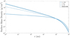 |
Fig. 1 Initial surface mass densities of Disc 5 for WD discs with λ = 1.6, 3, and 17 (solid, dashed, and dash-dotted, respectively) compared with that for the VE disc (dotted). More inefficient WD discs lead to flatter surface mass densities due to the stronger wind mass loss. All the discs have initially the same mass. |
2.1.3 Disc and stellar accretion
In Tabone et al. (2022), the local mass accretion rate varies across the disc due to the wind mass loss as
 (13)
(13)
where Ṁ* and ṀD are the stellar accretion rate and the disc accretion rate, respectively, and are defined at the inner wind launching radius rin and the outer wind launching radius rc, respectively, so that
 (14)
(14)
 (15)
(15)
The disc mass accretion rate is obtained as follows from Equation (C8) of Tabone et al. (2022):
 (16)
(16)
 (17)
(17)
We can use this expression of ṀD in Equation (13) to calculate the local mass accretion rate Ṁacc.
Alternatively, we can find the experssion of Ṁ* to calculate Ṁacc . The local mass accretion rate Ṁacc is related to the cumulative wind mass-loss rate Ṁw as
 (18)
(18)
Tabone et al. (2022) defines the mass ejection-to-accretion ratio as
 (19)
(19)
Using this definition and evaluating Equation (18) at r = rc, the stellar mass accretion rate is written as the disc mass flux ṀD reduced by the fraction mass that is effectively accreted onto the growing star:
 (20)
(20)
Figure 2 illustrates the radial dependence of Ṁacc normalised by ṀD for λ = 1.6,3, and 17 (black dashed, solid, and dotted lines, respectively). Also plotted are normalised ṀD (red line) and Ṁ* (blue lines). As expected from Equations (14) and (15), Ṁacc agrees with Ṁ* and ṀD at rin and rc, respectively.
The disc accretion rate of the VE disc is not explicitly shown, but corresponds to the red horizontal line in Figure 2, because the local disc accretion rate there is independent of the radius, and thus Ṁacc = Ṁ* = ṀD. For the WD discs, the local disc accretion rate has a radial dependence and the slope becomes steeper for a smaller λ due to a more substantial mass loss. Furthermore, since the value of ṀD is the same for all the cases, the stellar mass accretion rate decreases for the lower λ.
Next, we compare the evolution of the adopted disc models with the observed stellar mass accretion rates (Figure 3) and the observed distribution of the disc mass and the stellar mass accretion rate (Figure 4). Instead of randomly choosing disc parameters, we have selected nine disc models that have a combination of the initial disc masses of 0.2 M⊙, 0.06 M⊙, or 0.02 M⊙ and the total alpha parameters of αtotal = 7.4 × 10⁻², 7.4 × 10⁻³, or 7.4 × 10⁻⁴ (see Table 1). One of the reasons for this choice is that these are the same set of parameters used by Matsumura et al. (2021), so it makes the comparison easier. Another reason is that choosing a particular set of parameters rather than the random ones makes it easier to highlight the effects caused by a single parameter such as λ.
Figure 3 compares the stellar accretion rates Ṁ* as a function of time for Discs 1–9 that are calculated from Equation (20) with the observed stellar accretion rates for different ages that are shown in various symbols (see the caption for references). For all the disc models shown in solid lines, we have chosen αSS = 10−4 and λ = 3. For Discs 1-3, for example, αtotal = 7.4 × 10⁻² for all, and the initial disc masses are 0.2 M⊙, 0.06 M⊙, and 0.02 M⊙, respectively. For these discs, Disc 1 has the highest mass accretion rate while Disc 3 has the lowest, but the overall disc evolution timescales are similar and discs are gone within ~2 Myr. For Discs 4–6 and Discs 7–9, αtotal = 7.4 × 10⁻³ and 7.4 × 10⁻⁴, respectively. The trends for these groups of discs are similar to Discs 1–3, but the disc lifetimes become longer due to the smaller alpha values. Overall, although each of these disc models has a comparable Ṁ* to some of the observed systems, none of them produce the highest observed Ṁ* for different ages.
For Disc 5 (magenta line), we have also plotted the purely viscously evolving disc (dotted line) and the cases for λ = 1.6 (dashed line) and 17 (dash-dotted line) for comparison. As expected from Figure 2, the lower λ disc has the lower stellar accretion rate due to a more substantial mass loss. Since we don’t take account of the photoevaporation effect for the VE disc, it has a very long disc lifetime.
Figure 4 compares the MD – Ṁ* relation of WD and VE discs at 2 Myr for Discs 1–9 with the observed distributions of MD – Ṁ* in Lupus and Chamaeleon I star forming regions (shown in green and orange crosses, respectively, taken from Manara et al. 2019). An isochrone is drawn for the evolution of the same disc mass (and the same λ for WD discs) but with different αtotaı, which changes from 10−4 to 10−1 to encompass the range of αtotal for our disc models. We have also marked the cases with αtotal corresponding to Discs 1–9, with diamond symbols highlighting those capable of producing at least one giant planet with ≥30 M⊕ within 2 Myr. Discs 1–3 for WD discs are absent because these discs deplete by 2 Myr (MD < 10−4.5 M⊙), as seen in Figure 3. WD discs, with their rapid disc drainage capability, cover a broader range of low-disc-mass and low-stellar-accretion rate parameters compared to VE discs. The figure illustrates that the evolutionary paths of WD discs align reasonably well with the observational data with comparable ages. However, as in Figure 3, none of the disc models reproduce highest mass accretion rates over a range of disc masses.
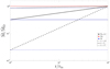 |
Fig. 2 Radial profiles of the local disc accretion rates Ṁacc normalised to the disc accretion rate ṀD are shown for Disc 5 with λ = 1.6 (black dashed line), λ = 3.0 (black solid line), and λ = 17 (black dotted line). Also plotted are the normalised stellar mass accretion rate Ṁ* (blue lines) and the normalised disc mass loss rates ṀD (red line). For the same disc model, ṀD is the same for all values of λ. Due to the substantial wind mass loss, the smaller λ leads to the steeper radial dependence of Ṁacc. |
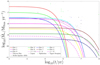 |
Fig. 3 Temporal profile of stellar accretion rates for the nine discs studied in this work (Table 1) when λ = 3. Additionally, cases with λ = 1.6, λ = 17, and purely viscously evolving scenarios for disc 5 are also shown. Various symbols correspond to observed values: black cross markers: Batalha & Basri (1993); Galli et al. (2015); Nuernberger et al. (1997); Andrews et al. (2018); Alcalá et al. (2014); Green cross markers: Andrews et al. (2018); Erickson et al. (2011); Andrews et al. (2010); Blue cross markers: Herczeg & Hillenbrand (2014); Garufi et al. (2020); Sicilia-Aguilar+2020: Sicilia-Aguilar et al. (2010). |
Initial disc mass MD,0 and the total value of the parameter αtotal of nine disc models.
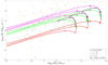 |
Fig. 4 Relation of MD − Ṁ* for the WD and VE discs at 2 Myr for Discs 1–9 compared with the corresponding distributions in Lupus (green) and Chamaeleon I (orange) star forming regions. The observational data are taken from Manara et al. (2019). The disc numbers with diamonds imply that the discs produced giant planets (≥30 M⊕) within 2 Myr. |
2.2 Planet formation via pebble accretion
2.2.1 Pebble accretion
Pebble accretion is a novel mechanism in the formation of planetary systems, which involves the gradual accumulation of centimetre to metre-sized particles called ‘pebbles’. We have estimated the pebble mass flux, ṀF, by using the ‘pebble formation front’ model proposed by Lambrechts & Johansen (2014). As dust particles aggregate and increase in size to form pebbles, they become highly susceptible to the influence of the headwind. This results in a pronounced inward migration of pebbles, supplying a substantial amount of solid mass to the inner regions of the disc. Generally, as the timescale for dust growth is longer at greater radii, the origin of the pebble mass flux, often referred to as the pebble formation front, progressively shifts outwards over time. We have computed the mass flux of pebbles swept by the pebble formation front by following Matsumura et al. (2021):
 (21)
(21)
where R0 and Rpeb represent the initial size of dust particles and the eventual size of pebbles at which they commence migration, respectively. For this work, we have chosen typical values of Rpeb ≈ 10 cm and R0 ≈ 1 µm. We replaced Ṁ* in Matsumura et al. (2021) with Ṁacc because the disc’s local accretion rate is no longer the same as Ṁ*. Σpg,0 is the initial pebble-to-gas surface mass density ratio and it is related to the stellar metallicity through
![${{{{\rm{\Sigma }}_{{\rm{pg}}}}} \over {{{\rm{\Sigma }}_{{\rm{pg}}, \odot }}}} \approx {10^{[{\rm{Fe}}/{\rm{H}}]}},$](/articles/aa/full_html/2025/01/aa52453-24/aa52453-24-eq25.png) (22)
(22)
where Σpg,⊙ = 0.01 is the value for the solar system. For our simulations, we have considered five different metallicities: [Fe/H] = (−0.5, −0.3,0,0.3,0.5)2. The timescale for the pebble formation front to reach the outer disc radius, tpf, is also calculated as in Matsumura et al. (2021) as
 (23)
(23)
Similar to Ṁacc, the mass flux ṀF is also a function of both time t and radial distance r. Since ṀF is proportional to Ṁacc, the pebble mass flux is higher in the outer disc.
Only a fraction of this pebble mass flux is accreted onto a protoplanet, and thus the pebble accretion rate can be expressed as follows by using the pebble accretion efficiency ϵ :
 (24)
(24)
We adopted the expression for pebble accretion efficiency ϵ as developed by Ida et al. (2016):
 (25)
(25)
where the efficiency is capped at unity and  with P being the pressure. The variables χ and ζ are functions of the Stokes number τs, and are defined as follows:
 (26)
(26)
 (27)
(27)
The pebble aspect ratio is represented by  and is the ratio of the pebble scale height hp to the radial distance r, where hp is approximated by
 (28)
(28)
The parameter  , related to the impact parameter b by
  , describes the interaction zone for a pebble approaching a protoplanet with mass Mp. The impact parameter b is estimated as,
 (29)
(29)
where the terms inside the minimum function refer to the Bondi and Hill accretion regimes, respectively. The Hill radius RH is given by  , and κ is the reduction factor for b when τs ≫ 1. The expression is derived by Ormel & Kobayashi (2012) as
 (30)
(30)
with  . Lastly, C, is given by
 (31)
(31)
which correspond to 2D and 3D accretion conditions, respectively.
2.2.2 Pebble isolation mass
Pebble isolation mass (PIM) is a critical mass in the growth of planetary cores. This stage is marked by a significant alteration in the gas surface density profile caused by the gravitational influence of the growing protoplanet. The alteration is such that it reverses the pressure gradient in the vicinity of the protoplanet. Consequently, instead of experiencing headwind that facilitates their inward drift, pebbles encounter a tailwind, effectively halting the flow of pebbles (e.g., Johansen & Lambrechts 2017; Ormel 2017). In this work, the PIM from Ataiee et al. (2018) is adopted as follows:
![$\matrix{ {{M_{{\rm{iso}}}} \approx \hat h_g^3\sqrt {37.3{\alpha _{{\rm{SS}}}} + 0.01} } \hfill \cr {\,\,\,\,\,\,\,\,\,\,\,\,\,\,\,\,\,\,\,\, \times \left[ {1 + 0.2{{\left( {{{\sqrt {{\alpha _{{\rm{SS}}}}} } \over {{{\hat h}_g}}}\sqrt {{1 \over {\tau _s^2}} + 4} } \right)}^{0.7}}} \right] \times {M_*}.} \hfill \cr } $](/articles/aa/full_html/2025/01/aa52453-24/aa52453-24-eq41.png) (32)
(32)
In Ataiee et al. (2018), it was found that protoplanets reaching PIM opens a gap and the surface mass density there decreases by up to 20%. On the other hand, Johansen et al. (2019) identified the gap transition mass that corresponds to a 50% gap, where migration switches from type I to type II:
 (33)
(33)
However, as indicated in Figure 3 in Matsumura et al. (2021), the planetary mass to reach a 50% gap becomes smaller than that to reach a 20% gap in the outer part of the disc, which is counterintuitive. Therefore, in our simulations, pebble accretion ceases once the planetary mass reaches min(Miso, Mtrans).
2.3 Gas envelope accretion
The critical core mass marks the point beyond which the hydrostatic equilibrium breaks down for the gas envelope, and thus the envelope contraction rather than the mass accretion is necessary to support the envelope (Ikoma et al. 2000). This envelope contraction leads to rapid gas accretion, and thus the critical core mass is often used as the starting point of gas accretion in planet formation models. We adopted a fitting formula of a critical core mass as a function of pebble accretion rate derived by Ogihara & Hori (2020):
 (34)
(34)
The above equation suggests that gas accretion commences when the mass accretion rate Ṁp becomes small enough, either due to the attainment of the PIM or the depletion of the pebble flux.
Once this condition is met, the gas accretion onto a protoplanet is constrained by both the rate at which a protoplanet can accumulate gas and the rate at which a disc can deliver gas to the protoplanet (Ida et al. 2018):
![${\dot M_p} \approx \min \left[ {{{\dot M}_{{\rm{KH}}}},{{\dot M}_{{\rm{acc}}}},{{\dot M}_{{\rm{TT}}16}}} \right].$](/articles/aa/full_html/2025/01/aa52453-24/aa52453-24-eq44.png) (35)
(35)
Initially, a protoplanet core accretes gas according to the Kelvin- Helmholtz contraction rate (Hori & Ikoma 2010):
 (36)
(36)
As the mass of the protoplanets’ gaseous envelope increases, the gas accretion rate is determined either by Ṁacc or by ṀTT16 = flocal Ṁacc (Tanigawa & Tanaka 2016), where flocal is the accretion efficiency defined as
 (37)
(37)
with K being the gap depth factor defined by Kanagawa et al. (2015) as
 (38)
(38)
When ṀTT16 < Ṁacc, a sufficient amount of gas is supplied to a protoplanet, and thus the gas accretion rate is regulated by how quickly the protoplanet can accrete gas. When ṀTT16 > Ṁacc, on the other hand, the gas accretion rate is determined by how quickly the disc can supply gas to the protoplanet.
2.4 Planet migration
When the masses of protoplanets are low, they cannot open up a gap and thus undergo type I migration with a timescale of τmigl. We adopted the equation from Ida et al. (2018):
 (39)
(39)
As shown by Kanagawa et al. (2018), the parameter c typically ranges between 1 and 3, aligning well with the isothermal formula for type I migration outlined by Tanaka et al. (2002). In this work, we adopt c = 2.
As the mass of the protoplanets continually increases, they can open a gap and the migration switches to type II migration. Kanagawa et al. (2018) proposed the timescale for type II migration is essentially the same as the type I migration timescale, but with the gas surface density reduced in the gap. The timescale for type II migration is expressed as,
 (40)
(40)
where migration switches from type I to type II when K = 1/0.04 (Johansen et al. 2019) or when the planetary mass corresponds to Equation (33).
2.5 Initial condition
In this study, nine disc models with different initial masses and αtotal values are tested around a Sun-like star, as summarised in Table 1 (also see Figure 3). Five metallicities, [Fe/H] = –0.5, –0.3, 0, 0.3, and 0.5 and three magnetic lever arms, λ = 1.6, 3, and 17, are considered for each disc. The disc 5 with λ = 3 and [Fe/H] = 0 is selected as the fiducial case.
In each disc, 40 non-interacting embryos are logarithmically spaced between 1 and 100 au to track planet formation across the disc. Although a characteristic mass of a planetesimal formed via streaming instability is about a Ceres mass (~1.6 × 10⁻⁴ M⊕, Johansen et al. 2015), we have chosen the initial mass of an embryo to be 0.01 M⊕ for simplicity. The choice of a constant initial embryo mass across the disc is rather arbitrary, but this assumption ensures that the initial core masses are the same not only at different disc radii but also for different disc models. Furthermore, by adopting the initial masses that are two orders of magnitude higher than a Ceres mass, we are implicitly assuming that a protoplanet grows upto the pebble onset mass via planetesimal–planetesimal collisions. Johansen & Lambrechts (2017) showed that the pebble accretion onset mass is ~10–3–10–2 M⊕ in 0.4–4 au, and reaches up to ~ 10–1 M⊕ in the outer disc region (40–100 au). Lau et al. (2022), on the other hand, studied the formation and growth of planetary cores in a pressure bump and found the onset mass for pebble accretion can be reduced to ~ 10–4 M⊕. In Section 4, we briefly discuss the effects of radially dependent initial core masses.
In all simulations, planet formation ceases either when all the gas is depleted or, for the particularly long-lived discs 7, 8, and 9, when the discs reach their artificially set lifetimes of 100 Myr3.
3 Results
3.1 Growth tracks of planets in wind-driven and viscously evolving discs
First, we will present the general planet formation outcomes for various wind efficiencies of WD discs as well as a VE disc. Figure 5 shows the growth tracks of the planets in Disc 5 with the solar metallicity [Fe/H]=0 for λ = 1.6 (upper left), λ = 3 (upper right), λ = 17 (lower left), and a VE disc (lower right). These figures illustrate the mass growth tracks of logarithmically- separated, 20 non-interacting embryos instead of the default 40 embryos for clarity. The colour gradient indicates the log10 of the time taken to reach a certain mass. Black hollow symbols represent the critical core masses of the planets where they start gas accretion, while black solid symbols show where Mcore = Menv, which approximately corresponds to the onset of rapid gas accretion (Pollack et al. 1996). For the WD cases, the hollow symbols usually correspond to PIMs, but there are also cases in which cores start gas accretion before reaching PIMs. The black dash- dotted lines denote a total mass of 30 M⊕. Planets above these lines are considered giant planets in this work. Planets that migrated to the inner edge of the disc (0.01 au) are assumed lost; however, their growth trajectories are still depicted in the figures for consistency.
The four cases shown in Figure 5 have the same initial disc mass and the same αtotal, but different stellar mass accretion rates due to various wind mass-loss rates (see magenta lines for Disc 5 in Figure 3). This leads to very different outcomes of planet formation.
First, the VE disc case has few surviving planets due to rapid type I migration, which agrees with the outcome of previous studies (e.g., Matsumura et al. 2017). This is primarily because the assumed αtotal = αSS = 7.3 × 10⁻³ is too high to allow the survival of planetary cores. One giant planet survived at ~2 au, but the initial core was located very far from the central star (~20 au), which also agrees with the trend observed by previous pebble accretion studies with a comparable disc’s viscosity (e.g., Bitsch et al. 2019).
The λ = 17 case has the lowest wind mass-loss rate and there is only a weak radial dependence of the mass accretion rate (see Figure 2). This case has the similar initial surface mass density profile to the VE disc (see Figure 1) as well as the comparable stellar mass accretion rate up to ∼10 Myr (see Figure 3). However, planet formation outcome of the λ = 17 disc is quite different from the VE disc, because the disc turbulence parameter is much smaller in the WD disc (αSS = 10–4). A smaller αSS leads to a thinner pebble layer (see Equation (28)), which accelerates the pebble accretion. Once the PIMs are reached, protoplanetary cores accrete gas rapidly and become giant planets. The migration appears to slow down as the rapid gas accretion occurs because type I migration becomes faster with mass while type II migration becomes slower (see Equations (39) and (40)).
As it can be seen from the number of lost cores, planet formation with λ = 17 is much faster than the other two λ cases, and only giant planets have survived. Among WD discs with different λ values, αtotal, αSS, and αDW are the same, and thus the pebble scale height hp, the pebble accretion efficiency ϵ, and the pebble isolation mass Miso are independent of λ. The difference in planet formation rates among WD discs arises from the difference in the pebble mass flux ṀF that is proportional to the local disc accretion rate Ṁacc (see Equation (21)). The discs with λ = 17 have the least wind mass-loss rate and thus have the highest local disc accretion rate.
For λ = 17, giant planets are formed out of cores that are initially at ∼7 au or beyond, and various types of giant planets (i.e., hot, warm, and cold Jupiters) are seen from ∼0.02 au to ∼30 au. However, giant planets with wide orbital radii (beyond a few tens of au) were not formed because pebble accretion is slow there for our initial core masses.
Here, we also have in-situ formation of hot Jupiters with semimajor axes ≲0.1 au as well as warm Jupiters with semimajor axes of ∼0.1–1 au. Such formation of giant planets near the central star might be limited due to the recycling of the planetary atmosphere, where the flow of gas from the disc injecting a higher entropy gas into the planetary atmosphere and slowing down the atmospheric cooling and further gas accretion (e.g., Ormel et al. 2015; Ali-Dib et al. 2020). Since we have not taken this effect into account, it is possible that we are overestimating the number of hot Jupiters. For warm Jupiters, however, Savignac & Lee (2024) recently showed that such a recycling effect is not very strong at 0.1 au and weaker outside it, making the in-situ formation of WJs and potentially some HJs plausible. Even when in-situ formation of hot Jupiters is not possible, a disc similar to this may still be able to form such planets. If multiple giant planets are formed beyond ∼1 au, they could experience dynamical instabilities (e.g., Chatterjee et al. 2008; Jurić & Tremaine 2008; Matsumura et al. 2010). When the pericentre of a planetary orbit becomes small enough, a hot Jupiter or a warm Jupiter can be formed via the tidal circularisation.
The λ = 3 case has the intermediate wind mass-loss rate and has resulted in formation of both low-mass and high-mass planets. This kind of mass distribution was not observed in Matsumura et al. (2021), where we assumed “two-alpha” disc models, because the local disc mass flux was constant in radii. Some cores are lost to the central star due to rapid type I migration, but all planets formed from cores that are initially beyond ∼1.5 au survived. There is also a general mass gradient inside out. The surviving low-mass planets have small-orbital radii of <0.1 au while the surviving giant planets have orbital radii ranging from ∼0.1 au to several tens of au. These giant planets are formed from cores with initial radii of ≳5 au, and their masses peak for cores with initial radii of ∼20–30 au. A disc such as this may lead to formation of either a warm Jupiter with a low-mass inner companion or a short-period super Earth accompanied by a cold Jupiter.
The λ = 1.6 case has the largest wind mass-loss rate and thus has the steepest radial dependence of the disc mass accretion rate (see Figure 2). Thus, the dust mass flux also sharply decreases towards the central star and planet formation is slow. As a result, the disc only formed low-mass planets that did not reach PIMs.
These three types of planet formation trends are not unique to each λ. As seen in Figure 6, all types of planet formation (i.e., only low-mass, both low- and high-mass, and only high-mass planets) arise for appropriate combinations of the mass, lifetime, and metallicity of a disc for each λ. However, as we discuss in Section 3.2, a difference in λ does result in a difference in the overall planetary mass distribution of a system.
Figure 6 shows similar planet formation outcomes for Discs 1–9 with [Fe/H]=0 and λ = 3. Here, the initial disc mass decreases from left to right (i.e., 0.2 M⊙, 0.06 M⊙, and 0.02 M⊙) while the disc’s lifetime increases from top to bottom (i.e., αtotal = 7.4 × 10⁻², 7.4 × 10⁻³, and 7.4 × 10⁻⁴). Overall, when disc’s masses are low or lifetimes are short (e.g., upper-right panels, Discs 2, 3, and 6), planet formation is inefficient and only low-mass planets form. For higher (lower) λ values, the overall trends are similar, but planet formation is faster (slower), and thus more (less) massive planets are formed closer in (further out).
On the other hand, when disc’s masses are high or lifetimes are long (e.g., lower-left panels, Discs 4, 7, and 8 4), planet formation is efficient and giant planets are formed across the entire disc. For higher (lower) λ values, the overall trends are similar again, but more (less) cores are lost to the central star without becoming giant planets.
Finally, for intermediate cases (e.g., Discs 1 and 5), we have found that both low-mass and high-mass planets can be formed in the same disc. A system with such a jump in the mass distribution is characterised by two conditions: low-mass planets survive in the inner disc, and giant planets form further out. For both of these conditions to meet, we have found that the giant planet formation timescale needs to be roughly comparable to the disc accretion timescale (tPF ~ tacc,0), where the giant planet formation timescale measures the onset of rapid gas accretion (Mcore ~ Menv). Satisfying the first condition becomes somewhat easier in low λ discs (e.g., λ = 1.6), because the core survival rate becomes higher partly because it takes longer for inner cores (≲2 au) to reach the PIM and partly because type I migration slows due to the reduced surface mass density with a flatter profile.
For higher (lower) λ values, the overall trends are similar, though these intermediate cases with a mass jump happen for different disc numbers. More specifically, the mass jump tends to happen for lower (higher) disc masses with longer (shorter) disc lifetimes to satisfy tPF ~ tacc,0. Moreover, the mass difference between low- and high-mass planets for a higher λ case is smaller than that for a lower λ case.
Since the radial dependence of Ṁacc is steeper for a lower λ disc, and since ṀF is assumed to be proportional to Ṁacc, we may naively expect a steeper r dependence in planetary masses as well. However, the final core mass is set by the PIM that is independent of λ. Therefore, if there is a sufficient pebble mass flux for a long enough period of time, it is possible that we don’t find a strong dependence of planet formation outcomes on λ. Our simulations, however, show that this is not the case and we indeed see the effects of λ on planetary masses. We will discuss the dependence of planetary mass diversity on the magnetic lever arm λ in the next subsection.
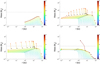 |
Fig. 5 Growth tracks of Disc 5 with [Fe/H]=0. Top left, top right, bottom left, and bottom right panels correspond to WD discs with λ = 1.6, 3, 17, and VE disc, respectively. Black open diamonds represent the core masses of the planets, while black solid diamonds show where Mcore = Menv. The black dash-dotted lines denote a total mass of 30 M⊕. |
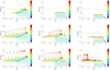 |
Fig. 6 Outcomes and evolution trajectories of single-core planet formation in nine wind-driven discs with the solar metallicity [Fe/H]=0, λ = 3. The first row, from left to right, corresponds to discs 1–3; the second row represents discs 4–6; and the third row denotes discs 7–9. |
3.2 How λ values affect the mass diversity in planetary systems
In this subsection, we will explore the effects of λ on the similarity or diversity of mass distributions. Figure 7 depicts the mass relationship between pairs of neighbouring planets for [Fe/H] = 0, with the outer planet’s mass plotted against that of the inner planet. The top left panel illustrates the scenario for λ = 1.6, the top right panel for λ = 3, the bottom left for λ = 17, and the bottom right panel displays the observed planetary systems around single FGK stars with stellar masses ranging from 0.45 to 1.4 solar masses. We have selected the data from the NASA Exoplanet Archive from September 2024 for planets with mass uncertainties below 30% (i.e., σM/M < 0.3). The colour of each marker represents the orbital period ratio between the outer and inner planets, while the unfilled circles in the bottom right panel are the observed pairs with ratios greater than 10.
To generate this figure, we have grown 40 non-interacting protoplanetary cores per disc that are initially logarithmically equally spaced between 1 au and 100 au. Pairs of neighbouring planets with final orbital radii greater than 0.01 au and less than 10 au were then selected. We have excluded pairs with the separation Km < 2, where  is defined as the orbital separation of two planets in terms of the mutual Hill radii
  . The critical Km value is motivated by the observed planet pairs, for which Km ranges from 2.32 to about 60 and peaks around 10–15. Furthermore, only planet pairs with an orbital period ratio Ti +1 /Ti ≤ 10 were considered5.
By eye, we can see that λ = 17 discs produce similarmass neighbouring planets within this period ratio range, while smaller λ discs such as λ = 1.6 produce a larger fraction of neighbouring pairs with vastly different masses. More specifically, the low λ discs form neighbouring planets with upto ~2 orders of magnitude mass difference not only when planets are widely separated Ti+1 / Ti ~ 10 but also when planets are closely separated Ti+1 /Ti ~ 2. On the other hand, although observed masses of neighbouring planets appear to be reasonably well-correlated, especially for lower-mass, closer pairs, there are also observed neighbouring planets with very different masses.
To statistically check for the peas-in-a-pod trend, many studies calculate the Pearson Correlation Coefficient (PCC). Although the PCC measures the strength of the linear relationship between two variables, it is not sensitive to the deviation from the 45-degree line, such as shifts in the distribution of points above and below the line or differences in slope. To quantify these effects, we have also calculated the Concordance Correlation Coefficient (CCC), which is the product of the PCC and the Bias Correlation Factor (BCF). The latter represents how closely the data points cluster around the 45-degree line. These values are also noted in each panel. For the lower-right panel, these values are shown for observed planet pairs with the period ratio Ti+1/ Ti ≤ 10, while the corresponding values for all observed planet pairs are shown in parentheses.
Observational data reveal a correlation between neighbouring planetary masses, with the PCC value of 0.73 and the corresponding p-value of p < 10–10. Otegi et al. (2022) studied peas-in-a-pod trends in radii, masses, densities, and period ratios for planets with <120 M⊕ and found a clear correlation for mass with the PCC value of ~0.5 and the p-value of 6 × 10⁻⁴. Mamonova et al. (2024) performed a similar study to Otegi et al. (2022), and found no mass correlation in their main sample, but found a weak correlation of 0.35 by excluding giant planets with masses above 100 M⊕. Rosenthal et al. (2024) found 0.476 for the mass correlation of giant planets. We have not found any increase in PCC values by excluding giant planets; the PCC value is 0.62 for <30 M⊕ and 0.76 for <100 M⊕. The decreased PCC value for <30 M⊕ compared to the full sample appears to be due to the lack of a group of planet pairs where one planet has >30 M⊕ and the other has <30 M⊕.
On the other hand, the obtained CCC value of 0.71 for observed data indicates a poor correlation and a strong deviation from the diagonal line and thus a significant deviation from the peas-in-a-pod trend in neighbouring masses. The CCC values are 0.57 for <30 M⊕ and 0.73 for <100 M⊕, and thus again, our sample does not show a tighter correlation by excluding giant planets.
For WD discs with all λ values, the PCCs are approximately 1 and corresponding p values are p ~ 10−50−10−100, which implies that all WD models studied here show significant correlation in the mass of planet pairs. On the other hands, the CCCs are 0.88, 0.96, and 0.98 for λ = 1.6, 3, and 17, respectively. The relatively low CCC (<0.90) for the λ = 1.6 disc indicates a poor correlation and a deviation from a similar-mass trend of neighbouring planets. For simulated planets, the mass correlations do not improve by excluding giant planets, because all of our simulations show very tight mass correlations for giant planets as seen in Figure 7. Both PCCs and CCCs in fact decrease by excluding giant planets.
Furthermore, observed data with Ti +1 /Ti ≤ 10 show that 59% of planet pairs are above the diagonal line so that the outer planet is more massive than the inner one, while 41% of pairs show the opposite trend. As seen in Figure 7, for all of the WD cases, the outer planets tend to be more massive than the inner ones. The fractions of planet pairs above the diagonal line are 99%, 64%, and 65% for λ = 1.6, 3, and 17, respectively. The fractions for λ = 3 and 17 are reasonably close to that estimated for the observed systems, though the observed planet pairs appear to be more symmetrically distributed around the diagonal line. This lack of symmetry is largely due to the lack of planet-planet interactions in our simulations. For interacting planetary cores, the mass distributions become more symmetric around the diagonal line as seen in, for example, Figure 7 of Mishra et al. (2021).
We have also tested how PCCs and CCCs change depending on the maximum Ti+1 / Ti. For observed data, we find that CCCs never become ≥0.90 even when we change the maximum Ti +1 /Ti ≤ so that neighbouring planetary masses are uncorrelated. For simulated planets, even for λ = 1.6, CCCs become ≥0.90 for Ti+1 /Ti ≤ 6, so neighbouring planetary masses are generally well-correlated except for relatively widely separated pairs. Furthermore, by testing other λ values, we have found that the CCCs become > 0.90 for λ ~ 1.8.
In summary, although we find that high λ discs tend to produce similar-mass planet systems while low λ discs can form more diverse-mass systems, a statistically significant mass diversity is observed only for low λ ≲ 2 and for relatively widely-separated planet pairs.
Finally, for lower and higher metallicity cases, the general trends of these distributions stay the same; the deviation from the diagonal line becomes stronger for smaller λ. However, for the lowest metallicity of [Fe/H] = −0.5, planet formation is less efficient and intermediate-mass planets with masses 10–100 M⊕ are scarce. For [Fe/H] = −0.5, none of λ cases lead to formation of diverse-mass planetary systems.
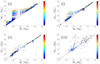 |
Fig. 7 Figure of Mp,out against Mp,in formed in wind-driven discs with [Fe/H] = 0 and different λ values. Top left: λ = 1.6. Top right: λ = 3. Lower left: λ = 17. Lower right: observation. |
3.3 The occurrence rate of CJs in SE systems
Bryan & Lee (2024) calculated the frequency of outer giant planets in SE systems, and found that the frequency is  for metal-rich stars ([Fe/H] > 0) and
  for metal-poor stars ([Fe/H] ≤ 0). Here, following Bryan & Lee (2024), we have estimated the occurrence rate of SE–CJ systems by calculating the frequencies of CJs with masses of 0.5–20 MJ and orbital radii of 1–10 au in systems with a SE with mass of 1–20 M⊕ and orbital radius of <1 au.
Figure 8 shows the occurrence rates of CJs in SE systems for various λ–[Fe/H] combinations. Since we have only focused on partiular disc masses and disc dissipation rates (represented by αtotal), the actual occurrence rates of SE–CJ systems could be overestimated or underestimated per λ–[Fe/H] combination. However, we still observed two general trends. First, there is a clear preference of SE systems that are accompanied by CJs in metal-rich discs ([Fe/H] ≥ 0). This is because only massive and/or long-lived discs tend to generate giant planets in metal-poor discs, and thus it is difficult to have SE-CJ systems. Second, there is also a clear preference of SE-CJ systems in low λ discs; specifically, the average occurrence rates for metal-rich discs ([Fe/H] ≥ 0) are 62%, 32%, and 23%, for λ = 1.6, 3, and 17, respectively. The high occurrence rate of SE–CJ systems in λ = 1.6 discs is caused by cores initially located beyond several au, which can reach the PIM fast enough in a high-metallicity environment to form CJs, whereas these cores did not grow into CJs in lower-metallicity environments. Since the occurrence rates of CJs in SE systems for λ = 1.6 and 3 are higher than the estimated value by Bryan & Lee (2024), metal-rich discs with λ ≲ 3 are expected to be good environments to generate SE-CJ systems.
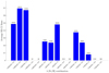 |
Fig. 8 Occurrence rates of CJs in SE systems for various λ-[Fe/H] combinations. The fractions of SE–CJ pairs out of SE systems with outer companions are shown above the histograms as well. The SE-CJ systems prefer high-metallicity discs ([Fe/H] ≥ 0) and/or low λ discs. |
3.4 How λ values affect planetary migration
Here, we will discuss how λ values affect planet migration. Figure 9 shows the extent of planet migration by semimajor axis ratios for both type I (solid curves) and type II (dashed curves) migrations.
For type I migration, we have plotted the migration extent for cores that never became giant planets and for those becoming giants. For the former, the ratios of the initial to the final semimajor axes are used, while for the latter, the ratios of their initial location to the location rcrit where they started rapid gas accretion (i.e., where Mcore = Menv) are chosen. If a core is lost to the star, its final location is assumed to be at the disc’s inner edge, 0.01 au, which results in step-like increments in the shaded region. The median semimajor axis ratios are approximately 7, 2.5, and 1.2 for λ = 17, 3, and 1.6, respectively. Thus, the figure shows that type I migration is less efficient in a lower λ disc. This is partly because planet migration itself slows down in a flat surface mass density disc (Ogihara et al. 2018), and partly because planet formation is slower in such a disc due to the lower mass flux.
These points can be seen in two extremes of the distributions as well. On one end, the shaded region represents the cores lost to the central star. The fractions of lost planets are approximately 5%, 25%, and 40%, for λ = 1.6, 3, and 17, respectively. So fewer cores were lost in low λ discs compared to high λ ones. On the other end, a large fraction of planets with the semimajor axis ratio near 1 arises from planets that barely grew. Since the fraction is the largest for λ = 1.6 and the smallest for λ = 17, the figure further confirms that planet formation is slower in the lower-λ discs.
Interestingly, despite that the planet loss rate is high (~40%) and comparable to that of the λ = 17 case, VE discs also have a large fraction of non-migrating planets (~30%), which is higher than the values for λ = 17 and λ = 3 (~10% and ~20%, respectively) though is not as high as λ = 1.6 (~40%). This is because planet formation is in fact slow in VE discs because the pebble scale height is larger compared to WD discs due to the higher disc’s viscosity. The large fraction of non-migrating planets arises mostly from the outer disc where formation timescales are long. On the other hand, VE discs also lose many planetary cores to the central stars because the PIM is higher due to the higher viscosity, and thus cores migrate further towards the star before reaching the PIM, accreting gas, and switching to slower type II migration. As it can be seen from Equation (40), since type I migration becomes faster as the mass increases while type II becomes slower, planet migration slows down once the gas accretion starts.
For type II migration, the semimajor axis ratio in Figure 9 represents the ratio of the critical radius for rapid gas accretion rcrit to the final location. Type II migration is also slower in WD discs compared to VE discs because αSS is smaller in WD discs. In other words, giant planets formed in VE discs migrate significantly after/during the gas accretion phase, while those formed in WD discs tend not to migrate much during this phase (typically less than a factor of two in terms of the semimajor axis ratio). Type II migration is also slower in lower λ discs compared to higher λ ones, partly because a flatter surface mass density profile leads to a smaller torque as in type I migration, and partly because giant planet formation takes longer in these discs, and thus a smaller amount of disc masses remain by that time.
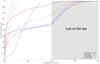 |
Fig. 9 Figure showing the ratios of the initial location to the critical location (rcrit) where giant planets started rapid gas accretion (solid lines), representing Type 1 migration. Dashed lines show the ratios of rcrit to the final location, representing Type 2 migration. Red, green, and magenta lines represent planets formed in wind-driven discs with λ = 1.6, 3, and 17, respectively, while blue lines represent those formed in purely viscously evolving discs. |
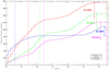 |
Fig. 10 Cumulative number of planets formed in wind-driven discs with λ = 1.6, 3, and 17, shown in red, green, and magenta lines, respectively. The blue line represents the planets formed in purely viscously evolving discs. The arrow lines and numbers represent the percentage of planets with a final mass greater than 30 M⊕, and the vertical dashed lines are the median values of planetary mass for each type of disc. |
3.5 How λ values affect the overall planetary mass
To show how λ values affect the overall final planetary mass distribution, we have plotted the cumulative mass distributions of surviving planets in Figure 10. Each coloured line includes 1800 single core formation simulations (9 discs × 40 cores × 5 metallicities). The arrows and numbers represent the percentage of surviving giant planets with a final mass greater than 30 M⊕, while the vertical dashed lines are the median values of planetary mass for each type of disc. The WD discs with λ = 1.6, 3, and 17 are shown in red, green, and magenta, respectively, while the VE discs are shown in blue.
The figure indicates that a larger number of planets survived in lower λ discs and that surviving planetary masses tend to be lower in such discs. These two outcomes are intertwined with each other. As described earlier, the discs with lower λ values are more efficient at preserving planets due to slower planet formation and migration, but this also means that the planetary masses tend to stay lower. For λ = 1.6, roughly 67% of surviving planets have <M⊕ and the median mass is ~0.3 M⊕, while for λ = 17, ~42% of surviving planets have <M⊕ and the median mass is ~3 M⊕. The difference in the numbers of surviving planets is in fact mainly caused by low-mass planets and the numbers of surviving giant planets are comparable to one another among WD discs (~400–500 out of 1800 cores).
Finally, although VE discs form the heaviest planets, the survival rate of giant planets and the median planetary mass are the lowest among all discs, owing to efficient migration and significant planet loss. This is primarily because the disc turbulence in VE discs is scaled with αtotal, which is higher than αss = 10−4 for WD discs.
3.6 How different metallicity values affect overall planetary mass and orbital radius
Here, we explore how metallicity affects planetary masses and orbital radii. Figure 11 shows the cumulative distributions of planetary masses (top panels) and their orbital radii (bottom panels) for low-mass (M < 30 M⊕, left panels) and high-mass (M > 30 M⊕, right panels) planets. These planets were formed in WD discs with λ = 3.
In order to quantitatively test the metallicity dependence, we performed the KS test on all cumulative distribution function (CDF) pairs shown in Figure 11. The results are summarised in Figures A.1 and A.2 for giant planets and low-mass planets, respectively. In each figure, the top-right triangle, composed of grids, represents the test results for orbital radius, while the bottom-left triangle represents the results for planetary mass. The two-sample KS statistic d and the corresponding probability p are shown for each metallicity sample pair. Grids representing orbital radius with p-values less than 0.05 are highlighted in red, while those showing planetary masses are highlighted in cyan.
Figure 11 shows that the mass distributions of low-mass planets (top left panel) vary depending on the metallicity, while those of high-mass planets (top right panel) are largely independent of the metallicity. This is confirmed by the KS tests. For low-mass planets, the null hypothesis is rejected for all pairs of metal- licities, suggesting that the disc metallicity significantly altered the mass distribution. Since the core accretion stage dominates the formation of such planets, higher metallicity leads to higher planetary mass. This trend, however, does not hold for giant planets. Although some metallicity combinations result in the p-value of <0.05, we cannot rule out the null hypothesis for the others. This is understandable because the PIM is independent of the metallicity (see Equation (32)) so gas accretion occurred on similar-mass cores. It should be noted that, although these curves appear similar, the number of planets included differs depending on metallicities. For the lowest metallicity environment, giant planet formation occurred only in relatively massive and long- lived discs (discs 4, 7, and 8), while for the highest metallicity environment, it happened in all the discs except for short-lived discs (discs 2 and 3). A kink seen for certain mass ranges in the distribution (e.g., 102.2 M⊕ ~ 103 M⊕) for [Fe/H] = −0.5 discs) arises due to rapid gas accretion so that few planets within that range of masses exist.
The bottom panels of Figure 11 show that the orbital radius distributions for low-mass and high-mass planets exhibit an opposite trend. For low-mass planets, higher metallicity environments lead to smaller orbital radii, while for high-mass planets, higher metallicity environments lead to larger orbital radii. Both of these are the results of more efficient planet formation in the higher metallicity environment.
For high-mass planets, the higher-metallicity environment leads to faster formation of cores, and thus gas accretion tends to be triggered at larger orbital radii. In fact, as seen from the bottom right panel, roughly 75% of giant planets in the higher metallicity environments (0.3 and 0.5) have cold Jupiters with orbital radii >1 au and nearly 40% of giants survived beyond 10 au. The lower-metallicity environment, on the other hand, results in slower formation and thus more migration of cores before triggering gas accretion. More than 40% of giant planets in the lowest-metallicity environment formed giants within 0.1 au.
For low-mass planets, on the other hand, the distributions are dominated by planets that were initially located in the outer part of the disc and thus were growing slowly. Indeed, more than 50% of the low-mass planets orbit beyond 10 au in the lowest metallicity environment, while this number decreases to 30% in the highest metallicity environment6.
The KS tests show that we can reject the null hypothesis for most cases of the radius distributions. Thus, our model predicts a metallicity gradient in the orbital distribution of gas giants in the quiescent environment where the gravitational perturbation effects were weak and the orbital distribution of giant planets just before the disc dissipation is well-preserved.
Finally, for lower and higher λ values, the overall trends are similar. For high-mass planets, both mass and orbital radius distributions for each metallicity have weak dependences on λ, and thus the distributions look very similar to Figure 11. For low- mass planets, masses tend to be lower and orbital radii tend to be larger for lower λ discs. This trend reflects the fact that planet formation is slower and migration is less efficient in lower λ discs.
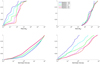 |
Fig. 11 Effects of metallicity on planetary masses and orbital radii for λ = 3. The top-left and top-right panels show the cumulative distribution of planetary mass for low-mass planets (M < 30 M⊕) and giant planets (M > 30 M⊕), respectively. The lower-left and lower-right panels display the corresponding cumulative distribution of their orbital radii. |
4 Discussion
In this section, we will discuss the effects of multiple-core formation and the radially dependent initial core masses.
4.1 Effects of multiple-core planet formation
Since the main purpose of our work is to investigate the effects of λ on formation and migration of planets, we have adopted a single-core planet formation model. However, multiple-core effects and their associated influences are likely important for planet formation in realistic protoplanetary discs.
In our model, all the planets are implicitly assumed to have nearly circular and coplanar orbits. The dynamical interactions among (proto-)planets can change eccentricities and inclinations of orbits significantly, which could affect both formation and the final orbital distribution of planets. For example, we adopt Equation (25) for the pebble accretion efficiency, but the formula does not take account of the effects of the randomness of orbits. For multiple-core simulations, it would be more appropriate to adopt an efficiency formula such as Ormel & Liu (2018) that includes the effects of eccentricities, inclinations, and disc turbulence. For zero eccentricity and inclination, these two efficiencies agree reasonably well with each other (Matsumura et al. 2021).
As the gas disc dissipates, the dynamical interactions among planets can lead to scattering, orbital crossing, and/or removal of some of the planets from the system, which drive eccentricities and inclinations of remaining planets (e.g., Chatterjee et al. 2008; Jurić & Tremaine 2008; Matsumura et al. 2010). When the eccentricity of a planetary orbit is high enough so that the pericentre of the orbit is close to the central star, the tidal interactions between the star and the planet can circularise its orbit, leading to formation of hot or warm Jupiters. Since higher metallicity discs tend to have a larger number of giant planets, such dynamical instabilities followed by the tidal circularisation of the orbit and the formation of a close-in planet may happen more frequently in a higher metallicity environment. Therefore, the orbital distribution trend seen in Figure 11 is likely to change when considering multiple-core planet formation. Furthermore, scattering among planetary cores is likely to transform the one-sided neighbouring mass distribution seen in Figure 7 into something more symmetric around the diagonal line, as seen in the observed systems.
Independent of the dynamical effects, the planet formation outcomes may also change when we consider the growth of multiple cores. Once a protoplanetary core reaches the PIM, it is expected to perturb the disc enough to create a pressure bump in the upstream that could trap the incoming flux of pebbles (e.g., Ormel 2017; Johansen & Lambrechts 2017). Such an effect can deprive protoplanets interior to the PIM core of the pebble flux and potentially create the dichotomy in the planetary system (Morbidelli et al. 2015). Our simulations have not taken this effect into account. However, in our simulations, there were no surviving cores inside the first surviving planet that reached the PIM. Therefore, we don’t expect a large difference in planet formation outcomes for inner protoplanets, even when we take this effect into account. The PIM core may also influence the growth of outer protoplanets. A recent work by Lau et al. (2024) has shown that the second generation of planets can be formed in a pressure bump due to the pebble accumulation there.
4.2 Effects of initial core masses
In this work, we have assumed constant initial core masses across the disc for simplicity. However, it is possible that initial core masses are radially dependent. We have tested two types of radially dependent initial embryo masses: those determined by the streaming instability (Liu et al. 2020) and those equal to the pebble accretion onset masses (Ormel 2017).
For the former, the streaming instability simulations predict that the most massive core masses are given by
 (41)
(41)
Where  is the relative strength between selfgravity and tidal shear,
  is the gas volume density. Since the core mass depends on the surface mass density and thus λ, the initial core mass varies not only radially but also for different disc models. A typical range of core masses is ~10−7 − 10−4 M⊕ at ~1 au, and it reaches up to ~10−2 − 10−1 M⊕ at ~ 100 au.
For the latter, the pebble accretion onset mass is given by
 (42)
(42)
This core mass also varies both radially and for different disc models via η and τs. A typical range of core masses is ~ 10−4 M⊕ at ~1 au, and it reaches up to ~10−1 M⊕ at ~100 au.
For both types of initial core masses, the main findings of this work remain largely unchanged. For λ = 1.6 with the SI- induced initial core masses, however, discs produce less SEs in the inner disc because planet formation is very slow due to very low embryo masses (down to ~10−7 M⊕). Nevertheless, λ = 1.6 discs still yield planetary systems with the greatest mass disparity among planets. Another difference is that giant planets are formed more efficiently in the outer disc, beyond a few tens of au, since initial core masses tend to be higher there in both cases.
5 Summary
In this paper, we have studied single-core planet formation in WD accretion discs via pebble accretion and explored the effect of the magnetic lever arm parameter λ on the outcome of planet formation and migration. We adopted the pebble accretion model developed by Ida et al. (2016) and a hybrid WD and VE disc model by Tabone et al. (2022).
A lower value of λ corresponds to a disc with a higher mass ejection rate, which results in a steeper radial dependence of the disc mass accretion rate, a lower stellar mass accretion rate, and a flatter surface mass density profile (Tabone et al. 2022). Overall, there are three main differences in formation and evolution of planets in different λ discs. First, planet formation is slower in lower λ discs compared to higher λ ones. This is because the disc mass dissipates faster and the pebble mass flux becomes lower in a lower λ disc.
Second, both type I and type II migrations are slower in a lower λ disc (see Figure 9 and Section 3.4). In such a disc, type I migration is slowed largely because of a flatter surface mass density profile, as proposed by Ogihara et al. (2018). Moreover, since type I migration becomes faster with planetary mass (see Equation (39)), less efficient planet growth in a lower λ disc leads to less migration overall. By adopting a new migration formula by Kanagawa et al. (2018), type II migration scales with type I migration, as can be seen in Equation (40), and thus a flatter surface mass density also leads to slower type II migration.
Third, a higher value of λ leads to a system of similar-mass planets, while a lower value of λ leads to a greater variety of planetary masses across the disc (see Figure 7). More specifically, although a planetary system with a mass jump can be found for all λ cases as long as tPF ~ tacc,0 (see Section 3.1), the mass jump tends to be larger for lower λ discs. We also found that the frequencies of SE-CJ systems are higher in lower λ and/or higher metallicity discs (see Section 3.2). The latter agrees with the observed preference of such systems around metal-rich stars (Bryan & Lee 2024). Combining the preference for similar-mass neighbouring planets and efficient migration in high λ discs, it is expected that such discs tend to lead to the formation of close-in, peas-in-a-pod, multiple-planet systems. From the discussions in Sections 3.2 and 3.3, we find that similar-mass and diverse-mass planetary systems are approximately separated at λ ~ 2–3.
Furthermore, our simulations also indicate the following effects of the stellar metallicity on formation and migration of planets. First, a higher-metallicity disc leads to a more massive and closer-in rocky planet compared to a lower-metallicity disc (see the left panels of Figure 11). This is because formation is faster, and thus a (proto-)planet has a longer time to migrate in the disc. Second, giant planet masses are expected to be largely independent of the metallicity (see the upper right panel of Figure 11) if the pebble isolation mass is independent of the metallicity, as assumed here. Third, if the dynamical evolution is quiescent, the metallicity gradient may be seen for orbital periods of giant planets. We expect giant planets in lower-metallicity discs tend to have shorter orbital periods compared to those in higher-metallicity discs (see the lower right panel of Figure 11) because the core formation takes longer in a lower metallicity disc, and thus cores migrate further before gas accretion.
Acknowledgements
We thank an anonymous referee for the prompt feedback. We thank Ramon Brasser, Man Hoi Lee, Tommy Chi Ho Lau, Shigeru Ida, and Aurora Sicilia-Aguilar for various discussions relevant to this work. SM would also like to thank the hospitality of the Konkoly Observatory, where part of this work was conducted.
Appendix A KS test results
The following two figures summarise the KS test results discussed in Section 3.6.
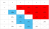 |
Fig. A.1 KS test results for metallicity analysis with λ = 3 for high-mass planets. The bottom-left triangle represents the test results for planetary mass, while the top-right triangle represents the results for orbital radius. The two-sample KS statistic d and the corresponding probability p are shown for each metallicity sample pair. Grids with p-values less than 0.05 for orbital radius are highlighted in red, and those for planetary masses are highlighted in cyan. |
References
- Alcalá, J. M., Natta, A., Manara, C. F., et al. 2014, A&A, 561, A2 [NASA ADS] [CrossRef] [EDP Sciences] [Google Scholar]
- Ali-Dib, M., Cumming, A., & Lin, D. N. C. 2020, MNRAS 494, 2440 [Google Scholar]
- Andrews, S. M., Wilner, D. J., Hughes, A. M., Qi, C., & Dullemond, C. P. 2010, ApJ 723, 1241 [Google Scholar]
- Andrews, S. M., Huang, J., Pérez, L. M., et al. 2018, ApJ, 869, L41 [NASA ADS] [CrossRef] [Google Scholar]
- Ataiee, S., Baruteau, C., Alibert, Y., & Benz, W. 2018, A&A 615, A110 [NASA ADS] [CrossRef] [EDP Sciences] [Google Scholar]
- Batalha, C. C., & Basri, G. 1993, ApJ 412, 363 [NASA ADS] [CrossRef] [Google Scholar]
- Birnstiel, T., Klahr, H., & Ercolano, B. 2012, A&A 539, A148 [NASA ADS] [CrossRef] [EDP Sciences] [Google Scholar]
- Bitsch, B., Izidoro, A., Johansen, A., et al. 2019, A&A, 623, A88 [NASA ADS] [CrossRef] [EDP Sciences] [Google Scholar]
- Blandford, R. D., & Payne, D. G. 1982, MNRAS 199, 883 [CrossRef] [Google Scholar]
- Bryan, M. L., & Lee, E. J. 2024, ApJ 968, L25 [NASA ADS] [CrossRef] [Google Scholar]
- Bryan, M. L., Knutson, H. A., Lee, E. J., et al. 2019, AJ, 157, 52 [Google Scholar]
- Chambers, J. 2019, ApJ 879, 98 [NASA ADS] [CrossRef] [Google Scholar]
- Chatterjee, S., Ford, E. B., Matsumura, S., & Rasio, F. A. 2008, ApJ 686, 580 [NASA ADS] [CrossRef] [Google Scholar]
- Emsenhuber, A., Mordasini, C., Burn, R., et al. 2021, A&A, 656, A69 [NASA ADS] [CrossRef] [EDP Sciences] [Google Scholar]
- Erickson, K. L., Wilking, B. A., Meyer, M. R., Robinson, J. G., & Stephenson, L. N. 2011, AJ 142, 140 [NASA ADS] [CrossRef] [Google Scholar]
- Ferreira, J., & Pelletier, G. 1995, A&A 295, 807 [NASA ADS] [Google Scholar]
- Galli, P. A. B., Bertout, C., Teixeira, R., & Ducourant, C. 2015, A&A 580, A26 [NASA ADS] [CrossRef] [EDP Sciences] [Google Scholar]
- Garufi, A., Avenhaus, H., Pérez, S., et al. 2020, A&A, 633, A82 [NASA ADS] [CrossRef] [EDP Sciences] [Google Scholar]
- Herczeg, G. J., & Hillenbrand, L. A. 2014, ApJ 786, 97 [Google Scholar]
- Hori, Y., & Ikoma, M. 2010, ApJ 714, 1343 [NASA ADS] [CrossRef] [Google Scholar]
- Huang, C., Wu, Y., & Triaud, A. H. M. J. 2016, ApJ 825, 98 [NASA ADS] [CrossRef] [Google Scholar]
- Ida, S., Guillot, T., & Morbidelli, A. 2016, A&A 591, A72 [NASA ADS] [CrossRef] [EDP Sciences] [Google Scholar]
- Ida, S., Tanaka, H., Johansen, A., Kanagawa, K. D., & Tanigawa, T. 2018, ApJ 864, 77 [NASA ADS] [CrossRef] [Google Scholar]
- Ikoma, M., Nakazawa, K., & Emori, H. 2000, ApJ 537, 1013 [NASA ADS] [CrossRef] [Google Scholar]
- Jiang, C.-F., Xie, J.-W., & Zhou, J.-L. 2020, AJ 160, 180 [NASA ADS] [CrossRef] [Google Scholar]
- Johansen, A., & Lambrechts, M. 2017, Annu. Rev. Earth Planet. Sci. 45, 359 [Google Scholar]
- Johansen, A., Mac Low, M.-M., Lacerda, P., & Bizzarro, M. 2015, Sci. Adv. 1, 1500109 [CrossRef] [Google Scholar]
- Johansen, A., Ida, S., & Brasser, R. 2019, A&A 622, A202 [NASA ADS] [CrossRef] [EDP Sciences] [Google Scholar]
- Jurić, M., & Tremaine, S. 2008, ApJ, 686, 603 [Google Scholar]
- Kanagawa, K. D., Tanaka, H., Muto, T., Tanigawa, T., & Takeuchi, T. 2015, MNRAS 448, 994 [NASA ADS] [CrossRef] [Google Scholar]
- Kanagawa, K. D., Tanaka, H., & Szuszkiewicz, E. 2018, ApJ 861, 140 [Google Scholar]
- Kokubo, E., & Ida, S. 2002, ApJ 581, 666 [Google Scholar]
- Lambrechts, M., & Johansen, A. 2014, A&A 572, A107 [NASA ADS] [CrossRef] [EDP Sciences] [Google Scholar]
- Lau, T. C. H., Dra?z?kowska, J., Stammler, S. M., Birnstiel, T., & Dullemond, C. P. 2022, A&A, 668, A170 [NASA ADS] [CrossRef] [EDP Sciences] [Google Scholar]
- Lau, T. C. H., Lee, M. H., Brasser, R., & Matsumura, S. 2024, A&A 683, A204 [NASA ADS] [CrossRef] [EDP Sciences] [Google Scholar]
- Liu, B., Lambrechts, M., Johansen, A., Pascucci, I., & Henning, T. 2020, A&A 638, A88 [EDP Sciences] [Google Scholar]
- Mamonova, E., Shan, Y., Hatalova, P., & Werner, S. C. 2024, A&A 685, A143 [NASA ADS] [CrossRef] [EDP Sciences] [Google Scholar]
- Manara, C. F., Mordasini, C., Testi, L., et al. 2019, A&A, 631, L2 [NASA ADS] [CrossRef] [EDP Sciences] [Google Scholar]
- Matsumura, S., Thommes, E. W., Chatterjee, S., & Rasio, F. A. 2010, ApJ 714, 194 [NASA ADS] [CrossRef] [Google Scholar]
- Matsumura, S., Brasser, R., & Ida, S. 2017, A&A 607, A67 [NASA ADS] [CrossRef] [EDP Sciences] [Google Scholar]
- Matsumura, S., Brasser, R., & Ida, S. 2021, A&A 650, A116 [NASA ADS] [CrossRef] [EDP Sciences] [Google Scholar]
- Millholland, S., Wang, S., & Laughlin, G. 2017, ApJ 849, L33 [NASA ADS] [CrossRef] [Google Scholar]
- Millholland, S. C., He, M. Y., & Zink, J. K. 2022, AJ 164, 72 [CrossRef] [Google Scholar]
- Mishra, L., Alibert, Y., Leleu, A., et al. 2021, A&A, 656, A74 [NASA ADS] [CrossRef] [EDP Sciences] [Google Scholar]
- Morbidelli, A., Lambrechts, M., Jacobson, S., & Bitsch, B. 2015, Icarus 258, 418 [NASA ADS] [CrossRef] [Google Scholar]
- Nazari, P., Tabone, B., Ahmadi, A., et al. 2024, A&A, 686, A201 [NASA ADS] [CrossRef] [EDP Sciences] [Google Scholar]
- Nuernberger, D., Chini, R., & Zinnecker, H. 1997, A&A 324, 1036 [NASA ADS] [Google Scholar]
- Ogihara, M., & Hori, Y. 2020, ApJ 892, 124 [Google Scholar]
- Ogihara, M., Kokubo, E., Suzuki, T. K., & Morbidelli, A. 2018, A&A 615, A63 [NASA ADS] [CrossRef] [EDP Sciences] [Google Scholar]
- Ormel, C. W. 2017, in Astrophysics and Space Science Library, 445, Formation, Evolution, and Dynamics of Young Solar Systems, eds. M. Pessah, & O. Gressel, 197 [NASA ADS] [CrossRef] [Google Scholar]
- Ormel, C. W., & Kobayashi, H. 2012, ApJ 747, 115 [NASA ADS] [CrossRef] [Google Scholar]
- Ormel, C. W., & Liu, B. 2018, A&A 615, A178 [NASA ADS] [CrossRef] [EDP Sciences] [Google Scholar]
- Ormel, C. W., Shi, J.-M., & Kuiper, R. 2015, MNRAS 447, 3512 [Google Scholar]
- Otegi, J. F., Helled, R., & Bouchy, F. 2022, A&A 658, A107 [NASA ADS] [CrossRef] [EDP Sciences] [Google Scholar]
- Pollack, J. B., Hubickyj, O., Bodenheimer, P., et al. 1996, Icarus, 124, 62 [NASA ADS] [CrossRef] [Google Scholar]
- Rosenthal, L. J., Howard, A. W., Knutson, H. A., & Fulton, B. J. 2024, ApJS 270, 1 [NASA ADS] [CrossRef] [Google Scholar]
- Savignac, V., & Lee, E. J. 2024, ApJ 973, 85 [NASA ADS] [CrossRef] [Google Scholar]
- Shakura, N. I., & Sunyaev, R. A. 1973, A&A 24, 337 [NASA ADS] [Google Scholar]
- Sicilia-Aguilar, A., Henning, T., & Hartmann, L. W. 2010, ApJ 710, 597 [Google Scholar]
- Steffen, J. H., Ragozzine, D., Fabrycky, D. C., et al. 2012, PNAS, 109, 7982 [NASA ADS] [CrossRef] [Google Scholar]
- Suzuki, T. K., Ogihara, M., Morbidelli, A., Crida, A., & Guillot, T. 2016, A&A 596, A74 [NASA ADS] [CrossRef] [EDP Sciences] [Google Scholar]
- Tabone, B. X. J. A., Cabrit, S., Des Forêts, G. P., et al. 2020, A&A, 640, A82 [CrossRef] [EDP Sciences] [Google Scholar]
- Tabone, B., Rosotti, G. P., Cridland, A. J., Armitage, P. J., & Lodato, G. 2022, MNRAS 512, 2290 [NASA ADS] [CrossRef] [Google Scholar]
- Tanaka, H., Takeuchi, T., & Ward, W. R. 2002, ApJ 565, 1257 [Google Scholar]
- Tanigawa, T., & Tanaka, H. 2016, ApJ 823, 48 [NASA ADS] [CrossRef] [Google Scholar]
- Weiss, L. M., Marcy, G. W., Petigura, E. A., et al. 2018, AJ, 155, 48 [Google Scholar]
- Zhu, W., & Wu, Y. 2018, AJ 156, 92 [Google Scholar]
Each of these terms corresponds to each term on the right-hand side of Equation (10) in Tabone et al. (2022), respectively.
In this work, we assume that the wind mass loss does not change the dust-to-gas ratio of the disc. If the wind mass loss increases the dust-to-gas ratio, the planets would grow in a more metal-rich environment, which could affect the formation outcome. We will leave this investigation for a future study.
This long disc lifetime does not affect the overall outcome of planet formation for most cases. For λ = 3, the exception is Disc 9 with [Fe/H] = 0 (see Figure 6) where some planets became giant planets within 20–30 Myr. Even later gas accretion was observed for λ = 1.6 with [Fe/H] = 0.5 and 0.3 in Disc 9 and with [Fe/H] = –0.3 in Disc 8, but we keep these results for the analysis because they don’t change the overall results.
Although an often adopted value is Ti+1 /Ti ≲ 4 (Weiss et al. 2018; Mishra et al. 2021), we have chosen a wider value because giant planets are often more widely separated (Ti+1 /Ti ~ 5–30, Rosenthal et al. 2024).
All Tables
Initial disc mass MD,0 and the total value of the parameter αtotal of nine disc models.
All Figures
|
Fig. 1 Initial surface mass densities of Disc 5 for WD discs with λ = 1.6, 3, and 17 (solid, dashed, and dash-dotted, respectively) compared with that for the VE disc (dotted). More inefficient WD discs lead to flatter surface mass densities due to the stronger wind mass loss. All the discs have initially the same mass. |
| In the text | |
|
Fig. 2 Radial profiles of the local disc accretion rates Ṁacc normalised to the disc accretion rate ṀD are shown for Disc 5 with λ = 1.6 (black dashed line), λ = 3.0 (black solid line), and λ = 17 (black dotted line). Also plotted are the normalised stellar mass accretion rate Ṁ* (blue lines) and the normalised disc mass loss rates ṀD (red line). For the same disc model, ṀD is the same for all values of λ. Due to the substantial wind mass loss, the smaller λ leads to the steeper radial dependence of Ṁacc. |
| In the text | |
|
Fig. 3 Temporal profile of stellar accretion rates for the nine discs studied in this work (Table 1) when λ = 3. Additionally, cases with λ = 1.6, λ = 17, and purely viscously evolving scenarios for disc 5 are also shown. Various symbols correspond to observed values: black cross markers: Batalha & Basri (1993); Galli et al. (2015); Nuernberger et al. (1997); Andrews et al. (2018); Alcalá et al. (2014); Green cross markers: Andrews et al. (2018); Erickson et al. (2011); Andrews et al. (2010); Blue cross markers: Herczeg & Hillenbrand (2014); Garufi et al. (2020); Sicilia-Aguilar+2020: Sicilia-Aguilar et al. (2010). |
| In the text | |
|
Fig. 4 Relation of MD − Ṁ* for the WD and VE discs at 2 Myr for Discs 1–9 compared with the corresponding distributions in Lupus (green) and Chamaeleon I (orange) star forming regions. The observational data are taken from Manara et al. (2019). The disc numbers with diamonds imply that the discs produced giant planets (≥30 M⊕) within 2 Myr. |
| In the text | |
|
Fig. 5 Growth tracks of Disc 5 with [Fe/H]=0. Top left, top right, bottom left, and bottom right panels correspond to WD discs with λ = 1.6, 3, 17, and VE disc, respectively. Black open diamonds represent the core masses of the planets, while black solid diamonds show where Mcore = Menv. The black dash-dotted lines denote a total mass of 30 M⊕. |
| In the text | |
|
Fig. 6 Outcomes and evolution trajectories of single-core planet formation in nine wind-driven discs with the solar metallicity [Fe/H]=0, λ = 3. The first row, from left to right, corresponds to discs 1–3; the second row represents discs 4–6; and the third row denotes discs 7–9. |
| In the text | |
|
Fig. 7 Figure of Mp,out against Mp,in formed in wind-driven discs with [Fe/H] = 0 and different λ values. Top left: λ = 1.6. Top right: λ = 3. Lower left: λ = 17. Lower right: observation. |
| In the text | |
|
Fig. 8 Occurrence rates of CJs in SE systems for various λ-[Fe/H] combinations. The fractions of SE–CJ pairs out of SE systems with outer companions are shown above the histograms as well. The SE-CJ systems prefer high-metallicity discs ([Fe/H] ≥ 0) and/or low λ discs. |
| In the text | |
|
Fig. 9 Figure showing the ratios of the initial location to the critical location (rcrit) where giant planets started rapid gas accretion (solid lines), representing Type 1 migration. Dashed lines show the ratios of rcrit to the final location, representing Type 2 migration. Red, green, and magenta lines represent planets formed in wind-driven discs with λ = 1.6, 3, and 17, respectively, while blue lines represent those formed in purely viscously evolving discs. |
| In the text | |
|
Fig. 10 Cumulative number of planets formed in wind-driven discs with λ = 1.6, 3, and 17, shown in red, green, and magenta lines, respectively. The blue line represents the planets formed in purely viscously evolving discs. The arrow lines and numbers represent the percentage of planets with a final mass greater than 30 M⊕, and the vertical dashed lines are the median values of planetary mass for each type of disc. |
| In the text | |
|
Fig. 11 Effects of metallicity on planetary masses and orbital radii for λ = 3. The top-left and top-right panels show the cumulative distribution of planetary mass for low-mass planets (M < 30 M⊕) and giant planets (M > 30 M⊕), respectively. The lower-left and lower-right panels display the corresponding cumulative distribution of their orbital radii. |
| In the text | |
|
Fig. A.1 KS test results for metallicity analysis with λ = 3 for high-mass planets. The bottom-left triangle represents the test results for planetary mass, while the top-right triangle represents the results for orbital radius. The two-sample KS statistic d and the corresponding probability p are shown for each metallicity sample pair. Grids with p-values less than 0.05 for orbital radius are highlighted in red, and those for planetary masses are highlighted in cyan. |
| In the text | |
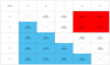 |
Fig. A.2 Similar to Fig. A.1 but showing the results of low-mass planets. |
| In the text | |
Current usage metrics show cumulative count of Article Views (full-text article views including HTML views, PDF and ePub downloads, according to the available data) and Abstracts Views on Vision4Press platform.
Data correspond to usage on the plateform after 2015. The current usage metrics is available 48-96 hours after online publication and is updated daily on week days.
Initial download of the metrics may take a while.