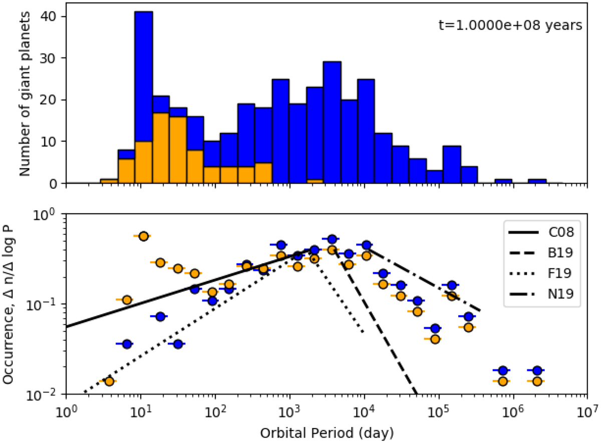
Top: distribution of orbital periods of giant planets at the end of the simulations (blue) and those of giant planets whose orbits are tidally evolved for 3 Gyr (orange, see Sect. 3.1.2). Bottom: corresponding occurrence rates of giant planets as a function of orbital period. The blue symbols only include simulated giant planets, while the orange ones include both simulated and tidally evolved giant planets. The rates are calculated for the number of planets per star per Δ log P = 0.23 to be compared with Fig. 3 of Winn (2018). The black slopes are occurrence rates estimated from observed planets. The solid, dashed, dotted, and dot-dashed lines correspond to d n∕d ln P ∝ P^{0.26 ± 0.1} for giant planets with >0.3 M_J within 2000 days from Cumming et al. (2008), for giant planets 5–5000 au from Baron et al. (2019), an asymmetric broken power law of d n∕d ln P ∝ P^{0.53 ± 0.09} and d n∕d ln P ∝ P^{−1.22 ± 0.47} with a break period of P_break = 1717 ± 432 days for giant planets with 0.1–20 M_J with periods ~1–10⁴ days from Fernandes et al. (2019), and dn∕d ln P ∝ P^−0.453 for giant planets with 5–13 M_J with periods ~1.16 × 10⁴−3.65 × 10⁵ days (~ 10–100 au) from Nielsen et al. (2019), respectively.