| Issue |
A&A
Volume 645, January 2021
|
|
|---|---|---|
| Article Number | A142 | |
| Number of page(s) | 24 | |
| Section | Interstellar and circumstellar matter | |
| DOI | https://doi.org/10.1051/0004-6361/201936043 | |
| Published online | 01 February 2021 | |
Continuity of accretion from clumps to Class 0 high-mass protostars in SDC335★
1
Jodrell Bank Centre for Astrophysics, Department of Physics and Astronomy, School of Natural Sciences, The University of Manchester,
Manchester,
M13 9PL, UK
e-mail: adam.avison@manchester.ac.uk
2
UK ALMA Regional Centre Node, Manchester, M13 9PL, UK
3
Intituto de Astrofísica de Andalucia (CSIC),
Glorieta de la Astronomia s/n, 18008,
Granada, Spain
4
School of Physics and Astronomy, Cardiff University, Queens Buildings, The Parade, Cardiff CF24 3AA, UK
5
Center for Astrophysics, Harvard & Smithsonian,
60 Garden St,
Cambridge,
MA 02138, USA
7
IAPS-INAF, Via Fosso del Cavaliere, 100,
00133 Rome, Italy
8
Max-Planck-Institut für extraterrestrische Physik,
Giessenbachstrasse 1,
85748 Garching, Germany
9
Max-Planck-Institut für Radioastronomie,
Auf dem Hügel 69,
53121
Bonn, Germany
10
Institut de Radioastronomie Millimetrique (IRAM),
300 rue de la Piscine,
38406 Saint Martin d’Hères, France
Received:
7
June
2019
Accepted:
17
November
2020
Context. The infrared dark cloud (IRDC) SDC335.579-0.292 (hereafter, SDC335) is a massive (~5000 M⊙) star-forming cloud which has been found to be globally collapsing towards one of the most massive star forming cores in the Galaxy, which is located at its centre. SDC335 is known to host three high-mass protostellar objects at early stages of their evolution and archival ALMA Cycle 0 data (at ~5′′ resolution) indicate the presence of at least one molecular outflow in the region detected in HNC. Observations of molecular outflows from massive protostellar objects allow us to estimate the accretion rates of the protostars as well as to assess the disruptive impact that stars have on their natal clouds during their formation.
Aims. The aim of this work is to identify and analyse the properties of the protostellar-driven molecular outflows within SDC335 and use these outflows to help refine the properties of the young massive protostars in this cloud.
Methods. We imaged the molecular outflows in SDC335 using new data from the Australia Telescope Compact Array of SiO and Class I CH3OH maser emission (at a resolution of ~3′′) alongside observations of four CO transitions made with the Atacama Pathfinder EXperiment and archival Atacama Large Millimeter/submillimeter Array (ALMA) CO, 13CO (~1′′), and HNC data. We introduced a generalised argument to constrain outflow inclination angles based on observed outflow properties. We then used the properties of each outflow to infer the accretion rates on the protostellar sources driving them. These accretion properties allowed us to deduce the evolutionary characteristics of the sources. Shock-tracing SiO emission and CH3OH Class I maser emission allowed us to locate regions of interaction between the outflows and material infalling to the central region via the filamentary arms of SDC335.
Results. We identify three molecular outflows in SDC335 – one associated with each of the known compact H II regions in the IRDC. These outflows have velocity ranges of ~10 km s−1 and temperatures of ~60 K. The two most massive sources (separated by ~9000 AU) have outflows with axes which are, in projection, perpendicular. A well-collimated jet-like structure with a velocity gradient of ~155 km s−1 pc−1 is detected in the lobes of one of the outflows. The outflow properties show that the SDC335 protostars are in the early stages (Class 0) of their evolution, with the potential to form stars in excess of 50 M⊙. The measured total accretion rate, inferred from the outflows, onto the protostars is 1.4(±0.1) × 10−3 M⊙ yr−1, which is comparable to the total mass infall rate toward the cloud centre on parsec scales of 2.5(±1.0) × 10−3 M⊙ yr−1, suggesting a near-continuous flow of material from cloud to core scales. Finally, we identify multiple regions where the outflows interact with the infalling material in the cloud’s six filamentary arms, creating shocked regions and pumping Class I methanol maser emission. These regions provide useful case studies for future investigations of the disruptive effect of young massive stars on their natal clouds.
Key words: stars: formation / ISM: jets and outflows / stars: massive / stars: protostars / ISM: clouds / masers
The reduced datacubes, images and spectra are only available at the CDS via anonymous ftp to cdsarc.u-strasbg.fr (130.79.128.5) or via http://cdsarc.u-strasbg.fr/viz-bin/cat/J/A+A/645/A142
© A. Avison et al. 2021
 Open Access article, published by EDP Sciences, under the terms of the Creative Commons Attribution License (https://creativecommons.org/licenses/by/4.0), which permits unrestricted use, distribution, and reproduction in any medium, provided the original work is properly cited.
1 Introduction
Molecular outflows are a commonly observed feature of the star-formation process detected toward protostars that will ultimately form stars covering a wide range of main sequence masses up to spectral type B (M* ~ 10M⊙) and beyond. The driving force responsible for such bipolar molecular outflows is thought to be the accretion of matter onto the central protostellar object from a disk coupled with the requirement for angular momentum to be conserved in the process (Konigl & Pudritz 2000; Pudritz et al. 2007; Tan et al. 2014; Rosen et al. 2020). The effects of limited resolution and obscuration impede the testing of theories of the exact physical mechanism driving these outflows observationally, be it X-wind or disk-wind driven (see e.g. Pudritz & Banerjee 2005; Pudritz et al. 2007; Frank et al. 2014), and the extent to which magnetic fields play arole. The breadth of the scales of molecular outflows, compared to the region from which they are driven, make them an invaluable tool when testing star formation theories. For example, they can be used to indirectly probe the accretion rates of material onto forming protostars (Bontemps et al. 1996; Duarte-Cabral et al. 2013).
In addition to providing information on the protostars that drive them, outflows also have an impact on their natal clouds by entraining matter as they inject energy and momentum into the surrounding interstellar medium (ISM) (Offner & Chaban 2017). This feedback may drive turbulence and ultimately help to disrupt the cloud. These effects have implications for the number and masses of stars (i.e. the initial mass function) which can form within a single molecular cloud (Duarte-Cabral et al. 2012; Plunkett et al. 2013; Krumholz et al. 2014; Zhang & Tan 2015; Drabek-Maunder et al. 2016). As a result, the observation of molecular outflows toward candidate high-mass protostars provides valuable information on the poorly constrained formation processes of such objects and their effects on the environments in which they form.
The infrared dark cloud (IRDC) SDC335.579-0.292 (hereafter, SDC335; Peretto & Fuller 2009) is an increasingly well-studied star-formingregion (Garay et al. 2002; Peretto et al. 2013; Avison et al. 2015) harbouring one of the most massive millimetre cores observed in the Milky Way. Seen in absorption against the mid-infrared background, SDC335 covers approximately 2.4 pc at its widest extent and displays six filamentary arms, which converge at the bright infrared source at its centre.
Using the Atacama Large Millimeter/submillimeter Array (ALMA) Cycle 0 data, Peretto et al. (2013) demonstrated that the whole SDC335 cloud is in the process of global collapse and that gas (traced by N2 H+) is flowing along the filamentary arms towards this central region. ALMA continuum data at 3 mm also highlighted two mm-cores, MM1 and MM2, with Mcore ~500 and 50 M⊙, respectively (Peretto et al. 2013). These data also included HNC observations indicating the presence of a molecular outflow from the MM1 core, however, that outflow has not been studied prior to this work.
Avison et al. (2015, hereafter, Paper I), used radio continuum data from the Australia Telescope Compact Array (ATCA) (from 6 to 25 GHz) to reveal that the MM1 core houses two Hyper Compact H II (HCH II) regions, whilst MM2 contains a single source, which also exhibits characteristics of an HCH II region. Each HCH II source was coincident with a Class II methanol (CH3 OH) maser, the pair of tracers clearly demonstrating SDC335 is in the process of forming three massive stars (each with M* > 9.0M⊙, based on their calculated Lyman α flux). Using this constraint on the upper end of the mass range in SDC335, the authors estimate a final stellar population in SDC335 of ~ 1400 (M* > 0.08M⊙, assuming a Kroupa 2002 IMF), suggesting that SDC335 could be a precursor to a massive cluster such as the Trapezium Cluster.
In this paper, we report on the molecular outflows observed in SDC335, which are likely to have been launched by the massive protostars therein. We present the observed molecular species and observations used to study the molecular outflows in SDC335 in Sect. 2. Section 3 describes the detected outflow properties and how they were measured. In Sect. 4, we discuss the measured properties and how this relates to the evolutionary status of the SDC335 high-mass protostellar objects. In Sect. 5, we discuss evidence for outflow-filament interactions. We present our conclusions and summarise our findings in Sect. 6.
2 Observations and ancillary data
Molecular line emission is key to understanding the morphologies and, more importantly, the kinematics and dynamic interactions of protostellar outflows. We present the results of SiO and Class I methanol (CH3 OH) maser observations made with ATCA toward SDC335 in combination with APEX1 and archival ALMA data, observing lines of CO, 13CO (ALMA only), and HNC (ALMA only), which allow us to study the outflows and their disruptive effects. Silicon monoxide, SiO, is depleted in the gas phase of the ISM (Walmsley et al. 1999), but it can be liberated from the grain mantels by shock fronts arising in molecular outflows (Schilke et al. 1997), making it a useful tool for studying outflows (e.g. Duarte-Cabral et al. 2014) particularly at outflow-cloud interaction points.
Similarly, the Class-I CH3OH maser (at 44 GHz) is regularly used as a tracer of outflows, (e.g. Cyganowski et al. 2009, 2011) as it is a collisionally excited maser species. Class-I CH3 OH masers are frequently seen as spatially offset from the local protostellar source, unlike the radiatively pumped Class-II CH3 OH maser species, lending support to the idea that the Class-I species is being excited in regions of interaction between outflowing material and the surrounding molecular material (Plambeck & Menten 1990; Kurtz et al. 2004; Voronkov et al. 2010). These lines and the observations characteristics are listed in Table 1.
Finally, CO, being ubiquitous in the ISM, provides sufficient molecular abundance to trace the high velocity gas entrained by the outflows. Thus, it is a good tracer of the large scale molecular outflow morphology, something that is not possible when observing shock-tracing species.
2.1 ATCA data
The ATCA data were taken in a single 12.5 h observing block on 3 September 2015 under the project code C3023. These observationscomprised two 2 GHz continuum bands within which four 64 MHz zoom bands were placed using the CABB correlator (Wilson et al. 2011). The primary target molecular lines used from these data are SiO (1–0) and the Class-I CH3 OH maser transition.
These observations were taken with ATCA in the ‘750B’ antenna configuration. During the data reduction, all baselines to the antenna at 6.0 km from the array centre were flagged out, meaning that these data have maximum and minimum baselines of 765.3 and 61.2 m, respectively. Data reduction was carried out in the software package MIRIAD using standard ATNF calibration and imaging strategies2. We note that poor atmospheric conditions at the start of observing meant that approximately four hours of data were entirely flagged from the start of the run, limiting the total observing time on source to ~ 4.7 h and setting the theoretical sensitivity to ~ 5.64 mJy beam−1 per 31.25 kHz channel.
2.2 ALMA Band 7 data
We use data taken from the ALMA archive, which forms part of the Cycle 1 observing program 2012.0.00781.S. For this work, we used the 12- and 7-m array observations at 330.64 and 345.874 GHz, which cover the 13CO(3–2) and CO(3–2) transitions, respectively.
These observations comprise a 39 pointing Nyquist sampled rectangular mosaic of the central region of SDC335, which is sufficient to cover the three HCH II regions observed in Paper I, with the 12-m array. This mosaic has a spatial extent of 65′′ × 68′′ centred at RA = 16h30m58.550s, Dec = −48°43′54.00′′. The 7-m data had a complementary 14 point mosaic pattern covering 74.6′′ × 69′′ centred at the same position, such that the whole 12-m mosaic region was covered (and fractionally exceeded). The data were downloaded from the archive, reprocessed, and the 12- and 7-m data were combined as per ALMA recommendations3 in the data reduction package CASA (McMullin et al. 2007), with a continuum subtraction applied.
For the 13CO data, the array was configured with minimum and maximum baselines of 10.7 and 1284.1 m, respectively4. During the CO observations the minimum and maximum baselines were 9.1 and 437.8m, respectively. The synthesised beam sizes of these data are given in Table 1.
Instrumental setup and image product properties used within this paper.
2.3 ALMA Band 3 data
ALMA Cycle 0 project 2011.0.00474.S was an 11 pointing mosaic observation at 90 GHz, covering the whole IRDC cloud seen in extinction against the mid-infrared background at 8 μm from Spitzer (seeFig. 1 and Fig. 1 of Peretto et al. 2013). The continuum and N2 H+ from these data were originally published in Peretto et al. (2013), though the line of interest in this current work, HNC, was not. The data were taken with 16 12-m antennas with no 7-m data taken (as this was not available with ALMA at the time). The array had maximum and minimum baselines of 18.3 and 197.7m.
2.4 APEX CO data
Single dish observations were made with the APEX telescope covering CO transitions (3–2), (4–3), (6–5) and (7–6). The observations of CO J = 4–3 (at 461.04077 GHz) and J = 3–2 (at 345.79599 GHz) were taken with the FLASH+ dual-channel receiver (Klein et al. 2014) on 3-4 June 2013. At the J = 3–2 transition the average system temperaturewas 300 K giving a typical root mean square(RMS) of 1.1 K in 0.1 km s−1 channels. For the J = 4–3 transition, the average system temperature was 1276 K, giving an average noise of 1.7 K in channels of a velocity width of 0.15 km s−1. The data was sampled on a 3′′ grid and then regridded during the data reduction to a resolution of 19.2′′ and 14.4′′ full width half maximum for the J = 3–2 and J = 4–3 observations, respectively. The emission at the (3–2) and (4–3) transitions shown in Fig. 2-D.
The CO transitions of J = 6–5 (at 691.473076 GHz) and J = 7–6 (at 806.651806 GHz) were observed simultaneously with the seven-pixel CHAMP+(Kasemann et al. 2006; Güsten et al. 2008) dual channel receiver on 30 May 2013. The (7–6) transition data were convolved to a grid with a 9.6′′ resolution during reduction to match the resolution of the (6–5) transition as shown in Fig. 2E. The RMS noise level across the maps was 1.2 K in 0.64 km s−1 channels and 2.2 K in 1.1 km s−1 channels for the lower and higher frequency transitions, respectively.
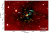 |
Fig. 1 Three colour image of SDC335 overlaid with ALMA CO contours highlighting three potential outflows within the cloud. Colour scale: Spitzer GLIMPSE three colour image with red, green and blue using 8.0, 4.5 and 3.6 μm respectively. Cyan and red contours: ALMA CO(3–2) integrated images showing the extent and morphology of the three potential outflows in the region with contours at ~ 9% to highlight their extent. The white ⋆ denote the locations of Class II CH3OH masers associated with the MM1a, MM1b and MM2 compact radio cores (Paper I). Orange dashed lines: nominal centroid positions of the six filaments seen in SDC335 (cf. Peretto et al. 2013). |
3 Outflow identification
To identify potential outflows within our data, a continuum subtracted data cube was created for each molecular line. These cubes have a velocity range from −100 to 0 km s−1 which is sufficient to cover the whole kinematic range of the observed species given the Vlsr of the target. The MM1 core has a Vlsr of −46.6 km s−1 and for MM2 Vlsr = −46.5 km s−1 (Peretto et al. 2013). The Vlsr of the compact radio cores observed by Paper I are consistent with those of the mm-cores based on their associated Class II (6.7-GHz) methanol masers, MM1a  = −48.0 to −45.0 km s−1, MM1b
  = −56.0 to −50.0 km s−1 and MM2
  = −51.0 to −43.0 km s−1 (Caswell et al. 2011), and the observed modulus offsets between molecular gas and peak maser emission of ~ 3 to 4 km s−1 (Szymczak et al. 2007; Pandian et al. 2009; Green & McClure-Griffiths 2011). As such, we adopted a Vlsr of −46.6 km s−1 for MM1a andMM1b and −46.5 km s−1 for MM2 in line with the mm-core values.
Using these cubes, the velocity ranges of each identified outflow for each molecular species were found by visual inspection and are listed in Table 2 (defined as the absolute offset from Vlsr to the last channel with a 3σ detection). Emission close to the Vlsr of the system is complex, particularly in the ALMA CO maps. As such, we implemented velocity range limits for our interpretation of the structures in SDC335. For all species, except CO, we excluded emission ±5 km s−1 from the Vlsr. For calculations of outflow properties with CO we use a larger velocity offset from the Vlsr as described in Sect. 3.2.4. The velocity ranges used for each outflow by species are given in Table 2. We then generated integrated intensity maps over these velocity ranges from which we measured the observed spatial extent and opening angles of each outflow wing.
Within the multiple datasets presented in this paper, there are three distinct molecular outflows observed within SDC335. We label these A, B, and C and we describe their respective morphologies, along with the identification of their likely progenitor protostars in Sect. 3.1. Figure 1 shows components of each outflow superimposed on a Spitzer IRAC three colour image of the SDC335 IRDC to highlight their spatial extent within the larger scale cloud. Figure 2 presents the morphology of each outflow as observed in CO, 13CO HNC (from ALMA), SiO (from ATCA), and CO from APEX. In Figs. 3–6, we present the spectra of each detected line from each outflow within the interferometric data. We also present spectra over the same velocity range as the outflows (−100 to 0 km s−1) at the peak position of each of the three HCH II at the CO, 13CO, HNC, and SiO tunings in Figs. A.1–A.3.
Velocity ranges used in calculating outflow properties and integrated intensity maps by observed species from ALMA and ATCA observed transitions.
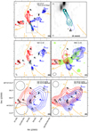 |
Fig. 2 Outflows in SDC335. Each panel includes the following data of the SDC335 region. Greyscale: 8 GHz continuum emission from Paper I. Orange dashed lines: filament centroids as per Fig. 1. Triangles: class-I CH3 OH maser positions (cf. Fig. 12 and Table 7). The ellipse in the bottom left of each plot and at top left in panels (A), (D) and (E) gives observed beam shape, which are the synthesised beam widths for interferometric and the HPBW for single dish observations, respectively. Beam shape values are given in Table 1. Each panel shows the integrated red- and blue-shifted emission from the detected outflows as red and blue contours, respectively over the velocity ranges listed in Table 2. Panel A: outflows in ALMA CO(3–2), as unfilled contours, and 13CO(3–2), as filled contours, the dashed box around outflow Ablue denotes the region shown in the adjacent panel. Panel A zoom: zoom in of region bordered by the dashed box in panel A, here the 13CO(3–2) emission isshown as the solid contour at the 10, 30, 45, 60, 75 and 90% of the peak integrated emission. The 10% contour of CO(3–2) is shown as the dotted contour for comparison to panel A. Panel B: ATCA SiO(1–0) emission. Panel C: ALMA HNC(1–0) emission, this panel also includes as the filled green contour the 4.5 μm emission above above 12.5 MJy sr−1 for the EGO observed in SDC335 (Cyganowski et al. 2009). (D) APEX detected CO(4–3), as solid contours, and CO(3–2), as dashed contours, emission at 50, 60, 70, 80 and 99% of the APEX data peak emission at each frequency. (E) APEX detected CO(6–5), as solid contours, and CO(7–6), as dashed contours, emission at 50, 60, 70, 80 and 99% of the APEX data peak emission at each frequency. Panels A and B: the contour levels are at 10, 30, 45, 60, 75 and 90% of the peak emission per outflow, panel C: the contour levels are at (5), 10, 20, 30, 40, 50, 70 and 90% of the peak emission per outflow (5% contour for red lobe only, to emphasise the curvature noted in the text). |
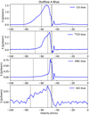 |
Fig. 3 Averaged spectra measured toward the blue lobe of outflow A for species CO, 13CO, HNC and SiO. The spectra are measured within the outer contour of the integrated intensity maps from Fig. 2 for each species. The vertical dashed line gives the Vlsr of the target and the vertical dotted lines mark the range in velocity from Table 2, based on which the integrated intensity maps were produced as were the CO outflow property calculations. The chosen limits are described in the main text. |
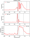 |
Fig. 4 Averaged spectra measured toward the red lobe of outflow A for species CO, HNC, and SiO. Measured and line markings as per Fig. 3. |
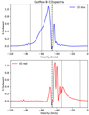 |
Fig. 5 Averaged spectra measured toward the blue and red lobes of outflow B for species CO. Measured and line markings as per Fig. 3. |
3.1 Outflow descriptions
3.1.1 A: north-south molecular outflow
The most apparent of the three outflows, namely, outflow A, runs approximately from north to south through the MM15 core. The outflow is detected in all tracers, SiO, HNC, CO (both ALMA and APEX), and 13CO (see Fig. 2). However, the red northern component of this outflow is not detected in the 13CO data. This is consistent with the trend seen throughout all the presented data, which shows that red-shifted emission is found to be weaker within each outflow. We attribute this to the geometry of the system, which is caused by the obscuring effect of self-absorption by the intervening material.
It is notimmediately clear to determine which of the two HCH II regions within MM1 is the progenitor of outflow A. As noted in Paper I, the area of maximal overlap between the two wings of the HNC outflow (Fig. 2, panel C) is coincident with the position of the MM1a compact radio source. At a higher resolution, the morphology of the red-shifted emission seems to show a slight curvature toward MM1b within the central core region, as seen in CO (3–2) and SiO (Figs. 2A and B), butthis could be due to interactions between the two outflows A and B (Sect. 3.1.3) originating from this region. Since the blue-shifted emission is elongated linearly with the major axis of emission aligned toward the MM1a core, we treat MM1a as the progenitor of this outflow. We measure an average length-to-width ratio for this outflow, at the 10% of peak integrated intensity contour in Fig. 2A, using both the red and blue lobes of 3.5.
3.1.2 Jet-like properties in outflow A
An inspection of the ALMA CO and 13CO data shows that the blue lobe of outflow A is highly collimated and exhibits a high velocity gradient. The length-to-width ratio of the ALMA CO and 13CO contour at the 10% of peak integrated intensity contours in Fig. 2Azoom are 2.8 and 3.4, respectively, matching the fiducial lower bounds of collimation of a jet structure (~ 3 e.g. Arcé et al. 2006)and comparable to other observed molecular jet sources, such as HH211 (Gueth & Guilloteau 1999) and Outflow C in IRAS 05358+3543 (Beuther et al. 2002). Figure 7 gives a position velocity (PV) diagram along the outflow axisas observed in CO outward from the driving source and covering a physical scale of ~ 0.09pc. We see that there is a clear linear velocity gradient within (highlighted by the white dashed line) from both CO emission (colour scale) and 13CO (displayed as a 5 and 10σ contours). From the CO data, we calculate a velocity gradient of 155 km s−1 pc−1. This value is comparable to molecular outflow velocities seen in other high mass sources, such as K3-50A (Klaassen et al. 2013).
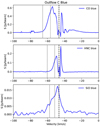 |
Fig. 6 Averaged spectra measured toward the blue (and only detected) lobe of outflow C for species CO, HNC, and SiO. Measured and line markings as per Fig. 3. |
3.1.3 B: east-west molecular outflow
Outflow B runs approximately east to west through the MM1 core and is seen primarily in the CO (both ALMA and APEX), with the redlobe seen in both HNC and SiO. The APEX CO data (at all four frequencies) is dominated by an EW component (Figs. 2D and E). The known extended green object (EGO) in SDC335 (Cyganowski et al. 2008)is orientated in this same east-west (EW) direction (green filled contour in Fig. 2C). The 4.5 μm emission responsible for EGO features is thought to be created predominantly by shocked H2 in outflowing material (Cyganowski et al. 2011, and references therein). Outflow B displays an average length-to-width ratio as measured inthe ALMA CO data of 3.0.
From the ALMA CO(3–2) data (Fig. 2A), the morphology of this outflow would suggest that MM1b is the likely progenitor. Interestingly it is approximately perpendicular, as projected on the sky, to the A outflow. This suggests, if MM1a and MM1b represent individual protostars, that their respective axes of rotation are likely to have very different orientations. Reasons for this misalignment in SDC335 are not clear from these data, but a possible scenario is considered in Sect. 5.3.
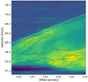 |
Fig. 7 Position velocity digram along the ABlue outflow axis. The PV data covers a physical size of 0.09 pc offset from the drivingsource (MM1a). Colourscale: ALMA CO(3–2) data. Contours: ALMA 13CO(3–2) data. The white dashed line shows the observed velocity gradient of ~155 km s−1 pc−1. |
3.1.4 C: NW (SE) molecular outflow
Outflow C is located to the north-west (NW) of the MM2 core. Detected in interferometric data in CO, HNC, and SiO, the molecular emission appears to be coming from a single outflow lobe, with its counterpart undetected, likely due to it having a similar velocity to the systemic velocity of SDC335 and, therefore, remaining in the excluded velocity range. This is supported by the presence of red-shifted emission in the APEX CO data that suggests the presence of a counterpart. This outflow hosts the brightest shock-tracing SiO emission of the three and the strongest Class-I CH3OH maser detected here. Due to the lack of a counterpart red lobe, we do not attempt to measure an average length-to-width ratio for this outflow.
3.1.5 Considering other possible outflows
The detection of the three outflows described above does not preclude the existence of additional outflows within SDC335. Using the ALMA band 7 CO data (the dataset with both the highest sensitivity and spatial resolution), we see that close to the Vlsr of the system, the potential for additional structures still remains. However, the current data in this region suffers from two issues arising frominterferometric artefacts: firstly, the bright CO emission and, therefore, the associated interferometric side-lobe artefacts are complex at these velocities; and secondly, owing to a lack of zero-spacing or single dish data, the ALMA image suffers from negative ‘bowling’ that comes from resolved-out extended emission in the source6, thereby further complicating the assessment of features at these velocities. These issues, combined with a lack of evidence for other outflows in our data at other frequencies, lead us to disregard some tentative structures which may appear to be additional outflows.
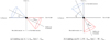 |
Fig. 8 Two limiting cases of the Cabrit & Bertout (1986) ‘case 2’ outflow morphology ascribed to outflows A and B. The Cabrit & Bertout (1986) ‘case 3’ outflow occurs when i is sufficiently large to make the rear of the blue lobe and front of the red lobe cross the dotted Vlsr line shown. |
3.2 Outflow properties
3.2.1 Inclination angles
To estimate the properties of the detected outflows, we must consider their inclination to the plane of the sky, measured as the angle i, with i = 0° indicating that the axis of the outflow is oriented along the observer’s line of sight and i = 90° indicating that it is perpendicular to the light of sight. To assess this, we used the ALMA CO integrated intensity maps (shown in Fig. 2A) as this dataset has the highest spatial resolution and signal-to-noise ratio. In the first instance, we assume each outflow has a symmetric biconical geometry, following Cabrit & Bertout (1986), and we define the opening angle, θmax, as the angle between the cone’s axis of symmetry and the outer emission contour at 3σ (see Fig. 8).
Next, we compare the measured θmax, the observed positions and morphology of the red and blue outflow lobes on the plane of the sky to the model outflows described by Cabrit & Bertout (1986). The work of Cabrit & Bertout (1986) includes four model ‘cases’ of differing inclination angle, i, and the opening angle (see their Table 1) to describe the morphology of the red and blue lobes an observer would expect to see on the sky for each given case. In brief7 the four cases are as follows:
Case 1 describes an outflow with both a red-shifted and a blue-shifted lobe on the line of sight, namely, with blue in front of a red lobe. The inclination angle conditions for this case are i < θmax and i ≤ 90° − θmax. Observationally, this yields an outflowing red-blue lobe pair, which overlap spatially on the line of sight.
Case 2 describes a case with two observed outflow lobes, again one red-shifted and one blue-shifted, but with the inclination angle conditions of this case as i ≥ θmax and i ≤ 90° − θmax (labelled A and B in Fig. 8). Observationally there will be no point in the plane of the sky where the red and blue lobes spatially (or kinematically) overlap.
Case 3 has outflow lobes which do not overlap spatially (as per case 2) but with the emission from each lobe in the pair spanning the source, Vlsr, resulting in mixed red-and-blue-shifted emission from each lobe. The Cabrit & Bertout (1986) model here requires inclination angles of values of i ≥ θmax and i > 90° − θmax.
Case 4 requires very large opening angle (θmax) and inclination angles which obey these conditions, i < θmax and i > 90° − θmax. This resultsin lobes that overlap spatially (as per Case 1) and also span the Vlsr and, as such, exhibit both red-shifted and blue-shifted emission (as per Case 3).
We notethat for the purposes of the current study, only cases 2 and 3 are relevant here. Outflow A has two spatially and kinematically non-overlapping lobes in the plane of the sky. This is indicative of a Cabrit & Bertout (1986) case 2 source. We find that the opening angle, θmax, of the blue-shifted part of outflow A is ~14°, putting loose limits on i of between 14 and 76°. Similarly, outflow B has two non-spatially or kinematically overlapping lobes, again indicating a Cabrit & Bertout (1986) case 2 source. We measure θmax as between ~9.4 and 12.6°, and use the average value of 11° in calculations giving i between 11 and 79°.
Determining the inclination of outflow C is complicated by the fact that only one lobe is reliably detected to the north-west of MM2. We could assume that C is a Cabrit & Bertout (1986) case 3 source (i ≥ θmax and i > 90°) given that the observed velocity range of the one observed lobe spans the Vlsr of MM2. This would give an inclination angle of >77° given our measured θmax of 13.4°. However, as the red lobe is not reliably detected in this source, we cannot confirm that the red lobe would similarly demonstrate an emission spanning the Vlsr and, therefore, we use, instead, the commonly adopted statistical average value of i = 57.3°. This average inclination angle, ⟨θ⟩ is calculated as:
 (1)
(1)
3.2.2 Further consideration of the outflow inclination angles for outflows A and B
Based solely on the Cabrit & Bertout (1986) models the potential inclination angles for outflows A and B cover ranges of 62° and 68°, respectively. Such broad ranges introduce significantly different correction factors when deriving outflow properties. These correction factors range between 1.0 and 5.2 to correct the measured length, velocity, and momentum, with between 1.0 and 27.5 for energy and 0.2 and 27.0 for momentum flux (see Sect. 3.2.4 for a description of these derived properties and their respective correction factors). To further limit the possible range of inclination angles, we now outline an additional consideration, beyond the Cabrit & Bertout (1986) models, based on the observed length-to-width ratios (LWRO) and the observed distance from the driving source to the maximum width (xO) of the observed outflows. We present in Appendix B the full geometric derivation of this morphology and our associated results.
Outflows A and B have observed length-to-width ratios of 3.5 and 3.0, respectively (average of both red and blue lobes for each). Given also these outflows’ observed opening angles, and assuming the biconical outflow morphology of Cabrit & Bertout (1986), we find that it is not possible to recover such observed length-to-width ratios with no external influence on the outflow. With their respective opening angles and a bicone morphology, the maximum recoverable LWRO for each outflow reaches an asymptote at angles of 76 and 79° and with values of LWRO of 2.1 and 2.6 for A and B, respectively. This is due to the fact that under the biconical outflow morphology the observed length, LO, is also the point along the outflow of maximum observed width.
In observations and modelling of molecular outflows, the idealised biconical morphology is seldom, if ever, seen (see e.g. Frank et al. 2014, and references therein). This is due to the influence of the environment on the outflow. In particular, modelling the effects of the collapsing clumps, precession, turbulence, and magnetic fields (see e.g. Rosen & Krumholz 2020) show that the outflow morphologies are narrower along the outflow axis than the bicone morphology would suggest. Given these effects and the fact that we cannot reproduce the observed LWR for outflows A and B using the biconical morphology, we instead propose an alternate morphology to limit the inclination angle ranges of these outflows.
Our proposed ‘pencil-like’ morphology allows the widest point can be at some arbitrary point, x, along the length (as is observed for outflows A and B). Using this second morphology (as detailed in Appendix B and Fig. B.1) we find inclination angle ranges of between 53 and 76° for outflow A and 59 and 79° for outflow B which can provide the observed LWRO.
An alternate scenario by which the observed LWRO for outflows A and B could be achieved would consist of observing these outflows at low inclination angles where the observed emission primarily arises from the outflow cavity rather than the outflow edge (i.e. Fig. 8a, as opposed to Fig. 8b or similar for our alternate morphology). In such a case, the observed length-to-width ratios would require shaping of the outflow cavity away from symmetry about the outflow direction by the surrounding medium, compressing and elongating the cross-section of the cavity in a single dimension. In the case of SDC335, to observe two outflows from driving sources separated by <9000 AU which display similar levels of compression of their outflow cavities but at orthogonal directions seems implausible.
We therefore consider it more likely that the outflows are inclined closer to the plane of the sky than along the line of sight. As such, we consider the lower bounds from the Cabrit & Bertout (1986) models as extreme values and base our analysis instead on values ranging from those allowed by the geometric arguments presented in Appendix B of 53 to 76° for outflow A and 59 to 79° for outflow B.
Table 3 provides the correction factors used for each outflow to correct the derived values to create the inclination angle corrected values given in Tables 4 and 5. For outflow C we use the correction factor at 57.3° and for outflows A and B we used average value of the correction function over the angle range given in Col. 3 of Table 4. For completeness, we also include in Table 3 the correction factors which would apply if the inclination angle ranges were based solely on the Cabrit & Bertout (1986) cases (given in italics) and in Appendix B, a brief discussion of the implications of using these correction factors.
The proper assignment of inclination angles to observed outflows is a difficult task and has significant implications on derived properties. With current leading observatories, for example, ALMA, providing a wealth of observed molecular outflows, it is timely for investigation to be set into a robust method of assigning these angles. We look forward to the possibility that the use of an alternate morphology in this work will raise further discussions of this matter.
Factors used corrected observed outflow properties to account for the inclination angle, i.
3.2.3 Temperature estimation
The four observed transitions of CO within the APEX data allow us to estimate the kinematic temperature of the outflowing gas in SDC335. To achieve this, we first regridded the data from each observation to the poorest spatial and velocity resolution, those being APEX CO (3–2) spatially and APEX CO (7–6) in velocity. We then created integrated intensity maps at 5 km s−1 intervals from each cube. For each observed outflow we measured the integrated intensity (in K km s−1) at two positions along the outflow, creating a spectral line energy distribution (SLED) at each position. We then followed the approach of Liu et al. (2018) by generating a large grid over temperature, number and column density with the radiative transfer code RADEX (van der Tak et al. 2007) and searching for the best-fit modelled intensities compared to our observed SLED intensities to give a temperature at a given position. The best fit being a χ2 ~ 1 following the χ2 approach of van der Tak et al. (2000). We then take all models with χ2 = 1 ± 0.05 and use the average properties of these models. Figure 9 gives an example of the APEX CO intensities and best fit model at a given position and velocity along outflow A. Using this technique we find Tkin values of 62/53 K, 54/61 K and 55 K for the blue and red components of outflows A, B and C respectively, (see Table 5).
Measured and derived outflow properties.
CO(3–2) outflow properties derived from ALMA data.
3.2.4 Derived properties
Using the inclination angles discussed in Sect. 3.2.2, we were able to calculate inclination corrected physical properties for each outflow. For each observed species, we provide in Table 4 both the measured and inclination angle corrected outflow lobe length, l and |Vmax|. We use the inclination-corrected values to calculate a dynamical time, tdyn, for each outflow lobe. We define these properties and their inclination angle correction factors following Cunningham et al. (2016, and references therein), as follows:
The lobe length, l, is the maximum distance from the progenitor peak to the 3σ emission contour over the wings velocity range. The corrected length is calculated as lcorr = lmeasured∕sin(i) for inclination angle i. The absolute velocity difference, |Vmax|, is defined as the difference between the outflow progenitor’s Vlsr and the final velocity channel in the image cube to show 3σ emission from the outflow, with a correction for i is calculatedas  . Finally, tdyn, the dynamical age of the outflow is calculated as
 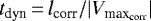 .
.
For the ALMA CO observations, we also provide in Table 5 the mass, momentum, and energy of each outflow lobe, following the methods of Duarte-Cabral et al. (2012). As part of this analysis, we note that, as may be expected for a high mass star forming molecular cloud, emission close to the systemic velocity of the cloud becomes increasingly complex, with features of self absorption and missing large scale flux in the interferometric data, which can lead to uncertainties in values derived from emission observed within these velocity ranges. In order to avoid basing our findings on velocity ranges within the data effected by self-absorption or imaging artefacts, we exclude data close to the systemic velocity in the following way.
For the MM1 core, we take the spectrum of CO (3–2) data from APEX over the whole SDC335 velocity range. We fit a Gaussian to this spectrum, centred at the Vlsr and exclude emission from channels ±2.5 × the variance, σ, of this Gaussian fit. The fitted σ was found to be 5.2 km s−1. The factor of 2.5 was chosen to ensure that all self-absorption and missing flux features in the interferometric data were excluded for the MM1 core outflows (A and B) as can be seen in Figs. 3–5. Excluding these velocity channels means our derived properties are lower limits for outflows A and B.
We repeat the same process for the MM2 core, taking the APEX CO (3–2) spectrum and fitting a Gaussian. Here, σ is found to be 6.7 km s−1. The velocity range of the observed outflow lobe C from source MM2 is very close to the Vlsr of MM2 that to exclude emission from ±2.5σ velocity channels would remove too much emission to provide a realistic determination of the values. Instead we use ± 1.5σ sufficient to avoid self absorption artefacts in the CO data and retain sufficient data to get a meaningful result. The velocity ranges used for calculating outflow properties and generating the integrated intensity images of each outflow lobe shown in Fig. 2 are given in Table 2.
Although we have other molecular species in the current data we do not carry out the following calculations with the data for these reasons. In particular, SiO is a shock-tracing species and therefore cannot reliably trace the bulk outflow properties since it will be enhanced in regions of shocks and less abundant elsewhere; HNC is currently a poorly studied outflow tracer therefore it is not clear whether or not (like CO) it traces the bulk outflow properties and further studies of this species in multiple targets would be required to assess its nature in outflows, which is beyond the scope of this paper.
For our calculations with the CO ALMA data, we define mass within the outflow, Mout in units of M⊙, as:
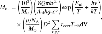 (2)
(2)
where μ is the mean molecular mass, NA the Avagadro’s constant, Q the partition function, and Aul the Einstein coefficient. Eul and gu are the energy of the transition in K and the statistical weight of the upper energy level (2J+1), respectively, and D is this distance to SDC335 (3.25 kpc). The value given by  is equivalentto the integrated intensity and is calculated from the data cubes within a polygon region around each lobe. The sum is made per pixel, x, y, per velocity channel, v, over the outflows respective velocity range for all pixels with an intensity greater than or equal to three times the RMS per channel. Within this sum the data units are converted from the native units Jy beam−1 to Kelvin. The factor τcorr gives the optical depth correction factor of the form
  and dV gives the channel velocity width in km s−1.
We calculate the mass both with a lower bound temperature T of 20 K and a literature value for τcorr of 3.5 (Cabrit & Bertout 1992) as well as the temperature values recovered from our best fit radiative transfer models from Sect. 3.2.3 (Table 5) with a τcorr factor of 8.2 based upon our estimated 12CO optical depth. To estimate an optical depth for 12CO in the outflows, we use the 13CO to 12CO line ratio observed in the blue wing of outflow A. Following the procedure of Myers et al. (1983), we compare the 13CO/12CO line ratios observed at multiple points (at peak emission) along the outflow to the ratio of optical depths given by  and use the assumption that
  is equal to
  . Here, f is the isotopic abundance ratio, in the range f = 50−100 typical of star-forming regions (e.g. Pineda et al. 2010; Szűcs et al. 2014). Given this range of f we can derive numerically a range of optical depths for 13CO and thus attain a corresponding range of
  values. We find a range of
  = 2.4 and 23.5 and use the median value of 8.2. These are comparable to typical values seen in CO outflows e.g. (Cabrit & Bertout 1992) of 1 to 8.9 with a median of 3.5.
Momentum and energy then follow as:
 (3)
(3)
where ΔV is the absolute velocity difference between the source Vlsr and the given channel in the sum. Mx,y,v is the outflow mass value for only a single voxel (x, y, v), which follows from Eq. (2). Finally, we calculate the momentum flux FCO within annular regions projected out from the central source which is defined (following Bontemps et al. 1996, their Eq. (1) and Duarte-Cabral et al. 2013), as:
 (5)
(5)
where dr is the width of the annular ring in the sum and Ω is the same constant as the value preceding the integral in Eq. (2). To take into account the assumed inclination angles, the values of PCO, ECO, and FCO are corrected by the factors 1∕cos(i), 1∕ cos2(i) and sin (i)∕cos2(i), respectively, with their specific values for each outflow and outflow property given in Table 3. The error in inclination angle is the most significant contribution to the errors on these values. The derived outflow property values are given in Table 5.
Our derived values are comparable to those from both observed and theoretical studies of low- to high-mass protostellar objects (e.g. Zhang et al. 2005; Yıldız et al. 2012; Cunningham et al. 2016; van Kempen et al. 2016; Cyganowski et al. 2017; Staff et al. 2019), with the SDC335 outflows A and B typically having amongst the highest values compared to published sources. The values for outflow C are somewhat lower and likely affected by the limited velocity range we were able to use for this feature. These results confirm SDC335 protostellar sources are indeed high-mass protostars. When compared to Maud et al. (2015), the SDC335 sources appear to have a similar range of momentum fluxes and energies, but significantly lower mass and momentum. This difference is likely due to comparing single dish (Maud et al. 2015) and interferometric (this work) data with the potential for multiple spatially unresolved outflows in the single dish data boosting values within the Maud et al. (2015) sample.
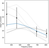 |
Fig. 9 Example spectral line energy distribution used for fitting the temperature toward the blue lobe of outflow A. The data (black circles with errorbars) are at CO transitions (3–2), (4–3), (6–5), and (7–6). The model fits (dotted and solid line) from RADEX also include CO (5–4). The dotted line represents the best fit (χ2 = 1 ± 0.05) SLEDs fromthe RADEX grid. The solid line represents the average value for these best fit models in (for this example) SLED. This fit gives Tkin = 66 K. |
4 Infall, accretion, and the evolutionary status of SDC335
4.1 Cloud infall and protostellar accretion rates
Outflow momentum flux (Eq. (5)) is a proxy for the protostellar mass accretion rate, Ṁacc, since the driving force of outflows is thought to result from the conservation of angular momentum within an accreting system (Konigl & Pudritz 2000; Pudritz et al. 2007; Tan et al. 2014). A theoretical relation between FCO and Ṁacc equates the two values scaled by a material entrainment efficiency, fent, and the protostellar mass ejection rateand wind speed, Ṁw, vw (Duarte-Cabral et al. 2013, see their Eq. (4)). Following this form of the FCO to Ṁacc relation and assuming the same material entrainment efficiency and wind properties as these authors have done (fent = 0.5, Ṁw ∕Ṁacc = 0.15 and vw = 40 km s−1), we derive the mass accretion rates given in Table 5.
For outflows A and B, the Ṁacc derived from our FCO values are in the range of 8.7–64.8 × 10⁻⁵ M⊙ yr−1, at a fixed temperature of T = 20 K, and 11.5–85.4 × 10⁻⁵ M⊙ yr−1, for our derived temperatures (T = 53 − 62 K). For outflow C, values are lower at Ṁacc is 0.2 × 10⁻⁵ M⊙ yr−1 for T = 20 K and 0.3 × 10⁻⁵ M⊙ yr−1 at the derived temperature of T = 55 K.
The values for outflows A and B are at the higher end of inferred accretion rates from low-mass protostars, Ṁacc ~ 10−5 M⊙ yr−1, (e.g. McKee & Tan 2003; Hosokawa & Omukai 2009; Hosokawa et al. 2010) and are more typical of those inferred for high-mass protostars, 10−4−10−3 M⊙ yr−1 (see e.g. Zhang et al. 2005; Fuller et al. 2005; Beuther et al. 2013; Duarte-Cabral et al. 2013; Rosen et al. 2016, 2019; Goddi et al. 2020), from both observational and theoretical works reported within the literature. The value for Ṁacc of outflow C is very low and likely a consequence of the limited velocity range over which we are able to measure this outflow’s properties. Indeed, as noted in Sect. 3.1, the driving sources for all three of the observed outflows are known to be high-mass protostars owing to their association with 6.7 GHz methanol masers, so the derived Ṁacc for outflow C can act as a lower limit.
We now consider the total derived mass accretion, Ṁtot. acc, within SDC335. This value is calculated as the sum of all the derived Ṁacc values presented in Table 5, giving a Ṁtot. acc of 1.4 (± 0.1) × 10−3 M⊙ yr−1. With this value, an interesting comparison can be made with the derived mass infall rate, Ṁinf, for the whole SDC335 cloud. Peretto et al. (2013) calculated a value of Ṁinf ≃ 2.5(±1.0) × 10−3 M⊙ yr−1. These two values are comparable within the quoted errors, which would imply a near 100% efficiency of infalling material on cloud scales (~ few pc) being funnelled onto the accretion disk scale (≪0.1pc) and driving the outflows. We note, however, that this does not imply a 100% accretion of the inflowing material into the protostar. Anear continuous flow of material from large (cloud/filament) to smaller (clump/core) scales would be significant as it suggests that each core is acting as a sink within the cloud drawing material from all scales and, as such, would have implications for high-mass star forming models. The protostellar accretion rate is a characteristic of the whole forming cluster under competitive accretion models (Bonnell et al. 2001, 2004, 2007) but under core accretion models (McKee & Tan 2002, 2003; Tan et al. 2014), this is set by the properties of bound cores. It would appear that this result favours the former set of models.
Another interesting implication of these inferred accretion rates is that the three known protostellar sources in SDC335 would appear to be drawing the majority of the material onto themselves, suggesting that there is a limited amount of material available to start forming any additional protostars within the system. In ALMA observationsof the IRDC G28.34 P1, Zhang et al. (2015) found a lack of low-mass protostars compared to the expected number from a typical IMF. These authors concluded, after discounting migration of low-mass stars into the centre of the cluster, that the most likely scenario for this under-abundance was because the low-mass stars are yet to form. If this is true then SDC335 may hold an explanation, in that early onset high-mass star formation dominates the inflowing material budget depriving lower mass proto or pre-stellar cores from gaining mass and starting formation.
As the inclination angles of the observed outflow are the dominant factor in the error budget of these calculations, an additional study of the protostars in SDC335 is required to better constrain the outflow properties. For example, testing for the presence of rotation axes, indicative of accretion disks, within the sources would help further this investigation.
4.2 Evolutionary status of SDC335
The works of Duarte-Cabral et al. (2013), Maud et al. (2015) and van Kempen et al. (2016), for instance, have shown there is a linear (in log-space) relation between the molecular outflow momentum flux (and therefore Ṁacc) and source luminosity in protostellar sources from low to high-masses. Recent numerical works by Rosen & Krumholz (2020) show this same trend.
Figure 10 plots the calculated outflow momentum flux as a function of source bolometric luminosity, Lbol, for the protostars in SDC335 and other sources, both low and high-mass, from the literature. The sources from the literature are low-mass Class 0 and I sources using values from Bontemps et al. (1996, and references therein) (both classes), observed and literature Class I sources from van der Marel et al. 2013, their Tables 4 and E.1, respectively. High-mass sources in the plot are Class 0 analogues from Duarte-Cabral et al. (2013) and high-mass protostellar sources from Maud et al. (2015).
The Lbol values for SDC335 are those derived in Paper I, and we divide the total luminosity of MM1 (1.82 × 10⁴ L⊙) between MM1a and MM1b in a 2.5:1 ratio (based on their respective optically thin radio emission flux ratios, see Paper I Table 5) yielding values of 1.3 × 10⁴ and 0.51 × 10⁴ L⊙ for MM1a and MM1b respectively. To compensate for this source of uncertainty each SDC335 point on Fig. 10 is presented with a ±50% error bar on the Lbol value. For outflows A and B the dominant source of error is the range of possible inclination angles, as such for these sources the errorbar represents the maximum and minimum values for FCO using the respective maximum and minimum possible inclination angles. For outflow C the FCO error includes the measured error on FCO, prior to inclination angle correction due to noise within the data, plus a ± 5 degree error on the inclination angle used (57.3° for the average angle for randomly orientated outflows).
We can see from Fig. 10 that all outflows in SDC335 fit the general trend of outflow momentum flux as a function of luminosity over the wide mass range represented. The plotted points are the sum of the red plus blue lobes for each source in SDC335, using the temperatures from our RADEX fitting and derived optical depth values in the calculation of the FCO values. The outflows A and B in SDC335 reside in the same parameter space as the high-mass protostars from Maud et al. (2015) with outflows A amongst the higher FCO range for its calculated Lbol. We note that the sources from Maud et al. (2015) are studied with a single dish instrument, thus lacking the resolution of our current work, leading to the question posed by those authors regarding whether or not their observed outflows are driven by a single or multiple objects. SDC335 outflow C has a significantly lower FCO value away from the proposed observed trend seen within the literature. This suggests either it has a less powerful, potentially more evolved outflow or this effect could simply be an artefact caused by the limited velocity range we are able to integrate over for this outflow coupled with a poorly defined inclination angle.
Assuming each of the identified outflows in SDC335 represents a single protostellar object, we can consider whether these sources represent an analogue of the protostellar source evolution classifications used at lower mass (Lada 1999). To this end, we generate best linear fit lines for the FCO as a function of Lbol for Class 0 and I sources using values from the literature plotted in Fig. 10. The best fit lines are plotted as the red dotted line for Class 0 and blue dashed-dot line for Class I, extended to higher luminosity values for comparison with SDC335 with associated 1-σ error margins from the fit plotted as shaded regions of matching colour.
The derived best fits are,
![\begin{equation*} \log_{10}(F_{\textrm{CO}}[{\textrm{Class}\ 0}])\,{=}\,{-}4.3({\pm}0.15) + 0.60({\pm}0.08)\log_{10}\left(\frac{{L}_{\textrm{bol}}}{{L}_{\odot}}\right) \end{equation*}](/articles/aa/full_html/2021/01/aa36043-19/aa36043-19-eq18.png) (6)
(6)
![\begin{equation*} \log_{10}(F_{\textrm{CO}}[{\textrm{Class}\ \textrm{I}}])\,{=}\,{-}5.3({\pm}0.12) + 0.63({\pm}0.16)\log_{10}\left(\frac{L_{\textrm{bol}}}{L_{\odot}}\right) \end{equation*}](/articles/aa/full_html/2021/01/aa36043-19/aa36043-19-eq19.png)
for Class 0 and I sources, respectively. We note that the best-fit line for Class 0 objects matches very closely to the results reported by Cabrit & Bertout (1992) for a sample of Class 0 sources (IRAS 16293, IRAS 3282, L1448, L1455M, RNO 43 and VLA1623) and a single high-mass object (G35.2 N).
The fitted lines show a decrease in outflow momentum flux between the Class 0 and I stages, as would be expected during the evolution of a protostellar source along the plotted evolutionary tracks (Duarte-Cabral et al. 2013) assuming a decreasing and intermittent accretion rate. From Fig. 10 we see that both MM1a and MM1b lie very close to the Class 0 best fit line and within the 1-σ error bound of that line of best fit (red shaded region). This suggests that these sources are very high-mass Class 0 analogue. We use the qualifier ‘very’ to indicate ’more extreme than’ based on a comparison to the position of the other high-mass Class 0 protostars in Fig. 10 from Duarte-Cabral et al. (2013) (empty star markers in the figure).
Supporting the ‘young, very high-mass’ status of the SDC335 sources MM1a and MM1b, we can see from the evolutionary tracks in Fig. 10 that these sources sit well above the 50 M⊙ track, but at an early stage before ~50% of the envelope mass has been accreted (denoted by the first arrow head). This is also corroborated by the short dynamical times of these outflows (few × 103 yr) in Table 4.
Paper I found, based on their current radio continuum properties, that the three high-mass protostellar objects in SDC335 are all currently displaying characteristics of zero age main sequence (ZAMS) stars of spectral type B1.5 (or B1.5-B1 for MM1a), which equates to stellar masses of ~ 9.0 M⊙ (Mottram et al. 2011). These relatively low ‘current’ stellar masses agree with the position of the observed outflow properties for A and B in terms of their position along the evolutionary tracks.
 |
Fig. 10 Outflow momentum flux, FCO, as a functionof powering source bolometric luminosity Lbol. Data for outflows A, B, and C in SDC335 are indicated by the filled squares and associated errorbars. The origin of the errorbars are discussed in the main text. The filled and empty hexagons are the Class 0 and Class I low-mass protostars from Bontemps et al. (1996). The diamonds are low-mass Class I sources from observation of Ophiuchus (van der Marel et al. 2013). Filled and empty triangles are literature values for Class 0 and I objects used by van der Marel et al. (2013, see their Table E.1). The stars denote the Duarte-Cabral et al. (2013) high-mass Class 0 analogues and the triangles are outflows from high-mass protostellar objects observed from the RMS survey (Maud et al. 2015). The green dashed tracks with arrow heads are the evolutionary tracks for decreasing or intermittentaccretion from Duarte-Cabral et al. (2013). The arrow heads represent the point at which a protostar of a given mass (given at the end of the arrow) has accreted 50 and 90% of their envelope mass. Red dotted line is the best fit to the plotted Class 0 sources extended to high luminosity with the red shaded region given the 1-σ error margin for this fit. The blue dashed-dot line and shaded region are the same but for the best fit to the plotted Class I sources. |
4.2.1 Low bolometric luminosities in the MM1 core
An open issue from previous work on SDC335, presented in Paper I, was the discrepancy between the observed bolometric luminosity Lbol, as derived from the millimetre core spectral energy distributions, and the luminosity of a ZAMS star of the spectral type necessary to produce the Lyman α photon flux inferred from the radio continuum, LZAMS. The value of Lbol was found to be approximately a factor 20 less than LZAMS.
To briefly review the Paper I finding (for more details, see their Sect. 4.1); the authors calculated a Lyman α photon flux based upon the HCH II continuum flux density for each of the three HCH II sources. From this, a ZAMS spectral type was associated with each core (B1.5 for MM2 and MM1b and B1 − B1.5 for MM1a) using values from Mottram et al. (2011) and Davies et al. (2011).
The ZAMS is reached when hydrogen burning has commenced, however, given the outflow indicators (masers, EGO etc.) present in SDC335, it was assumed in Paper I that each HCH II region represented a protostar which was still actively accreting. This assumption is borne out by the detection of the three outflows in the current work. An actively accreting protostar will have a total luminosity (assuming ZAMS properties), Ltot,ZAMS, which is the sum of its intrinsic luminosity, L*, and that from accretion, Lacc. Here Lacc is of the form  , and the value of M*, R* and L* were based on the ZAMS properties and Ṁ* (the mass accretion rate) was assumed to be equal to the global infall rate of SDC335 derived by Peretto et al. (2013) of 2.5 × 10⁻³ M⊙ yr−1.
From this calculation, the authors noted that the ZAMS L* and Lbol agree to within a factor of ~ 2 however this did not allow for ongoing accretion. Including Lacc gives Ltot,ZAMS a value that is a factor 20 higher than Lbol (see the values in Tables 2 and 6 of Paper I).
Paper I presented two scenarios which could account for the observed low bolometric luminosity from all three protostars in SDC335. In light of the data presented in this current work we can review these scenarios. The first scenario was that the assumed accretion rate 2.5 × 10⁻³ M⊙ yr−1 from Peretto et al. (2013) was too high and that the protostars were undergoing accretion at a lower rate (either overall or asa function of periodic accretion). In this current work, we derive a mass accretion rate onto each protostellar object from their outflow momentum flux (Col. 8 in Table 5) and find that indeed the values are lower than the Peretto et al. (2013) infall rate. This allows us to revise the values of Ltot,ZAMS from Table 6 of Paper I and address the second scenario discussed by those authors. In doing so, using both the minimum and maximum Ṁacc for each outflow from Table 5 to give a possible range of Ṁacc (and using the derived temperatures from Sect. 3.2.3), we provide revised values for Table 6 in Paper I in our current Table 6.
For MM2, the Ltot,ZAMS is now a factor ~2 lower than the Lbol which is consistent within the uncertainties on these values. A spectral type B1.5 ZAMS star has a mass of ~ 9 M⊙ (Mottram et al. 2011), which for MM2 would also agree with the accreting protostars position on the evolutionary tracks in Fig. 10 and its status as a potentially more evolved protostar than the cores in MM1.
In the case of the two ionising sources in MM1, the derived mass accretion rates cover a large range of values, 14.7 to 85.4 × 10⁻⁵ M⊙ yr−1 and 11.5 to 24.7 × 10⁻⁵ M⊙ yr−1 for MM1a and MM1b, respectively. With these values the bolometric luminosity for MM1a is consistent with Ltot,ZAMS at the lowest Ṁacc values but the discrepancy persists over the majority of the possible range (any value above 30.0 × 10⁻⁵ M⊙ yr−1 leads to a factor 2.5 discrepancy between the two luminosities). And for MM1b the discrepancy between Lbol and Ltot,ZAMS is at a factor of about three over the entire range – meaning that the observed Lbol < Ltot,ZAMS from Paper I also persists for this source.
The second scenario to account for the luminosity discrepancy discussed in Paper I is based upon the models of massive protostellar evolution at high accretion rates (~ 10−3 M⊙ yr−1) of Hosokawa & Omukai (2009) and Hosokawa et al. (2010). In this model massive protostars go through a phase of swelling to radii of ~ 100 R⊙ when their mass is between 6 and 10 M⊙, followed by a short contraction phase as their mass grows to between 10 and 30 M⊙. During the period of swollen radii the effective temperature of the protostar is lower than that of an equivalent mass ZAMS star, as such there are insufficient UV photons to generate a H II region. However, during the short contraction phase as the radius decreases the effective temperature increases and a H II region can form, whilst the radius remains somewhat swollen (~ 10 R⊙) giving a lower luminosity than a ZAMS star at the same mass. In Paper I, the authors suggest that each SDC335 protostar was in the contraction phase, accounting for both the observed H II regions and the low bolometric luminosities, though given the relatively brief duration of the contraction phase having multiple sources at this stage simultaneously would be unlikely.
The new derived mass accretion rates for MM1a and MM1b have values that are in the range of those considered by the Hosokawa & Omukai (2009) models (although for the swollen radii at accretion rates of ~ 10−4 M⊙ yr−1, the swelling is to ~ 40 R⊙ rather than 100 R⊙) and thus these sources are in either the swollen radii phase or the contraction phase – this would still seem a viable scenario that would lead to the lower observed luminosities. Given the relative lengths of each of these phases, it would be more likely that they are still in the swollen radii phase. If this is the case, the origin of the ionised emission in each core would then require an alternate explanation, which we address in Sect. 4.2.2.
Calculated luminosity values for the three protostellar cores in SDC335, assuming the ZAMS properties associated with each source in Paper I.
4.2.2 An alternate interpretation of the ionised radio continuum emission in SDC335
As discussed briefly in Paper I, the spectral indices for MM1b and MM2 fall within the range of values for both photo-ionised H II regions and collimated ionised jets (Reynolds 1986). Given the detection in this work of outflows from both these sources, it is important to review origin of radio continuum emission from the SDC335 protostars.
Radio continuum emission has been detected toward a number of low luminosity sources driving molecular outflows, for example in Anglada (1995). In this work, the author shows that the low luminosity for their sample of objects precludes the origin of the observed radio continuum emission coming from photoionisation by Lyman alpha photons. Using the models of shock ionised gas from Curiel et al. (1987, 1989), the author then shows that for their sample, shock ionisation is capable of creating the observed radio continuum based on the outflow momentum flux of their targets.
Based upon the best-fit model and data in Anglada (1995, their Eq. (1) and Fig. 5) we find that using their 8, 23, and 25 GHz flux densities Paper I, MM1a and MM1b are shown to reside between the line of minimum requirement (dashed line in Anglada 1995 Fig. 5) and the line of best fit (solid line in Anglada 1995 Fig. 5) for shock ionisation as the mechanism for the observed radio continuum emission in their sample. This suggests that for these sources this may indeed be the origin of the detected radio emission. However, MM2 is a factor of between ~ 17 and 37 below the lower bound of the emission expected from shocks (Anglada 1995). This may be an evolutionary factor or one arising from the orientation of the MM2 outflow to the line of sight, which limits the range of velocities we are able to integrate over leadingto an underestimate of the outflow momentum flux value for this source (Sect. 4.1).
The direct implication of interpreting the origin of the ionised matter as from outflow shocks as opposed to photoionisation is the evolutionary status of the protostellar sources themselves. If the emission is not due to photoionisation, this suggests that the protostars are at an earlier pre-ionising stage in their evolution.
It is important to state that although this alternate interpretation may account for the presence of ionised hydrogen and indicate a resolution of the discrepancies between observed bolometric luminosity and a corresponding ZAMS luminosity, the protostars within SDC335 remain high-mass protostellar sources, which will go on to form stars of mass > 8M⊙. We base this on both their observed luminosities (of the order 104 L⊙ Paper I) and the co-location of each of the radio emission peaks with 6.7 GHz methanol maser emission. Higher spatial resolution (≤ 2.0 ′′) observationsof SDC335 at radio frequencies would be required to fully assess this interpretation. The impact on the current work – should theradio free-free emission prove to be outflow shocks – is limited to the discussion in Sect. 4.2.1. All other results would remain unchanged.
5 Interaction between outflows and filaments
Previous studies of the motion of material at large scales in SDC335 have found that the cloud is both globally collapsing toward its centre and that material is being transported inward to this region along the filamentary arms of the cloud (Peretto et al. 2013). In our current work, however, we report the detection of material outflowing from the protostellar cores at the cloud centre. In this section, we look at the evidence of the interaction of the filamentary infalling and outflowing material. Finding regions of interaction within SDC335 would make the IRDC a valuable source for studying the potential disruptive effects on material transport from feedback of young massive stars have. In the following, we highlight the observed features within SDC335 that mark potential filament-outflow interactions. As part of this discussion, we identify each outflow lobe by the letter corresponding to the outflow and a sub-script colour to indicate the particular red or blue lobe.
5.1 ClassI methanol masers
Collisionallyexcited Class I methanol masers are commonly associated with molecular outflows in regions of massive star formation (e.g. Kurtz et al. 2004; Cyganowski et al. 2009). SDC335 was known to harbour four Class I maser sources (Paper I, and references therein), all of which are clearly spatially offset from the compact H II regions in the MM1 and MM2 cores. With our new, more sensitive data, an additional four individual maser sources were detected. The spectrum of each maser is presented in Fig. 11. Figure 12 presents the maser locations within SDC335, with the masers colour-coded by velocity.
All the maser spots peak at velocities within ~ 6.0 km s−1 of the systemic velocity of the SDC335 mm-cores. The position and peak emission properties of each spot are given in Table 7. The masers are numbered from south to north. Whilst we do not focus on the properties of each maser spot individually within this work, we include in the following discussion the maser spots that provide useful indications as shock tracing when interpreted as potentially part of the outflow-filament interactions within SDC335.
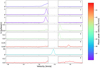 |
Fig. 11 Spectra taken at the peak position of the eight Class I methanol masers observed toward SDC335. Each panel gives the spectra of an individual maser spot (numbered in the upper right of the panel). Each spectra is colour coded by its peak velocity following the colour bar (right). The y-axis for each spectrum differs and is scaled to between −0.1 × and 1.1 × the peak flux density of the individual maser as listed in Table 7. The velocity range − 47.0 to − 43.8 km s−1 is blanked outin panels 1–6 and 8 as between these velocities the spectra of these masers are dominated by imaging artefacts caused by the strong emission from maser 7. This is to avoid confusion between true maser emission and imaging artefacts. |
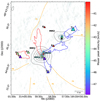 |
Fig. 12 SDC335 region showing the position of the Class I methanol masers. Orange dashed lines as per Fig. 1. Filled triangles, the Class I methanol masers detected in the ATCA data, colour-coded by velocity matching that in Fig. 11, the size of the triangle is proportional to the flux density of the maser source. Cyan ‘ × ’ denote the location of Class II methanol masers at 6.7 GHz and yellow ‘+’ denote the H2O masers at 22 GHz. Grey contours show the ALMA 3 mm continuum emission and the greyscale images shows the ATCA 8 GHz continuum emission. The red and blue contours show ~ 9% of the peak integrated intensity of each of outflow, using the velocity ranges from Table 2 as a guide when comparing the maser positions. |
5.2 Interaction regions
5.2.1 ABlue and the F3 and F4 filaments
The ABlue outflow is well collimated near the driving source (MM1a) when observed at high resolution (ALMA CO and 13CO), as seen in the narrow structure of the contour plots in Fig. 2Azoom and the CO velocity channel maps shown in Fig. 13. The shock-tracing SiO emission detected in this outflow lobe is however predominately at the end (furthest from the driving source) of this lobe Fig. 2B.
This region of SiO emission and the observed lobe end in the CO and 13CO ALMA observation coincide spatially and kinematically with the ends of the F3 and F4 filaments of the IRDC (marked as the orange dash line in Figs. 1 and 2, cf. Peretto et al. 2013). The F3 and F4 filaments are carrying material into the SDC335 central region at velocities of ~ − 45.8 and − 46.5 km s−1 respectively (see Peretto et al. 2013, their Figs. 4c and 5). Given the Vlsr of the MM1a core, these infalling velocities are moving in the opposite direction to the outflowing material (VAblue ~ −50.5 to −82.4 km s−1, see Figs. 13 and 2). Supporting this interpretation is the position and velocity range covered by the Class-I CH3OH maser source 1 (see Table 7). We show the presence of the maser spot at a given velocity in Fig. 13 as a solid purple circle.
Given the collisionally excited pumping mechanism responsible for Class-I masers and the hypothesis that such collisional excitement occurs at the interfaces of outflows and the surrounding molecular gas as seen in, for example, Plambeck & Menten (1990); Kurtz et al. (2004); Voronkov et al. (2010), the alignment of the maser activities both spatially and kinematically with the outflow lobe end suggest that we are indeed seeing the point of interaction between the ABlue outflow andthe infalling material from the F3 and F4 filaments. The large velocity range the CH3OH emission covers requires a strong shock front to pump such maser emission.
5.2.2 C and the F2 filament
The one detected lobe of outflow C (Cblue) exhibits both the brightest Class I methanol maser (maser 7, Table 7) and the brightest SiO emission detected in the region (see Fig. 6). At a peak flux density of 48.78 Jy, maser 7 is over 40 times the intensity of any of the other detected maser sources (see e.g. Fig. 11). Given that both SiO emission and Class I CH3OH maser are shock tracing species we note that the end (away from the driving source MM2) of this outflow lobe (Fig. 2) appears close to the fiducial end of the F2 filament (orange dashed line, cf. Peretto et al. 2013). This suggests that we are observing a shocked region caused by the meeting of the outflow and the inflowing matter from the F2 filament. The velocities of Cblue and the infall along F2 are in opposite directions, with the F2 filament VF2 = ~−46.0 km s−1 (see Peretto et al. 2013,their Figs. 4c and 5), so redder than the Vlsr of MM2 and  = −59.1 to –43.6 km s−1, thereby extending both red and blue-ward of this Vlsr. Although the maser position and the end of the orange dashed line representing F2 in Figs. 2A–C do not match exactly, we emphasise that the dashed line is a fiducial marker and the true morphology and kinematics at the end of the inflow are not known at spatial resolutions better than ~ 5′′ (Peretto et al. 2013). Further higher resolution observations of the region would be required to confirm this as a true shock-interaction region.
Characteristics of observed Class I CH3OH masers.
5.2.3 Curvature of Ared and the F1 filament
The Ared lobe is observed in our CO (ALMA), SiO, and HNC data to exhibit curvature at its northernmost end. Inspecting the position of the nearby filamentary arm, F1, in Fig. 2 it appears that the curvature coincides with where Ared would meet the infalling material from the filament. Emission from the Ared here is at velocities of ~−30 to −20 km s−1 (CO, SiO) whereas the inflowing material of the F1 filament is at ~ − 47.25 km s−1 (see Peretto et al. 2013, their Figs. 4c and 5). The start of curvature of the F1 filament also coincides with a clump of SiO emission and CO (beyond the velocity range used to generate the contours in Fig. 2A) offset from the outflow (see Fig. 2B) at velocities − 36.9 to − 41.2km s−1. This is spatially and kinematically coincident with maser 8 (see Table 7), suggesting an interaction point between the inflow and outflow is likely associated with a shock front leading to the SiO. Maser 8 peaks at −40 km s−1 with a velocity range ± ~ 3.0 km s−1 as such covers velocities which are between those measured for the inflowing and outflowing material. Figure 14 gives the spectra of CO and SiO at the position of maser 8.
5.2.4 Bred shocked emission
The Bred lobe is observed in SiO, HNC and CO (both APEX and ALMA). The leading edge of this outflowis coincident with the positions of masers 3 and 4 and peak SiO emission (see Figs. 2-A and B) of the outflow, indicating a region of shocked gas. We note that this lobe does not directly appear to be interacting with a filamentary inflow, but from Fig. 1 the outflow appears toward the edge of the 8 μm dark region of the cloud suggesting some interaction at the cloud boundary. In Figs. 15 and 16 we give the spectra of CO (ALMA), HNC and SiO at the position of masers 3 and 4.
5.3 A and B outflows misalignment, a potential scenario
As evident in Fig. 2 and noted in Sect. 3.1.3, outflows A and B have outflow axes that are approximately perpendicular to one another. Naively, one would assume that the angular momentum axes for a pair of protostars of similar mass separated by a relatively small distance (~ 9000 AU) would be aligned. This appears not to be the case for SDC335.
Within the literature, there are other examples showing similar misalignments. For example, protostars A and B within IRAS16293 (separated by 600 AU) were found to have rotation axes misaligned (Pineda et al. 2012, and references therein) with A observed edge on and B either having little to no observable rotation or a rotation axis in the plane of the sky. This gives A and B effectively a ~ 90° offset in their angular momentum axes. Similarly, there are several systems found in Perseus (with pairs separated by 1000 to 10 000 AU) which show outflow axes that are misaligned between low mass protostars with the distribution of axes appearing to prefer random or anti-aligned orientations (Lee et al. 2016).
We consider a possible cause for this misalignment in SDC335. This scenario posits that the outflow progenitors MM1a and MM1b, after fragmenting from the MM1 mm-core, have grown in mass by accreting matter from different material flows arriving at each core from different directions, thus changing their respective angular momentum vectors as the system evolves. The high, non-uniform accretion rates inherent to massive star formation (Ṁacc ~ 10−3 M⊙ yr−1) will push the star around and cause the angular momentum vector to precess. Such behaviour has been seen in three-dimensional (3D) radiation-magnetohydrodynamic (RHD) simulations of the collapse of a turbulent massive pre-stellar core into a massive star (Rosen et al. 2016; Rosen & Krumholz 2020). The movement of the star and its angular momentum vector will cause the outflows to be launched over a larger area as the star grows in mass. This effect will broaden the entrained outflows since the protostellaroutflows are likely launched along the star’s or surrounding accretion disk’s angular momentum vector (e.g. Shu et al. 2000; Pudritz et al. 2007).
Figure 17 (adapted from Rosen & Krumholz 2020) shows two snapshots from a 3D RHD simulation that models the collapse of a turbulent massive (150 M⊙) pre-stellar core into a massive stellar system and includes radiative feedback and collimated outflows that are launched along the stars’ angular momentum vectors (see subgrid model description by Cunningham et al. 2011). These snapshots show the column density of the molecular material that is entrained by the protostellar outflows from the stars that have formed. To obtain the distribution of entrained material, we compute the mass-weighted integrated gas density only along cells that have ρOF∕ρ ≥ 0.1, where ρOF is the outflow gas density injected by stars, and ρ is the total gas density.
In the first snapshot, where the time elapsed is 0.4 tff where tff = 42.7 kyr is the core’s free-fall timescale, the star has a mass of 9.12 M⊙ and what looks like multiple molecular outflows. However, this outflow morphology is due to the non-uniform accretion flow that knocks the star around, causing the star to move away from its birth site and precess; thereby causing the outflow launching direction to change with time. At later times, t = 0.6tff, when multiple low-mass protostars have formed and are clustered near the massive protostar (pink filled-in circles), the smaller and weaker multiple outflows from the low mass protostars overlap. The resulting overlapping entrained outflows from these clustered low-mass companions to the right of the primary star are inclined by ~ 45° to the entrained outflow from the primary star, as indicated by the arrow in Fig. 17. We note that this significant offset between outflow axes and separation between the massive and low-mass stars is similar to what is seen in SDC335. The fact this is occurring within less than one cloud free-fall time for the simulated cloud lends further credence to SDC335 being at an early period of star formation. (For SDC335 tff ~ 3.5 × 10⁵ yr.)
Measuring the level of turbulence of material within the central region of SDC335 and the accretion flows onto individual cores would require higher resolution observations of the dense gas (combined with single-dish data to avoid ‘missing spacing’ problems), which are not currently available.
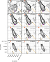 |
Fig. 13 Channel map of the CO emission from the ABlue outflow. The velocity of each image is listed in the upper right corner. The position of MM1a isindicated by the red star. The purple filled circle gives the position of the Class I CH3 OH maser source 1 (see Table 7), only at velocities where the maser is present. The orange dashed lines show the fiducial directions of the F3 and F4 filaments as per Fig. 1. Contours are plotted at the 5,10, 20, 40, 50, 60, 70 and 80 σ level of the ALMA CO image (where σ = 22.0 mJy bm−1). |
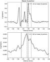 |
Fig. 14 CO and SiO spectra measured at the position of the maser 8 peak emission see Table 7. The vertical dashed line gives the Vlsr of the targetand the vertical dotted lines mark the range in velocity of the clump of emission seen toward the curvature of the Ared outflow lobediscussed in Sect. 5.2.3. The vertical dash-dot line gives the velocity of peak emission from maser 8. |
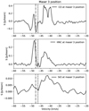 |
Fig. 15 CO (ALMA), HNC and SiO spectra measured at the position of the maser 3 peak emission see Table 7. The vertical dash-dot line gives the velocity of peak emission from maser 3 and the vertical dashed line the Vlsr of the outflow driving source, MM1b. |
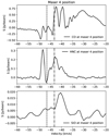 |
Fig. 16 CO and SiO spectra measured at the position of the maser 4 peak emission see Table 7. The vertical dash-dot line gives the velocity of peak emission from maser 4 and the vertical dashed line the Vlsr of the outflow driving source, MM1b. |
6 Discussion and conclusions
Using new ATCA SiO and CH3OH observations coupled with archival CO, 13CO, and HNC data from ALMA and four transitions of CO from the APEX telescope, we identify and analyse three molecular outflows within the young high-mass star forming infrared dark cloud SDC335. These data have yielded the following outcomes:
-
The three outflows, A, B, and C, are identified, each associated with one of the three known HCH II regions in SDC335 (Paper I) (MM1a, MM1b, and MM2, respectively). The red-blue outflow lobes from A extend in the north-south direction, B extends east-west and C, of which only the blue lobe is detected, extends to the north-west. They have a full width velocity ranges of up to 10 km s−1 and temperatures of ~60 K. The two most massive sources in the cloud, MM1a and MM1b, are separated by ~9000 AU but have driving outflows of projected outflow axes that are approximately perpendicular to one another. The blue lobe of outflow A displays a structure and velocity that is characteristic of a jet.
-
The analysis of the measured outflow momentum flux, FCO, as a function of source bolometric luminosity, Lbol, and in comparison to theoretical evolutionary tracks (Duarte-Cabral et al. 2013) confirms that the progenitor protostars are massive young stellar objects with two sources residing above the tracks for 50 M⊙ stars. Using samples of FCO and Lbol measurements from the literature for low to intermediate mass stars at evolutionary classes 0 and I, we derived best-fit FCO-Lbol relations for these two classes. Extrapolating these relations upward in Lbol, we find the outflow momentum flux properties of the SDC335 outflows A and B agree best, with their progenitors being high-mass Class 0 analogues and indicating that SDC335 is at a very early stage of the star-formation process.
-
Inferring the mass accretion rates from the source outflow properties, we find that the total mass accretion is 1.4(±0.1) × 10−3 M⊙ yr−1 on the protostellar scale. This value is consistent with the calculated mass infall rate on cloud and filamentary scales 2.5(±1.0) × 10−3 M⊙ yr−1 found by Peretto et al. (2013). This result suggests that at this early stage of evolution nearly all the material accreted onto the clump is funnelled through the cores onto these three massive young sources, limiting the scope for the formation of additional, low mass sources in the region. If significant numbers of lower mass stars are to form in SDC335, these would then have to form at a later stage in the evolution of the region.
-
These new data combined with existing knowledge of the bulk inflow and global and filamentary collapse properties of the SDC335 cloud provide compelling evidence of the interaction between the molecular outflows and the material infalling along the filamentary arms. Given the very young (Class 0 analogue) status of the protostars driving the outflows, this makes SDC335 a valuable test bed for study of the disruptive feedback effects of massive protostars on their natal clouds.
The observed properties described in this work make the infrared dark cloud SDC335 a key target for the more detailed study of how massive protostars form and effect their natal environments through accretion and protostellar outflows. Such features warrant further study at high spectral and spatial resolutions and sensitivities.
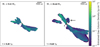 |
Fig. 17 Projection plots generated from simulations of high-mass star forming regions, (adapted from Rosen & Krumholz 2020). These plots show only the material contained in the systems outflows in the condition |

Acknowledgements
The Australia Telescope Compact Array is part of the Australia Telescope which is funded by the Commonwealth of Australia for operation as a National Facility managed by CSIRO. The authors would like to thank all ATNF staff past and present who helped during the ATCA observation used in this paper, particularly those who provided A.A. with curry. The authors would also like to thank the anonymous referee for their input into the paper after initial submission which has helped to improve the work. This paper makes use of the following ALMA data: ADS/JAO.ALMA#2011.0.00474.S and #2012.0.00781.S. ALMA is a partnership of ESO (representing its member states), NSF (USA) and NINS (Japan), together with NRC (Canada) and NSC and ASIAA (Taiwan), in cooperation with the Republic of Chile. The Joint ALMA Observatory is operated by ESO, AUI/NRAO and NAOJ. This publication is based on data acquired with the Atacama Pathfinder EXperiment (APEX). APEX is a collaboration between the Max-Planck-Institut fuer Radioastronomie, the European Southern Observatory, and the Onsala Space Observatory. A.A. is funded by the STFC at the UK ARC Node. G.A.F acknowledges financial support from the State Agency for Research of the Spanish MCIU through the AYA2017-84390-C2-1-R grant (co-funded by FEDER) and through the “Center of Excellence Severo Ochoa” award for the Instituto de Astrofísica de Andalucia (SEV-2017-0709). N.P. wishes to acknowledge support under STFC consolidated grants ST/N000706/1 and ST/S00033X/1. A.D.C acknowledges the support from the UK STFC consolidated grant ST/N000706/1. A.L.R acknowledges support from NASA through Einstein Postdoctoral Fellowship grant number PF7- 180166 awarded by the Chandra X-ray Center, which is operated by the SmithsonianAstrophysical Observatory for NASA under contract NAS8-03060. This research made use of APLpy, an open-source plotting package for Python hosted at http://aplpy.github.com. This research made use of Astropy (http://www.astropy.org), a community-developed core Python package for Astronomy (Astropy Collaboration 2013, 2018).
Appendix A Spectra of the outflow driving sources
To compliment the outflow spectra in Figs. 3–6, we present in Figs. A.1 and A.2 spectra over the same velocity range at the peak position of the three HCH II regions in SDC335. These are the likely driving sources of the outflows, as described in the main text.
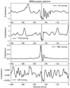 |
Fig. A.1 Spectra at the position of peak emission at 23 GHz (Avison et al. 2015) from the MM1a HCH II region at the same CO, 13CO, HNC, and SiO frequency tunings, as shown in Figs. 3–6. The vertical dashed line gives the Vlsr of the HCH II. |
Appendix B Inclination angle considerations based on observed length-to-width ratio
Here, we address the arguments used to limit the range of possible inclination angles derived from the Cabrit & Bertout (1986) models by introducing a general outflow model beyond the simple bicone.
Following Fig. B.1, we define the length, L, of an outflow as from the driving source to the end of the outflows influence on the surrounding medium in the direction of the outflowing material. Complementary to this, the outflow width, W, is the maximum extent of the outflows influence orthogonal to the outflow direction. The angle between the axis of symmetry of the outflow (along L) and the widest point, called the opening angle, we denote here as θ. The distance along L to the point of maximumwidth we name x. The length of x depends on the morphology of the outflow. In the case of the Cabrit & Bertout (1986) bicone model L = x. The true length-to-width, LWR, of the outflow is then defined as  .
.
Also presented in Fig. B.1 are the observed properties of the outflow. The observed length LO of the outflow at an inclination angle, i, with respect to the observer is the sum of the contribution of the outflow wall or edge, EO, and emission from the outflow cavity/dome end, CO. So, LO = EO + CO.
In turn EO comprises the sum of the outflow wall from it origin to length x,  and from the wall from x to the end of the outflow at L,
  . These two contributions have the forms:
 (B.1)
(B.1)
 (B.2)
(B.2)
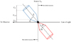 |
Fig. B.1 Schematic of the parameters for a generalised, non-bicone, outflow model used to limit the possible inclination angles for outflows A and B. |
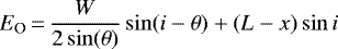
and the contribution of the cavity along the line of sight is given by,
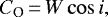 (B.4)
(B.4)
such that in its full form the observed length is given by
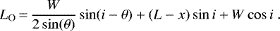 (B.5)
(B.5)
We note that inclination projection effects on W are minimal, for example, given a source at distance of 3 kpc the observed width only differs from the true W due to its inclination at the 0.02% level for L = 0.5pc (larger than any measured or corrected length in our observed outflows) when inclined along the line of sight. Indeed, an outflow of L = 30 pc inclined along the line of sight will only have a project effect difference on W at the 1% level. As such, we neglect this consideration. This gives the observed length-to-width as LWR . There is a final observable counterpart to the true physical value which is the observed length from the driving source to the widest point, xO which is given by xsini.
B.1 Bicone case, L = x
In the case that the outflow has a biconical morphology, as is the case assumed to derive our initial inclination angle ranges, then L = x and the second term in Eq. (B.5) becomes zero. This leads the observed length-to-width to become:
 (B.6)
(B.6)
from which using the measured LWRO and θ it is possible to constrain the value of inclination angle, i. For outflow A with a θ = 11° and LWRO = 3.5, Eq. (B.6) asymptotes at 79° with a LWRO = 2.6. Similarly for outflow B with a θ = 14° and LWRO = 3.0 asymptotes at 76° with a LWRO = 2.1. In both cases, these asymptotes are clearly at 90° – θ. Based on this, it becomes clear that whilst the biconical morphology does not apply particularly well to outflows A and B, the observed length-to-width ratios are providing evidence that (in the absence of external influence on the morphology) these outflows tend toward higher inclination angles.
B.2 General case, L ≠ x
For the general case, where L≠x, the inspection of the inclination angle now depends on an additional piece of information, the observed distance from the outflow origin to the point that the outflow is widest, xO. With this the observed LWRO becomes,
 (B.7)
(B.7)
Given our observed LO, W, θ and xO, we can solve numerically the range of i and x values that will return a LWR matching our observed values. We do this for a model outflow of L = 1 with x and W as fractions of this. For this work, we consider values of i and x which return both an xO and LWRO within ±10% of our observed values.
Under these conditions we find that we can limit the range of i values to between 53 and 76° for outflow A and 59 and 89° for outflow B. The latter values can again be limited at the higher end by kinematics, as above 79° we would observe both red- and blue-shifted emission at either side of the driving source for outflow B, giving us a final limit for B of between 59 and 79°. These are significantly smaller ranges than using the Cabrit & Bertout (1986) models and again tend to higher inclination angles.
B.3 Implications of using the bicone model
In Sect. 3.2.2, the morphology described in Appendix B.2 is used in place of the typical biconical outflow morphology to narrow the ranges of potential inclination angles for outflows A and B observed in SDC335. Table 3 provides the factors required to correct the observed values for the effects of inclination. These correction factors are given for both the angle ranges generated using our preferred morphology and the bicone case.
Owing to the difference in angles covered the correction factors differ between the two morphologies by factors of 0.65 and 2.15 for outflow A and 0.6 and 2.65 for outflow B, respectively. One item that is of significance with regard to the findings of this paper is the correction factor applied to the momentum flux, F. Using the bicone morphology, the momentum flux values are 2.15 × and 2.65 × smaller for outflows A and B, respectively. Following this reduction through our analysis yields the following changes:
– The FCO values for MM1a and MM1b become 1161.8 × 10−5 and 341.3 × 10⁻⁵ M⊙ km s−1 yr−1, respectively (for the sum of the red and blue lobes), leading to each source being lower on the y-axis of Fig. 10. MM1a remains consistent with the Class 0 line of best fit whereas MM1b moves to the upper end of the 1 − σ error margin for the Class I line of best fit, suggesting it is potentially more evolved than MM1a though remains consistent with the Class 0 line within errors. Both sources remain consistent with the 50 M⊙ evolutionary track plotted in Fig. 10.
– The Ṁacc derived from our FCO values are now in the range 6.8–39.6 × 10⁻⁵ M⊙ yr−1, at T = 20 K, τ = 3.5, and 4.3–9.3 × 10⁻⁵ M⊙ yr−1, for T = 53−62 K with τ = 8.2 for outflows A and B. From these, the total derived mass accretion, Ṁtot. acc, within SDC335 (as defined in Sect. 4.1) becomes 6.04(±0.04) × 10−4 M⊙ yr−1. This means the comparison to the total infall rate is somewhat weaker, at 24% of the Peretto et al. (2013) values, rather than 55% and comparable within the errors.
– The change in Ṁacc leads to a lessening of the discrepancy discussed in Sect. 4.2.1 between the bolometric luminosity, Lbol, and Ltot,ZAMS. For MM1b with Ltot,ZAMS, becomes a factor 1.5–2.4 times lower than Lbol, meaning these values are consistent (as is the case with source MM2). For MM1a range of Ṁacc values, an allowance remains for a discrepancy of greater than 2.5 × between the two luminosities at the higher end (> 30 × 10−5 M⊙ yr−1) of the derived range.
References
- Anglada, G. 1995, Rev. Mex. Astron. Astrofis. Conf. Ser., 1, 67 [Google Scholar]
- Arcé, H., Shepherd, D., Gueth, F., et al. 2006, Protostars and Planets V, eds. K. K. Bo Reipurth, & D. Jewitt (Tucson, AZ: University of Arizona Press) [Google Scholar]
- Astropy Collaboration (Robitaille, T. P., et al.) 2013, A&A, 558, A33 [NASA ADS] [CrossRef] [EDP Sciences] [Google Scholar]
- Astropy Collaboration (Price-Whelan, A. M., et al.) 2018, AJ, 156, 123 [Google Scholar]
- Avison, A., Peretto, N., Fuller, G. A., et al. 2015, A&A, 577, A30 [NASA ADS] [CrossRef] [EDP Sciences] [Google Scholar]
- Beuther, H., Schilke, P., Gueth, F., et al. 2002, A&A, 387, 931 [NASA ADS] [CrossRef] [EDP Sciences] [Google Scholar]
- Beuther, H., Linz, H., & Henning, T. 2013, A&A, 558, A81 [NASA ADS] [CrossRef] [EDP Sciences] [Google Scholar]
- Bonnell, I. A., Bate, M. R., Clarke, C. J., & Pringle, J. E. 2001, MNRAS, 323, 785 [NASA ADS] [CrossRef] [Google Scholar]
- Bonnell, I. A., Vine, S. G., & Bate, M. R. 2004, MNRAS, 349, 735 [NASA ADS] [CrossRef] [Google Scholar]
- Bonnell, I. A., Larson, R. B., & Zinnecker, H. 2007, Protostars and Planets V (Tucson, AZ: University of Arizona Press), 149 [Google Scholar]
- Bontemps, S., Andre, P., Terebey, S., & Cabrit, S. 1996, A&A, 311, 858 [NASA ADS] [Google Scholar]
- Braun, R., & Walterbos, R. A. M. 1985, A&A, 143, 307 [NASA ADS] [Google Scholar]
- Cabrit, S., & Bertout, C. 1986, ApJ, 307, 313 [NASA ADS] [CrossRef] [Google Scholar]
- Cabrit, S., & Bertout, C. 1992, A&A, 261, 274 [Google Scholar]
- Caswell, J. L., Fuller, G. A., Green, J. A., et al. 2011, MNRAS, 417, 1964 [NASA ADS] [CrossRef] [Google Scholar]
- Cunningham, A. J., Klein, R. I., Krumholz, M. R., & McKee, C. F. 2011, ApJ, 740, 107 [NASA ADS] [CrossRef] [Google Scholar]
- Cunningham, N., Lumsden, S. L., Cyganowski, C. J., Maud, L. T., & Purcell, C. 2016, MNRAS, 458, 1742 [NASA ADS] [CrossRef] [Google Scholar]
- Curiel, S., Canto, J., & Rodriguez, L. F. 1987, Rev. Mex. Astron. Astrofis., 14, 595 [Google Scholar]
- Curiel, S., Rodríguez, L. F., Cantó, J., et al. 1989, Astrophys. Lett. Commun., 27, 299 [Google Scholar]
- Cyganowski, C. J., Whitney, B. A., Holden, E., et al. 2008, AJ, 136, 2391 [NASA ADS] [CrossRef] [Google Scholar]
- Cyganowski, C. J., Brogan, C. L., Hunter, T. R., & Churchwell, E. 2009, ApJ, 702, 1615 [NASA ADS] [CrossRef] [Google Scholar]
- Cyganowski, C. J., Brogan, C. L., Hunter, T. R., Churchwell, E., & Zhang, Q. 2011, ApJ, 729, 124 [NASA ADS] [CrossRef] [Google Scholar]
- Cyganowski, C. J., Brogan, C. L., Hunter, T. R., et al. 2017, MNRAS, 468, 3694 [NASA ADS] [CrossRef] [Google Scholar]
- Davies, B., Hoare, M. G., Lumsden, S. L., et al. 2011, MNRAS, 416, 972 [NASA ADS] [CrossRef] [Google Scholar]
- Drabek-Maunder, E., Hatchell, J., Buckle, J. V., Di Francesco, J., & Richer, J. 2016, MNRAS, 457, L84 [NASA ADS] [CrossRef] [Google Scholar]
- Duarte-Cabral, A., Chrysostomou, A., Peretto, N., et al. 2012, A&A, 543, A140 [NASA ADS] [CrossRef] [EDP Sciences] [Google Scholar]
- Duarte-Cabral, A., Bontemps, S., Motte, F., et al. 2013, A&A, 558, A125 [NASA ADS] [CrossRef] [EDP Sciences] [Google Scholar]
- Duarte-Cabral, A., Bontemps, S., Motte, F., et al. 2014, A&A, 570, A1 [NASA ADS] [CrossRef] [EDP Sciences] [Google Scholar]
- Frank, A., Ray, T. P., Cabrit, S., et al. 2014, Protostars and Planets VI (Tucson, AZ: University of Arizona Press), 451 [Google Scholar]
- Fuller, G. A., Williams, S. J., & Sridharan, T. K. 2005, A&A, 442, 949 [NASA ADS] [CrossRef] [EDP Sciences] [Google Scholar]
- Garay, G., Brooks, K. J., Mardones, D., Norris, R. P., & Burton, M. G. 2002, ApJ, 579, 678 [NASA ADS] [CrossRef] [MathSciNet] [Google Scholar]
- Goddi, C., Ginsburg, A., Maud, L., Zhang, Q., & Zapata, L. 2020, ApJ, 905, 25 [CrossRef] [Google Scholar]
- Green, J. A., & McClure-Griffiths, N. M. 2011, MNRAS, 417, 2500 [NASA ADS] [CrossRef] [Google Scholar]
- Gueth, F., & Guilloteau, S. 1999, A&A, 343, 571 [NASA ADS] [Google Scholar]
- Güsten, R., Nyman, L. Å., Schilke, P., et al. 2006, A&A, 454, L13 [NASA ADS] [CrossRef] [EDP Sciences] [Google Scholar]
- Güsten, R., Baryshev, A., Bell, A., et al. 2008, Proc. SPIE, 7020, 702010 [CrossRef] [Google Scholar]
- Hosokawa, T., & Omukai, K. 2009, ApJ, 691, 823 [NASA ADS] [CrossRef] [Google Scholar]
- Hosokawa, T., Yorke, H. W., & Omukai, K. 2010, ApJ, 721, 478 [NASA ADS] [CrossRef] [Google Scholar]
- Kasemann, C., Güsten, R., Heyminck, S., et al. 2006, Proc. SPIE, 6275, 62750N [CrossRef] [Google Scholar]
- Klaassen, P. D., Galván-Madrid, R., Peters, T., Longmore, S. N., & Maercker, M. 2013, A&A, 556, A107 [NASA ADS] [CrossRef] [EDP Sciences] [Google Scholar]
- Klein, T., Ciechanowicz, M., Leinz, C., et al. 2014, IEEE Trans. Terahertz Sci. Technol., 4, 588 [NASA ADS] [CrossRef] [Google Scholar]
- Konigl, A., & Pudritz, R. E. 2000, Protostars and Planets IV, eds. V. Mannings, A. P. Boss, & S. S. Russell (Tucson, AZ: University of Arizona Press), 759 [Google Scholar]
- Kroupa, P. 2002, Science, 295, 82 [NASA ADS] [CrossRef] [PubMed] [Google Scholar]
- Krumholz, M. R., Bate, M. R., Arce, H. G., et al. 2014, Protostars and Planets VI, eds. H. Beuther, R. S. Klessen, C. P. Dullemond, & T. Henning (Tucson, AZ: University of Arizona Press), 243 [Google Scholar]
- Kurtz, S., Hofner, P., & Álvarez, C. V. 2004, ApJS, 155, 149 [NASA ADS] [CrossRef] [Google Scholar]
- Lada, C. J. 1999, The Origin of Stars and Planetary Systems, eds. C. Lada, & N. Kylafis (Berlin: Springer), 143 [CrossRef] [Google Scholar]
- Lee, K. I., Dunham, M. M., Myers, P. C., et al. 2016, ApJ, 820, L2 [NASA ADS] [CrossRef] [Google Scholar]
- Liu, J., Qiu, K., Wyrowski, F., et al. 2018, ApJ, 860, 106 [CrossRef] [Google Scholar]
- Maud, L. T., Moore, T. J. T., Lumsden, S. L., et al. 2015, MNRAS, 453, 645 [NASA ADS] [CrossRef] [Google Scholar]
- McKee, C. F.,& Tan, J. C. 2002, Nature, 416, 59 [NASA ADS] [CrossRef] [PubMed] [Google Scholar]
- McKee, C. F.,& Tan, J. C. 2003, ApJ, 585, 850 [NASA ADS] [CrossRef] [MathSciNet] [Google Scholar]
- McMullin, J. P., Waters, B., Schiebel, D., Young, W., & Golap, K. 2007, ASP Conf. Ser., 376, 127 [Google Scholar]
- Mottram, J. C., Hoare, M. G., Davies, B., et al. 2011, ApJ, 730, L33 [NASA ADS] [CrossRef] [Google Scholar]
- Myers, P. C., Linke, R. A., & Benson, P. J. 1983, ApJ, 264, 517 [NASA ADS] [CrossRef] [Google Scholar]
- Offner, S. S. R., & Chaban, J. 2017, ApJ, 847, 104 [CrossRef] [Google Scholar]
- Pandian, J. D., Menten, K. M., & Goldsmith, P. F. 2009, ApJ, 706, 1609 [NASA ADS] [CrossRef] [Google Scholar]
- Peretto, N., & Fuller, G. A. 2009, A&A, 505, 405 [NASA ADS] [CrossRef] [EDP Sciences] [Google Scholar]
- Peretto, N., Fuller, G. A., Duarte-Cabral, A., et al. 2013, A&A, 555, A112 [NASA ADS] [CrossRef] [EDP Sciences] [Google Scholar]
- Pineda, J. L., Goldsmith, P. F., Chapman, N., et al. 2010, ApJ, 721, 686 [NASA ADS] [CrossRef] [Google Scholar]
- Pineda, J. E., Maury, A. J., Fuller, G. A., et al. 2012, A&A, 544, L7 [NASA ADS] [CrossRef] [EDP Sciences] [Google Scholar]
- Plambeck, R. L., & Menten, K. M. 1990, ApJ, 364, 555 [NASA ADS] [CrossRef] [Google Scholar]
- Plunkett, A. L., Arce, H. G., Corder, S. A., et al. 2013, ApJ, 774, 22 [NASA ADS] [CrossRef] [Google Scholar]
- Pudritz, R. E., & Banerjee, R. 2005, Massive Star Birth: A Crossroads of Astrophysics, eds. E. Churchwell, M. Felli, & C. Walmsley, IAU Symp., 227, 163 [NASA ADS] [CrossRef] [Google Scholar]
- Pudritz, R. E., Ouyed, R., Fendt, C., & Brandenburg, A. 2007, Protostars and Planets V (Tucson, AZ: University of Arizona Press), 277 [Google Scholar]
- Reynolds, S. P. 1986, ApJ, 304, 713 [NASA ADS] [CrossRef] [Google Scholar]
- Rosen, A. L., & Krumholz, M. R. 2020, AJ, 160, 78 [CrossRef] [Google Scholar]
- Rosen, A. L., Krumholz, M. R., McKee, C. F., & Klein, R. I. 2016, MNRAS, 463, 2553 [NASA ADS] [CrossRef] [Google Scholar]
- Rosen, A. L., Li, P. S., Zhang, Q., & Burkhart, B. 2019, ApJ, 887, 108 [NASA ADS] [CrossRef] [Google Scholar]
- Rosen, A. L., Offner, S. S. R., Sadavoy, S. I., et al. 2020, Space Sci. Rev., 216, 62 [CrossRef] [Google Scholar]
- Schilke, P., Walmsley, C. M., Pineau des Forets, G., & Flower, D. R. 1997, A&A, 321, 293 [NASA ADS] [Google Scholar]
- Shu, F. H., Najita, J. R., Shang, H., & Li, Z. Y. 2000, Protostars and Planets IV, eds. V. Mannings, A. P. Boss, & S. S. Russell (Tucson, AZ: University of Arizona Press), 789 [Google Scholar]
- Staff, J. E., Tanaka, K. E. I., & Tan, J. C. 2019, ApJ, 882, 123 [CrossRef] [Google Scholar]
- Szűcs, L., Glover, S. C. O., & Klessen, R. S. 2014, MNRAS, 445, 4055 [NASA ADS] [CrossRef] [MathSciNet] [Google Scholar]
- Szymczak, M., Bartkiewicz, A., & Richards, A. M. S. 2007, A&A, 468, 617 [NASA ADS] [CrossRef] [EDP Sciences] [Google Scholar]
- Tan, J. C., Beltrán, M. T., Caselli, P., et al. 2014, Protostars and Planets VI (Tucson, AZ: University of Arizona Press), 149 [Google Scholar]
- Taylor, G. B., Carilli, C. L., & Perley, R. A., 1999, ASP Conf. Ser., 180 [Google Scholar]
- van der Marel, N., Kristensen, L. E., Visser, R., et al. 2013, A&A, 556, A76 [NASA ADS] [CrossRef] [EDP Sciences] [Google Scholar]
- van der Tak, F. F. S., van Dishoeck, E. F., Evans, Neal J., I., & Blake, G. A. 2000, ApJ, 537, 283 [NASA ADS] [CrossRef] [Google Scholar]
- van der Tak, F. F. S., Black, J. H., Schöier, F. L., Jansen, D. J., & van Dishoeck, E. F. 2007, A&A, 468, 627 [NASA ADS] [CrossRef] [EDP Sciences] [Google Scholar]
- van Kempen, T. A., Hogerheijde, M. R., van Dishoeck, E. F., et al. 2016, A&A, 587, A17 [NASA ADS] [CrossRef] [EDP Sciences] [Google Scholar]
- Voronkov, M. A., Caswell, J. L., Britton, T. R., et al. 2010, MNRAS, 408, 133 [NASA ADS] [CrossRef] [Google Scholar]
- Walmsley, C. M., Pineau des Forêts, G., & Flower, D. R. 1999, A&A, 342, 542 [NASA ADS] [Google Scholar]
- Wilson, W. E., Ferris, R. H., Axtens, P., et al. 2011, MNRAS, 416, 832 [NASA ADS] [CrossRef] [Google Scholar]
- Yıldız, U. A., Kristensen, L. E., van Dishoeck, E. F., et al. 2012, A&A, 542, A86 [NASA ADS] [CrossRef] [EDP Sciences] [Google Scholar]
- Zhang, Y., & Tan, J. C. 2015, ApJ, 802, L15 [CrossRef] [Google Scholar]
- Zhang, Q., Hunter, T. R., Brand, J., et al. 2005, ApJ, 625, 864 [NASA ADS] [CrossRef] [Google Scholar]
- Zhang, Q., Wang, K., Lu, X., & Jiménez-Serra, I. 2015, ApJ, 804, 141 [NASA ADS] [CrossRef] [Google Scholar]
Atacama Pathfinder EXperiment (Güsten et al. 2006).
See the MIRIAD user guide for more information, http://www.atnf.csiro.au/computing/software/miriad/userguide/
See e.g. https://casaguides.nrao.edu/index.php/M100_Band3 for a CASA data combination tutorial.
A note on nomenclature: within this paper, we use MM1 to indicate the millimetre emission core from Peretto et al. (2013), while MM1a and MM1b to refer to the smaller radio emission/HCH II regions from Paper I, which are both encompassed within the MM1 mm-core.
See e.g. Braun & Walterbos (1985) and Chapter 8 Taylor et al. (1999) for an explanation of bowling as different to interferometric side-lobes.
For more details, please refer to the original text in Cabrit & Bertout (1986).
All Tables
Velocity ranges used in calculating outflow properties and integrated intensity maps by observed species from ALMA and ATCA observed transitions.
Factors used corrected observed outflow properties to account for the inclination angle, i.
Calculated luminosity values for the three protostellar cores in SDC335, assuming the ZAMS properties associated with each source in Paper I.
All Figures
|
Fig. 1 Three colour image of SDC335 overlaid with ALMA CO contours highlighting three potential outflows within the cloud. Colour scale: Spitzer GLIMPSE three colour image with red, green and blue using 8.0, 4.5 and 3.6 μm respectively. Cyan and red contours: ALMA CO(3–2) integrated images showing the extent and morphology of the three potential outflows in the region with contours at ~ 9% to highlight their extent. The white ⋆ denote the locations of Class II CH3OH masers associated with the MM1a, MM1b and MM2 compact radio cores (Paper I). Orange dashed lines: nominal centroid positions of the six filaments seen in SDC335 (cf. Peretto et al. 2013). |
| In the text | |
|
Fig. 2 Outflows in SDC335. Each panel includes the following data of the SDC335 region. Greyscale: 8 GHz continuum emission from Paper I. Orange dashed lines: filament centroids as per Fig. 1. Triangles: class-I CH3 OH maser positions (cf. Fig. 12 and Table 7). The ellipse in the bottom left of each plot and at top left in panels (A), (D) and (E) gives observed beam shape, which are the synthesised beam widths for interferometric and the HPBW for single dish observations, respectively. Beam shape values are given in Table 1. Each panel shows the integrated red- and blue-shifted emission from the detected outflows as red and blue contours, respectively over the velocity ranges listed in Table 2. Panel A: outflows in ALMA CO(3–2), as unfilled contours, and 13CO(3–2), as filled contours, the dashed box around outflow Ablue denotes the region shown in the adjacent panel. Panel A zoom: zoom in of region bordered by the dashed box in panel A, here the 13CO(3–2) emission isshown as the solid contour at the 10, 30, 45, 60, 75 and 90% of the peak integrated emission. The 10% contour of CO(3–2) is shown as the dotted contour for comparison to panel A. Panel B: ATCA SiO(1–0) emission. Panel C: ALMA HNC(1–0) emission, this panel also includes as the filled green contour the 4.5 μm emission above above 12.5 MJy sr−1 for the EGO observed in SDC335 (Cyganowski et al. 2009). (D) APEX detected CO(4–3), as solid contours, and CO(3–2), as dashed contours, emission at 50, 60, 70, 80 and 99% of the APEX data peak emission at each frequency. (E) APEX detected CO(6–5), as solid contours, and CO(7–6), as dashed contours, emission at 50, 60, 70, 80 and 99% of the APEX data peak emission at each frequency. Panels A and B: the contour levels are at 10, 30, 45, 60, 75 and 90% of the peak emission per outflow, panel C: the contour levels are at (5), 10, 20, 30, 40, 50, 70 and 90% of the peak emission per outflow (5% contour for red lobe only, to emphasise the curvature noted in the text). |
| In the text | |
|
Fig. 3 Averaged spectra measured toward the blue lobe of outflow A for species CO, 13CO, HNC and SiO. The spectra are measured within the outer contour of the integrated intensity maps from Fig. 2 for each species. The vertical dashed line gives the Vlsr of the target and the vertical dotted lines mark the range in velocity from Table 2, based on which the integrated intensity maps were produced as were the CO outflow property calculations. The chosen limits are described in the main text. |
| In the text | |
|
Fig. 4 Averaged spectra measured toward the red lobe of outflow A for species CO, HNC, and SiO. Measured and line markings as per Fig. 3. |
| In the text | |
|
Fig. 5 Averaged spectra measured toward the blue and red lobes of outflow B for species CO. Measured and line markings as per Fig. 3. |
| In the text | |
|
Fig. 6 Averaged spectra measured toward the blue (and only detected) lobe of outflow C for species CO, HNC, and SiO. Measured and line markings as per Fig. 3. |
| In the text | |
|
Fig. 7 Position velocity digram along the ABlue outflow axis. The PV data covers a physical size of 0.09 pc offset from the drivingsource (MM1a). Colourscale: ALMA CO(3–2) data. Contours: ALMA 13CO(3–2) data. The white dashed line shows the observed velocity gradient of ~155 km s−1 pc−1. |
| In the text | |
|
Fig. 8 Two limiting cases of the Cabrit & Bertout (1986) ‘case 2’ outflow morphology ascribed to outflows A and B. The Cabrit & Bertout (1986) ‘case 3’ outflow occurs when i is sufficiently large to make the rear of the blue lobe and front of the red lobe cross the dotted Vlsr line shown. |
| In the text | |
|
Fig. 9 Example spectral line energy distribution used for fitting the temperature toward the blue lobe of outflow A. The data (black circles with errorbars) are at CO transitions (3–2), (4–3), (6–5), and (7–6). The model fits (dotted and solid line) from RADEX also include CO (5–4). The dotted line represents the best fit (χ2 = 1 ± 0.05) SLEDs fromthe RADEX grid. The solid line represents the average value for these best fit models in (for this example) SLED. This fit gives Tkin = 66 K. |
| In the text | |
|
Fig. 10 Outflow momentum flux, FCO, as a functionof powering source bolometric luminosity Lbol. Data for outflows A, B, and C in SDC335 are indicated by the filled squares and associated errorbars. The origin of the errorbars are discussed in the main text. The filled and empty hexagons are the Class 0 and Class I low-mass protostars from Bontemps et al. (1996). The diamonds are low-mass Class I sources from observation of Ophiuchus (van der Marel et al. 2013). Filled and empty triangles are literature values for Class 0 and I objects used by van der Marel et al. (2013, see their Table E.1). The stars denote the Duarte-Cabral et al. (2013) high-mass Class 0 analogues and the triangles are outflows from high-mass protostellar objects observed from the RMS survey (Maud et al. 2015). The green dashed tracks with arrow heads are the evolutionary tracks for decreasing or intermittentaccretion from Duarte-Cabral et al. (2013). The arrow heads represent the point at which a protostar of a given mass (given at the end of the arrow) has accreted 50 and 90% of their envelope mass. Red dotted line is the best fit to the plotted Class 0 sources extended to high luminosity with the red shaded region given the 1-σ error margin for this fit. The blue dashed-dot line and shaded region are the same but for the best fit to the plotted Class I sources. |
| In the text | |
|
Fig. 11 Spectra taken at the peak position of the eight Class I methanol masers observed toward SDC335. Each panel gives the spectra of an individual maser spot (numbered in the upper right of the panel). Each spectra is colour coded by its peak velocity following the colour bar (right). The y-axis for each spectrum differs and is scaled to between −0.1 × and 1.1 × the peak flux density of the individual maser as listed in Table 7. The velocity range − 47.0 to − 43.8 km s−1 is blanked outin panels 1–6 and 8 as between these velocities the spectra of these masers are dominated by imaging artefacts caused by the strong emission from maser 7. This is to avoid confusion between true maser emission and imaging artefacts. |
| In the text | |
|
Fig. 12 SDC335 region showing the position of the Class I methanol masers. Orange dashed lines as per Fig. 1. Filled triangles, the Class I methanol masers detected in the ATCA data, colour-coded by velocity matching that in Fig. 11, the size of the triangle is proportional to the flux density of the maser source. Cyan ‘ × ’ denote the location of Class II methanol masers at 6.7 GHz and yellow ‘+’ denote the H2O masers at 22 GHz. Grey contours show the ALMA 3 mm continuum emission and the greyscale images shows the ATCA 8 GHz continuum emission. The red and blue contours show ~ 9% of the peak integrated intensity of each of outflow, using the velocity ranges from Table 2 as a guide when comparing the maser positions. |
| In the text | |
|
Fig. 13 Channel map of the CO emission from the ABlue outflow. The velocity of each image is listed in the upper right corner. The position of MM1a isindicated by the red star. The purple filled circle gives the position of the Class I CH3 OH maser source 1 (see Table 7), only at velocities where the maser is present. The orange dashed lines show the fiducial directions of the F3 and F4 filaments as per Fig. 1. Contours are plotted at the 5,10, 20, 40, 50, 60, 70 and 80 σ level of the ALMA CO image (where σ = 22.0 mJy bm−1). |
| In the text | |
|
Fig. 14 CO and SiO spectra measured at the position of the maser 8 peak emission see Table 7. The vertical dashed line gives the Vlsr of the targetand the vertical dotted lines mark the range in velocity of the clump of emission seen toward the curvature of the Ared outflow lobediscussed in Sect. 5.2.3. The vertical dash-dot line gives the velocity of peak emission from maser 8. |
| In the text | |
|
Fig. 15 CO (ALMA), HNC and SiO spectra measured at the position of the maser 3 peak emission see Table 7. The vertical dash-dot line gives the velocity of peak emission from maser 3 and the vertical dashed line the Vlsr of the outflow driving source, MM1b. |
| In the text | |
|
Fig. 16 CO and SiO spectra measured at the position of the maser 4 peak emission see Table 7. The vertical dash-dot line gives the velocity of peak emission from maser 4 and the vertical dashed line the Vlsr of the outflow driving source, MM1b. |
| In the text | |
|
Fig. 17 Projection plots generated from simulations of high-mass star forming regions, (adapted from Rosen & Krumholz 2020). These plots show only the material contained in the systems outflows in the condition |
| In the text | |
|
Fig. A.1 Spectra at the position of peak emission at 23 GHz (Avison et al. 2015) from the MM1a HCH II region at the same CO, 13CO, HNC, and SiO frequency tunings, as shown in Figs. 3–6. The vertical dashed line gives the Vlsr of the HCH II. |
| In the text | |
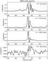 |
Fig. A.2 As in Fig. A.1, but at the peak position of MM1b. |
| In the text | |
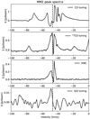 |
Fig. A.3 As in Fig. A.1, but at the peak position of MM2. |
| In the text | |
|
Fig. B.1 Schematic of the parameters for a generalised, non-bicone, outflow model used to limit the possible inclination angles for outflows A and B. |
| In the text | |
Current usage metrics show cumulative count of Article Views (full-text article views including HTML views, PDF and ePub downloads, according to the available data) and Abstracts Views on Vision4Press platform.
Data correspond to usage on the plateform after 2015. The current usage metrics is available 48-96 hours after online publication and is updated daily on week days.
Initial download of the metrics may take a while.