| Issue |
A&A
Volume 642, October 2020
|
|
|---|---|---|
| Article Number | A158 | |
| Number of page(s) | 23 | |
| Section | Cosmology (including clusters of galaxies) | |
| DOI | https://doi.org/10.1051/0004-6361/202038505 | |
| Published online | 15 October 2020 | |
Testing gravity using galaxy-galaxy lensing and clustering amplitudes in KiDS-1000, BOSS, and 2dFLenS
1
Centre for Astrophysics & Supercomputing, Swinburne University of Technology, PO Box 218, Hawthorn, VIC 3122, Australia
e-mail: This email address is being protected from spambots. You need JavaScript enabled to view it.
2
Kavli Institute for Particle Astrophysics & Cosmology, Stanford University, PO Box 2450, Stanford, CA 94305, USA
3
Institute for Astronomy, University of Edinburgh, Royal Observatory, Blackford Hill, Edinburgh EH9 3HJ, UK
4
Center for Theoretical Physics, Polish Academy of Sciences, al. Lotników 32/46, 02-668 Warsaw, Poland
5
Ruhr-University Bochum, Astronomical Institute, German Centre for Cosmological Lensing, Universitätsstr. 150, 44801 Bochum, Germany
6
Argelander-Institut für Astronomie, Auf dem Hügel 71, 53121 Bonn, Germany
7
Department of Physics and Astronomy, University College London, Gower Street, London WC1E 6BT, UK
8
Department of Physics, University of Oxford, Denys Wilkinson Building, Keble Road, Oxford OX1 3RH, UK
9
Department of Astrophysical Sciences, Princeton University, 4 Ivy Lane, Princeton, NJ 08544, USA
10
Leiden Observatory, Leiden University, PO Box 9513, 2300 RA Leiden, The Netherlands
11
Research School of Astronomy and Astrophysics, Australian National University, Canberra, ACT 2611, Australia
12
Korea Astronomy and Space Science Institute, 776 Daedeokdae-ro, Yuseong-gu, Daejeon 34055, Republic of Korea
13
Shanghai Astronomical Observatory (SHAO), Nandan Road 80, Shanghai 200030, PR China
14
University of Chinese Academy of Sciences, Beijing 100049, PR China
Received:
27
May
2020
Accepted:
11
August
2020
Abstract
The physics of gravity on cosmological scales affects both the rate of assembly of large-scale structure and the gravitational lensing of background light through this cosmic web. By comparing the amplitude of these different observational signatures, we can construct tests that can distinguish general relativity from its potential modifications. We used the latest weak gravitational lensing dataset from the Kilo-Degree Survey, KiDS-1000, in conjunction with overlapping galaxy spectroscopic redshift surveys, BOSS and 2dFLenS, to perform the most precise existing amplitude-ratio test. We measured the associated EG statistic with 15 − 20% errors in five Δz = 0.1 tomographic redshift bins in the range 0.2 < z < 0.7 on projected scales up to 100 h−1 Mpc. The scale-independence and redshift-dependence of these measurements are consistent with the theoretical expectation of general relativity in a Universe with matter density Ωm = 0.27 ± 0.04. We demonstrate that our results are robust against different analysis choices, including schemes for correcting the effects of source photometric redshift errors, and we compare the performance of angular and projected galaxy-galaxy lensing statistics.
Key words: dark energy / large-scale structure of Universe / gravitational lensing: weak / surveys
© ESO 2020
1. Introduction
A central goal of modern cosmology is to discover whether the dark energy that appears to fill the Universe is associated with its matter-energy content, laws of gravity, or some alternative physics. A compelling means of distinguishing between these scenarios is to analyse the different observational signatures that are present in the clumpy, inhomogeneous Universe, which powerfully complements measurements of the expansion history of the smooth, homogeneous Universe (e.g. Linder 2005; Wang 2008; Guzzo et al. 2008; Weinberg et al. 2013; Huterer et al. 2015).
Two important observational probes of the inhomogeneous Universe are the peculiar velocities induced in galaxies by the gravitational collapse of large-scale structure, which are statistically imprinted in galaxy redshift surveys as redshift-space distortions (e.g. Hamilton 1998; Scoccimarro 2004; Song & Percival 2009), and the gravitational lensing of light by the cosmic web, which may be measured using cosmic shear surveys (e.g. Bartelmann & Schneider 2001; Kilbinger 2015; Mandelbaum 2018). These probes are complementary because they allow for the differentiation between the two space-time metric potentials which govern the motion of non-relativistic particles, such as galaxy tracers, and the gravitational deflection of light. The difference or “gravitational slip” between these potentials is predicted to be zero in general relativity, but it may be significant in modified gravity scenarios (e.g. Uzan & Bernardeau 2001; Zhang et al. 2007; Jain & Khoury 2010; Bertschinger 2011; Clifton et al. 2012).
Recent advances in weak gravitational lensing datasets, including the Kilo-Degree Survey (KiDS, Hildebrandt et al. 2020), the Dark Energy Survey (DES, Abbott et al. 2018) and the Subaru Hyper Suprime-Cam Survey (HSC, Hikage et al. 2019), have led to dramatic improvements in the quality of these observational tests. Gravitational lensing now permits the accurate determination of, and combinations of, important cosmological parameters such as the matter density of the Universe and normalisation of the matter power spectrum, and thereby detailed comparisons with other cosmological probes such as galaxy clustering (Alam et al. 2017a) and the cosmic microwave background radiation (Planck Collaboration VI 2020). Some of these comparisons have yielded intriguing evidence of “tension” on both small and large scales (e.g. Joudaki et al. 2017; Leauthaud et al. 2017; Lange et al. 2019; Hildebrandt et al. 2020; Asgari et al. 2020a), which are currently unresolved.
In this paper we perform a new study regarding this question using the latest weak gravitational lensing dataset from the Kilo-Degree Survey, KiDS-1000 (Kuijken et al. 2019), in conjunction with overlapping galaxy spectroscopic redshift survey data from the Baryon Oscillation Spectroscopic Survey (BOSS, Reid et al. 2016) and the 2-degree Field Lensing Survey (2dFLenS, Blake et al. 2016a). In particular, we focus on a simple implementation of the lensing-clustering test which compares the amplitude of gravitational lensing around foreground galaxies (commonly known as galaxy-galaxy lensing), tracing low-redshift overdensities, with the amplitude of galaxy velocities induced by these overdensities and measured by redshift-space distortions, which constitutes an amplitude-ratio test. This diagnostic was first proposed by Zhang et al. (2007) as the EG statistic and implemented in its current form by Reyes et al. (2010) using data from the Sloan Digital Sky Survey. These measurements have subsequently been refined by a series of studies (Blake et al. 2016b; Pullen et al. 2016; Alam et al. 2017b; de la Torre et al. 2017; Amon et al. 2018; Singh et al. 2019; Jullo et al. 2019) which have used new datasets to increase the accuracy of the amplitude-ratio determination, albeit showing some evidence of internal disagreement.
The availability of the KiDS-1000 dataset and associated calibration samples has allowed us to perform the most accurate existing amplitude-ratio test, on projected scales up to 100 h−1 Mpc, including rigorous systematic-error control. As part of this analysis, we use these datasets and representative simulations to study the efficacy of different corrections for the effects of source photometric redshift errors, comparing different galaxy-galaxy lensing estimators and the relative performance of angular and projected statistics. Our analysis sets the stage for future per-cent level implementations of these tests using new datasets from the Dark Energy Spectroscopic Instrument (DESI, DESI Collaboration 2016), the 4-metre Multi-Object Spectrograph Telescope (4MOST, de Jong et al. 2019), the Rubin Observatory Legacy Survey of Space and Time (LSST, Ivezić et al. 2019), and the Euclid satellite (Laureijs et al. 2011).
This paper is structured as follows: in Sect. 2 we review the theoretical correlations between weak lensing and overdensity observables, on which galaxy-galaxy lensing studies are based. In Sect. 3 we summarise the angular and projected galaxy-galaxy lensing estimators derived from these correlations, with particular attention to the effect of source photometric redshift errors. In Sect. 4 we introduce the amplitude-ratio test between galaxy-galaxy lensing and clustering observables, constructed from annular differential surface density statistics, and in Sect. 5 we derive the analytical covariances of these estimators in the Gaussian approximation, including the effects of the survey window function. We introduce the KiDS-1000 weak lensing and overlapping Luminous Red Galaxy (LRG) spectroscopic datasets in Sect. 6. We create representative survey mock catalogues in Sect. 7, which we use to verify our cosmological analysis in Sect. 8. Finally, we describe the results of our cosmological tests applied to the KiDS-LRG datasets in Sect. 9. We summarise our investigation in Sect. 10.
2. Theory
In this section we briefly review the theoretical expressions for the auto- and cross-correlations between weak gravitational lensing and galaxy overdensity observables, which form the basis of galaxy-galaxy lensing studies.
2.1. Lensing convergence and tangential shear
The observable effects of weak gravitational lensing, on a source located at co-moving co-ordinate χs in sky direction  , can be expressed in terms of the lensing convergence κ (for reviews, see Bartelmann & Schneider 2001; Kilbinger 2015; Mandelbaum 2018). The convergence is a weighted integral over co-moving distance χ of the matter overdensity δm along the line-of-sight, which we can write as
 (1)
(1)
assuming (throughout this paper) a spatially-flat Universe, where Ωm is the matter density as a fraction of the critical density, H0 is the Hubble parameter, c is the speed of light, and a = 1/(1 + z) is the cosmic scale factor at redshift z. We can conveniently write Eq. (1) in terms of the critical surface mass density at a lens plane at co-moving distance χl,
 (2)
(2)
where G is the gravitational constant, and χs > χl. Hence,
 (3)
(3)
where  is the mean matter density1.
Suppose that the overdensity is associated with an isolated lens galaxy at distance χl in an otherwise homogeneous Universe. In this case, Eq. (3) may be written in the form
 (4)
(4)
Equation (4) motivates that the weak lensing observable can be related to the projected mass density around the lens, Σ = ∫ρm dχ, where  . The convergence may be written in terms of this quantity as
 (5)
(5)
where  represents the average background, emphasising that gravitational lensing traces the increment between the mass density and the background.
The average tangential shear γt at angular separation θ from an axisymmetric lens is related to the convergence as
 (6)
(6)
where  is the mean convergence within separation θ. At the location of the lens, angular separations are related to projected separations as R = χ(zl) θ. Defining the differential projected surface mass density around the lens as a function of projected separation,
 (7)
(7)
where,
 (8)
(8)
we find that for a single source-lens pair at distances χl and χs (omitting the angled brackets),
 (9)
(9)
2.2. Galaxy-convergence cross-correlation
For an ensemble of sources with distance probability distribution ps(χ) (normalised such that ∫ps(χ) dχ = 1), the total convergence in a given sky direction is
 (10)
(10)
where,
 (11)
(11)
with the lower limit of the integral applying because  for χs < χl. We consider forming the angular cross-correlation function of this convergence field with the projected number overdensity of an ensemble of lenses with distance probability distribution pl(χ),
 (12)
(12)
The galaxy-convergence cross-correlation function at angular separation θ is,
 (13)
(13)
Expressing the overdensity fields in terms of their Fourier components we find, after some algebra,
 (14)
(14)
where ℓ is a 2D Fourier wavevector, and the corresponding angular cross-power spectrum Cgκ(ℓ) is given by (Guzik & Seljak 2001; Hu & Jain 2004; Joachimi & Bridle 2010),
 (15)
(15)
where Pgm(k, χ) is the 3D galaxy-matter cross-power spectrum at wavenumber k and distance χ. Taking the azimuthal average of Eq. (14) over all directions θ, the complex exponential integrates to a Bessel function of the first kind, J0(x), such that,
 (16)
(16)
Using Eq. (6) and Bessel function identities, we can then obtain an expression for the statistical average tangential shear around an ensemble of lenses,
 (17)
(17)
Likewise, we can generalise Eq. (9) to apply to broad source and lens distributions:
 (18)
(18)
Comparing the formulations of Eqs. (17) and (18) allows us to demonstrate that,
![Mathematical equation: $$ \begin{aligned} \Sigma (R) = \overline{\rho _{\mathrm{m} }} \int _{-\infty }^\infty \mathrm{d}\Pi \, \left[ 1 + \xi _{\mathrm{gm} }(R,\Pi ) \right] , \end{aligned} $$](/articles/aa/full_html/2020/10/aa38505-20/aa38505-20-eq25.gif) (19)
(19)
in terms of the 3D galaxy-matter cross-correlation function ξgm(R, Π) at projected separation R and line-of-sight separation Π, where the constant term “1+” cancels out in the evaluation of the observable ΔΣ. After some algebra we find,
 (20)
(20)
where,
![Mathematical equation: $$ \begin{aligned} W(r,R) = \frac{4r^2}{R^2} - \left[ \frac{4r \sqrt{r^2-R^2}}{R^2} + \frac{2r}{\sqrt{r^2 - R^2}} \right] \, H(r-R) , \end{aligned} $$](/articles/aa/full_html/2020/10/aa38505-20/aa38505-20-eq27.gif) (21)
(21)
where H(x) = 0 if x < 0 and H(x) = 1 if x > 0 is the Heaviside step function. The relations in this section make the approximations of using the Limber equation (Limber 1953) and neglecting additional effects such as cosmic magnification (Unruh et al. 2020) and intrinsic alignments (Joachimi et al. 2015).
2.3. Auto-correlation functions
In order to determine the analytical covariance in Sect. 5, we also need expressions for the auto-correlation functions of the convergence,  , and the galaxy overdensity,
  . Given two source populations with distance probability distributions ps, 1(χ) and ps, 2(χ), and associated integrated critical density functions
  and
and  , the angular power spectrum of the convergence is given by,
 (22)
(22)
where Pmm(k, χ) is the 3D (non-linear) matter power spectrum at wavenumber k and distance χ. Likewise, for two projected galaxy overdensity fields with distance probability distributions pl, 1(χ) and pl, 2(χ), the angular power spectrum is,
 (23)
(23)
where Pgg(k, χ) is the 3D galaxy power spectrum.
2.4. Bias model
We computed the linear matter power spectrum PL(k) in our models using the CAMB software package (Lewis et al. 2000), and evaluated the non-linear matter power spectrum Pmm(k) including the “halofit” corrections (Smith et al. 2003; Takahashi et al. 2012, we define the fiducial cosmological parameters used for the simulation and data analysis in subsequent sections). We adopted a model for the non-linear galaxy-galaxy and galaxy-matter 2-point functions, appearing in Eqs. (15) and (23), following Baldauf et al. (2010) and Mandelbaum et al. (2013). This model assumes a local, non-linear galaxy bias relation via a Taylor expansion of the galaxy density field in terms of the matter overdensity,  , defining a linear bias parameter bL and non-linear bias parameter bNL. The auto- and cross-correlation statistics in this model can be written in the form (McDonald 2006; Smith et al. 2009),
 (24)
(24)
where ξmm is the correlation function corresponding to Pmm(k), and ξA and ξB are obtained by computing the Fourier transforms of,
 (25)
(25)
which depend on the mode-coupling kernel in standard perturbation theory,
 (26)
(26)
We evaluated these integrals using the FAST software package (McEwen et al. 2016) and note that  , where ξL is the correlation function corresponding to PL(k). This model is only expected to be valid on scales exceeding the virial radius of dark matter haloes, since it does not address halo exclusion, the distribution of galaxies within haloes, or other forms of stochastic or non-local effects (Asgari et al. 2020b). However, this 2-parameter bias model is adequate for our large-scale analysis, which we verify using representative mock catalogues in Sect. 8.
3. Estimators
In this section we specify estimators that may be used to measure γt(θ) and ΔΣ(R) from ensembles of sources and lenses, and discuss how estimates of ΔΣ(R) are affected by uncertainties in source distances.
3.1. Average tangential shear γt(θ)
We can estimate the average tangential shear of a set of sources (s) around lenses (l) by evaluating the following expression (Mandelbaum et al. 2006), which also utilises an unclustered random lens catalogue (r) with the same selection function as the lenses:
 (27)
(27)
The sums in Eq. (27) are taken over pairs of sources and lenses with angular separations within a bin around θ, wi are weights applied to the different samples (normalised such that ∑lwl = ∑rwr), and et indicates the tangential ellipticity of the source, projected onto an axis normal to the line joining the source and lens (or random lens).
Equation (27) involves the random lens catalogue in two places. First, the tangential shear of sources around random lenses is subtracted from the data signal. The subtracted term has an expectation value of zero, but significantly decreases the variance of the estimator at large separations (Singh et al. 2017). Second, the estimator is normalised by a sum over pairs of sources and random lenses, rather than data lenses. This ensures that the estimator is unbiased: the alternative estimator,  , is biased by any source-lens clustering (if the angular cross-correlation function ωls(θ)≠0), which would modify the denominator of the expression but not the numerator. The magnitude of this effect is sometimes known as the “boost” factor (Sheldon et al. 2004),
 (28)
(28)
where the sums are again taken over source-lens pairs with angular separations within a given bin. We note that ⟨B(θ)⟩ = 1 + ωls(θ) for unity weights.
3.2. Projected mass density ΔΣ(R)
Assuming the source and lens distances are known, each source-lens pair may be used to estimate the projected mass density around the lenses by inverting Eq. (9):
 (29)
(29)
For an ensemble of sources and lenses, the mean projected mass density may then be estimated by an expression analogous to Eq. (27) (Singh et al. 2017),
 (30)
(30)
where we have allowed for an additional pair weight between sources and lenses, wls, and random lenses, wrs. Assuming a constant shape noise in et, the noise in the estimate of ΔΣ(R) = et Σc from each source-lens pair is proportional to Σc, hence the optimal inverse-variance weight is  , and the weighted estimator may be written,
 (31)
(31)
3.3. Photo-z dilution correction for ΔΣ(R)
The difficulty faced when determining ΔΣ is that source distances are typically only accessible through photometric redshifts and may contain significant errors, leading to a bias in the estimate through incorrect scaling factors Σc (we assume in this discussion that spectroscopic lens distances are available). For example, sources may apparently lie behind lenses according to their photometric redshift, whilst in fact being positioned in front of the lenses and contributing no galaxy-galaxy lensing signal, creating a downward bias in the measurement.
For a single source-lens pair, the estimated value of Σc for the pair based on the source photometric redshift, Σc, lp, may differ from its true value based on the source spectroscopic redshift, Σc, ls,
 (32)
(32)
Combining many source-lens pairs allowing for a pair weight wls we find,
 (33)
(33)
Using the optimal weight  this expression may be written,
 (34)
(34)
The estimated value of ΔΣ hence contains a multiplicative bias,  where,
 (35)
(35)
This multiplicative correction factor may be estimated at each lens redshift from a representative subset of sources with complete spectroscopic and photometric redshift information, by evaluating the sums in the numerator and denominator of Eq. (35) (Nakajima et al. 2012).
An alternative formulation of the photo-z dilution correction may be derived from the statistical distance distribution of the sources. Provided that the lens distribution is sufficiently narrow, Eq. (18) indicates that an unbiased estimate of ΔΣ from each lens-source pair is,
![Mathematical equation: $$ \begin{aligned} \hat{\Delta \Sigma }(R) = e_{\mathrm{t} }(R/\chi _{\mathrm{l} }) \, \left[ \overline{\Sigma _{\mathrm{c} }^{-1}}(\chi _{\mathrm{l} }) \right]^{-1} , \end{aligned} $$](/articles/aa/full_html/2020/10/aa38505-20/aa38505-20-eq52.gif) (36)
(36)
where  is evaluated from Eq. (11) using the source distribution ps(χ). This motivates an alternative estimator mirroring Eq. (31) (Sheldon et al. 2004; Miyatake et al. 2015; Blake et al. 2016b),
 (37)
(37)
The accuracy of these potential photo-z dilution corrections must be assessed via simulations, which we consider in Sect. 8. We trialled both point-based and distribution-based correction methods in our analysis.
4. Amplitude-ratio test
In this section we construct test statistics which utilise the relative amplitudes of galaxy clustering and galaxy-galaxy lensing to test cosmological models. We first define the input statistics for these tests.
4.1. Projected clustering wp(R)
The amplitude of galaxy-galaxy lensing is sensitive to the distribution of matter around lens galaxies, projected along the line-of-sight. We can obtain an analogous projected quantity for lens galaxy clustering by integrating the 3D galaxy auto-correlation function, ξgg along the line-of-sight,
 (38)
(38)
where Π is the line-of-sight separation. This formulation has the additional feature of reducing sensitivity of the clustering statistics to redshift-space distortions, which modulate the apparent radial separations Π between galaxy pairs.
We can estimate wp(R) for a galaxy sample by measuring the galaxy correlation function in (R, Π) separation bins, and summing over the Π direction in the range 0 < Π < Πmax:
 (39)
(39)
4.2. The Upsilon statistics, Υgm(R) and Υgg(R)
Equation (7) demonstrates that the amplitude of ΔΣ(R) around lens galaxies depends on the surface density of matter across a range of smaller scales from zero to R, and hence on the galaxy-matter cross-correlation coefficient at these scales. Given that this cross-correlation is a complex function which is difficult to model from first principles, it is beneficial to reduce this sensitivity to small-scale information using the annular differential surface density statistic (Reyes et al. 2010; Baldauf et al. 2010; Mandelbaum et al. 2013),
 (40)
(40)
which is defined such that Υgm = 0 at some small-scale limit R = R0, chosen to be large enough to reduce the main systematic effects (typically, R0 is somewhat larger than the size scale of dark matter haloes). In this sense, the cumulative effect from the cross-correlation function at scales R < R0 is cancelled, although it is not the case that this small-scale suppression translates to Fourier space (Baldauf et al. 2010; Asgari et al. 2020b; Park et al. 2020). In any case, the efficacy of these statistics and choice of the R0 value must be validated using simulations, as we consider below.
The corresponding quantity suppressing the small-scale contribution to the galaxy auto-correlations is (Reyes et al. 2010),
![Mathematical equation: $$ \begin{aligned}&\Upsilon _{\mathrm{gg} }(R,R_0) = \rho _{\mathrm{c} } \nonumber \\&\left[ \frac{2}{R^2} \int _{R_0}^R \mathrm{d}R\prime \, R\prime \, w_{\mathrm{p} }(R\prime ) - w_{\mathrm{p} }(R) + \frac{R_0^2}{R^2} \, w_{\mathrm{p} }(R_0) \right] , \end{aligned} $$](/articles/aa/full_html/2020/10/aa38505-20/aa38505-20-eq58.gif) (41)
(41)
where ρc is the critical matter density. We note that if wp is defined as a step-wise function in bins Ri (with bin limits Ri, min and Ri, max) then Eq. (41) may be written in the useful form,
 (42)
(42)
where (k, j) are the bins containing (R, R0), and
 (43)
(43)
For convenience we chose R0 to coincide with the centre of a separation bin, such that we could use the direct measurements of ΔΣ(R0) and wp(R0) in Eqs. (40) and (41) without interpolation between bins (we will show below that our results are not sensitive to the choice of R0).
4.3. The EG test statistic
The relative amplitudes of weak gravitational lensing and the rate of assembly of large-scale structure depend on the “gravitational slip” or difference between the two space-time metric potentials. This signature is absent in general relativity but may be significant in modified gravity scenarios (Uzan & Bernardeau 2001; Zhang et al. 2007; Jain & Khoury 2010; Bertschinger 2011; Clifton et al. 2012).
Zhang et al. (2007) proposed that these amplitudes might be compared by connecting the velocity field and lensing signal generated by a given set of matter overdensities, probed via redshift-space distortions and galaxy-galaxy lensing, respectively. Reyes et al. (2010) implemented this consistency test by constructing the statistic,
 (44)
(44)
where β = f/bL is the redshift-space distortion parameter which governs the observed dependence of the strength of galaxy clustering on the angle to the line-of-sight, in terms of the linear growth rate of a perturbation, f = dlnδ/dlna. Equation (44) is independent of the linear galaxy bias bL and the amplitude of matter clustering σ8, given that β ∝ 1/bL,  and
and  . The prediction of linear perturbation theory for general relativity in a Λ cold dark matter (CDM) Universe is a scale-independent value EG(z) = Ωm(z = 0)/f(z), although see Leonard et al. (2015) for a detailed discussion of this approxmation.
5. Covariance of estimators
In this section we present analytical formulations in the Gaussian approximation for the covariance of estimates of γt(θ) and ΔΣ(R), and model how this covariance is modulated by the presence of a survey mask (that is, by edge effects). Our covariance determination hence neglects non-Gaussian and super-sample variance components. This is a reasonable approximation in the context of the current analysis as these terms are subdominant (we refer the reader to Joachimi et al., in prep. for more details on the relative amplitude of the different covariance terms in the context of KiDS-1000).
5.1. Covariance of average tangential shear
In Appendix A we derive the covariance of γt averaged within angular bins θm and θn:
![Mathematical equation: $$ \begin{aligned} \mathrm{Cov} [\gamma _{\mathrm{t} }^{ij}(\theta _m),\gamma _{\mathrm{t} }^{kl}(\theta _n)] = \frac{1}{\Omega } \int \frac{\mathrm{d}\ell \, \ell }{2\mathrm \pi } \, \sigma ^2(\ell ) \, \overline{J_{2,m}}(\ell ) \, \overline{J_{2,n}}(\ell ) , \end{aligned} $$](/articles/aa/full_html/2020/10/aa38505-20/aa38505-20-eq64.gif) (45)
(45)
where  denotes the average tangential shear of source sample j around lens sample i, Ω is the total survey angular area in steradians, and
  , where the integral is between the bin limits θ1 and θ2 and Ωn is angular area of bin n (i.e. the area of the annulus between the bin limits). The variance σ2(ℓ) is given by the expression for Gaussian random fields (e.g. Hu & Jain 2004; Bernstein 2009; Joachimi & Bridle 2010; Krause & Eifler 2017; Euclid Collaboration 2020),
![Mathematical equation: $$ \begin{aligned} \sigma ^2(\ell ) = C_{\rm g\kappa }^{il}(\ell ) \, C_{\rm g\kappa }^{kj}(\ell ) + \left[ C_{\rm \kappa \kappa }^{jl}(\ell ) + N_{\rm \kappa \kappa }^j \delta ^{\mathrm{K} }_{jl} \right] \, \left[ C_{\mathrm{gg} }^{ik}(\ell ) + N_{\mathrm{gg} }^i \delta ^{\mathrm{K} }_{ik} \right] , \end{aligned} $$](/articles/aa/full_html/2020/10/aa38505-20/aa38505-20-eq67.gif) (46)
(46)
where  is the Kronecker delta. The angular auto- and cross-power spectra appearing in Eq. (46) may be evaluated using the expressions in Sect. 2, and the noise terms are
  and
and  , where σe is the shape noise and
  and
and  are the angular lens and source densities of sample i in units of per steradian.
5.2. Covariance of projected mass density
The covariance of ΔΣ may be deduced from the covariance of γt using  , and by scaling angular separations to projected separations at an effective lens distance χl using θ = R/χl (Singh et al. 2017; Dvornik et al. 2018; Shirasaki & Takada 2018). We can map multipoles ℓ to the projected wavevector k = ℓ/χl such that,
![Mathematical equation: $$ \begin{aligned} \mathrm{Cov} [\Delta \Sigma ^{ij}(R), \Delta \Sigma ^{kl}(R\prime )] = \frac{1}{\Omega } \int \frac{\mathrm{d}k \, k}{2\mathrm \pi } \, \sigma ^2(k) \, \overline{J_2}(k R) \, \overline{J_2}(k R\prime ) , \end{aligned} $$](/articles/aa/full_html/2020/10/aa38505-20/aa38505-20-eq74.gif) (47)
(47)
where we now express the variance in terms of projected power spectra,
![Mathematical equation: $$ \begin{aligned} \sigma ^2(k) = P^{il}_{\rm g\kappa }(k) \, P^{kj}_{\rm g\kappa }(k) + \left[ P^{jl}_{\rm \kappa \kappa }(k) + N^j_{\rm \kappa \kappa } \delta ^{\mathrm{K} }_{jl} \right] \left[ P^{ik}_{\mathrm{gg} }(k) + N^i_{\mathrm{gg} } \delta ^{\mathrm{K} }_{ik} \right] . \end{aligned} $$](/articles/aa/full_html/2020/10/aa38505-20/aa38505-20-eq75.gif) (48)
(48)
The power spectra are given by the following relations:
![Mathematical equation: $$ \begin{aligned} P_{\rm g\kappa }(k) = \frac{\chi _{\mathrm{l} }^2 \, C_{\rm g\kappa }(k\chi _{\mathrm{l} })}{\left[\overline{\Sigma _{\mathrm{c} }^{-1}}(\chi _{\mathrm{l} })\right]^2} \approx \overline{\rho _{\mathrm{m} }} \int \mathrm{d}\chi \, p_{\mathrm{l} }(\chi ) \, P_{\mathrm{gm} }(k,\chi ) , \end{aligned} $$](/articles/aa/full_html/2020/10/aa38505-20/aa38505-20-eq76.gif) (49)
(49)
![Mathematical equation: $$ \begin{aligned}&P_{\rm \kappa \kappa }(k) = \chi _{\mathrm{l} }^2 \, C_{\rm \kappa \kappa }(k\chi _{\mathrm{l} }) \nonumber \\&= \chi _{\mathrm{l} }^2 \, \overline{\rho _{\mathrm{m} }}^2 \int \mathrm{d}\chi \, \left[ \frac{\overline{\Sigma _{\mathrm{c} ,1}^{-1}}(\chi ) \, \overline{\Sigma _{\mathrm{c} ,2}^{-1}}(\chi )}{\overline{\Sigma _{\mathrm{c} ,1}^{-1}}(\chi _{\mathrm{l} }) \, \overline{\Sigma _{\mathrm{c} ,2}^{-1}}(\chi _{\mathrm{l} })} \right] \left( \frac{\chi _{\mathrm{l} }^2}{\chi ^2} \right) \, P_{\mathrm{mm} } \left( \frac{k \, \chi _{\mathrm{l} }}{\chi },\chi \right) , \end{aligned} $$](/articles/aa/full_html/2020/10/aa38505-20/aa38505-20-eq77.gif) (50)
(50)
 (51)
(51)
and the noise terms are,
![Mathematical equation: $$ \begin{aligned} N_{\rm \kappa \kappa } = \frac{\sigma _{\mathrm{e} }^2 \, \chi _{\mathrm{l} }^2}{\overline{n}_{\mathrm{s} } \, \left[ \overline{\Sigma _{\mathrm{c} }^{-1}}(\chi _{\mathrm{l} }) \right]^2} , \; \; \; N_{\mathrm{gg} } = \frac{\chi _{\mathrm{l} }^2}{\overline{n}_{\mathrm{l} }} . \end{aligned} $$](/articles/aa/full_html/2020/10/aa38505-20/aa38505-20-eq79.gif) (52)
(52)
5.3. Covariance of remaining statistics
The expression for the analytical covariance of wp(R) may be derived as (see also, Singh et al. 2017),
![Mathematical equation: $$ \begin{aligned} \mathrm{Cov} [w_{\mathrm{p} }&(R), w_{\mathrm{p} }(R\prime )] = \nonumber \\&\frac{2 L_\parallel \Pi _{\mathrm{max} }}{\Omega } \int \frac{\mathrm{d}k \, k}{2\mathrm \pi } \, \sigma ^2(k) \, J_0(k R) \, J_0(k R\prime ) , \end{aligned} $$](/articles/aa/full_html/2020/10/aa38505-20/aa38505-20-eq80.gif) (53)
(53)
where L∥ is the total co-moving depth of the lens redshift slice and the expression for the variance is,
![Mathematical equation: $$ \begin{aligned} \sigma ^2(k) = \left[ P_{\mathrm{gg} }(k) + N_{\mathrm{gg} } \right]^2 , \end{aligned} $$](/articles/aa/full_html/2020/10/aa38505-20/aa38505-20-eq81.gif) (54)
(54)
where Pgg(k) and Ngg are the 2D projected power spectra and noise as defined in Sect. 5.2.
We determined the analytical covariance of Υgm(R, R0) from the covariance of ΔΣ(R):
![Mathematical equation: $$ \begin{aligned} \mathrm{Cov} [\Upsilon _{\mathrm{gm} }&(R,R_0) , \Upsilon _{\mathrm{gm} }(R\prime ,R_0)] = \mathrm{Cov} [\Delta \Sigma (R) , \Delta \Sigma (R\prime )] \nonumber \\&- \frac{R_0^2}{R^{\prime 2}} \mathrm{Cov} [\Delta \Sigma (R) , \Delta \Sigma (R_0) ] - \frac{R_0^2}{R^2} \mathrm{Cov} [\Delta \Sigma (R\prime ), \Delta \Sigma (R_0) ]\nonumber \\&+ \frac{R_0^4}{R^2 R^{\prime 2}} \mathrm{Var} [\Delta \Sigma (R_0)] . \end{aligned} $$](/articles/aa/full_html/2020/10/aa38505-20/aa38505-20-eq82.gif) (55)
(55)
For the case of Υgg(R, R0), we propagated the covariance using Eq. (42):
![Mathematical equation: $$ \begin{aligned} \mathrm{Cov} [\Upsilon _{\mathrm{gg} }(R,R_0) , \Upsilon _{\mathrm{gg} }(R\prime ,R_0)]&=\frac{\rho _{\mathrm{c} }^2}{R^2 \, R^{\prime 2}}\sum _i \sum _j \nonumber \\&\quad \times C_i \, C_j \, \mathrm{Cov} [w_{\mathrm{p} }(R_i) , w_{\mathrm{p} }(R_j)] . \end{aligned} $$](/articles/aa/full_html/2020/10/aa38505-20/aa38505-20-eq83.gif) (56)
(56)
We evaluated the covariance of the EG statistic, where required, by assuming small fluctuations in the variables in Eq. (44) with respect to their mean, neglecting any correlations between the measurements:
![Mathematical equation: $$ \begin{aligned} \frac{\mathrm{Cov} [E_{\mathrm{G} }(R) \, E_{\mathrm{G} }(R\prime )]}{E_{\mathrm{G} }(R) \, E_{\mathrm{G} }(R\prime )}&= \frac{\mathrm{Cov} [\Upsilon _{\mathrm{gm} }(R,R_0),\Upsilon _{\mathrm{gm} }(R\prime ,R_0)]}{\Upsilon _{\mathrm{gm} }(R,R_0) \, \Upsilon _{\mathrm{gm} }(R\prime ,R_0)} \nonumber \\&\quad + \frac{\mathrm{Cov} [\Upsilon _{\mathrm{gg} }(R,R_0), \Upsilon _{\mathrm{gg} }(R\prime ,R_0)]}{\Upsilon _{\mathrm{gg} }(R,R_0) \, \Upsilon _{\mathrm{gg} }(R\prime ,R_0)} + \frac{\sigma _\beta ^2}{\beta ^2} , \end{aligned} $$](/articles/aa/full_html/2020/10/aa38505-20/aa38505-20-eq84.gif) (57)
(57)
where σβ is the error in the measurement of β. This neglect of correlations is an approximation, justified in the case of our dataset by the fact that the sky area used for the galaxy clustering measurement is substantially different to the sub-sample used for galaxy-galaxy lensing (see Joachimi et al., in prep. for a detailed justification of this approximation), and that the projected lens clustering measurement (Υgg) is largely insensitive to redshift-space distortions (β) owing to the projection over the line-of-sight separations. We note that in our fiducial fitting approach, we determined the scale-independent statistic ⟨EG⟩ through direct fits to Υgm and Υgg as discussed in Sect. 9, without requiring the covariance of EG(R).
5.4. Modification of noise term
We can replace the noise terms in Sects. 5.1 and 5.2 with a more accurate computation using the survey source and lens distributions. Neglecting the random lens term (which is not important on the small scales for which the noise term is significant), we find that the variance associated with the γt estimator in Eq. (27) is (e.g. Miyatake et al. 2019),
![Mathematical equation: $$ \begin{aligned} \mathrm{Var} [\gamma _{\mathrm{t} }(\theta )] = \frac{\sum \limits _{\mathrm{ls} } w_{\mathrm{l} }^2 \, w_{\mathrm{s} }^2 \, \sigma _{\mathrm{e} }^2}{\left( \sum \limits _{\mathrm{rs} } w_{\mathrm{r} } \, w_{\mathrm{s} } \right)^2} . \end{aligned} $$](/articles/aa/full_html/2020/10/aa38505-20/aa38505-20-eq85.gif) (58)
(58)
Likewise, the variance associated with the ΔΣ estimator in Eq. (30) is,
![Mathematical equation: $$ \begin{aligned} \mathrm{Var} [\Delta \Sigma (R)] = \frac{\sum \limits _{\mathrm{ls} } w_{\mathrm{l} }^2 \, w_{\mathrm{s} }^2 \, w_{\mathrm{ls} }^2 \, \sigma _{\mathrm{e} }^2 \left( \Sigma _{\mathrm{c,ls} } \right)^2}{\left( \sum \limits _{\mathrm{rs} } w_{\mathrm{r} } \, w_{\mathrm{s} } \, w_{\mathrm{rs} } \right)^2} . \end{aligned} $$](/articles/aa/full_html/2020/10/aa38505-20/aa38505-20-eq86.gif) (59)
(59)
We adopted these noise terms in our covariance model.
5.5. Modification for survey window
Equations (45) and (47) for the analytical covariance are modified by the survey window function. We can intuitively understand the need for this modification by considering that, whilst Fourier transforms assume periodic boundary conditions, the boundaries of the survey restrict the number of source-lens pairs on scales that are a significant fraction of the survey dimensions.
In Appendix B we derive how the covariance of a cross-correlation function ξ(r) between two Gaussian fields is modified by the window function of the fields, W1(x) and W2(x) (see also, Beutler et al. 2017). We find,
![Mathematical equation: $$ \begin{aligned} \mathrm{Cov} [\xi (r),\xi (s)]&\approx \frac{A_3(r,s)}{A_2(r) \, A_2(s)} \frac{1}{2\mathrm \pi } \int \mathrm{d}k \, k \,\nonumber \\&\quad \times \left[ P_{11}(k) \, P_{22}(k) + P^2_{12}(k) \right] \, J_0(kr) \, J_0(ks) , \end{aligned} $$](/articles/aa/full_html/2020/10/aa38505-20/aa38505-20-eq87.gif) (60)
(60)
where P11, P22 and P12 are the auto- and cross-power spectra of the fields and the pre-factors are given by,
 (61)
(61)
where the integrals over r and s are performed within the separation bin, and we have written A12(x, r) = W1(x) W2(x + r). We hence approximated the dependence of the covariance on the survey window by replacing the survey area in Eqs. (45) and (47) by the expression A2(r) A2(s)/A3(r, s).
We calculated the terms A2 and A3 using the mean and covariance of the pair count RsRl(r) between random source and lens realisations (Landy & Szalay 1993), which have respective densities  and
and  . The mean pair count in a separation bin at scale r (between r1 and r2), containing bin area
  , is
, is
 (62)
(62)
which allows us to find A2(r), given that the other variables are known. The covariance of the pair count between separation bins r and s is,
![Mathematical equation: $$ \begin{aligned} \mathrm{Cov} [ R_{\mathrm{s} }R_{\mathrm{l} }(r) , R_{\mathrm{s} }R_{\mathrm{l} }(s) ]&= \overline{n}_{\mathrm{s} } \, \overline{n}_{\mathrm{l} } \, A_{\mathrm{bin} }(r) \nonumber \\&\times \left[ A_2(r) \, \delta ^K_{rs} + \left( \overline{n}_{\mathrm{s} } + \overline{n}_{\mathrm{l} } \right) A_{\mathrm{bin} }(s) \, A_3(r,s) \right] , \end{aligned} $$](/articles/aa/full_html/2020/10/aa38505-20/aa38505-20-eq93.gif) (63)
(63)
which allows us to determine A3(r, s). For all the source-lens configurations and separation bins considered in this study, we find that the area correction factor differs from 1.0 by less than 10%.
5.6. Propagation of errors in multiplicative corrections
Galaxy-galaxy lensing measurements are subject to multiplicative correction factors arising from shape measurement calibration (see Sect. 6.1) and, in the case of ΔΣ, owing to photometric redshift dilution (see Sect. 3.3). We propagated the uncertainties in these correction factors, which are correlated between different source and lens samples, into the analytical covariance of the measurements. Taking ΔΣ as an example and writing a general amplitude correction factor as α, the relation between the corrected and analytical statistics (denoted by the superscripts ‘corr’ and ‘ana’, respectively) is,
 (64)
(64)
which is normalised such that  , where i denotes the lens sample, j the source sample and k the separation bin. We hence find,
![Mathematical equation: $$ \begin{aligned} \mathrm{Cov} [ \Delta \Sigma ^{\mathrm{corr} }_{ijk} , \Delta \Sigma ^{\mathrm{corr} }_{lmn} ]&= \mathrm{Cov} [ \Delta \Sigma ^{\mathrm{ana} }_{ijk} , \Delta \Sigma ^{\mathrm{ana} }_{lmn} ] \left( 1 + C_{ij,lm} \right) \nonumber \\&+ \langle \Delta \Sigma ^{\mathrm{ana} }_{ijk} \rangle \langle \Delta \Sigma ^{\mathrm{ana} }_{lmn} \rangle \, C_{ij,lm} , \end{aligned} $$](/articles/aa/full_html/2020/10/aa38505-20/aa38505-20-eq96.gif) (65)
(65)
where,
![Mathematical equation: $$ \begin{aligned} C_{ij,lm} = \frac{\langle \alpha _{ij} \alpha _{lm} \rangle - \langle \alpha _{ij} \rangle \langle \alpha _{lm} \rangle }{\langle \alpha _{ij} \rangle \langle \alpha _{lm} \rangle } = \frac{\mathrm{Cov} [ \alpha _{ij}, \alpha _{lm}]}{\langle \alpha _{ij} \rangle \langle \alpha _{lm} \rangle } . \end{aligned} $$](/articles/aa/full_html/2020/10/aa38505-20/aa38505-20-eq97.gif) (66)
(66)
We describe our specific implementation of these equations in the case of the KiDS dataset in Sect. 9.
6. Data
6.1. KiDS-1000
The Kilo-Degree Survey is a large optical wide-field imaging survey optimised for weak gravitational lensing analysis, performed with the OmegaCAM camera on the VLT Survey Telescope at the European Southern Observatory’s Paranal Observatory. The survey covers two regions of sky each containing several hundred square degrees, KiDS-North and KiDS-South, in four filters (u, g, r, i). The companion VISTA-VIKING survey has provided complementary imaging in near-infrared bands (Z, Y, J, H, Ks), resulting in a deep, wide, nine-band imaging dataset.
Our study is based on the fourth public data release of the project, KiDS-1000 (Kuijken et al. 2019), which comprises 1006 deg2 of multi-band data, more than doubling the previously-available coverage. We used an early-science release of the KiDS-1000 shear catalogues, which was created using the exact pipeline version and PSF modelling strategy implemented in Hildebrandt et al. (2017) for the KiDS-450 release. We note that these catalogues have not undergone any rigorous assessment for the presence of cosmic shear systematics, but they are sufficient for the galaxy-galaxy lensing science presented in this paper, as this is less susceptible to systematic errors in the lensing catalogues. The raw pixel data was processed by the THELI and ASTRO_WISE pipelines (Erben et al. 2013; de Jong et al. 2015), and source ellipticities were measured using lensfit (Miller et al. 2013), assigning an optimal weight for each source, and calibrated by a large suite of image simulations (Kannawadi et al. 2019). Photometric redshifts zB were determined from the nine-band imaging for each source using the Bayesian code BPZ (Benítez 2000), calibrated using spectroscopic sub-samples (Hildebrandt et al. 2020), and used to divide the sources into tomographic bins according to the value of zB.
6.2. BOSS
The Baryon Oscillation Spectroscopic Survey (BOSS, Dawson et al. 2013) is the largest existing galaxy redshift survey, which was performed using the Sloan Telescope between 2009 and 2014. BOSS mapped the distribution of 1.5 million Luminous Red Galaxies (LRGs) and quasars across ∼10 000 deg2, inspiring a series of cosmological analyses including the most accurate existing measurements of baryon acoustic oscillations and redshift-space distortions in the galaxy clustering pattern (Alam et al. 2017a). The final (Data Release 12) large-scale structure catalogues are described by Reid et al. (2016); we used the combined LOWZ and CMASS LRG samples in our study2.
6.3. 2dFLenS
The 2-degree Field Lensing Survey (2dFLenS, Blake et al. 2016a) is a galaxy redshift survey performed at the Australian Astronomical Observatory in 2014–2015 using the 2-degree Field spectroscopic instrument, with the goal of extending spectroscopic-redshift coverage of gravitational lensing surveys in the southern sky, particularly the KiDS-South region. The 2dFLenS sample covers an area of 731 deg2 and includes redshifts for 40 531 LRGs in the redshift range z < 0.9, selected by applying BOSS-inspired colour-magnitude cuts to the VST-ATLAS imaging data3. The 2dFLenS dataset has already been utilised in conjunction with the KiDS-450 lensing catalogues to perform a previous implementation of the amplitude-ratio test (Amon et al. 2018), a combined cosmological analysis of cosmic shear tomography, galaxy-galaxy lensing and galaxy multipole power spectra (Joudaki et al. 2018) and to determine photometric redshift calibration by cross-correlation (Johnson et al. 2017; Hildebrandt et al. 2020). In our study we utilised the 2dFLenS LRG sample which overlapped with the KiDS-1000 pointings in the southern region. Figure 1 illustrates the overlaps of the KiDS-1000 source catalogues in the north and south survey regions with the BOSS and 2dFLenS LRG catalogues.
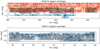 |
Fig. 1. KiDS source and LRG lens catalogues within the KiDS-N region (top panel) and KiDS-S region (bottom panel). The grey squares represent the KiDS-1000 pointings, and the fluctuating background is the gridded number density of 2dFLenS (blue) and BOSS (red) galaxies. The open rectangles outline the footprint of the full KiDS survey, indicating that the LRG overlap will continue to increase as the survey is completed. |
7. Mocks
We used the MICECATv2.0 simulation (Fosalba et al. 2015a,b; Crocce et al. 2015) to produce representative KiDS lensing source catalogues and LRG lens catalogues for testing the estimators, models and covariances described above. The Marenostrum Institut de Ciencias de l’Espai (MICE) catalogues cover an octant of the sky (0 < RA < 90°, 0 < Dec < 90°) for redshift range z < 1.4. We used boundaries at constant RA and Dec to divide this area into 10 sub-samples, each of area 516 deg2. The fiducial set of cosmological parameters for the mock is Ωm = 0.25, h = 0.7, Ωb = 0.044, σ8 = 0.8 and ns = 0.95.
7.1. Mock source catalogue
We constructed the representative mock source catalogue by applying the following steps (see van den Busch et al., in prep. for a full description of the MICE KiDS source mocks). The MICE catalogue is non-uniform across the octant: the region Dec < 30° AND [(RA < 30°) OR (RA > 60°)] has a shallower redshift distribution than the remainder. Firstly, we homogenised the catalogue with the cut des_asahi_full_i_true < 24, such that we could construct mocks using the complete octant. The MICE catalogue shears (γ1, γ2) are defined by the position angle relative to the declination axis. Given the MICE system for mapping 3D positions to (RA, Dec) co-ordinates, the KiDS conventions can be recovered by the following transformations: RA → 90° −RA, γ1 → −γ1 (γ2 is effectively negated twice and therefore unchanged).
We constructed a KiDS-like photometric realisation based on the galaxy sizes and shapes, median KiDS seeing and limiting magnitudes, including photometric noise (see van den Busch et al., in prep.). We ran BPZ photometric redshift estimation (Benítez 2000) on the mock source magnitudes and sizes, assigning zB values for each object. We used a KDTree algorithm to assign weights to the mock sources on the basis of a nearest-neighbour match to the data catalogue in magnitude space, and randomly sub-sampled the catalogue to match the KV450 effective source density. We produced noisy shear components (e1, e2) as e = (γ + n)/(1 + nγ*) (Seitz & Schneider 1997) where γ = γ1 + γ2 i, e = e1 + e2 i and n = n1 + n2 i, where n1 and n2 are drawn from Gaussian distributions with standard deviation σe = 0.288 (Hildebrandt et al. 2020). The redshift distribution estimates of the KiDS data and MICE mock source tomographic samples are displayed in the left panel of Fig. 2, illustrating the reasonable match between the two catalogues.
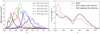 |
Fig. 2. Left panel: redshift distribution estimates of the KiDS source catalogue (solid lines) and MICE mock source catalogue (dashed lines) in the five source tomographic bins split by photometric redshift. Right panel: number density as a function of redshift of the BOSS LRG dataset (black solid line), the MICE mock lens catalogue with the original BOSS colour selection (red dashed line), and the MICE mock lens catalogue with the adjusted BOSS colour selection (blue dotted line). |
7.2. Mock lens catalogue
We constructed the representative mock LRG lens catalogue from the MICE simulation as follows. We used the galaxy magnitudes sdss_g_true, sdss_r_true, sdss_i_true and first applied the MICE evolution correction to these magnitudes as a function of redshift, m → m − 0.8 * [arctan(1.5 * z) − 0.1489] (Crocce et al. 2015). We then constructed the LRG lens catalogues using the BOSS LOWZ and CMASS colour cuts in terms of the variables,
 (67)
(67)
Applying the original BOSS colour-magnitude selection cuts (Eisenstein et al. 2011) to the MICE mock did not reproduce the BOSS redshift distribution (which is unsurprising, since this mock has not been tuned to do so; the BOSS data is also selected from noisy observed magnitudes). Our approach to resolve this issue, following Crocce et al. (2015), was to vary the colour and magnitude selection cuts to minimise the deviation between the mock and data redshift distributions. We applied the following LOWZ selection cuts (where we indicate our changed values in bold font, and the previous values immediately following in square brackets):
![Mathematical equation: $$ \begin{aligned}&16.0 < r < \mathbf 20.0 [19.6] , \nonumber \\&r < \mathbf 13.35 [13.5] + c_\parallel /0.3 , \nonumber \\&|c_\perp | < 0.2 . \end{aligned} $$](/articles/aa/full_html/2020/10/aa38505-20/aa38505-20-eq99.gif) (68)
(68)
We applied the following CMASS selection cuts:
![Mathematical equation: $$ \begin{aligned}&17.5 < i < \mathbf 20.06 [19.9] , \nonumber \\&r - i < 2 , \nonumber \\&d_\perp > 0.55 , \nonumber \\&i < \mathbf 19.98 [19.86] + 1.6 \, (d_\perp -0.8) . \end{aligned} $$](/articles/aa/full_html/2020/10/aa38505-20/aa38505-20-eq100.gif) (69)
(69)
The resulting redshift distributions of the MICE lens mock (original, and after adjustment of the colour selection cuts) and the BOSS data are shown in the right panel of Fig. 2, illustrating that our modified selection produced a much-improved representation of the BOSS dataset. The clustering amplitude of the MICE LRG mock catalogues was consistent with a galaxy bias factor b ≈ 2, although did not precisely match the clustering of the BOSS dataset, since it was not tuned to do so. However, these representative catalogues nonetheless allowed us to test our analysis procedures.
8. Simulation tests
In this section we analyse the representative source and lens catalogues constructed from the MICE mocks described in Sect. 7. Our specific goals are to:
– Test that the non-linear galaxy bias model specified in Sect. 2.4 is adequate for modelling the galaxy-galaxy lensing and clustering statistics across the relevant scales.
– Test that the approaches to the photo-z dilution correction of ΔΣ described in Sect. 3.3 recovered results consistent with those obtained using source spectroscopic redshifts.
– Use the multiple mock realisations and jack-knife techniques to test that the covariance of the estimated statistics is consistent with the analytical Gaussian covariance specified in Sect. 5.
– Test that the EG test statistics constructed from the mock as described in Sect. 4.3 are consistent with the theoretical expectation, and determine the degree to which this result depends on the choice of the small-scale cut-off parameter R0 (see Eq. (40)).
– Test that, given our galaxy bias model, the galaxy-galaxy lensing and clustering statistics may be jointly described by a normalisation parameter σ8 that is consistent with the mock fiducial cosmology, and use this test to assess the relative precision of angular and projected estimators.
Consistent with our subsequent data analysis, we divided the source catalogues into five different tomographic samples by the value of the BPZ photometric redshift, with divisions zB = [0.1, 0.3, 0.5, 0.7, 0.9, 1.2] (following Hildebrandt et al. 2020). We divided the lens catalogue into five slices of spectroscopic redshift zl of width Δzl = 0.1 in the range 0.2 < zl < 0.7. This narrow spectroscopic slicing minimises systematic effects due to redshift evolution across the lens slice (Leauthaud et al. 2017; Singh et al. 2019).
8.1. Measurements
We measured the following three statistics, which form the fundamental set of measurements from which the associated statistics are derived. Firstly, we measured the average tangential shear γt(θ) between all tomographic pairs of source and lens samples, in 15 logarithmically-spaced angular bins in the range 0.005° < θ < 5°, using the estimator of Eq. (27). This measurement is displayed in Fig. 3 as the mean of the 10 individual mock realisations (which each have area 516 deg2), for each of the five source samples against the five lens redshift slices.
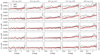 |
Fig. 3. Measurements of the average tangential shear, γt(θ), for the KiDS-LRG dataset (black points) and representative MICE mocks (red points), between all pairs of lens spectroscopic redshift slices (rows) and source tomographic samples split by photometric redshift (columns). The errors are derived from the diagonal elements of the full analytical covariance matrix (where we note that measurements are correlated across scales and samples). The overplotted model is not a fit to this dataset, but rather a prediction based on the galaxy bias parameter fits to the Υgg statistic of each lens redshift slice, which is inaccurate on small scales. The y-values are scaled by a factor of θ (in degrees) for clarity. |
Secondly, we measured the projected mass density ΔΣ(R) between all tomographic pairs of source and lens samples, in 15 logarithmically-spaced projected separation bins in the range 0.1 < R < 100 h−1 Mpc. The mock mean measurement is displayed in Fig. 4 in units of h M⊙ pc−2, for each of the five source samples against the five lens redshift slices. When performing a ΔΣ measurement between source and lens samples we only included individual source-lens galaxy pairs with zB > zl, for which the source photometric redshift lies behind the lens spectroscopic redshift (adopting an alternative cut zB > zl + 0.1 did not change the results significantly). We applied the photo-z dilution correction fbias computed using Eq. (35) based on the point photo-z values, and we study the efficacy of this correction in Sect. 8.2 below.
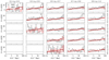 |
Fig. 4. Measurements of the projected mass density, ΔΣ(R), for the KiDS-LRG dataset (black points) and representative MICE mocks (red points), displayed in the same style as Fig. 3. No measurements are possible for the lower left-hand set of panels, owing to the adopted cut in source-lens pairs, zB > zl. The units of ΔΣ are h M⊙ pc−2. |
Thirdly, we measured the projected clustering wp(R) of the lens samples in the same projected separation bins as above, using the estimator of Eq. (39) with Πmax = 100 h−1 Mpc. The mock mean measurement of wp(R) is displayed as the third row of Fig. 5, for each of the five redshift slices. Each of these measurements will be compared with cosmological model predictions as described in the subsections below.
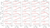 |
Fig. 5. Measurements of a series of galaxy-galaxy lensing and clustering statistics (rows) for each different lens redshift slice (columns) of the MICE mocks. The first row displays the projected mass density ΔΣ(R), where measurements corresponding to the different source tomographic samples have been optimally combined following the procedure described in Appendix C. The second row shows the corresponding measurements of Υgm(R), derived from ΔΣ(R) using Eq. (40) and assuming R0 = 2 h−1 Mpc. The third and fourth rows display the galaxy clustering statistics wp(R) and Υgg(R) for each lens redshift slice, where wp(R) is the projected correlation function measurement, and Υgg(R) is the associated quantity suppressing contributions from small scales, derived using Eq. (41) and again assuming R0 = 2 h−1 Mpc. The fifth row shows the combined-probe statistic EG(R), derived from the Υgm(R) and Υgg(R) measurements using Eq. (44). Errors are displayed using the diagonal elements of the analytical covariance matrix, propagating errors where appropriate. The overplotted models are determined using the galaxy bias factors fitted to the Υgg measurements for each lens redshift slice, and χ2 statistics between the mock mean data and model are displayed in each panel. |
We computed the covariance matrix for each statistic using the analytical Gaussian covariance specified in Sect. 5, where we initially used a fiducial lens linear bias factor bL = 1.8, and iterated this value following a preliminary fit to the projected lens clustering. Figure 6 compares three different determinations of the error in ΔΣ(R) for each individual 516 deg2 realisation of the MICE mocks: using the analytical covariance, using a jack-knife analysis, and derived from the standard deviation of the 10 realisations. For the jack-knife analysis, we divided the sample into 7 × 7 angular regions using constant boundaries in RA and Dec, such that each region contained the same angular area 10.5 deg2. In Fig. 6 we display the comparison as a ratio between the jack-knife or realisations error, and the analytical error.
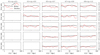 |
Fig. 6. Comparison of different estimates of the error in ΔΣ(R) for individual 516 deg2 realisations of the MICE mocks, between all pairs of lens spectroscopic redshift slices (rows) and source tomographic samples (columns). The black solid line shows the ratio between the error determined by a jack-knife analysis of the data and the error derived from the diagonal elements of the analytical covariance matrix, and the red dashed line is the ratio between the standard deviation across 10 realisations and the analytical error. No measurements are possible for the lower left-hand set of panels, owing to the adopted cut in source-lens pairs, zB > zl. |
We find that in the range R > 1 h−1 Mpc, where the model provides a reasonable description of the measurements, the average (fractional) absolute difference between the analytical and jack-knife errors is 15%, and between the analytical and realisation scatter is 21% (which is the expected level of difference given the error in the variance for 10 realisations). Small differences between these error estimates may arise due to the Gaussian approximation in the analytical covariance, the exact details of the survey modelling, or the scale of the jack-knife regions.
Figure 7 displays the full analytical covariance matrix of ΔΣ(R) – spanning five lens redshift slices, five source tomographic samples and 15 bins of scale – as a correlation matrix with 375 × 375 entries. We note that there are significant off-diagonal correlations between measurements utilising the same lens or source sample, and between different scales. The covariance matrix is reduced in dimension if source-lens sample pairs with zB < zl are excluded, as illustrated by the missing panels in Figs. 4.
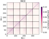 |
Fig. 7. Full analytical covariance matrix Cij of the projected mass density ΔΣ(R) for the MICE mocks, spanning five lens redshift slices, five source tomographic samples and 15 bins of scale – i.e. 375 × 375 entries – ordered where each subsequent bin changes separation, then source sample, then lens sample, such that the vertical and horizontal solid lines demarcate different lens redshift slices. We display the results as a correlation matrix |
We combined the correlated ΔΣ measurements for each individual lens redshift slice, averaging over the five different source tomographic samples, using the procedure described in Appendix C. The resulting combined ΔΣ measurement for each lens redshift sample (again corresponding to a mock mean) is shown as the first row in Fig. 5.
We then used the ΔΣ(R) and wp(R) measurements to infer the Upsilon statistics, Υgm(R, R0) and Υgg(R, R0), using Eqs. (40) and (41) respectively, adopting a fiducial value R0 = 2 h−1 Mpc (we consider the effect of varying this choice below). These measurements are shown in the second and fourth rows of Fig. 5. We determined the covariance of Υgm(R, R0) and Υgg(R, R0) using error propagation following Eqs. (55) and (56), respectively.
Finally, we determined the EG(R) statistic for each lens redshift slice using Eq. (44) where, for the purposes of these tests focussed on galaxy-galaxy lensing, we assumed a fixed input value for the redshift-space distortion parameter β = f(z)/bL(z), where we evaluated f(z) = Ωm(z)0.55 using the fiducial cosmology of the MICE simulation – we note that the exponent 0.55 is an excellent approximation to the solution of the differential growth equation in ΛCDM cosmologies (Linder 2005) – and bL(z) is the best-fitting linear bias parameter to the Υgg measurements for each lens redshift slice z. Hence, systematic errors associated with redshift-space distortions lie beyond the scope of this study, and in our subsequent data analysis we will infer the required β values from existing literature. We propagated errors in EG using Eq. (57) (and assuming no error in β in the case of the mocks). Our EG measurements are shown as the fifth row in Fig. 5.
We generated fiducial cosmological models for these statistics using a non-linear matter power spectrum P(k, z) corresponding to the fiducial cosmological parameters of the MICE simulation listed in Sect. 7. We determined the best-fitting linear and non-linear galaxy bias parameters (bL, bNL) by fitting to the Υgg measurements for each lens redshift slice for scales R > 5 h−1 Mpc, and applied these same bias parameters to the galaxy-galaxy lensing models. The models plotted in Figs. 3, 4 and 5 do not otherwise contain any free parameters. In Fig. 5 we display corresponding χ2 statistics between the models and mock mean data, demonstrating a satisfactory goodness-of-fit in general. We evaluated the χ2 statistics for R > 5 h−1 Mpc for ΔΣ, wp and Υgg, and using all scales for Υgm and EG. We conclude that our lensing and clustering measurements from the MICE mocks generally agree with the underlying ΛCDM cosmology, which we further explore via cosmological parameter fitting in Sect. 8.3.
8.2. Photo-z dilution correction
Within our mock analysis we considered three different implementations of the photo-z dilution correction necessary for the ΔΣ(R) measurements, as described in Sect. 3.3. Firstly, we used the source spectroscopic redshift values (which are available given that this is a simulation) to produce a baseline ΔΣ measurement free of photo-z dilution. Secondly, for our fiducial analysis choice, we used the source photometric redshift point values in the estimator of Eq. (31), adopting a source-lens pair cut zB > zl and correcting for the photo-z dilution using the fbias factor of Eq. (35). We also considered the same case, excluding the fbias correction factor. Thirdly, we used the redshift probability distributions for each source tomographic sample to determine  relative to each lens redshift using Eq. (11), and then estimated ΔΣ using Eq. (37). We refer to this as the P(z) distribution-based method.
The results of these ΔΣ analyses are compared in Fig. 8 for each lens redshift slice, where measurements corresponding to the different source tomographic samples have been optimally combined. We find that, other than in the case where the fbias correction is excluded, both the point-based and distribution-based photo-z dilution corrections produce ΔΣ measurements which are statistically consistent with the baseline measurements using the source spectroscopic redshifts. We further verify in Sect. 8.3 that these analysis choices do not create significant differences in cosmological parameter fits.
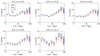 |
Fig. 8. Measurements of the projected mass density ΔΣ for each lens redshift slice of the MICE mocks, where measurements corresponding to the different source tomographic samples have been optimally combined following the procedure described in Appendix C. Results are shown for four cases: using the spectroscopic redshifts of the sources (black points, fiducial measurement with perfect source redshifts), using the photometric redshifts of the sources but without a correction for the photo-z dilution factor fbias (red points, photo-z dilution remains uncorrected), including the dilution correction (green points), and using the redshift probability distribution for each source tomographic slice (blue points). We only include individual source-lens pairs with zB > zl in the measurement. We find that, other than for the case where the fbias correction is excluded, both the point-based and distribution-based photo-z dilution corrections produce ΔΣ measurements which are consistent with those obtained using the source spectroscopic redshifts. |
8.3. Recovery of cosmological parameters
Finally, we verified that our analysis methodology recovered the fiducial cosmological parameters of the MICE simulation within an acceptable statistical accuracy. In this study we focus only on the amplitudes of the clustering and lensing statistics, keeping all other cosmological parameters fixed. In particular we test the recovery of the EG statistics, and the recovery of the σ8 normalisation, marginalising over galaxy bias parameters.
First, we determined a scale-independent EG value (which we denote ⟨EG⟩) for each lens redshift slice from the MICE mock mean statistics displayed in Fig. 5. We considered two approaches to this determination. In one approach, we fitted a constant value to the EG(R) measurements shown in the fifth row of Fig. 5 using the corresponding analytical covariance matrix, that is, varying a vector of five parameters,
![Mathematical equation: $$ \begin{aligned} \boldsymbol{p} = \left[ E_G(z_1) , E_G(z_2) , E_G(z_3) , E_G(z_4) , E_G(z_5) \right] . \end{aligned} $$](/articles/aa/full_html/2020/10/aa38505-20/aa38505-20-eq103.gif) (70)
(70)
This approach has the disadvantage that it is based on the ratio of two noisy quantities Υgm/Υgg, which may result in a biased or non-Gaussian result.
Our second approach avoided this issue by including ⟨EG⟩ as an additional parameter in a joint fit to the Υgm and Υgg statistics for each lens redshift slice, where ⟨EG⟩ changed the amplitude of Υgm relative to Υgg. Specifically, we fitted the model,
 (71)
(71)
in terms of an amplitude parameter AE and galaxy bias parameters bL and bNL, and then determined ⟨EG⟩=AE bL EG, fid for each lens redshift slice, where EG, fid(z) = Ωm/f(z) in terms of the fiducial matter density parameter of the MICE mocks, Ωm, and the theoretical growth rate of structure based on this matter density, f(z). Hence we vary a vector of 15 parameters,
![Mathematical equation: $$ \begin{aligned} \boldsymbol{p} = \left[ A_{\mathrm{E} ,1}, b_{\mathrm{L,1} }, b_{\mathrm{NL,1} }, ..., A_{\mathrm{E} ,5}, b_{\mathrm{L,5} }, b_{\mathrm{NL,5} } \right] . \end{aligned} $$](/articles/aa/full_html/2020/10/aa38505-20/aa38505-20-eq105.gif) (72)
(72)
We note that the bL factor in Eq. (71) for Υgm arises as a consequence of our treatment of β as a fixed input parameter as described in Sect. 8.1, and ensures that AE is constrained only by the relative ratio Υgm/Υgg, and not the absolute amplitude of these functions.
Figure 9 displays the different determinations of ⟨EG⟩ in each lens redshift slice. The left panel compares measurements using the four different treatments of photo-z dilution shown in Fig. 8, confirming that these methods produce consistent EG determinations (other than the case in which fbias is excluded; our fiducial choice is the direct photo-z pair counts with zB > zl). The middle panel compares ⟨EG⟩ fits varying the small-scale parameter R0 (where our fiducial choice is R0 = 2.0 h−1 Mpc, and we also considered choices corresponding to the adjacent separation bins 1.2 and 3.1 h−1 Mpc). The right panel alters the method used to determine ⟨EG⟩, comparing the default choice using the non-linear bias model, a linear model where we fix bNL = 0, and a direct fit to the scale-dependent EG(R) values. Reassuringly, all these methods yielded very similar results.
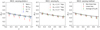 |
Fig. 9. Comparison of the scale-independent values ⟨EG⟩ determined for each lens redshift slice of the MICE mocks, varying the galaxy-galaxy lensing analysis assumptions and methodology. Our fiducial analysis adopted a point-based photo-z correction with zB > zl, R0 = 2.0 h−1 Mpc and a model fitted to (Υgm, Υgg) including non-linear galaxy bias. The left panel compares determinations of ⟨EG⟩ varying the photo-z dilution correction method studying the same four cases described in Fig. 8, the middle panel varies the small-scale parameter R0, and the right panel alters the fitting method to only include linear galaxy bias, and to use a direct fit to the EG(R) values. The model line in each case is the prediction EG(z) = Ωm/f(z), where Ωm is the fiducial matter density parameter for the MICE mocks. |
We compared these determinations to the model prediction EG(z) = Ωm/f(z) shown in Fig. 9. Other than for the case where the fbias correction is excluded, both the point-based and distribution-based photo-z dilution corrections produce determinations of ⟨EG⟩ which recover the fiducial value. This conclusion holds independently of the chosen value of R0, although higher R0 values produce slightly increased error ranges. The different modelling approaches also produce consistent results.
Next, we utilised our mock dataset to perform a fit of the cosmological parameter σ8 to the joint lensing and clustering statistics, marginalising over different bias parameters (bL, bNL) for each redshift slice such that we vary a vector of 11 parameters,
![Mathematical equation: $$ \begin{aligned} \boldsymbol{p} = \left[ \sigma _8, b_{\mathrm{L} ,1}, b_{\mathrm{NL} ,1}, \ldots , b_{\mathrm{L} ,5}, b_{\mathrm{NL} ,5} \right] . \end{aligned} $$](/articles/aa/full_html/2020/10/aa38505-20/aa38505-20-eq106.gif) (73)
(73)
We fixed the remaining cosmological parameters, and performed our parameter fit using a Markov chain Monte Carlo method implemented using the emcee package (Foreman-Mackey et al. 2013). We used wide, uniform priors for each fitted parameter.
As above, we adopted for our fiducial analysis the point photo-z dilution correction using fbias, and we performed fits to the Υgm(R) and Υgg(R) statistics with R0 = 2 h−1 Mpc, considering the same analysis variations as above. Following the scale cuts mentioned above, the data vector contains eight scales for Υgm(R) and seven scales for Υgg(R) for each of the five lens redshift slices, comprising a total of 75 data points.
For this fiducial case, we obtained a measurement σ8 = 0.779 ± 0.019, consistent with the MICE simulation cosmology σ8 = 0.8. The χ2 statistic of the best-fitting model is 69.9 for 64 degrees of freedom (d.o.f.), that is, 75 data points minus the 11 fitted parameters. Figure 10 displays the dependence of the σ8 measurements on the analysis choices. All methodologies using the non-linear bias model recovered the fiducial σ8 value, with the exception of excluding the fbias correction. Adopting a linear bias model instead produced a significantly poorer recovery.
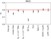 |
Fig. 10. Measurements of the σ8 parameter marginalising over the galaxy bias factors, resulting from fits to the Υgm and Υgg statistics measured for the MICE lens redshift slices. We adopted a 2-parameter galaxy bias model (blin, bNL) for each redshift slice, such that the fit varied 11 parameters in total. The left-hand point resulted from our fiducial analysis choice, assuming R0 = 2.0 h−1 Mpc and a point-based photo-z dilution correction. The second point from the left compares the result of a fit using only the linear galaxy bias parameter (setting bNL = 0). We also show results varying the value of R0 and the photo-z dilution correction. The horizontal red line indicates the MICE simulation fiducial cosmology σ8 = 0.8. |
We also considered fitting to different pairs of lensing-clustering statistics: ΔΣ(R) and wp(R) for R > Rmin = 5 h−1 Mpc, compared to γt(θ) and wp(R), where we applied a minimum-scale cut in θ which matches Rmin in each lens redshift slice. These alternative statistics also successfully recovered the fiducial value of σ8, with errors of 0.018 (for ΔΣ) and 0.022 (for γt). According to this analysis, the projected statistics produced a ∼20% more accurate σ8 value than the angular statistics, in agreement with the results of Shirasaki & Takada (2018).
We conclude this section by noting that the application of our analysis pipeline to the MICE lens and source mocks successfully recovered the fiducial EG and σ8 parameters of the simulation, and is robust against differences in photo-z dilution correction, choice of the small-scale parameter R0, and choice of statistic included in the analysis [γt(θ), ΔΣ(R) or Υgm(R)].
9. Results
9.1. Measurements
We now summarise the galaxy-galaxy lensing and clustering measurements we generated from the KiDS-1000 and overlapping LRG datasets. We cut these catalogues to produce overlapping subsets for our galaxy-galaxy lensing analysis, by only retaining sources and lenses within the set of KiDS pointings which contain BOSS or 2dFLenS galaxies. The resulting KiDS-N sample comprised 15 150 250 KiDS shapes and 47 332 BOSS lenses within 474 KiDS pointings with total unmasked area 366.0 deg2, and the KiDS-S sample consisted of 16 994 252 KiDS shapes and 18 903 2dFLenS lenses within 478 KiDS pointings with total unmasked area 382.1 deg2. We also utilised BOSS and 2dFLenS random catalogues in our analysis, with the same selection cuts and size 50 times bigger than the datasets, sub-sampled from the master random catalogues provided by Reid et al. (2016) and Blake et al. (2016a), respectively.
We split the KiDS-1000 source catalogue into five different tomographic samples by the value of the BPZ photometric redshift, using the same bin divisions zB = [0.1, 0.3, 0.5, 0.7, 0.9, 1.2] adopted in Sect. 8. The effective source density of each tomographic sample is neff = [0.88, 1.33, 2.04, 1.49, 1.26] arcmin−2 (Hildebrandt et al. 2020), estimated using the method of Heymans et al. (2012). We divided the BOSS and 2dFLenS LRG catalogues into five spectroscopic redshift slices of width Δzl = 0.1 in the range 0.2 < zl < 0.7.
We measured the average tangential shear γt(θ) and projected mass density ΔΣ(R) between all pairs of KiDS-1000 tomographic source samples and LRG redshift slices in the north and south regions, using the same estimators and binning as utilised for the MICE mocks in Sect. 8.1 and applying a multiplicative shear bias correction for each tomographic sample (Kannawadi et al. 2019). For the ΔΣ measurement, we again restricted the source-lens pairs such that zB > zl, and (in our fiducial analysis) applied a point-based photo-z dilution correction.
We generated an analytical covariance matrix for each measurement, initially using a fiducial lens linear bias factor bL = 2, and iterating this value following a preliminary fit to the projected lens clustering. We tested that the analytical error determination agreed sufficiently well with a jack-knife error analysis where the regions were defined as the KiDS pointings; the results of this test and the overall analytical covariance are visually similar to their equivalents for the MICE mocks shown in Figs. 6 and 7, and we do not repeat these figures. We used the KV450 spectroscopic calibration sample with DIR weights (Hildebrandt et al. 2020) to estimate the redshift distribution of each tomographic source sample for use in the analytical covariance matrix, in the modelling of γt(θ) and in the distribution-based correction to ΔΣ(R) for photo-z dilution, and to determine the fbias values for the point-based photo-z dilution correction.
We propagated the uncertainties in the multiplicative correction factors due to the shear calibration bias and photometric redshift dilution using the method described in Sect. 5.6. Regarding the multiplicative shear calibration, we followed Hildebrandt et al. (2020) in adopting an error σm = 0.02 that is fully correlated across all samples, such that ![Mathematical equation: $ \mathrm{Cov}[ \alpha_{ij}, \alpha_{lm} ] = \sigma_{\mathrm{m}}^2 $](/articles/aa/full_html/2020/10/aa38505-20/aa38505-20-eq107.gif) in Eq. (66).
in Eq. (66).
The sample variance in the spectroscopic training set can be characterised by an uncertainty in mean spectroscopic redshift which varies for each tomographic sample in the range σz = 0.011 → 0.039 (see Hildebrandt et al. 2020, Table 2). We propagated these errors into the determination of fbias by re-evaluating Eq. (35) shifting all the spectroscopic redshifts by a small amount to determine the derivatives ∂fbias, ij/∂zj, where i denotes the lens sample and j the source sample. Using error propagation, we then scaled the derivatives by the errors σz, j to find the covariance matrix of the uncertainties,
![Mathematical equation: $$ \begin{aligned} \mathrm{Cov} [ f_{\mathrm{bias} ,ij} \, f_{\mathrm{bias} ,lm} ] = \frac{\partial f_{\mathrm{bias} ,ij}}{\partial z_j} \, \frac{\partial f_{\mathrm{bias} ,lm}}{\partial z_m} \, \sigma ^2_{\mathrm{z} ,j} \, \delta ^{\mathrm{K} }_{jm} , \end{aligned} $$](/articles/aa/full_html/2020/10/aa38505-20/aa38505-20-eq108.gif) (74)
(74)
where the final Kronecker delta  indicates that these uncertainities are correlated for different lens samples corresponding to the same source sample, but uncorrelated between source samples (we refer the reader to Joachimi et al., in prep. for further investigation of this point). This uncertainty can be propagated into the analytical covariance matrix using Eqs. (65) and (66) with Cov[αij, αlm]=Cov[fbias, ij fbias, lm].
We used the analytical covariance matrices to combine the separate KiDS-N and KiDS-S measurements into a single joint estimate of the galaxy-galaxy lensing statistics and associated covariance, which we utilised in the remainder of this study (we test the consistency of the individual BOSS and 2dFLenS results in Sect. 9.4). We display the KiDS γt(θ) and ΔΣ(R) galaxy-galaxy lensing measurements in the different tomographic combinations in Figs. 3 and 4. We note again that there are some differences between the galaxy-galaxy lensing signals measured in the mocks and data, given that the mocks have not been tuned to reproduce the BOSS and 2dFLenS clustering properties. These differences are particularly evident on the smallest scales, owing to an inconsistent halo occupation. Our study does not require the mocks to precisely replicate the data in order to test our analysis framework.
We obtained the most accurate measurement of the projected correlation function wp(R) of each lens redshift slice using the full BOSS DR12 dataset, combining the LOWZ and CMASS selections and spanning 9376 deg2 (Reid et al. 2016). We adopted the same spatial separation bins as for the MICE mocks, again assuming Πmax = 100 h−1 Mpc. When analysing the BOSS sample we included completeness weights but excluded “FKP” weights (Feldman et al. 1994), which are designed to optimise the clustering signal-to-noise ratio but may not be appropriate in the case of galaxy-galaxy lensing. The full 2dFLenS dataset is too small to offer a competitive measurement of wp(R), although given that it was selected using BOSS-inspired colour-magnitude cuts, we assumed that the BOSS clustering is representative of the combined LRG sample (and we test this approximation in Sect. 9.4). Since the overlap of the KiDS-N source catalogue and full BOSS sample is small (4% of BOSS), we also assumed that the galaxy-galaxy lensing and clustering measurements are uncorrelated.
We combined the correlated ΔΣ measurements for each lens redshift slice, averaging over the different source samples. Figure 11 displays these measurements, together with the projected clustering wp(R) of the full BOSS sample, the corresponding Υgm(R, R0) and Υgg(R, R0) statistics assuming a fiducial choice R0 = 2 h−1 Mpc (we consider the impact of varying this choice in Sect. 9.4), and the direct EG(R) estimate using Eq. (44).
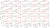 |
Fig. 11. Measurements of a series of galaxy-galaxy lensing and clustering statistics (rows) for each different LRG redshift slice (columns) correlated with the KiDS-1000 source sample, displayed in the same style as Fig. 5. We note that the first and third rows – ΔΣ(R) and wp(R) – represent the original galaxy-galaxy lensing and projected clustering measurements, and the remaining rows – Υgm(R), Υgg(R) and EG(R) – represent statistics derived from these original measurements. |
We generated fiducial cosmological models for these statistics using a non-linear matter power spectrum corresponding to the best-fitting “TTTEEE+lowE+lensing” Planck cosmological parameters (Planck Collaboration VI 2020). When producing the models overplotted in Figs. 3, 4 and 11, we determined best-fitting linear and non-linear galaxy bias parameters by fitting to the Υgg measurements for each lens redshift slice for the separation range R > 5 h−1 Mpc, and applied these same bias parameters to the galaxy-galaxy lensing models. Values of the χ2 statistic for each statistic and lens redshift slice, produced using these models and the analytical covariance, are displayed in each panel of Fig. 11, and indicate that the measurements are consistent with the model.
9.2. Redshift-space distortion inputs
We adopted values of the redshift-space distortion parameters β for the BOSS sample as a function of redshift by interpolating the literature analysis of Zheng et al. (2019), who provide RSD measurements in narrow redshift slices (which also agree with the compilation of results in Alam et al. 2017a). In order to interpolate these measurements to our redshift locations, which slightly differ from the bin centres of Zheng et al. (2019), we created a Gaussian process model for β(z) and its errors, which lie in the range 12 − 20% as a function of redshift, using the sum of a Matern kernel and white noise kernel. We note that the error in β makes up roughly half the variance budget for EG in the lowest lens redshift slice (i.e. increases the total error by  ), but is subdominant for the other redshift slices.
9.3. Amplitude-ratio test EG
We used the KiDS-1000 and LRG clustering and galaxy-galaxy lensing measurements, with the previously-published values of β, to determine a scale-independent value of the amplitude ratio, ⟨EG⟩. We adopted the same fiducial analysis method as for the MICE mocks: we performed a joint fit to the Υgm and Υgg measurements for each redshift slice, varying AE and the bias parameters bL and bNL as in Eq. (71), treating AE as an additional amplitude parameter for Υgm. We then deduced ⟨EG⟩=AE/β, propagating the errors in β assuming all these statistics are independent (please see Sect. 4.3 for a note on this approximation). We used the analytical covariance matrices for these statistics, assumed R0 = 2 h−1 Mpc, and fitted the model to R > 5 h−1 Mpc for Υgg and to all scales for Υgm. We consider the effect of varying these analysis choices in Sect. 9.4. In particular, we note that fitting the directly-determined EG(R) values (shown in the fifth row of Fig. 11) produced results which were entirely consistent with our fiducial analysis.
Our resulting fits for ⟨EG⟩ were [0.43 ± 0.09, 0.45 ± 0.07, 0.33 ± 0.06, 0.38 ± 0.07, 0.34 ± 0.08] for redshifts z = [0.25, 0.35, 0.45, 0.55, 0.65]. The measurements have a small degree of correlation, owing to sharing a common source sample, and the analytical covariance matrix is listed in Table 1. We plot these measurements in Fig. 12, together with a literature compilation (Reyes et al. 2010; Blake et al. 2016b; Pullen et al. 2016; Alam et al. 2017b; de la Torre et al. 2017; Amon et al. 2018; Singh et al. 2019; Jullo et al. 2019). The thickness of the purple shaded stripe in Figs. 12 and 13 illustrates the 68% confidence range of the prediction of the Planck “TTTEEE+lowE+lensing” parameter chain at each redshift, assuming a flat ΛCDM Universe.
Covariance matrix corresponding to our measurements EG = [0.43, 0.45, 0.33, 0.38, 0.34] at z = [0.25, 0.35, 0.45, 0.55, 0.65].
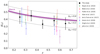 |
Fig. 12. Compilation of measurements of a scale-independent ⟨EG⟩ as a function of redshift. The solid black data points illustrate the results of this study, in five redshift bins. These are compared to literature values from: Reyes et al. (2010) (green), Blake et al. (2016b) (red), Pullen et al. (2016) (magenta), Alam et al. (2017b) (orange), de la Torre et al. (2017) (purple), Amon et al. (2018) (blue), Singh et al. (2019) (cyan) and Jullo et al. (2019) (brown). We note that these previous measurements typically correspond to significantly wider lens redshift ranges than our study, and are also correlated in some cases owing to overlapping datasets. The thickness of the purple shaded stripe illustrates the 68% confidence range of the prediction of the Planck “TTTEEE+lowE+lensing” parameter chain at each redshift assuming a flat ΛCDM Universe, and the dashed lines are the predictions of the model EG(z) = Ωm/f(z) for Ωm = [0.2, 0.3, 0.4]. |
Our measurements provide the best existing determination of the lensing-clustering amplitude ratio (noting that previous measurements displayed in Fig. 12 typically correspond to significantly wider lens redshift ranges than our study), which is consistent with matter density values Ωm ∼ 0.3. Varying the Ωm parameter within a flat ΛCDM cosmological model, assuming EG = Ωm/f = Ωm(0)/Ωm(z)0.55, we find Ωm = 0.27 ± 0.04 (with a minimum χ2 = 1.2 for four d.o.f.). In principle in linear theory, this measurement is insensitive to the other cosmological parameters in a flat ΛCDM scenario. The resulting error in Ωm is, naturally, somewhat larger than that provided by analyses utilising the full shape of the cosmic shear and clustering functions (e.g. Tröster et al. 2020), albeit requiring fewer model assumptions.
We tested for the scale dependence of the EG(R) measurements (in the fifth row of Fig. 11) by jointly fitting an empirical six-parameter model EG(R, zi) = Ai[1+α log10(R)] to all the redshift slices, where α quantifies the fractional variation in EG per decade in projected scale R (in h−1 Mpc) and Ai is a free amplitude for each of the five lens redshift slices. We obtained a 68% confidence region α = 0.17 ± 0.26 (with a minimum χ2 = 35.9 for 34 d.o.f.), which is consistent with no scale dependence, as predicted in the standard gravity scenario. These fits are displayed in Fig. 13.
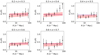 |
Fig. 13. Measurements of the EG(R) statistic for the KiDS-1000 source sample in each LRG lens redshift slice. Errors are derived from the diagonal elements of the analytical covariance matrix, propagating errors where appropriate. The thickness of the purple horizontal stripes illustrates the 68% confidence range of the prediction of the Planck “TTTEEE+lowE+lensing” parameter chain at each redshift assuming a flat ΛCDM Universe, and the red bands illustrate the 68% confidence ranges of a scale-dependent model EG(R, zi) = Ai[1+α log10(R)] discussed in Sect. 9.3. |
9.4. Systematics tests
We now consider the effect on our cosmological fits of varying our fiducial analysis choices. Figure 14 is a compilation of different determinations of ⟨EG⟩ in each lens redshift slice. The upper-left panel compares the fits varying the photo-z dilution correction for ΔΣ between the point-based and distribution-based approaches, and the upper-right panel shows measurements varying the small-scale parameter R0. The lower-left panel considers separate determinations based on the BOSS and 2dFLenS samples (using the BOSS clustering measurements in both cases). The lower-right panel alters the fitting method to only use a linear-bias model (set bNL = 0), and to use a direct fit to the EG(R) measurements presented in the fifth row of Fig. 11, as opposed to our fiducial fits to Υgm and Υgg. In all cases, the systematic variation of the recovered EG values is negligible compared to the statistical errors (noting that the BOSS and 2dFLenS comparison is also subject to sample variance error). We find that varying the photo-z dilution correction, choice of R0 and fitting method produce a systematic variation of 0.08σ, 0.24σ and 0.38σ respectively, when expressed as a fraction of the statistical error σ.
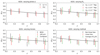 |
Fig. 14. Comparison of the scale-independent values ⟨EG⟩ determined for each LRG redshift slice correlated with the KiDS-1000 source sample, varying the galaxy-galaxy lensing analysis assumptions, sample and methodology. Our fiducial analysis adopted a point-based photo-z correction with zB > zl, R0 = 2.0 h−1 Mpc and a model fitted to (Υgm, Υgg) including non-linear galaxy bias. The upper-left panel compares determinations of ⟨EG⟩ varying the photo-z dilution correction method, the upper-right panel varies the small-scale parameter R0, the lower-left panel varies the lens sample to consider BOSS and 2dFLenS separately, and the lower-right panel alters the fitting method to only include linear galaxy bias, and to use a direct fit to the EG(R) values. The model line in each case is the prediction EG(z) = Ωm/f(z), where Ωm = 0.3. |
10. Summary
We have used the latest weak gravitational lensing data release from the Kilo-Degree Survey, KiDS-1000, together with overlapping galaxy redshift survey data from BOSS and 2dFLenS, to perform cosmological tests associated with the relative amplitude of galaxy-galaxy lensing and galaxy clustering statistics. We quantified our results using the EG(R) statistic, which we were able to measure up to projected separations of 100 h−1 Mpc, recovering a scale-independent value of ⟨EG⟩ with accuracies in the range 15–20% in five lens redshift slices of width Δz = 0.1. The scale-dependence and redshift-dependence of these measurements are consistent with the theoretical expectation of general relativity in a Universe with matter density Ωm ∼ 0.3. The measurements are consistent with a scale-independent model for EG, and constrain allowed variation within 25% (1σ) error per decade in projected scale. Fitting our EG dataset with a flat ΛCDM model, we find Ωm = 0.27 ± 0.04.
We demonstrated that our results are robust against different analysis methodologies. In particular, we showed that:
-
Source photometric redshift errors cause a significant dilution of the inferred projected mass density ΔΣ, by causing unlensed foreground sources to appear in the background of lenses. We demonstrated that this dilution may be corrected either by modifying the estimator for ΔΣ to include the redshift probability distribution of the sources, or by using a source spectroscopic calibration sample to compute the multiplicative bias, producing consistent results. When applied to the mock catalogue, these estimation methods recovered the ΔΣ measurement obtained using source spectroscopic redshifts.
-
A Gaussian analytical covariance for the galaxy-galaxy lensing statistics, with suitable modifications for the survey selection function and small-scale noise terms, predicted errors which agreed within 20% with estimates from a jack-knife procedure and from the variation across mock realisations.
-
Our amplitude-ratio test, based on the annular differential density statistics Υgm and Υgg, is insensitive to the small-scale parameter R0 adopted in these statistics, producing consistent results for choices in the range 1 < R0 < 3 h−1 Mpc. We also obtained consistent results analysing BOSS and 2dFLenS separately.
We performed an additional series of tests jointly fitting an overall amplitude σ8 to the galaxy-galaxy lensing and clustering statistics in our mocks, marginalising over linear and non-linear bias parameters. For our scenario, the projected galaxy-galaxy lensing measurements produced a slightly more accurate determination of σ8 than the angular statistics after matching of scales, although the results are fully consistent.
Our analysis sets the stage for upcoming, increasingly accurate, cosmological tests using amplitude-ratio statistics, as gravitational lensing and galaxy redshift samples continue to grow. These datasets will continue to offer rich possibilities for placing tighter constraints on allowed gravitational physics.
We refer the reader to Dvornik et al. (2018) Appendix C for a full discussion of the different definitions of Σc that have been adopted in the literature.
The BOSS large-scale structure samples are available for download at the link https://data.sdss.org/sas/dr12/boss/lss/.
The 2dFLenS dataset is publicly available at the link http://2dflens.swin.edu.au.
Acknowledgments
We thank the anonymous referee for useful comments on the paper. CB is grateful to Rossana Ruggeri, Alexie Leauthaud, Johannes Lange and Sukhdeep Singh for valuable discussions on galaxy-galaxy lensing measurements. We acknowledge support from: the Australian Research Council Centre of Excellence for All-sky Astrophysics (CAASTRO) through project number CE110001020 (CB, KG); the European Research Council under grant numbers 647112 (MA, BG, CH, TT), 770935 (AD, HH, JLvdB, AHW) and 693024 (SJ); the Polish Ministry of Science and Higher Education through grant DIR/WK/2018/12 and the Polish National Science Center through grant 2018/30/E/ST9/00698 (MB); the Max Planck Society and the Alexander von Humboldt Foundation in the framework of the Max Planck-Humboldt Research Award endowed by the Federal Ministry of Education and Research (CH); Heisenberg grant Hi 1495/5-1 of the Deutsche Forschungsgemeinschaft (HH); the Beecroft Trust (SJ); Vici grant 639.043.512 financed by the Netherlands Organisation for Scientific Research (AK); the Alexander von Humboldt Foundation (KK); the NSFC of China grant 11973070, the Shanghai Committee of Science and Technology grant 19ZR1466600 and Key Research Program of Frontier Sciences grant ZDBS-LY-7013 (HYS); and the European Union’s Horizon 2020 research and innovation programme under the Marie Sklodowska-Curie grant 797794 (TT). The 2dFLenS survey is based on data acquired through the Australian Astronomical Observatory, under program A/2014B/008. It would not have been possible without the dedicated work of the staff of the AAO in the development and support of the 2dF-AAOmega system, and the running of the AAT. Funding for SDSS-III has been provided by the Alfred P. Sloan Foundation, the Participating Institutions, the National Science Foundation, and the U.S. Department of Energy Office of Science. The SDSS-III web site is http://www.sdss3.org/. SDSS-III is managed by the Astrophysical Research Consortium for the Participating Institutions of the SDSS-III Collaboration including the University of Arizona, the Brazilian Participation Group, Brookhaven National Laboratory, Carnegie Mellon University, University of Florida, the French Participation Group, the German Participation Group, Harvard University, the Instituto de Astrofisica de Canarias, the Michigan State/Notre Dame/JINA Participation Group, Johns Hopkins University, Lawrence Berkeley National Laboratory, Max Planck Institute for Astrophysics, Max Planck Institute for Extraterrestrial Physics, New Mexico State University, New York University, Ohio State University, Pennsylvania State University, University of Portsmouth, Princeton University, the Spanish Participation Group, University of Tokyo, University of Utah, Vanderbilt University, University of Virginia, University of Washington, and Yale University. We have used matplotlib (Hunter 2007) for the generation of scientific plots, and this research also made use of astropy, a community-developed core Python package for Astronomy (Astropy Collaboration 2013). Author contributions: all authors contributed to the development and writing of this paper. The authorship list is given in two groups: the lead author (CB), followed by an alphabetical group who have made a significant contribution to either the data products or to the scientific analysis.
References
- Abbott, T. M. C., Abdalla, F. B., Alarcon, A., et al. 2018, Phys. Rev. D, 98, 043526 [Google Scholar]
- Alam, S., Ata, M., Bailey, S., et al. 2017a, MNRAS, 470, 2617 [NASA ADS] [CrossRef] [Google Scholar]
- Alam, S., Miyatake, H., More, S., Ho, S., & Mandelbaum, R. 2017b, MNRAS, 465, 4853 [NASA ADS] [CrossRef] [Google Scholar]
- Amon, A., Blake, C., Heymans, C., et al. 2018, MNRAS, 479, 3422 [NASA ADS] [CrossRef] [Google Scholar]
- Asgari, M., Tröster, T., Heymans, C., et al. 2020a, A&A, 634, A127 [NASA ADS] [CrossRef] [EDP Sciences] [Google Scholar]
- Asgari, M., Friswell, I., Yoon, M., et al. 2020b, ArXiv e-prints [arXiv:2004.07811] [Google Scholar]
- Astropy Collaboration (Robitaille, T. P., et al.) 2013, A&A, 558, A33 [NASA ADS] [CrossRef] [EDP Sciences] [Google Scholar]
- Baldauf, T., Smith, R. E., Seljak, U., & Mand elbaum, R., 2010, Phys. Rev. D, 81, 063531 [NASA ADS] [CrossRef] [Google Scholar]
- Bartelmann, M., & Schneider, P. 2001, Phys. Rev. D, 340, 291 [Google Scholar]
- Benítez, N. 2000, ApJ, 536, 571 [Google Scholar]
- Bernstein, G. M. 2009, ApJ, 695, 652 [NASA ADS] [CrossRef] [Google Scholar]
- Bertschinger, E. 2011, Philos. Trans. R. Soc. London Ser. A, 369, 4947 [Google Scholar]
- Beutler, F., Seo, H.-J., Saito, S., et al. 2017, MNRAS, 466, 2242 [NASA ADS] [CrossRef] [Google Scholar]
- Blake, C., Amon, A., Childress, M., et al. 2016a, MNRAS, 462, 4240 [NASA ADS] [CrossRef] [Google Scholar]
- Blake, C., Joudaki, S., Heymans, C., et al. 2016b, MNRAS, 456, 2806 [NASA ADS] [CrossRef] [Google Scholar]
- Clifton, T., Ferreira, P. G., Padilla, A., & Skordis, C. 2012, Phys. Rep., 513, 1 [NASA ADS] [CrossRef] [MathSciNet] [Google Scholar]
- Crocce, M., Castander, F. J., Gaztañaga, E., Fosalba, P., & Carretero, J. 2015, MNRAS, 453, 1513 [NASA ADS] [CrossRef] [Google Scholar]
- Dawson, K. S., Schlegel, D. J., Ahn, C. P., et al. 2013, AJ, 145, 10 [Google Scholar]
- de Jong, J. T. A., Verdoes Kleijn, G. A., Boxhoorn, D. R., et al. 2015, A&A, 582, A62 [NASA ADS] [CrossRef] [EDP Sciences] [Google Scholar]
- de Jong, R. S., Agertz, O., Berbel, A. A., et al. 2019, The Messenger, 175, 3 [NASA ADS] [Google Scholar]
- de la Torre, S., Jullo, E., Giocoli, C., et al. 2017, A&A, 608, A44 [NASA ADS] [CrossRef] [EDP Sciences] [Google Scholar]
- DESI Collaboration (Aghamousa, A., et al.) 2016, ArXiv e-prints [arXiv:1611.00036] [Google Scholar]
- Dvornik, A., Hoekstra, H., Kuijken, K., et al. 2018, MNRAS, 479, 1240 [NASA ADS] [CrossRef] [Google Scholar]
- Eisenstein, D. J., Weinberg, D. H., Agol, E., et al. 2011, AJ, 142, 72 [Google Scholar]
- Erben, T., Hildebrandt, H., Miller, L., et al. 2013, MNRAS, 433, 2545 [NASA ADS] [CrossRef] [Google Scholar]
- Euclid Collaboration (Blanchard, A., et al.) 2020, A&A, in press, https://doi.org/10.1051/0004-6361/202038071 [Google Scholar]
- Feldman, H. A., Kaiser, N., & Peacock, J. A. 1994, ApJ, 426, 23 [NASA ADS] [CrossRef] [Google Scholar]
- Foreman-Mackey, D., Hogg, D. W., Lang, D., & Goodman, J. 2013, PASP, 125, 306 [CrossRef] [Google Scholar]
- Fosalba, P., Gaztañaga, E., Castander, F. J., & Crocce, M. 2015a, MNRAS, 447, 1319 [NASA ADS] [CrossRef] [Google Scholar]
- Fosalba, P., Crocce, M., Gaztañaga, E., & Castander, F. J. 2015b, MNRAS, 448, 2987 [NASA ADS] [CrossRef] [Google Scholar]
- Guzik, J., & Seljak, U. 2001, MNRAS, 321, 439 [NASA ADS] [CrossRef] [Google Scholar]
- Guzzo, L., Pierleoni, M., Meneux, B., et al. 2008, Nature, 451, 541 [NASA ADS] [CrossRef] [PubMed] [Google Scholar]
- Hamilton, A. J. S. 1998, in Linear Redshift Distortions: a Review, ed. D. Hamilton, Astrophys. Space Sci. Libr., 231, 185 [Google Scholar]
- Heymans, C., Van Waerbeke, L., Miller, L., et al. 2012, MNRAS, 427, 146 [NASA ADS] [CrossRef] [Google Scholar]
- Hikage, C., Oguri, M., Hamana, T., et al. 2019, PASJ, 71, 43 [NASA ADS] [CrossRef] [Google Scholar]
- Hildebrandt, H., Viola, M., Heymans, C., et al. 2017, MNRAS, 465, 1454 [Google Scholar]
- Hildebrandt, H., Köhlinger, F., van den Busch, J. L., et al. 2020, A&A, 633, A69 [NASA ADS] [CrossRef] [EDP Sciences] [Google Scholar]
- Hu, W., & Jain, B. 2004, Phys. Rev. D, 70, 043009 [NASA ADS] [CrossRef] [Google Scholar]
- Hunter, J. D. 2007, Comput. Sci. Eng., 9, 90 [NASA ADS] [CrossRef] [Google Scholar]
- Huterer, D., Kirkby, D., Bean, R., et al. 2015, Astropart. Phys., 63, 23 [Google Scholar]
- Ivezić, Ž., Kahn, S. M., Tyson, J. A., et al. 2019, ApJ, 873, 111 [NASA ADS] [CrossRef] [Google Scholar]
- Jain, B., & Khoury, J. 2010, Ann. Phys., 325, 1479 [NASA ADS] [CrossRef] [Google Scholar]
- Joachimi, B., & Bridle, S. L. 2010, A&A, 523, A1 [NASA ADS] [CrossRef] [EDP Sciences] [Google Scholar]
- Joachimi, B., Cacciato, M., Kitching, T. D., et al. 2015, Space Sci. Rev., 193, 1 [NASA ADS] [CrossRef] [Google Scholar]
- Johnson, A., Blake, C., Amon, A., et al. 2017, MNRAS, 465, 4118 [NASA ADS] [CrossRef] [Google Scholar]
- Joudaki, S., Blake, C., Heymans, C., et al. 2017, MNRAS, 465, 2033 [NASA ADS] [CrossRef] [Google Scholar]
- Joudaki, S., Blake, C., Johnson, A., et al. 2018, MNRAS, 474, 4894 [NASA ADS] [CrossRef] [Google Scholar]
- Jullo, E., de la Torre, S., Cousinou, M. C., et al. 2019, A&A, 627, A137 [CrossRef] [EDP Sciences] [Google Scholar]
- Kannawadi, A., Hoekstra, H., Miller, L., et al. 2019, A&A, 624, A92 [NASA ADS] [CrossRef] [EDP Sciences] [Google Scholar]
- Kilbinger, M. 2015, Rep. Prog. Phys., 78, 086901 [Google Scholar]
- Krause, E., & Eifler, T. 2017, MNRAS, 470, 2100 [Google Scholar]
- Kuijken, K., Heymans, C., Dvornik, A., et al. 2019, A&A, 625, A2 [NASA ADS] [CrossRef] [EDP Sciences] [Google Scholar]
- Landy, S. D., & Szalay, A. S. 1993, ApJ, 412, 64 [NASA ADS] [CrossRef] [Google Scholar]
- Lange, J. U., Yang, X., Guo, H., Luo, W., & van den Bosch, F. C. 2019, MNRAS, 488, 5771 [CrossRef] [Google Scholar]
- Laureijs, R., Amiaux, J., Arduini, S., et al. 2011, ArXiv e-prints [arXiv:1110.3193] [Google Scholar]
- Leauthaud, A., Saito, S., Hilbert, S., et al. 2017, MNRAS, 467, 3024 [NASA ADS] [CrossRef] [Google Scholar]
- Leonard, C. D., Ferreira, P. G., & Heymans, C. 2015, J. Cosmol. Astropart. Phys., 2015, 051 [CrossRef] [Google Scholar]
- Lewis, A., Challinor, A., & Lasenby, A. 2000, ApJ, 538, 473 [Google Scholar]
- Limber, D. N. 1953, ApJ, 117, 134 [NASA ADS] [CrossRef] [Google Scholar]
- Linder, E. V. 2005, Phys. Rev. D, 72, 043529 [NASA ADS] [CrossRef] [MathSciNet] [Google Scholar]
- Mandelbaum, R. 2018, ARA&A, 56, 393 [Google Scholar]
- Mandelbaum, R., Hirata, C. M., Ishak, M., Seljak, U., & Brinkmann, J. 2006, MNRAS, 367, 611 [NASA ADS] [CrossRef] [Google Scholar]
- Mandelbaum, R., Slosar, A., Baldauf, T., et al. 2013, MNRAS, 432, 1544 [NASA ADS] [CrossRef] [Google Scholar]
- McDonald, P. 2006, Phys. Rev. D, 74, 103512 [CrossRef] [Google Scholar]
- McEwen, J. E., Fang, X., Hirata, C. M., & Blazek, J. A. 2016, J. Cosmol. Astropart. Phys., 2016, 015 [CrossRef] [Google Scholar]
- Miller, L., Heymans, C., Kitching, T. D., et al. 2013, MNRAS, 429, 2858 [Google Scholar]
- Miyatake, H., More, S., Mandelbaum, R., et al. 2015, ApJ, 806, 1 [NASA ADS] [CrossRef] [Google Scholar]
- Miyatake, H., Battaglia, N., Hilton, M., et al. 2019, ApJ, 875, 63 [CrossRef] [Google Scholar]
- Nakajima, R., Mandelbaum, R., Seljak, U., et al. 2012, MNRAS, 420, 3240 [NASA ADS] [Google Scholar]
- Park, Y., Rozo, E., & Krause, E. 2020, ArXiv e-prints [arXiv:2004.07504] [Google Scholar]
- Planck Collaboration VI. 2020, A&A, 641, A6 [NASA ADS] [CrossRef] [EDP Sciences] [Google Scholar]
- Pullen, A. R., Alam, S., He, S., & Ho, S. 2016, MNRAS, 460, 4098 [NASA ADS] [CrossRef] [Google Scholar]
- Reid, B., Ho, S., Padmanabhan, N., et al. 2016, MNRAS, 455, 1553 [NASA ADS] [CrossRef] [Google Scholar]
- Reyes, R., Mandelbaum, R., Seljak, U., et al. 2010, Nature, 464, 256 [NASA ADS] [CrossRef] [PubMed] [Google Scholar]
- Scoccimarro, R. 2004, Phys. Rev. D, 70, 083007 [NASA ADS] [CrossRef] [Google Scholar]
- Seitz, C., & Schneider, P. 1997, A&A, 318, 687 [NASA ADS] [Google Scholar]
- Sheldon, E. S., Johnston, D. E., Frieman, J. A., et al. 2004, AJ, 127, 2544 [NASA ADS] [CrossRef] [Google Scholar]
- Shirasaki, M., & Takada, M. 2018, MNRAS, 478, 4277 [CrossRef] [Google Scholar]
- Singh, S., Mandelbaum, R., Seljak, U., Slosar, A., & Vazquez Gonzalez, J. 2017, MNRAS, 471, 3827 [NASA ADS] [CrossRef] [Google Scholar]
- Singh, S., Alam, S., Mandelbaum, R., et al. 2019, MNRAS, 482, 785 [NASA ADS] [CrossRef] [Google Scholar]
- Smith, R. E., Peacock, J. A., Jenkins, A., et al. 2003, MNRAS, 341, 1311 [Google Scholar]
- Smith, R. E., Hernández-Monteagudo, C., & Seljak, U. 2009, Phys. Rev. D, 80, 063528 [NASA ADS] [CrossRef] [Google Scholar]
- Song, Y.-S., & Percival, W. J. 2009, J. Cosmol. Astropart. Phys., 2009, 004 [Google Scholar]
- Takahashi, R., Sato, M., Nishimichi, T., Taruya, A., & Oguri, M. 2012, ApJ, 761, 152 [NASA ADS] [CrossRef] [Google Scholar]
- Tegmark, M., Taylor, A. N., & Heavens, A. F. 1997, ApJ, 480, 22 [NASA ADS] [CrossRef] [Google Scholar]
- Tröster, T., Sánchez, A. G., Asgari, M., et al. 2020, A&A, 633, L10 [CrossRef] [EDP Sciences] [Google Scholar]
- Unruh, S., Schneider, P., Hilbert, S., et al. 2020, A&A, 638, A96 [CrossRef] [EDP Sciences] [Google Scholar]
- Uzan, J.-P., & Bernardeau, F. 2001, Phys. Rev. D, 64, 083004 [NASA ADS] [CrossRef] [Google Scholar]
- Wang, Y. 2008, J. Cosmol. Astropart. Phys., 2008, 021 [NASA ADS] [CrossRef] [Google Scholar]
- Weinberg, D. H., Mortonson, M. J., Eisenstein, D. J., et al. 2013, Phys. Rep., 530, 87 [NASA ADS] [CrossRef] [MathSciNet] [Google Scholar]
- Zhang, P., Liguori, M., Bean, R., & Dodelson, S. 2007, Phys. Rev. Lett., 99, 141302 [NASA ADS] [CrossRef] [PubMed] [Google Scholar]
- Zheng, J., Zhao, G.-B., Li, J., et al. 2019, MNRAS, 484, 442 [CrossRef] [Google Scholar]
Appendix A: Covariance of average tangential shear
We may evaluate the covariance of γt between scales θ and θ′ using Eq. (17),
![Mathematical equation: $$ \begin{aligned} \mathrm{Cov} [\gamma _{\mathrm{t} }^{ij}(\theta ),\gamma _{\mathrm{t} }^{kl}(\theta \prime )]&= \int \frac{\mathrm{d}^2\boldsymbol{\ell }}{(2\mathrm \pi )^2} \int \frac{\mathrm{d}^2\boldsymbol{\ell }\prime }{(2\mathrm \pi )^2} \nonumber \\&\quad \times \mathrm{Cov} [C_{\rm g\kappa }^{ij}(\boldsymbol{\ell }) , C_{\rm g\kappa }^{kl}(\boldsymbol{\ell }\prime )] \, J_2(\ell \theta ) \, J_2(\ell \prime \theta \prime ), \end{aligned} $$](/articles/aa/full_html/2020/10/aa38505-20/aa38505-20-eq111.gif) (A.1)
(A.1)
where  denotes the average tangential shear of source sample j around lens sample i. We adopt an approximation that different multipoles ℓ are uncorrelated such that,
![Mathematical equation: $$ \begin{aligned} \mathrm{Cov} [C_{\rm g\kappa }^{ij}(\boldsymbol{\ell }), C_{\rm g\kappa }^{kl}(\boldsymbol{\ell }\prime )] = \delta _{\mathrm{D} }(\boldsymbol{\ell }- \boldsymbol{\ell }\prime ) \, \sigma ^2(\ell ) , \end{aligned} $$](/articles/aa/full_html/2020/10/aa38505-20/aa38505-20-eq113.gif) (A.2)
(A.2)
where δD is the Dirac delta function, and the variance σ2(ℓ) is given by Eq. (46).
Equation (A.1) becomes, after integrating the delta function  where Ω is the total survey angular area in steradians,
![Mathematical equation: $$ \begin{aligned} \mathrm{Cov} [\gamma _{\mathrm{t} }^{ij}(\theta ),\gamma _{\mathrm{t} }^{kl}(\theta ^{\prime })] = \frac{1}{\Omega } \int \frac{\mathrm{d}\ell \, \ell }{2\mathrm \pi } \, \sigma ^2(\ell ) \, J_2(\ell \theta ) \, J_2(\ell \theta \prime ) . \end{aligned} $$](/articles/aa/full_html/2020/10/aa38505-20/aa38505-20-eq115.gif) (A.3)
(A.3)
If the measurements of γt are averaged within angular bins m and n, where the angular area of the ith bin is Ωi (i.e. the area of the annulus between the bin limits), then the covariance between the bins is,
![Mathematical equation: $$ \begin{aligned} C_{mn}&= \int _m \frac{\mathrm{d}^2\theta }{\Omega _{\mathrm{m} }} \int _n \frac{\mathrm{d}^2\theta \prime }{\Omega _n} \, \mathrm{Cov} [\gamma ^{ij}_{\mathrm{t} }(\theta ),\gamma ^{kl}_{\mathrm{t} }(\theta \prime )] \nonumber \\&= \frac{1}{\Omega } \int \frac{\mathrm{d}\ell \, \ell }{2\mathrm \pi } \, \sigma ^2(\ell ) \, \overline{J_{2,m}}(\ell ) \, \overline{J_{2,n}}(\ell ) , \end{aligned} $$](/articles/aa/full_html/2020/10/aa38505-20/aa38505-20-eq116.gif) (A.4)
(A.4)
where  . We also note that the contribution of any constant term in the covariance σ2(ℓ) = C (such as the noise terms) is,
 (A.5)
(A.5)
using the Bessel function relation  .
.
Appendix B: Modification of covariance for survey window
We derive how the covariance of a cross-correlation function between two Gaussian fields, δ1(x) and δ2(x), is modified by the window function of the fields, W1(x) and W2(x). We adopt the case of a 2D flat sky, where the vector separation r between two points has magnitude r and orientation angle θ. An estimator of the cross-correlation function of the fields at separation r is,
 (B.1)
(B.1)
where  . The expectation value of this expression is,
 (B.2)
(B.2)
where we have introduced the cross-power spectrum P12(k), and the approximation in the third line of Eq. (B.2) ignores the θ dependence of ∫d2x W1(x) W2(x + r).
The covariance of the estimator may be deduced from,
 (B.3)
(B.3)
where we have written A12(x, r) = W1(x) W2(x + r). Expanding this expression using Wick’s theorem for a Gaussian random field, ⟨δ1 δ2 δ3 δ4⟩=⟨δ1 δ2⟩⟨δ3 δ4⟩+⟨δ1 δ3⟩⟨δ2 δ4⟩+⟨δ1 δ4⟩⟨δ2 δ3⟩, we find
![Mathematical equation: $$ \begin{aligned} \mathrm{Cov} [\hat{\xi }(\boldsymbol{r}),\hat{\xi }(\boldsymbol{s})]&= \frac{1}{A_2(r) \, A_2(s)} \int \mathrm{d}^2\boldsymbol{x}\int \mathrm{d}^2\boldsymbol{y}\, \nonumber \\&\quad \times A_{12}(\boldsymbol{x},\boldsymbol{r}) \, A_{12}(\boldsymbol{y},\boldsymbol{s}) \, [ \langle \delta _1(\boldsymbol{x}) \, \delta _1(\boldsymbol{y}) \rangle \langle \delta _2(\boldsymbol{x}+\boldsymbol{r}) \, \delta _2(\boldsymbol{y}+\boldsymbol{s}) \rangle \nonumber \\&\quad + \langle \delta _1(\boldsymbol{x}) \, \delta _2(\boldsymbol{y}+\boldsymbol{s}) \rangle \langle \delta _2(\boldsymbol{x}+\boldsymbol{r}) \, \delta _1(\boldsymbol{y}) \rangle ] . \end{aligned} $$](/articles/aa/full_html/2020/10/aa38505-20/aa38505-20-eq124.gif) (B.4)
(B.4)
Using  , and omitting some algebra, the first term evaluates to,
 (B.5)
(B.5)
and the second term evaluates to,
 (B.6)
(B.6)
The expression for the covariance is then,
![Mathematical equation: $$ \begin{aligned} \mathrm{Cov} [\hat{\xi }(\boldsymbol{r}),\hat{\xi }(\boldsymbol{s})]&= \frac{\int \mathrm{d}^2\boldsymbol{x}\, A_{12}(\boldsymbol{x},\boldsymbol{r}) \, A_{12}(\boldsymbol{x},\boldsymbol{s})}{A_2(r) \, A_2(s)}\nonumber \\&\quad \int \frac{\mathrm{d}^2\boldsymbol{k}}{(2\mathrm \pi )^2} \, \left[ P_{11}(\boldsymbol{k}) \, P_{22}(\boldsymbol{k}) + P^2_{12}(\boldsymbol{k}) \right] \, \mathrm{e} ^{\mathrm{i} \boldsymbol{k}\cdot (\boldsymbol{r}-\boldsymbol{s})} . \end{aligned} $$](/articles/aa/full_html/2020/10/aa38505-20/aa38505-20-eq128.gif) (B.7)
(B.7)
Averaging the estimator over angles we obtain,
![Mathematical equation: $$ \begin{aligned} \mathrm{Cov} [\hat{\xi }(r),\hat{\xi }(s)]&\approx \frac{A_3(r,s)}{A_2(r) \, A_2(s)}\frac{1}{2\mathrm \pi } \int \mathrm{d}k \, k \, \nonumber \\&\quad \times \left[ P_{11}(k) \, P_{22}(k) + P^2_{12}(k) \right] \, J_0(kr) \, J_0(ks) , \end{aligned} $$](/articles/aa/full_html/2020/10/aa38505-20/aa38505-20-eq129.gif) (B.8)
(B.8)
where A3(r, s) = ∫d3r∫d3s∫d2x A12(x, r) A12(x, s).
Appendix C: Combining correlated tomographic slices
In order to reduce the size of a data vector, we can optimally combine separate correlated estimates of a statistic, such as a galaxy-galaxy lensing measurement for a given lens sample against different tomographic source slices. This procedure is an example of data compression (Tegmark et al. 1997).
Suppose we have measured a given statistic at Nr different scales, for Ns source tomographic slices, and we wish to average the statistic over source samples, where the measurements in the different slices are correlated. We’ll arrange these quantities in a data vector x of length NsNr with corresponding covariance matrix C of dimension NsNr × NsNr. The operation to combine the different tomographic slices to a compressed data vector y of length Nr can be written as,
 (C.1)
(C.1)
where w is a weight matrix of dimension NsNr × Nr, and we normalise the weights such that the column corresponding to each scale bin sums to unity. The optimal choice of weight matrix (Tegmark et al. 1997) is,
 (C.2)
(C.2)
where D is a matrix of dimension NsNr × Nr, whose columns consist of NsNr entries for each final scale bin, with value 1 when the entry in x corresponds to the same scale bin, and value 0 otherwise. The resulting covariance matrix of y is,
 (C.3)
(C.3)
which has dimension Nr × Nr.
We found that this data compression scheme is more robust against numerical issues with the matrix inverse (and suffers negligible loss in precision) if we replaced the weight matrix with w = V−1 D, where V is a diagonal matrix just containing the variance of the measurements. In this implementation the weight matrix is slightly suboptimal, but we retained the full covariance matrix in Eq. (C.3) to ensure correct error propagation.
All Tables
Covariance matrix corresponding to our measurements EG = [0.43, 0.45, 0.33, 0.38, 0.34] at z = [0.25, 0.35, 0.45, 0.55, 0.65].
All Figures
|
Fig. 1. KiDS source and LRG lens catalogues within the KiDS-N region (top panel) and KiDS-S region (bottom panel). The grey squares represent the KiDS-1000 pointings, and the fluctuating background is the gridded number density of 2dFLenS (blue) and BOSS (red) galaxies. The open rectangles outline the footprint of the full KiDS survey, indicating that the LRG overlap will continue to increase as the survey is completed. |
| In the text | |
|
Fig. 2. Left panel: redshift distribution estimates of the KiDS source catalogue (solid lines) and MICE mock source catalogue (dashed lines) in the five source tomographic bins split by photometric redshift. Right panel: number density as a function of redshift of the BOSS LRG dataset (black solid line), the MICE mock lens catalogue with the original BOSS colour selection (red dashed line), and the MICE mock lens catalogue with the adjusted BOSS colour selection (blue dotted line). |
| In the text | |
|
Fig. 3. Measurements of the average tangential shear, γt(θ), for the KiDS-LRG dataset (black points) and representative MICE mocks (red points), between all pairs of lens spectroscopic redshift slices (rows) and source tomographic samples split by photometric redshift (columns). The errors are derived from the diagonal elements of the full analytical covariance matrix (where we note that measurements are correlated across scales and samples). The overplotted model is not a fit to this dataset, but rather a prediction based on the galaxy bias parameter fits to the Υgg statistic of each lens redshift slice, which is inaccurate on small scales. The y-values are scaled by a factor of θ (in degrees) for clarity. |
| In the text | |
|
Fig. 4. Measurements of the projected mass density, ΔΣ(R), for the KiDS-LRG dataset (black points) and representative MICE mocks (red points), displayed in the same style as Fig. 3. No measurements are possible for the lower left-hand set of panels, owing to the adopted cut in source-lens pairs, zB > zl. The units of ΔΣ are h M⊙ pc−2. |
| In the text | |
|
Fig. 5. Measurements of a series of galaxy-galaxy lensing and clustering statistics (rows) for each different lens redshift slice (columns) of the MICE mocks. The first row displays the projected mass density ΔΣ(R), where measurements corresponding to the different source tomographic samples have been optimally combined following the procedure described in Appendix C. The second row shows the corresponding measurements of Υgm(R), derived from ΔΣ(R) using Eq. (40) and assuming R0 = 2 h−1 Mpc. The third and fourth rows display the galaxy clustering statistics wp(R) and Υgg(R) for each lens redshift slice, where wp(R) is the projected correlation function measurement, and Υgg(R) is the associated quantity suppressing contributions from small scales, derived using Eq. (41) and again assuming R0 = 2 h−1 Mpc. The fifth row shows the combined-probe statistic EG(R), derived from the Υgm(R) and Υgg(R) measurements using Eq. (44). Errors are displayed using the diagonal elements of the analytical covariance matrix, propagating errors where appropriate. The overplotted models are determined using the galaxy bias factors fitted to the Υgg measurements for each lens redshift slice, and χ2 statistics between the mock mean data and model are displayed in each panel. |
| In the text | |
|
Fig. 6. Comparison of different estimates of the error in ΔΣ(R) for individual 516 deg2 realisations of the MICE mocks, between all pairs of lens spectroscopic redshift slices (rows) and source tomographic samples (columns). The black solid line shows the ratio between the error determined by a jack-knife analysis of the data and the error derived from the diagonal elements of the analytical covariance matrix, and the red dashed line is the ratio between the standard deviation across 10 realisations and the analytical error. No measurements are possible for the lower left-hand set of panels, owing to the adopted cut in source-lens pairs, zB > zl. |
| In the text | |
|
Fig. 7. Full analytical covariance matrix Cij of the projected mass density ΔΣ(R) for the MICE mocks, spanning five lens redshift slices, five source tomographic samples and 15 bins of scale – i.e. 375 × 375 entries – ordered where each subsequent bin changes separation, then source sample, then lens sample, such that the vertical and horizontal solid lines demarcate different lens redshift slices. We display the results as a correlation matrix |
| In the text | |
|
Fig. 8. Measurements of the projected mass density ΔΣ for each lens redshift slice of the MICE mocks, where measurements corresponding to the different source tomographic samples have been optimally combined following the procedure described in Appendix C. Results are shown for four cases: using the spectroscopic redshifts of the sources (black points, fiducial measurement with perfect source redshifts), using the photometric redshifts of the sources but without a correction for the photo-z dilution factor fbias (red points, photo-z dilution remains uncorrected), including the dilution correction (green points), and using the redshift probability distribution for each source tomographic slice (blue points). We only include individual source-lens pairs with zB > zl in the measurement. We find that, other than for the case where the fbias correction is excluded, both the point-based and distribution-based photo-z dilution corrections produce ΔΣ measurements which are consistent with those obtained using the source spectroscopic redshifts. |
| In the text | |
|
Fig. 9. Comparison of the scale-independent values ⟨EG⟩ determined for each lens redshift slice of the MICE mocks, varying the galaxy-galaxy lensing analysis assumptions and methodology. Our fiducial analysis adopted a point-based photo-z correction with zB > zl, R0 = 2.0 h−1 Mpc and a model fitted to (Υgm, Υgg) including non-linear galaxy bias. The left panel compares determinations of ⟨EG⟩ varying the photo-z dilution correction method studying the same four cases described in Fig. 8, the middle panel varies the small-scale parameter R0, and the right panel alters the fitting method to only include linear galaxy bias, and to use a direct fit to the EG(R) values. The model line in each case is the prediction EG(z) = Ωm/f(z), where Ωm is the fiducial matter density parameter for the MICE mocks. |
| In the text | |
|
Fig. 10. Measurements of the σ8 parameter marginalising over the galaxy bias factors, resulting from fits to the Υgm and Υgg statistics measured for the MICE lens redshift slices. We adopted a 2-parameter galaxy bias model (blin, bNL) for each redshift slice, such that the fit varied 11 parameters in total. The left-hand point resulted from our fiducial analysis choice, assuming R0 = 2.0 h−1 Mpc and a point-based photo-z dilution correction. The second point from the left compares the result of a fit using only the linear galaxy bias parameter (setting bNL = 0). We also show results varying the value of R0 and the photo-z dilution correction. The horizontal red line indicates the MICE simulation fiducial cosmology σ8 = 0.8. |
| In the text | |
|
Fig. 11. Measurements of a series of galaxy-galaxy lensing and clustering statistics (rows) for each different LRG redshift slice (columns) correlated with the KiDS-1000 source sample, displayed in the same style as Fig. 5. We note that the first and third rows – ΔΣ(R) and wp(R) – represent the original galaxy-galaxy lensing and projected clustering measurements, and the remaining rows – Υgm(R), Υgg(R) and EG(R) – represent statistics derived from these original measurements. |
| In the text | |
|
Fig. 12. Compilation of measurements of a scale-independent ⟨EG⟩ as a function of redshift. The solid black data points illustrate the results of this study, in five redshift bins. These are compared to literature values from: Reyes et al. (2010) (green), Blake et al. (2016b) (red), Pullen et al. (2016) (magenta), Alam et al. (2017b) (orange), de la Torre et al. (2017) (purple), Amon et al. (2018) (blue), Singh et al. (2019) (cyan) and Jullo et al. (2019) (brown). We note that these previous measurements typically correspond to significantly wider lens redshift ranges than our study, and are also correlated in some cases owing to overlapping datasets. The thickness of the purple shaded stripe illustrates the 68% confidence range of the prediction of the Planck “TTTEEE+lowE+lensing” parameter chain at each redshift assuming a flat ΛCDM Universe, and the dashed lines are the predictions of the model EG(z) = Ωm/f(z) for Ωm = [0.2, 0.3, 0.4]. |
| In the text | |
|
Fig. 13. Measurements of the EG(R) statistic for the KiDS-1000 source sample in each LRG lens redshift slice. Errors are derived from the diagonal elements of the analytical covariance matrix, propagating errors where appropriate. The thickness of the purple horizontal stripes illustrates the 68% confidence range of the prediction of the Planck “TTTEEE+lowE+lensing” parameter chain at each redshift assuming a flat ΛCDM Universe, and the red bands illustrate the 68% confidence ranges of a scale-dependent model EG(R, zi) = Ai[1+α log10(R)] discussed in Sect. 9.3. |
| In the text | |
|
Fig. 14. Comparison of the scale-independent values ⟨EG⟩ determined for each LRG redshift slice correlated with the KiDS-1000 source sample, varying the galaxy-galaxy lensing analysis assumptions, sample and methodology. Our fiducial analysis adopted a point-based photo-z correction with zB > zl, R0 = 2.0 h−1 Mpc and a model fitted to (Υgm, Υgg) including non-linear galaxy bias. The upper-left panel compares determinations of ⟨EG⟩ varying the photo-z dilution correction method, the upper-right panel varies the small-scale parameter R0, the lower-left panel varies the lens sample to consider BOSS and 2dFLenS separately, and the lower-right panel alters the fitting method to only include linear galaxy bias, and to use a direct fit to the EG(R) values. The model line in each case is the prediction EG(z) = Ωm/f(z), where Ωm = 0.3. |
| In the text | |
Current usage metrics show cumulative count of Article Views (full-text article views including HTML views, PDF and ePub downloads, according to the available data) and Abstracts Views on Vision4Press platform.
Data correspond to usage on the plateform after 2015. The current usage metrics is available 48-96 hours after online publication and is updated daily on week days.
Initial download of the metrics may take a while.