| Issue |
A&A
Volume 668, December 2022
|
|
|---|---|---|
| Article Number | A12 | |
| Number of page(s) | 17 | |
| Section | Cosmology (including clusters of galaxies) | |
| DOI | https://doi.org/10.1051/0004-6361/202243758 | |
| Published online | 28 November 2022 | |
Galaxy–galaxy lensing in the VOICE deep survey
1
School of Physics and Astronomy, Sun Yat-sen University Zhuhai Campus, 2 Daxue Road, Tangjia, Zhuhai, Guangdong 519082, PR China
e-mail: napolitano@mail.sysu.edu.cn
2
Shanghai Key Lab for Astrophysics, Shanghai Normal University, Shanghai 200234, PR China
e-mail: fuliping@shnu.edu.cn
3
CAS Key Laboratory for Research in Galaxies and Cosmology, University of Science and Technology of China, Hefei, Anhui 230026, PR China
e-mail: wtluo@ustc.edu.cn
4
Department of Astronomy, School of Physical Sciences, University of Science and Technology of China, Hefei, Anhui 230026, PR China
5
INAF – Osservatorio Astronomico di Padova, Via dell’Osservatorio 5, 35122 Padova, Italy
6
South-Western Institute for Astronomy Research, Yunnan University, Kunming, 650500 Yunnan, PR China
7
Dipartimento di Fisica ‘E. Pancini’, Universita degli Studi Federio II, Napoli 80126, Italy
8
INFN, Sezione di Napoli, Napoli 80126, Italy
9
INAF – Osservatorio Astronomico di Capodimonte, Salita Moiariello 16, Napoli 80131, Italy
10
Inter-University Institute for Data Intensive Astronomy, Department of Astronomy, University of Cape Town, 7701 Rondebosch, Cape Town, South Africa
11
Inter-University Institute for Data Intensive Astronomy, Department of Physics and Astronomy, University of the Western Cape, 7535 Bellville, Cape Town, South Africa
12
INAF – Istituto di Radioastronomia, Via Globetti 101, 40129 Bologna, Italy
Received:
12
April
2022
Accepted:
13
September
2022
The multi-band photometry of the VOICE imaging data, overlapping with 4.9 deg2 of the Chandra Deep Field South (CDFS) area, enables both shape measurement and photometric redshift estimation to be the two essential quantities for weak lensing analysis. The depth of magAB is up to 26.1 (5σ limiting) in r-band. We estimate the excess surface density (ESD; ΔΣ) based on galaxy–galaxy measurements around galaxies at lower redshift (0.10 < zl < 0.35) while we select the background sources as those at higher redshift ranging from 0.3 to 1.5. The foreground galaxies are divided into two major categories according to their colour (blue and red), each of which has been further divided into high- and low-stellar-mass bins. The halo masses of the samples are then estimated by modelling the signals, and the posterior of the parameters are sampled using a Monte Carlo Markov chain process. We compare our results with the existing stellar-to-halo mass relation (SHMR) and find that the blue low-stellar-mass bin (median M* = 108.31 M⊙) deviates from the SHMR relation whereas the other three samples agree well with empirical curves. We interpret this discrepancy as the effect of the low star-formation efficiency of the low-mass blue dwarf galaxy population dominated in the VOICE-CDFS area.
Key words: gravitational lensing: weak / methods: statistical / surveys / galaxies: halos / large-scale structure of Universe / dark matter
© R. Luo et al. 2022
 Open Access article, published by EDP Sciences, under the terms of the Creative Commons Attribution License (https://creativecommons.org/licenses/by/4.0), which permits unrestricted use, distribution, and reproduction in any medium, provided the original work is properly cited.
This article is published in open access under the Subscribe-to-Open model. Subscribe to A&A to support open access publication.
1. Introduction
A major challenge in the study of galaxy formation is to understand the co-evolution processes of gas, stars, and dark matter in galaxies as a function of their properties, such as mass and colour (Wechsler & Tinker 2018). Theoretical studies (see e.g., White & Rees 1978; Fukugita et al. 1998; Faucher-Giguère et al. 2011; Somerville & Davé 2015) suggest that the physical progress of galaxy formation is driven by the properties of their dark matter haloes, in particular their mass. Hydrodynamical simulations have recently reached sufficient accuracy to study the effect of stellar feedback and other strong mechanisms, such as active galactic nucleus (AGN) and supernova (SN) feedback at relatively small scales (Illustris, Vogelsberger et al. 2014; EAGLE, Schaye et al. 2015), also allowing us to study the effect of gas and stellar processes on the final dark matter distribution (White & Rees 1978; Blumenthal et al. 1986; Davé et al. 2012). Ultimately, we expect these simulations to finally bridge baryonic and dark matter properties (Yang et al. 2006) and allow the so-called galaxy–halo connection to be elucidated (Wechsler & Tinker 2018).
Observationally speaking, abundance matching (Conroy & Wechsler 2009; Behroozi et al. 2010; Moster et al. 2013) – such as the relation between the stellar, M*, and dark matter (DM) mass, MDM – in halos, which is obtained by matching the observed galaxy luminosity function and the predicted halo mass function from simulations (see e.g., Tinker et al. 2005; Vale & Ostriker 2006; Conroy et al. 2006), is one of the primary semi-empirical tests of the existence of such a connection. Another popular method is the halo occupation distribution (HOD; Berlind & Weinberg 2002; Kravtsov et al. 2004; Zheng et al. 2005; Zu & Mandelbaum 2016), which populates dark matter haloes with galaxies to reproduce galaxy clustering (Jing et al. 1998; Seljak 2000; Peacock & Smith 2000; Cooray & Sheth 2002) as a function of luminosity over a wide redshift range (Vale & Ostriker 2004; Conroy et al. 2006). Furthermore, there are more complex methods developed with the HOD approach, such as the conditional luminosity function (CLF; Yang et al. 2003) and conditional stellar mass function (CMF; Moster et al. 2010). These methods constitute hybrid approaches based on statistical relations between observed galaxies and simulated halos, and, as such, they are strongly model dependent.
On the other hand, to fully test the theoretical expectation, a direct measurement of both the stellar and the dark component of galaxies is needed in order to construct a M* − MDM relation. One possibility to achieve this is to use dynamical-based methods to obtain the total mass in galaxies (see e.g., Blumenthal et al. 1986; Zaritsky & White 1994; McKay et al. 2002; Prada et al. 2003). Another possibility is provided by gravitational lensing. This is a powerful technique to infer the galaxy masses at different scales. In the case of strong lensing, arcs or multiple images of background ‘source’ galaxies allow us to efficiently constrain the total mass in the central regions of foreground ‘lens’ systems (Kochanek 1995; Treu 2010). In the case of weak lensing (WL), the effect of the weak distortion over a large statistical sample of background galaxies can be used to infer the total mass density out to very large distances for an ensemble of foreground lens systems (Brainerd et al. 1996; Bartelmann & Schneider 2001; Munshi et al. 2008; Hoekstra & Jain 2008). In this latter case, the WL method of the so-called galaxy–galaxy lensing is a tool applied to study the cross-correlation of background galaxies with foreground underlying matter by correlating the distortion of background galaxies to the position of foreground galaxies. We specifically refer to galaxy–galaxy lensing to distinguish it from other forms of WL from a larger distribution of matter in clusters (see e.g., Natarajan & Kneib 1997; Geiger & Schneider 1999) or cosmic scales (see e.g., Mandelbaum et al. 2013; Kwan et al. 2017).
The last few decades have seen great progress in weak gravitational lensing studies from wide-field and deep sky surveys. These surveys have provided high-quality photometric images for the studies of WL, which include galaxy–galaxy lensing, such as the Sloan Digital Sky Survey (SDSS; York et al. 2000; Guzik & Seljak 2002; Cacciato et al. 2009, 2013; Luo et al. 2018), the Canada-France-Hawaii Telescope Lensing Survey (CFHTLenS; Heymans et al. 2012; Kilbinger et al. 2013; Fu et al. 2014; Hudson et al. 2015), Dark Energy Survey (DES; The Dark Energy Survey Collaboration 2005; Dark Energy Survey Collaboration 2016; Clampitt et al. 2017; Abbott et al. 2018), Kilo-Degree Survey (KiDS; Kuijken et al. 2015; Viola et al. 2015; van Uitert et al. 2018; Dvornik et al. 2020), Hyper-Suprime-Cam survey (HSC; Aihara et al. 2018; Wang et al. 2021), and so on. Because of the variety of astrophysical answers that WL can provide about DM, this has become the main science driver for most future large survey projects. Future space-based surveys will be provided by the missions of Euclid (Refregier et al. 2010) and Roman (Spergel et al. 2015), and Chinese Space Station Optical Survey (CSS-OS; Zhan 2011, 2018; Gong et al. 2019). In terms of future ground-based surveys, there is the Legacy Survey of Space and Time (LSST; LSST Science Collaboration 2009) that will be carried out over the following decade.
In this paper, we are focussing on the Chandra Deep Field South (CDFS) region of the VST Optical Imaging of the CDFS and European Large Area ISO Survey South-1 (ES1) Fields survey (VOICE; Vaccari et al. 2016), and we estimate the two-dimensional excess surface density (ESD) of galaxy–galaxy lensing from the measurements of tangential shape signals of sources from the shear catalogue in VOICE-CDFS which are presented in Fu et al. (2018; hereafter F18). We apply a Markov chain Monte Carlo (MCMC) method to build a halo model that can constrain the halo parameters of foreground galaxies, and finally directly derive the relation between the stellar and halo mass for central and satellite galaxies (Yang et al. 2006) in the VOICE-CDFS region.
The structure of this paper is as follows. In Sect. 2, we present the dataset from the VOICE survey. In Sect. 3, we illustrate the shear catalogue from the background source sample and the selection of foreground (lens) samples based on the photometric catalogue of the galaxies in VOICE. In Sect. 4 we introduce the galaxy–galaxy lensing estimator, while in Sect. 5 we present the weak lensing model that we adopt to estimate the halo parameters. The ESD measurements and the model results are presented in Sect. 6, together with a comparison of the ESD results obtained using the DES-Y1 shear catalogue overlapping with VOICE on the CDFS area. In Sect. 7, we finally discuss the results and draw some conclusions.
2. VOICE Survey and shear catalogue
The VOICE Survey is a Guaranteed Time of Observation (GTO) survey carried out with the European Southern Observatory (ESO) VLT Survey Telescope (VST; Capaccioli & Schipani 2011) on Cerro Paranal in Chile. VOICE observations have been carried out from October 2011 to 2015 to obtain deep optical imaging of two patches of the sky, each of about 5 deg2, centred on the CDFS and on the ES1. The two areas are referred to as VOICE-CDFS (RA = 03h32m30s, Dec = −27° 48′30″) and VOICE-ES1 (RA = 00h34m45s, Dec = −43° 28′00″), respectively.
These two areas have been targeted in the past in different projects and in different wavelength ranges, including ultraviolet (UV) from GALEX (Martin et al. 2005), near-infrared (NIR) band from VISTA/VIDEO (Jarvis et al. 2013), mid-infrared (MIR) band from Spitzer-Warm/SERVS (Mauduit et al. 2012), far-infrared (FIR) from Herschel/HerMES (Oliver et al. 2012), infrared (IR) from Spitzer-Cold/SWIRE (Lonsdale et al. 2003), and radio band in ATCA/ATLAS (Franzen et al. 2015). VOICE was designed to provide deep, high-quality observations in ugri bands on VOICE-CDFS field and u-band on VOICE-ES1 field.
In this paper, we use r-band data of the 4.9 deg2 area of VOICE-CDFS. This is composed of four pointings (CDFS-1/2/3/4) observed with the OmegaCAM (Kuijken 2011), which consists of 32 detectors with 2048 × 4096 pixels and a scale of 0.21 arcsec pixels−1. The adopted tiling strategy was the same as that used for weak lensing observations in KiDS (Kuijken et al. 2019). There are more than 100 r-band exposures in each of the four tiles, making this the deepest band available in VOICE. For the four different areas, the cumulative exposure time is in the range of 15.30–20.90 h. Just like in KiDS, the observations consisted in five continuous exposures every epoch by repeating a diagonal pattern to cover the detector gaps between charge-coupled devices (CCDs). The VOICE data we used in the galaxy–galaxy lensing study are based on the shear catalogue from F18, where the galaxy shapes have been measured by LensFit (Miller et al. 2013). The VOICE shear catalogue was derived from the r-band stacked images, as a product of an analysis pipeline including image co-adding, star and bad-pixel masking, object detection, point spread function (PSF) fitting, shape measurements, and so on (see F18).
The final catalogue of objects classified as galaxies is made up of 583 131 objects (see F18 for details). For these galaxies, the measurements of photometric redshifts (photo-z) were based on the data of the optical observations in u, g, r, i from VOICE together with the NIR observations in Z, Y, J, H, Ks from the VIDEO survey (Jarvis et al. 2013), using the BPZ software (Benítez 2011). We refer to this as the photometric catalogue in the following.
Finally, the shear catalogue was obtained using LensFit (Miller et al. 2013) as the shape measurement algorithm for OmegaCAM images. In particular, the weak lensing shear measurements are based on r band images with ≤0.9 arcsec seeing in the VOICE survey.
The shear catalogue of VOICE-CDFS contains the data of 310 985 galaxies corresponding to an effective weighted galaxy number density of about 16.35 gal arcmin−2, which is about twice the density of the KiDS survey. The limiting AB magnitude for a point source in 2 arcsec aperture is 26.1 mag in r-band. We refer the interested reader to F18 for further details about the data reduction and the validation of the shear and photo-z catalogues.
3. Galaxy sample
The photometric galaxy catalogue and the shear catalogue have different purposes. The former provides photometric information about all galaxies identified in the CDFS area in VOICE. These are all galaxies that can be used as potential lenses at different redshifts in our galaxy–galaxy lensing estimates. The photo-z derived from BPZ has accepted systematic errors and F18 show there is good agreement between photo-z with spectroscopic redshift (spec-z) for the matched galaxies. The shear catalogue, instead, is a list of galaxies for which we have been able to measure the apparent distortion due to the weak lensing effect. As such, this is the catalogue where we need to select the background sources in the surrounding area of each foreground lens chosen from the photometric catalogue.
3.1. Photo-z and stellar masses
As discussed in F18, the photo-z estimation in the VOICE study is the peak value of the probability density function, and the photo-z data were derived using the BPZ software. We checked the comparison of the measurements of photo-z with the corresponding spec-z (Vaccari et al. 2010, 2016) for the matched 23 638 galaxies in Fig. 1, and find that it shows a good agreement on the whole. F18 present the median value of the difference between photo-z and spec-z: δz = (Zphot − Zspec)/(1 + Zspec) = 0.008, with median absolute deviation σ = 0.06. For the photometric catalogue and shear catalogue, we consider the uncertainties of sources from BPZ are good enough to support the photo-z used for estimating galaxy–galaxy lensing signals.
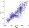 |
Fig. 1. Comparison of photo-z (Zphot) vs. spec-z (Zspec) for the matched galaxies (black points) sample (Fu et al. 2018). The contours present the galaxy number density. The red line is the one-to-one relation. |
Galaxy masses are derived using the standard spectral energy distribution (SED) fitting software, Le-Phare1 (Arnouts et al. 1999; Ilbert et al. 2006). As we want to ultimately study the halo properties of the lens sample, and relate these to their stellar mass properties, we used the photometric galaxy multi-band (optical plus NIR) catalogue to estimate the stellar masses. Here Le-Phare is fed with the full nine-band photometry from the VOICE galaxy catalogue to produce, as output, the best stellar population parameters, including age, metallicity, star formation rate, and stellar mass. The stellar population synthesis (SPS) models (Conroy & Wechsler 2009) we have adopted to match the multi-band photometry are stellar templates from Bruzual & Charlot (2003) with a Chabrier (2003) initial mass function (IMF) and an exponential decaying star formation history.
For the Le-Phare run, we used a broad set of models with different metallicities (0.005 ≤ Z/Z⊙ ≤ 2.5) and ages (age ≤ agemax), with the maximum age, agemax, set by the age of the Universe at the redshift of the galaxy, with a maximum value at z = 0 of 13.5 Gyr. We also considered internal extinction using the Calzetti et al. (1994) models. Finally, to reduce the degeneracies between the redshift and galaxy colours, we fixed the galaxy redshift to the VOICE catalogue photo-z.
3.2. Lens sample
As mentioned in Sect. 3, the lens sample is based on the photometric galaxy catalogue, regardless of whether or not any shear has been measured for them. Among these, we selected galaxies in the range of 0.1 < zl(BPZ) < 0.35 as ‘Full Lens Sample’ (FLS), for which all gri-band magnitudes are available. This sample is made up of 46 188 galaxies, containing positions and photo-z for each of them. The distribution of photo-z of this FLS, shown in Fig. 2, has a median of 0.29 which is the peak value. The choice of this specific redshift range for the FLS is made to maximise the number of foreground galaxies to guarantee a galaxy density that minimises the statistical errors over the two-dimensional lensing signal represented in Sect. 4.2.
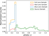 |
Fig. 2. Normalised distribution of photo-z (BPZ) for the galaxies of the Full Lens Sample (orange histogram) and Source Sample (green histogram). The distributions of the Red Lens and Blue Lens samples (red and blue dashed histogram, respectively) are normalised to the FLS. The redshift range of the FLS is 0.1 < zl < 0.35 and that of the Sources Sample is 0.3 < zs < 1.5. |
The mean luminosity of the FLS is Mr ∼ −18.06 with a scatter of σ(Mr)∼1.61 mag, while the averaged logarithmic stellar mass is log M*/M⊙ = 8.56, with a scatter of σ(log M*/M⊙) = 0.96. This rather low mean value and large scatter imply that a large portion of the lens systems have low mass. Indeed, the stellar masses are distributed in the range 106 − 1012 M⊙, meaning that they cover a very wide mass range going from dwarf galaxies to giant ellipticals. As we seek to obtain mean dark halo properties of the lens sample for different populations, which are a strong function of the stellar mass (e.g., Moster et al. 2013), we decided to bin galaxies in stellar mass.
Furthermore, to study the halo properties as a function of galaxy type (e.g., Mandelbaum et al. 2006; Hudson et al. 2015), we roughly separate the passive red galaxies from some active bluer systems, and further bin them in colour. The distribution of galaxy colours as a function of the r-band rest-frame magnitude is shown in Fig. 3. Here we can clearly identify a red sequence at the rest frame [g − i]rest > 0.9, for Mr < −19. We therefore classified FLS into the red and blue lenses by separating the galaxies above and below the dashed line in Fig. 3, respectively, naming these the Red Lens and Blue Lens samples (also referred to as red lenses and blue lenses hereafter). We tried to use other colour classifications of red and blue galaxies, such as [u − g]rest, [g − r]rest (Bell et al. 2003), [u − r]rest (Baldry et al. 2004), but these methods do not clearly demonstrate the obvious bimodal distribution in the colour–magnitude diagram for the FLS as seen in Fig. 3. Figure 2 shows the distributions of the photometric redshifts of the Red and Blue lenses, of which the means are 0.24 and 0.26, respectively.
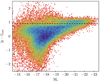 |
Fig. 3. Distribution of colour [g − i] (rest-frame) vs. r-band absolute magnitude for the FLS. The colour coding of the points (from red to blue) represents increasing galaxy number density. The black dashed line is the criterion of [g − i]rest = 0.9 to separate red and blue galaxies. There are two sequences of galaxies in [g − i]rest > 0.9 and [g − i]rest < 0.9 that are considered as the galaxies of Red Lens and Blue Lens, respectively. |
In Fig. 4 we use the colour separation above to display the mass distribution of the two colour classes. This shows a clear bimodal distribution in log M* for the Red and Blue Lens samples. The Red Lens sample contains 5822 galaxies and the Blue Lens sample 40 366 with medians log M*/M⊙ of 9.88 and 8.37, respectively. Looking at the distributions of the stellar masses in Fig. 4, we can see that the most massive bin, that is, log M*/M⊙ > 10.5, is mainly occupied by objects from the Red Lens sample, while in the bin 9.5 < log M*/M⊙ < 10.5 there is a mix of blue and red lenses, although the former are dominant in absolute number. In the lower mass range, 7.0 < log M*/M⊙ < 9.5, the blue lenses reach their peak at log M*/M⊙ ∼ 8.5, while they start to become incomplete at lower masses. There is an insufficient number of red lenses in the same mass bin, 8.5 < log M*/M⊙ < 9.5, to produce a significant lensing signal. Therefore, to obtain a significant colour–mass separation of the FLS, we defined the following samples:
-
Blue Lens-1 and -2: 107.0 < M*/M⊙ < 109.5, 109.5 < M*/M⊙ < 1010.5, respectively;
-
Red Lens-1 and -2: 109.5 < M*/M⊙ < 1010.5, M*/M⊙ > 1010.5, respectively.
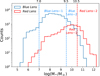 |
Fig. 4. Distribution of logarithmic stellar mass from Blue Lens (blue histogram) and Red Lens (red histogram). The Blue Lens-1 and 2 are from the logarithmic stellar mass bins of [7.0, 9.5] and [9.5, 10.5] in Blue Lens. The Red Lens-1 and 2 are from the logarithmic stellar mass bins of [9.5, 10.5] and > 10.5 in Red Lens. |
In Table 1 we summarise the galaxy number, the median of photo-z and logarithmic stellar mass for the four lens subsamples. Hereafter, we make use of the median values of these parameters to characterise the four lens samples.
Statistics of Red Lens-1 and -2, Blue Lens-1 and -2, and FLS with the mass bin range, numbers, median photo-z, and median logarithmic stellar mass.
3.3. Source sample and lens–source pairs
As a background galaxy sample (the sources), we select galaxies from the shear catalogue of VOICE-CDFS with photo-z in the range of 0.3 < zs(BPZ) < 1.5. The distribution of photo-z is shown in Fig. 2.
The lens–source pairs are then selected using the condition that Δzp = zs − zl > 0.2. This criterion has been adopted to take into account the errors on the photometric redshifts and avoid confusion between background and foreground objects if too close in redshift. According to F18, the typical photo-z errors are ∼0.06 for z < 0.83 and ∼0.1 for z > 0.83. Using Δzp > 0.2 therefore allows us to separate foreground from background with ∼2σ significance.
4. Galaxy–galaxy lensing estimator
4.1. Tangential shear
Galaxy–galaxy lensing signal estimator is based on the measurement of tangential shear γt from background sources around the foreground lenses. As mentioned above, galaxy shapes were measured by F18 using LensFit, where galaxy ellipticities γ1 and γ2 were derived from OmegaCAM images with an accuracy to ≤1%. These measurements are used to estimate the tangential component γt and cross component γ× of shear signals of background sources around a lens galaxy for the jth lens–source pair according to the equations
![$$ \begin{aligned} \left[ \begin{array}{c} \gamma _{t,j} \\ \gamma _{\times ,j}\\ \end{array} \right] =\left[ \begin{array}{cc} -\cos {(2\phi _j)}&-\sin {(2\phi _j)} \\ \sin {(2\phi _j)}&-\cos {(2\phi _j)}\\ \end{array} \right] \left[ \begin{array}{c} \gamma _{1,j} \\ \gamma _{2,j}\\ \end{array} \right], \end{aligned} $$](/articles/aa/full_html/2022/12/aa43758-22/aa43758-22-eq1.gif)
where ϕj is the angle between the separation vector of the jth lens–source pair with the horizontal axis in the Cartesian coordinate system centred on each object of the lens. In weak lensing, the weak distortion of the intrinsic shape due to the warped space-time caused by the lenses of each independent background source is too small to be detected. Hence, in order to detect the shear signals, we need to average over large numbers of lens–source pairs to finally measure, in particular, the tangential component of the shear. This allows us to derive the signal around a lens sample in angular bins θ (Mandelbaum et al. 2005a; Luo et al. 2018),
where  is the responsivity of source galaxies derived by the Eqs. (5)–(7) in Jarvis et al. (2003), and here
  is the weight from LensFit for the jth lens–source pair. This quantity is then used to derive a proxy of the mass density as a function of the angular distance from the common centre of the lens sample adopted to measure it.
4.2. Excess surface density
The ESD (ΔΣ) is defined as the discrepancy between  with
with  , which are the averaged projected surface mass densities inside of radius R and at radius R,

There is a connection between the ESD and the tangential shear from background sources. Indeed, the ΔΣ can be written as (Hudson et al. 2015)
![$$ \begin{aligned} \Delta \Sigma (R; z_{\rm l})&= \Sigma _{\rm crit}(z_{\rm l},z_{\rm s})\overline{\gamma }_{\rm t} (R; z_{\rm l},z_{\rm s})\nonumber \\&= \frac{\Sigma _j[{ w}_j\gamma _{\mathrm{t},j}(R; z_{\rm l},z_{\rm s})/\Sigma ^{-1}_{\mathrm{crit,}j}(z_{\rm l},z_{\rm s})]}{\Sigma _j { w}_j}, \end{aligned} $$](/articles/aa/full_html/2022/12/aa43758-22/aa43758-22-eq8.gif)
where the critical surface density Σcrit is defined as
where Dl, Ds, and Dls are the angular diameter distance of the lens, background source, and that between the two objects, respectively.
In this equation, pairs are weighted by the  , such that we write the weights wj for the jth lens–source pair as
Therefore, Eq. (4) states that we can estimate the ESDs directly from the mean tangential shear signal of sources around the lenses in the different bins of projected separation R. However, we need to correct the shear for possible biases in the shear measurements by LensFit. The shear calibration (Liu et al. 2018) brings a multiplicative, m, and an additive, c, bias into the shear estimation that allow us to convert the observed shear into a ‘true’ signal as
where a presents two components (a = 1, 2) of galaxy ellipticities. This calibration can be applied to our averaged ESD measurement as above to obtain a corrected mean ESD measurement. This is a function of lens redshift and is written as follows:
![$$ \begin{aligned}&\Delta \Sigma ^\mathrm{lens}(R)=\frac{1}{2\overline{\mathcal{R} }}\frac{\Sigma _j { w}_j[-(\gamma _{1,j}-c_{1,j})\cos {2R_j}]\Sigma _{\rm crit}}{\Sigma _j { w}_j (1+m_{1,j})}\nonumber \\&\qquad \qquad \quad +\frac{1}{2\overline{\mathcal{R} }}\frac{\Sigma _j { w}_j[-(\gamma _{2,j}-c_{2,j})\sin {2R_j}]\Sigma _{\rm crit}}{\Sigma _j { w}_j (1+m_{2,j})}, \end{aligned} $$](/articles/aa/full_html/2022/12/aa43758-22/aa43758-22-eq13.gif)
where c1 and c2 are the additive biases and m1 and m2 are the multiplicative biases, obtained as discussed in F18. The estimated values of c1 and c2 are ∼8 × 10⁻⁴ and ∼3 × 10⁻⁵ for γ1 and γ2, respectively (see F18). As these values are ≪1, they have almost no effect on the shear measurements. On the other hand, the multiplicative biases m1 and m2 are quite uniformly distributed in the ranges (−0.494, 0.678) and (−0.362, 0.696), respectively, and they must therefore be taken into account.
Finally, to derive an unbiased ESD estimator, we need to subtract the tangential shear measurements around random points that ought not to have a net lensing signal. This writes as

However, according to the random test in Sect. 6.1, the ESD measurements from tangential shear signals of the random sample, ΔΣrand(R), are generally consistent with zero. Here we would consider the noise ΔΣrand(R) measured from the random lens samples with our source sample as the subtracted one in our final ESD measurements.
4.3. Boost factor
Although we have attempted to avoid overlap between the lens and source pairs by considering a zs − zl separation in photo-z of larger than 0.2 (see Sect. 3.3), there could still be a fraction of background sources that are physically connected to the lenses, causing a scale-dependent bias of lensing signal due to galaxy clustering (Sheldon et al. 2004). To correct for the effect of this correlation between lens and background sources, we apply a multiplicative boost factor B(R). This is defined as the ratio between the weighted number of background galaxies per unit area around the lens and those around random points:
where i, j and k, l denote the sources found around the real lens and the random points, respectively, and wi, j or wk, l are the weight for the pair between each background source with one lens or a random point (Sheldon et al. 2004).
Figure 5 shows the B(R) in radial bins from ∼0.03 to 1.2 h−1 Mpc for the different selected samples. In particular, we see that the B(R) is close to one at all radii only for the FLS and the Blue Lens-1, while for all other samples it becomes significantly larger than one for R < 0.07 h−1 Mpc. For the Red Lens-2, which contains high-mass galaxies, it shows the largest boost factor at the small radii, from B(R) = 1.50 at the innermost R ∼ 0.03 h−1 Mpc to B(R)≈1.0 for R > 0.07 h−1 Mpc. The similarity of the B(R) between the FLS and the low-mass blue lenses comes mainly from the fact that the FLS is numerically dominated by the Blue Lens-1 sample, which, because of the large statistics and the more sparse distribution in space (i.e., low-mass blue galaxies tend to be less clustered than red massive galaxies, Zehavi et al. 2005), has a lower chance of having an intrinsic excess of concentration. On the other end of the colour–mass selection, high-mass red galaxies are known to cluster more (Zehavi et al. 2005) as they are, for example, the dominant population in a cluster of galaxies.
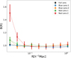 |
Fig. 5. Boost factors B(R) for the background source sample around the galaxies of FLS (black), Blue Lens-1 (blue) and -2 (orange), and Red Lens-1 (green) and -2 (red) in nine radial bins from approximately 0.03–1.2 h−1 Mpc. |
The B(R) of Blue Lens-1 tend to 1.0 at each radii in Fig. 5, which is similar to FLS, shows that the selection of lens–source pairs Δzp > 0.2 can clearly separate foreground lens and background sources out for the low-stellar-mass galaxies. The Blue Lens-2 and Red Lens-1 have slightly larger B(R) which tells us there is an increasing correlation between lenses and sources. Especially for high-stellar-mass galaxies such as those of the Red Lens-2 sample, the boost factor reflects the fact that there is an obvious correlation effect – as discussed above – for lens–sources pairs. This allows us to compute an ‘unbiased’ ΔΣ by multiplying the ΔΣ measured as in Sect. 4.2 by the boost factor B(R).
4.4. Covariance matrix
To estimate the statistical errors on ΔΣ(R), we apply a bootstrap method to the covariance matrix of the ΔΣ(R). The dimensionless covariance matrix can be simply calculated as
where Vi, j = ⟨(ΔΣ(Ri)−⟨ΔΣ(Ri)⟩)⋅(ΔΣ(Rj)−⟨ΔΣ(Rj)⟩)⟩, and this also works by changing the corresponding ‘i’ and ‘j’ for Vi, i and Vj, j. If the random signal ΔΣrand(R) is subtracted from ΔΣ(R), less covariance will be seen in the ESD measurements (Singh & Mandelbaum 2016).
We calculate the covariance matrix from the correlations between different ΔΣ(R), which are re-sampled by bootstrapping 104 times around the foreground galaxies from FLS objects. In our cases, the Hartlap correction (Hartlap et al. 2007) (Ns − Npoints − 2)/(Ns − 1) is negligible for the covariance matrix because it is very close to unity, where Ns = 104 is the number of simulations and Npoints = 9 is the number of data points. In Fig. 6, the off-diagonal terms show that there is no significant correlation in ΔΣ(R) between different radial bins, but on the contrary, there is strong self-correlation in ΔΣ(R), which is reflected in the diagonal of the covariance matrix. This means that ESDs from different radial bins are mutually independent in the galaxy–galaxy lensing signal. Furthermore, we can calculate the reduced χ2 to qualify the goodness of the fit between model and data using the equation

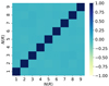 |
Fig. 6. Correlation matrix propagated from the estimated ΔΣ variance matrix of FLS in different radial bins according to the pipeline of bootstrapping. The label N(R) represents nine radial bins from approximately 0.03–1.2 h−1 Mpc. The colours from light yellow to deep blue indicate that the correlations of ΔΣ between radial bins are from weak to strong, respectively. |
where C−1 is the inverse covariance matrix, and degree of freedom d.o.f. = Npoints − Npara − 1, where Npara is the number of model parameters. Table 2 also shows the  for the model results corresponding to lens samples.
Posterior constraints derived from the best fitting to the ΔΣ measured around the galaxies from Blue Lens-1 and -2, Red Lens-1 and -2, and FLS by our halo model with responding reduced χ2 and p-value.
5. Weak lensing model
5.1. The model
The measurements of ΔΣ(R) can be derived from the galaxy–matter cross-correlation ξgm(r) so that the galaxy–galaxy lensing can provide an effective estimation of the dark matter halo profile and galaxy environment in the area around the lens. The ξgm(r) is the line-of-sight projection of galaxy–matter cross-correlation function, defined as (Luo et al. 2018)

which relates the surface mass density to a corresponding lens galaxy. The ESD would be calculated using Eq. (3):
![$$ \begin{aligned} \overline{\Sigma }(R) = 2\overline{\rho }\int ^{\infty }_{R}[1+\xi _{\rm gm}(r)]\frac{r \mathrm{d}r}{\sqrt{r^2-R^2}}, \end{aligned} $$](/articles/aa/full_html/2022/12/aa43758-22/aa43758-22-eq36.gif)
and
![$$ \begin{aligned} \overline{\Sigma }(\le R)=-\frac{4\overline{\rho }}{R^2}\int ^R_0{{ y} \mathrm{d}{ y}}\int ^{\infty }_{{ y}}[1+\xi _{\rm gm}(r)]\frac{r \mathrm{d}r}{\sqrt{r^2-{ y}^2}}, \end{aligned} $$](/articles/aa/full_html/2022/12/aa43758-22/aa43758-22-eq37.gif)
where  is the average background density of the Universe.
As Eq. (4) connects the observations with ΔΣ(R), it provides a method to estimate the distribution of the underlying dark matter in the foreground environments in the observed region by fitting observations to the halo model. In the following, we consider the total mass contributing to the ΔΣ(R), the calculation of which consists of two main terms: the one-halo term and two-halo term. The first term includes all the mass contained in stars, both from the central and satellite galaxies, and the dark matter main halo. The second term is the projected two-halo term that correlates the matter in other individual halos with the main host halo. In general, the contribution from one-halo term is dominated in the scales smaller than the virial radius of the host halo, and the two-halo term is forced to have an effect at the scales larger than the virial radius. According to this definition, the ESD can be written as

which does not contain the contribution from the average background density of the Universe, which does not give any contribution to the ESD, by definition.
5.1.1. One-halo term
The contributions from the one-halo term are all given by the mass elements inside of the host halo. Specifically, ΔΣ1h(R) is given by the three components: (1) the stellar mass density of the central galaxy, ΔΣ*(R), (2) the dark matter density of the central halo, ΔΣcen(R), and (3) the mass density of the satellite galaxies, ΔΣsat(R).
The stellar component, ΔΣ*(R), assumes the central galaxy as a point mass, and can be modelled as
where M* are the medians of the stellar mass of galaxies from different lens samples in our specific sample. As we measure the weak lensing signal starting from a distance that is generally a few tens of kiloparsec from the centre, the point-mass assumption is fairly reasonable.
For the other two components, such as the central dark halo and the overall satellite mass density, ΔΣcen(R) and ΔΣsat(R), we adopt a Navarro et al. (1997; hereafter NFW) density profile
where r is the distance from the halo centre, rs is the characteristic radius, and
where we further define the mean density as Δvir = 200 times the critical density of the Universe and a concentration parameter c = c200 = r200/rs, where r200 is the viral radius of the halo.
In Eqs. (14) and (15), we simply replace the  with the density distribution of the host halo ρ(r) as in Eq. (18). The projected ESD ΔΣcen (Yang et al. 2006) produced from the lensing signals γt around foreground central galaxies for an NFW profile is given by
![$$ \begin{aligned} \Delta \Sigma _{\rm cen}(R)=\frac{M_{\rm h}}{2\pi r^2_{\rm s}}I^{-1}[g(R/r_{\rm s})-f(R/r_{\rm s})], \end{aligned} $$](/articles/aa/full_html/2022/12/aa43758-22/aa43758-22-eq44.gif)
where the halo mass  ,
,
![$$ \begin{aligned} f(x)=\left\{ \begin{array}{l} \frac{1}{x^{2}-1}\left[1-\frac{\ln \left(\frac{1+\sqrt{1-x^{2}}}{x}\right)}{\sqrt{1-x^{2}}}\right] \text{,} x < 1, \\ \frac{1}{3} \text{,} x=1, \\ \frac{1}{x^{2}-1}\left[1-\frac{\text{ arctan}\left(\sqrt{x^{2}-1}\right)}{\sqrt{x^{2}-1}}\right] \text{,} x>1, \end{array}\right. \end{aligned} $$](/articles/aa/full_html/2022/12/aa43758-22/aa43758-22-eq46.gif)
and
![$$ \begin{aligned} g(x)=\left\{ \begin{array}{l} \frac{2}{x^{2}}\left[\ln \left(\frac{x}{2}\right)+\frac{\ln \left(\frac{1+\sqrt{1-x^{2}}}{x}\right)}{\sqrt{1-x^{2}}}\right] \text{,} x < 1, \\ 2+2 \ln \left(\frac{1}{2}\right) \text{,} x=1, \\ \frac{2}{x^{2}}\left[\ln \left(\frac{x}{2}\right)+\frac{\text{ arctan}\left(\sqrt{x^{2}-1}\right)}{\sqrt{x^{2}-1}}\right] \text{,} x>1, \end{array}\right. \end{aligned} $$](/articles/aa/full_html/2022/12/aa43758-22/aa43758-22-eq47.gif)
with x = R/rs.
The satellite component, ΔΣsat(R), is further composed of two contributions: first, the ESD contributed from the host halo of the satellite galaxy, ΔΣs, host(R|Rsat), and second, the dark matter subhalo, ΔΣs, sub(R). The total satellite ESD can therefore be written as

where Rsat is the projected off-centre distance between the satellite galaxy, which is located at the centre of its subhalo, and the centre of its host halo. The projected surface mass density of the host halo around a satellite galaxy at Rsat can be given by

where ΣNFW is the projected density profile of the host halo.
According to Eq. (3), we can calculate the ESD of the host halo of the satellite galaxy by

where the Σs, host(R ≤ Rsat) can be derived by the integral of the Σs, host(R|Rsat) from 0 to R. The subhalo contribution is derived from the density profiles of stripped dark matter subhalos, as described in Hayashi et al. (2003).
In our model, we apply a simple power-law HOD model for the satellite occupation function as studied in Mandelbaum et al. (2005b), Mandelbaum et al. (2009) assuming an NFW profile of the satellite distribution, so that
where P(Rsat|Mh) is simply the f(x) in Eq. (21). The ⟨Nsat⟩(Mh) is the occupation function of satellite galaxies given a halo mass Mh. The n(Mh) is the halo mass function based on Tinker et al. (2005).
Finally, the one-halo term is composed of the stellar mass contribution with the dark halo contributions, which are weighted by the satellite fraction, from the central and satellite galaxies:

The halo mass Mh is mostly provided by the total mass of the one-halo term that embraces the baryons and the NFW virial mass M200, which represents the mean density is 200 times the critical density within the radius r200.
5.1.2. Two-halo term
The two-halo term arises from the matter of the satellite galaxies in neighbouring halos that are correlated with the large-scale distribution of dark matter in the host halos (Yang et al. 2006). As the scale increases, the two-halo term is supposed to gradually dominate the ESD signals. In order to obtain the ESD from the contribution of the two-halo term, we apply pyCamb (Lewis 2013) to calculate the power spectrum at the median redshift of each sample. The matter–matter correlation function ξmm can then be converted by the power spectrum. Next, we use ξmm to calculate the halo–matter correlation function ξhm using the scale-dependent bias model (Tinker et al. 2005),
where
and bh(Mh) is the halo bias (Seljak & Warren 2004) as a function of the halo mass. The two-halo term ΔΣ2h can then be estimated using Eq. (3).
5.2. Fitting process
Given the halo model defined above, the measured ESD is used to constrain the halo properties of the corresponding lens sample. Specifically we want to constrain the three free parameters of the model, that is, the virial halo mass, Mh, the concentration, c, of the one-halo term, and the satellite fraction, fsat.
To best fit the observed EDS, we use the emcee (Foreman-Mackey et al. 2013) Python pipeline, which makes use of a standard MCMC procedure (Luo et al. 2022) to explore the likelihood function in the multidimensional parameter space. The maximum likelihood function is a Gaussian where the covariance matrix is estimated by bootstrap sampling. In our analysis, we have adopted a flat prior distribution with the host halo mass log(Mh/M⊙) in the range [9.5, 14.0], the concentration c in the range [0.1, 20.0], and the satellite fraction, fsat in the range [0.0, 1.0]. We set a rather broad range for the parameter space in order to reduce the prior effects by as much as possible.
6. Results
6.1. Testing for systematic errors
The assessment of systematic errors is a crucial part of the galaxy–galaxy lensing analysis, as these impact the reliability of the results. The first test is related to the B-mode signal. This represents the cross components of the galaxy–galaxy lensing signals, γ×, along a direction tilted by 45° with respect to the tangential component, γt. The γt itself produces an ESD cross component, ΔΣ×, tilted with respect to the tangential components, ΔΣ. By definition, the B-mode signal is zero for an unbiased shear signal. Therefore, any deviation from zero can indicate the presence of systematic error in the ESD, which is diluted by the presence of off-axis shear. Figure 7 shows the B-mode signals ΔΣ× for the VOICE FLS. This is generally consistent with zero for all scales, as expected for lensing; although the innermost ΔΣ× point slightly deviates from zero. The B-mode tests for the Red Lens and Blue Lens subsamples is discussed in detail in Appendix A. These also show almost no systematic errors, although the error bars become, in some cases, rather large. As the ΔΣ× are almost all consistent with zero, we conclude that the systematic errors, if any, are reasonably confined within the statistical errors.
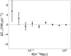 |
Fig. 7. Test for systematic errors in the B-mode signal for the galaxy–galaxy lensing measurements. The black points with error bars represent the ‘B-mode signals’ ΔΣ×, the cross component of lensing signals from the background sources, measured around the galaxies of the FLS. |
We generated 100 times as many random points in the random lens samples as the number of galaxies in our lens samples that correspond to the FLS and Blue Lens-1 and -2 and Red Lens-1 and -2, respectively. Figure 8 shows the ESD signals ΔΣrand of background sources, measured around the random points from the FLS. These are, again, fairly consistent with zero overall, with marginal evidence of a positive signal in the first bin. The results for the Red Lens and Blue Lens subsamples are discussed in detail in Appendix A. They show a similar pattern, with random signal generally consistent with zero.
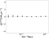 |
Fig. 8. Test for systematic errors in the random-point signal for galaxy–galaxy lensing measurements. The black points with error bars represent the ΔΣrand, the tangential component of lensing signals from the same source sample, measured around points of the random lens sample corresponding to the FLS. |
A final note of caution is needed about the innermost bin at ∼27 kpc h−1, corresponding to ∼9″ in angular scale. In both tests above, we have stressed a marginal systematic deviation of the ΔΣ× and ΔΣrand from zero. There are two possible explanations that can mitigate the impact of this source of systematic error. On the one hand, the lens sample dominated by faint galaxies with low stellar mass is different from that of Sifón et al. (2018), who find an additive bias as a bright lens influences the shapes of background sources at small scale. Therefore, the effect is negligible for the faint galaxies of our lens samples at this small scale. On the other hand, the ΔΣ× and ΔΣrand represent the systematic errors that should tend to zero, but it is reasonable that both deviate from zero if the counts of lens–source pairs decrease. Importantly, the area of the innermost bin is smaller than those of the outer bins, and therefore there are less counts of sources around the lens at the smaller scale, which leads to the greater deviation from zero for the innermost ESD measurements. However, the ΔΣ× and ΔΣrand for all radial bins are within 2σ, meaning that there are acceptable systematic errors, and that we can keep the innermost ESD measurements.
6.2. Halo property constraints
In this section, we present the halo model constraints of the VOICE lens samples using the MCMC procedure introduced in Sect. 5.2 to fit the ESD signals produced by the source sample.
The ΔΣ for the FLS are shown as blue points with error bars in Fig. 9. The error bars for ΔΣ are calculated from the standard errors based on the bootstrap via re-sampling 104 times. In the same figure, the blue solid curve is the best-fit line to the ESDs of the FLS, which is given by the total model as the sum of all contributions of the different mass components defined by the free parameters. More specifically, (1) the orange dash-dotted line represents the contribution from the stellar mass of foreground galaxies, which is defined by the median stellar mass derived from the stellar population analysis; (2) the green dashed line is the NFW model defined by the best-fit parameters c and Mh; (3) the red dashed line represents the satellite galaxies, defined by the other free parameter fsat; and (4) the black dotted line describes the contribution from the two-halo term. These contributions are described in detail in Sect. 5.1.
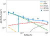 |
Fig. 9. ESD signals (ΔΣ) around FLS galaxies (blue points with bars), and the best fitting curve (blue solid line) comprised of the contribution from different components, namely the stellar term (orange dash-dotted line), the central term (green dashed line), the satellite term (red dashed line), and the two-halo term (black dotted line). |
From Fig. 9, it is clear that the satellite component and the two-halo term dominate the large scale, while the stellar mass and mostly the dark halo dominate on small scales. Overall, the total fit is reasonably good, with a reduced χ2 ≈ 1.995 (d.o.f. = 5, see Table 2).
The marginalised posterior distributions of the three parameters obtained for the FLS sample are shown in Fig. 10. The three contours correspond, from the innermost to the outermost one, to 16%, 50%, 84% confidence levels. For the FLS, the median host halo mass is 1011.42 M⊙, which, compared to the stellar mass M*, implies a Mh/M* = 102.93. It is evident from both Mh and M* that the sample is dominated by low-mass systems, as also discussed in Sect. 3.2.
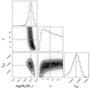 |
Fig. 10. Marginalised posterior distributions of three parameters obtained using the MCMC method for halo model to fit our ESD measurements around the galaxies of the FLS. The three contour levels, from the innermost to the outermost, correspond to the 16%, 50%, and 84% confidence levels, respectively. The blue points and lines are the medians. |
To explore the stellar-to-dark-matter relation, we proceed to best fit the other samples split by mass and colour, as defined in Sect. 3.2. Figure 11 shows the best-fit models with contributions from the different components for the ΔΣ from Red Lens and Blue Lens subsamples in the different mass bins adopted. We find that the corrected ΔΣ of Blue Lens-1 dropped at the large scale due to the subtraction. The value of the blue low-mass bin signal (ΔΣ = 0.18) is too small for the subtraction which means it is sensitive to ΔΣrand at the large scale for low-mass lenses. We therefore measure the reduced chi-square  with and without the last data point (d.o.f. = 5 and 4, respectively) presented in Table 2. Subtracting the outermost data point does not change the halo mass significantly, and we think the model fitting is generally consistent with the data points because the
  is 1.644 with a p-value of 0.160.
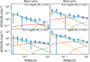 |
Fig. 11. Model fitting curves from MCMC procedure for the ΔΣ signals measured around Blue Lens-1 (top left panel), Blue Lens-2 (bottom left panel), Red Lens-1 (top right panel), and Red Lens-2 (bottom right panel). The best-fitting curve (blue solid line) is comprised of the contribution from different components that are stellar term (orange dash-dotted line), central term (green dashed line), satellite term (red dashed line), and two-halo term (black dotted line), respectively. |
Here we can appreciate the variance of ΔΣ amplitude as a function of sample mass. In particular, the central peak of the most massive (red) sample (bottom-right panel) is one order of magnitude larger than that of the least massive (blue) sample. Looking at the typical systematic errors from the cross and random samples (see Appendix. A), it is evident that these are negligible with respect to the signal of the massive samples (log M*/M⊙ > 9.5), while they might affect the low-mass sample (log M*/M⊙ < 9.5). Another evident feature is that the stellar component seems to be more centrally concentrated for the massive systems than for the less massive ones, while the satellite fraction decreases with stellar mass (see also Table 2).
Overall, the total model allows us to fit the ESD measurements of Blue Lens-1 and -2 and Red Lens-1 and -2 rather well, with better reduced χ2 than that of the FLS (see Table 2). The halo masses Mh of the four samples show a positive relation with stellar mass M*, which is physically reasonable. On the other hand, the concentration c does not show a clear (anti-)correlation with the virial mass, as predicted from simulations (e.g., Neto et al. 2007).
To conclude this section, we compare the stellar-to-halo mass relation (SHMR) found here with those of the literature. Figure 12 shows comparisons between the SHMR results from Red Lens and Blue Lens subsamples in similar redshift ranges and seven different curves, which are the results from three models and galaxy–galaxy lensing (GGL) analyses of three surveys: abundance matching (AM; Girelli et al. 2020; Rodríguez-Puebla et al. 2017), empirical modelling (EM; Behroozi et al. 2019), and the conditional luminosity function or halo occupation distribution (CLF/HOD; Yang et al. 2012); CFHTLenS (Hudson et al. 2015), KiDS+GAMA (Dvornik et al. 2020) and HSC (Wang et al. 2021). As we can see in Fig. 12, the SHMRs of Blue Lens-2 and Red Lens-1 and -2 show good agreements with the results from other studies, but Blue Lens-1 is situated below these curves, which means the stellar mass is lower than those predictions at a certain low halo mass.
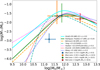 |
Fig. 12. Relation of the fraction of stellar and halo mass vs. halo mass. The circular points with cross error bars are the SHMR results of Blue Lens-1 (blue) and -2 (orange) and Red Lens-1 (green) and -2 (red), respectively. For comparison, here displayed are the SHMR results from different models: AM (the cyan and green solid lines), EM (the orange dashed line), and CLF/HOD(the sea-blue dashed line). Also displayed are galaxy–galaxy lensing results from the surveys of CFHTLenS (the magenta dotted line), KiDS+GAMA (the red dotted line), and HSC (the blue dotted line). |
7. Discussion and conclusions
We measure the galaxy–galaxy lensing signals around galaxies selected from the VOICE photometric catalogue by stacking the background galaxy shape behind them. The shape catalogue is based on the full VOICE photometric catalogue but with selection criteria designed for weak lensing analysis as described in F18. In this section, we discuss our major results and draw some conclusions.
The 4.9 deg2 multi-band VOICE deep imaging survey overlaps with the Chandra Deep Field-South (CDFS) region. The depth is down to 26.1 (5σ limiting magnitude) in the r band. We selected the full lens sample (FLS) between redshift 0.1 < zl(BPZ) < 0.35 and further split it into four subsamples based on stellar mass and colour. During the stacking process, we selected the background galaxies to be at a higher redshift than the lens sample, such as zs > zl + 0.2, in order to avoid contamination from the unlensed galaxies. A boost factor was applied to each measurement as a correction for the residual contamination induced by the effect of lens–source physical correlation.
We carried out a series of tests to assess the systematic errors in the measurements, including the B-mode test and random samples test. Both null tests are consistent with zero for all the samples except the ESDs of the innermost radial bins. We find it acceptable that these innermost ESDs are within 1 ∼ 2σ for FLS and the Blue Lens samples and within 1σ for the Red Lens samples. We also cross tested the reliability using the DES-Y1 public shape catalogue in the VOICE region, and find the results are consistent with each other, regardless of the different shape measurement methods (LensFit for VOICE and METACALIBRATION for DES). On the other hand, the DES measurements are noisier than VOICE measurements, which is due to the shallower survey depth of DES (see Appendix B).
Due to the fact that Σcrit depends on the photo-z of sources around each lens, the redshift uncertainties will influence the ESD measurement. In order to test this effect, we selected sources around each lens where the accumulated probability of the photo-z of each source satisfies the requirement (Medezinski et al. 2018) P(zs > zl + 0.2) > 0.98, and then we corrected Σcrit by applying the P(zs) to marginalise over photo-z errors according to Luo et al. (2022). However, this selection leads to larger statistical errors in the ESD measurements, because it significantly reduces the number of sources around each lens. We obtained consistent ESD measurements when using (see Appendix C) and not using (see Sect. 6.2) this method for our samples, but the bootstrap error bars of the former ESD measurements are larger than those of the latter. We decided not to apply the full p(z) in the ESD measurement for our samples. On the other hand, F18 presented the photo-z (BPZ) accuracy in detail, and we think that taking into account the photo-z uncertainties of sources is sufficient.
We then fit the ESDs with a three-parameter model, which includes halo mass, concentration of the halo, and satellite fraction. For the FLS, we estimate the halo mass to be  , the concentration parameter
  , and the satellite fraction
  . For the lens subsamples, we checked the stellar mass to halo mass relation (SHMR) and compared our results to various existing SHMR models (Fig. 12).
We find that the blue low-mass lens sample Blue Lens-1 (median M* = 108.31 M⊙) shows significantly larger halo mass than theoretical predictions, while the other subsamples are consistent with theory. This result is in agreement with the findings of Hudson et al. (2015), who showed that the mass to light ratio of the faint blue dwarfs deviates towards higher values than what is suggested by the abundance matching prediction. Boylan-Kolchin et al. (2012) also showed similar results for low-mass galaxies from dynamical analysis. The rotation curve analysis by Ferrero et al. (2012) again shows similar results for dwarf galaxies. Interestingly, the opposite appears to be true for massive star forming galaxies where the halo mass is much lower than the theoretical predictions by Zhang et al. (2021), indicating a very high gas-to-stellar-mass conversion rate (up to 67%) at stellar masses of around 1010.75 M⊙.
Another interesting finding of our work is that the blue dwarf galaxies, that is, members of the Blue Lens-1 sample, make up ∼75% of the full sample, implying that the VOICE-CDFS region is dominated by low-mass blue dwarf galaxies in the redshift range of our FLS. This result agrees with the work from Phleps et al. (2007), who estimated the overdensities of three COMBO-17 fields, and found that the CDFS region density is two times lower than the other two regions, which agrees with local 2dF observations. We therefore suggest that any cosmological constraints using the data in this region may suffer from severe cosmic variance in this particular redshift range.
In this first paper of our galaxy–galaxy lensing study from VOICE deep imaging data, we test the robustness of our measurement and obtain the SHMR for lens samples of red and blue galaxies binned according to stellar mass. Deep imaging data would enable a galaxy–galaxy lensing analysis for objects of even higher redshift. In the future, combining X-ray data from CDFS, we will further explore the halo properties of X-ray-selected AGNs using the VOICE shape catalogue (Li et al., in prep.).
Acknowledgments
The corresponding authors are Liping Fu, Wentao Luo, and Nicola R. Napolitano. RL acknowledges the supports from Sun Yat-sen University and Shanghai Normal University for the numerical computations are carried out through Kunlun cluster of SYSU and the computer cluster of SHNU. LF acknowledges the supports from NSFC grants 11933002, and the Dawn Program 19SG41 and the Innovation Program 2019-01-07-00-02-E00032 of SMEC. WL is supported in part by the National Key R&D Program of China (2021YFC2203100), the NSFC (No.11833005, 12192224). We acknowledge the science resarch grants from the China Manned Space Project with No. CMS-CSST-2021-A01. N.R.N acknowledge financial support from the One hundred top talent program of Sun Yat-sen University grant N. 71000-18841229. MV acknowledges financial support from the Inter-University Institute for Data Intensive Astronomy (IDIA), a partnership of the University of Cape Town, the University of Pretoria, the University of the Western Cape and the South African Radio Astronomy Observatory, and from the South African Department of Science and Innovation’s National Research Foundation under the ISARP RADIOSKY2020 Joint Research Scheme (DSI-NRF Grant Number 113121) and the CSUR HIPPO Project (DSI-NRF Grant Number 121291).
References
- Abbott, T. M. C., Abdalla, F. B., Alarcon, A., et al. 2018, Phys. Rev. D, 98, 043526 [NASA ADS] [CrossRef] [Google Scholar]
- Aihara, H., Armstrong, R., Bickerton, S., et al. 2018, PASJ, 70, S8 [NASA ADS] [Google Scholar]
- Arnouts, S., Cristiani, S., Moscardini, L., et al. 1999, MNRAS, 310, 540 [Google Scholar]
- Baldry, I. K., Glazebrook, K., Brinkmann, J., et al. 2004, ApJ, 600, 681 [Google Scholar]
- Bartelmann, M., & Schneider, P. 2001, Phys. Rep., 340, 291 [Google Scholar]
- Behroozi, P. S., Conroy, C., & Wechsler, R. H. 2010, ApJ, 717, 379 [Google Scholar]
- Behroozi, P., Wechsler, R. H., Hearin, A. P., & Conroy, C. 2019, MNRAS, 488, 3143 [NASA ADS] [CrossRef] [Google Scholar]
- Bell, E. F., McIntosh, D. H., Katz, N., & Weinberg, M. D. 2003, ApJS, 149, 289 [Google Scholar]
- Benítez, N. 2011, Astrophysics Source Code Library [record ascl:1108.011] [Google Scholar]
- Berlind, A. A., & Weinberg, D. H. 2002, ApJ, 575, 587 [Google Scholar]
- Blumenthal, G. R., Faber, S. M., Flores, R., & Primack, J. R. 1986, ApJ, 301, 27 [Google Scholar]
- Boylan-Kolchin, M., Bullock, J. S., & Kaplinghat, M. 2012, MNRAS, 422, 1203 [NASA ADS] [CrossRef] [Google Scholar]
- Brainerd, T. G., Blandford, R. D., & Smail, I. 1996, ApJ, 466, 623 [NASA ADS] [CrossRef] [Google Scholar]
- Bruzual, G., & Charlot, S. 2003, MNRAS, 344, 1000 [NASA ADS] [CrossRef] [Google Scholar]
- Cacciato, M., van den Bosch, F. C., More, S., et al. 2009, MNRAS, 394, 929 [NASA ADS] [CrossRef] [Google Scholar]
- Cacciato, M., van den Bosch, F. C., More, S., Mo, H., & Yang, X. 2013, MNRAS, 430, 767 [Google Scholar]
- Calzetti, D., Kinney, A. L., & Storchi-Bergmann, T. 1994, ApJ, 429, 582 [Google Scholar]
- Capaccioli, M., & Schipani, P. 2011, The Messenger, 146, 2 [NASA ADS] [Google Scholar]
- Chabrier, G. 2003, PASP, 115, 763 [Google Scholar]
- Clampitt, J., Sánchez, C., Kwan, J., et al. 2017, MNRAS, 465, 4204 [NASA ADS] [CrossRef] [Google Scholar]
- Conroy, C., & Wechsler, R. H. 2009, ApJ, 696, 620 [NASA ADS] [CrossRef] [Google Scholar]
- Conroy, C., Wechsler, R. H., & Kravtsov, A. V. 2006, ApJ, 647, 201 [Google Scholar]
- Cooray, A., & Sheth, R. 2002, Phys. Rep., 372, 1 [Google Scholar]
- Dark Energy Survey Collaboration (Abbott, T., et al.) 2016, MNRAS, 460, 1270 [Google Scholar]
- Davé, R., Finlator, K., & Oppenheimer, B. D. 2012, MNRAS, 421, 98 [Google Scholar]
- Drlica-Wagner, A., Sevilla-Noarbe, I., Rykoff, E. S., et al. 2018, ApJS, 235, 33 [Google Scholar]
- Dvornik, A., Hoekstra, H., Kuijken, K., et al. 2020, A&A, 642, A83 [NASA ADS] [CrossRef] [EDP Sciences] [Google Scholar]
- Faucher-Giguère, C.-A., Kereš, D., & Ma, C.-P. 2011, MNRAS, 417, 2982 [CrossRef] [Google Scholar]
- Ferrero, I., Abadi, M. G., Navarro, J. F., Sales, L. V., & Gurovich, S. 2012, MNRAS, 425, 2817 [Google Scholar]
- Flaugher, B., Diehl, H. T., Honscheid, K., et al. 2015, AJ, 150, 150 [Google Scholar]
- Foreman-Mackey, D., Hogg, D. W., Lang, D., & Goodman, J. 2013, PASP, 125, 306 [Google Scholar]
- Franzen, T. M. O., Banfield, J. K., Hales, C. A., et al. 2015, MNRAS, 453, 4020 [Google Scholar]
- Fu, L., Kilbinger, M., Erben, T., et al. 2014, MNRAS, 441, 2725 [Google Scholar]
- Fu, L., Liu, D., Radovich, M., et al. 2018, MNRAS, 479, 3858 [CrossRef] [Google Scholar]
- Fukugita, M., Hogan, C. J., & Peebles, P. J. E. 1998, ApJ, 503, 518 [NASA ADS] [CrossRef] [Google Scholar]
- Geiger, B., & Schneider, P. 1999, MNRAS, 302, 118 [NASA ADS] [CrossRef] [Google Scholar]
- Girelli, G., Pozzetti, L., Bolzonella, M., et al. 2020, A&A, 634, A135 [NASA ADS] [CrossRef] [EDP Sciences] [Google Scholar]
- Gong, Y., Liu, X., Cao, Y., et al. 2019, ApJ, 883, 203 [NASA ADS] [CrossRef] [Google Scholar]
- Guzik, J., & Seljak, U. 2002, MNRAS, 335, 311 [CrossRef] [Google Scholar]
- Hartlap, J., Simon, P., & Schneider, P. 2007, A&A, 464, 399 [NASA ADS] [CrossRef] [EDP Sciences] [Google Scholar]
- Hayashi, E., Navarro, J. F., Taylor, J. E., Stadel, J., & Quinn, T. 2003, ApJ, 584, 541 [Google Scholar]
- Heymans, C., Van Waerbeke, L., Miller, L., et al. 2012, MNRAS, 427, 146 [Google Scholar]
- Hoekstra, H., & Jain, B. 2008, Ann. Rev. Nucl. Part. Sci., 58, 99 [NASA ADS] [CrossRef] [Google Scholar]
- Hudson, M. J., Gillis, B. R., Coupon, J., et al. 2015, MNRAS, 447, 298 [Google Scholar]
- Huff, E., & Mandelbaum, R. 2017, ApJ, submitted [arXiv:1702.02600] [Google Scholar]
- Ilbert, O., Arnouts, S., McCracken, H. J., et al. 2006, A&A, 457, 841 [NASA ADS] [CrossRef] [EDP Sciences] [Google Scholar]
- Jarvis, M., Bernstein, G. M., Fischer, P., et al. 2003, AJ, 125, 1014 [NASA ADS] [CrossRef] [Google Scholar]
- Jarvis, M. J., Bonfield, D. G., Bruce, V. A., et al. 2013, MNRAS, 428, 1281 [Google Scholar]
- Jing, Y. P., Mo, H. J., & Börner, G. 1998, ApJ, 494, 1 [NASA ADS] [CrossRef] [Google Scholar]
- Kilbinger, M., Fu, L., Heymans, C., et al. 2013, MNRAS, 430, 2200 [Google Scholar]
- Kochanek, C. S. 1995, ApJ, 445, 559 [NASA ADS] [CrossRef] [Google Scholar]
- Kravtsov, A. V., Berlind, A. A., Wechsler, R. H., et al. 2004, ApJ, 609, 35 [Google Scholar]
- Kuijken, K. 2011, The Messenger, 146, 8 [NASA ADS] [Google Scholar]
- Kuijken, K., Heymans, C., Hildebrandt, H., et al. 2015, MNRAS, 454, 3500 [Google Scholar]
- Kuijken, K., Heymans, C., Dvornik, A., et al. 2019, A&A, 625, A2 [NASA ADS] [CrossRef] [EDP Sciences] [Google Scholar]
- Kwan, J., Sánchez, C., Clampitt, J., et al. 2017, MNRAS, 464, 4045 [NASA ADS] [CrossRef] [Google Scholar]
- Lee, S., Troxel, M. A., Choi, A., et al. 2022, MNRAS, 509, 2033 [Google Scholar]
- Lewis, A. 2013, Phys. Rev. D, 87 [CrossRef] [Google Scholar]
- Liu, D., Fu, L., Liu, X., et al. 2018, MNRAS, 478, 2388 [Google Scholar]
- Lonsdale, C. J., Smith, H. E., Rowan-Robinson, M., et al. 2003, PASP, 115, 897 [Google Scholar]
- LSST Science Collaboration (Abell, P. A., et al.) 2009, ArXiv e-prints [arXiv:0912.0201] [Google Scholar]
- Luo, W., Yang, X., Lu, T., et al. 2018, ApJ, 862, 4 [Google Scholar]
- Luo, W., Silverman, J. D., More, S., et al. 2022, ApJ, accepted [arXiv:2204.03817] [Google Scholar]
- Mandelbaum, R., Hirata, C. M., Seljak, U., et al. 2005a, MNRAS, 361, 1287 [Google Scholar]
- Mandelbaum, R., Tasitsiomi, A., Seljak, U., Kravtsov, A. V., & Wechsler, R. H. 2005b, MNRAS, 362, 1451 [NASA ADS] [CrossRef] [Google Scholar]
- Mandelbaum, R., Seljak, U., Kauffmann, G., Hirata, C. M., & Brinkmann, J. 2006, MNRAS, 368, 715 [NASA ADS] [CrossRef] [Google Scholar]
- Mandelbaum, R., Li, C., Kauffmann, G., & White, S. D. M. 2009, MNRAS, 393, 377 [Google Scholar]
- Mandelbaum, R., Slosar, A., Baldauf, T., et al. 2013, MNRAS, 432, 1544 [NASA ADS] [CrossRef] [Google Scholar]
- Martin, D. C., Fanson, J., Schiminovich, D., et al. 2005, ApJ, 619, L1 [Google Scholar]
- Mauduit, J. C., Lacy, M., Farrah, D., et al. 2012, PASP, 124, 714 [Google Scholar]
- McKay, T. A., Sheldon, E. S., Johnston, D., et al. 2002, ApJ, 571, L85 [NASA ADS] [CrossRef] [Google Scholar]
- Medezinski, E., Oguri, M., Nishizawa, A. J., et al. 2018, PASJ, 70, 30 [NASA ADS] [Google Scholar]
- Miller, L., Heymans, C., Kitching, T. D., et al. 2013, MNRAS, 429, 2858 [Google Scholar]
- Morganson, E., Gruendl, R. A., Menanteau, F., et al. 2018, PASP, 130, 074501 [NASA ADS] [CrossRef] [Google Scholar]
- Moster, B. P., Somerville, R. S., Maulbetsch, C., et al. 2010, ApJ, 710, 903 [Google Scholar]
- Moster, B. P., Naab, T., & White, S. D. M. 2013, MNRAS, 428, 3121 [Google Scholar]
- Munshi, D., Valageas, P., van Waerbeke, L., & Heavens, A. 2008, Phys. Rep., 462, 67 [NASA ADS] [CrossRef] [Google Scholar]
- Natarajan, P., & Kneib, J.-P. 1997, MNRAS, 287, 833 [Google Scholar]
- Navarro, J. F., Frenk, C. S., & White, S. D. M. 1997, ApJ, 490, 493 [Google Scholar]
- Neto, A. F., Gao, L., Bett, P., et al. 2007, MNRAS, 381, 1450 [NASA ADS] [CrossRef] [Google Scholar]
- Oliver, S. J., Bock, J., Altieri, B., et al. 2012, MNRAS, 424, 1614 [NASA ADS] [CrossRef] [Google Scholar]
- Peacock, J. A., & Smith, R. E. 2000, MNRAS, 318, 1144 [Google Scholar]
- Phleps, S., Wolf, C., Peacock, J. A., Meisenheimer, K., & van Kampen, E. 2007, A&A, 468, 113 [NASA ADS] [CrossRef] [EDP Sciences] [Google Scholar]
- Prada, F., Vitvitska, M., Klypin, A., et al. 2003, ApJ, 598, 260 [NASA ADS] [CrossRef] [Google Scholar]
- Refregier, A., Amara, A., Kitching, T. D., et al. 2010, ArXiv e-prints [arXiv:1001.0061] [Google Scholar]
- Rodríguez-Puebla, A., Primack, J. R., Avila-Reese, V., & Faber, S. M. 2017, MNRAS, 470, 651 [Google Scholar]
- Schaye, J., Crain, R. A., Bower, R. G., et al. 2015, MNRAS, 446, 521 [Google Scholar]
- Seljak, U. 2000, MNRAS, 318, 203 [Google Scholar]
- Seljak, U., & Warren, M. S. 2004, MNRAS, 355, 129 [CrossRef] [Google Scholar]
- Sheldon, E. S., & Huff, E. M. 2017, ApJ, 841, 24 [NASA ADS] [CrossRef] [Google Scholar]
- Sheldon, E. S., Johnston, D. E., Frieman, J. A., et al. 2004, AJ, 127, 2544 [Google Scholar]
- Sifón, C., Herbonnet, R., Hoekstra, H., van der Burg, R. F. J., & Viola, M. 2018, MNRAS, 478, 1244 [Google Scholar]
- Singh, S., & Mandelbaum, R. 2016, MNRAS, 457, 2301 [NASA ADS] [CrossRef] [Google Scholar]
- Somerville, R. S., & Davé, R. 2015, ARA&A, 53, 51 [Google Scholar]
- Spergel, D., Gehrels, N., Baltay, C., et al. 2015, ArXiv e-prints [arXiv:1503.03757] [Google Scholar]
- The Dark Energy Survey Collaboration 2005, ArXiv e-prints [arXiv:astro-ph/0510346] [Google Scholar]
- Tinker, J. L., Weinberg, D. H., Zheng, Z., & Zehavi, I. 2005, ApJ, 631, 41 [Google Scholar]
- Treu, T. 2010, ARA&A, 48, 87 [NASA ADS] [CrossRef] [Google Scholar]
- Vaccari, M., Covone, G., Radovich, M., et al. 2016, in The 4th Annual Conference on High Energy Astrophysics in Southern Africa (HEASA 2016), 26 [Google Scholar]
- Vaccari, M., Marchetti, L., Franceschini, A., et al. 2010, A&A, 518, L20 [NASA ADS] [CrossRef] [EDP Sciences] [Google Scholar]
- Vale, A., & Ostriker, J. P. 2004, MNRAS, 353, 189 [Google Scholar]
- Vale, A., & Ostriker, J. P. 2006, MNRAS, 371, 1173 [NASA ADS] [CrossRef] [Google Scholar]
- van Uitert, E., Joachimi, B., Joudaki, S., et al. 2018, MNRAS, 476, 4662 [NASA ADS] [CrossRef] [Google Scholar]
- Viola, M., Cacciato, M., Brouwer, M., et al. 2015, MNRAS, 452, 3529 [NASA ADS] [CrossRef] [Google Scholar]
- Vogelsberger, M., Genel, S., Springel, V., et al. 2014, MNRAS, 444, 1518 [Google Scholar]
- Wang, W., Li, X., Shi, J., et al. 2021, ApJ, 919, 25 [NASA ADS] [CrossRef] [Google Scholar]
- Wechsler, R. H., & Tinker, J. L. 2018, ARA&A, 56, 435 [NASA ADS] [CrossRef] [Google Scholar]
- White, S. D. M., & Rees, M. J. 1978, MNRAS, 183, 341 [Google Scholar]
- Yang, X. H., Mo, H. J., Kauffmann, G., & Chu, Y. Q. 2003, MNRAS, 339, 387 [CrossRef] [Google Scholar]
- Yang, X., Mo, H. J., van den Bosch, F. C., et al. 2006, MNRAS, 373, 1159 [Google Scholar]
- Yang, X., Mo, H. J., van den Bosch, F. C., Zhang, Y., & Han, J. 2012, ApJ, 752, 41 [NASA ADS] [CrossRef] [Google Scholar]
- York, D. G., Adelman, J., Anderson, J. E., Jr, et al. 2000, AJ, 120, 1579 [Google Scholar]
- Zaritsky, D., & White, S. D. M. 1994, ApJ, 435, 599 [NASA ADS] [CrossRef] [Google Scholar]
- Zehavi, I., Zheng, Z., Weinberg, D. H., et al. 2005, ApJ, 630, 1 [Google Scholar]
- Zhan, H. 2011, Sci. Sin. Phys. Mech. Astron., 41, 1441 [NASA ADS] [CrossRef] [Google Scholar]
- Zhan, H. 2018, in 42nd COSPAR Scientific Assembly, 42, E1.16-4-18 [Google Scholar]
- Zhang, Z., Wang, H., Luo, W., et al. 2021, A&A, 663, A85 [Google Scholar]
- Zheng, Z., Berlind, A. A., Weinberg, D. H., et al. 2005, ApJ, 633, 791 [NASA ADS] [CrossRef] [Google Scholar]
- Zu, Y., & Mandelbaum, R. 2016, MNRAS, 457, 4360 [NASA ADS] [CrossRef] [Google Scholar]
- Zuntz, J., Sheldon, E., Samuroff, S., et al. 2018, MNRAS, 481, 1149 [Google Scholar]
Appendix A: Systematic errors for subsamples
In the Sect. 3.2, we separated the FLS into four lens samples of Blue Lens−1 and -2 and Red Lens−1 and -2. Here we show some results of tests for systematic errors and ESD measurements around the foreground galaxies of Red Lens and Blue Lens subsamples based on the same background source sample of VOICE. We measured the systematic errors of cross components ΔΣ× for the four lens samples in Fig. A.1 and of ΔΣrand around the lens galaxies of the four random point samples in Fig. A.2, respectively. There are obvious, large statistical errors at small scales due to the small galaxy numbers. However, the results of cross components and the ESDs of random points can be considered acceptable systematic errors because they are consistent with zero when the scale increases.
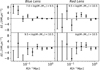 |
Fig. A.1. Test for systematic errors in the B-mode signals. Top and bottom left panels show the cross-components of ΔΣ measured around the galaxies of Blue Lens-1 and -2. The ΔΣ× in the top and bottom right panels are measured around the galaxies of Red Lens-1 and -2. |
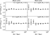 |
Fig. A.2. Test for systematic errors in the random-point signals. Top and bottom left panels and top and bottom right panels show the ΔΣrand measured around random points counted 100 times of the galaxies in Blue Lens-1 and -2 and Red-1 and -2 samples, respectively. |
Appendix B: Measurements with DES-Y1 data
In order to verify the reliability of halo properties in the VOICE− CDFS region, we compare VOICE with the results based on the Dark Energy Survey (DES) Year-one annual Data2 (Y1A1 or Y1) which was chosen for comparison because of its very similar but not complete coverage (∼93%) with VOICE−CDFS in DES−Y1. The DES (Dark Energy Survey Collaboration 2016) is a large imaging survey that uses 3 deg2 Dark Energy Camera (DECam; Flaugher et al. 2015), a Megapixel camera installed at prime focus on the Blanco 4-m telescope at the Cerro Tololo Inter-American Observatory in northern Chile (Morganson et al. 2018). The DES survey plans to cover a ∼1800 deg2 wide-area with exposures in grizY bands (Drlica-Wagner et al. 2018), which is fewer than the nine bands in the VOICE survey project and provides less exposure time than the VOICE survey for the corresponding band. The DES−Y1 shear measurements are based on the i band images with a median seeing of ∼0.99 arcsec (Morganson et al. 2018) which is slightly poorer than the selected exposure seeing which is ≤0.9 arcsec in VOICE r band images. Although the depth of DES is shallower than the VOICE survey, the comparison of galaxy–galaxy lensing results between VOICE and DES is a meaningful cross check for the results of halo properties in VOICE−CDFS region.
B.1. DES-Y1 Shear catalogue
Here we use the shear catalogue from DES projects to measure the ESD signal around FLS galaxies in order to verifys the reliability of ESD measurements from the VOICE shear catalogue. Zuntz et al. (2018) introduces two independent catalogues of galaxy shape measurements from DES−Y1 Data and one of them is called the METACALIBRATION (Huff & Mandelbaum 2017; Sheldon & Huff 2017) shear catalogue3 which covers 1500 deg2 of the Southern sky and contains 34.8 million objects. Based on the METACALIBRATION shear catalogue, we make a sample from a cut of the area that covers almost the same ranges of RA and DEC as the region of VOICE−CDFS, although the coverage of DES does not completely overlap. We then obtained the shear catalogue from DES−Y1 Data in the VOICE region (hereafter DES−V) which contains 244016 galaxies in 0.3 < zs(BPZ) < 1.5, which is the same redshift range as the background sources sample of VOICE. The 10σ limiting magnitude in i band for DES is ∼22.5, and the 5σ limiting magnitude in r band for VOICE is ∼26.1. The significant reason why there are fewer galaxies in the DES-V shear catalogue is that the VOICE survey can observe fainter objects than DES, inclusing objects that are at greater distances. In accordance with Lee et al. 2022, we estimate the average shear measurements as
where γt, j and  are the tangential shear measurements and the weight of the sources from the METACALIBRATION shear catalogue, and
  is the mean response averaged over the sources, which is defined as the sum of the average measured shear response Rγ and the shear selection bias correction matrix RS for METACALIBRATION:
The ESD measurements can then be derived using Eqs. (4)-(6). Furthermore, we make another shear catalogue by position matching for the galaxies from DES and VOICE shear catalogues that contains 148285 galaxies in 0.3 < zs(BPZ) < 1.5 and is referred to here as the matched background sources (MBS).
B.2. Comparison of measurements
In order to compare the differences in galaxy–galaxy lensing measurements between the background galaxies of VOICE and DES for the same lens sample, we decide to use FLS. Here we make two comparisons of VOICE versus DES in order to check the reliability of the ESD (ΔΣ) measurements from VOICE and the differences between two pipelines of shape measurements in Fig. B.1.
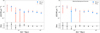 |
Fig. B.1. Comparison of ESD measurements for VOICE and DES. Left panel plots the ESDs around FLS with the background sources of VOICE and DES-V, and the right panel plots the ESDs around FLS with matched background sources for two surveys. The blue points and orange empty diamonds with error bars indicate the results based on the shape measurements in VOICE and DES surveys, respectively. The black points with error bars (the dex) represent the differences between the measurements from the VOICE relative to the DES. |
As a sanity check for the ESD measurements in the VOICE study, we measured the ΔΣ around FLS galaxies with the background sources from the DES−V shear catalogue under the selection of lens–source pair: Δzp > 0.2. We then compared the results of ΔΣ in the DES survey with those of the VOICE survey (see the left panel of Fig. B.1). Here we can see that the dex of the difference in ESD measurements from the two surveys in almost the same area is consistent with zero.
We also need to consider whether there are significant differences between the ESD measurements from the two kinds of shape measurement pipelines: Lensfit in VOICE and METACALIBRATION in DES. We therefore measured the ESDs around FLS galaxies and the MBS galaxies by different pipelines of the two surveys in the right panel of Fig. B.1. We find that the difference is almost consistent with zero. The difference in ΔΣ between the two surveys is within 2σ, and we find this very small discrepancy to be acceptable.
These comparisons of the results from DES survey with those of the VOICE survey suggest that the ESD measurements from VOICE are reliable for further VOICE galaxy–galaxy studies. The left panel of Fig. B.1 shows that the ΔΣ of VOICE and DES show good agreement, although the ESDs from the DES are noisier than those from VOICE. We believe this to be due to the fact that the galaxies in the DES survey are considered as stars or other contamination in the VOICE survey because of the different observational conditions of the two survey projects; the VOICE survey was carried out under better seeing conditions, and benefited from more exposure time, covers more observational bands, and so on.
We then matched the galaxies of shear catalogues of VOICE with DES within 1 arcsec separation. We further measured the ESDs around FLS with MBS from matched shear catalogues of VOICE and DES, respectively. The comparison of both is displayed in the right panel of Fig. B.1. The ΔΣ signals from DES are somewhat higher, and the dex of VOICE relative to DES (ΔΣVOICE − ΔΣDES) shows that there are very small shifts down from the measurements of VOICE to DES. We consider the main reason for the offset between the ESDs of the two surveys is that the shear catalogues of VOICE and DES are derived from different pipelines, namely Lensfit and METACALIBRATION, respectively. The offset is very weak which can be ignored, and it tells us that the shear measurement from Lensfit shows good agreement with that from METACALIBRATION. On the whole, the ESD measurements from VOICE and DES are consistent, and our results of VOICE deep survey study are reliable.
Appendix C: The effect of redshift uncertainty
The redshift uncertainty influences the ΔΣ measurements for each lens–source pair because the surface critical density Σcrit depends on the redshift uncertainty of sources around each lens. To check this effect, we measured ΔΣ of the FLS galaxies with the background sources selected so that the accumulated probability of photometric redshift (BPZ) P(zs > zl + 0.2) of each source is larger than 0.98 (Luo et al. 2022):
The critical surface density can then be calculated as
We find that assuming such a selection, there is a negligible difference between the ESD measurements ΔΣ(zs > zl + 0.2) in Fig. 9 and ΔΣ(P(zs > zl + 0.2) > 0.98) in Fig. C.1. However, error bars are larger, which is because there are fewer sources around each lens: this results in poorer model constraints (Fig. C.2) than those discussed in the main paper (Fig. 10). We therefore decided not to use the full p(z), considering that the difference is much smaller than the statistical error in our analysis.
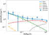 |
Fig. C.1. ESD signals ΔΣ(P(z > zl + 0.2) > 0.98) around FLS galaxies (blue points), and the best-fitting curve (blue solid line) is comprised of the contribution from different components, namely the stellar term (orange line), central term (green line), satellite term (red line), and the two-halo term (black line). |
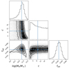 |
Fig. C.2. Marginalised posterior distributions of three parameters obtained using an MCMC method for the halo model to fit ΔΣ(P(z > zl + 0.2) > 0.98) around the galaxies of the FLS. The three contour levels, from outermost to innermost, correspond to 16%, 50%, 84% confidence levels, respectively. The blue points and lines are the medians. |
All Tables
Statistics of Red Lens-1 and -2, Blue Lens-1 and -2, and FLS with the mass bin range, numbers, median photo-z, and median logarithmic stellar mass.
Posterior constraints derived from the best fitting to the ΔΣ measured around the galaxies from Blue Lens-1 and -2, Red Lens-1 and -2, and FLS by our halo model with responding reduced χ2 and p-value.
All Figures
|
Fig. 1. Comparison of photo-z (Zphot) vs. spec-z (Zspec) for the matched galaxies (black points) sample (Fu et al. 2018). The contours present the galaxy number density. The red line is the one-to-one relation. |
| In the text | |
|
Fig. 2. Normalised distribution of photo-z (BPZ) for the galaxies of the Full Lens Sample (orange histogram) and Source Sample (green histogram). The distributions of the Red Lens and Blue Lens samples (red and blue dashed histogram, respectively) are normalised to the FLS. The redshift range of the FLS is 0.1 < zl < 0.35 and that of the Sources Sample is 0.3 < zs < 1.5. |
| In the text | |
|
Fig. 3. Distribution of colour [g − i] (rest-frame) vs. r-band absolute magnitude for the FLS. The colour coding of the points (from red to blue) represents increasing galaxy number density. The black dashed line is the criterion of [g − i]rest = 0.9 to separate red and blue galaxies. There are two sequences of galaxies in [g − i]rest > 0.9 and [g − i]rest < 0.9 that are considered as the galaxies of Red Lens and Blue Lens, respectively. |
| In the text | |
|
Fig. 4. Distribution of logarithmic stellar mass from Blue Lens (blue histogram) and Red Lens (red histogram). The Blue Lens-1 and 2 are from the logarithmic stellar mass bins of [7.0, 9.5] and [9.5, 10.5] in Blue Lens. The Red Lens-1 and 2 are from the logarithmic stellar mass bins of [9.5, 10.5] and > 10.5 in Red Lens. |
| In the text | |
|
Fig. 5. Boost factors B(R) for the background source sample around the galaxies of FLS (black), Blue Lens-1 (blue) and -2 (orange), and Red Lens-1 (green) and -2 (red) in nine radial bins from approximately 0.03–1.2 h−1 Mpc. |
| In the text | |
|
Fig. 6. Correlation matrix propagated from the estimated ΔΣ variance matrix of FLS in different radial bins according to the pipeline of bootstrapping. The label N(R) represents nine radial bins from approximately 0.03–1.2 h−1 Mpc. The colours from light yellow to deep blue indicate that the correlations of ΔΣ between radial bins are from weak to strong, respectively. |
| In the text | |
|
Fig. 7. Test for systematic errors in the B-mode signal for the galaxy–galaxy lensing measurements. The black points with error bars represent the ‘B-mode signals’ ΔΣ×, the cross component of lensing signals from the background sources, measured around the galaxies of the FLS. |
| In the text | |
|
Fig. 8. Test for systematic errors in the random-point signal for galaxy–galaxy lensing measurements. The black points with error bars represent the ΔΣrand, the tangential component of lensing signals from the same source sample, measured around points of the random lens sample corresponding to the FLS. |
| In the text | |
|
Fig. 9. ESD signals (ΔΣ) around FLS galaxies (blue points with bars), and the best fitting curve (blue solid line) comprised of the contribution from different components, namely the stellar term (orange dash-dotted line), the central term (green dashed line), the satellite term (red dashed line), and the two-halo term (black dotted line). |
| In the text | |
|
Fig. 10. Marginalised posterior distributions of three parameters obtained using the MCMC method for halo model to fit our ESD measurements around the galaxies of the FLS. The three contour levels, from the innermost to the outermost, correspond to the 16%, 50%, and 84% confidence levels, respectively. The blue points and lines are the medians. |
| In the text | |
|
Fig. 11. Model fitting curves from MCMC procedure for the ΔΣ signals measured around Blue Lens-1 (top left panel), Blue Lens-2 (bottom left panel), Red Lens-1 (top right panel), and Red Lens-2 (bottom right panel). The best-fitting curve (blue solid line) is comprised of the contribution from different components that are stellar term (orange dash-dotted line), central term (green dashed line), satellite term (red dashed line), and two-halo term (black dotted line), respectively. |
| In the text | |
|
Fig. 12. Relation of the fraction of stellar and halo mass vs. halo mass. The circular points with cross error bars are the SHMR results of Blue Lens-1 (blue) and -2 (orange) and Red Lens-1 (green) and -2 (red), respectively. For comparison, here displayed are the SHMR results from different models: AM (the cyan and green solid lines), EM (the orange dashed line), and CLF/HOD(the sea-blue dashed line). Also displayed are galaxy–galaxy lensing results from the surveys of CFHTLenS (the magenta dotted line), KiDS+GAMA (the red dotted line), and HSC (the blue dotted line). |
| In the text | |
|
Fig. A.1. Test for systematic errors in the B-mode signals. Top and bottom left panels show the cross-components of ΔΣ measured around the galaxies of Blue Lens-1 and -2. The ΔΣ× in the top and bottom right panels are measured around the galaxies of Red Lens-1 and -2. |
| In the text | |
|
Fig. A.2. Test for systematic errors in the random-point signals. Top and bottom left panels and top and bottom right panels show the ΔΣrand measured around random points counted 100 times of the galaxies in Blue Lens-1 and -2 and Red-1 and -2 samples, respectively. |
| In the text | |
|
Fig. B.1. Comparison of ESD measurements for VOICE and DES. Left panel plots the ESDs around FLS with the background sources of VOICE and DES-V, and the right panel plots the ESDs around FLS with matched background sources for two surveys. The blue points and orange empty diamonds with error bars indicate the results based on the shape measurements in VOICE and DES surveys, respectively. The black points with error bars (the dex) represent the differences between the measurements from the VOICE relative to the DES. |
| In the text | |
|
Fig. C.1. ESD signals ΔΣ(P(z > zl + 0.2) > 0.98) around FLS galaxies (blue points), and the best-fitting curve (blue solid line) is comprised of the contribution from different components, namely the stellar term (orange line), central term (green line), satellite term (red line), and the two-halo term (black line). |
| In the text | |
|
Fig. C.2. Marginalised posterior distributions of three parameters obtained using an MCMC method for the halo model to fit ΔΣ(P(z > zl + 0.2) > 0.98) around the galaxies of the FLS. The three contour levels, from outermost to innermost, correspond to 16%, 50%, 84% confidence levels, respectively. The blue points and lines are the medians. |
| In the text | |
Current usage metrics show cumulative count of Article Views (full-text article views including HTML views, PDF and ePub downloads, according to the available data) and Abstracts Views on Vision4Press platform.
Data correspond to usage on the plateform after 2015. The current usage metrics is available 48-96 hours after online publication and is updated daily on week days.
Initial download of the metrics may take a while.