| Issue |
A&A
Volume 642, October 2020
|
|
|---|---|---|
| Article Number | A55 | |
| Number of page(s) | 28 | |
| Section | Extragalactic astronomy | |
| DOI | https://doi.org/10.1051/0004-6361/202037464 | |
| Published online | 07 October 2020 | |
Deciphering the Lyman α blob 1 with deep MUSE observations⋆,⋆⋆
1
European Southern Observatory, Av. Alonso de Córdova 3107, 763 0355 Vitacura, Santiago, Chile
e-mail: This email address is being protected from spambots. You need JavaScript enabled to view it.
2
Department of Astronomy, Stockholm University, AlbaNova University Centre, 106 91 Stockholm, Sweden
3
Minnesota Institute for Astrophysics, School of Physics and Astronomy, University of Minnesota, 316 Church Str. SE, Minneapolis, MN 55455, USA
Received:
8
January
2020
Accepted:
20
July
2020
Abstract
Context. Lyman α blobs (LABs) are large-scale radio-quiet Lyman α (Lyα) nebula at high-z that occur predominantly in overdense proto-cluster regions. In particular, there is the prototypical SSA22a-LAB1 at z = 3.1, which has become an observational reference for LABs across the electromagnetic spectrum.
Aims. We want to understand the powering mechanisms that drive the LAB so that we may gain empirical insights into the galaxy-formation processes within a rare dense environment at high-z. Thus, we need to infer the distribution, the dynamics, and the ionisation state of LAB 1’s Lyα emitting gas.
Methods. LAB 1 was observed for 17.2 h with the VLT/MUSE integral-field spectrograph. We produced optimally extracted narrow band images, in Lyαλ1216, He IIλ1640, and we tried to detect C IVλ1549 emission. By utilising a moment-based analysis, we mapped the kinematics and the line profile characteristics of the blob. We also linked the inferences from the line profile analysis to previous results from imaging polarimetry.
Results. We map Lyα emission from the blob down to surface-brightness limits of ≈6 × 10⁻¹⁹ erg s−1 cm−2 arcsec−2. At this depth, we reveal a bridge between LAB 1 and its northern neighbour LAB 8, as well as a shell-like filament towards the south of LAB 1. The complexity and morphology of the Lyα profile vary strongly throughout the blob. Despite the complexity, we find a coherent large-scale east-west velocity gradient of ∼1000 km s−1 that is aligned perpendicular to the major axis of the blob. Moreover, we observe a negative correlation of Lyα polarisation fraction with Lyα line width and a positive correlation with absolute line-of-sight velocity. Finally, we reveal He II emission in three distinct regions within the blob, however, we can only provide upper limits for C IV.
Conclusions. Various gas excitation mechanisms are at play in LAB 1: ionising radiation and feedback effects dominate near the embedded galaxies, while Lyα scattering contributes at larger distances. However, He II/Lyα ratios combined with upper limits on C IV/Lyα are not able to discriminate between active galactic nucleus ionisation and feedback- driven shocks. The alignment of the angular momentum vector parallel to the morphological principal axis appears to be at odds with the predicted norm for high-mass halos, but this most likely reflects that LAB 1 resides at a node of multiple intersecting filaments of the cosmic web. LAB 1 can thus be thought of as a progenitor of a present-day massive elliptical within a galaxy cluster.
Key words: cosmology: observations / galaxies: high-redshift / galaxies: halos / techniques: imaging spectroscopy
The reduced MUSE datacube, the continuum subtracted datacube, and the derived data-products (Lyα narrow-band image, He II narrow-band image, and maps from the moment based analysis) are only available at the CDS via anonymous ftp to cdsarc.u-strasbg.fr (130.79.128.5) or via http://cdsarc.u-strasbg.fr/viz-bin/cat/J/A+A/642/A55
Based on observations made with ESO Telescopes at the La Silla Paranal Observatory under programme ID 094.A-0605, programme ID 095.A-0570, and programme ID 097.A-0831.
© ESO 2020
1. Introduction
Lyman α (Lyα) blobs (LABs) are very luminous (LLyα ≳ 1043.5 erg s−1) and very extended (≳102 kpc in projection) Lyα emitting nebulae. They were unexpectedly revealed in narrow-band imaging campaigns targeting Lyman α emitting galaxies (LAEs) at z ≳ 3 (Francis et al. 1996; Steidel et al. 2000). LABs have now been found in numerous, sometimes LAB-dedicated, high-z galaxy surveys (e.g. Matsuda et al. 2004; Nilsson et al. 2006; Prescott et al. 2012, 2013). Their presence has been confirmed from z ∼ 1 (Barger et al. 2012) up to z ∼ 7 (Ouchi et al. 2009; Sobral et al. 2015; Shibuya et al. 2018; Zhang et al. 2020). Moreover, it has been proposed that a very rare class of extended z ∼ 0.3 [O III] nebulae share similarities with high-redshift LABs (Schirmer et al. 2016).
The distinctive observational feature of LABs with respect to similarly extended and luminous high-z Lyα nebulae around radio galaxies (e.g. Morais et al. 2017; Vernet et al. 2017; Marques-Chaves et al. 2019), radio-loud quasars (e.g. Smith et al. 2009; Roche et al. 2014), or radio-quiet quasars (e.g. Christensen et al. 2006; Borisova et al. 2016; Ginolfi et al. 2018; Husemann et al. 2018; Arrigoni Battaia et al. 2019; Drake et al. 2019; Farina et al. 2019; Travascio et al. 2020) is that the primary powering source driving their Lyα emission is usually not detected or not obvious from the rest-frame UV and rest-frame optical discovery data (see also review by Cantalupo et al. 2017, and references therein). However, the defining physical characteristic of LABs is their preferential occurrence within overdense high-z proto-cluster regions. In fact, the first LABs were found in narrow-band searches targeting known or presumed high-density structures (Francis et al. 1996; Steidel et al. 2000). Following these initial discoveries, other narrow-band surveys targeting redshift overdensities were able to replicate the success in unveiling LABs (e.g. Palunas et al. 2004; Erb et al. 2011; Mawatari et al. 2012; Cai et al. 2017; Kikuta et al. 2019). Conversely, LABs found in blind searches could be linked to over-densities (Prescott et al. 2008; Yang et al. 2009, 2010; Bădescu et al. 2017). Given that their preferred habitats are proto-cluster regions and their sizes are enormous, it appears natural to suspect LABs as the progenitors of extremely massive, if not the most-massive, galaxies in present-day cluster environments (see also review by Overzier 2016).
The required amount of hydrogen ionising photons to drive the observed Lyα output of the blobs via recombinations is  s−1 for a LLyα ≳ 1044 erg s−1 LAB in a standard case-B recombination scenario. This
  would correspond to star-formation rates ≳100 M⊙ yr−1 and absolute UV magnitudes of MUV < −23 using canonical conversion factors (e.g. Kennicutt 1998). The absence of such bright UV galaxies in the vicinity of the nebulae may indicate that the powering sources are heavily dust-obscured along the line of sight. Moreover, it might also hint at an additional source of Lyα photons in LABs: collisional excitations of neutral hydrogen by free electrons, a process which also cools the heated electron gas. As a coolant, Lyα is most effective for gas temperatures around 104 K. In the case of LABs, potential heating sources could be starburst-driven super-winds from the heavily obscured central galaxies (e.g. Taniguchi & Shioya 2000; Mori et al. 2004) or the gravitational potential of the halo hosting the blob (“gravitational cooling”, see e.g. Haiman et al. 2000; Rosdahl & Blaizot 2012).
The gravitational cooling mechanism was initially deemed the dominant powering source for driving Lyα emission from LABs (Haiman et al. 2000; Dijkstra & Loeb 2009). This idea is especially intriguing, as theoretical models predict that gas accretion onto galaxies forms dense cold flow filaments (e.g., Kereš et al. 2005; Dekel & Birnboim 2006; Brooks et al. 2009; Stewart et al. 2017). Despite its theoretical importance, empirical evidence for these processes in high-z galaxies remains circumstantial (e.g. Rauch et al. 2016). The filamentary Lyα morphology of LABs as well as the alignment of their major axes with the surrounding large-scale structure are regarded as observational support for the gravitational cooling scenario (Erb et al. 2011; Matsuda et al. 2011).
The polarisation of the observed Lyα emission from the blob could potentially help to distinguish between the central engine hypothesis or the in-situ powering by gravitational cooling (Dijkstra & Loeb 2008; Eide et al. 2018). In the former case, the polarisation fraction is expected to increase with distance from the embedded sources. For Lyman α blob 1, the object examined in detail in this study, this characteristic polarisation was indeed detected (Hayes et al. 2011; Beck et al. 2016). These observations were thought to rule out the gravitational cooling scenario, but Trebitsch et al. (2016) showed that gravitational cooling may also be responsible for the observed polarisation pattern.
In spite of this, follow-up campaigns with X-ray, sub-mm, IR, and radio-facilities revealed that a significant fraction of LABs indeed harbour highly obscured starbursts with star-formation rates of ∼102 − 103 M⊙ yr−1 or, otherwise, an active galactice nucleus (AGN, e.g. Yang et al. 2011; Ao et al. 2015, 2017). Thus, mechanical heating or ionising radiation from these buried systems are definitely contributing and possibly dominating the energy budget that powers Lyα in LABs. In such a scenario, the filamentary morphology can still be reconciled with the cooling flow interpretation, as those flows are expected to fuel star-formation and AGN activity in the first place. But rather than being lit-up in Lyα by gravitational cooling, these filamentary flows could simply be illuminated from the systems that they are feeding (Prescott et al. 2015a). However, a potential counterargument to this scenario is that the gas in the cold flows is self-shielded from ionising radiation given the expected typical densities (nH > 1 cm−3; Dijkstra & Loeb 2009). Moreover, it appears counter-intuitive to assume that the heavily obscured embedded sources have high escape fractions of ionising photons into large-enough solid angles to power the blobs. As yet, there is no consensus on the importance of the possible Lyα powering mechanisms in LABs.
Integral-field spectroscopic (IFS; Bacon & Monnet 2017) observations are an especially promising observational line of attack for such studies. Disentangling the different Lyα powering mechanisms at work in LABs is warranted, as the relevant Lyα emission processes are linked to the physical processes that regulate the build-up of stellar mass and growth of super-massive black holes in the most massive galaxies of the present day universe. The modern integral-field spectrographs on 10 m class telescopes, such as the Keck Cosmic Web Imager (Morrissey et al. 2018) at the Keck II telescope and the Multi Unit Spectroscopic Explorer (MUSE, Bacon et al. 2010, 2014) at ESO’s Very Large Telescope UT4, are ideally suited to cover the projected sizes of LABs. Analyses of combined spectral and spatial information from IFS can provide a detailed view of the Lyα morpho-kinematics. Specifically, cold-mode accretion filaments are expected to leave imprints on the velocity fields compared to simple Keplarian motions (Arrigoni Battaia et al. 2018; Martin et al. 2019). Moreover, gas which is not affected by star-formation or AGN driven feedback is expected to be kinematically more quiescent than feedback heated gas. Thus, these processes can potentially be distinguished by spatially mapping the observed Lyα line width.
The difficulty in interpreting line-of-sight velocities and line-widths from Lyα emission is that resonant scattering diffuses the intrinsic Lyα radiation field in real and in the frequency space (see review by Dijkstra 2019). The spatial diffusion can be envisioned as a projected smoothing processes (Bridge et al. 2018) that can enhance the apparent size of the Lyα blobs by reducing the steepness of their surface brightness profiles (Zheng et al. 2011; Gronke & Bird 2017). Moreover, it can also “wash-out” cold-accretion features of small angular size (Smith et al. 2019). The diffusion in frequency space, which is dependent on the kinematics and column densities of the scattering medium, can lead to significant modulations of the spectral profile (e.g. Laursen et al. 2009). Additionally, the transmission of the Lyα photons through the intergalactic medium also modifies the line profile (e.g. Laursen et al. 2011). However, the observed low-velocity shifts between Lyα and optically thin emission lines for galaxies within LABs appear at odds with the expectations from Lyα radiative transfer theory (e.g. McLinden et al. 2013). This might indicate that Lyα scattering does not significantly modulate the observable velocity field of LABs. Thus, it is possible to obtain a measure the angular momentum of the gas in the early formation stage of a massive halo, which directly relates to the action of tidal torques from the surrounding large-scale structure and the cosmic web (e.g. Forero-Romero et al. 2014; Lee et al. 2018).
Further insights into the thermodynamic properties of the emitting gas of z ∼ 3 blobs can be gained from ground-based IFS data due to the potential detectability of other rest-frame UV emission lines. In particular, He IIλ1640 and C IVλ1550 emission lines have been used as diagnostics for LABs (Prescott et al. 2009; Scarlata et al. 2009a; Arrigoni Battaia et al. 2015). Both lines act as gas-coolants, but for a higher temperature (T ≈ 105 K) gas phase compared to Lyα which cools the 104 K phase (Yang et al. 2006). Heating sources driving this phase could be feedback effects from the embedded galaxies (Mori et al. 2004; Cabot et al. 2016) or the gravitational potential of the halo hosting the blob (Yang et al. 2006; Dijkstra & Loeb 2009). Both lines can also be powered via photo-ionisation, but require the abundance of higher energy photons to produce the recombining species. Such hard ionising radiation is only expected in the vicinity of extreme low-metallicity stellar populations (e.g. Schaerer et al. 2013) or in the surroundings of an AGN (e.g. Humphrey et al. 2019). Analysing relative line strengths and comparing the spatial distribution of the He II and C IV emitting gas to the positions of potential ionising sources within blob may help to distinguish between photo-ionisation and cooling-radiation scenarios.
With the aim of deciphering the physical processes at work in LABs, we present the deepest IFS observations of a giant z ∼ 3 LAB obtained so far. Our target is the prototypical giant (Steidel et al. 2000) LAB – SSA-22a Lyman α blob 1 (LAB1). LAB 1 resides in one of the most overdense regions known at z = 3.1. This region, referred to as the SSA 22 proto-cluster, shows a significant density peak of Lyman-break galaxies (Steidel et al. 1998, 2003; Saez et al. 2015), Lyman α emitting galaxies (LAEs, Hayashino et al. 2004; Yamada et al. 2012), sub-mm galaxies (Tamura et al. 2009), AGNs (Lehmer et al. 2009a; Alexander et al. 2016), and also LABs (Matsuda et al. 2004, 2011). Interestingly, with an estimated cluster mass of 2–4 ×10¹⁴ M⊙, the SSA 22 proto-cluster may actually be a unique structure within the horizon (Kubo et al. 2015).
Since its discovery, LAB 1 has become the target of numerous follow-up observations and is thus the most well-studied LAB to-date. We provide an overview of those results in Sect. 2, followed by a description of our new 17.2 h MUSE observations in Sect. 3. In Sect. 4, we detail how we reduced the MUSE data. We present our analysis and results in Sect. 5, and in Sect. 6 we discuss the interpretations of our findings. Lastly, we summarise and present our conclusions in Sect. 7.
Throughout the paper, we assume a canonical 737-cosmology, that is, ΩΛ = 0.7, ΩM = 0.3, and H0 = 70 km s−1 Mpc−1. Adopted reference line wavelengths stem from the atomic line list compiled by van Hoof (2018), all wavelengths < 2000 Å refer to vacuum wavelengths. For conversions between air- and vacuum wavelengths, we follow the prescriptions adopted in the Vienna Atomic Line Database (Ryabchikova et al. 2015).
2. Summary of previous results on LAB 1
LAB 1 (RA: 22h17m26.0s, Dec: +00°12′36″) was discovered in a narrow-band image by Steidel et al. (2000). These observations targeted Lyα emission of a previously identified redshift overdensity at z = 3.1 that was revealed as a peak in the redshift distribution of a spectroscopic follow-up campaign for Lyman-break selected galaxies in the SSA-22 field (Steidel et al. 1998). With an isophotal area of 181 arcsec2 (10 523 kpc2 in projection) and a total Lyα luminosity of 8.1 × 1043 erg s−1 LAB 1 is one of the largest and one of most luminous LABs known (Matsuda et al. 2011). Directly north of LAB 1, offset by ≈12″ from its photometric centre, Matsuda et al. (2004) identified a companion blob: LAB 8 (RA: 22h17m26.1s, Dec: +00°12′55″, LLyα = 1.5 × 1043 erg s−1, isophotal area 40 arcsec2). As we demonstrate in the present analysis, LAB 1 and LAB 8 are, in fact, a contiguous structure (see Fig. 1).
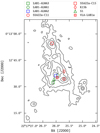 |
Fig. 1. Positions of confirmed galaxies within the LAB 1/LAB 8 structure (Table 1) shown alongside Lyα surface brightness contours from our MUSE adaptive narrow band image (see Sect. 5.2). The red circle and red square mark the Lyman Break Galaxies SSA22a-C11 and SSA22a-C15 from Steidel et al. (2003), respectively. The green circle and blue square mark the ALMA 850 μm detections LAB1-ALMA1 and LAB1-ALMA2 (Geach et al. 2016; Umehata et al. 2017), respectively. The red cross marks the position of the 3 GHz radio-continuum detection VLA-LAB1a (Ao et al. 2017). The red diamond indicates the K-band selected and spectroscopically confirmed galaxy LAB01-K15b from Kubo et al. (2015, 2016). The green square marks the ALMA 850 μm plus [C II] 158 μm detected source (Geach et al. 2016; Umehata et al. 2017). This source is also detected at 3 GHz with the VLA (S10 cm = 7.3 μJy; Ao et al. 2017) and it has a tentative X-Ray counterpart in the 400 ks deep Chandra data from Lehmer et al. (2009b). The serendipitously found z = 3.1 [O III] emitter S1 from Geach et al. (2016) is marked with a green triangle. The symbols used to indicate the embedded galaxies within the blob is used throughout the paper. North is to the top and east is to the left. The contours correspond to Lyα surface-brightness levels SBLyα = [200, 100, 50, 25, 8.75] × 10−19 erg s−1 cm−2 arcsec−2. |
Two of the Lyman-break galaxies from Steidel et al. (1998) are within the combined LAB 1/LAB 8 structure. Adopting the nomenclature of Steidel et al. (2003), these are SSA22a-C11 and SSA22a-C15. We list the coordinates of both galaxies in Table 11. SSA22a-C11 is located in the south-west of LAB 1, while SSA22a-C15 is found close to the Lyα photometric centre of LAB 8. Both galaxies have their redshift confirmed via near-IR detections of their [O III] λλ4963, 5007 lines (McLinden et al. 2013). Interestingly, McLinden et al. (2013) find no offset between Lyα emission line redshifts and [O III] redshifts. This is not commonly the case for high-z Lyα emitting galaxies where the Lyα line is typically found to be offset by ≳200 km s−1 with respect to the systemic redshift (e.g. Rakic et al. 2011; Chonis et al. 2013; Trainor et al. 2015). Since positive Lyα redshift offsets are usually interpreted as signs of outflowing expanding gas, McLinden et al. (2013) argue that C11 and C15 have no such prominent outflows. Moreover, C11 has an inferred star-formation rate of ≲10 M⊙ yr−1 (Steidel et al. 1998, 2003); thus this would fall short by more than a factor of ten in terms of producing the required amount of ionising photons to power LAB 1.
Overview of known sources within the Lyα blob.
Given the potential of obscured star-formation or AGN activity in the blob, it naturally became the target of several sub-mm and radio campaigns (Chapman et al. 2001, 2003; Matsuda et al. 2007; Yang et al. 2012; Geach et al. 2014, 2016; Umehata et al. 2017; Ao et al. 2017). Initial studies provided a confusing picture with purported detections by some that were vastly incommensurate with upper limits reached by others (see Sect. 2 of Geach et al. 2014). Nevertheless, advances in sub-mm detector technology and collecting area have led to a significant detection of three 850 μm sources within the blob (Geach et al. 2014, 2016; Umehata et al. 2017). Adopting the nomenclature of Umehata et al. (2017), these ALMA detected systems are denoted LAB1-ALMA1, LAB1-ALMA2, and LAB1-ALMA3. We list their coordinates in Table 1. LAB1-ALMA1 and LAB1-ALMA2 are in close vicinity to each other and close to the peak of Lyα surface brightness. LAB1-ALMA3 is located in the south-eastern part of LAB 1. The total measured 850 μm flux density from these three resolved ALMA sources is S850 μm = 1.7 mJy. This corresponds to star-formation rates of ∼150 M⊙ yr−1 under standard dust-heating assumptions. Moreover, hints for an extended low-surface brightness dust-component which is not detected by ALMA are seen in the fact that the single-dish SCUBA-2 observations (Geach et al. 2014) yield a factor of 2.7 higher flux compared to the interferometric measurement.
Ao et al. (2017) report 3 GHz radio-continuum detection slightly south of LAB 1-ALMA1 and LAB1-ALMA2. This S10 cm = 7.3 ± 2.2 μJy radio source is denoted VLA-LAB1a and we list its coordinates in Table 1. Given the proximity to LAB 1-ALMA1 and LAB1-ALMA2 the radio source is believed to be physically associated with the S850 μm ≈ 1 mJy sub-mm galaxies. According to Ao et al. (2017) the S850 μm/S10 cm ratio is atypical for a purely star-forming system and thus could be indicative of AGN activity. Both systems have no spectroscopic redshift confirmation independent of Lyα. However, sources at the positions of LAB1-ALMA1 and LAB1-ALMA2 are reported as K-Band selected galaxies with photometric redshifts in the range of 2.6 < z < 3.6 (Uchimoto et al. 2012, their Fig. 10).
LAB1-ALMA3 is spectroscopically confirmed as a [C II] 158 μm emitting source with ALMA (I[CII] = 16.8 ± 2.1 Jy km s−1, z[CII] = 3.0993 ± 0.0004; Umehata et al. 2017). It is also detected as a 3 GHz radio-continuum source with the VLA (S10 cm = 7.3 ± 2.2 μJy; Ao et al. 2017). As the coordinates of this radio counterpart are identical to those of LAB1-ALMA3, we do not list it as a separate source. Moreover, Ao et al. (2017) report a tentative X-Ray signal at the position of LAB1-ALMA3 using the deep (400 ks) Chandra full-band (0.5–8 keV) image from Lehmer et al. (2009b). Based on these observations, Ao et al. (2017) suggest the potential existence of an AGN in this source. Moreover, LAB1-ALMA3 appears as a K-Band selected galaxy in the sample of Uchimoto et al. (2012) and has been spectroscopically confirmed via Hβ and [OIII] λ5007 emission with MOIRCS on the Subaru telescope (Kubo et al. 2015, 2016). The redshift derived from those rest-frame optical lines (z = 3.1000 ± 0.004) is commensurate with the [C II]-based redshift.
Two more galaxies have been identified spectroscopically as members of the blob. LAB01-K15b is a K-Band-selected galaxy detected in [O III] emission (Kubo et al. 2015, 2016) and S1 is a serendipitous [O III] detection from Geach et al. (2016). The coordinates and redshifts of both sources were presented by Umehata et al. (2017) and are reproduced in Table 1. Lastly, Kubo et al. (2016) display a faint K-Band selected galaxy slightly south-west of SSA22a-C11 at a compatible photometric redshift (their Fig. 2), however, no coordinates for this potential member of LAB 1 are provided.
In summary, the LAB 1/LAB 8 system contains five spectroscopically confirmed galaxies. Guided by the systemic redshifts of the galaxies associated with the blob (Table 1), we fix z = 3.1 as its systemic redshift in the following. One of the spectroscopically confirmed systems, LAB1-ALMA3, is detected in 850 μm dust-continuum, [C II] 158 μm emission, 3 GHz radio continuum, and tentatively in X-Rays (Ao et al. 2017). Additionally, two 850 μm sources (LAB1-ALMA1 and LAB1-ALMA2) which are accompanied by a 3 GHz sources (VLA-LAB1a) are detected in the centre of LAB 1. While these sources are not spectroscopically confirmed members of the blob, their physical association with the system appears likely, especially given their prominent central position within the blob’s structure. To provide a visual overview of the with the LAB 1/LAB 8 system associated galaxies, we plot their positions with respect to the Lyα surface brightness contours in Fig. 1. For the latter, we make use of the MUSE data discussed in the remainder of the paper.
The interpretation that LAB1-ALMA1 and LAB1-ALMA2 are physically associated with the blob is further supported by results from imaging-polarimetry with FORS2 on the VLT by Hayes et al. (2011). The radial polarisation profile as well as the orientation of the polarisation vectors from those observations are consistent with predictions from Lyα radiative-transfer theory for Lyα scattering from a central Lyα powering source (Dijkstra & Loeb 2008). Interestingly, LAB1-ALMA1 and LAB1-ALMA2 are at the centre of the circular pattern denoted by the polarisation vectors from Hayes et al. (2011). More recent spectro-polarimetry with FORS2 by Beck et al. (2016) appears consistent with this scenario, although the interpretation of spectro-polarimetric Lyα data is more complex (Lee & Ahn 1998), as different scattering geometries and kinematics are degenerate with respect to observable polarisation signal (Eide et al. 2018). Especially, Trebitsch et al. (2016) challenged the interpretation of Hayes et al. (2011) by showing that the observed polarisation signal can be reproduced in a pure cooling-flow scenario. Thus, despite significant observational efforts and numerous counterpart identifications, there is still considerable debate regarding the mechanisms that power the Lyα emission of the blob.
Previous IFS observations of LAB 1 were obtained with the SAURON instrument at the WHT (Bower et al. 2004; Weijmans et al. 2010). These observations revealed a complex morpho-kinematic structure of the system in Lyα. The identification of multiple clump-like features in these data was seen as evidence for the presence of multiple galaxies in the system, while the chaotic motions were interpreted as signs of galaxy-galaxy interactions. Moreover, Weijmans et al. (2010) found signatures of coherent velocity shear at the positions of the Lyman-break galaxies C11 and C15. While these observations provided first insights into the complex kinematic structure of the system, they were limited in depth and spatial resolution. Here, we present the new deep MUSE observations of the system that allow us to map the spatial and kinematic structure of blob in unprecedented detail.
3. ESO VLT/MUSE Observations of LAB 1
LAB 1 was observed with MUSE (Bacon et al. 2010) in its wide field mode configuration without adaptive optics at the European Southern Observatories Unit Telescope 4 (Antu) in three service-mode programmes from 2014 to 2016 (ESO Programme IDs 094.A-0605, 095.A-0570, and 097.A-0831 with principal investigators Hayes, Bower, and Hayes, respectively). A log of these observations is given in Table 2. The individual exposure times are typically 1500 s, only with one exposure being significantly shorter (510 s). In total, the three programmes accumulated a total open-shutter time of 63390 s (17.6 h) on the target.
MUSE observations of LAB 1 present in the ESO archive.
The three different programmes centred the instrument on different regions of the blob. While programmes 094.A-0605 and 095.A-0570 centred the 1′ × 1′ MUSE field of view slightly north of LAB 1 to encompass also the northern neighbouring Lyα blob LAB 8, programme 097.A-0831 centred on a region south-west of the brightest blob structure. This offset was motivated by the detection of a previously unknown low-surface brightness extension of the blob in a reduction of the data from programme 094.A-0605 (see Geach et al. 2016). Each programme used the dithering and rotation pattern that is recommended in the MUSE observing manual2. Unfortunately, one exposure suffered from a severe tracking error and could not be used in the final analysis. Thus the total integration time of the analysable dataset is 17.2 h.
The DIMM seeing reported by ESO for the observation ranges from 0.5″ to 1.7″, but with the majority of exposures taken at sub-arcsecond seeing (mean: 0.87″, median: 0.88″). A potentially more accurate measurement of the seeing is provided by the FHWM measurements of stars in the meteorology fields recorded by MUSE’s slow-guiding system (SGS column of Table 2). Despite having a slightly larger scatter, the measured image quality by the SGS is often a bit better than the site-wide values provided by the DIMM (mean: 0.83″, median: 0.78″),
Programmes 094.A-0605 and 097.A-0831 were taken without the blue cut-off filter in the fore-optics (extended wavelength mode), thus allowing the wavelength range from 465 nm to 930 nm to be sampled (although at the cost of second-order contaminations at λ > 900 nm), while programme 095.A-0570 was taken with the blue cut-off filter within the light path (nominal wavelength mode), thus sampling the wavelength range from 480 nm to 930 nm.
All observational raw data and the associated calibration frames were retrieved from the ESO Science Archive Facility using the raw-data query form3 and the cal-selector tool. For all exposures, the associated calibration frames (bias frames, arc lamp frames, continuum lamp frames, twilight flats, standard star exposures, and astrometric standard fields) were taken as part of the standard calibration plan for MUSE observations. This means, in particular, that twilight flats were taken typically once a week, while standard-star exposures are usually obtained daily. Nevertheless, some retrieved exposures were associated to standard star4 exposure that were taken one night before or after the science observations.
4. Data reduction
4.1. Production of the datacube
For the reduction of the 17.6 h of MUSE observations into a science-ready datacube we used version 2.4.2 of the MUSE Instrument Pipeline (MUSE DRS – Weilbacher et al. 2016) provided by ESO5 and version 3.0 of the MUSE Python Data Analysis Framework (MPDAF – Bacon et al. 2016; Piqueras et al. 2017) provided by the MUSE consortium6. The MUSE DRS version used here incorporates the so-called self-calibration procedure to improve the flat-fielding accuracy for deep datasets (Conseil et al. 2016). For our data reduction, we adopted a similar strategy as the one used for the reduction of the MUSE Hubble Ultra Deep Field (Bacon et al. 2017).
We first ran the MUSE DRS calibration recipes muse_bias, muse_flat, muse_wavecal, and muse_lsf on the calibration frames that are associated to each science and standard star exposure. We also used the muse_twilight recipe on the twilight frames. Next, we applied the resulting calibration data products to each science and standard star exposure using the recipe muse_scibasic. The resulting standard-star pixtables were fed into muse_standard to create response curves, which were then applied to each science exposure with the muse_scipost task, using its self-calibration feature, but without using its sky-subtraction capabilities. When running muse_scipost, we used the associated astrometric calibrations provided from the ESO archive instead of the astrometric calibrations shipped with the pipeline. This approach was necessary, as the instrument underwent several interventions over the long period of observation. Not using the correct astrometric calibrations would result in uncorrected geometric distortions within the pixtables.
In order for self-calibration to work optimally, regions containing sources that are bright in the continuum needed to be masked. While in principle the DRS can automatically detect such regions, we manually masked out bright continuum objects a bit more conservatively compared to the DRS-generated mask. Manual masking was performed by visual inspection of the datacubes with the ds9 software (Joye et al. 2003) using polygon-shaped and circular regions. These regions were then converted into datacube masks using the pyregion python package7. Additionally, four science exposures contained continuum bright linear trails from moving objects (likely satellite flares, meteors or aeroplanes – affected exposures are marked by a † in Table 2). These trails were also masked manually for the self-calibration.
We then removed night sky-emission with muse_create_sky and muse_subtract_sky. During this step, we iteratively masked out regions that contained emission from the Lyα blob, so that the blob’s emission is not subtracted from the final data.
Next, we resampled the individual sky-subtracted and flux-calibrated exposure tables to the final 3D grid with muse_scipost_make_cube. We defined this final grid via an initial run of muse_expcombine on a subset of pointings from each observing programme. Using MPDAF’s combine method, we then produced an unweighted mean stack of those individual datacubes to produce the final science-ready datacube. Prior to this stacking, we masked out bright linear trails that were present in some observations (marked by a † in Table 2). We also ensured that remaining cosmic-ray residuals in the individual datacubes were filtered out in the final stack by using the κ-σ clipping algorithm in the combine task (two maximum iterations with σclip = 5).
The resulting final datacube has 456 × 378 spatial elements (spaxels) that sample the sky parallel to right ascension and declination at 0.2″ × 0.2″. Each spaxel consists of 3802 spectral elements that sample the spectral domain from 4599.6 Å to 9350.8 Å linearly with steps of 1.25 Å.
Throughout the above procedure, a formal variance propagation is also carried out by each of the used routines, thus a second datacube containing the variance for each volume pixel (voxel) is also produced. However, the resampling procedure in muse_scipost_make_cube produces correlated noise between neighbouring voxels (see Fig. 5 in Bacon et al. 2017). Since this co-variance term between neighbouring voxels cannot easily be accounted for in the final reduction, the formal variance cube contains underestimates of the true variances. By processing artificial pixtables filled only with Gaussian noise, Bacon et al. (2017) demonstrated that the variance for a voxel in an individual exposure datacube must be corrected by a factor of (1/0.6)2. Following Bacon et al. (2017), we applied this correction to our final variance cube.
We display a map of the integration time for each spaxel in the MUSE datacube of LAB1 in Fig. 2. The maximum integration time of 61920 s (17.2 h) is reached in a 32″ × 48″ central region of our datacube. In this region, all three ESO observing programmes overlap. This region completely encompassed the known extent of LAB 1 and LAB 8 prior to the observations presented here. Moreover, Fig. 2 also illustrates the location of the masked out regions due to continuum-bright meteor trails or satellite tracks.
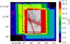 |
Fig. 2. Exposure map image for MUSE observations of LAB1 in the SSA22 field. The dashed rectangle indicates the zoomed-in region displayed in the spectral sequence shown in Fig. 3. Diagonal bands of lower exposure times are a result of masked out regions in the final cube stack due to contamination by bright satellite tracks or meteor trails in the individual exposures. To indicate the position and morphology of LAB 1 we also overlay the Lyα surface brightness contours from our MUSE adaptive narrow-band image (see Sect. 5.2). |
Lastly, we produce an emission line only datacube by subtracting a running median filter in spectral direction. This simple method for continuum removal has been proven effective in previous MUSE studies for isolating emission line signals (e.g. Borisova et al. 2016; Herenz & Wisotzki 2017; Herenz et al. 2017a,b; Arrigoni Battaia et al. 2019). Here we set the width of the median filter conservatively to 301 spectral layers (376.25 Å).
4.2. Astrometric alignment
We register the MUSE datacube to an absolute astrometric frame by using the 2MASS point-source catalogue (Skrutskie et al. 2006). Unfortunately, there are only two 2MASS sources within the limited FoV of the MUSE and STIS observations, with one of those sources actually being an extended galaxy. We therefore use the only real 2MASS point source (2MASS J22172397+0012359) to anchor our astrometric reference frame in both observational datasets.
By tying the astrometric reference frame only to one source, there still remain, in principle, several degrees of freedom with respect to geometrical distortions and rotation. However, rotation geometrical distortion are corrected for MUSE data at the pipeline level and the accuracy of this procedure is constantly monitored by ESO using astrometric calibration fields.
We verified our absolute astrometry against an archival HST/STIS 50CCD clear-filter image that is partially overlapping with our MUSE data (Proposal ID: 9174, presented and analysed in Chapman et al. 2001, 2004). We tied the absolute astrometry of this image also to the 2MASS point source. By visual inspection via blinking in ds9, we then ensured that no offsets exist between both datasets. We conservatively estimate that the absolute astrometric accuracy of our data to be on the order of one MUSE pixel (0.2″).
5. Analysis and results
5.1. Velocity sliced Lyα emission maps
We present a spectral sequence of pseudo-narrowband images over the Lyα line in Fig. 3. These images show that we can trace Lyα emission from LAB 1 over a bandwidth of ≈28 Å (±3000 km s−1 around zLy = 3.1). As can be seen from Fig. 3, the highest velocity gas emitting Lyα is located in the vicinity of the central sources LAB1-ALMA1, LAB1-ALMA2, and VLA-LAB1a. However, numerous other features with narrower spectral width appear only in a few velocity slices. Overall, the velocity slices reveal a complex spectral and morphological structure of Lyα emission throughout different parts of the blob. We label notable features in Fig. 3, where we indicate the following. (1) A circular structure devoid of strong Lyα emission towards the north of the sub-mm sources: this feature is labelled as a “bubble” in Fig. 3. It is most clearly seen in the slice around 4979 Å, where we indicate this feature with an arrow. In subsequent redder slices, this “bubble” appears with less contrast. It appears as if its radius increases from ∼20 kpc at 4979 Å to up to ∼40 kpc towards redder wavelengths. (2) A filamentary narrow bridge connecting LAB 1 to LAB 8 in the north: this bridge becomes visible in the slice at 4979 Å and can be clearly followed until the 4989 Å slice. For LAB 8, the flux shears from the north-west to the south-east with increasing wavelength and the filament shows the same velocity shearing. We indicate this by labelling it as “LAB1-8 bridge (blue arm)” and “LAB1-8 bridge (red arm)” of the bridge in the panel displaying the 4979 Å slice and 4989 Å slice, respectively. (3) A compact emission knot towards the north of LAB 8, which connects to LAB 8 via a faint low-surface brightness filament: this feature is seen in the slices at 4981.5 Å and 4984 Å, and we label it “LAE with filament” in the 4984 Å slice. This newly discovered LAE and filament is close to the edge of the field of view of the observations and, thus, only exposed at 8 h–12 h, so the noise in this part of the datacube is significantly larger. Nevertheless, as we discuss in the following Sect. 5.4, the compact emitter and the filament are significant detections. (4) A faint extended, slightly curved, shell-like region towards the south-west of LAB 1: along the major axis, the extent of the shell is ∼120 kpc and its projected thickness is ∼30 kpc. This low-surface brightness emission is visible in the slices from 4976.5 Å to 4981.5 Å, where we label it simply as a “shell”. The shell region appears to be connected to the main area of LAB 1 via a low-surface brightness filament trailing from the north-east to the south-west. The filament is most prominently visible in the 4981.5Å slice, where we label it a “shell connecting filament”. In the northern part of this shell-like region, a compact high-surface brightness knot is visible. This knot is accompanied by another slightly more diffuse knot. These two knots in the northern part of the shell can be traced in the velocity slices from 4974Å to 4981.5Å, and we label both features as “2 knots” in the 4974Å slice. (5) Another compact isolated Lyα line emitter towards the south-east of LAB 1 is seen in the slices from 4984 Å to 4989 Å. We show in the following, namely, in Sect. 5.2, that this emitter is one of four newly detected Lyα emitters in the proximity of the LAB 1/LAB 8. We label this emitter “LAE” in the 4984Å slice.
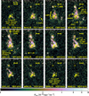 |
Fig. 3. Spectral sequence of pseudo-narrowband images of LAB 1 from 4971.5 Å to 4999.0 Å created from the continuum subtracted MUSE datacube. Each image has a band-width of 2.5 Å and in order to enhance low-surface brightness features the images have been smoothed with a σ = 1 px (0.2″) Gaussian kernel. In each panel, we indicate the positions of known galaxies within the blob (see Sect. 2 and Fig. 1). Moreover, we show in each panel a scale that indicates 50 kpc in projection at z = 3.1 (6.49″). The morphological features described in Sect. 5.1 are indicated in the bluest image where they become visible. We also indicate that we trace Lyα emission ±3000 km s−1 around the central sources of LAB 1. North is up and east is to the left. |
A closer inspection of the velocity slices reveals that there appears to be an overall velocity shear. The bluer v < 0 km s−1 slices show predominantly emission towards the west, while the redder v > 0 km s−1 slices are dominated by emission from the east. This structure of the velocity shear becomes more clear in our moment-based analysis of the Lyα line profiles (Sect. 5.3).
5.2. Detection and photometric measurements of Lyα emission
5.2.1. Method
To determine the overall Lyα surface-brightness morphology of LAB 1 from our MUSE datacube, it would not be optimal to create a simple narrow-band image by summing over a certain number of datacube layers. Choosing a single bandwidth for such an image would either decrease the signal-to-noise ratio (S/N) for regions where the Lyα profiles are very broad if the bandwidth that is chosen too narrow; or, conversely, decrease the S/N in regions where Lyα is narrow if the adopted bandwidth would optimally encompass the broader profiles. Furthermore, such a simple summation would not account for the presence of velocity shear. Thus, we create an adaptive narrow-band image. For this image, we sum only over voxels that contain Lyα flux. Our method is similar to the creation of the narrow-band images in the analysis of extended Lyα emission around QSOs from MUSE data (e.g. Borisova et al. 2016; Arrigoni Battaia et al. 2019).
In order to find the spectral pixels over which we need to sum, we utilised the 3D cross-correlation procedure of the LSDCat software8 (Herenz & Wisotzki 2017). The LSDCat software produces an S/N datacube by cross-correlating the continuum subtracted datacube with a 3D Gaussian template. The parameters of the template are the amount of spatial and spectral dispersion of the 3D Gaussian. Cross-correlation suppresses high-frequency noise while maximising the S/N of signals within the data that match the template. Hence, the method is commonly called “matched filtering” (e.g. Vio & Andreani 2016; Loomis et al. 2018).
LSDCat was originally developed for the detection of Lyα emitting galaxies in blind MUSE surveys (see Herenz et al. 2017b; Urrutia et al. 2019). For this application, the parameters of the template are optimally chosen when they match the width of the seeing point spread function (PSF) and the average line width of LAEs (see Sects. 4.2 and 4.3 in Herenz & Wisotzki 2017). However, our goal here is not to optimise the template for compact emission line sources, but to maximise the detectability of faint low-surface brightness filaments in the outskirts of the blob. Simultaneously, we want to preserve the morphology of small-scale surface-brightness variations. As there is no optimal a priori solution to this problem, the final set of adopted parameters had to be chosen by parameter variation and visual inspection of the resulting images. By experimenting with different spatial filter widths, we found that a spatial full width at half medium (FWHM) of 1.8″ preserved most of the contrast of compact features and significantly enhanced the S/N of the extended filamentary features in the outskirts of the blob. The adopted filter FWHM is roughly twice the seeing PSF FWHM9 of 0.95″. As derived by Zackay & Ofek (2017), a filter width of twice of the seeing FWHM reduces10 the maximum S/N of compact sources only by 20%. Similarly, we varied the FWHM of the spectral part and found that 300 km s−1 is well suited for enhancing the detectability of the blob’s low-surface brightness features.
5.2.2. Maximum S/N image
In Fig. 4, we show the resulting map when taking the maximum S/N in from the LSDCat S/N datacube around zLyα = 3.1. We adopt an S/N threshold of six as a detection threshold to identify reliable regions from which Lyα emission is detectable. These regions are demarcated by a white dashed line in Fig. 4. An S/N threshold of six has previously been proven effective to maximise the ratio of real- to spurious detections in blind emission line searches with MUSE (Herenz & Wisotzki 2017; Herenz et al. 2017b; Urrutia et al. 2019). This is also visualised in Fig. 4, where we include spaxels in the display down to a S/N of four. Inspecting spectra extracted in the 4 < S/N < 6 regions revealed that in all those cases, a possible emission line signature is at most marginal, while the S/N > 6 regions are confident detections.
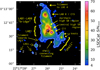 |
Fig. 4. Map of the maximum signal-to-noise ratio (S/N) after cross-correlating the datacube with a 3D Gaussian template (see Sect. 5.2 for details on the construction of this image). Pixels with S/Nmax < 4 and contaminating foreground sources are masked (regions in black). Thus, pixels shown in colour are a 2D projection of the 3D mask utilised to construct the adaptive narrow band image displayed in Fig. 5. The dashed contour demarcates region of connected pixels with S/Nmax ≥ 6. This highlights that LAB 1, LAB 8 and the newly detected shell comprise a significantly detected contiguous region. The four enumerated features in this image are regions that contain pixels with S/Nmax ≥ 6 that have no pixel connectivity at S/Nmax ≥ 6 with the LAB1/LAB8 + shell structure; these detections are LAEs in the vicinity of the blob and are further discussed in Sect. 5.4. Previously known galaxies at z = 3.1 are indicated using the symbols in Fig. 1 and interesting features are annotated. |
While our goal is to use the S/N datacube from the 3D cross-correlation as a mask to produce an optimally extracted narrow-band image, its 2D representation in the form of maximum S/N map in Fig. 4 provides us with a schematic visualisation of the main morphological features of the system. We annotate these in Fig. 4. Most of the features were already hinted at in the display of the velocity slices in Fig. 3.
Marked S/N peaks are found at the position of the LBG SSA22a-C11 in LAB 1 and near the LBG SSA22a-C15 in LAB 8. We point out that the LAB 8 peak shows a slight offset towards the south of SSA22a-C15. The centre of LAB 1 shows an extended region of high S/N, that exhibits its peak values at LAB1-ALMA2. This area is labelled “central high SB region” in Fig. 4. Interestingly, the sub-mm, [CII] and potentially X-Ray-detected source LAB1-ALMA3 do not have an associated prominent peak in the S/N map, and neither have the spectroscopically confirmed sources S1 and K15b associated peaks. However, these three sources (LAB1-ALMA3, S1, and K15b) demarcate the central high surface-brightness region from the south-east (LAB1-ALMA3, S1) to the north-west (K15b). In the north-west, another high surface-brightness region then curves back to the north-east. This feature is labelled “northern high surface-brightness region” in Fig. 4 and does not contain known sources. It is, however, spatially coincident with the northern edge of the “bubble” that we pointed out in Sect. 5.1 (see Fig. 3).
Our maximum S/N map also accentuates the two filamentary features that form a bridge between LAB 1 and LAB 8. Moreover, the newly detected “shell” region in the south west is clearly connected via a significantly detected filament to the central region of the blob. This shell harbours a compact high-S/N knot, accompanied by more diffuse emission knots towards the north and the south. We also find four isolated S/N > 6 peaks (labelled 1 to 4 in the figure) that are not connected to the central large S/N > 6 region. These isolated S/N > 6 peaks represent newly identified Lyα emitters in close vicinity to the blob and they are analysed separately in Sect. 5.4. With regard to LAE 4 to the north of LAB 8, it appears to be connected by a filamentary structure to the main body of the blob, but this potential filament is detected at lower significance than our adopted detection threshold. The map also hints a potential filament pointing towards LAE 3.
5.2.3. Adaptive narrow-band image
Equipped with the S/N datacube from LSDCat, we constructed the optimal 3D extraction mask for our adaptive narrow-band image. We do so by summing the flux datacube in the spectral direction only over voxels that contain at least an S/N value above four in the S/N datacube. We note that spaxels that do not contain a single voxel with S/N > 4 are blacked out in Fig. 4, thus the displayed spaxels in Fig. 4 can be interpreted as a 2D projection of the 3D extraction mask. The choice of this analysis threshold is motivated by our observation that some S/N > 4 regions in Fig. 4 may contain a marginal Lyα signal. The use of a second S/N threshold that is lower than the detection threshold is also core principle of the LSDCat software, which uses a detection threshold for finding emission lines and an analysis threshold for performing measurements on the detected lines (Herenz & Wisotzki 2017). In order to provide a visual representation of the background noise in source-free regions, we adopt the strategy from Borisova et al. (2016) and sum over four spectral bins. We centre the summation around 4983.4 Å (the wavelength of Lyα at z = 3.1). The adaptive narrow-band image constructed in this way is displayed in Fig. 5. The 1σ noise of the image estimated from placing random apertures in empty sky regions in the central parts of the image is 4 × 10⁻²⁰ erg s−1 cm−2 arcsec−2.
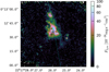 |
Fig. 5. Adaptive narrow-band image of LAB1. The image is the result of summing only over voxels in the continuum-subtracted datacube that have a S/N > 4 in the LSDCat cross-correlated datacube. For spaxels that do not contain voxels above this threshold we simply sum over 5 Å (four datacube layers) around 4985.6 Å (=(1 + zLAB1) × λLyα). As in Fig. 4, we masked sources where the continuum subtraction with a running median filter failed. In order to further enhance low-SB Lyα features, we smoothed the final image with a σ = 0.2″ Gaussian kernel. The photometric centre and the principal axis of the blob are indicated by a cyan cross and a cyan dashed line, respectively. Previously known galaxies at z = 3.1 are indicated using the same symbols as in Fig. 1. |
The adaptive narrow-band image allows us to characterise the features that were pointed out above (Figs. 3 and 4) by Lyα surface brightness11 (SBLyα). We distinguish three fragments in the shell: (1) A bright compact knot with SBLyα ≈ 5 × 10⁻¹⁸ erg s−1 cm−2 arcsec−2; (2) a fainter, more diffuse knot to the north of the bright knot with SBLyα ≈ 2.8 × 10⁻¹⁸ erg s−1 cm−2 arcsec−2; and (3) an even more diffuse extended fragment in the south of the shell with SBLyα ≈ 1.6 × 10⁻¹⁸ erg s−1 cm−2 arcsec−2. The filament connecting the diffuse part of the shell (labelled as shell-connecting filament in Fig. 5) is characterised by SBLyα ≈ 1 × 10⁻¹⁸ erg s−1 cm−2 arcsec−2 emission, while the central- and northern high-surface brightness regions of LAB 1 show SBLyα ≳ 1 × 10⁻¹⁷ erg s−1 cm−2 arcsec−2. The high-SBLyα regions clearly demarcate a central circular region of lower SBLyα (SBLyα ≈ 5 × 10⁻¹⁸ erg s−1 cm−2 arcsec−2). This apparent cavity, first seen by Bower et al. (2004), was labelled “bubble” in Fig. 3. To the north of LAB 1 we find the two filaments connecting LAB 1 with LAB 8, with the eastern one showing higher SBLyα (SBLyα ≈ 4.5 × 10⁻¹⁸ erg s−1 cm−2 arcsec−2) than the western one (SBLyα ≈ 2.5 × 10⁻¹⁸ erg s−1 cm−2 arcsec−2). LAB 8 is characterised by SBLyα ≳ 1 × 10⁻¹⁷ erg s−1 cm−2 arcsec−2 and for the filament towards LAE 4 in the north, we measure SBLyα ≈ 1 × 10⁻¹⁸ erg s−1 cm−2 arcsec−2. However, in the northern part of the image, due to the lower number of contributing exposures (see Fig. 2), the background noise of the image is higher (σ ≈ 6 × 10⁻²⁰ erg s−1 cm−2 arcsec−2). With S/Nmax values ∼5−5.5 after the 3D cross-correlation procedure, it misses the adopted detection threshold and we regard this filament conservatively only as a tentative feature.
5.2.4. Size and total Lyα luminosity
We define the size of the unveiled LAB 1 + LAB 8 + shell structure as the area of the region above the adopted detection threshold of S/Nmax = 6 (white contour in Fig. 4), excluding the isolated LAEs. In terms of surface brightness this threshold corresponds to a limit of ≈6 × 10⁻¹⁹ erg s−1 cm−2 arcsec−2. The corresponding limit in surface luminosity is 8.7 × 1038 erg s−1 kpc−2. At this threshold, Lyα emission from the LAB 1/LAB 8 structures covers an area of 553 arcsec2. This corresponds to a projected surface of 3.2 × 10⁴ kpc2 at z = 3.1. The total measured Lyα flux from the structure is FLyα = 1.73 × 10⁻¹⁵ erg s−1 cm−2, which corresponds to a Lyα luminosity of LLyα = 1.45 × 1044 erg s−1.
While the Lyα structure revealed here is enormous, two even larger Lyα nebulae, namely the “Slug” nebulae, with an extent of ≈500 kpc (Cantalupo et al. 2014), and the MAMMOTH-1 nebula, with an extent of ≈440 kpc (Cai et al. 2017), are known. While the “Slug” nebulae surrounds a luminous (Lbol = 1047.3 erg s−1) type-I quasar, the MAMMOTH-1 nebulae surrounds a relatively faint broad-band source whose emission line spectrum appears to be consistent with a quasar. Nevertheless, both the “Slug” and the MAMMOTH-1 nebulae are also characterised by a factor of 3.4 and 1.5 higher luminosity than the LAB 1 + LAB 8 + shell structure, respectively. Both nebulae are at z ≈ 2.3 and, thus, the effect of cosmological surface brightness dimming is reduced by a factor of 2.4 compared to our observations. While no limiting surface brightness for the “Slug” observations has been published, Cai et al. (2017) report a surface brightness detection limit of 4.8 × 10⁻¹⁸ erg s−1 cm−2 arcsec−2 for MAMMOTH-1. This translates to limiting surface luminosity of 6.8 × 1038 erg s−1 kpc−2, which is comparable to our physical limit. The projected maximum extend of our structure, measured from the northernmost tip in LAB 8 to the southernmost point in the shell, is 45.4″ or, correspondingly, 346.3 kpc in projection, which is a factor of ≈0.8 smaller that the extent of the MAMMOTH-1 nebula. Similarly to the LAB 1 – LAB 8 structure, MAMMOTH-1 exists in an extreme overdense region of the universe.
5.2.5. Photometric centre and photometric principal axis
We applied the formalism of image moments (Hu 1962; Stobie et al. 1980; Stobie 1986) to the adaptive narrow-band image to calculate the photometric centre as well as the angle of the principal axis, θPA, of the LAB. In pixel-coordinates (x, y) of the adaptive narrow-band image Ixy the photometric centre  is defined as
 (1)
(1)
and the angle of the principal axis is defined as
 (2)
(2)
with
 (3)
(3)
and
 (4)
(4)
For these calculations, we only considered pixels in the narrowband image Ixy that have a corresponding pixel above a S/N of six in the maximum S/N map. Moreover, the definition of the angle of the principal axis in Eq. (2) is such that 0° corresponds to the axis from S to N, and that the angle increases counterclockwise to the east. The photometric centre obtained in this way and converted to celestial coordinates (J2000), is located at RA = 22h17m25.94s, Dec = +00°12′39.338″, and for the angle of the principal axis, we find θPA = 20.9° east of north.
We show the position of the photometric centre in Fig. 5 by a cyan cross. As can be seen, the photometric centre is located slightly west to the “bubble”. We also indicate the principal axis in Fig. 5 by a dashed cyan line. Figuratively speaking, the principal axis is the axis along which the blob appears most elongated. Formally, it describes axis along which the variance in flux is maximised. For a light distribution of elliptical shape, the so defined principal axis would be oriented along the major axis of the ellipse. Thus, our θPA measurement is comparable to the measurements of LAB position angles via ellipse fitting in Erb et al. (2011). We discuss the alignment between principal axis and gas kinematics in Sect. 6.3.1.
5.3. Moment based maps of the Lyα line profile
By visually inspecting the Lyα spectral profile as a function of position with the QFitsView software12 (Davies et al. 2010; Ott 2012), we find that the line profile complexity varies strongly throughout the blob. We illustrate this by showing a selection of representative profiles in Fig. 6. As shown, in some regions, the profiles appear very broad and with a dominating peak (e.g. panel 12 in Fig. 6), while other regions are characterised by clearly double (e.g. panel 3) or even multi-component profiles (e.g. panel 5 or panel 9). The isolated LAEs in the outskirts (example in panel 4, see also Fig. 9) or in the shell-like region (panel 7) show narrower Lyα profiles.
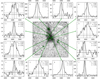 |
Fig. 6. Examples of the variety and complexity of the Lyα line profiles encountered in LAB 1. All profiles are extracted in circular apertures of 1.2″ diameter, except for LAB 8, where a 4″ diameter aperture was used. The image in the centre is the adaptive narrow-band image shown in Fig. 5, but in a logarithmic scale. Green circles represent the extraction apertures with lines connecting to the individual panels that display the profiles. Four of the twelve panels show Lyα profiles at the position of known galaxies: LAB1-ALMA3 in panel 5, SSA22a-C11 in panel 6, LAB1-ALMA1 and LAB1-ALMA2 in panel 9, and SSA22a-C15 (LAB 8) in panel 12. For each profile, the wavelength axis (in Å) is fixed and centred on zLyα = 3.1, but the axis displaying the intensity (in erg s−1 cm−2 Å−1) is scaled to encompass the maximum flux value of each profile. We also indicate in each panel the flux-weighted central moment (Eq. (5), dashed line), and the non-parametric measure for the width of the line obtained from the second flux-weighted moment (from Eq. (6) with k = 2, dotted lines). Moreover, we display in the upper right corner of each panel the non-parametric descriptive measures skewness s (Eq. (10)), kurtosis κ (Eq. (11)), and bi-modality b (Eq. (12)) – see text for details. All non-parametric descriptive statistics are computed by considering only the range of connected positive spectral bins blue- and red-wards of the peak. |
The varying complexity of the Lyα profiles as a function of position prohibit parametric fits of a simple model to the spaxels of the datacube in order to create maps of, for example, the velocity centroid (vr) or line-width (σv). Such an analysis was presented for the much shallower SAURON data of LAB 1 (Bower et al. 2004; Weijmans et al. 2010), but the increased sensitivity and resolution of our MUSE data warrant a different approach. We thus resorted to a moment-based non-parametric analysis. Our method is rooted in descriptive statistics (e.g. Ivezić et al. 2014), but we needed to account for two differences when describing spectroscopic line profiles instead of statistical data with such an ansatz. First, the formal validity of the summarising parameters is only given when positive values are considered in the calculations. Second, the presence of noise and the usage of small sets of input values can lead to non-trivial biases in moment-based quantities, especially if the analysed profiles are of low S/N. To ensure positive values and in order to minimise low-S/N biases we first applied three preprocessing steps to the continuum-subtracted datacube: Firstly, we used the 3D mask that was already used for the creation of the adaptive narrow band image in Sect. 5.2.2. We recall that this 3D mask was constructed by thresholding the matched-filtered datacube with S/N > 4. Voxels that do not fulfil this criterion are set to 0 in the analysis. Secondly, we smoothed each layer of the flux datacube with a circular 2D Gaussian (σ 0.8″). This is done to reduce the spaxel-to-spaxel noise in the final maps, especially in low surface-brightness regions. This value significantly improved the S/N ratio of the Lyα profiles in the filaments and low surface-brightness regions of the blob. Lastly, we used a 2D mask by thresholding the maximum S/N map shown in Fig. 4 to exclude spaxels were only a very small number of spectral bins would contribute to the resulting moments. After visual inspection we set this “display threshold” to S/Nmax = 6, that is, the analysed regions are exactly the regions that we regarded as confident detections in Sect. 5.2.2. After these preparatory steps, we created a 2D array of the central flux-weighted moment (first moment) from the processed datacube voxels Fxyz,
 (5)
(5)
as well as 2D arrays  of the kth flux-weighted moments,
 (6)
(6)
for k = 2, k = 3 and k = 4. In Eqs. (5) and (6), as well as in the following equations below, x and y denote the indices of spatial axes of the flux datacube F, while z indexes the spectral direction.
The first moment map resulting from Eq. (5) directly translates into a line-of-sight velocity map
 (7)
(7)
where c is the speed of light,  is the non-linear translation between MUSE spectral pixel coordinate and vacuum wavelength13 and zLAB1 is the systemic redshift of LAB 1. For this translation, we fix the systemic redshift of LAB 1 to zLAB1 = 3.1, which is in agreement with known redshifts of the galaxies within the blob. The so created
  map is shown in the left panel of Fig. 7. There we also show the photometric centre and the principal axis that were computed from the adaptive narrow band image as described in the previous section. We point out that the principal axis is oriented orthogonal to the direction of the apparent large-scale velocity gradient. This feature is further discussed in Sect. 6.3.
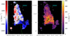 |
Fig. 7. Apparent line-of-sight-velocity (left panel) and apparent velocity dispersion (right panel) as measured from Lyα using the first and second flux weighted moments (Eqs. (7) and (8)). Before the moment-based analysis was carried out, each layer of the datacube was spatially smoothed with a σ = 0.8″ Gaussian kernel. In each spaxel, only spectral bins above a S/N threshold of four in the LSDCat S/N datacube were used in the summations in Eqs. (5) and (6). Moreover, the displayed map shows only spaxels that have a maximum S/N > 6. Thin grey contours indicate surface-brightness levels SBLyα = [200, 100, 50, 25, 8.75] × 10−19 erg s−1 cm−2 arcsec−2 as measured in the adaptive narrow-band image (Fig. 5). The positions of confirmed galaxies within the blob are indicated with the same symbols as in Fig. 1. The photometric centre and the principal axis of the blob (see Sect. 5.2 and Fig. 5) are indicated by a green cross and a green dashed line, respectively. The horizontal cyan line in the upper right of each panel indicates a projected proper distance of 50 kpc. |
By taking the square root of second moment map (Eq. (6), with k = 2) we compute a map that provides a measure of the width of the spectral profiles:
 (8)
(8)
This σv map is shown in the right panel of Fig. 7. We express the width of the profiles σv in km s−1, but caution that this measurement cannot be directly interpreted as velocity dispersion as it is often done for non-resonant emission lines. For example, double- or multiple-peaked profiles generally have larger second moments than single-peaked profiles. Moreover, radiative transfer effects are also known to broaden the single-peaked Lyα line profiles when compared to non-resonant emission lines (see also Sect. 5.5). We thus call the second moment based measure “apparent velocity dispersion”. Lastly, the spectral resolution of MUSE also has an effect on the apparent velocity dispersion. Given the complexity of the profiles and the non-parametric nature of our measurement, the effect of broadening the profiles via convolution with the spectrograph’s line-spread function (LSF) is not easily quantifiable. The measured instrumental width for MUSE at 4980Å is σinst ≈ 75 km s−1 (Bacon et al. 2017). As a figure of merit estimate, this translates into resolution corrections, σcorr, of −34 km s−1, −20 km s−1, −15 km s−1, and −10 km s−1 for apparent velocity dispersions of 100 km s−1, 150 km s−1, 200 km s−1, and 300 km s−1, respectively, if the observed line profiles and the line spread function are well approximated by a Gaussian profile, that is,
 (9)
(9)
Creating such moment-based maps of line-of-sight velocity and apparent velocity dispersion is common in the analysis of synthesised datacubes from radio-interferometric 21 cm observations of galaxies (e.g. Thompson et al. 2017, Section 10.5.4). It now is also routinely used in the analyses of extended Lyα nebulae surrounding quasars (e.g. Borisova et al. 2016; Arrigoni Battaia et al. 2018, 2019; Drake et al. 2019). Moreover, recent theoretical works by Remolina-Gutiérrez & Forero-Romero (2019) and Smith et al. (2019) resort on a moment-based analysis in the analysis of Lyα profiles from Lyα radiative transfer simulations. However, in order to create maps that characterise the varying complexity of the Lyα profile as a function of position in the blob, we use measurements involving higher-moments. Remolina-Gutiérrez & Forero-Romero (2019) suggest using the skewness, s, the kurtosis, κ, and the bimodality, b. These measurements are detailed in the following. To provide a visual guide on how to interpret these quantities, we also display their values next to the example profiles from the blob shown in Fig. 6.
We calculate a map of the Lyα profile skewness s via
 (10)
(10)
The skewness defined in this way (−1 ≤ s ≤ 1) quantifies the asymmetry of the spectral profile with respect to m1. If s ≃ 0 the profile is symmetric around m1 (panel 1 in Fig. 6), while for s > 0 a tail is found redwards of m1 (e.g. panels 4 and 11 in Fig. 6) and for s < 0 a tail is bluewards of m1 (e.g. panels 6, 8, and 10 in Fig. 6). We show our computed map for sxy in the left panel of Fig. 8.
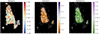 |
Fig. 8. Maps of higher moment-based non-parametric measurements for visualising the varying complexity of the Lyα profiles throughout the blob. We show maps of skewness s (left panel), kurtosis κ (centre panel), and bimodality b (right panel), as defined in Eqs. (10)–(12), respectively (see text for details). The displayed map in the left panel (middle and right panel) shows only spaxels that have a maximum S/N > 6 (maximum S/N > 13). Skewness s quantifies the asymmetry around the first central moment m1 (Eq. (5)), with s = 0 (yellow) indicating symmetric profiles, while s < 0 (shades of blue) indicate that the profile shows a larger tail towards the blue and s > 0 (shades of red) indicate that the profiles show a larger tail towards the red. Kurtosis quantifies the strength of wings (symmetric profiles) or tails (asymmetric profiles), with κ = 3 (white) indicating that the wings of the profile are comparable to a Gaussian wings, while κ > 3 (shades of purple) indicate larger tail extremity of the profiles (shades of brown), and κ < 3 indicate that there is less power in the tails compared to a Gaussian. Bimodality b is an attempt to quantify whether the profiles are double-component (b ≲ 2.6, green colours) or single-component (b ≳ 3, shown in violet) profiles (Remolina-Gutiérrez & Forero-Romero 2019). However, given the presence of noise and finite spectral resolution, a clear discriminatory power between single-component and double-component is not given by this measure in range 2.6 ≲ b ≲ 3 (light green and light violet colours). Contours and symbols are the same as in Fig. 7. |
We note that definitions other than Eq. (10) have been used in the literature to quantify the asymmetric Lyα line-profile morphology of LAEs. For example, Shimasaku et al. (2006) quantified the observed skewness in spectral profiles from Lyman α emitting galaxies by multiplying the definition given in Eq. (10) with a measure of the width of the line; however, we prefer to not entangle those two quantities. Other authors (Mallery et al. 2012; U et al. 2015) have quantified skewness s by fitting a skewed Gaussian profile. Yet this approach does not capture the complex Lyα spectral profiles seen here in LAB 1. Additionally, Childs & Stanway (2018) recently showed that the skewness values derived from fitting an asymmetric Gaussian do not accurately capture the true skewness of Lyα profiles in the presence of finite spectral resolution and background noise. Two other alternative definitions have been put forward by Dawson et al. (2007). These authors quantify asymmetry either via the ratio of flux blue- and redwards of the peak or via the ratio of the widths than encompass 90% of the flux blue- and redwards of the peak. However, given that the profiles in LAB 1 sometimes show multiple peaks at substantial spectral distance (e.g. panels 1 and 3 in Fig. 6), quantifying asymmetry around the higher peak would exaggerate the skew measure compared to the visual perception of symmetry in those profiles.
We obtain a map of the kurtosis of the Lyα profiles via
 (11)
(11)
Kurtosis quantifies how much flux is in the wings of the profiles in comparison to the wings of Gaussian profile (i.e. their tail extremity). For κ = 3, the tails are comparable to the Gaussian profile, while profiles with κ > 3 show more pronounced tails (e.g. panels 6 and 11 in Fig. 6), while κ < 3 indicates the absence of pronounced tails (e.g. panels 1, 5, and 9 in Fig. 6). Of course, only wings that are significantly above the noise can contribute to this statistic. As a corollary, regions of low S/N are biased towards to low kurtosis values. We avoid these biases by increasing the display threshold to S/Nmax = 13. We show the resulting map for κxy in the centre panel of Fig. 8.
Following Remolina-Gutiérrez & Forero-Romero (2019) we calculate a map of the bi-modality of the Lyα line profiles using
 (12)
(12)
Remolina-Gutiérrez & Forero-Romero (2019) introduced this quantity to discriminate whether their Lyα radiative transfer models result in single- or double component profiles. We point out that this measure is not a formal statistical test for bi-modality, but it can capture the visual appearance of the Lyα profile morphologies. We find that for b ≲ 2.6 profiles appear mostly to have clearly distinct double component structures (e.g. panels 1 and 4 in Fig. 6, but also see panel 5 and 9), while profiles with b ≳ 3 appear single peaked (e.g. panel 2, 6, and 7 in Fig. 6). However, some b ≳ 3 profiles may also have a subdominant second component, that is mainly contributing to the kurtosis (e.g. panel 11 in Fig. 6). In the range 2.6 ≲ b ≲ 3, however, the discriminatory power of b appears not strong, and visual inspection of those profiles indicates a high complexity with possible multiple components or peaks (see e.g. panels 3 and 10 in Fig. 6). Despite its potential lack of accuracy, qualitatively b captures the visual complexity of the profiles, with higher values indicating simple single component profiles and lower values indicating more complex profiles, and with the lowest values often corresponding to the presence of double component profiles. Moreover, since the κ is biased towards low values in regions of low S/N, also b is biased low in those regions. Thus, we hide the biased regions by setting the display threshold to S/Nmax = 13. We show our computed map for bxy in the right panel of Fig. 8.
It can be seen that most of the blob shows low values of b indicative of double component Lyα profiles. This impression is also on par with our visual inspection of the line profile variations throughout the blob. Moreover, in the central high surface-brightness region of LAB, where also the broadest profiles are observed, we obtain b values in the intermediate range – these profiles often appear to exhibit a high-degree of complexity. Lastly, only a few small island regions can be characterised by high values of b. These regions show clearly distinct single peaked profiles, often with very pronounced tails. The maps derived and presented here from the moment-based analysis are discussed in Sect. 6.3.
5.4. Newly discovered faint LAEs at z ≈ 3.1 in proximity to LAB 1
As mentioned in Sect. 5.2, our S/N map revealed four detections that are not embedded in the extended Lyα radiation from the blob. We labelled those sources 1 – 4 in Fig. 4. These sources are detected with S/N > 6 in the LSDCat cross-correlated datacube. Formally, one more detection with S/N > 6 at z = 3.1 exists close to the eastern border of Fig. 4, however this detection turned out to be an artefact near the edge of our field of view.
The coordinates, Kron-radii, and fluxes of the newly detected LAEs are listed in Table 3. These measurements have been obtained with the LSDCat software (Herenz & Wisotzki 2017). In Fig. 9, we show the spectral profiles of the detections. These 1D spectra have been extracted within a circular aperture of radius Rkron. No other lines are detected at these positions and thus we are confident that the sources are LAEs in physical proximity to the blob. Additionally, two of the line-profiles (LAE 3 & LAE 4) are reminiscent of the characteristic red-asymmetric line-profiles seen typically in LAEs (e.g. Dawson et al. 2007; Yamada et al. 2012). At z = 3.1 the range of the measured fluxes is log FLyα[erg s−1cm−2] = −17.2…−16.6, which corresponds to Lyα luminosities log LLyα[erg s−1] =41.7…42.3. Hence, those galaxies occupy the faint-end ( ) of the LAE luminosity function (Drake et al. 2017a,b; Herenz et al. 2019) and, thus, they are below the detection limit of classical narrow-band imaging surveys.
Newly detected faint z = 3.1 LAEs around LAB1.
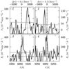 |
Fig. 9. Spectral profiles of the newly discovered LAEs 1 – 4 (as labelled in Fig. 4, clockwise from top-left to bottom-right). Spectra (black lines) have been extracted within a circular aperture of radius Rkron (see Table 3). The propagated error spectrum from the variance cube in this aperture is shown as a grey line. The vertical dashed line indicates zLyα = 3.1, whereas the vertical dotted lines indicate the measured redshifts from the profiles (see Table 3). |
From the spectral profiles we measure the LAEs redshifts using the first flux-weighted moment (Eq. (5)). These redshifts are indicated as a vertical dotted lines in Fig. 9. We list the velocity difference Δv with respect to z = 3.1 in Table 3. The two galaxies, 1 and 3, that are south-east of the blob show large positive Δv. In fact, their redshifts appear to be a continuation of the overall west-to-east line-of-sight velocity gradient seen in the blob. For such large values of Δv radiative transfer effects are unlikely the main cause for the redshift offsets. We speculate that the peculiar motion of those galaxies are driven by the gravitation potential of LAB 1’s dark matter halo. The peculiar motion of the compact sources embedded in the northern part of the south-western shell-like structure (labelled as “knots” in Fig. 4) could also be explained by this scenario. Moreover, the small blue-shift of our LAE 4 to the north of LAB 8 appears consistent with a smooth continuation of the overall blob velocity field. However, the base of the blob’s filament which points towards LAE 3 shows blue-shifts and thus deviates from a smooth velocity-field continuation. As we discuss in more detail in Sect. 6, such small-scale modulations of a velocity field could be interpreted as peculiar motions of individual galaxies or filamentary cooling flows. Lastly, the eastern-most galaxy (2) is significantly blue-shifted and does not follow any trend. This galaxy might thus be at a larger distance from LAB 1’s halo and thus not subject to its gravitational potential.
We quantify the line widths of the LAEs from the square root of the second flux-weighted moment (Eq. (8)). As already discussed in Sect. 5.3, the moment-based σv measurement is not readily corrected for the instrumental resolution. Nevertheless, compared to the complexity of the line profiles seen in the blob, the profiles of the isolated LAEs appear relatively simple, hence the prescription for the figure-of-merit estimate in Eq. (9) provides a valid approximation here. The Lyα line-widths corrected in this way are 102 km s−1, 57 km s−1, 208 km s−1, and 73 km s−1 for our LAEs 1, 2, 3, and 4, respectively. These line-widths are within the range of typical σv values obtained for a sample of brighter LAEs in the SSA22 field (Yamada et al. 2012, mean =108 km s−1, median =84 km s−1). Moreover, Yamada et al. (2012) also found that the line-widths for some less extreme LABs in SSA22 are significantly broader than those of the isolated LAEs. We thus may consider these faint LAEs as an extension of the known SSA22 LAE population that exists below the detection limits of narrow-band-selected samples.
5.5. Detection of He IIλ1640 emission
We detect low SB He II emission from three distinct regions within the Lyα blob. We visualise this detection in Fig. 10, where we show the resulting maximum S/N map from the LSDCat 3D cross-correlated datacube (Sect. 5.2.2). Here, we evaluate the S/N datacube between λmin = 6719 Å and λmax = 6729 Å (i.e. ±5 Å around He II at z = 3.1). We also show in Fig. 10 an adaptive narrow-band image for He II that is constructed similarly as the adaptive Lyα image in Sect. 5.2.3. Due to the faintness of the emission we lowered the extraction threshold a bit, that is, here the image is extracted by using voxels with S/N > 3 from the S/N datacube. We provide a visual representation of the noise level in regions that do not contain any detected signal in the same manner as we did for the adaptive Lyα image, meaning that we sum S/N < 3 spaxels by ±2.5 Å (4 spectral bins) around 6724 Å.
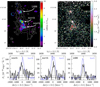 |
Fig. 10. Detection of extended He IIλ1640 fuzz in three distinct regions within LAB 1. Top left: map of the maximal He II S/N after cross-correlation with a 3D Gaussian template (see Sect. 5.2). We show the maximum from the S/N datacube between λmin = 6719 Å and λmax = 6729 Å (i.e. ±5 Å around He II at z = 3.1). We label the three He II emitting regions “south”, “north”, and “LAB8” as indicated. Top right: adaptive He II narrow-band image. The creation of this image followed a similar procedure as for the adaptive Lyα narrow-band image (see Fig. 5 and Sect. 5.2), except that here, the adopted S/N analysis threshold is three, and the default band-width for non-detections above this threshold is set to three datacube layers. The adaptive narrow-band image was additionally smoothed with a σ = 1 px (0.2″) Gaussian kernel. Grey contours indicate Lyα surface-brightness levels SBLyα = [200, 100, 50, 25, 8.75] × 10−19 erg s−1 cm−2 arcsec−2 as measured in the adaptive narrow-band image (Fig. 5). In addition to the foreground galaxies in the west, where bright continuum-emission corroborated the median-filter subtraction continuum removal, we also masked out O III line emission from a z = 0.3 galaxy (at the northern edge of the image), and Hβ emission from a z = 0.4 galaxy (at the north-western edge of the image), as these highly significant emission lines coincide with the z = 3.1 He II emission. Bottom panels: He II spectral profiles extracted from the three regions “south” (bottom left panel), “north” (bottom centre panel), and “LAB 8” (bottom right panel). The black line is the spectrum and the grey line shows the propagated error from the variance cube. The bottom axis is given in velocities and the top axis indicates rest-frame wavelength, both for z = 3.1. The vertical dotted line indicates the rest-frame wavelength of He II (1640.42 Å). Extraction was performed by defining apertures connected regions of pixels above a S/N threshold of 6 in the maximum S/N map. For comparison we also show the Lyα profiles scaled by a factor of 10 (5) for the “south” (“north” and “LAB8”) regions as blue lines (for those profiles, only the bottom velocity axis is relevant). |
We label the three regions where He II is detected with S/N > 6 “south”, “north”, and “LAB8” in Fig. 10. The “south” region is located south-west in proximity the ALMA continuum sources LAB1-ALMA1 and LAB1-ALMA2 while being slightly north-east of the Lyman-break galaxy SSA22a-C11. The “north” He II region cannot be associated with any known source in LAB 1. This region is co-spatial with the feature labelled “northern high SB region” in Fig. 4. It is also co-spatial with the region labelled R2 in Weijmans et al. (2010) and McLinden et al. (2013). Lastly, the “LAB8” region appears in proximity to the Lyman-break galaxy SSA22a-C15. We report the positions of those regions in Table 4. These positions are S/N-weighted, that is, calculated according to Eq. (1), with Ixy replaced by the pixel values of the maximum S/N map SNxy and only considering pixels satisfying SNxy ≥ 6 for each region. All He II peaks are within regions of Lyα surface-brightness above 5 × 10⁻¹⁸ erg s−1 cm−2 arcsec−2. However, the morphological features seen in He II are considerably different compared to the morphology of Lyα above this surface brightness limit.
Properties of He IIλ1640 emitting regions within the Lyα blob.
In order to extract 1D spectra from those regions, we created apertures consisting of contiguous regions with S/N > 5.5 in the maximum S/N image. The corresponding areas of these He II morphology-matched apertures are also listed in Table 4. The spectral profiles of the He II emission extracted in those regions are shown in the bottom panels of Fig. 10. Furthermore, we compare in this figure the He II spectral profiles to the Lyα profiles extracted in the same regions.
We measured the He II fluxes in those regions by summing the spectral profiles shown in Fig. 10 over their full width at zero intensity. The error on the fluxes was obtained from 104 Monte-Carlo (MC) realisations of the profile, where we used the propagated variances as input for adding noise to each spectral bin. The flux measurements obtained in this way are listed in Table 4. Given the areas of the extraction apertures, the measured fluxes correspond to He II surface-brightness values of 7.6 × 10⁻¹⁹ erg s−1 cm−2 arcsec−2, 5.7 × 10⁻¹⁹ erg s−1 cm−2 arcsec−2, and 7.6 × 10⁻¹⁹ erg s−1 cm−2 arcsec−2 for regions “south”, “north”, and “LAB8”, respectively. The measured He II surface brightness is ∼4−5 times fainter than the upper limits reported for a previous attempt to detect He II emission in LAB 1 using narrow-band imaging (Arrigoni Battaia et al. 2015).
To quantify the He II/Lyα flux ratios we measured the Lyα fluxes over their full width at zero intensity within the three He II emitting regions. We obtained FLyα = 1.7 × 10⁻¹⁶ erg s−1 cm−2, 1 × 10⁻¹⁶ erg s−1 cm−2, and 6.1 × 10⁻¹⁷ erg s−1 cm−2, corresponding to He II/Lyα 0.06 ± 0.01, 0.07 ± 0.01, and 0.10 ± 0.02, for regions “south”, “north”, and “LAB8”, respectively (see also Table 4). The errors on those ratios have also been computed from 104 MC simulations for the individual He II and Lyα flux measurements. From the previous non-detection of He IIArrigoni Battaia et al. (2015), which determined upper limits of He II/Lyα < 0.11 for LAB 1 and He II/Lyα < 0.22 for LAB8, the measured He II/Lyα ratios are a factor of two lower.
Using the first flux-weighted moment (Eq. (5)) on the extracted profiles, we determined the relative redshift offset between He II and the LyαΔv(zLyα) = c × (zLyα − zHeII)/(1 + zHeII). Again, the errors have been computed from 104 MC realisations.
A significant offset between Lyα and He II is only detected for the LAB 8 region, where Lyα appears modestly blue-shifted. Blue-shifted Lyα emission with respect to non-resonant nebular lines is atypical for normal Lyα emitting galaxies, that show often Δv(zLyα)≳200 km s−1 (e.g. Rakic et al. 2011; Song et al. 2014), although few exceptions exist (e.g. Trainor et al. 2015). Interestingly, our non-detections of velocity offsets between Lyα and He II around C11 and LAB 8 is consistent with the non-detection of offsets between Lyα and [O III] for those systems by McLinden et al. (2013). Moreover, Prescott et al. (2015b) also report similar low velocity offsets between He II and Lyα in a He II detected LAB at z = 1.67. These authors also compile data from the literature to show that LABs exhibit generally lower kinematic offsets between Lyα and optically thin lines and the measurements on He II emitting regions in LAB1 presented here corroborate this fact.
Lastly, it is visible in Fig. 10 that in all three regions, the Lyα profile appears broader compared to He II. To quantify this we measured the width of the He II and Lyα lines,  and
and  , using the second flux-weighted moment (Eq. (6), with k = 2). The measurements obtained are reported in Table 4. We find that Lyα is 1.6×, 2.4×, and 1.4× broader than He II in the “south”, “north” and “LAB8” region, respectively. These values are in agreement with the broadening of Lyα with respect to He II observed in a z = 1.67 LAB by Prescott et al. (2015b). As pointed out by these authors, the absence of significant velocity offsets between Lyα and He II and the presence of line broadening in Lyα with respect to He II are consistent with a scenario where a significant fraction of the extended Lyα emission is produced in situ. We discuss this physical interpretation further in Sect. 6.4.
5.6. Non-detection of the C IVλλ1548,1550 doublet
We detect no significant signal from the C IV doublet (1548.203 Å and 1550.777 Å) in the MUSE data of LAB 1. This can be seen in Fig. 11, where we show the maximum S/N map for C IV from evaluation of the 3D cross-correlated S/N datacube (see Sect. 5.2). Here the S/N cube was evaluated between λmin = 6345 Å and λmax = 6360 Å. While there are a few patches within the blob that indicate possible signal at S/N ≈ 5, this spectral region of the datacube is highly contaminated by sky-subtraction residuals. As these systematic residuals are not accounted for in the variance datacube, our S/N estimates are biased high. These sky-subtraction residuals appear especially pronounced at the edges of the individual observational datasets (see exposure map in Fig. 2). These edge-residuals are apparent as a patchy horizontal stripe of S/N ≈ 4 values slightly south of the photometric centre of LAB 8, as well as a vertical stripe on the western edge of the displayed region. A few pixels in the maximum S/N map show values above five in regions within the blob, but the extracted spectra in those regions do not show signal. We show in Fig. 11 the spectral region of interest around C IV for the spectra extracted within the three He II emitting regions (Sect. 5.5). In order to suppress the high-frequency sky-noise and residuals we also smoothed those spectra with a σ = 3.6 Å wide Gaussian. Interestingly, the smoothed spectrum – shown as a blue line in Fig. 11 – indeed appears to exhibit a small bump at the position of the λ1549 line in all three regions. However, from the noise in those three regions (shown as a grey line in Fig. 11), it is obvious that these features are not significant and can be only considered as a hint of C IV emission.
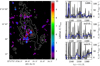 |
Fig. 11. Non-detection of significant signal from C IV emission within LAB 1. Left panel: maximum S/N after cross-correlation with a 3D Gaussian template (see Sect. 5.2). Here the S/N cube was evaluated between λmin = 6345 Å and λmax = 6360 Å. Right panels: spectral extractions in the regions “south”, “north”, and “LAB 8”, where significant He II emission was detected (Fig. 10). In each of those panels, the black curve shows the extracted spectrum, while the grey curve shows the propagated noise from the variance datacube. Vertical dotted lines indicate the rest-frame wavelengths of the C IV doublet. We also show a smoothed version (Gaussian window, σ = 3 px) of the spectrum (blue curve), which suppresses the high-frequency and high-amplitude oscillations from systematic sky-subtraction residuals in this wavelength range. |
To provide upper limits on C IV emission, we perform a source insertion and recovery experiment. For this experiment we assume that the C IV emission would be co-spatial with the He II emitting regions. As noted in Sect. 5.5, each of the three He II emitting region is defined by a cluster of connected spaxels that have S/N > 5.5. For simplicity, we assume constant surface brightness within each region. Furthermore, we model the spectral profile of the λλ1548, 1550 doublet by two Gaussians, where the dispersion is set to the average width measured from the He II line:  and we fix the ratio to 1.7 between λ1548 and λ1550. We implant the C IV emitting regions generated in this way at surface-brightness levels from 10−19 erg s−1 cm−2 arcsec−2 to 9 × 10⁻¹⁹ erg s−1 cm−2 arcsec−2 in steps of 10−19 erg s−1 cm−2 arcsec−2 prior to median-filter subtracting the fully reduced datacube. After median-filter subtracting each datacube with artificial C IV sources, we ran the 3D cross-correlation procedure from LSDCat. From this experiment, we found that we would detect the C IV emission significantly in all three regions at surface-brightness levels ≥8 × 10⁻¹⁹ erg s−1 cm−2 arcsec−2. Given the areas of the three He II emitting regions, our surface-brightness limit corresponds upper limits in C IV flux of 1.1 × 10⁻¹⁶ erg s−1 cm−2, 1.0 × 10⁻¹⁶ erg s−1 cm−2, and 6.1 × 10⁻¹⁶ erg s−1 cm−2 for regions “south”, “north”, and “LAB 8”, respectively. Given the measured Lyα fluxes in those regions (see Sect. 5.5), this corresponds to upper limits in C IV/Lyα ratios of 0.06, 0.1, and 0.11 for regions “south”, “north”, and “LAB 8”, respectively. Our upper limits on C IV translate into upper limits of < 1, < 1.4, < 1 of C IV/He II in regions “south”, “north”, and “LAB 8”, respectively.
Our upper limit for C IV emission within the He II emitting zones appears, at first sight, less constraining than the previous upper limit of 7.4 × 10⁻¹⁹ erg s−1 cm−2 arcsec−2 from narrow-band observations Arrigoni Battaia et al. (2015). However, the comparison has to be treated with caution, as the previous estimate assumed constant C IV emission over the whole area of the blob (∼200 arcsec2). Also, we assumed here that C IV emission is confined to the three He II emitting regions (≲10 arcsec2). The assumption of overlapping C IV and He II emission appears a good first-order approximation in scenario where C IV and He II act as a coolant of shock heated gas, as for both lines the maximum emissivity is obtained in a similar gas phase of T ∼ 105 K (Cabot et al. 2016), where C IV is driven through collisional excitations of C3+ (ionisation potential 47.9 eV), while He II is originating from the recombination cascade of collisionally ionised He2+ (ionisation potential 54.4 eV). Nevertheless, the C IV emissivity also peaks in a region of slightly lower density (nH ∼ 2−5 cm−3) compared to He II (nH ∼ 5−20 cm−3), thus C IV could potentially also be more extended (Cabot et al. 2016). This effect could be further enhanced by the resonant nature of C IV (see also Berg et al. 2019). On the other hand, if photo-ionisation from an AGN produces C4+ (ionisation potential 64.4 eV) that emits C IV as a result of recombinations, the C4+ zone would be confined within the He2+ zone. Lastly, we show below (Sect. 6.4) that under certain conditions, C IV might be even brighter than He II. For this reason, some detections of extended C IV without corresponding He II around quasars have been reported (Borisova et al. 2016; Travascio et al. 2020).
6. Discussion
6.1. Interpreting the moment maps of Lyα from LAB 1 as a tracer of gas kinematics
Before interpreting flux-weighted moment maps from Lyα as a tracer of gaseous motions, we need to asses how Lyα radiative transfer effects may have influenced these measurements. The Lyα velocity fields found to exhibit coherent large-scale kinematics have been observed around known (e.g. Arrigoni Battaia et al. 2018; Martin et al. 2019) or suspected (Prescott et al. 2015b) quasars. Details on the density distribution of the gas within those systems are still not settled, but it has been asserted that the strong ionisation field from the quasar produces a large fraction of Lyα photons in situ throughout the nebula via recombinations (e.g. Martin et al. 2014, 2019; Cantalupo et al. 2014, 2019). Nevertheless, even small residual neutral H I fractions (≲10−4) within the ionised halo result in high Lyα optical depths. Still, we suspect that the radiative transfer modulation of the Lyα profile for an extended intrinsic Lyα radiation field is less dramatic compared to the effect of an integrated spectrum within a compact Lyα emitting source. The reason is that the profile measured at each position in the nebula only reflects small local velocity offsets between point of emission and surface of last scattering (Prescott et al. 2015b). At typical spectral resolving powers, then, only a broadening of the Lyα line may be observed. This expectation appears consistent with our results for the He II emitting regions in LAB 1. Moreover, systemic literature redshifts of the galaxies associated with LAB 1 do not show significant offsets with respect to those determined from Lyα (McLinden et al. 2013; Kubo et al. 2016; Umehata et al. 2017). From this, we conclude that the first-moment map traces the gas-kinematics close to the embedded sources. For those galaxy near zones, we then can assume that significant amounts of Lyα photons must be produced in situ.
For interpreting the entire first-moment map as a tracer of the underlying gas kinematics, especially in regions far from known galaxies in LAB 1, we cannot resort to the argument above. The detection of polarised Lyα emission, both in imaging polarimetry (Hayes et al. 2011) and spectro-polarimetry (Beck et al. 2016), shows that significant fractions of the observed Lyα photons must have scattered into the line of sight after being emitted from a central source. According to radiative transfer theory the observed polarisation signal in Lyα stems from scattered photons within the wing of the absorption profile (e.g. Dijkstra & Loeb 2008; Eide et al. 2018). Hence, while these photons preserve information regarding the kinematics of the surface of last scattering, they appear red- or blue-shifted (depending on the kinematics of the scattering medium) with respect to the overall kinematics of the gas. Therefore, in a scenario where only scattered Lyα photons are observed at large distance to the embedded sources, the measured first-moments would be biased towards higher or lower velocities compared to the true gas kinematics. This could potentially increase the observed amplitude of the observed velocity gradient.
However, the above scenario also requires that significant amounts of Lyα photons are released by the dust-rich ALMA 850 μm detected galaxies in LAB 1 (see also Geach et al. 2016). The possibility of this process is indicated by the detection of Lyα emission from nearby ultra-luminous infrared galaxies (Martin et al. 2015a). Feedback-driven outflows powered by star formation is believed to create the required Lyα escape channels. Evidence for the required feedback effects at the positions of the galaxies comes from our higher-moment analysis discussed below (Sect. 6.3), but also from the spectro-polarimetry measurements by Beck et al. (2016). These authors find that the polarisation signal is increased in the wings of the Lyα profile, especially near the embedded galaxies. According to recent Lyα radiative transfer models of Eide et al. (2018) this is an expected polarisation signature in the presence of outflowing gas. Moreover, the Lyα escape channels produced by gaseous outflows can potentially also act as escape channels for ionising photons from the embedded systems, thus a significant fraction of those photons might indeed be available to power the emission from the blob via recombination. Empirical evidence for such a process has also been observed in the nearby universe (Herenz et al. 2017a; Bik et al. 2018; Menacho et al. 2019). Thus, in addition to Lyα scattering far from the embedded galaxies, we also expect that in LAB 1, a significant fraction of Lyα radiation is produced in situ at larger distances from the known embedded sources. Hence, the observed emission from the galaxy far-zones is likely superposition of scattered and in-situ produced Lyα emission. This potentially mitigates biases in the first moment maps that would result from pure Lyα scattering.
In summary, we present qualitative arguments in favour of interpreting large-scale coherent features in the first-moment map from Lyα as tracers of the gaseous motion in the system. These qualitative arguments have not yet been tested for Lyα radiative transfer simulations in realistic Lyα blob environments. As we also further discuss below, radiative transfer effects are, however, expected to strongly influence the Lyα line-width and the derived moments of a higher order. We suggest that the non-parametric moment-based measurements of the line profiles presented here also offer a starting point with which the complexity of the encountered profiles in LAB environments can be summarised. When guided by radiative transfer simulations, these measurements may help to disentangle scattering processes from in-situ Lyα photon production.
6.2. Combined analysis of Lyα line profile morphology and imaging polarimetry
Hayes et al. (2011) studied LAB1 using the FORS2 polarimeter at VLT in order to spatially map the polarimetric properties of the Lyα emission, including the Stokes vectors (Q and U), the polarised light fraction (P), and the angle of the linear polarisation vector (χ). The resulting maps of P and χ were qualitatively consistent with theoretical predictions by Lee & Ahn (1998), Rybicki & Loeb (1999), and Dijkstra & Loeb (2008), and implied a geometry in which Lyα is produced inside, or close to the central regions of the highest Lyα surface brightness (at the positions of the later-discovered ALMA sources 1 and 2) and scattered at large impact parameters, from vectors in the plane of the sky to the sightline of the observer. However the narrowband imaging polarimetry data contained no information regarding the kinematic properties of the Lyα emission, and we could not study where in the Lyα line profile the polarisation signal was imparted. To remedy this, Beck et al. (2016) conducted spectroscopic polarisation observations with the same instrument to study P and χ as a function of frequency. Those observations showed that the wavelength dependence of P is small near line centre, but rises towards the line wings. This is, again, qualitatively consistent with the numerical predictions of Dijkstra & Loeb (2008). Those slit data contained the necessary frequency information, but only at eight positions identified along the 1″ wide slit. Moreover, those studies were limited to the regions of highest surface brightness (Beck et al. 2016, their Fig. 3).
In this section, we use the 3D spectroscopy provided by MUSE to shed further light on the origin of the polarisation pattern. We perform a hybrid study and contrast the spatially derived (but spectrally unknown) measurements of P and χ with the Lyα kinematics using 3D spectroscopy. Hayes et al. (2011) used Voronoi tessellation to locally enhance the S/N in the images taken in individual beams (“ordinary & extraordinary”) and we apply the same binning patterns to the MUSE data: we aligned the FORS2 Lyα intensity images with the MUSE data, and propagate the recovered astrometric information into the maps of P and χ. For every Voronoi tessellated cell, we then extract the corresponding spaxels from the MUSE datacube and compute the moments described in Sect. 5.3.
Figure 12 shows the results, where we display the absolute velocity offset from zLyα = 3.1 (left panel) and the velocity dispersion (right panel). We show the absolute value of the first moment because the polarisation signal is imparted by wing scatterings, and scatterings in both the blue and red wings manifest in the same P (the quantity measured in our polarimetry data Dijkstra & Loeb 2008). We find a positive correlation between P and the absolute line-of-sight velocity, and also an anti-correlation between P and the velocity dispersion. The p-values of 10−5 − 10−4 suggest that correlations of this magnitude or larger are very unlikely to have arisen by a random process. The fact that Lyα should exhibit higher degrees of polarisation for narrow lines is a curious result and may stem from several effects.
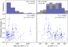 |
Fig. 12. Region-by-region comparison of the polarisation fraction (P) derived from VLT/FORS2 observations, with the kinematic measurements of the Lyα emission derived in this paper. Left panel: P against the absolute value of the first moment (Eq. (7)), right panel: P against the second moment (Eq. (8)). Gray points show every spatial element for which P could be measured at better than 5 per cent (see Fig. 2 of Hayes et al. 2011). Blue points show the regions in which P is detected at significance better than 2-σ. Spearman’s rank correlation coefficient, ℛ, and the associated p-value (the likelihood with which a correlation of at least this magnitude arises purely by chance) are shown in each figure – p < 0.05 is generally considered significant. The histograms above each plot shows the distribution of properties from the lower abscissae, where the grey and blue colouring follows that of the lower figures. The values from the two-sample KS-statistic, and the associated p-value, are presented in each panel. These p-values of almost 1 show that the polarised spaxels are consistent with being drawn from the same distribution, and that the trends seen in the blue points of the lower figures are not the result of biased selection. |
The polarisation data show a high P and a pattern in χ that is nearly tangentially aligned with a central source and that follows contours of surface brightness at smaller scales (Hayes et al. 2011, Fig. 2). To impart such a pattern, scattering in the wing of the redistribution profile needs to be promoted, so as, in turn, enhance scattering through the 2P3/2 excited level (Dijkstra & Loeb 2008; Eide et al. 2018). The P instead decreases if too many core (resonance) scattering events occur (through the 2P1/2 level). Such an enhancement of wing events cannot be the case for a static medium, where the gas would absorb Lyα close to line-centre (core). Some velocity offset is needed, which implies that high P should avoid |Δvlos|=0 (the original motivation for the outflowing shell models of Dijkstra & Loeb 2008). Moreover, even if large bulk velocity offsets are present, the velocity dispersion cannot be significantly larger than the absolute |vlos|: the consequence of a broad velocity range of absorbing material always leaves some high column density gas close to line-centre, and maintain significant core scattering. In a complex, 3D environment with multiple sources of Lyα and many velocity components of scattering gas, highly polarised regions should favour larger velocity shifts and narrower lines, and we would expect P to correlate with |vlos| and anti-correlate with the line width. This is precisely what Fig. 12 shows. In addition, the combination of 2D polarimetric data and 3D spectroscopic data supports a scenario in which preferential scattering outside the Doppler core is enhanced by velocity differences.
6.3. Insights into LAB 1 from the spatially resolved line-profile analysis
6.3.1. Large-scale gas kinematics from the first-moment map
We conclude in Sect. 6.1 with an assessment that the first-moment map from Lyα (Fig. 7, left panel) can be used to trace the large-scale kinematics of the gas within the blob. As seen from that map, the blob shows a coherent large-scale velocity gradient from receding velocities on its eastern side to approaching velocities on its western side. This large-scale velocity gradient encompasses LAB 1 and the northern neighbour LAB 8. Moreover, the newly detected shell-like region in the south-west (SW) of the blob is completely blue-shifted, seemingly following the large-scale E–W velocity gradient. Furthermore, also within the shell, a gradient from NW to SE is seen. The velocity field is mostly coherent over ∼150 kpc and shows significant perturbations only on smaller (≲30 kpc) scales.
We quantify the amplitude of the large-scale velocity shear as vshear = (vmax − vmin)/2 = 1304 km s−1, where vmax and vmin are the lower and upper 5th percentile of the observed first moments throughout the blob (this choice of percentiles is robust against outliers while sampling the true extremes of the distribution). Coherent large-scale velocity fields of such a large amplitude appear to be rare among extended Lyα nebulae around quasars at redshifts similar to LAB 1 (Borisova et al. 2016; Arrigoni Battaia et al. 2019). Nevertheless, a few comparable examples do exist: object 3 (Q0042-2627) in Borisova et al. (2016) and the QSO UM 287 studied in Martin et al. (2015b, 2019), as well as object 13 from Arrigoni Battaia et al. (2019) that was described in detail in Arrigoni Battaia et al. (2018). Moreover, two of the four QSOs in the recent z ∼ 6 sample by Drake et al. (2019) show coherent kinematics, while the other two objects show highly irregular and disturbed velocity fields.
We hypothesise that the preponderance of disturbed velocity fields around QSOs could be related to large-scale AGN-feedback effects. As an additional hypothesis, we state that the large fraction of chaotic velocity fields around QSOs is driven by the short exposure times that are typically used in those studies (e.g. 1 h in Borisova et al. 2016; 45 min in Arrigoni Battaia et al. 2019). These short exposures result in lower S/N for low-SB Lyα emission in the outskirts of the halos and potentially even miss the faintest regions, where large-scale kinematics may become most apparent. Comparing our observations with previous IFS observations of LAB 1 by Bower et al. (2004) and Weijmans et al. (2010), which additionally have a coarser spatial resolution (0.4″ per spaxel, and seeing FWHM≈1.5″) compared with our data (0.2″ per spaxel, and seeing FWHM≈0.9″), we indeed find that their velocity fields represent just a coarser and more noisy representation of the here observed velocity field in the high SB regions of the blob. Nevertheless, Bower et al. (2004) described the overall velocity structure of LAB 1 as chaotic with a lack of velocity shear. And undeniably, the velocity field of LAB 1 within the high-SB regions (SBLyα ≳ 10−18 erg s−1 cm−2 arcsec−2) appears complicated. As noted by Weijmans et al. (2010) the observed complexity in this region can be broken down into several sub-regions that show coherent velocity shear and some of these regions are associated to known galaxies within the LAB. These small-scale perturbations, now observed at higher spatial resolution in the MUSE data, might be related coherent motions of the gas in the individual sub-halos. But they also could be caused by kinematic perturbations due to inflowing cold gas, or they could be driven by feedback effects (see Sect. 6.3.2 below).
The most striking feature of the newly revealed large-scale velocity field is that the shear is observed perpendicular to the morphological principal axis (Fig. 7, left panel). The existence of such a large-scale coherent velocity field of high-amplitude appears in qualitative agreement with the theoretical predictions of hydro-dynamical simulations in a ΛCDM framework. In particular, it is a natural outcome of the filamentary nature of the cosmic web and the predicted existence of dense cold-gas streams that can penetrate deeply into dark-matter potential wells without being shock-heated by the gravitational potential (see review by Stewart et al. 2017). However, the perpendicular alignment between the velocity field and the morphological principal axis implies that the angular momentum vector of the gas in LAB 1 is aligned in parallel to the morphological principal axis. Simulations in the ΛCDM framework predict that the angular momentum vector and the elongation of the dark matter halos – including their gaseous and stellar contents – show correlated properties with the surrounding large-scale structure of the cosmic-web (e.g. Forero-Romero et al. 2014; Libeskind et al. 2018; Codis et al. 2018; Wang & Kang 2018, and references therein). These studies predict that the angular-momentum of high-mass halos (≳1012M⊙) is expected, on average, to be orthogonal with respect to the major axis of the halo, and the halo’s major axis is expected to be aligned in parallel to the connecting filament of the cosmic web. Thus, the observed alignment between morphological principal axis, which we naively interpret as the direction of the major cosmic web filament (as suggested by Erb et al. 2011), renders LAB 1 as an outlier from the theoretically expected average for high-mass halos.
We speculate that the deviation from the theoretically expected norm in LAB 1 is caused by the complexity of the surrounding large-scale structure. We regard the observed multi-filamentary morphology of the blob, with one filament extending to the SE in the direction of the two newly identified LAEs (labelled “filament towards LAE 3” in Fig. 4), another filament extending to the north (“filament to LAE 4” in Fig. 4), and another filament connecting to the shell-like region in SW (“shell-connecting filament” in Fig. 4) as evidence for such a complex environment. In fact, the SSA 22 proto-cluster, which hosts LAB 1 and LAB 8, is one of the most-massive structure known in the high-redshift universe (see Kikuta et al. 2019 for another extreme overdensity at z = 2.84). In such a high-z high-density peak of the universe a complex interwoven network of filaments is expected. Indeed, recent MUSE observations (texp ≈ 4 h) by Umehata et al. (2019) have revealed such a cold-gas network in Lyα at the core of SSA 22, located 4.8 ′ (2.19 Mpc) north-east of LAB 1. Interestingly, also this structure shows a mix of perpendicular and parallel-aligned large-scale velocity gradients with respect to the filamentary structure (Umehata et al. 2019, their Fig. 3).
The complexity of angular momentum alignments in dense cosmic regions was studied in simulations by Lee et al. (2018), who also showed that in these environments, the orientation of angular momentum vector is expected to change frequently and significantly. In such a scenario, the observed alignment of LAB 1’s angular momentum can be reconciled as an early evolutionary stage of a massive galaxy.
6.3.2. Small-scale kinematical perturbations in the first-moment map
As mentioned earlier in this paper, the coherent velocity field of LAB 1 shows also various perturbations on smaller scales. One prominent perturbation occurs at the position of the Lyman-break galaxy SSA22a-C11, where the velocity shears from north-west to south-east, that is, almost perpendicular to the apparent large-scale motion. The coherent small-scale velocity shear at the position of SSA22a-C11 was already noted by Weijmans et al. (2010). In this region, the velocity field varies from ∼450 km s−1 to ∼ −1500 km s−1 just within 2″ or 15 kpc in projection. It appears as if Lyα traces the velocity field of this individual bright galaxy that is not aligned with the blob’s large-scale velocity field. Such misalignments of sub-halos are also in qualitative agreement with the theoretical studies mentioned in the previous section (e.g. Codis et al. 2018). However, especially given the large amplitude on small physical scale, this disturbance of the velocity field may also be caused by feedback effects (galactic outflows, as proposed by Weijmans et al. 2010). Less prominent disturbances are apparent near the sub-mm detected sources LAB1-ALMA1 and LAB1-ALMA2. Here, as we discuss below in Sect. 6.3.3, the analysis of the moment maps of higher orders provides arguments in favour star formation-driven winds or outflows.
While the small-scale perturbations may be caused by individual velocity fields of the embedded galaxies or star-formation driven winds or outflows, we also have to consider the alternative (but not competing) hypothesis that they may in fact represent evidence for cold-flow multi-filamentary inflows. Recently, Martin et al. (2019) presented a quantitative framework to fit the expected kinematic signatures from cold-flow accretion streams to Lyα intensity-weighted velocity maps. These authors motivate their parametric ansatz by numerical simulations of a galaxy that exhibits cold filamentary inflows. The velocity field of this simulation was found to be optimally described by a large-scale rotating component that is modulated by radially and azimuthally varying components. These modulations are shown to capture the kinematic perturbations caused by the filamentary cooling flows. Martin et al. (2019) show that these parametric models also provide an excellent fit to the observed Lyα velocity fields of two large extended Lyα nebulae around radio-quiet quasars. We find that the qualitative appearance of velocity field modulations caused by the cooling flows in the Martin et al. (2019) ansatz bear similarity to the small-scale perturbations seen in LAB 1’s first-moment map. A quantitative treatment with the Martin et al. (2019) ansatz is, however, beyond the scope of the present analysis.
6.3.3. Interpretation of higher-order moment maps
Empirical insights into the Lyα photon production and/or scattering mechanisms within the blob can be gained from our maps of the Lyα line-width (Fig. 7, right panel), its skewness, its kurtosis κ, as well as its bi-modality (Fig. 8). In the following, we discuss several notable features in those maps. By visually inspecting the spaxels in each of the discussed regions, we ensure that the mapped values are indeed representative of the observed line profile morphology.
The highest line-widths (σv ≳ 500 km s−1) are observed N and S of LAB1-ALMA1 and LAB1-ALMA2. Towards the north this high dispersion regions shows a V-shaped morphology that traces the edges of the prominent “bubble” feature seen in the narrow-band image (Fig. 5). While Lyα shows no pronounced double peaked profile (b ≳ 2.6) at the position of LAB1-ALMA1 and LAB1-ALMA2, more pronounced double peaks are observed in the V-shaped region (b ∼ 2), with the NE arm showing the most pronounced double peaks (b ≲ 1.8). Thus, while it is tempting to interpret the broad widths close to the sub-mm source as gas that is kinematically hotter due to feedback from the galaxies, the measured large width of the profiles in those regions is rather the result of double component Lyα profiles, that is, Lyα radiative transfer.
However, we might witness possible signatures of outflowing gas traced by the Lyα skewness at the position of LAB1-ALMA1, where the Lyα profiles show a pronounced skew towards the blue (s ≲ −0.3). Interestingly, the Lyα profiles in some of the Martin et al. (2015a) ULIRGs show profiles with a blue tail. Martin et al. (2015a) interpret these blue tails as outflow signatures, with the Lyα in the wing being produced by gas cooling within the outflow. Also, south-east of LAB1-ALMA3 strong blue-skewed profiles that are indicative of an outflow are observed. This is corroborating the inference by Umehata et al. (2017), who argued that the properties of the [C II] 158 μm emission from LAB1-ALMA3 are suggestive of an interaction between a galactic outflow with an intergalactic gas stream.
As can be seen from Fig. 7, the line-width of Lyα is narrower in the outskirts of the blob. Both the shell-like region in the south-west and the filament emanating to the N and connecting to LAB 8, as well as the filament emanating to the north-east are characterised by σv ≲ 200 km s−1. However, as traced by the higher-moment based statistics (Fig. 8), even in those regions the observed Lyα line profiles appear to be quite complex. For example, along the LAB 1 - LAB 8 connecting filament the line profile is strongly skewed to the red (s ≳ +0.5). Most prominently this structure emerges as a red band in the skewness map. Throughout most of this filament, the discriminatory power of the adopted bi-modality indicator is weak (2.5 ≳ b ≳ 3). However, a visual inspection of the line profile hints, at least in some places, at the appearance of a secondary weaker red peak as cause for the measured red skew. For the north-east filament, observationally, the situation is more clear; here, the profile is clearly double peaked (b ≲ 2.5, see also example spectrum in panel 1 of Fig. 6), mostly with a weaker blue component. Both the red-skewed profiles with a potential secondary peak and the double peaked profiles are likely caused by radiative transfer. As discussed above (Sect. 6.2), the strongest polarisation signal arises in regions of smaller line-width (σv ≲ 250 km s−1), which is also supportive of Lyα scattering from a central source. Hence, the low-line width regions in the outskirts and in the filamentary regions hint at dense patches of gas where Lyα scattering takes place. The filamentary morphology of some of these patches is morphological reminiscent of cooling-flows, but whether the dominant Lyα signal is produced by cooling or photo-ionisation in those regions remains unclear. At least the line profiles in those regions appear consistent with a super-position of in-situ produced Lyα photons (dominant peak) and scattered Lyα radiation (wing or second component).
Another peculiar and outstanding feature in our higher moment-based maps is found at the northern edge of the bubble. Here the profile is significantly skewed (s ≳ +0.5) and described by a single-component (b ≳ 3) profile with a pronounced wing (κ ≈ 3.8). An aperture extracted Lyα spectral profile from this region is shown in panel 11 of Fig. 6. The bubble or cavity was already marked as a peculiar feature in LAB 1 by Bower et al. (2004). As a possible scenario Bower et al. (2004) discuss, that the bubble is filled by hot ionised gas. Bower et al. (2004) speculate that a potential radio-jet from the central sub-mm sources could have heated this gas. In this scenario, the skewed Lyα line arises in the region where the beamed emission is being slowed down by the denser cold-gas. Observational evidence for radio-emitting gas influencing the Lyα spectral properties have been presented for radio loud quasars and radio galaxies (e.g. Maxfield et al. 2002; Humphrey et al. 2007; Roche et al. 2014; Morais et al. 2017). However, no extended powerful radio-lobes are seen in the VLA 10 cm radio-continuum images and with S10 cm ≈ 7 μJy the nearby compact radio-continuum source is ∼103× weaker compared to typical radio-loud quasars (Ao et al. 2017). Moreover, Ao et al. (2017) remark a slight radio-excess compared to the expectation from the sub-mm determined star-formation, but they conclude that star-formation is a significant contributor in the heating of the gas. These observations appear compatible with the alternative hypotheses from Bower et al. (2004), which suggests that the cavity has been blown by a star formation-driven wind. The emergence of He II emission in the vicinity of the bubble may be linked to shock heated gas within the compressed shell of the bubble, although photo-ionisation by a potentially obscured radio-quiet AGN cannot be ruled out (see Sect. 6.4 below). Nevertheless, the Lyα profile in this region also shows a bump on the blue side and such a profile appears consistent with theoretically expected Lyα radiative transfer modulations within shock fronts (Chung et al. 2016).
Lastly, we note that at the position of C11 the Lyα profile is single-peaked (b > 3), but shows significant tails towards both the blue and red (κ > 3). Inspecting the profile from C11 we find that these wings appear to have substructure in the form of two additional peaks (see also panel 6 in Fig. 6). This triple-peaked structure is reminiscent of the Lyα profile from a multiply lensed-galaxy by Rivera-Thorsen et al. (2017), although not as extreme. Rivera-Thorsen et al. (2017) showed, that triple peaked Lyα profiles are indicative of low-covering fractions of neutral gas along the sight-line (see also Behrens et al. 2014). Thus, such galaxies potentially leak ionising radiation along the sight-line. Indeed, recently Rivera-Thorsen et al. (2019) confirmed the ionising photon leakage from their system. Thus, although C11 is located in an extremely dense environment, at least in its vicinity most of the gas appears highly ionised, thereby possibly promoting the escape of ionising radiation.
6.4. He II emission from the LAB: Driven by feedback, cooling flows, or hard ionising radiation?
In Sect. 5.5, we reported on the detection of three distinct extended He II emitting zones with SBHeII ∼ 6−7 × 10⁻¹⁹ erg s−1 cm−2 arcsec−2. Extended He II emission is commonly observed within the extended Lyα emitting regions surrounding high-z radio galaxies (e.g. Maxfield et al. 2002; Villar-Martín et al. 2007a,b; Morais et al. 2017; Marques-Chaves et al. 2019). Broad line profiles and alignments with the radio-jet axes indicate that He II is, at least in part, powered by jet-gas interactions in those objects. Detections of He II emitting zones within the extended Lyα nebulae surrounding radio quiet quasars or in LABs not directly associated with an AGN appear less frequent and more difficult to interpret (Scarlata et al. 2009b; Prescott et al. 2009; Cai et al. 2017; Cantalupo et al. 2019; Humphrey et al. 2019). Different explanations have been put forward, for example, Scarlata et al. (2009b) favouring cooling-radiation in their system or Prescott et al. (2009) arguing for photo-ionisation by an AGN or an extremely metal poor stellar population in their object, while Cai et al. (2017) reason that their extended He II zone is powered by shocks. We now try to constrain the physical mechanisms responsible for the extended He II emission in the blob. To this aim, we also consider the upper limits on C IV emission from the He II emitting zones in Sect. 5.6.
To place our result in context with previous observations (or upper limits) of He II and C IV emission from high-z sources with extended Lyα emission, we compare in Fig. 13 our measured He II/Lyα ratios and our derived upper limits on C IV/Lyα to the literature. The majority of comparison objects in Fig. 13 harbour a bright active galactic nucleus. We observe that that the ratios and upper limits in LAB 1 appear not unusual with respect to other extended Lyα objects, that is, some objects exhibit significantly higher ratios both in He II/Lyα and C IV/Lyα, but also significantly lower ratios or upper-limits have been reported. The diversity in ratios observed for nebulae with known powering source imply that varying physical conditions (e.g. metallicity, temperature, and density) within the emitting gas significantly influences the observed ratios. Additionally, radiative transfer effects in both Lyα and C IV (Berg et al. 2019, their Sect. 2.3) can also bias conclusions drawn from this diagram (e.g. Caminha et al. 2016). This diagram has now been frequently used in the literature for attempting to understand the physical conditions of the ionised gas.
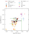 |
Fig. 13. Measured He II/Lyα ratios vs. upper limits on C IV/Lyα ratios for the three regions where we detect He II emission in the LAB (individually labelled black circles and error bars) in comparison to ratios or upper limits seen in other high-z sources with extended Lyα nebulae. The comparison includes the following objects from the literature: 61 high-z radio galaxies (labelled RG in the legend, with different symbols for the z < 3 and z ≥ 3 sources) from the compilation by Villar-Martín et al. (2007a); 17 radio-quiet quasars and two radio-loud z ∼ 3 quasars (labelled B16 – mostly upper limits in He II and C IV with only four sources with C IV detections, and with the two highest C IV/Lyα ratios coming from the radio-loud quasars) by Borisova et al. (2016); five extended 2 ≲ z ≲ 3 Lyα nebulae found in a blind broad-band search (labelled P13) from Prescott et al. (2013); the extreme Lyα nebulae around a z = 2.3 quasar MAMMOTH-1 from Cai et al. (2017); a z = 2.3 LAB from Scarlata et al. (2009a) that is detected only in He II (labelled S09); a faint (≈1042 erg s−1) extended nebulae found behind a gravitational lens (labelled C16) by Caminha et al. (2016); and an extended line emitting nebulae around a z = 2.5 radio-loud quasar (labelled H13) from Humphrey et al. (2013). We also show a track of a photo-ionisation model with varying ionisation parameter by Villar-Martín et al. (2007a) for a power-law spectral energy distribution with nH = 100 cm−3 and solar metallicity (labelled VM07 pi model – see text for details). |
We show in Fig. 13 the track of a photo-ionisation model from Villar-Martín et al. (2007a) that appears to be in good agreement with the He II/Lyα ratios and C IV/Lyα ratios from our observations. This track was computed for gas of solar metallicity at a density of nH = 100 cm−3 as a function of a varying (dimensionless) ionisation parameter
 (13)
(13)
where  denotes the rate of hydrogen ionising photons produced by the source and r denotes the distance of the ionised gas cloud to the source. As the spectral energy distribution of the ionising source, Villar-Martín et al. (2007a) assumed an idealised quasar described by a Fν ∝ να power-law continuum with slope α = −1.5. Along the displayed track log U varies from −2.3 (start of the upper branch) to 0 (end of the lower branch); the inflection point in C IV/Lyα is at log U = −1 (the model is adopted from Fig. 1 of Villar-Martín et al. 2007a).
While the predicted line-ratios show some agreement with our observation, for the region labelled “north”, the assumptions in this model require extremely high photo-ionisation rates: the region “north” is ∼50 kpc in projection towards LAB-ALMA1, LAB-ALMA2, and VLA-LAB1a. Thus, according to Eq. (13), even the smallest log U = −2.3 in the Villar-Martín et al. (2007a) model corresponds  s−1 if we assume a galaxy at the position of LAB-ALMA1, LAB-ALMA2, or VLA-LAB1a as the ionising source. This value would be similar to the photo-ionisation rate inferred for the luminous quasar UM 287 that powers the “Slug” nebulae (Cantalupo et al. 2014) and two orders of magnitude higher than the
  s−1 that would be required to power the whole blob via photo-ionisation (under case-B assumptions). While the photo-ionisation model might be more fitting for the zones marked “south” and “LAB 8”, as they are in close vicinity to known galaxies, existing deep multi-wavelength data does not find strong evidence in favour of such a luminous AGN (Ao et al. 2017). Thus, we also explore different mechanism that have been put forward to explain He II in LABs.
The co-spatial occurrence of He II emitting gas with embedded galaxies in the blob is qualitatively consistent with hydrodynamic simulations from Cabot et al. (2016) that do not contain photo-ionisation by an AGN. The Cabot et al. (2016) models predict that the main source of He II emission in LABs should be shock-heated gas from supernovae driven winds. Included in the simulations are both Lyα radiative transfer and dust-extinction effects, as well as photo-ionisation from a star-forming population at star-formation rates compatible with typical LABs (logSFR[M⊙ yr−1]∼2). In Fig. 14, we compare our measured He II/Lyα ratios and C IV/Lyα upper limits with the results from the 48 simulated LABs by Cabot et al. (2016). As can be seen our measured He II/Lyα ratios are significantly above the ratios predicted by the models, while our upper limits on C IV/Lyα are compatible with the models. The discrepancy between models and data may indicate that, contrary to the assumption simulations, shock heating is not the dominant mechanism in producing the observed He II/Lyα ratios. Alternatively, the physical properties of the 46 simulated halos by Cabot et al. (2016) might be significantly different from that of the halo hosting LAB 1.
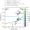 |
Fig. 14. Measured He II/Lyα ratios vs. upper limits on C IV/Lyα ratios for the three He II emitting regions in LAB 1 compared to hydrodynamic simulations from Cabot et al. (2016) and tracks of photo-ionisation models by Humphrey et al. (2019). The individual simulated LABs from Cabot et al. (2016) are colour-coded according to the star-formation rate of the galaxies within the LAB hosting halos. The Humphrey et al. (2019) photo-ionisation models are computed for low metallicity (Z = 0.01Z⊙) low-density gas in the circum-galactic medium of AGN host-galaxies (blue and green curve – see text) or Pop-III star-forming galaxies (orange curve). For the photo-ionisation models the ionisation parameter varies from U = 0.25 for the highest C IV/Lyα ratios to U ≈ −2.5 where C IV/Lyα = −3. |
We find a similar discrepancy between the He II/Lyα ratios in LAB 1 and recent AGN photo-ionisation models by Humphrey et al. (2019). As shown in Fig. 14, these models also predict significantly lower He II/Lyα than what is observed here. The Humphrey et al. (2019) photo-ionisation tracks were computed for different ionising sources illuminating low-metallicity (Z = 0.01Z⊙) gas. Similar to the calculations by Villar-Martín et al. (2007a) a gas density of nH = 100 cm−3 was adopted. The aim of these computations was to find an explanation of the extreme ratios or upper limits found for some nebulae around AGN or radio-galaxies that appeared incompatible with previous photo-ionisation attempts (see Fig. 13). We show in Fig. 14 the resulting predictions for photo-ionisation by an idealised quasar (described by a Fν ∝ να power-law continuum spectral energy distribution with α = −1.5, blue curve), whose ionising continuum also has been modified by intervening cold-gas that absorbs 50% of the ionising photons (green curve) and a fiducial zero-metallicity stellar population (modelled by a 8 × 10⁴ K black body) for varying ionisation parameters. In Fig. 14 the tracks are shown from U = 0.25 for the highest C IV/Lyα ratios to U ≈ −2.5 where C IV/Lyα = −3. Within the displayed range the He II/Lyα ratio exhibits a weak dependence on U, while the C IV/Lyα ratio rapidly decreases with decreasing U. The reason for the almost constant He II/Lyα ratio is that in the simulated low-metallicity gas the fraction of He++ ions remains saturated for an U ≳ −2.5 photo-ionisation field. On the other hand, the large decrease in C IV/Lyα for decreasing U is driven by both the reduction in electron temperature (resulting in lower collision rates for C3+) and the decreasing fraction of C3+ ions for smaller values of U. We remark also that for U < −2.5 (outside of the displayed range in Fig. 14, see Humphrey et al. 2019), the He II/Lyα ratios also start to decrease significantly. As explained above, for nH = 100 cm3 gas in region “north” only log U ≲ −4 would be compatible with a scenario where the whole blob is powered by photo-ionisation, but also at these extreme ionisation parameters the Humphrey et al. (2019) model are incompatible with our observations. Thus, photo-ionisation of low-metallicity gas by an AGN or Pop-III stellar population under the assumptions made in the Humphrey et al. (2019) models appears not to be a valid scenario to explain the He II emitting zones in LAB 1.
It is also apparent in Fig. 14 that the photo-ionisation tracks overlap with the predictions from the ab-initio simulations by Cabot et al. (2016) in which shock-heated emission dominates. A similar degeneracy was commented upon by Arrigoni Battaia et al. (2015), who computed a different set of AGN photo-ionisation models. Similar to Villar-Martín et al. (2007a), these authors modelled the expected line ratios in solar-metallicity optically-thick and optically-thin gas. Their optically-thin models are compatible with our He II/Lyα ratios at very low ionisation parameters (log U ≲ −2.5), where C IV/Lyα ≲ 10−2 (Fig. 12 in Arrigoni Battaia et al. 2015), that is, ≈10 times below our upper limit for this ratio. As discussed above, such low values of U are not unrealistic for the He II emitting zones within the LAB. On the other hand, their optically thick models (NH) would require relatively high ionisation parameters to reproduce our observed He II/Lyα ratios. For those models then, the predicted C IV/Lyα values would be slightly below our upper limits. Unfortunately, this region of the He II/Lyα vs. C IV/Lyα parameter space is also covered by shock models. This is illustrated by Fig. 15, where we compare our measurements and upper limits to the predictions from shock models at solar metallicity by Allen et al. (2008). For those models we use the same parameters motivated by Arrigoni Battaia et al. (2015) and we refer to Sect. 5.2 of their publication for an in-depth discussion of the motivation and description of the models.
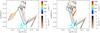 |
Fig. 15. Measured He II/Lyα ratios vs. upper limits on C IV/Lyα ratios for the three regions where we detect He II emission in the LAB compared to shock (left panel) and shock+precursor (right panel) models from Allen et al. (2008). We show all models for a constant magnetic parameter B/n1/2 = 3.23 μG cm−3/2. The grids are colour coded according to the density nH of the pre-shocked region and the shock velocity vs. We also show the predicted line-ratios from ab-initio hydro-dynamical simulations of z = 3 LABs by Cabot et al. (2016). |
As made evident by Fig. 15, both shock and shock+precursor models can reproduce the observed He II/Lyα ratios for C IV/Lyα ratios that would be consistent with our upper limits for shock velocities of vs ∼ 250−500 km s−1. While for the region marked “south”, the observed line-width in He II appears compatible with those velocities, the other two regions show significantly narrower He II emission. However, in particular, the emission stemming from the pre-cursor arises in kinematically more quiescent gas which is photo-ionised by the hard-UV radiation from the shock. The measured line-widths might thus indicate that we observe He II emission from the pre-shock phase.
A third interpretation for our He II detection is provided in the models from Yang et al. (2006). These models suggest that extended zones of narrow (≲250 km s−1) He II emission within Lyα blobs are a signature of gravitational cooling radiation. We here observe He II in close vicinity to star-forming galaxies (regions “south” and “LAB 8”) and next to the expanding bubble within the blob (region “north”). The Yang et al. (2006) models also predict the highest He II and Lyα surface brightness in close vicinity of the star-forming galaxies within the blobs. Considering only Lyα emission, a similar conclusion was recently reached by Trebitsch et al. (2016). Hence, our observations do not rule out contributions from cooling radiation within two of our three detected He II patches. But again, the region marked “north” is an exception as it not close to a known galaxy.
In summary, the detection of faint extended He II emission is consistent with all mechanisms that are suggested to power the Lyα blob – that is, cooling radiation, feedback driven shocks, or photo-ionisation from an embedded active galactic nuclei. For the latter two scenarios we compared He II/Lyα ratios and upper limits on C IV/Lyα with observed ratios from the literature and models. He II/Lyα and C IV/Lyα ratios comparable to our measurements have been found in extended Lyα halos around high-z radio galaxies and AGNs, and these ratios can be explained by some photo-ionisation models. However, our ratios are not as extreme as the ratios that would be expected from quasar photo-ionisation of extremely metal-deficient gas at very low ionisation parameters (Humphrey et al. 2019).
A potential caveat when comparing our measured line ratios with photo-ionisation models is that measurements were obtained within apertures that cover a projected area of ∼103 kpc2. We expect realistically that gas within those regions exhibits a range of different densities and temperatures. However, the observed He II/Lyα ratios from photo-ionised gas from an embedded quasar depend sensitively on the density distribution of the line emitting gas (Cantalupo et al. 2019). In fact, for any realistic density distribution the aperture integrated He II/Lyα ratio will always be lower than the intrinsic ratios within the volume covered by the aperture. Thus, the quantitative comparison between our measured line ratios and upper limits to photo-ionisation models must be treated with caution, as these models always assumed constant densities.
7. Summary and conclusions
In this work, we present an analysis of 17.2 h MUSE observations of the prototypical SSA22a LAB 1 at z = 3.1. Our analysis has revealed many previously unknown features of this enigmatic high-z object and provided detailed look into the early formation stage of a massive galaxy within an extremely dense environment. The main results of our study are the following:
-
Our IFS data reaches a limiting depth of ≈6 × 10⁻¹⁹ erg s−1 cm−2 arcsec−2 in Lyα. This is a factor of ten deeper than previous IFS observations of LAB 1 by Weijmans et al. (2010), which revealed Lyα down to 5.6 × 10⁻¹⁸ erg s−1 cm−2 arcsec−2. At this unprecedented depth, we uncovered several hitherto unknown features of the blob. Most prominently we find a filamentary bridge connecting LAB 1 with its northern neighbour LAB 8 and a shell-like arc towards the SW of LAB 1. Potentially another filament is emanating to the SE in the direction of two newly identified faint LAEs. These filamentary features are visible both in the sequence of 2.5 Å narrow-band slices (Fig. 3) as well as in the adaptive Lyα image (Fig. 5). The newly uncovered structures are morphologically reminiscent of cold streams that are predicted to funnel cool gas into the potential wells of massive halos. As cooling flows are expected to align with the underlying filamentary large-scale structure, the presence of multiple filaments pointing into various directions may imply that LAB 1 harbours a node in the cosmic web where a complex interwoven network of filaments arrives from various directions.
-
We find a ring-like structure slightly west of the photometric centre that is deprived of Lyα emission. While previous observations hinted already at the existence of this feature (Bower et al. 2004; Weijmans et al. 2010), the improved spatial resolution and sensitivity of our observations allow us to slice through this shell in velocity space (Fig. 3). The detection of He II emission at a He II/Lyα ratio, consistent with expectations for shock-heated gas in regions directly demarcating the “bubble”, appears supportive of the hypothesis that we are observing a genuine cavity filled by hot ionised gas. However, the line ratio is also consistent with photo-ionisation models that assume an AGN as ionising source, but the required photo-ionisation rates for those models appear too high when an AGN is assumed at the position of the central most plausible AGN sources (Sect. 6.4). Moreover, as seen in our higher-order moment maps (Fig. 8), the Lyα profile at this position is markedly different than in the surrounding regions – it is strongly skewed with a pronounced red tail, but not bi-modal. Such a profile is reminiscent of the Lyα radiative transfer simulations for expanding shells (Verhamme et al. 2006; Gronke & Dijkstra 2016); and, furthermore, the faint blue-wing seen in the profile (Fig. 6, panel 11) appears consistent with predictions for the Lyα profiles in shock-fronts (Chung et al. 2016). These results may indicate that pressure exerted by the hot ionised gas drives an expanding bubble (Sect. 6.3.3). Potential driving mechanisms for this expansion are a star formation-driven wind or radio emission from an obscured or faded AGN associated to the central sub-mm/radio sources.
-
The Lyα profiles observed from the blob exhibit varying degrees of complexity (Fig. 6). We tried to map the varying complexity of the blob by utilising a moment-based non-parametric analysis of the profiles (Sect. 5.3). This analysis provided us with maps of the line of sight velocity (central moment), the width of the line, its skewness, kurtosis, and bi-modality (Figs. 7 and 8). In particular, within the central regions of the blob, we find broad double- or even triple-peaked profiles. Unfortunately, however, for these complex broad profiles the used bi-modality measure from Remolina-Gutiérrez & Forero-Romero (2019) did not appear to be very precise. However, it spatially pinpoints three compact regions that are characterised single peaked profiles that are sometimes skewed towards the blue or the red. Two of these regions are associated with the known Lyman-break galaxies, SSA22a-C11 and SSA22a-C15, and the third is associated with the edge of the expanding bubble. Interestingly, these single peaked features appear in the vicinity of the He II emitting zones. The spatially varying complexity of the profiles likely encodes a mix of different Lyα photon production mechanisms: in-situ production from ionising sources and gravitational cooling, or both simultaneously. Moreover, projection effects from the line-of-sight passing through multiple filaments may also be responsible for the appearance of multiple peaks. Single peaked profiles might indicate a small residual fraction of neutral gas at line centre, and therefore pinpoint a high degree of ionisation. Quantitatively disentangling the production mechanisms and projection effects based on the line profiles appears notoriously difficult. An analysis of realistic Lyα blob simulations in a cosmological context, as presented very recently, for example, by Kimock et al. (2020), could reveal whether the moment presented here has diagnostic power in this respect.
-
We find the highest degrees of Lyα polarisation in regions that exhibit high velocity shifts and narrow line profiles (Sect. 6.2 and Fig. 12). These regions are far from known embedded galaxies. It appears that this result is consistent with theoretical expectations for Lyα scattering from a central source (Eide et al. 2018), although numerical simulations for Lyα spectro-polarimetry in complex 3D environments have yet to be performed.
-
The line-of-sight velocity field of the blob is characterised by a large-scale velocity gradient that is oriented perpendicular to the morphological major axis of the blob (Fig. 7, left panel). The observed shearing amplitude is vshear ≈ 1300 km s−1. The orientation of the velocity gradient implies a parallel alignment between angular momentum vector and major axis. This parallel alignment between major axis and angular momentum appears at odds with the theoretically expected average for massive halos (Sect. 6.3.1). We argue that this peculiar alignment reflects the complexity of the dense environment in which the blob resides. This leads us to speculate that LAB 1 is formed at the node of multiple intersecting filaments of the cosmic web. The kinematic interpretation of the large-scale velocity field relies on the assumption that the first-moment map from Lyα is a good tracer of the large-scale kinematics (Sect. 6.3.1), an assumption that has of yet not been tested against radiative-transfer simulations.
-
We detect extended He IIλ1640 emission at three disjunct regions in the blob (Sect. 5.5 and Fig. 10). The He II emission from those regions shows a surface brightness of 5−7 × 10⁻¹⁹ erg s−2 cm−2 arcsec−2. Two of those regions surround known embedded galaxies and the third region demarcates the expanding bubble. Our observations do not reveal C IVλ1549 emission from those regions (Sect. 5.6). A comparison between predicted He II/Lyα and C IV/Lyα ratios from shock- and photo-ionisation models from the literature with our measurements and upper limits is consistent with both photo-ionisation from an AGN (Villar-Martín et al. 2007a) and fast radiative shocks (Allen et al. 2008). However, the observed ratios were found to be incompatible with recent AGN photo-ionisation models by Humphrey et al. (2019) that assume low-gas metallicity, an ionising source partly covered by optically thick neutral gas, or very low ionisation parameters. Moreover, our observed He II/Lyα ratios are also significantly above the predicted ratios from the hydrodynamic simulations of Cabot et al. (2016) that predict feedback-driven shocks and gas accretion-shocks as main source for the observed He II emission in LABs.
Our new observations provide the most detailed view of a Lyα blob to date. Given the large number of galaxies within the blob and the surrounding dense proto-cluster environment, it seems natural to suspect LAB 1 may be the progenitor of a massive cluster elliptical. The detection of He II emission may hint at the importance of feedback effects in the early evolutionary stage of such systems, but AGN-powering cannot be ruled out. Moreover, we find no clear evidence for gravitational cooling, but, also, we cannot rule this mechanism out. We suggest that simulations of Lyα blobs in cosmological environments should be compared to the non-parametric line profile analysis presented here. Moreover, rest-frame optical emission line studies with, for example, the James Webb Space Telescope, will help to better constrain the powering mechanisms. Finally, our study also highlights the potential importance of environmental effects on the kinematic properties of massive halos that lie at the intersection of multiple filaments of the cosmic web. As our study focusses on a single object, we cannot establish any empirical trends in this respect, therefore, future studies of LAB samples at sufficient depths in proto-cluster environments would provide more valuable information.
We note the coordinates for these Lyman-break galaxies provided in Steidel et al. (2003) – RA = 22h17m25.67s/Dec = +00°12′35.2″ for SSA22a-C11, and RA = 22h17m26.127s/Dec = +00°12′55.3″ for SSA22a-C15 – appear to be offset by ∼1″ to the north-west with respect to where these galaxies are located in our data. As described in Sect. 4.2, we aligned our data with the 2MASS reference frame, while Steidel et al. (2003) tied their astrometry the HST guide star catalogue. Earlier versions of the HST guide star catalogue were known to contain systematic errors of up to ∼1″ (Morrison et al. 2001). We thus speculate that this is the reason for the coordinate offsets. Here we revise the coordinates of SSA22a-C11 and SSA22a-C15 according to our adopted reference frame (Table 1).
The to our science observations associated spectrophotometric standards are Feige110, GJ754.1A, GD153, EG274, LTT3218, GD108, and LTT7987.
LSDCat is publicly available via the Astrophysics Source Code Library: http://ascl.net/1612.002 (Herenz & Wistozki 2016).
We determined the PSF FWHM via fitting a 2D Gaussian profile to the bright star within our field of view in a 45 Å wide narrow-band image centred at zLyα = 3.1.
In general for compact point-sources the relation S/Nmax ∝ 2κ/(κ + 1)2, with FWHMfilt = κ × FWHMPSF holds, where FWHMfilt and FWHMPSF denote the adopted width of the filter and the width of the point-spread function, respectively (Herenz & Wisotzki 2017).
All SBLyα measurements were obtained within an circular aperture of 2″ diameter.
The QFitsView software is publicly available via the Astrophysics Source Code Library: http://ascl.net/1210.019.
We use the air-to-vacuum wavelength conversion that has been adopted in the Vienna Atomic Line Database (Ryabchikova et al. 2015): https://www.astro.uu.se/valdwiki/Air-to-vacuum%20conversion.
Acknowledgments
We thank the anonymous referee for a careful report that contained many suggestions that helped to improve this paper. E. C. H. thanks the extragalactic group at Stockholm University for a wonderful time and many insightful discussions during this project. E. C. H. also thanks Aaron Smith and Peter Laursen for useful comments during early stages of this project. This research made extensive use of the astropy package (Astropy Collaboration 2018). All figures in this paper were created using matplotlib (Hunter 2007).
References
- Alexander, D. M., Simpson, J. M., Harrison, C. M., et al. 2016, MNRAS, 461, 2944 [CrossRef] [Google Scholar]
- Allen, M. G., Groves, B. A., Dopita, M. A., Sutherland, R. S., & Kewley, L. J. 2008, ApJS, 178, 20 [Google Scholar]
- Ao, Y., Matsuda, Y., Beelen, A., et al. 2015, A&A, 581, A132 [NASA ADS] [CrossRef] [EDP Sciences] [Google Scholar]
- Ao, Y., Matsuda, Y., Henkel, C., et al. 2017, ApJ, 850, 178 [Google Scholar]
- Arrigoni Battaia, F., Yang, Y., Hennawi, J. F., et al. 2015, ApJ, 804, 26 [NASA ADS] [CrossRef] [Google Scholar]
- Arrigoni Battaia, F., Prochaska, J. X., Hennawi, J. F., et al. 2018, MNRAS, 473, 3907 [NASA ADS] [CrossRef] [Google Scholar]
- Arrigoni Battaia, F., Hennawi, J. F., Prochaska, J. X., et al. 2019, MNRAS, 482, 3162 [NASA ADS] [CrossRef] [Google Scholar]
- Astropy Collaboration (Price-Whelan, A. M., et al.) 2018, AJ, 156, 123 [Google Scholar]
- Bacon, R., & Monnet, G. J. 2017, Optical 3D-Spectroscopy for Astronomy (Wiley-VCH Verlag GmbH & Co. KGaA) [CrossRef] [Google Scholar]
- Bacon, R., Accardo, M., Adjali, L., et al. 2010, in Society of Photo-Optical Instrumentation Engineers (SPIE) Conference Series, SPIE Conf. Ser., 7735 [Google Scholar]
- Bacon, R., Vernet, J., Borisiva, E., et al. 2014, Messenger, 157, 13 [Google Scholar]
- Bacon, R., Piqueras, L., Conseil, S., Richard, J., & Shepherd, M. 2016, MPDAF: MUSE Python Data Analysis Framework (Astrophysics Source Code Library) [Google Scholar]
- Bacon, R., Conseil, S., Mary, D., et al. 2017, A&A, 608, A1 [NASA ADS] [CrossRef] [EDP Sciences] [Google Scholar]
- Bădescu, T., Yang, Y., Bertoldi, F., et al. 2017, ApJ, 845, 172 [CrossRef] [Google Scholar]
- Barger, A. J., Cowie, L. L., & Wold, I. G. B. 2012, ApJ, 749, 106 [CrossRef] [Google Scholar]
- Beck, M., Scarlata, C., Hayes, M., Dijkstra, M., & Jones, T. J. 2016, ApJ, 818, 138 [CrossRef] [Google Scholar]
- Behrens, C., Dijkstra, M., & Niemeyer, J. C. 2014, A&A, 563, A77 [NASA ADS] [CrossRef] [EDP Sciences] [Google Scholar]
- Berg, D. A., Chisholm, J., Erb, D. K., et al. 2019, ApJ, 878, L3 [NASA ADS] [CrossRef] [Google Scholar]
- Bik, A., Östlin, G., Menacho, V., et al. 2018, A&A, 619, A131 [NASA ADS] [CrossRef] [EDP Sciences] [Google Scholar]
- Borisova, E., Cantalupo, S., Lilly, S. J., et al. 2016, ApJ, 831, 39 [NASA ADS] [CrossRef] [Google Scholar]
- Bower, R. G., Morris, S. L., Bacon, R., et al. 2004, MNRAS, 351, 63 [NASA ADS] [CrossRef] [Google Scholar]
- Bridge, J. S., Hayes, M., Melinder, J., et al. 2018, ApJ, 852, 9 [NASA ADS] [CrossRef] [Google Scholar]
- Brooks, A. M., Governato, F., Quinn, T., Brook, C. B., & Wadsley, J. 2009, ApJ, 694, 396 [NASA ADS] [CrossRef] [Google Scholar]
- Cabot, S. H. C., Cen, R., & Zheng, Z. 2016, MNRAS, 462, 1076 [NASA ADS] [CrossRef] [Google Scholar]
- Cai, Z., Fan, X., Yang, Y., et al. 2017, ApJ, 837, 71 [NASA ADS] [CrossRef] [Google Scholar]
- Caminha, G. B., Karman, W., Rosati, P., et al. 2016, A&A, 595, A100 [NASA ADS] [CrossRef] [EDP Sciences] [Google Scholar]
- Cantalupo, S. 2017, in Gas Accretion onto Galaxies, eds. A. Fox, & R. Davé, Astrophys. Space Sci. Lib., 430, 195 [NASA ADS] [CrossRef] [Google Scholar]
- Cantalupo, S., Arrigoni-Battaia, F., Prochaska, J. X., Hennawi, J. F., & Madau, P. 2014, Nature, 506, 63 [NASA ADS] [CrossRef] [Google Scholar]
- Cantalupo, S., Pezzulli, G., Lilly, S. J., et al. 2019, MNRAS, 483, 5188 [NASA ADS] [CrossRef] [Google Scholar]
- Chapman, S. C., Lewis, G. F., Scott, D., et al. 2001, ApJ, 548, L17 [NASA ADS] [CrossRef] [Google Scholar]
- Chapman, S. C., Windhorst, R., Odewahn, S., Yan, H., & Conselice, C. 2003, ApJ, 599, 92 [NASA ADS] [CrossRef] [Google Scholar]
- Chapman, S. C., Scott, D., Windhorst, R. A., et al. 2004, ApJ, 606, 85 [NASA ADS] [CrossRef] [Google Scholar]
- Childs, H. J. T., & Stanway, E. R. 2018, MNRAS, 480, 1938 [CrossRef] [Google Scholar]
- Chonis, T. S., Blanc, G. A., Hill, G. J., et al. 2013, ApJ, 775, 99 [NASA ADS] [CrossRef] [Google Scholar]
- Christensen, L., Jahnke, K., Wisotzki, L., & Sánchez, S. F. 2006, A&A, 459, 717 [NASA ADS] [CrossRef] [EDP Sciences] [Google Scholar]
- Chung, A. S., Dijkstra, M., Ciardi, B., & Gronke, M. 2016, MNRAS, 455, 884 [NASA ADS] [CrossRef] [Google Scholar]
- Codis, S., Jindal, A., Chisari, N. E., et al. 2018, MNRAS, 481, 4753 [CrossRef] [Google Scholar]
- Conseil, S., Bacon, R., Piqueras, L., & Shepherd, M. 2016, ArXiv e-prints [arXiv:1612.05308] [Google Scholar]
- Davies, R., Agudo Berbel, A., Wiezorrek, E., Ott, T., & Förster-Schreiber, N. M. 2010, in Ground-based and Airborne Instrumentation for Astronomy III, Proc SPIE, 7735, 77356V [CrossRef] [Google Scholar]
- Dawson, S., Rhoads, J. E., Malhotra, S., et al. 2007, ApJ, 671, 1227 [NASA ADS] [CrossRef] [Google Scholar]
- Dekel, A., & Birnboim, Y. 2006, MNRAS, 368, 2 [NASA ADS] [CrossRef] [Google Scholar]
- Dijkstra, M. 2019, Saas-Fee Adv. Course, 46, 1 [CrossRef] [Google Scholar]
- Dijkstra, M., & Loeb, A. 2008, MNRAS, 386, 492 [NASA ADS] [CrossRef] [Google Scholar]
- Dijkstra, M., & Loeb, A. 2009, MNRAS, 400, 1109 [NASA ADS] [CrossRef] [Google Scholar]
- Drake, A. B., Garel, T., Wisotzki, L., et al. 2017a, A&A, 608, A6 [NASA ADS] [CrossRef] [EDP Sciences] [Google Scholar]
- Drake, A. B., Guiderdoni, B., Blaizot, J., et al. 2017b, MNRAS, 471, 267 [NASA ADS] [CrossRef] [Google Scholar]
- Drake, A. B., Farina, E. P., Neeleman, M., et al. 2019, ApJ, 881, 131 [CrossRef] [Google Scholar]
- Eide, M. B., Gronke, M., Dijkstra, M., & Hayes, M. 2018, ApJ, 856, 156 [NASA ADS] [CrossRef] [Google Scholar]
- Erb, D. K., Bogosavljević, M., & Steidel, C. C. 2011, ApJ, 740, L31 [NASA ADS] [CrossRef] [Google Scholar]
- Farina, E. P., Arrigoni-Battaia, F., Costa, T., et al. 2019, ApJ, 887, 196 [NASA ADS] [CrossRef] [Google Scholar]
- Forero-Romero, J. E., Contreras, S., & Padilla, N. 2014, MNRAS, 443, 1090 [NASA ADS] [CrossRef] [Google Scholar]
- Francis, P. J., Woodgate, B. E., Warren, S. J., et al. 1996, ApJ, 457, 490 [NASA ADS] [CrossRef] [Google Scholar]
- Geach, J. E., Bower, R. G., Alexander, D. M., et al. 2014, ApJ, 793, 22 [NASA ADS] [CrossRef] [Google Scholar]
- Geach, J. E., Narayanan, D., Matsuda, Y., et al. 2016, ApJ, 832, 37 [NASA ADS] [CrossRef] [Google Scholar]
- Ginolfi, M., Maiolino, R., Carniani, S., et al. 2018, MNRAS, 476, 2421 [NASA ADS] [CrossRef] [Google Scholar]
- Gronke, M., & Bird, S. 2017, ApJ, 835, 207 [NASA ADS] [CrossRef] [Google Scholar]
- Gronke, M., & Dijkstra, M. 2016, ApJ, 826, 14 [NASA ADS] [CrossRef] [Google Scholar]
- Haiman, Z., Spaans, M., & Quataert, E. 2000, ApJ, 537, L5 [NASA ADS] [CrossRef] [Google Scholar]
- Hayashino, T., Matsuda, Y., Tamura, H., et al. 2004, AJ, 128, 2073 [Google Scholar]
- Hayes, M., Scarlata, C., & Siana, B. 2011, Nature, 476, 304 [NASA ADS] [CrossRef] [Google Scholar]
- Herenz, E. C., & Wistozki, L. 2016, LSDCat: Line Source Detection and Cataloguing Tool (Astrophysics Source Code Library) [Google Scholar]
- Herenz, E. C., & Wisotzki, L. 2017, A&A, 602, A111 [NASA ADS] [CrossRef] [EDP Sciences] [Google Scholar]
- Herenz, E. C., Hayes, M., Papaderos, P., et al. 2017a, A&A, 606, L11 [NASA ADS] [CrossRef] [EDP Sciences] [Google Scholar]
- Herenz, E. C., Urrutia, T., Wisotzki, L., et al. 2017b, A&A, 606, A12 [NASA ADS] [CrossRef] [EDP Sciences] [Google Scholar]
- Herenz, E. C., Wisotzki, L., Saust, R., et al. 2019, A&A, 621, A107 [NASA ADS] [CrossRef] [EDP Sciences] [Google Scholar]
- Hu, M. K. 1962, IRE Trans. Inf. Theory, 8, 179 [Google Scholar]
- Humphrey, A., Villar-Martín, M., Fosbury, R., et al. 2007, MNRAS, 375, 705 [NASA ADS] [CrossRef] [Google Scholar]
- Humphrey, A., Binette, L., Villar-Martín, M., Aretxaga, I., & Papaderos, P. 2013, MNRAS, 428, 563 [NASA ADS] [CrossRef] [Google Scholar]
- Humphrey, A., Villar-Martín, M., Binette, L., & Raj, R. 2019, A&A, 621, A10 [NASA ADS] [CrossRef] [EDP Sciences] [Google Scholar]
- Hunter, J. D. 2007, Comput. Sci. Eng., 9, 90 [NASA ADS] [CrossRef] [Google Scholar]
- Husemann, B., Worseck, G., Arrigoni Battaia, F., & Shanks, T. 2018, A&A, 610, L7 [NASA ADS] [CrossRef] [EDP Sciences] [Google Scholar]
- Ivezić, č, Connelly, A. J., VanderPlas, J. T., & Gray, A. 2014, Statistics, Data Mining, and Machine Learningin Astronomy [Google Scholar]
- Joye, W. A., & Mandel, E. 2003, in Astronomical Data Analysis Software and Systems XII, eds. H. E. Payne, R. I. Jedrzejewski, & R. N. Hook, ASP Conf. Ser., 295, 489 [NASA ADS] [Google Scholar]
- Kennicutt, R. C., Jr 1998, ARA&A, 36, 189 [Google Scholar]
- Kereš, D., Katz, N., Weinberg, D. H., & Davé, R. 2005, MNRAS, 363, 2 [Google Scholar]
- Kikuta, S., Matsuda, Y., Cen, R., et al. 2019, PASJ, 71, L2 [CrossRef] [Google Scholar]
- Kimock, B., Narayanan, D., Smith, A., et al. 2020, ApJ, submitted [arXiv:2004.08397] [Google Scholar]
- Kubo, M., Yamada, T., Ichikawa, T., et al. 2015, ApJ, 799, 38 [NASA ADS] [CrossRef] [Google Scholar]
- Kubo, M., Yamada, T., Ichikawa, T., et al. 2016, MNRAS, 455, 3333 [NASA ADS] [CrossRef] [Google Scholar]
- Laursen, P., Razoumov, A. O., & Sommer-Larsen, J. 2009, ApJ, 696, 853 [Google Scholar]
- Laursen, P., Sommer-Larsen, J., & Razoumov, A. O. 2011, ApJ, 728, 52 [NASA ADS] [CrossRef] [Google Scholar]
- Lee, H.-W., & Ahn, S.-H. 1998, ApJ, 504, L61 [NASA ADS] [CrossRef] [Google Scholar]
- Lee, J., Kim, S., Jeong, H., et al. 2018, ApJ, 864, 69 [CrossRef] [Google Scholar]
- Lehmer, B. D., Alexander, D. M., Chapman, S. C., et al. 2009a, MNRAS, 400, 299 [Google Scholar]
- Lehmer, B. D., Alexander, D. M., Geach, J. E., et al. 2009b, ApJ, 691, 687 [NASA ADS] [CrossRef] [Google Scholar]
- Libeskind, N. I., van de Weygaert, R., Cautun, M., et al. 2018, MNRAS, 473, 1195 [NASA ADS] [CrossRef] [Google Scholar]
- Loomis, R. A., Öberg, K. I., Andrews, S. M., et al. 2018, AJ, 155, 182 [NASA ADS] [CrossRef] [Google Scholar]
- Mallery, R. P., Mobasher, B., Capak, P., et al. 2012, ApJ, 760, 128 [NASA ADS] [CrossRef] [Google Scholar]
- Marques-Chaves, R., Pérez-Fournon, I., Villar-Martín, M., et al. 2019, A&A, 629, A23 [CrossRef] [EDP Sciences] [Google Scholar]
- Martin, D. C., Chang, D., Matuszewski, M., et al. 2014, ApJ, 786, 106 [NASA ADS] [CrossRef] [Google Scholar]
- Martin, C. L., Dijkstra, M., Henry, A., et al. 2015a, ApJ, 803, 6 [NASA ADS] [CrossRef] [Google Scholar]
- Martin, D. C., Matuszewski, M., Morrissey, P., et al. 2015b, Nature, 524, 192 [NASA ADS] [CrossRef] [Google Scholar]
- Martin, D. C., O’Sullivan, D., Matuszewski, M., et al. 2019, Nat. Astron. [Google Scholar]
- Matsuda, Y., Yamada, T., Hayashino, T., et al. 2004, AJ, 128, 569 [NASA ADS] [CrossRef] [Google Scholar]
- Matsuda, Y., Iono, D., Ohta, K., et al. 2007, ApJ, 667, 667 [NASA ADS] [CrossRef] [Google Scholar]
- Matsuda, Y., Yamada, T., Hayashino, T., et al. 2011, MNRAS, 410, L13 [NASA ADS] [CrossRef] [Google Scholar]
- Mawatari, K., Yamada, T., Nakamura, Y., Hayashino, T., & Matsuda, Y. 2012, ApJ, 759, 133 [NASA ADS] [CrossRef] [Google Scholar]
- Maxfield, L., Spinrad, H., Stern, D., Dey, A., & Dickinson, M. 2002, AJ, 123, 2321 [NASA ADS] [CrossRef] [Google Scholar]
- McLinden, E. M., Malhotra, S., Rhoads, J. E., et al. 2013, ApJ, 767, 48 [CrossRef] [Google Scholar]
- Menacho, V., Östlin, G., Bik, A., et al. 2019, MNRAS, 487, 3183 [CrossRef] [Google Scholar]
- Morais, S. G., Humphrey, A., Villar-Martín, M., et al. 2017, MNRAS, 465, 2698 [NASA ADS] [CrossRef] [Google Scholar]
- Mori, M., Umemura, M., & Ferrara, A. 2004, ApJ, 613, L97 [NASA ADS] [CrossRef] [Google Scholar]
- Morrison, J. E., Röser, S., McLean, B., Bucciarelli, B., & Lasker, B. 2001, AJ, 121, 1752 [NASA ADS] [CrossRef] [Google Scholar]
- Morrissey, P., Matuszewski, M., Martin, D. C., et al. 2018, ApJ, 864, 93 [NASA ADS] [CrossRef] [Google Scholar]
- Nilsson, K. K., Fynbo, J. P. U., Møller, P., Sommer-Larsen, J., & Ledoux, C. 2006, A&A, 452, L23 [NASA ADS] [CrossRef] [EDP Sciences] [Google Scholar]
- Ott, T. 2012, QFitsView: FITS file viewer. (Astrophysics Source Code Library) [Google Scholar]
- Ouchi, M., Ono, Y., Egami, E., et al. 2009, ApJ, 696, 1164 [NASA ADS] [CrossRef] [Google Scholar]
- Overzier, R. A. 2016, A&ARv, 24, 14 [NASA ADS] [CrossRef] [Google Scholar]
- Palunas, P., Teplitz, H. I., Francis, P. J., Williger, G. M., & Woodgate, B. E. 2004, ApJ, 602, 545 [NASA ADS] [CrossRef] [Google Scholar]
- Piqueras, L., Conseil, S., Shepherd, M., et al. 2017, ArXiv e-prints [arXiv:1710.03554] [Google Scholar]
- Prescott, M. K. M., Kashikawa, N., Dey, A., & Matsuda, Y. 2008, ApJ, 678, L77 [NASA ADS] [CrossRef] [Google Scholar]
- Prescott, M. K. M., Dey, A., & Jannuzi, B. T. 2009, ApJ, 702, 554 [NASA ADS] [CrossRef] [Google Scholar]
- Prescott, M. K. M., Dey, A., & Jannuzi, B. T. 2012, ApJ, 748, 125 [NASA ADS] [CrossRef] [Google Scholar]
- Prescott, M. K. M., Dey, A., & Jannuzi, B. T. 2013, ApJ, 762, 38 [NASA ADS] [CrossRef] [Google Scholar]
- Prescott, M. K. M., Martin, C. L., & Dey, A. 2015a, ApJ, 799, 62 [NASA ADS] [CrossRef] [Google Scholar]
- Prescott, M. K. M., Momcheva, I., Brammer, G. B., Fynbo, J. P. U., & Møller, P. 2015b, ApJ, 802, 32 [NASA ADS] [CrossRef] [Google Scholar]
- Rakic, O., Schaye, J., Steidel, C. C., & Rudie, G. C. 2011, MNRAS, 414, 3265 [NASA ADS] [CrossRef] [Google Scholar]
- Rauch, M., Becker, G. D., & Haehnelt, M. G. 2016, MNRAS, 455, 3991 [NASA ADS] [CrossRef] [Google Scholar]
- Remolina-Gutiérrez, M. C., & Forero-Romero, J. E. 2019, MNRAS, 482, 4553 [NASA ADS] [CrossRef] [Google Scholar]
- Rivera-Thorsen, T. E., Dahle, H., Gronke, M., et al. 2017, A&A, 608, L4 [NASA ADS] [CrossRef] [EDP Sciences] [Google Scholar]
- Rivera-Thorsen, T. E., Dahle, H., Chisholm, J., et al. 2019, Science, 366, 738 [NASA ADS] [CrossRef] [Google Scholar]
- Roche, N., Humphrey, A., & Binette, L. 2014, MNRAS, 443, 3795 [NASA ADS] [CrossRef] [Google Scholar]
- Rosdahl, J., & Blaizot, J. 2012, MNRAS, 423, 344 [NASA ADS] [CrossRef] [Google Scholar]
- Ryabchikova, T., Piskunov, N., Kurucz, R. L., et al. 2015, Phys. Scr., 90, 054005 [Google Scholar]
- Rybicki, G. B., & Loeb, A. 1999, ApJ, 520, L79 [NASA ADS] [CrossRef] [Google Scholar]
- Saez, C., Lehmer, B. D., Bauer, F. E., et al. 2015, MNRAS, 450, 2615 [NASA ADS] [CrossRef] [Google Scholar]
- Scarlata, C., Colbert, J., Teplitz, H. I., et al. 2009a, ApJ, 706, 1241 [NASA ADS] [CrossRef] [Google Scholar]
- Scarlata, C., Colbert, J., Teplitz, H. I., et al. 2009b, ApJ, 704, L98 [NASA ADS] [CrossRef] [Google Scholar]
- Schaerer, D. 2013, in Astrophysics and Space Science Library, eds. T. Wiklind, B. Mobasher, & V. Bromm, Astrophys. Space Sci. Lib., 396, 345 [NASA ADS] [CrossRef] [Google Scholar]
- Schirmer, M., Malhotra, S., Levenson, N. A., et al. 2016, MNRAS, 463, 1554 [CrossRef] [Google Scholar]
- Shibuya, T., Ouchi, M., Konno, A., et al. 2018, PASJ, 70, S14 [Google Scholar]
- Shimasaku, K., Kashikawa, N., Doi, M., et al. 2006, PASJ, 58, 313 [NASA ADS] [Google Scholar]
- Skrutskie, M. F., Cutri, R. M., Stiening, R., et al. 2006, AJ, 131, 1163 [NASA ADS] [CrossRef] [Google Scholar]
- Smith, D. J. B., Jarvis, M. J., Simpson, C., & Martínez-Sansigre, A. 2009, MNRAS, 393, 309 [NASA ADS] [CrossRef] [Google Scholar]
- Smith, A., Ma, X., Bromm, V., et al. 2019, MNRAS, 484, 39 [NASA ADS] [CrossRef] [Google Scholar]
- Sobral, D., Matthee, J., Darvish, B., et al. 2015, ApJ, 808, 139 [NASA ADS] [CrossRef] [Google Scholar]
- Song, M., Finkelstein, S. L., Gebhardt, K., et al. 2014, ApJ, 791, 3 [NASA ADS] [CrossRef] [Google Scholar]
- Steidel, C. C., Adelberger, K. L., Dickinson, M., et al. 1998, ApJ, 492, 428 [Google Scholar]
- Steidel, C. C., Adelberger, K. L., Shapley, A. E., et al. 2000, ApJ, 532, 170 [NASA ADS] [CrossRef] [Google Scholar]
- Steidel, C. C., Adelberger, K. L., Shapley, A. E., et al. 2003, ApJ, 592, 728 [NASA ADS] [CrossRef] [Google Scholar]
- Stewart, K. R. 2017, in Gas Accretion onto Galaxies, eds. A. Fox, & R. Davé, Astrophys. Space Sci. Lib., 430, 249 [CrossRef] [Google Scholar]
- Stewart, K. R., Maller, A. H., Oñorbe, J., et al. 2017, ApJ, 843, 47 [NASA ADS] [CrossRef] [Google Scholar]
- Stobie, R. S. 1980, in Conference on Applications of Digital Image Processing to Astronomy, ed. D. A. Elliott, Proc. SPIE, 264, 208 [CrossRef] [Google Scholar]
- Stobie, R. S. 1986, Pattern Recognit. Lett., 4, 317 [CrossRef] [Google Scholar]
- Tamura, Y., Kohno, K., Nakanishi, K., et al. 2009, Nature, 459, 61 [NASA ADS] [CrossRef] [PubMed] [Google Scholar]
- Taniguchi, Y., & Shioya, Y. 2000, ApJ, 532, L13 [NASA ADS] [CrossRef] [Google Scholar]
- Thompson, A. R., Moran, J. M., & Swenson, Jr., G. W. 2017, Interferometry and Synthesis in Radio Astronomy, 3rd edn. [Google Scholar]
- Trainor, R. F., Steidel, C. C., Strom, A. L., & Rudie, G. C. 2015, ApJ, 809, 89 [NASA ADS] [CrossRef] [Google Scholar]
- Travascio, A., Zappacosta, L., Cantalupo, S., et al. 2020, A&A, 635, A157 [Google Scholar]
- Trebitsch, M., Verhamme, A., Blaizot, J., & Rosdahl, J. 2016, A&A, 593, A122 [NASA ADS] [CrossRef] [EDP Sciences] [Google Scholar]
- U, V., Hemmati, S., Darvish, B., et al. 2015, ApJ, 815, 57 [CrossRef] [Google Scholar]
- Uchimoto, Y. K., Yamada, T., Kajisawa, M., et al. 2012, ApJ, 750, 116 [CrossRef] [Google Scholar]
- Umehata, H., Matsuda, Y., Tamura, Y., et al. 2017, ApJ, 834, L16 [NASA ADS] [CrossRef] [Google Scholar]
- Umehata, H., Fumagalli, M., Smail, I., et al. 2019, Science, 366, 97 [Google Scholar]
- Urrutia, T., Wisotzki, L., Kerutt, J., et al. 2019, A&A, 624, A141 [NASA ADS] [CrossRef] [EDP Sciences] [Google Scholar]
- van Hoof, P. A. M. 2018, Galaxies, 6, 63 [NASA ADS] [CrossRef] [Google Scholar]
- Verhamme, A., Schaerer, D., & Maselli, A. 2006, A&A, 460, 397 [NASA ADS] [CrossRef] [EDP Sciences] [Google Scholar]
- Vernet, J., Lehnert, M. D., De Breuck, C., et al. 2017, A&A, 602, L6 [NASA ADS] [CrossRef] [EDP Sciences] [Google Scholar]
- Villar-Martín, M., Humphrey, A., De Breuck, C., et al. 2007a, MNRAS, 375, 1299 [NASA ADS] [CrossRef] [Google Scholar]
- Villar-Martín, M., Sánchez, S. F., Humphrey, A., et al. 2007b, MNRAS, 378, 416 [NASA ADS] [CrossRef] [Google Scholar]
- Vio, R., & Andreani, P. 2016, A&A, 589, A20 [NASA ADS] [CrossRef] [EDP Sciences] [Google Scholar]
- Wang, P., & Kang, X. 2018, MNRAS, 473, 1562 [CrossRef] [Google Scholar]
- Weijmans, A.-M., Bower, R. G., Geach, J. E., et al. 2010, MNRAS, 402, 2245 [NASA ADS] [CrossRef] [Google Scholar]
- Weilbacher, P. M., Streicher, O., & Palsa, R. 2016, MUSE-DRP: MUSE Data Reduction Pipeline [Google Scholar]
- Yamada, T., Matsuda, Y., Kousai, K., et al. 2012, ApJ, 751, 29 [NASA ADS] [CrossRef] [Google Scholar]
- Yang, Y., Zabludoff, A. I., Davé, R., et al. 2006, ApJ, 640, 539 [NASA ADS] [CrossRef] [Google Scholar]
- Yang, Y., Zabludoff, A., Tremonti, C., Eisenstein, D., & Davé, R. 2009, ApJ, 693, 1579 [NASA ADS] [CrossRef] [Google Scholar]
- Yang, Y., Zabludoff, A., Eisenstein, D., & Davé, R. 2010, ApJ, 719, 1654 [NASA ADS] [CrossRef] [Google Scholar]
- Yang, Y., Zabludoff, A., Jahnke, K., et al. 2011, ApJ, 735, 87 [NASA ADS] [CrossRef] [Google Scholar]
- Yang, Y., Decarli, R., Dannerbauer, H., et al. 2012, ApJ, 744, 178 [NASA ADS] [CrossRef] [Google Scholar]
- Zackay, B., & Ofek, E. O. 2017, ApJ, 836, 187 [NASA ADS] [CrossRef] [Google Scholar]
- Zhang, H., Ouchi, M., Itoh, R., et al. 2020, ApJ, 891, 177 [CrossRef] [Google Scholar]
- Zheng, Z., Cen, R., Weinberg, D., Trac, H., & Miralda-Escudé, J. 2011, ApJ, 739, 62 [NASA ADS] [CrossRef] [Google Scholar]
All Tables
All Figures
|
Fig. 1. Positions of confirmed galaxies within the LAB 1/LAB 8 structure (Table 1) shown alongside Lyα surface brightness contours from our MUSE adaptive narrow band image (see Sect. 5.2). The red circle and red square mark the Lyman Break Galaxies SSA22a-C11 and SSA22a-C15 from Steidel et al. (2003), respectively. The green circle and blue square mark the ALMA 850 μm detections LAB1-ALMA1 and LAB1-ALMA2 (Geach et al. 2016; Umehata et al. 2017), respectively. The red cross marks the position of the 3 GHz radio-continuum detection VLA-LAB1a (Ao et al. 2017). The red diamond indicates the K-band selected and spectroscopically confirmed galaxy LAB01-K15b from Kubo et al. (2015, 2016). The green square marks the ALMA 850 μm plus [C II] 158 μm detected source (Geach et al. 2016; Umehata et al. 2017). This source is also detected at 3 GHz with the VLA (S10 cm = 7.3 μJy; Ao et al. 2017) and it has a tentative X-Ray counterpart in the 400 ks deep Chandra data from Lehmer et al. (2009b). The serendipitously found z = 3.1 [O III] emitter S1 from Geach et al. (2016) is marked with a green triangle. The symbols used to indicate the embedded galaxies within the blob is used throughout the paper. North is to the top and east is to the left. The contours correspond to Lyα surface-brightness levels SBLyα = [200, 100, 50, 25, 8.75] × 10−19 erg s−1 cm−2 arcsec−2. |
| In the text | |
|
Fig. 2. Exposure map image for MUSE observations of LAB1 in the SSA22 field. The dashed rectangle indicates the zoomed-in region displayed in the spectral sequence shown in Fig. 3. Diagonal bands of lower exposure times are a result of masked out regions in the final cube stack due to contamination by bright satellite tracks or meteor trails in the individual exposures. To indicate the position and morphology of LAB 1 we also overlay the Lyα surface brightness contours from our MUSE adaptive narrow-band image (see Sect. 5.2). |
| In the text | |
|
Fig. 3. Spectral sequence of pseudo-narrowband images of LAB 1 from 4971.5 Å to 4999.0 Å created from the continuum subtracted MUSE datacube. Each image has a band-width of 2.5 Å and in order to enhance low-surface brightness features the images have been smoothed with a σ = 1 px (0.2″) Gaussian kernel. In each panel, we indicate the positions of known galaxies within the blob (see Sect. 2 and Fig. 1). Moreover, we show in each panel a scale that indicates 50 kpc in projection at z = 3.1 (6.49″). The morphological features described in Sect. 5.1 are indicated in the bluest image where they become visible. We also indicate that we trace Lyα emission ±3000 km s−1 around the central sources of LAB 1. North is up and east is to the left. |
| In the text | |
|
Fig. 4. Map of the maximum signal-to-noise ratio (S/N) after cross-correlating the datacube with a 3D Gaussian template (see Sect. 5.2 for details on the construction of this image). Pixels with S/Nmax < 4 and contaminating foreground sources are masked (regions in black). Thus, pixels shown in colour are a 2D projection of the 3D mask utilised to construct the adaptive narrow band image displayed in Fig. 5. The dashed contour demarcates region of connected pixels with S/Nmax ≥ 6. This highlights that LAB 1, LAB 8 and the newly detected shell comprise a significantly detected contiguous region. The four enumerated features in this image are regions that contain pixels with S/Nmax ≥ 6 that have no pixel connectivity at S/Nmax ≥ 6 with the LAB1/LAB8 + shell structure; these detections are LAEs in the vicinity of the blob and are further discussed in Sect. 5.4. Previously known galaxies at z = 3.1 are indicated using the symbols in Fig. 1 and interesting features are annotated. |
| In the text | |
|
Fig. 5. Adaptive narrow-band image of LAB1. The image is the result of summing only over voxels in the continuum-subtracted datacube that have a S/N > 4 in the LSDCat cross-correlated datacube. For spaxels that do not contain voxels above this threshold we simply sum over 5 Å (four datacube layers) around 4985.6 Å (=(1 + zLAB1) × λLyα). As in Fig. 4, we masked sources where the continuum subtraction with a running median filter failed. In order to further enhance low-SB Lyα features, we smoothed the final image with a σ = 0.2″ Gaussian kernel. The photometric centre and the principal axis of the blob are indicated by a cyan cross and a cyan dashed line, respectively. Previously known galaxies at z = 3.1 are indicated using the same symbols as in Fig. 1. |
| In the text | |
|
Fig. 6. Examples of the variety and complexity of the Lyα line profiles encountered in LAB 1. All profiles are extracted in circular apertures of 1.2″ diameter, except for LAB 8, where a 4″ diameter aperture was used. The image in the centre is the adaptive narrow-band image shown in Fig. 5, but in a logarithmic scale. Green circles represent the extraction apertures with lines connecting to the individual panels that display the profiles. Four of the twelve panels show Lyα profiles at the position of known galaxies: LAB1-ALMA3 in panel 5, SSA22a-C11 in panel 6, LAB1-ALMA1 and LAB1-ALMA2 in panel 9, and SSA22a-C15 (LAB 8) in panel 12. For each profile, the wavelength axis (in Å) is fixed and centred on zLyα = 3.1, but the axis displaying the intensity (in erg s−1 cm−2 Å−1) is scaled to encompass the maximum flux value of each profile. We also indicate in each panel the flux-weighted central moment (Eq. (5), dashed line), and the non-parametric measure for the width of the line obtained from the second flux-weighted moment (from Eq. (6) with k = 2, dotted lines). Moreover, we display in the upper right corner of each panel the non-parametric descriptive measures skewness s (Eq. (10)), kurtosis κ (Eq. (11)), and bi-modality b (Eq. (12)) – see text for details. All non-parametric descriptive statistics are computed by considering only the range of connected positive spectral bins blue- and red-wards of the peak. |
| In the text | |
|
Fig. 7. Apparent line-of-sight-velocity (left panel) and apparent velocity dispersion (right panel) as measured from Lyα using the first and second flux weighted moments (Eqs. (7) and (8)). Before the moment-based analysis was carried out, each layer of the datacube was spatially smoothed with a σ = 0.8″ Gaussian kernel. In each spaxel, only spectral bins above a S/N threshold of four in the LSDCat S/N datacube were used in the summations in Eqs. (5) and (6). Moreover, the displayed map shows only spaxels that have a maximum S/N > 6. Thin grey contours indicate surface-brightness levels SBLyα = [200, 100, 50, 25, 8.75] × 10−19 erg s−1 cm−2 arcsec−2 as measured in the adaptive narrow-band image (Fig. 5). The positions of confirmed galaxies within the blob are indicated with the same symbols as in Fig. 1. The photometric centre and the principal axis of the blob (see Sect. 5.2 and Fig. 5) are indicated by a green cross and a green dashed line, respectively. The horizontal cyan line in the upper right of each panel indicates a projected proper distance of 50 kpc. |
| In the text | |
|
Fig. 8. Maps of higher moment-based non-parametric measurements for visualising the varying complexity of the Lyα profiles throughout the blob. We show maps of skewness s (left panel), kurtosis κ (centre panel), and bimodality b (right panel), as defined in Eqs. (10)–(12), respectively (see text for details). The displayed map in the left panel (middle and right panel) shows only spaxels that have a maximum S/N > 6 (maximum S/N > 13). Skewness s quantifies the asymmetry around the first central moment m1 (Eq. (5)), with s = 0 (yellow) indicating symmetric profiles, while s < 0 (shades of blue) indicate that the profile shows a larger tail towards the blue and s > 0 (shades of red) indicate that the profiles show a larger tail towards the red. Kurtosis quantifies the strength of wings (symmetric profiles) or tails (asymmetric profiles), with κ = 3 (white) indicating that the wings of the profile are comparable to a Gaussian wings, while κ > 3 (shades of purple) indicate larger tail extremity of the profiles (shades of brown), and κ < 3 indicate that there is less power in the tails compared to a Gaussian. Bimodality b is an attempt to quantify whether the profiles are double-component (b ≲ 2.6, green colours) or single-component (b ≳ 3, shown in violet) profiles (Remolina-Gutiérrez & Forero-Romero 2019). However, given the presence of noise and finite spectral resolution, a clear discriminatory power between single-component and double-component is not given by this measure in range 2.6 ≲ b ≲ 3 (light green and light violet colours). Contours and symbols are the same as in Fig. 7. |
| In the text | |
|
Fig. 9. Spectral profiles of the newly discovered LAEs 1 – 4 (as labelled in Fig. 4, clockwise from top-left to bottom-right). Spectra (black lines) have been extracted within a circular aperture of radius Rkron (see Table 3). The propagated error spectrum from the variance cube in this aperture is shown as a grey line. The vertical dashed line indicates zLyα = 3.1, whereas the vertical dotted lines indicate the measured redshifts from the profiles (see Table 3). |
| In the text | |
|
Fig. 10. Detection of extended He IIλ1640 fuzz in three distinct regions within LAB 1. Top left: map of the maximal He II S/N after cross-correlation with a 3D Gaussian template (see Sect. 5.2). We show the maximum from the S/N datacube between λmin = 6719 Å and λmax = 6729 Å (i.e. ±5 Å around He II at z = 3.1). We label the three He II emitting regions “south”, “north”, and “LAB8” as indicated. Top right: adaptive He II narrow-band image. The creation of this image followed a similar procedure as for the adaptive Lyα narrow-band image (see Fig. 5 and Sect. 5.2), except that here, the adopted S/N analysis threshold is three, and the default band-width for non-detections above this threshold is set to three datacube layers. The adaptive narrow-band image was additionally smoothed with a σ = 1 px (0.2″) Gaussian kernel. Grey contours indicate Lyα surface-brightness levels SBLyα = [200, 100, 50, 25, 8.75] × 10−19 erg s−1 cm−2 arcsec−2 as measured in the adaptive narrow-band image (Fig. 5). In addition to the foreground galaxies in the west, where bright continuum-emission corroborated the median-filter subtraction continuum removal, we also masked out O III line emission from a z = 0.3 galaxy (at the northern edge of the image), and Hβ emission from a z = 0.4 galaxy (at the north-western edge of the image), as these highly significant emission lines coincide with the z = 3.1 He II emission. Bottom panels: He II spectral profiles extracted from the three regions “south” (bottom left panel), “north” (bottom centre panel), and “LAB 8” (bottom right panel). The black line is the spectrum and the grey line shows the propagated error from the variance cube. The bottom axis is given in velocities and the top axis indicates rest-frame wavelength, both for z = 3.1. The vertical dotted line indicates the rest-frame wavelength of He II (1640.42 Å). Extraction was performed by defining apertures connected regions of pixels above a S/N threshold of 6 in the maximum S/N map. For comparison we also show the Lyα profiles scaled by a factor of 10 (5) for the “south” (“north” and “LAB8”) regions as blue lines (for those profiles, only the bottom velocity axis is relevant). |
| In the text | |
|
Fig. 11. Non-detection of significant signal from C IV emission within LAB 1. Left panel: maximum S/N after cross-correlation with a 3D Gaussian template (see Sect. 5.2). Here the S/N cube was evaluated between λmin = 6345 Å and λmax = 6360 Å. Right panels: spectral extractions in the regions “south”, “north”, and “LAB 8”, where significant He II emission was detected (Fig. 10). In each of those panels, the black curve shows the extracted spectrum, while the grey curve shows the propagated noise from the variance datacube. Vertical dotted lines indicate the rest-frame wavelengths of the C IV doublet. We also show a smoothed version (Gaussian window, σ = 3 px) of the spectrum (blue curve), which suppresses the high-frequency and high-amplitude oscillations from systematic sky-subtraction residuals in this wavelength range. |
| In the text | |
|
Fig. 12. Region-by-region comparison of the polarisation fraction (P) derived from VLT/FORS2 observations, with the kinematic measurements of the Lyα emission derived in this paper. Left panel: P against the absolute value of the first moment (Eq. (7)), right panel: P against the second moment (Eq. (8)). Gray points show every spatial element for which P could be measured at better than 5 per cent (see Fig. 2 of Hayes et al. 2011). Blue points show the regions in which P is detected at significance better than 2-σ. Spearman’s rank correlation coefficient, ℛ, and the associated p-value (the likelihood with which a correlation of at least this magnitude arises purely by chance) are shown in each figure – p < 0.05 is generally considered significant. The histograms above each plot shows the distribution of properties from the lower abscissae, where the grey and blue colouring follows that of the lower figures. The values from the two-sample KS-statistic, and the associated p-value, are presented in each panel. These p-values of almost 1 show that the polarised spaxels are consistent with being drawn from the same distribution, and that the trends seen in the blue points of the lower figures are not the result of biased selection. |
| In the text | |
|
Fig. 13. Measured He II/Lyα ratios vs. upper limits on C IV/Lyα ratios for the three regions where we detect He II emission in the LAB (individually labelled black circles and error bars) in comparison to ratios or upper limits seen in other high-z sources with extended Lyα nebulae. The comparison includes the following objects from the literature: 61 high-z radio galaxies (labelled RG in the legend, with different symbols for the z < 3 and z ≥ 3 sources) from the compilation by Villar-Martín et al. (2007a); 17 radio-quiet quasars and two radio-loud z ∼ 3 quasars (labelled B16 – mostly upper limits in He II and C IV with only four sources with C IV detections, and with the two highest C IV/Lyα ratios coming from the radio-loud quasars) by Borisova et al. (2016); five extended 2 ≲ z ≲ 3 Lyα nebulae found in a blind broad-band search (labelled P13) from Prescott et al. (2013); the extreme Lyα nebulae around a z = 2.3 quasar MAMMOTH-1 from Cai et al. (2017); a z = 2.3 LAB from Scarlata et al. (2009a) that is detected only in He II (labelled S09); a faint (≈1042 erg s−1) extended nebulae found behind a gravitational lens (labelled C16) by Caminha et al. (2016); and an extended line emitting nebulae around a z = 2.5 radio-loud quasar (labelled H13) from Humphrey et al. (2013). We also show a track of a photo-ionisation model with varying ionisation parameter by Villar-Martín et al. (2007a) for a power-law spectral energy distribution with nH = 100 cm−3 and solar metallicity (labelled VM07 pi model – see text for details). |
| In the text | |
|
Fig. 14. Measured He II/Lyα ratios vs. upper limits on C IV/Lyα ratios for the three He II emitting regions in LAB 1 compared to hydrodynamic simulations from Cabot et al. (2016) and tracks of photo-ionisation models by Humphrey et al. (2019). The individual simulated LABs from Cabot et al. (2016) are colour-coded according to the star-formation rate of the galaxies within the LAB hosting halos. The Humphrey et al. (2019) photo-ionisation models are computed for low metallicity (Z = 0.01Z⊙) low-density gas in the circum-galactic medium of AGN host-galaxies (blue and green curve – see text) or Pop-III star-forming galaxies (orange curve). For the photo-ionisation models the ionisation parameter varies from U = 0.25 for the highest C IV/Lyα ratios to U ≈ −2.5 where C IV/Lyα = −3. |
| In the text | |
|
Fig. 15. Measured He II/Lyα ratios vs. upper limits on C IV/Lyα ratios for the three regions where we detect He II emission in the LAB compared to shock (left panel) and shock+precursor (right panel) models from Allen et al. (2008). We show all models for a constant magnetic parameter B/n1/2 = 3.23 μG cm−3/2. The grids are colour coded according to the density nH of the pre-shocked region and the shock velocity vs. We also show the predicted line-ratios from ab-initio hydro-dynamical simulations of z = 3 LABs by Cabot et al. (2016). |
| In the text | |
Current usage metrics show cumulative count of Article Views (full-text article views including HTML views, PDF and ePub downloads, according to the available data) and Abstracts Views on Vision4Press platform.
Data correspond to usage on the plateform after 2015. The current usage metrics is available 48-96 hours after online publication and is updated daily on week days.
Initial download of the metrics may take a while.