| Issue |
A&A
Volume 625, May 2019
|
|
|---|---|---|
| Article Number | A96 | |
| Number of page(s) | 25 | |
| Section | Cosmology (including clusters of galaxies) | |
| DOI | https://doi.org/10.1051/0004-6361/201833252 | |
| Published online | 17 May 2019 | |
Using ALMA to resolve the nature of the early star-forming large-scale structure PLCK G073.4−57.5
1
European Southern Observatory, ESO Vitacura, Alonso de Cordova 3107, Vitacura, 19001 Casilla, Santiago, Chile
2
Atacama Large Millimetre/submillimetre Array, ALMA Santiago Central Offices, Alonso de Cordova 3107, Vitacura, 7630355 Casilla, Santiago, Chile
e-mail: This email address is being protected from spambots. You need JavaScript enabled to view it.
3
INAF – Istituto di Astrofisica Spaziale e Fisica Cosmica Milano, Via A. Corti 12, 20133 Milano, Italy
4
IRAP, Université de Toulouse, CNRS, CNES, UPS, Toulouse, France
5
Institut d’Astrophysique Spatiale, CNRS, Univ. Paris-Sud, Université Paris-Saclay, Bât. 121, 91405 Orsay, France
6
Departamento de Astronomía, Universidad de Concepción, Avenida Esteban Iturra s/n, Casilla 160-C, Concepción, Chile
7
Department of Physics and Astronomy, University of British Columbia, 6224 Agricultural Road, V6T 1Z1 Vancouver, BC, Canada
8
European Southern Observatory, Karl-Schwarzschild-Straße 2, 85748 Garching, Germany
9
Aix Marseille Univ., CNRS, LAM, Laboratoire d’Astrophysique de Marseille, Marseille, France
10
Department of Astronomy/Steward Observatory, 933 North Cherry Avenue, University of Arizona, Tucson, AZ 85721, USA
Received:
18
April
2018
Accepted:
25
March
2019
Abstract
Galaxy clusters at high redshift are key targets for understanding matter assembly in the early Universe, yet they are challenging to locate. A sample of more than 2000 high-z candidate structures has been found using Planck’s all-sky submillimetre maps, and a sub-set of 234 have been followed up with Herschel-SPIRE, which showed that the emission can be attributed to large overdensities of dusty star-forming galaxies. As a next step, we need to resolve and characterise the individual galaxies giving rise to the emission seen by Planck and Herschel, and to find out whether they constitute the progenitors of present-day, massive galaxy clusters. Thus, we targeted the eight brightest Herschel-SPIRE sources in the centre of the Planck peak PLCK G073.4−57.5 using ALMA at 1.3 mm, and complemented these observations with multi-wavelength data from Spitzer-IRAC, CFHT-WIRCam in the J and Ks bands, and JCMT’s SCUBA-2 instrument. We detected a total of 18 millimetre galaxies brighter than 0.3 mJy within the 2.4 arcmin2 ALMA pointings, corresponding to an ALMA source density 8–30 times higher than average background estimates and larger than seen in typical “proto-cluster” fields. We were able to match all but one of the ALMA sources to a near infrared (NIR) counterpart. The four most significant SCUBA-2 sources are not included in the ALMA pointings, but we find an 8σ stacking detection of the ALMA sources in the SCUBA-2 map at 850 μm. We derive photometric redshifts, infrared (IR) luminosities, star-formation rates (SFRs), stellar masses (ℳ), dust temperatures, and dust masses for all of the ALMA galaxies. Photometric redshifts identify two groups each of five sources, concentrated around z ≃ 1.5 and 2.4. The two groups show two “red sequences”, that is similar near-IR [3.6] − [4.5] colours and different J − Ks colours. The majority of the ALMA-detected galaxies are on the SFR versus ℳ main sequence (MS), and half of the sample is more massive than the characteristic ℳ* at the corresponding redshift. We find that the z ≃ 1.5 group has total SFR = 840−100+120 M⊙ yr−1 and ℳ = 5.8−2.4+1.7 × 10¹¹ M⊙, and that the z ≃ 2.4 group has SFR = 1020−170+310 M⊙ yr−1 and ℳ = 4.2−2.1+1.5 × 10¹¹ M⊙, but the latter group is more scattered in stellar mass and around the MS. Serendipitous CO line detections in two of the galaxies appear to match their photometric redshifts at z = 1.54. We performed an analysis of star-formation efficiencies (SFEs) and CO- and mm-continuum-derived gas fractions of our ALMA sources, combined with a sample of 1 < z < 3 cluster and proto-cluster members, and observed trends in both quantities with respect to stellar masses and in comparison to field galaxies.
Key words: large-scale structure of Universe / submillimeter: galaxies / radio continuum: galaxies / radio lines: galaxies / galaxies: star formation
© ESO 2019
1. Introduction
Hierarchical clustering models of large-scale structure and galaxy formation predict that the progenitors of the most massive galaxies in today’s clusters are dusty star-forming galaxies (SFGs) at high redshift (z ≃ 2–3, e.g. Lilly et al. 1999; Swinbank et al. 2008). Observationally, this picture is supported by the clustering measurements (Blain et al. 2004) of submillimetre galaxies (SMGs), and by their relative abundance and distribution in known proto-clusters (e.g. Capak et al. 2011; Hayashi et al. 2012; Casey et al. 2015; Hatch et al. 2016; Overzier 2016). High-redshift structure-formation studies at millimetre (mm) and submillimetre (submm) wavelength ranges have the advantage of providing access to high redshifts by utilising the steep rise in the warm dust spectrum of infrared galaxies (the “negative k-correction”, Blain & Longair 1993; also Guiderdoni et al. 1997) and can build on an observed correlation between the total matter density and the cosmic infrared-background fluctuations (Planck Collaboration XVIII 2014).
Substantial progress has been made in probing the early formation of massive structures and galaxy clusters through mm/submm observations (see Casey 2016, for a recent discussion), with a strong emphasis on main sequence (MS) evolution versus starbursts (SB) and mergers (see also Narayanan et al. 2015). Mechanisms for rapid, episodic bursts, suggested to explain how the member galaxies are assembled and grow during cluster formation, can be tested with measurements of mm-galaxy number densities and gas depletion timescales in cluster-forming environments. Likewise, the processes responsible for triggering star formation that is coherent over large spatial scales may depend on environmental effects, which can only be tested using a variety of high quality data over wide areas.
As proto-clusters are discovered, follow-up observations need to be made to assess their contents, for example observations to trace their cold gas, which provide constraints on the processes of inflow, outflow, and cold gas consumption. Until recently, the limited number of CO detections in high-redshift (z ≃ 1.5–2) structures had not provided a consensus on the influence of the environment on the gas contents of galaxies (Aravena et al. 2012; Wagg et al. 2012; Casasola et al. 2013; Stach et al. 2017; Noble et al. 2017; Coogan et al. 2018; Tadaki et al. 2014; Lee et al. 2017; Dannerbauer et al. 2017). However, a recent study by Wang et al. (2018) of a cluster at z = 2.51, known as CL J1001+0220, has clearly shown that the molecular gas properties of cluster members are correlated with their location, that is with their distance from the cluster core (see also Hayashi et al. 2017, for XMMXCS J2215.9−1738 at z = 1.46). Thus galaxies remain relatively gas-rich when they first enter the cluster, but their gas content is rapidly reduced as they approach the cluster centre. In other words, the environment must play a role in stopping gas accretion and/or reducing and removing gas content (Hayashi et al. 2017; Wang et al. 2018; Foltz et al. 2018). High-redshift proto-clusters can also be gas-rich; ALMA observations of the proto-cluster around 4C 23.56 at z = 2.49 described by Lee et al. (2017) show that the gas masses and fractions of its members are comparable to those of field galaxies, implying that the total gas density is much higher inside the proto-cluster than in the field.
The Planck satellite has also contributed to the search for proto-clusters; Planck mapped out the whole sky between 30 and 857 GHz with a beam going down to 5′ (Planck Collaboration I 2014), giving it the capability of detecting the brightest mm/submm regions of the extragalactic sky at Mpc scales. A component-separation procedure using a combination of Planck and IRAS data was applied to the maps outside of the Galactic mask to select over 2000 of the most luminous submm peaks in the cosmic infrared background (CIB), with spectral energy distributions peaking between 353 and 857 GHz (Planck Collaboration Int. XXXIX 2016, the “PHz” catalogue). This selection is distinctly different to the Planck catalogue of cluster candidates detected via the Sunyaev–Zeldovich effect (Planck Collaboration XXVII 2016, the “PSZ2” catalogue). It targets the bright, far-infrared spectral energy distribution of dust heated by star formation, and therefore selects predominantly rapidly growing galaxies. 234 of these submm peaks (chosen to have S/N > 4 at 545 GHz, as well as flux-density ratios S857/S545 < 1.5, and S217 < S353) were subsequently followed up with Herschel-SPIRE observations between 250 and 500 μm, and the half-arcminute (or better) resolution was capable of distinguishing between bright gravitational lenses and concentrations of clustered mm/submm galaxies around redshifts of 2–3 (Planck Collaboration Int. XXVII 2015). Here, we present the first detailed mm analysis of one of these highly clustered regions, PLCK G073.4−57.5 (hereafter G073.4−57.5), which was observed with ALMA in Cycle 2. We combine near infrared (NIR) and far infrared (FIR) multi-wavelength data with the resolving power of ALMA to identify the individual galaxies responsible for much of the Planck submm flux and to constrain their physical properties.
This paper on G073.4−57.5 is structured as follows. In Sect. 2 we re-capitulate the features of the Planck/Herschel sample, followed by Sect. 3, where we present details of the ALMA observations, data reduction, and results. In Sect. 4 we describe the set of multi-wavelength data on G073.4−57.5, comprising Herschel-SPIRE, SCUBA-2, Spitzer-IRAC, and CFHT-WIRCam observations. In Sect. 5 we present the analysis of these data, where we estimate the mm galaxy number density of G073.4−57.5 and derive the photometric redshifts and IR properties of each galaxy (such as their dust temperatures, dust masses, IR luminosities, star-formation rates, and stellar masses), and in Sect. 6 we interpret serendipitous line detections. In Sect. 7 we discuss our findings and interpretation. The paper is then concluded in Sect. 8.
In this paper we denote the stellar mass with ℳ and the characteristic stellar mass with ℳ*. Throughout this paper we use the parameters of the best-fit Planck flat ΛCDM cosmology (Planck Collaboration VI 2018), specifically ΩM = 0.315, h = 0.674. In this model 1″ at z = 1.5 (2.4) corresponds to a physical scale of 8.7 (8.3) kpc.
2. The Planck/Herschel high-z sample
A dedicated Herschel (Pilbratt et al. 2010) follow-up programme with the SPIRE instrument for 234 Planck targets (Planck Collaboration Int. XXVII 2015) found a significant excess of “red” sources (where red means S350 / S250 > 0.7 and S500 / S350 > 0.6, which is consistent with z ≳ 2 SFGs), in comparison to reference SPIRE fields. Assuming a single common dust temperature for the sources of Td = 35 K, IR luminosities of typically 4 × 10¹² L⊙ were derived for each SPIRE source, yielding star-formation rates (SFRs) of around 400 M⊙ yr−1. If these observed Herschel overdensities are coherent structures, their total IR luminosity would peak at 4 × 10¹³ L⊙, or in terms of an SFR, at 4 × 10³ M⊙ yr−1, that is the equivalent of ten typical sources making up the overdensity. We note that a parallel study of Planck compact sources overlapping within already existing Herschel fields also finds 27 proto-cluster candidates (Greenslade et al. 2018); for earlier such samples see also Herranz et al. (2013), and Clements et al. (2014, 2016).
From the 234 Planck/Herschel high-z sample a small sub-set of 11 Herschel sources are now known to be gravitationally lensed single galaxies (Cañameras et al. 2015, 2018a), including the extremely bright G244.8+54.9, greater than 1 Jy at 350 μm. ALMA data for such sources, also aided by HST-based lensing models, have enabled extremely detailed studies of high-z SFGs (e.g. Nesvadba et al. 2016, 2019; Cañameras et al. 2017a,b, 2018b); however, the remaining sources are overdensities of SFGs.
In a recent paper, MacKenzie et al. (2017) have presented SCUBA-2 follow-up of 61 Planck/Herschel targets at 850 μm, each observation covering essentially the full emission of the Planck peak. 172 sources are detected in the maps with high confidence (S/N > 4), and by fitting modified black-body dust spectral energy distributions (SEDs) it is shown that the distribution of photometric redshifts peaks between z = 2 and z = 3.
Further studies based on NIR and optical data with the aim of characterising the Planck/Herschel targets have been carried out by Flores-Cacho et al. (2016) on G95.5−61.6 and by Martinache et al. (2018) on a Spitzer-IRAC sample of 82 PHz sources. Flores-Cacho et al. (2016) are able to conclude that G95.5−61.6 consists of two significantly clustered regions at z ≃ 1.7 and at z ≃ 2.0, while Martinache et al. (2018) can verify the overdensites seen by Herschel and derive mass estimates suggesting that the PHz sources will become some of the most massive clusters at z = 0, which further motivates their utility for studying high-redshift clustering.
In the current paper we focus on directly detecting the galaxies responsible for the Planck peak using the high-resolution (sub-)mm imaging capabilities of ALMA. Our target G073.4−57.5 was included in the Planck/Herschel sample from the selection of the first public release of the Planck Catalogue of Compact Sources1 with a 545 GHz flux density of 730 ± 80 mJy. It was included in an ALMA proposal based on the high overdensity of Herschel sources within the Planck contour (Fig. 1) and the availability of additional NIR and submm data.
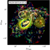 |
Fig. 1. Three-colour SPIRE image for G073.4−57.5 (reproduced from Planck Collaboration Int. XXVII 2015): blue, 250 μm; green, 350 μm; and red, 500 μm. The white contour shows the region encompassing 50% of the Planck flux density, while the yellow contours are the significance of the overdensity of red (350 μm) sources, plotted starting at 2σ with 1σ incremental steps. The rectangular area covering the ALMA pointings shown in Fig. 2 is highlighted in green. |
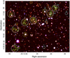 |
Fig. 2. Central region (5.8′ × 4.6′) of G073.4−57.5 in a 3-colour image of Spitzer-IRAC 3.6 μm (red), combined CFHT-WIRCam/VLT-HAWKI K-band (green) and J-band (blue), with Herschel-SPIRE 250 μm contours in yellow (from 0.02 Jy beam−1 in 0.0125 Jy beam−1 steps) and ALMA galaxy positions shown with green circles of radius 3″ (enlarged by a factor of 12 from ALMA’s synthesised beam for clarity), labelled according to their source IDs given in Table 2. The ALMA areas that were used for the analysis (0.2 times the primary-beam peak response) are indicated with white circles (37″ diameter), labelled according to their field IDs given in Table 2. Four SCUBA-2 sources centred in the cyan circles (13″ diameter, matching the beam size) are labelled according to MacKenzie et al. (2017); the two SCUBA-2 sources labelled “4+/5+” are additionally selected as > 3σ peaks in the SCUBA-2 maps coincident with ALMA-detected sources. ALMA field 5 (with one detected source, see Fig. 3) is located above and to the right of the central region and is not shown in this image. |
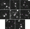 |
Fig. 3. Spitzer channel-2 postage stamps (30″ × 30″, with 2″ angular resolution) in grey scale (from 0.35 to 0.6 MJy sr−1) of the eight ALMA fields. White contours show the Herschel 250 μm surface brightness (from 0.01 Jy beam−1 in 0.005 Jy beam−1 or 1σ steps). Green contours represent the ALMA surface brightness (from 0.12 mJy beam−1 in 0.06 mJy beam−1 or 1σ steps). The detected ALMA galaxies are labelled with 1″ radius magenta circles, their photometric redshifts derived in Sect. 5 (or spectroscopic redshifts for ALMA IDs 3 and 8, Sect. 6) are given in white, and the ALMA fields are numbered in blue. |
3. ALMA observation of G073.4−57.5
We received 0.4 h of on-source observing time on G073.4−57.5 with ALMA in Cycle 2 (PID 2013.1.01173.S, PI R. Kneissl). We targeted the eight sources found in the SPIRE field that were consistent with a red colour, within the uncertainties, as defined above. A standard Band 6 continuum set-up around 233 GHz (1.3 mm) was used, with four 1.78 GHz spectral windows divided into the two receiver sidebands, separated by 16 GHz (i.e. central frequencies of 224, 226, 240, and 242 GHz). 34 antennas were available in the array configuration during the time of the observation, and the resulting synthesised beam achieved an angular resolution of 0.56″ × 0.44″ (FWHM) with a position angle of −82.7° (turning from north to east for a positive angle). The central sensitivity was approximately 0.06 mJy beam−1 in all eight fields (Fig. 2 for an overview, and we note the Herschel-SPIRE IDs, as given in Table 2); with this sensitivity ALMA can detect all SPIRE sources at any redshift, assuming a dust temperature > 25 K and that all the SPIRE flux comes from a single source, since the detection significance increases at higher redshifts. The observatory standard calibration was used. J2232+1143, a grid-monitoring source, was the bandpass calibrator and Ceres was observed as an additional flux calibrator. All pointings in this data set shared the same phase calibrator, J2306−0459. The single pointings were convolved with the primary-antenna-beam pattern (roughly Gaussian with a FWHM ≃ 25.3″, assuming 1.13 λ/D).
The data were reduced with standard CASA tasks (McMullin et al. 2007), including deconvolution, to yield calibrated continuum images with flat noise characteristics for source detection. A S/N > 5 mask was applied to the primary beam-uncorrected maps with a 2σ CLEAN threshold, yielding 13 sources in six fields, where the detection was based on the peak pixel surface brightness. In addition, the single brightest sources from each of the remaining two fields were included in the sample, since they were both well centred, with S/N > 4.5. During cross-matching with Spitzer maps, three additional sources were identified with S/N > 4.5. The final sample, containing 18 ALMA sources with flux densities > 0.3 mJy and S/N > 4.5, is presented in Table 1.
Basic properties of the ALMA galaxies detected at 1.3 mm in G073.4−57.5.
The flux-density results were derived from applying ImageFitter to the CLEANed maps and integrating over each source. They are presented in Table 1, along with the angular sizes for nine sources that were best fit with an extended profile (and four of which had a major axis determined with S/N > 3). In the nine remaining cases the fit for source size did not converge well and these are listed as point sources. In addition, we give the peak flux density at 233 GHz derived from the beam deconvolved map (which is more accurate for the nine point sources) and the coordinate for the position of the peak surface brightness. We note that ALMA source ID 16, which is on the edge of pointing field 7, has a recovered peak flux density of 0.59 ± 0.17 mJy beam−1, that is 3.5σ, and should thus be considered tentative, in spite of the match with a Spitzer source (cf. next section and Fig. 3).
4. Multi-waveband data
4.1. Dust spectral energy distributions
For the analysis of the SEDs of the far-infrared part of our multi-waveband data we used a modified black-body spectrum given by Lν = Nπa2Qν4πBν(T), where Qν ∝ ν β, Bν(T) is the Planck spectrum, N the number of grains, and a the grain size half-diameter (Hildebrand 1983)2. A submm dust opacity spectral index of β ≃ 2.0 is widely used, and lies within the range of theoretical models (Draine 2011), as well as empirical fits to nearby galaxies (e.g. Clements et al. 2010), and is close to the local interstellar medium (ISM) value (Planck Collaboration XXI 2011). In terms of the observed flux density3 this gives
![Mathematical equation: $$ \begin{aligned} S_{\nu } \propto \frac{N \nu ^{3+\beta } (1+z)^{4+\beta } D^{-2}_{\rm L}}{\mathrm{exp}[h \nu (1+z)/(k T_{\rm d})] - 1}, \end{aligned} $$](/articles/aa/full_html/2019/05/aa33252-18/aa33252-18-eq5.gif) (1)
(1)
where DL is the luminosity distance. Following Scoville et al. (2014, 2016) we can adopt a direct proportionality between the flux in the Rayleigh–Jeans regime and the ISM (i.e. H I, H2, and He) mass, with κν(ISM)/κν(dust) = MISM/Mdust (≃ 100). Then
 (2)
(2)
where x = 0.484(35 K/Td) (ν/353 GHz) (1 + z).
4.2. Herschel-SPIRE
G073.4−57.5 was observed with Herschel-SPIRE at 250, 350, and 500 μm (where the corresponding angular resolutions are 18″, 25″, and 36″, respectively) as part of the dedicated follow-up programme of 234 Planck sources (Planck Collaboration Int. XXVII 2015). The images reached 1σ (instrument + confusion) noise levels of 9.9 mJy at 250 μm, 9.3 mJy at 350 μm, and 10.7 mJy at 500 μm.
As discussed in the previous section, the SPIRE analysis revealed the presence of several red sources, compatible with a z ≃ 2 structure, centred approximately on SPIRE source ID 7 (i.e. ALMA field 3) and highly elongated in the NW-SE direction. A modified black-body fit of only the Herschel data for SPIRE sources 3, 7, and 15 (ALMA fields 2, 3, and 6) was consistent with z ≃ 2, assuming a dust temperature of Td = 35 K. Table 2 lists the SPIRE sources targeted with ALMA, along with their measured flux densities at 350 μm, the colours relative to 250 and 500 μm, and the sum per field of the 1.3 mm flux density resolved into the individual galaxies seen with ALMA.
Herschel-SPIRE sources observed with ALMA in the G073.4−57.5 field.
4.3. JCMT SCUBA-2
As part of a SCUBA-2 follow-up of 61 Planck high-z candidates (MacKenzie et al. 2017), G073.4−57.5 was observed at 850 μm with approximately 10′ diameter “daisy”-pattern scans, thus covering the whole Planck region. The imaging (with a matched filter applied) reached a minimum rms depth of 1.6 mJy beam−1. Table 3 lists the sources identified in MacKenzie et al. (2017), as well as their peak flux densities. These include all sources with S/N > 4 and within the Planck beam (i.e. the area in the Planck 353 GHz map, where the flux density was greater than half the peak flux density). We also include two additional sources that we have identified as having pronounced flux-density peaks coincident with the detected ALMA sources in fields 2 and 4, but with 3 < S/N < 4 in the SCUBA-2 data. These two additional, lower significance SCUBA-2 sources (labelled “4+” and “5+” in Table 3 and Fig. 2) are well matched to ALMA sources (although blended in the SCUBA-2 map). The apparent clustering of SCUBA-2 sources in Fig. 2 may indicate a physical concentration of bright submm sources around ALMA field 4. The ratios of the integrated flux densities, ALMA/SCUBA-2, for ALMA fields 2 and 4 are consistent with a modified black-body spectrum for z = 2.0, β = 2.0, and Td = 30 K. Conversely, for the other ALMA sources we would not necessarily expect strong individual detections in the SCUBA-2 data, given the sensitivity and confusion levels. Because of this we performed a stacking analysis by summing the flux densities in the matched-filtered SCUBA-2 maps at the positions of all the ALMA-detected mm sources, obtaining a significant signal of (56 ± 11) mJy, or (4.0 ± 0.5) mJy per source from a weighted average.
SCUBA-2 sources in G073.4−57.5.
4.4. Spitzer IRAC
G073.4−57.5 was observed with Spitzer-IRAC in GO11 (PID 80238, PI H. Dole), along with 19 other promising (i.e. high S/N and “red”) Planck sources with complimentary Herschel data. The observations involved a net integration time of 1200 s per (central) sky pixel at 3.6 μm (hereafter “channel 1”) and 4.5 μm (hereafter “channel 2”) over an area of about 5′ × 5′, and two additional side fields of the same area covered only in channel 1 or in channel 2. The area mapped in both channels with 2″ angular resolution is well matched to the angular size of one Planck beam and covers the full area of interest.
Source extraction in the IRAC mosaics was performed using SExtractor (Bertin & Arnouts 1996), with the IRAC-optimised parameters of Lacy et al. (2005). The detection threshold was set to 2σ. A choice was made not to filter the image due to the high density of sources. Photometry was performed using the SExtractor dual mode with the channel-2 mosaic as the detection image. Given the relative depth of channel 1 compared to channel 2, a detection at the longer wavelength can be sufficient to confirm that the source is red (i.e. selecting galaxies at z > 1.3, see Papovich 2008), where “red” in this context is defined as [3.6] − [4.5]> − 0.1 (in AB magnitudes). Aperture photometry was performed in a 2″ radius circular aperture, and aperture corrections were applied. The catalogues were then cut to 50% completeness in channel 2 (at 2.5 μJy). The surface density of IRAC red sources was computed in a circle of radius 1′ around SPIRE source ID 1 (which is the brightest red source in the Herschel-SPIRE field and central to the structure of bright Herschel sources selected for the ALMA pointings). The resulting surface density estimate is 14.6 arcmin−2. When compared to the field value derived from the Spitzer ultra deep survey (SpUDS) data at the same depth, which has a mean source density of 9.2 arcmin−2 (and a standard deviation of 2.2 arcmin−2), this corresponds to an overdensity of approximately 2.5σ (Martinache et al. 2018).
The ALMA detections have a match in at least the channel-2 image (Fig. 3), apart from galaxy ID 14, where there is emission in the Spitzer channel-2 map, but not significant enough to claim a detection. Most of the counterparts have a positional difference of d < 0.4″, except for three ALMA galaxies: ID 4 (0.6″); ID 16 (0.7″); and ID 15 (1.1″). In these cases the IRAC emission is seen to be extended (likely composites of two sources), with the ALMA source position still matching the detectable surface brightness of the IRAC source. It is also worth pointing out that these three galaxies (IDs 4, 15, and 16) match to blue IRAC sources. We note that the significant counterparts for ALMA IDs 2 and 7 appear weak in contrast to Fig. 3.
Searching for a stellar bump sequence (Muzzin et al. 2013) in the colour-magnitude diagram (Fig. 4) of sources lying in a circle of radius 1′ (balancing increasing numbers versus avoiding confusion) around SPIRE source 11, we found a median colour of IRAC red sources of 0.14 mag, and a dispersion of 0.15 mag. Most ALMA matches exhibit distinctly redder colours, with a median of 0.27 mag ([3.6] − [4.5]), and a dispersion of 0.13 mag. Such colours are compatible with a z ≃ 1.7 structure (Papovich 2008), but the scatter is high. SPIRE source 11 was chosen because it lies at the centre of an overdensity of IRAC sources (and indeed the majority of the SCUBA-2 detections are clustered around there, see Fig. 2).
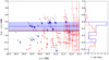 |
Fig. 4. Left: colour ([3.6] − [4.5]) versus magnitude ([4.5]) diagram for IRAC sources (red points) located within 1′ of SPIRE source 11, and for all the ALMA sources (blue stars); “[3.6]” means “channel 1” and “[4.5]” is “channel 2”. Numbers indicate the ALMA source IDs, as in Table 1. The black dashed line indicates a colour of −0.1 (red sources are defined to have colours above this value), the red line indicates the median colour of IRAC red sources within 1′ of SPIRE source 11 (0.14 mag), and the blue line indicates the median colour for the ALMA sources matched to IRAC red sources (0.27 mag). The dispersions around these median values are 0.15 and 0.13 mag, respectively (the latter is indicated by the blue region). The solid black line indicates the colour of a single stellar population formed at zf = 5, passively evolved to redshift z = 1.5 (from Bruzual & Charlot 2003), but extinction and possible metallicity effects have not been considered. Most ALMA sources lie on a sequence in this colour-magnitude plane, a characteristic feature of high-z structures (e.g. Muzzin et al. 2013; Rettura et al. 2014). We note that ALMA ID 14 is not plotted here, because it was not detected in the Spitzer-IRAC data. Right: normalised distribution of the colour of IRAC sources: the red line corresponds to sources within 1′ of SPIRE source 11; the blue line shows the ALMA sources; and the black dashed line shows the distribution of the colours of general sources in the COSMOS field for comparison. There is a significant excess of red galaxies around SPIRE source 11, in particular for the ALMA detections (further details in the text). |
Comparing the colour distributions shown in the right panel of Fig. 4 between ALMA sources, IRAC sources around SPIRE source 11, and all IRAC sources from the COSMOS field for reference, the Kolmogorov–Smirnov statistic gives large deviations (the highest for the ALMA sources versus the COSMOS sources) with probabilities less than 0.02 for the ALMA sources versus the IRAC sources around SPIRE source 11 and less than 2 × 10⁻⁵ relative to the IRAC sources from COSMOS; thus there is strong evidence that the sources are not drawn from the same distributions.
4.5. CFHT WIRCam J and K
G073.4−57.5 was observed by CFHT-WIRCam at 1.3 μm (J band) and 2.1 μm (Ks band) in projects PID 13BF12 and PID 14BF08 (PI H. Dole). The total integration times were 9854 s and 4475 s for the J and Ks bands, respectively. The area covered was 25′ × 25′, and the central 18′ × 19′ was selected in order to exclude the edges with high noise. For this analysis we extracted sources using SExtractor in dual mode with detection in the Ks band, reaching Klim = 22.94 ± 0.01 (AB, statistical error only) and Jlim = 24.01 ± 0.01, at a threshold level of 2.5σ (50% completeness). The completeness level was determined by placing 1000 simulated point sources at random positions, then using SExtractor to detect them and measure the percentage of recovered objects. By applying this procedure 10 times per filter, we derived the statistical error. The photometry was performed in a 2″ radius circular aperture and we applied the aperture correction in the same way as with the IRAC data. All sources flagged by SExtractor in the Ks band (except for blended ones), representing 11% of the catalogue, were removed from the analysis. We then matched the resulting catalogue with the 18 Spitzer-IRAC+ALMA sources and found 13 matches within 0.6″ (consistent with the seeing of the CFHT data). The five unmatched sources are IDs 1 and 10 (best match separation > 2.5″), and 2, 7, and 14 (not detected in Ks).
In Fig. 5 we summarise the evidence that the majority of ALMA sources lie at redshifts z ≃ 2 following the colour-redshift criteria of Papovich (2008) and Franx et al. (2003), and the evolutionary state predictions for a 1.4 Gyr simple stellar population (corresponding to a formation redshift zf = 3.5 for an observed redshift of z = 2, approximately applicable for the majority of the ALMA-detected galaxies). The galaxies with ALMA IDs 3, 5, 6, 8, and 9 appear to be more consistent with a redshift below 2, whereas the colours of IDs 11, 12, 13, 15, and possibly 17 seem to indicate redshifts above 2 (while having larger uncertainties). ALMA IDs 0, 4, and 16 may be interlopers at lower redshift (z ≤ 1).
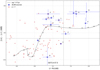 |
Fig. 5. Spitzer-IRAC versus CFHT WIRCam colour-colour diagram, with a track drawn from Bruzual & Charlot (2003) for a 1.4 Gyr simple stellar population, numbered by redshift. The horizontal and vertical dashed lines indicate the Papovich (2008) and Franx et al. (2003) criteria, respectively, representing colours of z ≃ 1.3 and z ≃ 2 galaxies (cf. the labels on the model curve). A redshift around z = 1.6–2.6 is indicated for the majority of the ALMA galaxies. Arrows represent 2σ limits for the sources not detected in any channel or band. |
4.6. WISE
Additional mid-IR data were obtained from the AllWISE catalogue (Wright et al. 2010; Mainzer et al. 2011) using a search radius of 3″. Six galaxies are detected in the W1 (3.4 μm) or W2 (4.5 μm) bands, one in the W3 (12 μm) band, and none in the W4 (22 μm) band (for details see Table A.1).
4.7. Pan-STARRS
We also searched the Pan-STARRS (grizy) DR1 data4 (Chambers et al. 2019), since even upper limits can provide additional constraints to the fits. The upper limits in AB mags are g = 23.3, r = 23.2, i = 23.1, z = 22.3, and y = 21.4. Only ALMA ID 4 is detected in the r, i, z, and y bands. The full set of available photometric data is reported in Table A.1.
4.8. VLA FIRST
A potential contribution from a radio-loud active galactic nucleus (AGN) can be investigated using the radio maps at 1.4 GHz of the VLA FIRST Survey (Becker et al. 1995). The 5σ threshold of the VLA FIRST survey, above which a point source is considered detected, is 0.75 mJy. Such a limit corresponds to an FIR luminosity ≥1013 L⊙ at redshift ≥1.5 for a radio-quiet AGN or a star-forming galaxy assuming a logarithmic FIR-to-radio luminosity ratio qIR = 2.4 and a radio slope αradio = −0.8 (Ivison et al. 2010). We find no strong evidence of flux at the positions of the ALMA galaxies. This is consistent with the estimated FIR luminosities (Table 5), which are all below such a value. We can thus affirm that none of the detected ALMA sources is a radio-loud AGN. The highest peak brightness of 0.62 mJy beam−1 is seen within the 5.4″ synthesised beam from the position of ALMA ID 12, but this is still below the detection threshold and consistent (log(LIR/L⊙)≲13.2 at z = 1.4 versus an estimated log(LIR/L⊙)=12.12 ± 0.06) with the FIR luminosity estimated for this source (Table 5). However, since radio-quiet AGNs and SFGs both lie on the FIR-to-radio relation, we cannot claim that the tentative radio detection of ALMA ID 12 is due to AGN or star-forming activity. Furthermore, the two ALMA galaxies, whose fit is consistent with an obscured AGN template are not ID 12.
5. Analysis
5.1. Source counts
Since we have targeted only the brightest Herschel sources found within this Planck peak, we can only make a qualitative comparison to known average ALMA mm source counts in order to discuss the approximate overdensity in sources of these regions.
Each ALMA field has been searched for sources within a 37″ diameter circle, over which the noise increases from the centre outwards by up to a factor of 5. The area of each field is 0.30 arcmin2, and adding together the eight fields we obtain a total survey area of 2.4 arcmin2, or 6.6 × 10⁻⁴ deg2. For the count estimate we take the eight sources in our sample with flux densities above 0.9 mJy. The effective area over which these sources can be detected is 75% of the total (i.e. where rms is < Sν / (S/N) = 0.9 mJy / 4.5 = 0.2 mJy). Thus, the surface density is 8 / (0.75 × 6.6 × 10−4 deg2) = 1.6 × 10⁴ deg−2.
Comparing to recent blank-field counts of ALMA sources (e.g. Hatsukade et al. 2016; Dunlop et al. 2017), serendipitous counts derived from various archival data (e.g. Hatsukade et al. 2013; Ono et al. 2014; Carniani et al. 2015; Oteo et al. 2016; Fujimoto et al. 2016), or source numbers found in lensing cluster fields (e.g. González-López et al. 2016; Muñoz Arancibia et al. 2018), we estimate an expected 1.2 mm source density of 0.6–2 × 10³ deg−2, where the lower estimate (from Oteo et al. 2016) is derived from a relatively large area of different fields used for the serendipitous searches, which might be expected to reach beyond the effects of cosmic variance. Thus, the number of sources we find in the ALMA pointings of G073.4−57.5 is a factor of 8–30 higher than estimates of the average number of mm sources in the sky.
In terms of the total numbers of mm/submm sources in the G073.4−57.5 field, 18 are identified with ALMA (even without a complete mosaic of the total emission region of the Planck/Herschel peak), and an additional four from SCUBA-2, for a total of 22 mm/submm sources in the area of the Planck peak. In comparison, typical “proto-cluster” overdensities, not selected by their high integrated submm flux, do not show the same abundance. Examples include the COSMOS z = 2.47 structure (Casey et al. 2013, 2015) and the SSA22 z = 3.09 structure (Chapman et al. 2001; Umehata et al. 2015), each of which contains 12 sources (Casey 2016, in particular their Table 1, for a comprehensive summary of SFGs in several overdense regions) at a comparable depth, although the SCUBA-2 850 μm data for the COSMOS structure are not as deep, at 0.8 mJy rms (Casey et al. 2013). In a more recent study of the SSA22 structure Umehata et al. (2017) find 18 ALMA sources (> 5σ) at 1.1 mm, but over an area of 2′ × 3′ and with a depth of 0.06–0.1 mJy, much wider and overall somewhat deeper (given their shorter wavelength and homogeneous coverage) than our data, requiring approximately 16 times our on-source time with comparable numbers of antennas and conditions. At a similar depth and area to our selected eight pointings, this would correspond to about four detections. A comparison with the z = 1.46 cluster XCS J2215.9−1738 studied by Stach et al. (2017) with the same ALMA on-source time in a 1 arcmin2 central mosaic shows a similar number of sources (14, with 12 likely members), but they are all weaker (< 1 mJy). They find a total SFR of 850 M⊙ yr−1, which is lower than the ≳2700 M⊙ yr−1 in our sample (cf. Sect. 5). The SCUBA-2 sources in XCS J2215.9−1738 break up mostly into groups of two to three ALMA sources, similar to the SCUBA-2 and Herschel sources in G073.4−57.5. The early (z = 4.00) proto-cluster found by Oteo et al. (2018) with 10 galaxies, on the other hand, has a higher SFR of ≳6500 M⊙ yr−1.
We can conclude that for our data, contamination by the average background source is expected to be small, amounting to about one to three galaxies not related to the structure(s) causing the Planck peak. We discuss later whether gravitational lensing could affect the number counts.
5.2. Spectral energy distributions and photometric redshifts
The detection, in most cases, of several ALMA galaxies (with sub-arcsecond accuracy) per single Herschel target allows us to employ a deblending technique to estimate the Herschel-SPIRE fluxes of these galaxies, which can then be used to fit SEDs and derive several physical properties. To accomplish this we use a combination of a recently developed algorithm called SEDeblend (MacKenzie et al. 2017), specifically designed for confused FIR imaging, and the EAZY code (Brammer et al. 2008), to estimate source photometric redshifts and find the best fits to their multi-wavelength SEDs.
We first applied EAZY to all available flux measurements for each source (excluding those from Herschel-SPIRE, which are initially too confused to be useful) to obtain posterior probability distributions for photometric redshifts. For the 850 μm data from SCUBA-2, the flux density from SCUBA-2 ID 4+ was assigned proportionally to the ALMA flux of IDs 2 and 4 (ID 3 also falls into field 2, but is 11″ from the SCUBA-2 position, see Fig. 2), and the flux density from SCUBA-2 ID 5+ was assigned proportionally to ALMA IDs 8 and 9. Similarly, the Herschel-SPIRE flux densities were initially assigned according to the ALMA flux-density ratios of the constituent galaxies. The library of SED templates employed by EAZY covers the full optical–mm spectral range and a wide variety of galaxy types, including early-type galaxies, SFGs, SBs, AGNs, and SMGs, for a total of 37 templates (23 from the SWIRE library, and 14 from the zLESS compilation, Polletta et al. 2007; Danielson et al. 2017).
We then used the resulting photometric redshift posterior probability distributions as inputs to SEDeblend. To summarise briefly, SEDeblend reconstructs the Herschel-SPIRE 250 μm, 350 μm, and 500 μm images and the SCUBA-2 850 μm image by placing a point source multiplied by the appropriate instrumental point-spread function at each location of a detected ALMA galaxy and adding a constant background offset, then uses a Markov chain technique to simultaneously fit for galaxy SED parameters. The ALMA images were not reconstructed, since the much greater angular resolution there, after CLEANing, leads to essentially no source blending. The model takes into account each Herschel-SPIRE instrumental transmission function (typically amounting to a 10% flux correction), and considers calibration uncertainties by multiplying the flux in each band by a nuisance parameter, whose prior is a Gaussian function with a mean of 1.0 and a standard deviation given by each instrument’s quoted calibration uncertainty. The SEDs are modelled as modified black-bodies (Eq. (1)) at a redshift z with a temperature Td, an overall normalisation constant, and the dust emissivity-index is fixed at β = 2.0. For more details on SEDeblend we refer to MacKenzie et al. (2017).
For the fitting, a Markov chain Monte Carlo (MCMC) algorithm with Gibbs sampling and adaptive step-sizing was used to maximise a Gaussian likelihood function calculated pixel-by-pixel for the SPIRE and SCUBA-2 images, and source-by-source for the ALMA flux measurements. The chain was run for 120 000 iterations and the first 20 000 iterations were removed as the “burn-in” sequence. We set a sufficiently wide uniform prior on the amplitudes of the modified black-body SEDs and the background levels to leave them effectively unconstrained, and a uniform prior between 10 and 100 K on the dust temperatures (since no galaxies have been observed to lie outside this range, e.g. Dale et al. 2012; Swinbank et al. 2014). To remove the degeneracy between temperature and redshift in the modified black-body model, the photometric redshift posterior probability distributions from EAZY in the previous step were input as the prior for the new photometric redshifts.
From the resulting Markov chain we derived the Herschel-SPIRE flux densities in each band by evaluating Sν(νb), with b labelling the band, from each iteration within the MCMC algorithm (thus obtaining the marginal likelihood) and calculate the maximum likelihood and 68% confidence interval; these are reported in Table 4. In a few cases the 68% confidence interval extends to 0 mJy (IDs 11, 15, and 16). For these cases, and when the measured flux is < 2σ, we assigned an upper limit equal to the maximum likelihood flux plus 3σ. In the SED fitting procedure and in Fig. A.1 we also considered the SPIRE confusion limits (i.e. 5.8, 6.3, and 6.8 mJy at 250, 350, and 500 μm, respectively; Nguyen et al. 2010) when dealing with upper limits. For consistency, we check the mm/submm properties (such as dust temperature, FIR luminosity, and SFR, discussed in the following section) derived from SEDeblend with those derived in Sect. 5.3 and find them to be in generally good agreement.
Deblended SCUBA-2 and Herschel-SPIRE flux densities for the individual ALMA-detected galaxies.
We lastly re-ran EAZY with the now deblended Herschel-SPIRE and SCUBA-2 flux densities included. The best-fit templates and SEDs are shown in Fig. A.1, and photometric redshifts and associated uncertainties are listed in Table 5. The redshift uncertainties correspond to the range of redshifts with a probability higher than half the maximum value.
Best-fit SED parameters and 1σ uncertainties.
Reasonably good fits (median  ) are obtained for most of the galaxies, with the exception of IDs 14 and 16. For these sources, which are found in ALMA region 7, it seems plausible that the source blending is simply too substantial to be overcome; four galaxies are sharing a combined flux half that of most of the other regions, where there are three or fewer galaxies. We thus suggest caution in the interpretation of galaxies 13 through 16.
We also note that the two galaxies within region 4, IDs 8 and 9, are the most closely-spaced pair in the data, separated by less than a pixel in the SPIRE maps. This leads to strong degeneracies between the best-fit SED parameters found by SEDeblend, which may result in unreliable flux estimates. However, the redshift derived by our procedure for galaxy 8, z ≃ 1.3, is similar to the ALMA CO spectroscopic redshift (details in Sect. 6).
The best-fit templates selected by EAZY for all of our sources come from the zLESS library, with only three exceptions, where a template is from the SWIRE library. In one of these three cases (ID 14), the best-fit template corresponds to the prototypical ULIRG Arp 220, and is thus similar to those in the zLESS library. The presence of a significant FIR peak and red optical colours probably favour this type of template compared to those of passive, spiral, and starburst galaxies. In another case (ID 6), the best-fit template corresponds to Mrk 231, another well-known ULIRG that contains an obscured AGN, and in the final case (ID 15) the best-fit template is that of an obscured Seyfert galaxy. IDs 6 and 15 are among the reddest sources in the [3.6] − [4.5] colour, implying that the peak of the stellar component (at 1.6 μm in the rest-frame, Sawicki 2002) must be redshifted to λ> 4.5 μm, unless an AGN-heated hot dust component contributes to their mid-IR emission. In the case of ID 6 the FIR SED implies a redshift z ≲ 1.5; in order to fit both the red IRAC colour and the FIR SED, an AGN template is favoured, since it can reproduce the red IRAC colour through the contribution of a hot dust component. The FIR SED of ID 15 is not very well constrained, but its relatively low emission compared to the NIR emission, as well as its extremely red colours, favour a hybrid template where both the stellar and AGN components are visible; however, a starburst template at approximately the same redshift yields a similarly good fit, so the presence of an AGN in this source is uncertain.
We validate our photometric redshifts by first checking the SCUBA-2 flux densities predicted for all ALMA galaxies based on the fits. We find that our best-fit SEDs give a total SCUBA-2 flux of 58 mJy, in good agreement with the stacking result of (56 ± 11) mJy.
The photometric redshift distribution of all ALMA sources is shown in Fig. 6, along with the combined probability distribution function (PDF), that is the sum of the likelihoods output from EAZY. Both the single photo-z distribution and the combined PDF of the ALMA sources show two redshift concentrations, one at z ≃ 1.5 and the other at z ≃ 2.4 (vertical dashed lines in Fig. 6). The redshift distribution suggests that G073.4−57.5 might contain two structures overlapping along the line of sight.
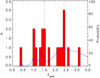 |
Fig. 6. Photometric redshift distribution of the maximum-likelihood solutions (filled red histogram) and combined probability density function (PDF, i.e. sum of the individual source likelihoods; solid blue curve) obtained with EAZY for all ALMA galaxies in the G073.4−57.5 field. Both the single photo-z distribution and the combined PDF of the ALMA sources show two clear redshift concentrations, one at z ≃ 1.5 and the other at z ≃ 2.4 (indicated by the vertical dashed lines). |
5.3. FIR-derived parameters
The total (8–1000 μm) IR luminosities (LIR), dust masses (Md), dust temperatures (Td), and SFRs of our ALMA sources were estimated by fitting their FIR-mm SEDs with single-temperature modified black-body models. Fits were performed using the cmcirsed package (Casey 2012) and assuming the photometric redshifts derived above (or, when available, the CO spectroscopic redshifts, see Sect. 6) and a dust emissivity-index β equal to 2.0 (Pokhrel et al. 2016, see the purple curve in Fig. A.1). Uncertainties on LIR and Td were derived by fitting the SPIRE data and assuming the SPIRE flux plus (minus) 1σ at 250 μm and the ALMA flux plus (minus) 1σ at 233 GHz to obtain the best-fit with the highest (lowest) temperature. These two best fits are shown as red (warmest) and cyan (coldest) dashed curves in Fig. A.1, respectively. From the IR luminosities, SFR estimates were derived assuming the relationship in Kennicutt (1998), modified for a Chabrier initial mass function (IMF) (Chabrier 2003), that is SFR[M⊙ yr−1] = 9.5 × 10⁻¹¹ LIR[L⊙].
The FIR-derived parameters LIR, Md, Td, and SFR are listed in Table 5. The majority (≳70%) of the ALMA galaxies are classified as ULIRGs (LIR ≥ 1012 L⊙; Sanders et al. 1988), with consequently large (≳100 M⊙ yr−1) SFRs. The highest SFRs (> 300 M⊙ yr−1) are measured in IDs 8 (zCO = 1.5449, see Sect. 6), and 1 ( ). In Sect. 5.4 we find that, in spite of the large SFRs, most ALMA galaxies lie on the SFR–ℳ MS (Speagle et al. 2014). The dust temperatures, with an average of ⟨Td⟩ = (27 ± 5) K, are within the expected range for normal SFGs at z ≳ 1 (Magnelli et al. 2014), and the dust masses are within the expected range of 108 − 109 M⊙ (Popping et al. 2017; Rémy-Ruyer et al. 2014).
In order to estimate stellar masses we fit only the Pan-STARRS-WIRCam-IRAC SED, fixing the redshift to the photo-z or to the spec-z, when available, using the Hyper−z code (Bolzonella et al. 2000) and the composite stellar population models from Bruzual & Charlot (2003), then assuming a Chabrier IMF. The estimated stellar masses are also listed in Table 5. The reported uncertainties are likely to underestimated because they do not take into account the redshift uncertainty or the choice of IMF, synthetic models, and fitting method (e.g. Kannappan & Gawiser 2007; Barro et al. 2011). In addition, the reported uncertainties are obtained from the best-fit template and do not consider the likelihoods associated with the full set of models (i.e. full PDF). We thus caution using these stellar masses, especially when the uncertainties are less than 0.1 dex. In the following analysis we use these estimates only to compare our sources with well known relations from the literature. The scatter associated with these relations is likely to be larger than the neglected additional uncertainties, and moreover the systematic uncertainties are less important when considering relative measurements, so that our interpretations should still be valid. In the next section we compare the estimated stellar masses and SFRs of our ALMA galaxies to those of typical SFGs.
5.4. Relationship to main-sequence galaxies
In Fig. 7, we compare the derived stellar masses with the expected values of the characteristic mass ℳ* obtained by fitting the Schechter mass function of SFGs in multiple redshift intervals between 0.2 and 4.0 (Davidzon et al. 2017). Nine ALMA galaxies have stellar masses comparable with the expected ℳ* values, the other nine galaxies are instead more massive than the expected ℳ* values, with stellar masses above 3 × 10¹¹ M⊙, implying that they have become quite massive early on.
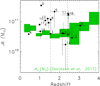 |
Fig. 7. Stellar mass as a function of photometric redshift for the 18 ALMA galaxies. The green rectangles represent the expected values of the characteristic mass ℳ* and their uncertainties obtained by fitting the mass function of SFGs with a Schechter function in the redshift ranges 0.2–0.5, 0.5–0.8, 0.8–1.1, 1.1–1.5, 1.5–2.0, 2.0–2.5, 2.5–3.0, 3.0–3.5, and 3.5–4.0 (Davidzon et al. 2017). The source IDs are labelled next to the corresponding symbols. |
In Fig. 8, we show the location of our sources with respect to the MS relation. To accentuate the offset from the MS (i.e. the “starburstiness”) for our ALMA galaxies, we plot the IR-derived SFR normalised by the expected SFR based on the MS at each source redshift, as parameterised by Speagle et al. (2014), as a function of redshift. The grey region corresponds to the scatter around the MS, which is about a factor of 3. The majority (13 out of 18, or 72%) of our ALMA galaxies lie within this factor of 3 of the main sequence, while two ALMA galaxies lie below this region (IDs 15 and 16) and three lie above it (IDs 1, 8, and 14). These latter three sources (where it must be noted that the SFRs derived for ID 14 may not be reliable) are thus experiencing enhanced star-forming activity, consistent with being SB galaxies. It is indeed typically assumed that SB galaxies are offset by a factor of ≃3–4 or more from the MS (Elbaz et al. 2011; Rodighiero et al. 2011).
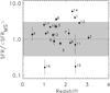 |
Fig. 8. “Starburstiness”, which is the ratio of the star-formation rate to the SFR expected for a source on the MS (using the relation at the respective redshift), plotted against redshift. A factor of 3 around the MS is indicated by the grey region. Stars highlight galaxies assumed to be at z ≃ 1.54. |
From this analysis, we notice the following. Firstly, the sources in the redshift concentration around z ≃ 1.5 (IDs 3, 5, 6, 8, and 12, shown as large stars in Fig. 8) are mostly on the MS and more massive than the expected ℳ*. Conversely, there is a group of three galaxies (IDs 1, 13, and 14) around z ≃ 2.3–2.6, corresponding to the second most prominent redshift concentration (Fig. 6), with large starburstiness values (SFR ≥ 3 × SFRMS), but stellar masses consistent with or below the expected ℳ*. These two redshift concentrations might be associated with two structures, one in the background, at z ≃ 2.4, where galaxies are actively forming stars and are still building their stellar masses, and one in the foreground, at z ≃ 1.5, where most galaxies have reached the end of their stellar mass build-up and their activity level is relatively low. Finally, we note that the most massive galaxies (IDs 0, 5, 11, and 15) are on the MS, or below it, as expected for objects close to the end of their active phase. Two of these galaxies are at z ≃ 2.4 and might thus be in the same structure as IDs 1, 13, and 14. If true, then we would have two types of member of the z ≃ 2.4 structure: one starbursting, with less-than-expected stellar mass (IDs 1, 13, and 14); and the other lying on or below the MS and with greater-than-expected stellar mass (IDs 11 and 15).
The total SFRs of these two structures are 840 yr−1 and 1020
 yr−1 for the z ≃ 1.5 and z ≃ 2.4 structures, respectively, and the associated total stellar masses are (5.8
 and (4.2
 . These numbers yield starburstiness values of 2.4, and 1.9, respectively, thus consistent with the MS at their redshifts.
6. Serendipitous line detections
6.1. ALMA galaxies ID 3 and 8
Spectral cubes of the ALMA primary-beam-convolved continuum (128 channels for each of the four 2 GHz wide spectral windows) were made for the eight fields, with a spectral binning of width 0.08 GHz, giving 25 frames, for the line search. The spectra were analysed in the local standard of rest (kinematic, i.e. LSRK) with 64 frames per spectral window. Fluxes quoted in the text are beam corrected.
ALMA galaxy ID 3, the brightest mm galaxy located in ALMA field 2, shows the detection of a strong line at (226.656 ± 0.009) GHz (line peak in Fig. 9, top panel). We find an integrated flux density of (2.5 ± 0.2) Jy km s−1 beam−1 at the spatial peak, and (2.9 ± 0.2) Jy km s−1 in an extended aperture (Fig. 10), with a line width of (417 ± 31) km s−1 for the FWHM in the Gaussian fit (Table 6). Using the physical size of this source as 0.44″, the semi-major axis from Table 1, the dynamical mass can be estimated as Mdyn = (417 km s−1)2 × 3.8 kpc / G = 1.5 × 10¹¹ M⊙, as compared to a stellar mass of  (from Table 5).
Spectral fitting results for ALMA galaxies IDs 3 and 8.
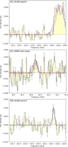 |
Fig. 9. Spectra of the two ALMA galaxies ID 3 (top and middle) and ID 8 (bottom), showing the serendipitous line detections, consistent with a CO(5–4) transition at z = 1.54. The blue Gaussian profiles show the best fits to each individual line. The red Gaussian profiles for ID 3 show the best combined fit to the CO(5–4) line in the ALMA spectrum (top) and the CO(2–1) line in the IRAM/EMIR spectrum (middle). The offset between the fitted line centres seen in the EMIR data is small, 66 km s−1, and could be due to the low S/N, the edge of the ALMA spectral window, or a physical difference between the transitions. Representative error bars per bin are shown for every third bin. We note that we have applied the standard flagging of edge channels in the ALMA spectral window for ID 3, which otherwise could introduce systematic uncertainties. |
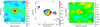 |
Fig. 10. Images for ID 3 (on the left) and ID 8 (on the right) of the integrated line emission in Jy km s−1 beam−1 (where the continuum has been subtracted). In both cases line and continuum emission (i.e. the black contours from 3σ = 0.18 mJy in 3σ steps) coincide. The middle panel shows (for the stronger line of ID 3 only) the first-moment image in km s−1, along with continuum contours for reference. The FWHM of the synthesised beam (0.56″ × 0.44″) is shown with red ellipses and a 5 kpc bar is shown in black for reference. |
The galaxy shows a smooth velocity gradient from north-east to south-west (Fig. 10, middle panel), but it is only barely resolved spatially. CO transitions are known to be bright for mm and submm galaxies (e.g. Carilli & Walter 2013; Vieira et al. 2013), and would correspond to the redshifts z = 1.034 CO(4–3), 1.542 for CO(5–4), 2.051 for CO(6–5), and 2.559 for CO(7–6), if we keep with the most plausible range of z ≃ 1–3.
Associating the observed line with the CO(5–4) transition appears the most plausible conclusion, since it provides the closest match for the photometric redshift of ALMA galaxy ID 3. However, we now briefly discuss other interpretations. The higher redshift transitions (J > 6, corresponding to z > 2.5) would yield poorer agreement with the photometric redshifts, and in addition may be expected to be much weaker. The C I(2–1) line would provide a direct identification, as its rest frequency of 809.34 GHz is very close to the rest frequency of the CO(7–6) line, which has a rest frequency of 806.65 GHz; however, this is not possible with our observation, since the expected 227.4 GHz (sky frequency) line would lie inside the sideband separation. Moreover, a redshift around z ≃ 1 does not seem consistent with the colour and photo-z results of most of our galaxies (apart from those identified as interlopers). On the other hand, CO(6–5) appears possible, though not favoured by the photometric redshifts within their errors.
6.2. IRAM-30m/EMIR CO redshift
Observations of G073.4−57.5 were carried out using the heterodyne receiver EMIR (Carter et al. 2012) on the IRAM 30-m telescope between 13 and 16 September 2016 (PID 077-16, PI C. Martinache). We used the 3 mm band (E090) to search for CO transitions. The frequencies covered were 74–82 GHz and 90–98 GHz. For the backends, we simultaneously used the wideband line multiple autocorrelator (WILMA, 2-MHz spectral resolution) and the fast Fourier transform spectrometer (FTS200, 200-kHz resolution). Given that the observed object, SPIRE source 3 (ALMA field 2, see Table 2), is a point source, observations were performed in wobbler-switching mode with a throw of 30″. The FWHM of IRAM 30-m/EMIR is 27″ at 91 GHz, comparable to the Herschel-SPIRE beam at 350 μm (25″). The total integration time was 300 min. For calibration, pointing, and focusing we used Jupiter, Mars, and bright quasars. Data reduction was performed with the help of the CLASS package in GILDAS (Gildas Team 2013). Baseline-removed spectra were co-added using the inverses of the squares of the individual noise levels as weights. We then fit the co-added spectra with a Gaussian profile and derived the line position, the peak flux, and the line width (FHWM). The results are presented in Table 6.
In Fig. 9, middle panel, we show the EMIR spectrum, together with the best-fit Gaussian curves for the EMIR data and the combined EMIR and ALMA data. We note a significant (4.7σ) detection very close (90 km s−1 separation) to the expected frequency of 90.674 GHz for the CO(2–1) transition. We take the EMIR spectrum and the joint fit result as a strong indication for a CO(5–4) line in ALMA and a redshift of z = 1.5423 ± 0.0001 (Table 6); this is dominated by the high S/N ratio in the ALMA data (fitted Gaussian curves in Fig. 9, top panel). We assume, of course, that the EMIR line comes from ALMA ID 3 and not from another galaxy within the larger beam, and also not from another molecular species, since either of these options would be a rather unlikely coincidence.
6.3. CO line properties
Under the assumption that the detected line in ALMA is indeed CO(5–4), the CO luminosity can be calculated as (Solomon et al. 1997)
 (3)
(3)
Using the linewidth estimate and peak intensity from the joint fit (Table 6), we find  K km s−1 pc2, consistent with the integrated line flux density of Fig. 10. The CO(2–1) luminosity for the EMIR line, also using the joint fit results, is
  K km s−1 pc2, giving a ratio of r54/21 = 0.36 relative to the CO(5–4) transition luminosity, consistent with the values measured for typical SMGs (e.g. Carilli & Walter 2013). We also find tentative evidence for a faint line (S/N ≃ 4.4 over four channels with two-channel Hanning smoothing) in ALMA galaxy ID 8 (the brightest detection in ALMA field 4), which has very similar NIR properties to those of ALMA galaxy ID 3 (Figs. 4 and 5). There is a (spatially unresolved) peak of intensity (0.274 ± 0.062) Jy km s−1 at (226.474 ± 0.004) GHz in Fig. 10. In the Gaussian fit the linewidth is (101 ± 31) km s−1 (Table 6), and the redshift is z = 1.54452 ± 0.00004 for the same CO(5–4) transition. Using the parameters of the fit the line luminosity is
  . The dynamical mass estimate is Mdyn = 9.2 × 10⁹ M⊙, that is much smaller than the expected stellar mass of ℳ = 1.1 × 10¹¹ M⊙ (from Table 5). The near coincidence of the frequency with that of ID 3 argues for the reality of this weaker line.
For these two galaxies, with the simple assumptions that  , with r54/10 = 0.32 ± 0.05 (the median brightness temperature ratio derived for SMGs by Bothwell et al. 2013), we derive gas masses of (4.7 ± 0.8) αCO × 1010 M⊙ (ID 3) and (3.5 ± 1.5) αCO × 109 M⊙ (ID 8). Assuming αCO = 4.36 M⊙ / (K km s−1 pc2), more typical of an MS galaxy (Bolatto et al. 2013), Mgas = (2.0 ± 0.4) × 1011 M⊙ (ID 3), and (1.5 ± 0.6) × 1010 M⊙ (ID 8); on the other hand, αCO = 0.8 M⊙ / (K km s−1 pc2), more typical for SB galaxies (Solomon et al. 1997), yields (3.7 ± 0.7) × 1010 M⊙ (ID 3), and (2.8 ± 1.2) × 109 M⊙ (ID 8). However, the large difference in the assumed conversion factors also indicates that there is a range of uncertainty.
The gas content and star-formation efficiency (SFE) of galaxies in high-redshift overdensities are of great interest, since they allow us to constrain the mechanisms that trigger, regulate, and quench their star-formation activity. In addition, a comparison with galaxies in the field, in clusters, and in other proto-clusters can provide insights into the role played by the environment. To this end, we collected CO data from the literature for galaxies in clusters (62 galaxies in 11 clusters, Wang et al. 2018; Rudnick et al. 2017; Stach et al. 2017; Aravena et al. 2012; Casasola et al. 2013; Castignani et al. 2018; Coogan et al. 2018; Hayashi et al. 2017; Webb et al. 2017) and in proto-clusters (16 galaxies in four proto-clusters, Dannerbauer et al. 2017; Ivison et al. 2013; Tadaki et al. 2014; Lee et al. 2017), and of SMGs and AGN in the z = 1–3 redshift range (31 SMGs, 15 AGN, and 38 obscured AGN, Perna et al. 2018). In order to represent normal star-forming galaxies and SB galaxies, we used the SFR–ℳ relation5 from Speagle et al. (2014), and the  relation from MS and SB galaxies as derived by Sargent et al. (2014)6
For estimating molecular gas masses, we converted all high transition CO luminosities to  , when not available, using the median brightness temperature ratios derived by Bothwell et al. (2013). In order to investigate the gas fractions, we considered only the cluster and proto-cluster galaxies for which a stellar-mass estimate was available (14 clusters galaxies and 14 proto-cluster galaxies). Extending the molecular gas analysis to all of our ALMA-detected galaxies, we also considered ISM masses estimated from the mm continuum at 233 GHz by applying Eq. (2) (Scoville et al. 2016, see Table 5). This method, based on the continuum level of the Rayleigh–Jeans tail associated with the ISM thermal emission, is limited to galaxies within a certain redshift and mass range and for limited dust temperatures, but is less affected by the CO kinematics, clumpiness, and metallicity that affects the CO excitation level (Scoville et al. 2014, 2016). In the following analysis, we consider gas masses derived from the CO line for ALMA IDs 3 and 8, and ISM masses derived from the ALMA continuum for all of the ALMA sources.
In Fig. 11, we show the SFE, defined as the ratio between LIR (which is proportional to the SFR) and  (which is proportional to Mgas), as a function of LIR for all of the examples from the literature, as well as ALMA IDs 3 and 8. We also show the expected SFE for main sequence and starburst galaxies as derived from Eqs. (5) and (6). The SFEs of field SMGs, AGN, obscured AGN, and proto-cluster galaxies are consistent with either the MS or the SB relation. Cluster galaxies exhibit, on average, smaller IR luminosities than the other sub-samples, and their SFEs cover a wider range, from 0.8 dex lower to 0.9 dex higher than the expected MS values. The two galaxies detected by ALMA in CO show different behaviour: the SFE of ID 3 is 0.36 dex lower than expected according to the MS relation; but, on the other hand, the SFE of ID 8 is among the highest observed, 0.65 dex higher than the SB-expected value.
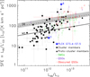 |
Fig. 11. SFE (≡ |

SFE is inversely proportional to the gas depletion time, modulo a normalisation factor that depends on the value of αCO, that is  . In this paper, we prefer not to discuss the gas depletion times because this definition does not take into account the variety of processes (gas accretion and removal) that might be relevant in overdense environments, and thus the estimated values might be misleading. We instead examine the SFE as defined here and compare it with the values reported in the literature. As a reference for guidance, we note that SFE values consistent or above the expected SB values (Fig. 12) would imply fast depletion times, consistent with bursty star-formation activity (τdepl < 100 Myr), while SFE values consistent with the MS are longer and consistent with secular evolution (between 0.5 and 1.5 Gyr).
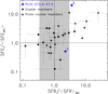 |
Fig. 12. SFE normalised to the expected SFE assuming the relation valid for MS galaxies from Eq. (5) as a function of offset from the MS (starburstiness) for ALMA IDs 3 and 8 (filled stars), and for sources from the literature with 1 < z < 3 (filled squares: cluster galaxies, filled triangles: proto-cluster galaxies). The horizontal and vertical solid lines represent, respectively, SFEs and starburstiness values of MS galaxies, and the grey region indicates SFRs consistent with the MS within a factor of 3. |
The wide range of SFEs in cluster galaxies could be due to processes that favour star formation, such as gas accretion and cooling, or that hamper it through gas removal or heating. Molecular gas studies of high-redshift clusters show a significant suppression of molecular gas for all the massive cluster galaxies close to the centre (within the core radius). This indicates that the environment plays a role in stopping gas accretion and/or reducing/removing gas content (Hayashi et al. 2017; Wang et al. 2018; Foltz et al. 2018; Socolovsky et al. 2018; Castignani et al. 2019). On the other hand, ALMA observations of the proto-cluster 4C23.56 at z = 2.49 (see Lee et al. 2017) suggest gas masses and fractions of its members consistent with those of field galaxies, implying a higher gas density in the proto-clusters than in the field by an order of magnitude, due to the overdensity.
In the rest of this section, we investigate whether this is also true for the ALMA-detected galaxies by comparing their molecular gas content with the expected values for MS and SB galaxies (see Sargent et al. 2014), and with those observed in other cluster and proto-cluster members for which both CO and stellar masses are available.
In Fig. 13 we show the molecular gas mass derived using CO luminosities for ALMA IDs 3 and 8, cluster galaxies, and proto-cluster galaxies, as a function of LIR, and the expected values for MS or SB galaxies (Sargent et al. 2014). Gas masses are derived using  . The adopted αCO value for each galaxy is that reported in earlier studies (Tadaki et al. 2014; Dannerbauer et al. 2017; Wang et al. 2018; Lee et al. 2017; Ivison et al. 2013), and had been fixed to either αCO = 0.8, typical of SB galaxies, or αCO = 4.0–4.36, typical of normal SFGs. We remind that we consider as an SB any source with SFR > 3 × SFRMS, but this definition might not match what was found in other published samples. In the case of our CO-detected sources, ALMA IDs 3 and 8, we show gas masses assuming both αCO = 0.8, and 4.36. We also show the full ALMA sample assuming that MISM is equivalent to the gas mass (see Eq. (2), Scoville et al. 2016). Most of the objects are within a factor of 3 from the expected relations (Sargent et al. 2014), with a few exceptions that are either richer or poorer in gas. For our selection of galaxies in the mm range, the ISM mass estimates of the ALMA galaxies are scattered around the MS relation (mostly above), similar to the galaxies from the literature. ALMA ID 3 is richer in gas than expected from the relations for either MS or SB galaxies with the respectively assumed αCO values. The ISM mass estimate is similar (within 2σ7) to the molecular gas mass derived from the CO line assuming αCO = 4.36. Thus a line ratio CO(5–4)/CO(1–0) of r54/10 ≃ 0.3, as indicated also by the EMIR data and assumed here (e.g. r54/21 = 0.38 in Bothwell et al. 2013), and an αCO of 4.36 (as for spiral galaxies, see Bolatto et al. 2013), are plausible for ID 3, since they bring the gas CO and ISM mass estimates into agreement. This suggests that the molecular gas in ID 3 has properties similar to that of SMGs. The molecular gas derived from the CO line in ID 8 is instead significantly lower than expected for both an MS or an SB galaxy, while its ISM mass falls exactly on the MS relation. This discrepancy suggests that the assumed CO excitation might not be adequate for this source. Indeed it is well known that there are large uncertainties involved with the conversion factors (see e.g. Daddi et al. 2015, for CO excitations), up to perhaps a factor of 5.
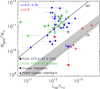 |
Fig. 13. Molecular gas mass, derived from the CO luminosity (in red if αCO = 0.8, and in blue if αCO = 4.0–4.36), as a function of LIR for ALMA IDs 3 and 8 (filled stars) and galaxies in clusters (filled squares) or in proto-clusters (filled triangles). Gas masses refer to ISM masses derived from the mm continuum for all ALMA sources (green open stars with annotated IDs). The solid and dashed lines represent the expected relations for MS and SB galaxies, respectively, as derived from Eqs. (5) and (6), and assuming αCO = 4.36 (for MS galaxies) or 0.8 (for SB galaxies, SFR > 3 × SFRMS for our sample) (Sargent et al. 2014). The grey areas represent 1σ uncertainties in the theoretical parameters of the relations. |
For ID 8 the mm continuum is extended (cf. Table 1), contrary to the situation for its line emission (Fig. 10). For ID 3 the sizes of the continuum and CO emission are instead in good agreement. Comparing their ISM masses to those derived from the CO luminosity, in the case of ID 8 it appears that the gas mass could be substantially underestimated.
We could not find any evidence for similar line emission from the other sources that have photo-z estimates at z ≃ 1.5. If their redshifts were to be confirmed and they do not fall outside of the spectral window, the lack of CO detection would imply similarly small gas masses and fractions as for ID 8.
In Fig. 14, we examine the gas fraction, defined as fgas = Mgas/(Mgas + ℳ), as a function of ℳ. We also show the expected relations for MS and SB galaxies at z = 1.5 and 2.5 (since all of the sources from the literature lie at approximately z ≃ 2.5, and our CO-detected sources are at z = 1.5), as derived assuming the relations reported in Eqs. (4)–(6). It is interesting to note that even if a decrease in gas fraction is expected at increasing stellar masses, this trend is more prominent than expected here, with the majority of normal SFGs with ℳ > 1011 M⊙ having lower than predicted gas fractions (six out of eight versus four out of 15 with lower ℳ). For ℳ < 1011 M⊙, the gas fraction is characterised by a wide range, with fractions that can be up to a factor of 3 lower, and 1.4 higher than expected (seven and four out of 15 normal SFGs show, respectively, higher and lower than expected gas fractions). The two CO-detected ALMA sources follow the same trend; the less massive, ID 3, has a higher gas fraction, while the more massive, ID 8, is gas deficient. Gas fractions derived from the mm-continuum (ISM masses) of the ALMA sources also decrease with ℳ, faster than expected. The different behaviour as a function of stellar mass, is not due to a redshift difference, since all the examples we selected from the literature lie at approximately the same redshift and the ALMA sources have redshifts between 1 and 3 in both stellar-mass groups. The trend is observed for both cluster and proto-cluster galaxies, and we can thus tentatively state that cluster and proto-cluster galaxies are, on average, gas poorer than isolated field galaxies for ℳ > 1011 M⊙.
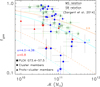 |
Fig. 14. Gas fraction fgas = Mgas/(Mgas + ℳ) as a function of ℳ. The symbols are defined as in Fig. 13. The solid and dashed curves represent the expected relations for MS and SB galaxies, respectively, at z = 1.5 (cyan) and at z = 2.5 (orange). |
To further investigate this mass dependency and take into account each source offset from the MS, we analyse MS-normalised quantities (see Sargent et al. 2014; Genzel et al. 2015; Scoville et al. 2016; Tacconi et al. 2018). In particular, we show in Fig. 15 the normalised gas fraction, defined as μmol/⟨μmol⟩MS, where μmol ≡ Mmol/ℳ, and the offset from the MS in terms of starburstiness, that is SFR/⟨SFRMS⟩, for our ALMA sources and for cluster and proto-cluster galaxies from the literature, and compare them with the values predicted by the “2-Star Formation Mode” (2-SFM) framework formulated by Sargent et al. (2014). The 2-SFM predicted values are independent of stellar mass and redshift and take into account the type (MS or SB) of source that dominates as a function of starburstiness. The 2-SFM framework assumes a continuous distribution of αCO conversion factors that varies according to the position of a source in the SFR-ℳ diagram, rather than two distinct values for MS and SB galaxies. The diagram in Fig. 15 confirms that most MS galaxies with ℳ > 1011 M⊙ (shown as magenta squares) have gas fractions below the expected values (i.e. only one out of eight sources with ℳ> 1011 M⊙ is above the relation, while five are below). The same is not true among SB galaxies. ISM mass fractions are also systematically lower for the ALMA sources with ℳ> 1011 M⊙, although still consistent with the 2-SFM relation. However, we caution the use of mm-continuum ISM masses as proxies for CO molecular gas masses as they might be affected by systematic uncertainties. For example, in the two cases of our sample for which CO masses are available, ISM masses are higher than the CO masses, possibly suggesting that the ISM-derived masses are overestimates. Keeping this caveat in mind, we conclude that gas fractions based on ISM masses tend to be lower for galaxies with ℳ > 1011 M⊙. Our analysis also indicates a notable difference, both in excess (for cluster and proto-cluster members), and in deficiency (only for cluster galaxies), between measured and predicted gas fractions. The observed wide range of gas fractions may suggest that in dense environments these change quickly, or at least faster than their SFRs.
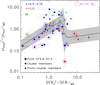 |
Fig. 15. Normalised molecular gas mass fraction μmol ≡ Mgas/ℳ as a function of the normalised SFR. The symbols are defined as in Fig. 13. The black solid curve and grey area represent the values predicted by the 2-SFM framework described in Sargent et al. (2014). Sources with ℳ > 1011 M⊙ are shown with magenta large squares. The grey area shows the expected 1σ scatter around the average molecular gas mass fraction. |
We note that this analysis is not aimed at obtaining a comprehensive picture of SFEs and gas fractions in field, cluster, and proto-cluster galaxies, but is instead simply aimed at comparing our ALMA sources to what is available in the literature (keeping in mind that those samples are often biased towards the most gas-rich members). To limit this bias, we also include data from two clusters for which a large number of members with deep CO data are available (Rudnick et al. 2017; Hayashi et al. 2017) in the SFE analysis; however, stellar masses are not available for the latter, so they are missing in our gas-fraction analysis. A future analysis of the gas fraction in an unbiased sample of 1 < z < 3 galaxies in clusters and proto-clusters could reveal the processes and the timescales that affect the cold gas as a function of environment.
7. Discussion
We have found that the ALMA-detected galaxies comprising this Planck peak are primarily main-sequence galaxies that break-up into redshift groups, with the galaxies associated with individual Herschel flux regions not necessarily falling into the same redshift ranges.
In ALMA fields 5 and 8 only a single ALMA galaxy is observed, and these are thus simple to interpret. In both cases the fluxes are attributed to a low redshift galaxy (z ≲ 1.3). The other ALMA fields contain multiple sources and in most of the cases they are at different redshifts. The only exceptions are IDs 5 and 6 in field 3, and IDs 13, 14, and 15 in field 7. The tentative picture that emerges puts ALMA fields 1, 5 and 8 at z ≃ 1, ALMA fields 2, 3, 4, and 6 at z ≃ 1.5, and ALMA fields 1, 6, and 7 at z ≃ 2.4. But reality may not be quite so simple, as evidenced by the various “interlopers” found in several of the fields, which seem to indicate that some regions cannot really be categorised as belonging to one group or the other, but contain mixtures of high and low redshift galaxies. Broadly speaking, however, the nature of G073.4−57.5 seems to be at least two line-of-sight structures at z ≃ 1.5 and z ≃ 2.4, and probably a few other galaxies at different redshifts. This conclusion seems reasonable, since G073.4−57.5 appears similar to the Planck peak G95.5−61.6 (Flores-Cacho et al. 2016), in the sense that it is a superposition of two independent structures on the sky (in the case of G95.5−61.6, the two groups are at z = 1.7 and z = 2.0). It also ties in with the simulation results of Negrello et al. (2017), who found that the number of Planck peaks exceeds the number of single massive haloes expected at redshifts z = 1.5–3, and that the majority of Planck peaks are consistent with being superpositions of proto-clusters.
We have also investigated our photometric redshift distribution in the context of the sky simulation catalogue of Béthermin et al. (2017). First, using the whole catalogue, the expected number of detections in 1.8 arcmin2 is 2.9 sources, broadly consistent with the average source counts we adopt from the literature, and giving a 6-times higher observed source density. It is beyond the scope of this paper to attempt a modelling of all the selection effects that enter into the final detection with ALMA, or a detailed comparison of the clustering we find within the photometric redshift distribution; however, one thing we can easily do is compare the simulated redshift distribution for all sources, renormalised to the observed number of sources (and in coarse redshift bins of Δz = 0.85) with the observed distribution. We find that we see no significant difference, given the relatively large Poisson errors (the Kolmogorov–Smirnov p-value is 0.22); in the z = 0.85–1.7 redshift bin 3.0 more sources are observed than expected in the renormalised distribution (9.9 times higher than the simulated numbers) and in the z = 1.7–2.55 redshift bin 1.6 more sources are observed than expected when renormalised (8.0 times higher compared to simulated numbers).
Going back to the Spitzer and CFHT colour-magnitude and colour-colour diagrams (Figs. 4 and 5), we see that four out of five member candidates at z ≃ 1.5 (i.e. ALMA IDs 3, 5, 6, and 8) exhibit similar J − Ks and [3.6] − [4.5] colours, in good agreement with the photo-z results and our interpretation. The other z ≃ 1.5 member candidate, ID 12, shows consistency only in the IRAC colour, but not in the NIR colour. Similarly, ALMA IDs 1, 11, 13, and 15, member candidates in the z ≃ 2.4 structure, show similar IRAC and NIR colours (the latter is not available for ID 1). The other member candidate, ID 14, was not included in the colour analysis because it is undetected in the NIR.
The SED-fitting procedure used in this paper is based on an unusual set of filters that combine four wavelengths in the NIR (1–5 μm) and five in the FIR-mm (250–1300 μm). Most high-z dusty galaxies (and obscured AGN) are characterised by red NIR colours, thus the redshift is mostly constrained by the peak location of the FIR component. In five cases the stellar peak is clearly visible in the NIR SED (IDs 0, 4, 10, 16, and 17) and the resulting redshift is below 1.3, and in all other cases the stellar peak is redshifted to λ > 4.5 μm, or alternatively an AGN might be present. Because of the lack of mid-IR data, the presence of an AGN cannot be easily determined, and thus it cannot be completely ruled out. Our best fits suggest that two sources are AGN, and each of them is associated with one of the two structures: ID 6 with the structure at z = 1.5; and ID 15 with that at z = 2.4. In high-z proto-clusters, accretion onto a supermassive black hole is expected to be favoured with respect to the field because of the presence of cold gas, high galaxy density, and modest relative velocities. Previous work targeted at quantifying the AGN fraction in proto-clusters yields conflicting results (e.g. Krishnan et al. 2017; Lehmer et al. 2013; Digby-North et al. 2010; Macuga et al. 2019). Our results, based on the SED fits, indicate that one out of five (20 ± 9%) members of each structure is an AGN. Although this fraction is consistent with the findings in other high-z structures (i.e. 17%, Lehmer et al. 2013; Krishnan et al. 2017), our result is only suggestive. In order to quantify its significance we would firstly need to confirm the membership of each structure, and, secondly quantify the AGN fraction in the field by applying the same technique.
While our work is carried out in the context of searching for “proto-clusters”, that is early structures that are not yet virialised, with our findings of two overdensities of mm galaxies we cannot be sure if either is in fact already a “cluster”. We have no information about the thermal state of any intra-cluster medium, since the limits available from the X-ray ROSAT all-sky survey and the Planck Sunyaev–Zeldovich cluster survey are too weak; our overdensities should perhaps be identified simply as “structures”.
The two possible structures revealed by our selection in the mm range at z ≃ 1.5 and 2.4 have members distributed over six ALMA fields. Those at z ≃ 1.5 are distributed over a narrow region 4′ long (5.2 comoving Mpc at z = 1.5), connecting fields 2, 3, 4, and 6. The member candidates of the z ≃ 2.4 structure are distributed over fields 1, 6, and 7, corresponding to a region of about 2′ × 2′ (3.4 Mpc × 3.4 Mpc comoving at z = 2.4). The total SFRs of the two structures at z = 1.5, and 2.4 are 840 yr−1 and 1020
 yr−1, respectively; the total stellar masses are 5.8
 and 4.2
 , respectively. The members in the lower-z structure are all quite massive and located on the MS. Those in the higher-z structure are instead a mix of massive and more typical sources that are, respectively, on the MS or above. These results are based on photometric redshifts with considerable uncertainty, but if confirmed they would indicate that the members in the low-z structure are mature and close to the end of their active growth, while some of those in the high-z structure are still active (SB-like) and growing. The analysis of SFEs and gas fractions, possible for only two galaxies, IDs 3 and 8, both in the z = 1.5 structure, yield values consistent with the MS relation for ID 3 and inconsistent with either the MS or SB relations for ID 8. The CO luminosity in the latter source is anomalously low, casting some doubts on its association with the observed continuum. The gas fractions of our ALMA sources, based on the dust continuum, combined with those from the literature, indicate that proto-cluster members are more gas-rich than the isolated field (MS or SB) galaxies for ℳ < 1011 M⊙; the gas fractions drops by almost a factor of two at larger stellar masses.
The lack of strong CO lines for the other sources at z ≃1.5 might imply that their molecular gas is depleted. On the other hand, it is possible that we did not detect lines from any other galaxies because they lie outside of our observed spectral window. Indeed, the line of ALMA ID 3 clearly extends beyond the high frequency end of the spectral window.
It is a valid question to ask whether gravitational galaxy-galaxy lensing can play a role in enhancing the counts in a scenario where extended structures at lower and higher redshift overlap along the line of sight, giving apparent densities above typical proto-cluster measurements. In the current data most ALMA sources are positionally well matched with Spitzer and NIR data and contain no indication of lensing signatures, while only a few sources show offsets (as seen in Fig. 3) between the mm and NIR emission (e.g. ALMA IDs 1, 4, and 15). In terms of statistical arguments, in general the probability for strong galaxy-galaxy lensing is small; for example, van der Wel et al. (2013) estimate one source per 200 arcmin2 for average counts of strongly lensed sources. However, lensing cannot be completely ruled out, and in particular smaller flux boosts by factors less than 2 could be common, since in our case the counts are enhanced (possibly by a factor of 10 for both the source and the lensed population), and the region was selected for high submm surface brightness in the first place.
8. Conclusions
Using ALMA in only 24 min of on-source time we find 18 individual mm galaxies, showing that follow-up of the Planck high-z sample through targeted pointings of Herschel-SPIRE sources is an efficient use of this telescope. For the first time we are directly resolving the Planck peaks and the Herschel-SPIRE overdensities into individual galaxies at mm wavelengths. The ALMA detections are well matched with Spitzer-IRAC sources in all but one case and mostly show excellent positional agreement (typically < 0.4″); three sources that are offset by up to 1″ are extended in Spitzer, and may either be blended or have intrinsically more complex structure.
The surface density of the mm galaxies within the ALMA pointings is 8–30 times higher than the average counts, and we estimate an SFR of ≃ 2700 M⊙ yr−1 (of which one third can be attributed to sources consistent with z ≃ 1.5 and another third to sources at z ≃ 2.4). Furthermore, the SCUBA-2 data indicate that we have not recovered all of the mm galaxies in this field, possibly not even the brightest, which will require a wider mosaic. Nevertheless, we can conclude that the Planck peak G073.4−57.5 consists of a large number of moderately bright mm galaxies, rather than a few extremely bright galaxies. Typical proto-clusters (such as the COSMOS z = 2.47 structure or the SSA22 z = 3.09 structure) contain fewer galaxies than we have detected, perhaps because G073.4−57.5 is a line-of-sight superposition of two massive structures. The cluster XCS J2215.9−1738 at z = 1.46 also shows a high density of ALMA galaxies, but those are fainter.
NIR colour diagrams of the ALMA-detected galaxies reveal a “red sequence”, a characteristic feature of z > 1.3 structures that are the progenitors of later massive galaxy clusters. An NIR+FIR photo-z analysis indicates a concentration at z ≃ 1.5, while a second structure at higher redshift (z ≃ 2.4) could be present as well, consistent with the interpretation of two line-of-sight structures. In addition to photometric redshifts, we present SFRs, IR luminosities, stellar masses, dust temperatures, dust masses, and gas masses for these galaxies. Three galaxies can clearly be identified as starbursts (i.e. lying a factor of 3 or more above the MS), ID 8 at z ≃ 1.5 and IDs 1 and 14 at z ≃ 2.4, while most of the galaxies are within the normal range of SFRs for their stellar masses.
Serendipitous line detections of two galaxies at a common frequency (ΔV< 300 km s−1) are interpreted as the CO(5–4) transition and can be used to fix the redshift of the main structure to z = 1.5434 ± 0.0010, in agreement with the photo-z estimates. However, this needs to be confirmed with additional spectroscopy.
The CO luminosity of ID 3, combined with the parameters derived from the SED fitting, indicate that the molecular gas in this source is similar to a normal star-forming galaxy, but with a smaller SFE, as well as a larger gas mass and fraction than expected based on the MS relation. The CO properties of ID 8 are instead inconsistent with the relations observed for MS or SB galaxies. Based on the SFR–ℳ relation, ID 8 is an SB galaxy with a modest offset from the MS, but its SFE and gas mass are, respectively, unusually high and low with respect to expectations for isolated field galaxies. Interestingly, its ISM mass is much higher than the CO-derived mass, bringing both its SFE and gas fraction into agreement with the expectation.
The overall analysis of stellar masses, SFRs, and gas fractions of the ALMA sources in the two structures at z = 1.5 and 2.4 suggest that the former contains more evolved galaxies with stellar masses larger than the expected ℳ*, and SFRs consistent with the MS, while the latter contains a mix of sources, some more massive than the expected ℳ*, and with moderate to low SFRs, or with stellar masses consistent with the expected ℳ*, but with SFRs above the MS and in the SB region. These results, derived from a mm/submm selection and to be confirmed with more accurate redshifts, are consistent with a scenario in which the structure at lower redshift is more mature and most of its members have reached the end of their active phase; however, the structure at higher redshift contains some galaxies that are instead still actively growing.
The analysis of the cold gas properties (traced by CO emission or by the mm continuum) for our ALMA detections and for galaxies in clusters and proto-clusters at 1 < z < 3, have revealed two interesting results. Firstly, cluster and proto-cluster galaxies with stellar masses < 1011 M⊙ exhibit a broad range of gas fractions, suggesting that the gas content can change quickly in dense environments. Secondly, most cluster and proto-cluster galaxies with stellar masses > 1011 M⊙ are gas deficient with respect to field galaxies. These results are valid only for normal SFGs, and not for SB galaxies, but this should be confirmed with unbiased CO samples.
There are several important aspects of our study that should be followed up. First, optical/NIR or mm spectroscopy (see e.g. Casey et al. 2017) will allow us to confirm the photo-z estimates and the associations of the individual galaxies with structures in redshift space. Second, it will be helpful to associate all SCUBA-2 sources with their counterparts in ALMA data in order to study those brightest submm peaks in more detail. Third, it is important to address the positional offsets between the NIR and FIR images with future high-resolution data, in particular by searching for elongations or multiple images that would be evidence of strong lensing. And lastly, further imaging and spectroscopy of this Planck peak will enable us to characterise its physical properties in terms of angular and redshift-space morphology and to build a census of its stellar and star-forming properties. Such a detailed study is the only way to determine the nature of these red peaks in the CIB that have been picked out by Planck, which is the most decisive step in determining what exactly they are teaching us about structure formation.
We note that for the latest Planck release (Planck Collaboration Int. XXXIX 2016), G073.4−57.5 lies just inside the more conservatively applied Galactic mask.
While we show here that a physically motivated approach exists, we stress that we use the resulting equation in a phenomenological sense, that is with a single normalisation factor per source.
 .
.
The relationship assumed here for MS galaxies is the following:
![Mathematical equation: $$ \begin{aligned} \log (\mathrm{SFR}_{\rm MS})=&\left[\,(0.84\pm 0.02) - (0.026\pm 0.003) \times t(z)\,\right] \times \log (\mathcal{M} )\nonumber \\&-\left[\,(6.51\pm 0.24) - (0.11\pm 0.03) \times t(z)\,\right], \end{aligned} $$](/articles/aa/full_html/2019/05/aa33252-18/aa33252-18-eq216.gif) (4)
(4)
where t(z) is the age of the Universe in Gyr at redshift z, ℳ is the stellar mass in M⊙, and SFRMS is the star-formation rate in M⊙ yr−1.
The predicted CO(1–0) line luminosity scales with to the total IR luminosity as:
 (5)
(5)
for MS galaxies, while for SB galaxies
 (6)
(6)
with LIR in L⊙, and  in K km s−1 pc2.
For ID 3, we estimate MISM = (3.0 ± 0.2) 1011 M⊙, and Mmol = (2.0 ± 0.4) 1011 M⊙, thus the difference between MISM and Mmol for ID 3 is (1.0 ± 0.5) 1011 M⊙.
Acknowledgments
We thank the referee for valuable suggestions that improved the paper. MP acknowledges financial support from Labex OCEVU, CM acknowledges the support provided by FONDECYT postdoctoral research grant no. 3170774, and RH and DS acknowledge support from the Natural Sciences and Engineering Research Council of Canada. This work has been carried out thanks to the support of the OCEVU Labex (ANR-11-LABX-0060) and the A*MIDEX project (ANR-11-IDEX-0001-02) funded by the “Investissements d’Avenir” French government programme managed by the ANR. This work is mainly based on the following ALMA data: ADS/JAO.ALMA# 2013.1.01173.S. ALMA is a partnership of ESO (representing its member states), NSF (USA), and NINS (Japan), together with NRC (Canada), NSC, and ASIAA (Taiwan), and KASI (Republic of Korea), in cooperation with the Republic of Chile. The Joint ALMA Observatory is operated by ESO, AUI/NRAO, and NAOJ. The development of Planck has been supported by: ESA; CNES and CNRS/INSU-IN2P3-INP (France); ASI, CNR, and INAF (Italy); NASA and DoE (USA); STFC and UKSA (UK); CSIC, MICINN, JA, and RES (Spain); Tekes, AoF, and CSC (Finland); DLR and MPG (Germany); CSA (Canada); DTU Space (Denmark); SER/SSO (Switzerland);RCN (Norway); SFI (Ireland); FCT/MCTES (Portugal); and PRACE (EU). Herschel is an ESA space observatory with science instruments provided by European-led Principal Investigator consortia and with important participation from NASA. This work is based in part on observations made with the Spitzer Space Telescope, which is operated by the Jet Propulsion Laboratory, California Institute of Technology under a contract with NASA. This research has made use of the NASA/ IPAC Infrared Science Archive, which is operated by the Jet Propulsion Laboratory, California Institute of Technology, under contract with the National Aeronautics and Space Administration. This publication makes use of data products from the Wide-field Infrared Survey Explorer, which is a joint project of the University of California, Los Angeles, and the Jet Propulsion Laboratory/California Institute of Technology, and NEOWISE, which is a project of the Jet Propulsion Laboratory/California Institute of Technology; WISE and NEOWISE are funded by the National Aeronautics and Space Administration. The James Clerk Maxwell Telescope has historically been operated by the Joint Astronomy Centre on behalf of the Science and Technology Facilities Council of the United Kingdom, the National Research Council of Canada, and the Netherlands Organisation for Scientific Research. Additional funds for the construction of SCUBA-2 were provided by the Canada Foundation for Innovation. The Pan-STARRS1 Surveys (PS1) and the PS1 public science archive have been made possible through contributions by the Institute for Astronomy, the University of Hawaii, the Pan-STARRS Project Office, the Max-Planck Society and its participating institutes, the Max Planck Institute for Astronomy, Heidelberg and the Max Planck Institute for Extraterrestrial Physics, Garching, The Johns Hopkins University, Durham University, the University of Edinburgh, the Queen’s University Belfast, the Harvard-Smithsonian Center for Astrophysics, the Las Cumbres Observatory Global Telescope Network Incorporated, the National Central University of Taiwan, the Space Telescope Science Institute, the National Aeronautics and Space Administration under Grant No. NNX08AR22G issued through the Planetary Science Division of the NASA Science Mission Directorate, the National Science Foundation Grant No. AST-1238877, the University of Maryland, Eotvos Lorand University (ELTE), the Los Alamos National Laboratory, and the Gordon and Betty Moore Foundation.
References
- Aravena, M., Carilli, C. L., Salvato, M., et al. 2012, MNRAS, 426, 258 [NASA ADS] [CrossRef] [Google Scholar]
- Barro, G., Pérez-González, P. G., Gallego, J., et al. 2011, ApJS, 193, 30 [NASA ADS] [CrossRef] [Google Scholar]
- Becker, R. H., White, R. L., & Helfand, D. J. 1995, ApJ, 450, 559 [NASA ADS] [CrossRef] [Google Scholar]
- Bertin, E., & Arnouts, S. 1996, A&AS, 117, 393 [NASA ADS] [CrossRef] [EDP Sciences] [Google Scholar]
- Béthermin, M., Wu, H.-Y., Lagache, G., et al. 2017, A&A, 607, A89 [NASA ADS] [CrossRef] [EDP Sciences] [Google Scholar]
- Blain, A. W., & Longair, M. S. 1993, MNRAS, 264, 509 [NASA ADS] [CrossRef] [Google Scholar]
- Blain, A. W., Chapman, S. C., Smail, I., & Ivison, R. 2004, ApJ, 611, 725 [NASA ADS] [CrossRef] [Google Scholar]
- Bolatto, A. D., Wolfire, M., & Leroy, A. K. 2013, ARA&A, 51, 207 [Google Scholar]
- Bolzonella, M., Miralles, J.-M., & Pelló, R. 2000, A&A, 363, 476 [NASA ADS] [Google Scholar]
- Bothwell, M. S., Smail, I., Chapman, S. C., et al. 2013, MNRAS, 429, 3047 [NASA ADS] [CrossRef] [Google Scholar]
- Brammer, G. B., van Dokkum, P. G., & Coppi, P. 2008, ApJ, 686, 1503 [NASA ADS] [CrossRef] [Google Scholar]
- Bruzual, G., & Charlot, S. 2003, MNRAS, 344, 1000 [NASA ADS] [CrossRef] [Google Scholar]
- Cañameras, R., Nesvadba, N. P. H., Guery, D., et al. 2015, A&A, 581, A105 [NASA ADS] [CrossRef] [EDP Sciences] [Google Scholar]
- Cañameras, R., Nesvadba, N., Kneissl, R., et al. 2017a, A&A, 604, A117 [NASA ADS] [CrossRef] [EDP Sciences] [Google Scholar]
- Cañameras, R., Nesvadba, N. P. H., Kneissl, R., et al. 2017b, A&A, 600, L3 [NASA ADS] [CrossRef] [EDP Sciences] [Google Scholar]
- Cañameras, R., Yang, C., Nesvadba, N. P. H., et al. 2018a, A&A, 620, A61 [NASA ADS] [CrossRef] [EDP Sciences] [Google Scholar]
- Cañameras, R., Nesvadba, N. P. H., Limousin, M., et al. 2018b, A&A, 620, A60 [NASA ADS] [CrossRef] [EDP Sciences] [Google Scholar]
- Capak, P. L., Riechers, D., Scoville, N. Z., et al. 2011, Nature, 470, 233 [Google Scholar]
- Carilli, C. L., & Walter, F. 2013, ARA&A, 51, 105 [NASA ADS] [CrossRef] [EDP Sciences] [Google Scholar]
- Carniani, S., Maiolino, R., De Zotti, G., et al. 2015, A&A, 584, A78 [NASA ADS] [CrossRef] [EDP Sciences] [Google Scholar]
- Carter, M., Lazareff, B., Maier, D., et al. 2012, A&A, 538, A89 [NASA ADS] [CrossRef] [EDP Sciences] [Google Scholar]
- Casasola, V., Magrini, L., Combes, F., et al. 2013, A&A, 558, A60 [NASA ADS] [CrossRef] [EDP Sciences] [Google Scholar]
- Casey, C. M. 2012, MNRAS, 425, 3094 [Google Scholar]
- Casey, C. M. 2016, ApJ, 824, 36 [NASA ADS] [CrossRef] [EDP Sciences] [Google Scholar]
- Casey, C. M., Chen, C.-C., Cowie, L. L., et al. 2013, MNRAS, 436, 1919 [NASA ADS] [CrossRef] [Google Scholar]
- Casey, C. M., Cooray, A., Capak, P., et al. 2015, ApJ, 808, L33 [NASA ADS] [CrossRef] [Google Scholar]
- Casey, C. M., Cooray, A., Killi, M., et al. 2017, ApJ, 840, 101 [NASA ADS] [CrossRef] [Google Scholar]
- Castignani, G., Combes, F., Salomé, P., et al. 2018, A&A, 617, A103 [NASA ADS] [CrossRef] [EDP Sciences] [Google Scholar]
- Castignani, G., Combes, F., Salomé, P., et al. 2019, A&A, 623, A48 [NASA ADS] [CrossRef] [EDP Sciences] [Google Scholar]
- Chabrier, G. 2003, PASP, 115, 763 [NASA ADS] [CrossRef] [Google Scholar]
- Chambers, K. C., Magnier, E. A., Metcalfe, N., et al. 2019, ArXiv e-prints [arXiv:1612.05560v4] [Google Scholar]
- Chapman, S. C., Lewis, G. F., Scott, D., et al. 2001, ApJ, 548, L17 [NASA ADS] [CrossRef] [Google Scholar]
- Clements, D. L., Dunne, L., & Eales, S. 2010, MNRAS, 403, 274 [NASA ADS] [CrossRef] [Google Scholar]
- Clements, D. L., Braglia, F. G., Hyde, A. K., et al. 2014, MNRAS, 439, 1193 [NASA ADS] [CrossRef] [Google Scholar]
- Clements, D. L., Braglia, F., Petitpas, G., et al. 2016, MNRAS, 461, 1719 [NASA ADS] [CrossRef] [Google Scholar]
- Coogan, R. T., Daddi, E., Sargent, M. T., et al. 2018, MNRAS, 479, 703 [NASA ADS] [Google Scholar]
- Daddi, E., Dannerbauer, H., Liu, D., et al. 2015, A&A, 577, A46 [NASA ADS] [CrossRef] [EDP Sciences] [Google Scholar]
- Dale, D. A., Aniano, G., Engelbracht, C. W., et al. 2012, ApJ, 745, 95 [NASA ADS] [CrossRef] [Google Scholar]
- Danielson, A. L. R., Swinbank, A. M., Smail, I., et al. 2017, ApJ, 840, 78 [NASA ADS] [CrossRef] [Google Scholar]
- Dannerbauer, H., Lehnert, M. D., Emonts, B., et al. 2017, A&A, 608, A48 [NASA ADS] [CrossRef] [EDP Sciences] [Google Scholar]
- Davidzon, I., Ilbert, O., Laigle, C., et al. 2017, A&A, 605, A70 [NASA ADS] [CrossRef] [EDP Sciences] [Google Scholar]
- Digby-North, J. A., Nandra, K., Laird, E. S., et al. 2010, MNRAS, 407, 846 [NASA ADS] [CrossRef] [Google Scholar]
- Draine, B. T. 2011, Physics of the Interstellar and Intergalactic Medium (Princeton: Princeton University Press) [Google Scholar]
- Dunlop, J. S., McLure, R. J., Biggs, A. D., et al. 2017, MNRAS, 466, 861 [NASA ADS] [CrossRef] [Google Scholar]
- Elbaz, D., Dickinson, M., Hwang, H. S., et al. 2011, A&A, 533, A119 [NASA ADS] [CrossRef] [EDP Sciences] [Google Scholar]
- Flores-Cacho, I., Pierini, D., Soucail, G., et al. 2016, A&A, 585, A54 [NASA ADS] [CrossRef] [EDP Sciences] [Google Scholar]
- Foltz, R., Wilson, G., Muzzin, A., et al. 2018, ApJ, 866, 136 [NASA ADS] [CrossRef] [Google Scholar]
- Franx, M., Labbé, I., Rudnick, G., et al. 2003, ApJ, 587, L79 [NASA ADS] [CrossRef] [Google Scholar]
- Fujimoto, S., Ouchi, M., Ono, Y., et al. 2016, ApJS, 222, 1 [NASA ADS] [CrossRef] [Google Scholar]
- Genzel, R., Tacconi, L. J., Lutz, D., et al. 2015, ApJ, 800, 20 [NASA ADS] [CrossRef] [Google Scholar]
- Gildas Team 2013, Astrophysics Source Code Library [record ascl:1305.010] [Google Scholar]
- González-López, J., Bauer, F. E., Romero-Cañizales, C., et al. 2016, A&A, 597, A41 [Google Scholar]
- Greenslade, J., Clements, D. L., Cheng, T., et al. 2018, MNRAS, 476, 3336 [NASA ADS] [CrossRef] [Google Scholar]
- Guiderdoni, B., Bouchet, F. R., Puget, J.-L., Lagache, G., & Hivon, E. 1997, Nature, 390, 257 [NASA ADS] [CrossRef] [Google Scholar]
- Hatch, N. A., Muldrew, S. I., Cooke, E. A., et al. 2016, MNRAS, 459, 387 [NASA ADS] [CrossRef] [Google Scholar]
- Hatsukade, B., Ohta, K., Seko, A., Yabe, K., & Akiyama, M. 2013, ApJ, 769, L27 [NASA ADS] [CrossRef] [Google Scholar]
- Hatsukade, B., Kohno, K., Umehata, H., et al. 2016, PASJ, 68, 36 [NASA ADS] [CrossRef] [Google Scholar]
- Hayashi, M., Kodama, T., Tadaki, K.-I., Koyama, Y., & Tanaka, I. 2012, ApJ, 757, 15 [NASA ADS] [CrossRef] [Google Scholar]
- Hayashi, M., Kodama, T., Kohno, K., et al. 2017, ApJ, 841, L21 [NASA ADS] [CrossRef] [Google Scholar]
- Herranz, D., González-Nuevo, J., Clements, D. L., et al. 2013, A&A, 549, A31 [NASA ADS] [CrossRef] [EDP Sciences] [Google Scholar]
- Hildebrand, R. H. 1983, QJRAS, 24, 267 [NASA ADS] [Google Scholar]
- Ivison, R. J., Magnelli, B., Ibar, E., et al. 2010, A&A, 518, L31 [NASA ADS] [CrossRef] [EDP Sciences] [Google Scholar]
- Ivison, R. J., Swinbank, A. M., Smail, I., et al. 2013, ApJ, 772, 137 [NASA ADS] [CrossRef] [Google Scholar]
- Kannappan, S. J., & Gawiser, E. 2007, ApJ, 657, L5 [NASA ADS] [CrossRef] [Google Scholar]
- Kennicutt, Jr., R. C. 1998, ARA&A, 36, 189 [Google Scholar]
- Krishnan, C., Hatch, N. A., Almaini, O., et al. 2017, MNRAS, 470, 2170 [NASA ADS] [CrossRef] [Google Scholar]
- Lacy, M., Wilson, G., Masci, F., et al. 2005, ApJS, 161, 41 [NASA ADS] [CrossRef] [Google Scholar]
- Lee, M. M., Tanaka, I., Kawabe, R., et al. 2017, ApJ, 842, 55 [CrossRef] [Google Scholar]
- Lehmer, B. D., Lucy, A. B., Alexander, D. M., et al. 2013, ApJ, 765, 87 [NASA ADS] [CrossRef] [Google Scholar]
- Lilly, S. J., Eales, S. A., Gear, W. K. P., et al. 1999, ApJ, 518, 641 [NASA ADS] [CrossRef] [Google Scholar]
- MacKenzie, T. P., Scott, D., Bianconi, M., et al. 2017, MNRAS, 468, 4006 [NASA ADS] [CrossRef] [Google Scholar]
- Macuga, M., Martini, P., Miller, E. D., et al. 2019, ApJ, 874, 54 [NASA ADS] [CrossRef] [Google Scholar]
- Magnelli, B., Lutz, D., Saintonge, A., et al. 2014, A&A, 561, A86 [NASA ADS] [CrossRef] [EDP Sciences] [Google Scholar]
- Mainzer, A., Bauer, J., Grav, T., et al. 2011, ApJ, 731, 53 [NASA ADS] [CrossRef] [Google Scholar]
- Martinache, C., Rettura, A., Dole, H., et al. 2018, A&A, 620, A198 [NASA ADS] [CrossRef] [EDP Sciences] [Google Scholar]
- McMullin, J. P., Waters, B., Schiebel, D., Young, W., & Golap, K. 2007, in Astronomical Data Analysis Software and Systems XVI, eds. R. A. Shaw, F. Hill, & D. J. Bell, ASP Conf. Ser., 376, 127 [Google Scholar]
- Muñoz Arancibia, A. M., González-López, J., Ibar, E., et al. 2018, A&A, 620, A125 [NASA ADS] [CrossRef] [EDP Sciences] [Google Scholar]
- Muzzin, A., Marchesini, D., Stefanon, M., et al. 2013, ApJ, 777, 18 [NASA ADS] [CrossRef] [Google Scholar]
- Narayanan, D., Turk, M., Feldmann, R., et al. 2015, Nature, 525, 496 [NASA ADS] [CrossRef] [PubMed] [Google Scholar]
- Negrello, M., Gonzalez-Nuevo, J., De Zotti, G., et al. 2017, MNRAS, 470, 2253 [NASA ADS] [CrossRef] [Google Scholar]
- Nesvadba, N., Kneissl, R., Cañameras, R., et al. 2016, A&A, 593, L2 [NASA ADS] [CrossRef] [EDP Sciences] [Google Scholar]
- Nesvadba, N., Canameras, R., Kneissl, R., et al. 2019, A&A, 624, A23 [NASA ADS] [CrossRef] [EDP Sciences] [Google Scholar]
- Nguyen, H. T., Schulz, B., Levenson, L., et al. 2010, A&A, 518, L5 [NASA ADS] [CrossRef] [EDP Sciences] [Google Scholar]
- Noble, A. G., McDonald, M., Muzzin, A., et al. 2017, ApJ, 842, L21 [Google Scholar]
- Ono, Y., Ouchi, M., Kurono, Y., & Momose, R. 2014, ApJ, 795, 5 [NASA ADS] [CrossRef] [Google Scholar]
- Oteo, I., Zwaan, M. A., Ivison, R. J., Smail, I., & Biggs, A. D. 2016, ApJ, 822, 36 [NASA ADS] [CrossRef] [Google Scholar]
- Oteo, I., Ivison, R. J., Dunne, L., et al. 2018, ApJ, 856, 72 [Google Scholar]
- Overzier, R. A. 2016, A&ARv, 24, 14 [NASA ADS] [CrossRef] [Google Scholar]
- Papovich, C. 2008, ApJ, 676, 206 [NASA ADS] [CrossRef] [Google Scholar]
- Perna, M., Sargent, M. T., Brusa, M., et al. 2018, A&A, 619, A90 [NASA ADS] [CrossRef] [EDP Sciences] [Google Scholar]
- Pilbratt, G. L., Riedinger, J. R., Passvogel, T., et al. 2010, A&A, 518, L1 [CrossRef] [EDP Sciences] [Google Scholar]
- Planck Collaboration XXI. 2011, A&A, 536, A21 [NASA ADS] [CrossRef] [EDP Sciences] [Google Scholar]
- Planck Collaboration I. 2014, A&A, 571, A1 [NASA ADS] [CrossRef] [EDP Sciences] [Google Scholar]
- Planck Collaboration XVIII. 2014, A&A, 571, A18 [NASA ADS] [CrossRef] [EDP Sciences] [Google Scholar]
- Planck Collaboration XXVII. 2016, A&A, 594, A27 [NASA ADS] [CrossRef] [EDP Sciences] [Google Scholar]
- Planck Collaboration VI. 2018, A&A, submitted [arXiv:1807.06209] [Google Scholar]
- Planck Collaboration Int. XXVII. 2015, A&A, 582, A30 [NASA ADS] [CrossRef] [EDP Sciences] [Google Scholar]
- Planck Collaboration Int. XXXIX. 2016, A&A, 596, A100 [NASA ADS] [CrossRef] [EDP Sciences] [Google Scholar]
- Pokhrel, R., Gutermuth, R., Ali, B., et al. 2016, MNRAS, 461, 22 [NASA ADS] [CrossRef] [PubMed] [Google Scholar]
- Polletta, M., Tajer, M., Maraschi, L., et al. 2007, ApJ, 663, 81 [NASA ADS] [CrossRef] [Google Scholar]
- Popping, G., Somerville, R. S., & Galametz, M. 2017, MNRAS, 471, 3152 [NASA ADS] [CrossRef] [Google Scholar]
- Rémy-Ruyer, A., Madden, S. C., Galliano, F., et al. 2014, A&A, 563, A31 [NASA ADS] [CrossRef] [EDP Sciences] [Google Scholar]
- Rettura, A., Martinez-Manso, J., Stern, D., et al. 2014, ApJ, 797, 109 [NASA ADS] [CrossRef] [Google Scholar]
- Rodighiero, G., Daddi, E., Baronchelli, I., et al. 2011, ApJ, 739, L40 [NASA ADS] [CrossRef] [Google Scholar]
- Rudnick, G., Hodge, J., Walter, F., et al. 2017, ApJ, 849, 27 [NASA ADS] [CrossRef] [Google Scholar]
- Sanders, D. B., Soifer, B. T., Elias, J. H., et al. 1988, ApJ, 325, 74 [NASA ADS] [CrossRef] [Google Scholar]
- Sargent, M. T., Daddi, E., Béthermin, M., et al. 2014, ApJ, 793, 19 [NASA ADS] [CrossRef] [Google Scholar]
- Sawicki, M. 2002, AJ, 124, 3050 [NASA ADS] [CrossRef] [Google Scholar]
- Scoville, N., Aussel, H., Sheth, K., et al. 2014, ApJ, 783, 84 [NASA ADS] [CrossRef] [Google Scholar]
- Scoville, N., Sheth, K., Aussel, H., et al. 2016, ApJ, 820, 83 [NASA ADS] [CrossRef] [Google Scholar]
- Socolovsky, M., Almaini, O., Hatch, N. A., et al. 2018, MNRAS, 476, 1242 [NASA ADS] [CrossRef] [Google Scholar]
- Solomon, P. M., Downes, D., Radford, S. J. E., & Barrett, J. W. 1997, ApJ, 478, 144 [NASA ADS] [CrossRef] [Google Scholar]
- Speagle, J. S., Steinhardt, C. L., Capak, P. L., & Silverman, J. D. 2014, ApJS, 214, 15 [NASA ADS] [CrossRef] [Google Scholar]
- Stach, S. M., Swinbank, A. M., Smail, I., et al. 2017, ApJ, 849, 154 [NASA ADS] [CrossRef] [Google Scholar]
- Swinbank, A. M., Lacey, C. G., Smail, I., et al. 2008, MNRAS, 391, 420 [NASA ADS] [CrossRef] [Google Scholar]
- Swinbank, A. M., Simpson, J. M., Smail, I., et al. 2014, MNRAS, 438, 1267 [Google Scholar]
- Tacconi, L. J., Genzel, R., Saintonge, A., et al. 2018, ApJ, 853, 179 [NASA ADS] [CrossRef] [Google Scholar]
- Tadaki, K.-I., Kodama, T., Tamura, Y., et al. 2014, ApJ, 788, L23 [NASA ADS] [CrossRef] [EDP Sciences] [Google Scholar]
- Umehata, H., Tamura, Y., Kohno, K., et al. 2015, ApJ, 815, L8 [NASA ADS] [CrossRef] [Google Scholar]
- Umehata, H., Tamura, Y., Kohno, K., et al. 2017, ApJ, 835, 98 [NASA ADS] [CrossRef] [Google Scholar]
- van der Wel, A., van de Ven, G., Maseda, M., et al. 2013, ApJ, 777, L17 [NASA ADS] [CrossRef] [Google Scholar]
- Vieira, J. D., Marrone, D. P., Chapman, S. C., et al. 2013, Nature, 495, 344 [NASA ADS] [CrossRef] [Google Scholar]
- Wagg, J., Pope, A., Alberts, S., et al. 2012, ApJ, 752, 91 [NASA ADS] [CrossRef] [Google Scholar]
- Wang, T., Elbaz, D., Daddi, E., et al. 2018, ApJ, 867, L29 [NASA ADS] [CrossRef] [Google Scholar]
- Webb, T. M. A., Lowenthal, J., Yun, M., et al. 2017, ApJ, 844, L17 [CrossRef] [Google Scholar]
- Wright, E. L., Eisenhardt, P. R. M., Mainzer, A. K., et al. 2010, AJ, 140, 1868 [NASA ADS] [CrossRef] [Google Scholar]
Appendix A: Photometric redshift fit results
The Pan-STARRS, WIRCam, and IRAC data used to estimate photometric redshifts and stellar masses are listed in Table A.1. In the SED fitting procedure we also used the FIR-mm data listed in Tables 1 and 4. Figure A.1 shows our multi-wavelength flux-density measurements as black circles and the best-fit templates obtained in the second round of EAZY (Brammer et al. 2008) fitting using template libraries from Polletta et al. (2007) and Danielson et al. (2017) as magenta curves. Downward arrows correspond to 3σ upper limits, or to the confusion limit (i.e. 5.8 mJy, 6.3 mJy, and 6.8 mJy at 250 μm, 350 μm, and 500 μm, respectively) for Herschel flux densities, and are shown in cases where the measured flux density is below 2σ. The green curve is the best-fit model obtained by fitting the Pan-STARRS-WIRCam-IRAC SED with models of Bruzual & Charlot (2003). The purple curve represents the best-fit to the far-IR SED obtained using a single-temperature modified black-body model. The dashed red and cyan curves represent, respectively, the highest and lowest temperature modified black-body model consistent with the far-IR SED, within 1σ. For comparison, the blue curve is the best-fit model obtained by fixing the redshift to the precise value of z = 1.54, assumed from the CO lines found in ALMA IDs 3 and 8. The ALMA ID and photometric redshifts are annotated in the top left corners of each panel. The spectroscopic redshift is annotated in the top right corner of each panel, when available.
Pan-STARSS (Cols. 2–6), WIRCam (Cols. 7 and 8), and IRAC (Cols. 9 and 10) data.
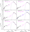 |
Fig. A.1. Observed SEDs obtained by combining Pan-STARRS, WIRCam, IRAC, SPIRE, SCUBA-2, and ALMA data (filled black circles) and best-fit templates (magenta curves) obtained with EAZY (Brammer et al. 2008) at the annotated photometric redshifts. The blue curve is the best-fit template at the spectroscopic redshift, available only for IDs 3 and 8. The green curve is the best-fit template to the Pan-STARRS-WIRCam-IRAC SED obtained using Hyper−z (Bolzonella et al. 2000) and the stellar population models of Bruzual & Charlot (2003). Single-temperature modified black-body models that fit the FIR-mm SED to within ±1σ are shown as solid purple curves, and dashed red or cyan curves for the warmer and cooler best fits. |
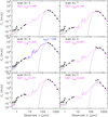 |
Fig. A.1. continued. |
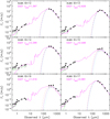 |
Fig. A.1. continued. |
All Tables
Deblended SCUBA-2 and Herschel-SPIRE flux densities for the individual ALMA-detected galaxies.
Pan-STARSS (Cols. 2–6), WIRCam (Cols. 7 and 8), and IRAC (Cols. 9 and 10) data.
All Figures
|
Fig. 1. Three-colour SPIRE image for G073.4−57.5 (reproduced from Planck Collaboration Int. XXVII 2015): blue, 250 μm; green, 350 μm; and red, 500 μm. The white contour shows the region encompassing 50% of the Planck flux density, while the yellow contours are the significance of the overdensity of red (350 μm) sources, plotted starting at 2σ with 1σ incremental steps. The rectangular area covering the ALMA pointings shown in Fig. 2 is highlighted in green. |
| In the text | |
|
Fig. 2. Central region (5.8′ × 4.6′) of G073.4−57.5 in a 3-colour image of Spitzer-IRAC 3.6 μm (red), combined CFHT-WIRCam/VLT-HAWKI K-band (green) and J-band (blue), with Herschel-SPIRE 250 μm contours in yellow (from 0.02 Jy beam−1 in 0.0125 Jy beam−1 steps) and ALMA galaxy positions shown with green circles of radius 3″ (enlarged by a factor of 12 from ALMA’s synthesised beam for clarity), labelled according to their source IDs given in Table 2. The ALMA areas that were used for the analysis (0.2 times the primary-beam peak response) are indicated with white circles (37″ diameter), labelled according to their field IDs given in Table 2. Four SCUBA-2 sources centred in the cyan circles (13″ diameter, matching the beam size) are labelled according to MacKenzie et al. (2017); the two SCUBA-2 sources labelled “4+/5+” are additionally selected as > 3σ peaks in the SCUBA-2 maps coincident with ALMA-detected sources. ALMA field 5 (with one detected source, see Fig. 3) is located above and to the right of the central region and is not shown in this image. |
| In the text | |
|
Fig. 3. Spitzer channel-2 postage stamps (30″ × 30″, with 2″ angular resolution) in grey scale (from 0.35 to 0.6 MJy sr−1) of the eight ALMA fields. White contours show the Herschel 250 μm surface brightness (from 0.01 Jy beam−1 in 0.005 Jy beam−1 or 1σ steps). Green contours represent the ALMA surface brightness (from 0.12 mJy beam−1 in 0.06 mJy beam−1 or 1σ steps). The detected ALMA galaxies are labelled with 1″ radius magenta circles, their photometric redshifts derived in Sect. 5 (or spectroscopic redshifts for ALMA IDs 3 and 8, Sect. 6) are given in white, and the ALMA fields are numbered in blue. |
| In the text | |
|
Fig. 4. Left: colour ([3.6] − [4.5]) versus magnitude ([4.5]) diagram for IRAC sources (red points) located within 1′ of SPIRE source 11, and for all the ALMA sources (blue stars); “[3.6]” means “channel 1” and “[4.5]” is “channel 2”. Numbers indicate the ALMA source IDs, as in Table 1. The black dashed line indicates a colour of −0.1 (red sources are defined to have colours above this value), the red line indicates the median colour of IRAC red sources within 1′ of SPIRE source 11 (0.14 mag), and the blue line indicates the median colour for the ALMA sources matched to IRAC red sources (0.27 mag). The dispersions around these median values are 0.15 and 0.13 mag, respectively (the latter is indicated by the blue region). The solid black line indicates the colour of a single stellar population formed at zf = 5, passively evolved to redshift z = 1.5 (from Bruzual & Charlot 2003), but extinction and possible metallicity effects have not been considered. Most ALMA sources lie on a sequence in this colour-magnitude plane, a characteristic feature of high-z structures (e.g. Muzzin et al. 2013; Rettura et al. 2014). We note that ALMA ID 14 is not plotted here, because it was not detected in the Spitzer-IRAC data. Right: normalised distribution of the colour of IRAC sources: the red line corresponds to sources within 1′ of SPIRE source 11; the blue line shows the ALMA sources; and the black dashed line shows the distribution of the colours of general sources in the COSMOS field for comparison. There is a significant excess of red galaxies around SPIRE source 11, in particular for the ALMA detections (further details in the text). |
| In the text | |
|
Fig. 5. Spitzer-IRAC versus CFHT WIRCam colour-colour diagram, with a track drawn from Bruzual & Charlot (2003) for a 1.4 Gyr simple stellar population, numbered by redshift. The horizontal and vertical dashed lines indicate the Papovich (2008) and Franx et al. (2003) criteria, respectively, representing colours of z ≃ 1.3 and z ≃ 2 galaxies (cf. the labels on the model curve). A redshift around z = 1.6–2.6 is indicated for the majority of the ALMA galaxies. Arrows represent 2σ limits for the sources not detected in any channel or band. |
| In the text | |
|
Fig. 6. Photometric redshift distribution of the maximum-likelihood solutions (filled red histogram) and combined probability density function (PDF, i.e. sum of the individual source likelihoods; solid blue curve) obtained with EAZY for all ALMA galaxies in the G073.4−57.5 field. Both the single photo-z distribution and the combined PDF of the ALMA sources show two clear redshift concentrations, one at z ≃ 1.5 and the other at z ≃ 2.4 (indicated by the vertical dashed lines). |
| In the text | |
|
Fig. 7. Stellar mass as a function of photometric redshift for the 18 ALMA galaxies. The green rectangles represent the expected values of the characteristic mass ℳ* and their uncertainties obtained by fitting the mass function of SFGs with a Schechter function in the redshift ranges 0.2–0.5, 0.5–0.8, 0.8–1.1, 1.1–1.5, 1.5–2.0, 2.0–2.5, 2.5–3.0, 3.0–3.5, and 3.5–4.0 (Davidzon et al. 2017). The source IDs are labelled next to the corresponding symbols. |
| In the text | |
|
Fig. 8. “Starburstiness”, which is the ratio of the star-formation rate to the SFR expected for a source on the MS (using the relation at the respective redshift), plotted against redshift. A factor of 3 around the MS is indicated by the grey region. Stars highlight galaxies assumed to be at z ≃ 1.54. |
| In the text | |
|
Fig. 9. Spectra of the two ALMA galaxies ID 3 (top and middle) and ID 8 (bottom), showing the serendipitous line detections, consistent with a CO(5–4) transition at z = 1.54. The blue Gaussian profiles show the best fits to each individual line. The red Gaussian profiles for ID 3 show the best combined fit to the CO(5–4) line in the ALMA spectrum (top) and the CO(2–1) line in the IRAM/EMIR spectrum (middle). The offset between the fitted line centres seen in the EMIR data is small, 66 km s−1, and could be due to the low S/N, the edge of the ALMA spectral window, or a physical difference between the transitions. Representative error bars per bin are shown for every third bin. We note that we have applied the standard flagging of edge channels in the ALMA spectral window for ID 3, which otherwise could introduce systematic uncertainties. |
| In the text | |
|
Fig. 10. Images for ID 3 (on the left) and ID 8 (on the right) of the integrated line emission in Jy km s−1 beam−1 (where the continuum has been subtracted). In both cases line and continuum emission (i.e. the black contours from 3σ = 0.18 mJy in 3σ steps) coincide. The middle panel shows (for the stronger line of ID 3 only) the first-moment image in km s−1, along with continuum contours for reference. The FWHM of the synthesised beam (0.56″ × 0.44″) is shown with red ellipses and a 5 kpc bar is shown in black for reference. |
| In the text | |
|
Fig. 11. SFE (≡ |
| In the text | |
|
Fig. 12. SFE normalised to the expected SFE assuming the relation valid for MS galaxies from Eq. (5) as a function of offset from the MS (starburstiness) for ALMA IDs 3 and 8 (filled stars), and for sources from the literature with 1 < z < 3 (filled squares: cluster galaxies, filled triangles: proto-cluster galaxies). The horizontal and vertical solid lines represent, respectively, SFEs and starburstiness values of MS galaxies, and the grey region indicates SFRs consistent with the MS within a factor of 3. |
| In the text | |
|
Fig. 13. Molecular gas mass, derived from the CO luminosity (in red if αCO = 0.8, and in blue if αCO = 4.0–4.36), as a function of LIR for ALMA IDs 3 and 8 (filled stars) and galaxies in clusters (filled squares) or in proto-clusters (filled triangles). Gas masses refer to ISM masses derived from the mm continuum for all ALMA sources (green open stars with annotated IDs). The solid and dashed lines represent the expected relations for MS and SB galaxies, respectively, as derived from Eqs. (5) and (6), and assuming αCO = 4.36 (for MS galaxies) or 0.8 (for SB galaxies, SFR > 3 × SFRMS for our sample) (Sargent et al. 2014). The grey areas represent 1σ uncertainties in the theoretical parameters of the relations. |
| In the text | |
|
Fig. 14. Gas fraction fgas = Mgas/(Mgas + ℳ) as a function of ℳ. The symbols are defined as in Fig. 13. The solid and dashed curves represent the expected relations for MS and SB galaxies, respectively, at z = 1.5 (cyan) and at z = 2.5 (orange). |
| In the text | |
|
Fig. 15. Normalised molecular gas mass fraction μmol ≡ Mgas/ℳ as a function of the normalised SFR. The symbols are defined as in Fig. 13. The black solid curve and grey area represent the values predicted by the 2-SFM framework described in Sargent et al. (2014). Sources with ℳ > 1011 M⊙ are shown with magenta large squares. The grey area shows the expected 1σ scatter around the average molecular gas mass fraction. |
| In the text | |
|
Fig. A.1. Observed SEDs obtained by combining Pan-STARRS, WIRCam, IRAC, SPIRE, SCUBA-2, and ALMA data (filled black circles) and best-fit templates (magenta curves) obtained with EAZY (Brammer et al. 2008) at the annotated photometric redshifts. The blue curve is the best-fit template at the spectroscopic redshift, available only for IDs 3 and 8. The green curve is the best-fit template to the Pan-STARRS-WIRCam-IRAC SED obtained using Hyper−z (Bolzonella et al. 2000) and the stellar population models of Bruzual & Charlot (2003). Single-temperature modified black-body models that fit the FIR-mm SED to within ±1σ are shown as solid purple curves, and dashed red or cyan curves for the warmer and cooler best fits. |
| In the text | |
|
Fig. A.1. continued. |
| In the text | |
|
Fig. A.1. continued. |
| In the text | |
Current usage metrics show cumulative count of Article Views (full-text article views including HTML views, PDF and ePub downloads, according to the available data) and Abstracts Views on Vision4Press platform.
Data correspond to usage on the plateform after 2015. The current usage metrics is available 48-96 hours after online publication and is updated daily on week days.
Initial download of the metrics may take a while.