| Issue |
A&A
Volume 620, December 2018
The XXL Survey: second series
|
|
|---|---|---|
| Article Number | A5 | |
| Number of page(s) | 28 | |
| Section | Cosmology (including clusters of galaxies) | |
| DOI | https://doi.org/10.1051/0004-6361/201731606 | |
| Published online | 20 November 2018 | |
The XXL Survey
XX. The 365 cluster catalogue★,★★
1
Aix Marseille Univ., CNRS, CNES, LAM,
Marseille,
France
e-mail: This email address is being protected from spambots. You need JavaScript enabled to view it.
2
INAF – Osservatorio astronomico di Padova,
Vicolo Osservatorio 5,
35122
Padova,
Italy
3
Laboratoire AIM, CEA/DSM/IRFU/SAp, CEA Saclay,
91191
Gif-sur-Yvette,
France
4
Argelander Institut für Astronomie, Universität Bonn,
Auf dem Hügel 71,
53121
Bonn,
Germany
5
European Southern Observatory,
Alonso de Cordova 3107, Vitacura,
19001
Casilla,
Santiago 19,
Chile
6
Departamento de Astronomía, DCNE-CGT, Universidad de Guanajuato; Callejón de Jalisco,
s/n, Col. Valenciana,
36240
Guanajuato,
Gto.,
Mexico
7
School of Physics, HH Wills Physics Laboratory,
Tyndall Avenue,
Bristol
BS8 1TL,
UK
8
INAF – IASF Milano,
via Bassini 15,
20133
Milano,
Italy
9
Department of Astronomy, University of Geneva,
Ch. d’Écogia 16,
1290
Versoix,
Switzerland
10
Aristotle University of Thessaloniki, Physics Department,
Thessaloniki
54124,
Greece
11
Australian Astronomical Observatory,
PO Box 915,
North Ryde
1670,
Australia
12
Laboratoire Lagrange, UMR 7293, Université de Nice Sophia Antipolis, CNRS, Observatoire de la Côte d’Azur,
06304
Nice,
France
13
Department of Physics, University of Oxford,
Oxford
OX1 3PU,
UK
14
Merton College,
Oxford
OX1 4JD,
UK
15
School of Physics and Astronomy, University of Nottingham,
University Park,
Nottingham
NG7 2RD,
UK
16
Astrophysics and Space Research Group, School of Physics and Astronomy, Univ. of Birmingham,
Birmingham
B15 2TT,
UK
17
Macquarie University,
NSW
2109,
Australia
18
ICRAR,
1 Turner Avenue,
Technology Park, Bentley,
Western Australia
6102,
Australia
19
University of St Andrews,
College Gate, St Andrews,
KY16 9AJ
Fife,
UK
20
Astrophysics Research Institute, Liverpool John Moores Univ., IC2, Liverpool Science Park,
146 Brownlow Hill,
Liverpool
L3 5RF,
UK
21
Monash University,
Victoria
3800,
Australia
22
Hamburger Sternwarte, Universität Hamburg,
Gojenbergsweg 112,
21029
Hamburg,
Germany
23
Max-Planck-Institut für Kernphysik,
PO Box 103980,
69029
Heidelberg,
Germany
24
Max-Planck-Institut für Kernphysik,
Saupfercheckweg 1,
69117
Heidelberg,
Germany
25
Department of Astronomy, University of Michigan,
Ann Arbor,
MI
48109,
USA
26
Department of Physics, University of Michigan,
Ann Arbor,
MI
48109,
USA
27
INAF, Osservatorio Astronomico di Bologna,
via Pietro Gobetti 93/3,
40129
Bologna,
Italy
28
Chalmers University of Technology, Department of Space, Environment, and Earth, Onsala Space Observatory,
439 92
Onsala,
Sweden
29
INAF – Osservatorio Astronomico di Brera,
Via Brera 28, 20122 Milano, via E. Bianchi 46,
20121
Merate,
Italy
30
Department of Physics and Astronomy, University of Victoria,
3800 Finnerty Road,
Victoria,
BC
V8P 1A1,
Canada
31
Department of Physics and Astronomy, University of Padova,
Vicolo Osservatorio 3,
35122
Padova,
Italy
32
European Space Astronomy Centre (ESA/ESAC), Operations Department,
Villanueva de la Canãda,
Madrid,
Spain
33
Univ. degli studi di Milano,
via G. Celoria 16,
20133
Milano,
Italy
34
Dipartimento di Fisica e Astronomia (DIFA), Università di Bologna,
viale Berti Pichat 6/2,
40127
Bologna,
Italy
35
INFN, Sezione di Bologna,
viale Berti Pichat 6/2,
40127
Bologna,
Italy
36
National Centre for Nuclear Research,
ul. Hoza 69,
00-681
Warszawa,
Poland
37
IRAP Université de Toulouse, CNRS, UPS,
Toulouse,
France
38
Astronomical Observatory of the Jagiellonian University,
Orla 171,
30-001
Cracow,
Poland
39
INAF – IASF Bologna,
via Gobetti 101,
40129
Bologna,
Italy
40
Aix-Marseille Université – Pharo,
58 bd Charles Livon Jardin du Pharo,
13007
Marseille,
France
41
Department of Astronomy and Space Sciences, Faculty of Science, Istanbul University,
34119
Istanbul,
Turkey
42
INFN, Sezione di Bologna,
viale Berti Pichat 6/2,
40127
Bologna,
Italy
43
Center for Astrophysics and Space Astronomy, Department of Astrophysical and Planetary Science, University of Colorado,
Boulder,
CO
80309,
USA
44
NASA Ames Research Center,
Moffett Field,
CA
94035,
USA
45
National Observatory of Athens,
Lofos Nymfon,
11851
Athens,
Greece
46
Centre for Extragalactic Astronomy, Department of Physics, Durham University,
South Road,
Durham
DH1 3LE,
UK
Received:
20
July
2017
Accepted:
27
November
2017
Abstract
Context. In the currently debated context of using clusters of galaxies as cosmological probes, the need for well-defined cluster samples is critical.
Aims. The XXL Survey has been specifically designed to provide a well characterised sample of some 500 X-ray detected clusters suitable for cosmological studies. The main goal of present article is to make public and describe the properties of the cluster catalogue in its present state, as well as of associated catalogues of more specific objects such as super-clusters and fossil groups.
Methods. Following from the publication of the hundred brightest XXL clusters, we now release a sample containing 365 clusters in total, down to a flux of a few 10−15 erg s−1 cm−2 in the [0.5–2] keV band and in a 1′ aperture. This release contains the complete subset of clusters for which the selection function is well determined plus all X-ray clusters which are, to date, spectroscopically confirmed. In this paper, we give the details of the follow-up observations and explain the procedure adopted to validate the cluster spectroscopic redshifts. Considering the whole XXL cluster sample, we have provided two types of selection, both complete in a particular sense: one based on flux-morphology criteria, and an alternative based on the [0.5–2] keV flux within 1 arcmin of the cluster centre. We have also provided X-ray temperature measurements for 80% of the clusters having a flux larger than 9 × 10⁻¹⁵ erg s−1 cm−2.
Results. Our cluster sample extends from z ~ 0 to z ~ 1.2, with one cluster at z ~ 2. Clusters were identified through a mean number of six spectroscopically confirmed cluster members. The largest number of confirmed spectroscopic members in a cluster is 41. Our updated luminosity function and luminosity–temperature relation are compatible with our previous determinations based on the 100 brightest clusters, but show smaller uncertainties. We also present an enlarged list of super-clusters and a sample of 18 possible fossil groups.
Conclusions. This intermediate publication is the last before the final release of the complete XXL cluster catalogue when the ongoing C2 cluster spectroscopic follow-up is complete. It provides a unique inventory of medium-mass clusters over a 50 deg2 area out to z ~ 1.
Key words: galaxies: clusters: general / large-scale structure of Universe / galaxies: groups: general / galaxies: clusters: intracluster medium
Based on observations obtained with XMM-Newton, an ESA science mission with instruments and contributions directly funded by ESA Member States and NASA. Based on observations made with ESO Telescopes at the La Silla and Paranal Observatories under programmes ID 191.A-0268 and 60.A-9302. Based on observations obtained with MegaPrime/MegaCam, a joint project of CFHT and CEA/IRFU, at the Canada-France-Hawaii Telescope (CFHT) which is operated by the National Research Council (NRC) of Canada, the Institut National des Sciences de l’Univers of the Centre National de la Recherche Scientifique (CNRS) of France, and the University of Hawaii. Based on observations collected at the German-Spanish Astronomical Centre, Calar Alto, jointly operated by the Max-Planck-Institut für Astronomie Heidelberg and the Instituto de Astrofísica de Andalucía (CSIC). This work is based in part on data products produced at Terapix available at the Canadian Astronomy Data Centre as part of the Canada-France-Hawaii Telescope Legacy Survey, a collaborative project of NRC and CNRS. This research has made use of the VizieR catalogue access tool, CDS, Strasbourg, France. This research has also made use of the NASA/IPAC Extragalactic Database (NED) which is operated by the Jet Propulsion Laboratory, California Institute of Technology, under contract with the National Aeronautics and Space Administration.
Full Table 5 is only available at the CDS via anonymous ftp to cdsarc.u-strasbg.fr (130.79.128.5) or via http://cdsarc.u-strasbg.fr/viz-bin/qcat?J/A+A/620/A5
© ESO 2018
1 Introduction
Most galaxycluster-related cosmological probes rely on cluster number counts and large-scale structure information. X-ray surveys have had a key role in this framework since the historical Einstein observatory Medium Sensitivity Survey (Gioia et al. 1990). Many other surveys were conducted with the ROSAT observatory, and more recently, XMM-Newton and Chandra produced surveys such as the XMM-LSS, XMM-COSMOS, XMM-CDFS and Chandra-Ultra-Deep surveys (Pierre et al. 2004; Hasinger et al. 2007; Comastri et al. 2011; Ranalli et al. 2013). Following this path, it is now clear that cluster cosmological studies can only be rigorously performed by simultaneously fitting a cosmological model, the cluster selection function and the physical modelling of the cluster evolutionary properties in whichever band the cluster selection has been performed (e.g. Allen et al. 2011). X-ray cluster cosmology is especially well suited to such an approach, because the properties of the X-ray emitting intra-cluster medium can be ab-initio predicted with good accuracy, either using an analytical model or by means of hydrodynamical simulations.
The XMM-XXL project (XXL hereafter) covers two areas of 25 deg2 each with XMM-Newton observations to a sensitivity of ~ 5 × 10⁻¹⁵ erg s−1 cm−2 (for point sources); the two areas are centred at: XXL-N (02h 23′ −04°30′) and XXL-S (23h 30′ −55°00′). In a first step, XXL aims at in-depth cluster evolutionary studies over the 0 < z < 1 range by combining an extensive data set over the entire electromagnetic spectrum. In a second and ultimate step we aim at a standalone cosmological analysis (Pierre et al. 2016, hereafter XXL Paper I) and the X-ray cluster catalogue constitutes the core of the wholeproject: its construction along with the determination of the cluster multiwavelength parameters follows an iterative process demanding special care. In this process, the spectroscopic confirmation of the X-ray cluster candidates has occupied a central place in the project over the last 5 yr. In a first publication (Pacaud et al. 2016, hereafter XXL Paper II) we presented the hundred brightest galaxy clusters (XXL-100-GC) along with a set of preliminary scientific analyses, including the X-ray luminosity function, spatial correlation studies and a cosmological interpretation of the number counts. The present, and second, release is the last before the publication of the complete cluster catalogue. This will occur when the ongoing C2 cluster spectroscopic follow-up is completed. The main goal of present article is to make public and describe the properties of the second release, as well as of associated catalogues of more specific objects such as super-clusters and fossil groups. The present sample contains the complete subset of clusters for which the selection function is well determined (namely, the C1 selection) plus all X-ray clusters which are, to date, spectroscopically confirmed. The C1 and C2 classes are defined as in XXL Paper II and will be described below. Altogether, this amounts to 365 clusters and is referred to as the XXL-365-GC sample (cf. Table 1). Along with the cluster list itself, we provide an update of the X-ray cluster properties and of their spatial distribution as presented in the 2016 XXL-100-GC publications. The cluster parameters derived in the present publication supersede the XXL-100-GC ones, even thought the consistency (see below) is very good.
In the next section, we describe the construction of the current sample. Section 3 gives a detailed account of the spectroscopic validation procedure. We present the cluster catalogue in Sect. 4. Section 5 provides updated determinations of the X-ray cluster luminosity function and of the luminosity–temperature relation. The results of spatial analyses performed on the cluster catalogue (search for super-clusters and fossil groups) are presented in Sect. 6. Notes on the newly detected structures and recent redshift measurements are gathered in Appendices. Throughout the paper, for consistency with the first series of XXL papers, we adopt the WMAP9 cosmology (Hinshaw et al. 2013, with Ωm = 0.28, ΩΛ = 0.72, and H0 = 70 km s−1 Mpc−1), except if explicitly stated. From the semantic point of view, we also mention that the structures called clusters in the present paper are not very massive structures, but are intermediate-mass concentrations in the mass range between groups of galaxies and very massive clusters of galaxies.
Statistics of the XXL-365-GC, XXL-C1-GC, and XXL-100-GC samples.
2 Selection of the X-ray cluster sample
The X-ray pipeline and the cluster selection procedure along with the XXL selection function are extensively described in XXL Paper II. We recall here the main steps.
Our detection algorithm (the same version of Xamin used in XXL Paper II, cf. also Faccioli et al. 2018, hereafter XXL Paper XXIV) enables the creation of an uncontaminated (C1) cluster sample by selecting all detected sources in the 2D [EXT; EXT_STAT] output parameter space. The EXT parameter is a measure of the cluster apparent size and the EXT_STAT parameter quantifies the likelihood ofa source of being extended. The EXT_STAT likelihood parameter is a function of cluster size, shape and flux. This parameter depends on the local XMM-Newton sensitivity.
Simulations enable the definition of limits for EXT and EXT_STAT above which contamination from point sources is negligible, providing the C1 sample. Relaxing slightly these limits, we define a second, deeper, sample (C2) to allow for 50% contamination by misclassified point sources; these can easily be cleaned up a posteriori using optical versus X-ray comparisons. Initially, the total number of such C2 cluster candidates was 195 and more than 60% are already spectroscopically confirmed (see below). We defined a third class, C3, corresponding to (optical) clusters associated with some X-ray emission, too weak to be characterised; the selection function of the C3 sample is therefore undefined. Initially, most of the C3 objects were not detected in the X-ray waveband and are located within the XMM-LSS subregion. We refer the reader to Pierre et al. (2004) for a more detailed description of these classes.
With the present paper, we publish all C1 clusters (XXL-C1-GC hereafter, cf. Table 1) supplemented by the C2 and C3 clusters which are spectroscopically confirmed. C3 clusters were not specifically targeted, but were sometimes confirmed as by-products of existing galaxy spectroscopic surveys. Table 2 gives statistics of the XXL-365-GC sample in terms of C1, C2, and C3 clusters. This amounts to 207 C1 (among them, 183 spectroscopically confirmed to date, 4 with some spectroscopy but needing more data, 13 with a photometric redshift, and 7 without redshift estimation), 119 C2 and 39 C3. The C1 selection provides a complete sample in the two-parameter space outlined above. In order to allow straightforward comparisons with different X-ray processing methods, we give, for information only, the approximate completeness flux limit of the XXL-365-GC sample computed from simulated detections. We performed the measurements within a radius of 1 arcmin around the cluster centre (defined from the X-ray data). We assume, as in XXL Paper II, that the XMM-Newton count-rates are computed in the [0.5–2] keV band and converted into fluxes assuming an Energy Conversion Factor (ECF) of 9.04 × 10⁻¹³ erg s−1 cm−2/(cts/s). The completeness flux limit (the 100% completeness flux limit averaged across the entire survey area) is then ~1.3 × 10⁻¹⁴ erg s−1 cm−2. We emphasise that since a flux of 10−14 corresponds to ~100 photons on-axis for 10 ks exposures (MOS1 + MOS2 + PN), uncertainties are large, which may affect the cluster ranking as a function of the flux by 10% or more.
Statistics of the XXL-365-GC sample in terms of C1, C2, and C3 clusters.
3 Spectroscopic redshifts
3.1 Collecting the spectroscopic information
The spectroscopic surveys conducted on the XXL fields are listed in XXL Paper I (Table 3). We provide below a short description of this rather heterogeneous data set. In order to perform the spectroscopic validation and further dynamical studies of the XXL clusters, all available spectroscopic information on galaxies located in the XXL fields has been stored in the CEntre de donnéeS Astrophysiques de Marseille1. Their astrometry was matched with the CFHTLS T0007 catalogue2 for XXL-N and with the BCS catalogue (Desai et al. 2012) for XXL-S. The public and private surveys stored in CESAM and relevant to XXL are described in the following. All in all, the total number of redshifts present in the CESAM database are ~145 000 and ~8500 for the XXL-N and XXL-S fields respectively (as of December 2016, including multiple measurements).
Details of the three ESO PI runs.
3.1.1 XXL extended sources spectroscopic follow-up campaigns
We conducted our own spectroscopic follow-up to complement the already available public spectroscopic data sets. C1 clusters were the primary targets, but we also targeted C2 clusters when possible. The targets were chosen in order to favour the cluster confirmation by galaxies within the X-ray contours. We note that the X-ray contours are created from a wavelet filtered photon image. The contours are run in each frame for the range between 0.1 cts/px corresponding to the typical background level for exposition time of 10 ks (~10−5 cts/s/px) and a maximal value in the frame spaced by 15 logarithmic levels.
- (a)
We made extensive use of the ESO optical facilities (NTT/EFOSC2 and VLT/FORS2). We were granted three PI allocations, including a Large Programme (191-0268) and a pilot programme (089.A-0666). We give the details of these new PI ESO programmes in Table 3.
FORS2 and EFOSC2 galaxy targets were first choosen according to their strategical place inside the clusters, taking into account the already known redshifts from other surveys, and their location regarding the X-ray contours. Then, we put as many slits as possible on other objects. We measured the spectroscopic redshifts by means of the EZ code (Garilli et al. 2008) that was already used for the VIPERS survey (Guzzo et al. 2014; Scodeggio et al. 2017). We adopted the same approach: the only operation that required human intervention is the verification and validation of the EZ measured redshift. Each spectrum is independently measured by two team members. At the end of the process, discrepant redshifts are discussed and homogenised. The quality of the redshift measurements is defined as in the VVDS and VIPERS surveys:
Flag 0: no reliable spectroscopic redshift measurement;
Flag 1: tentative redshift measurement with a ~50% chance that the redshift is wrong. These redshifts are not used;
Flag 2: confidence estimated to be >95%;
Flag 3 and 4: highly secure redshift. The confidence is estimated to be higher than 99%;
Flag 9: redshift based on a single clear feature, given the absence of other features. These redshifts are generally reliable.
- (b)
We also made use of the AAOmega instrument on the AAT. A first observing campaign was published in Lidman et al. (2016, hereafter XXL Paper XIV), while supplementary observations done in 2016 will be included in Chiappetti et al. (2018, hereafter XXL Paper XXVII). For the first run, cluster galaxies were the prime targets and we used Runz (Hinton et al. 2016) to measure redshifts. X-ray AGN in the XXL-S field were the prime targets for the second run and only spare fibres were put on cluster galaxies. We used Marz (Hinton et al. 2016) to measure redshifts. For each spectrum, we assign a quality flag that varies from 1 to 6. The flags are identical to those used in the OzDES redshift survey (Yuan et al. 2015). We used AAT quality flags 3 or 4 which are equivalent to the ESO flags 2, 3, or 4.
- (c)
We also obtained Magellan spectroscopy at Las Campanas observatory from an associated survey (A. Kremin, priv. comm.). We only used the 262 most reliable redshifts.
- (d)
We collected redshifts at the William Herschel Telescope (WHT hereafter, cf. Koulouridis et al. 2016, hereafter XXL Paper XII). Redshifts were measured and quality flags were assigned in the same way as for the ESO data.
3.1.2 Redshifts from the XMM-LSS survey
We included all redshifts obtained for the XMM-LSS pilot survey (11 deg2 precursor and subarea of XXL-N, Pierre et al. 2004). The sample is described in Adami et al. (2011).
3.1.3 Literature data
The XXL-N area was defined to overlap with the VIPERS survey (VIMOS Public Extragalactic Redshift survey: Guzzo et al. 2014; Scodeggio et al. 2017) and to encompass the VVDS survey (Le Fèvre et al. 2013). We therefore included the redshifts from these VIMOS-based redshift surveys. The redshifts are measured in our own ESO spectroscopic follow-up exactly in the same way as VIPERS and VVDS did, with the same quality flags. We also note that all redshifts from VIPERS, covering the redshift range 0.4 ≤ z ≤ 1.2, were made available for this analysis prior to the recent public release (Scodeggio et al. 2017).
GAMA, 2dF, 6dF, SDSS: These four catalogues were ingested and used without remeasuring the redshift of the galaxies. They provide robust spectroscopic quality flags. We considered as reliable the GAMA, 2dF, and 6dF redshifts with quality flags 3 and 4 (e.g. Liske et al. 2015 and Baldry et al. 2014 for GAMA, and Folkes et al. 1999 for 2dF), equivalent to the ESO flags 2, 3 or 4. SDSS spectra with “zWarning” between 0 and 16 were also used. We note that the GAMA spectroscopy inside the XXL area is issued from the GAMA G02 field where fibres were also intentionally put on preliminary proposed XXL galaxy targets. G02 will be public within the GAMA DR3 data release (Baldry et al., in prep.).
In addition, we considered other smaller public redshift catalogues: Akiyama et al. (2015) from Subaru, Simpson et al. (2006, 2012), Stalin et al. (2010), SNLS survey (e.g. Balland et al. 2009). We remeasured and checked the redshift values for these surveys, when spectra were available, using the methods developed for our own spectroscopic follow-up. We finally collected and assumed as correct all other redshifts on the XXL areas, currently available in the NED database.
3.2 Redshift reliability and precision
Our spectroscopic redshift catalogues come from various telescopes, with different instruments, different setups and were obtained under different observing conditions. We thus needed to evaluate on an objective basis the overall reliability of the data set. Although we tried to limit multiple observations, we ended up with a non-negligible number of galaxies present in different surveys. We used these redundant measurements to evaluate the statistical reliability of our redshifts. The simplest approach consists in plotting the redshift difference versus redshift (cf. Fig. 1) for the ~12 000 objects measured twice in the whole spectroscopic sample. Out of these, 15% had a spectroscopic quality flag of 4, 61% a quality flag of 3, 24% a quality flag of 2, and <1% a quality flag of 9. We only consider flags >2 in the following.
- (a)
To estimate the fraction of incompatible redshifts, we selected in Fig. 1 all double measurements differing by more than ±3 × 600 km s−1 (600 km s−1 is a typical value based on the VVDS and VIPERS surveys: cf. Le Fèvre et al. 2013 and representing a good compromise between the spectrographs resolution and the possible real difference between redshifts, at the 3-σ level). This points to strongly discrepant redshifts for 5% of the sample. A comparable percentage is expected in Guzzo et al. (2014) for the VIPERS survey. We therefore conclude that our sample is similar to the VIPERS survey in terms of incompatible redshifts (cf. Scodeggio et al. 2017).
- (b)
For measurements within ±3 × 600 km s−1, the statistical 1-σ redshift scatter is ~0.00049 × (1 + z). This represents almost 150 km s−1. We note that Fig. 1 may give the feeling that the dispersion is much larger at low redshifts. However, this is mainly due to the fact that many objects are concentrated along the zero difference level. The statistical 1-σ uncertainty is for example ~0.00049 at z ≤ 1 and ~0.00057 at z ≤ 0.5.
- (c)
The previous estimates pertain to the full galaxy sample. We also performed a similar analysis on the cluster galaxies alone. These galaxies have different types and luminosities and are therefore potentially subject to different selections. To select these galaxies, we limited the sample to galaxies within one Virial radius and with a velocity within ± 3 × σv,200, the equivalent galaxy velocity dispersion inferred from scaling laws within the Virial radius, from the cluster centre. We could have tried to use instead the galaxy velocity dispersion computed with galaxy redshifts, but our sampling is too sparse to have precise estimations. This will be treated in a future paper. Virial radius and σv,200 were estimated from X-ray data given in Table F.1 and described in the following. Applying the same method as with the complete sample, we find an incompatible redshift percentage of ~4% (cf. Fig. 2), even better than for the total sample. The 1-σ redshift scatter is ~0.00041 × (1 + z), or 120 km s−1 in termsof radial velocity uncertainty, also similar to the estimate for the total sample. Finally, we do not see any significant variation of the 1-σ uncertainty between redshifts 0 and 0.9.
The last issue is to estimate the relative weight of the various telescopes in the cluster redshift compilation. Considering the sample of cluster galaxies only, we find that ~45% are coming from ESO (VIMOS and FORS2 instruments), ~45% from AAT (AAOmega instrument), and ~7% from SDSS. The remaining ~3% have variousorigins (Subaru, WHT, LasCampanas, etc.).
As a remark, for a given object with multiple redshift measurements, we used the measurement coming from the highest quality spectrum. We did not notice systematic redshift differences in the considered surveys.
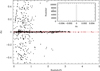 |
Fig. 1 Redshift difference versus redshift for the ~12 000 objects measured twice within the spectroscopic survey. The two red dotted lines represent the ±3 × 600 km s−1 level (cf. Sect. 3.2). We also give the histogram of the redshift difference within the [− 0.005, 0.005] interval. |
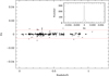 |
Fig. 2 Redshift difference versus redshift for the galaxies (at < ± 3 × σv,200 from the cluster mean redshift and within one Virial radius) measured two times within the spectroscopic survey. The two red dotted lines represent the ±3 × 600 km s−1 level. We also give the histogram of the redshift difference within the [− 0.005, 0.005] interval. |
3.3 Cluster spectroscopic confirmation
Starting from the list of extended X-ray sources (C1 or C2), the cluster spectroscopic confirmation is an iterative process.
- (1)
We first collected all available spectroscopic redshifts along a given line of sight towards a cluster candidate. We selected the spectroscopic redshifts within the X-ray contours and searched for gaps larger than 900 km s−1 in the resulting redshift histogram. This is intended to separate different concentrations in the redshift space. We searched for concentrations of three or more redshifts between two gaps and preliminarily assigned the largest concentration to the extended source in question. This allows us to estimate the angular distance of the source in question.
- (2)
We then repeated the process, this time within a 500 kpc radius. This has sometimes led us to consider larger regions than the ones defined by the X-ray contours. We checked whether the inferred redshift was compatible with the previous one. If yes, we considered the cluster to be confirmed at the considered redshift. If not, we restarted the full process with another redshift concentration. In practice, this process was convergent at the first pass for the large majority of the cases.
We kept open the possibility of manually assigning a redshift to a cluster when the two previous criteria did not agree (cf. below the peculiar case of XLSSC 035). This mainly occurred when dealing with projection effects alongthe line of sight (cf. the eight cases in Appendix B). Some of the lines of sight were however poorly sampled, with typically fewer than three redshifts. In this case, we attempted to confirm the cluster nature of the X-ray source by identifying the cluster dominant galaxy (BCG hereafter) in the i′ band and close to the X-ray centroid. If the choice of such a galaxy was obvious and this galaxy had a spectroscopic redshift, we confirmed the cluster as well. This was the case for 30 clusters (with only the BCG), and for another 50 clusters (with the BCG plus another concordant galaxy).
The C3 clusters – X-ray sources too faint to be characterised as C1 or C2 – that we present in this paper are only those resulting from the spectroscopic follow-up of X-ray sources in the XMM-LSS pilot survey. We did not perform any systematic cluster search or follow-up for the full list of X-ray sources.
In Fig. 3, we give the contribution of the major spectroscopic surveys used in the present paper. This is showed both in terms of the number of clusters with a given number of galaxy redshifts coming from a given spectroscopic survey, and in terms of number of galaxy redshifts coming from a given survey for a given redshift bin. This for example shows that the XXL ESO and XMM-LSS PI allocations were efficient to confirm clusters in the z ~ [0.2–1] range while other major surveys were more specialised in terms of redshift coverage: VIPERS at z ≥ 0.45, and AAT PI and GAMA at z ≤ 0.7 and z ≤ 0.4 respectively. In terms of cluster spectroscopic sampling, XXL ESO PI allocations enabled us to measure the largest number of galaxy redshifts per cluster (~5); other surveys yielded various samplings. The largest samplings are achieved by the XMM-LSS spectroscopic survey (most of the time for well identified peculiar or distant clusters) and by the GAMA spectroscopic survey for nearby clusters.
Major surveys such as VIPERS or GAMA have science objectives related to field studies, and are therefore under-represented in Fig. 3 because only a small fraction of these redshifts falls within a given cluster. We therefore give in Table 4the mean numbers of redshifts per line of sight (over the full redshift range of the XXL Survey, and within angular radii corresponding to 500 kpc at the redshifts of the clusters). This allows us to appreciate the respective contribution of these surveys to the characterisation of both clusters and projection effects. In such a table, intensive field surveys as VIPERS or GAMA show their great importance.
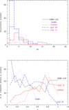 |
Fig. 3 Upper panel: y-axis, number of confirmed clusters; x-axis, number of galaxy redshifts sampling the confirmed clusters. Different colours and line styles are from different spectroscopic surveys. Bottom panel: percentage of galaxy redshifts inside the confirmed clusters coming from a given survey and for a given redshift bin. Because of multiple galaxy spectroscopic measurements, the sum of the percentages for a given redshift bin is larger than 100%. |
4 The cluster catalogue
In this section, we first provide a global description of the sample. We then present the direct (spectral) measurements we made of luminosity, temperature, gas mass, and flux. These measurements are obviously more robust than using scaling relations, but they require higher quality data and therefore cannot be computed for the whole sample of clusters. Scaling relations were therefore used in order to complete the sample for some of the following studies.
4.1 Sample description
The C1 + C2 clusters are listed in Table 5 which is sorted according to increasing RA and only the first twenty entries are displayed. Blank places in the table are undetermined values. We note that the XLSSC 634 cluster was confirmed by Ruel et al. (2014) with Gemini/GMOS data. The spectroscopically confirmed C3 objects are listed in Table G.1. Both tables are also available in the XXL Master Catalogue browser3 and Table 5 is available at the CDS. For each source, we provide (when available):
-
the XLSSC identifier (between 1 and 499, or 500 and 999 for XXL-N or XXL-S respectively;
-
RA and Dec;
-
the redshift and the number of galaxies used for the redshift determination;
-
basic X-ray and X-ray related quantities for the clusters of the present release (X-ray fluxes, Mgas,500 kpc, r500,MT, T300 kpc, and
 ). We note that we give in the present paper the value of Mgas,500 kpc, contraryto what was given in XXL Paper XIII;
 -
a flag indicating whether there is a note on the cluster in Appendix G, whether the cluster was already published in XXL Paper II or in former XMM-LSS releases, and whether the cluster is a member of the flux limited sample.
4.2 X-ray direct measurements
4.2.1 Luminosity and temperature
Full details of the analysis of the cluster X-ray properties will be found (Giles et al., in prep.), and we outline the main steps of the spectral analysis here. First, we only used the single best pointings for spectral analyses when sources fell on multiple pointings. As a conservative approach, the extent of the cluster emission was defined as the radius beyond which no significant cluster emission is detected using a threshold of 0.5σ above the background level. Due to the low number of counts and low signal-to-noise ratio (S/N) of many of the clusters below the XXL-100-GC threshold, we performed a detailed modelling of the background, instead of a simple background subtraction. We followed the method outlined in Eckert et al. (2011), who performed this detailed modelling to study a source whose emission barely exceeded the background. We modelled the non X-ray background (NXB) using closed filter observations, following a phenomenological model. For observations contaminated by soft protons (where the count rate ratio between the in-FOV, beyond 10 arcmin, and out-of-FOV regions of the detector was >1.15), we included an additional broken power-law component, with the slopes fixed at 0.4 and 0.8 below and above 5 keV respectively. The sky background was modelled using data extracted from an offset region (outside the cluster emission determined above), using a three-component model as detailed in Eckert et al. (2011). Within the XSPEC environment, cluster source spectra were extracted for each of the XMM-Newton cameras and fits were performed in the [0.4–11.0] keV band with an absorbed APEC (Astrophysical Plasma Emission Code, Smith et al. 2001) model (v2.0.2), with a fixed metal abundance of Z = 0.3 Z⊙.
We denote the luminosity within r500,MT4 as  , within the [0.5–2.0] keV band (cluster rest frame). Luminosities quoted within r500,MT are extrapolated from 300 kpc (see below) out to r500,MT by integrating under a β-profile assuming a core radius rc = 0.15r500,MT and an external slope β = 0.667 (cf. XXL Paper II). Values for cluster r500,MT are calculated using the mass–temperature relation of Lieu et al. (2016, hereafter XXL Paper IV).
Given that we are dealing with much fainter sources than in XXL Paper II, it was not possible to measure X-ray temperatures for all clusters. In particular, several C1 clusters were located in pointings affected by flaring, had very low counts, were contaminated by point sources, or were at very low redshift so with a bad spatial coverage.
4.2.2 Gas mass
We analytically computed gas masses for clusters with redshifts following closely the method outlined in Eckert et al. (2014, hereafter XXL Paper XIII). Here we briefly recall the various steps of the analysis. First, we extract surface-brightness profiles in the [0.5–2] keV band starting from the X-ray peak using the PROFFIT package (Desai et al. 2012). We compute the surface-brightness profiles from mosaic images of the XXL fields instead of individual pointings, which allows us to improve the S/N and measure the local background level more robustly compared to the analysis presented in XXL Paper XIII. The surface-brightness profiles are then deprojected by decomposing the profile onto a basis of multiscale parametric forms. Cash (1979) statistics are used to adjust the model to the data, and the Markov chain Monte Carlo (MCMC) tool EMCEE (Foreman-Mackey et al. 2013) is used to sample the large parameter space. The deprojected profiles are then converted into gas density profiles using X-ray cooling functions calculated using the APEC plasma emission code (Smith et al. 2001). Finally, the recovered gas density profiles are integrated over the volume within a fixed physical scale of 500 kpc. The gas masses measured for XXL-100-GC clusters using this procedure are consistent with the values published in XXL Paper XIII, with a mean value Mnew∕Mold = 0.984. For more details on the analysis procedure we refer the reader to XXL Paper XIII. In Table 5, we give only the gas masses for clusters with an uncertainty on the flux F60 (see below) lower than the third of the flux itself. We also similarly do not provide gas mass estimates for C3 clusters.
4.2.3 X-ray flux
To be able to directly compare our estimate of the X-ray luminosity function (see next section) with the results of XXL Paper II, we adopted for the X-ray photometry the same procedure to estimate aperture fluxes in a radius of 60′′ (F60). We performed the measurements on the pointing within which each cluster was most significantly detected – as indicated by the C1/C2/C3 classification. This approach was preferred compared to the other approach consisting of combining all available pointings for a given cluster as it allowed us to keep good spatial resolution for the shape estimate. Whenever a cluster was detected in several pointings with the same classification, we therefore retained the one where the cluster was closest to the optical axis. The analysis then relies on a semi-interactive procedure initially developed for Clerc et al. (2012). It first defines a preliminary source mask based on the output of the XXL detection pipeline and allows the user to manually correct the mask. Then the signal in a user-defined background annulus around the source is modelled with a linear fit to the local exposure map (thus allowing for both a vignetted and an unvignetted background component). Finally, count-rates in each detector are estimated, propagating the errors in the background determination, and turned into a global flux using average energy conversion factors relevant to each field5. Of course the final estimated flux depends somewhat on the chosen background sample. In our case, the sizes of the adopted background annuli varied significantly, reflecting the large spread in cluster size and flux in the catalogue. They ranged from 90 to 300′′ for the inner radius and 180 to 500′′ for the outer bound. The shifts in the measured fluxes recorded when changing the background aperture were always well within the statistical errors, provided that the background annulus was free from apparent cluster emission.
4.3 Cluster parameters from scaling relations
In order to allow studies of the global properties of the full sample, we also provide mean parameter estimates derived from scaling relations (Table F.1).
To estimate luminosity and temperature from scaling relations (without a spectral fit), we first extracted the XMM-Newton pn in the [0.5–2] keV band within 300 kpc from the cluster centre. Count rates were computed starting from values and bounds for the intensity S of the source using counts and exposure data obtained in source and background apertures. The background-marginalised posterior probability distribution function (PDF) of the source was then calculated, assuming Poisson likelihoods for the detected number of source counts and background counts in the given exposure time. The mode of this PDF was determined, and the lower and upper bounds of the confidence region were determined by summingvalues of the PDF alternately above and below the mode until the desired confidence level was attained. When the mode was at S = 0 or the calculation for the lower bound reached the value S = 0, only the upper confidence bound was evaluated, and was considered as an upper limit.
We converted this count rate to the corresponding X-ray luminosity by adopting an initial gas temperature, a metallicity set to 0.3 times the solar value (as tabulated in Anders & Grevesse 1989) and the cluster’s redshift (without propagating the redshift uncertainties). The same value of the temperature is used to estimate r500,MT, using the mass–temperature relation for the sample XXL+COSMOS+CCCP in Table 2 of XXL Paper IV. The luminosity is then extrapolated from 300 kpc out to r500,scal (similar as r500,MT but computed during the process of the cluster parameters estimate from scaling relations) by integrating over the cluster’s emissivity represented by a β-model with parameters (rc, β) = (0.15r500,scal, 2∕3). Hence, a new temperature is evaluated from the best-fit results for the luminosity–temperature relation quoted in Table 2 of Giles et al. (2016, hereafter XXL Paper III). The iteration on the gas temperature is stopped when the input and output values agree within a tolerance value of 5%.
Usually, this process converges in few steps (2–3 iterations). We provide estimates of the X-ray temperature, T300 kpc,scal, of the bolometric luminosity in the [0.5–2] keV range within r500,scal,  , of the mass M500,scal within r500,scal, and of relative errors propagated from the best-fit results of the X-ray temperature, r500,scal, and the bolometric luminosity. A comparison between the measured cluster temperatures and those obtained from the scaling relations is displayed in Fig. 4; the observed scatter around the 1:1 line simply reflects the intrinsic scatter of the luminosity–temperature relation. In some cases (mainly for C2 clusters), this procedure converges to an M500,scal value that falls below the mass range of the XXL-100-GC sample (cf. XXL Paper IV), used for derivation of the scaling relations. In this case, no values are given.
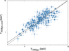 |
Fig. 4 Comparison between the true temperature measurements (from Table 5) and estimates from the scaling relations (from Table F.1). The dotted and solid lines show the 1:1 relation and the actual regression to the data respectively. |
5 Updated cluster statistics
With the current sample having twice as many C1 clusters as in XXL-100-GC (and 341 spectroscopically confirmed clusters in total), we are in a position to update a number of statistical results presented in the 2016 XXL release (a.k.a. DR1). Detailed analyses of these quantities in the current XXL-C1-GC sample will however be the subject of forthcoming papers. In this paper, we concentrate on a few basic properties of the XXL-C1-GC.
Regarding the 207 C1 clusters of XXL-C1-GC, only 191 are in pointings not affected by flares. All results involving the cluster selection function are therefore based on this subsample of 191 objects.
Five among these 191 clusters do not have a redshift determination and are therefore modelled using an incompleteness factor in the selection function. Excluding these five, the remaining sample of 186 clusters is used to compute the cluster luminosity function.
Eight out of these 186 clusters have no temperature measurement and their X-ray luminosity was estimated through scaling relations. This sample of 176 clusters is used to constrain the luminosity–temperature relation.
5.1 Redshift distribution and spectroscopic redshift sampling
The galaxy redshift sampling of clusters and the cluster redshift distributions are displayed in Figs. 5 and 6 for various cluster selections. Our total sample is the full list of clusters quoted in the present paper, including the few not yet spectroscopically confirmed clusters in Table G.2.
We see that the full list is very similar to the list of spectroscopically confirmed clusters, cf. top panel of Fig. 5. A Kolmogorov–Smirnov test shows no difference (at better than the 99.9% level) both for the redshift and the redshift sampling distributions. This figure also shows that, among the non-spectroscopically confirmed clusters, thirteen do not have any spectroscopic redshift, three of them have a single spectroscopic redshift (not the BCG), and one has two spectroscopic redshifts (the BCG being not available, spectroscopic confirmation is not validated either).
The XXL-N and XXL-S cluster samples are also similar in terms of redshift distribution (99.9% level for a Kolmogorov–Smirnov test). We however have on average more spectroscopically confirmed members (typically more than six spectroscopic redshifts) in the northern field compared to the southern field (see below for a more quantitative analysis of the cluster sampling). The probability of having similar samples is only at the 28% level with a Kolmogorov–Smirnov test.
C1, C2, and C3 cluster distributions are obviously different, as demonstrated by a Kolmogorov–Smirnov test. C2 and C3 clusters have lower spectroscopic sampling than C1 as these were not our primary spectroscopic targets. C3 mainly appears as a subpopulation of intermediate redshift clusters, with also a few distant (z ≥ 1) structures.
Finally,clusters brighter and fainter than the reference flux completeness limit of 1.3 × 10⁻¹⁴ erg s−1 cm−2 cover almost the same redshift range. Their redshift distribution is however different (probability of having similar samples only at the 53% level) with, not surprisingly, a lot more bright clusters at redshifts below 0.5. They also are very different (at the 98% level) in terms of spectroscopic sampling, the brightest clusters being better spectroscopically sampled.
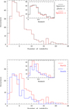 |
Fig. 5 Distribution of the number of spectroscopic redshifts inside clusters with a redshift measurement. The insets show the redshifthistograms of these samples. Top panel: spectroscopic + photometric redshift sample (black histograms), and spectroscopic redshift sample (red histograms) clusters. Bottom panel: XXL-N (red histograms) and XXL-S (blue histograms) clusters. Photometric redshifts are used in replacement of spectroscopic redshifts in these two histograms when spectroscopic redshifts are not available. |
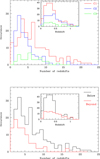 |
Fig. 6 Distribution of the number of spectroscopic redshifts inside clusters with a redshift estimate. The insets show the redshift histograms of these samples. Top panel: C1 (red histograms), C2 (blue histograms), and C3 (green histograms) clusters. Bottom panel: clusters with also a flux estimate fainter (black histograms) and brighter (red histograms) than the reference flux completeness limit of 1.3 × 10⁻¹⁴ erg s−1 cm−2. |
5.2 X-ray luminosities and fluxes
We display in Fig. 7 the distribution of cluster luminosities  (only when available through spectral fit, so C3 clusters are excluded) for the C1 and the C2 samples. In addition, Fig. 8 shows the cluster massM500,scal (derived from scaling relations) distribution for the same subsamples. We note that the cluster masses do not pertain here to direct spectral measurements (since temperatures are not available for the full sample) but were derived using scaling relations; we show these graphs to allow global comparisons with other cluster samples. In XXL Paper XIII, we mentioned the possibility that our total CFHTLS lensing masses were overestimated. Deep Subaru-HSC observations will provide higher signal to noise information and help us understand the contribution of non-thermal pressure in the total mass budget (Umetsu et al., in prep.).
Finally, in order to compare the C1 and C2 subsamples with the C3 subsample, we show in Fig. 9 the F60 (flux within a 60″ radius in the [0.5–2] keV band) distribution of the three subsamples. As expected, C1 clusters are brighter than the C2 clusters. C3 clusters pertain to two distinct populations as already stated in the previous section and showed in Adami et al. (2011). A large part of them are structures slightly fainter than the C2 clusters, and a few are bright and distant structures.
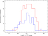 |
Fig. 7 X-ray luminosity ( |

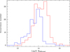 |
Fig. 8 Mass (in log units of M⊙) distributionof the clusters with a spectroscopic redshift estimate. Red histogram: the C1 sample; blue histogram: the C2 sample. The mass data points have been derived from scaling relations based on the cluster luminosities (cf. Sect. 4.3 and Appendix F). |
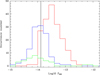 |
Fig. 9 X-ray flux (F60 in log unit of erg s−1 cm−2, within a 60″ radius in the [0.5–2] keV band) distribution for the clusters having a spectroscopic redshift. Red histogram: the C1 sample; blue histogram: the C2 sample; green histogram: the C3 sample. The black vertical line is the estimated reference flux completeness limit of 1.3 × 10⁻¹⁴ erg s−1 cm−2. |
5.3 Luminosity–temperature relation of the C1 sample
Figure 10 shows the XXL luminosity–temperature relation for the XXL-C1-GC sample (both parameters derived from spectral measurements). A fit to the data using a power law of the form
 (1)
(1)
was performed, where ALT, BLT, and γLT represent the normalisation, slope, and power of the evolution correction respectively. The power law was fit to the data, first using the BCES orthogonal regression in base ten log space (Akritas & Bershady 1996) assuming self-similar evolution (γLT = 1). The best fit parameters are given in Table 6. Comparing the XXL-C1-GC BCES fit to the XXL-100-GC fit, we find that the slope and normalisation are consistent.
We next fit the XXL-C1-GC scaling relation using the procedure outlined in XXL Paper III, taking fully into account the selection effects (we refer to Sects. 4.3 and 5.1 in XXL Paper III for specific details). However, the selection function was updated to match the current sample, instead of the XXL-100-GC selection function previously used. Figure 10 (upper panel) shows the XXL luminosity–temperature relation, with the best-fitting (bias-corrected) model given by the black solid line and the corresponding 1σ uncertainty shown by the grey shaded region. The best-fitting parameter values and their uncertainties are summarised by the mean and standard deviation of the posterior chains for each parameter from a Markov Chain Monte Carlo output. We used four parallel chains of 50 000 iterations each. To test for convergence, the stationary parts of the chains were compared using the Gelman & Rubin (1992) convergence diagnostic. The largest value of the 95% upper bound on the potential scale reduction factor was 1.02, indicating that the chains had converged.
The parameters of the luminosity–temperature scaling relation are given in Table 6, and illustrated with the scatterplot matrix in Fig. 11. We find that, within errors, the normalisation, slope, evolution and scatter (σLT) of the XXL-C1-GC luminosity–temperature relation agree with those of the XXL-100-GC sample. Figure 12 shows the comparison of the parameters with the XXL-C1-GC and XXL-100-GC samples. We find a lower normalisation than that found when using the BCES regression fit to the XXL-C1-GC sample (which did not account for selection biases), although the difference is minor, only weakly significant at the 1.7σ level.
Figure 10 (bottom panel) displays the evolution of the luminosity–temperature relation as inferred from our best-fitting model. The best-fit evolution is given by the black solid line along with the 1σ uncertainty, and the strong and weak self-similar expectations are given by the red and blue dashed lines, respectively. The best fit evolution is consistent with that found in XXL Paper III.
Large outliers in the luminosity–temperature relation were also inspected for possible AGN contamination. Initial visualisation of the X-ray images sometimes revealed point sources near the centre of the X-ray emission. These clusters where then removed from the sample to compute the luminosity–temperature relation. At present, a systematic search for possible contamination of all clusters has yet to be performed. However, this will be addressed with the release of the full XXL catalogue, where an improved pipeline will be used for joint cluster and AGN detection.
In order to test the effect of possible uncertainties on the mass temperature relation (cf. XXL Paper IV), we scaled down the normalisation of the XXL Paper IV mass temperature relation by 20%. We found that the luminosity–temperature relation parameters did not change significantly, as demonstrated in Fig. 13, showing the parameters contours using both the XXL Paper IV mass temperature relation and the scaled relation.
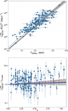 |
Fig. 10 Upper panel: luminosity–temperature relation with the best-fitting models. The light blue circles show the XXL-C1-GC clusters; the best-fitting model (including selection effects) is shown by the solid black line, the 1σ uncertainty represented by the grey shaded region. The best-fitting model fitted to the data using the BCES regression is shown as the dashed line. Bottom panel: evolution of the luminosity–temperature relation for XXL-C1-GC. The XXL-C1-GC clusters are represented by the light blue circles and the best-fitting model is given by the black solid line; the grey shaded region highlights the 1σ uncertainty.The “strong” and “weak” self-similar expectations are given by the red dashed and blue dashed lines, respectively. |
List of spectroscopically confirmed C1 and C2 clusters of galaxies.
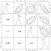 |
Fig. 11 Scatterplot matrix for the fit of the luminosity–temperature relation of the XXL-C1-GC sample. The posterior densities are shown along the diagonal; the 1σ, 2σ, and 3σ confidence contours for the pairs of parameters are shown in the upper right panels. The lower left panels show the Pearson’s correlation coefficient for the corresponding pair of parameters (text size is proportional to the correlation strength). |
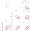 |
Fig. 12 Matrix plot comparing the 1σ, 2σ and 3σ contours for pairs of parameters of the luminosity–temperature relation, with the XXL-C1-GC and XXL-100-GC contours given by the black and red contours respectively. |
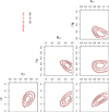 |
Fig. 13 Fit contours of the luminosity–temperature relation parameters using both the XXL Paper IV mass temperature relation (based on the XXL-C1-GC sample: black contours) and the scaled relation (normalisation of the mass–temperature decreased by 20% and using the same slope as in XXL Paper IV: red contours). |
5.4 X-ray luminosity function
Based on the new enlarged sample, we also revised our estimate of the cluster X-ray luminosity function from XXL Paper II. As for the luminosity–temperature relation, such a computation must rely on a complete subsample with measured selection function and therefore we focused on the XXL-C1-GC subsample. We relied on the available spectroscopic redshifts of Table 5 combined with the  ([0.5–2] keV band) resulting from the X-ray spectroscopic analysis (no estimates from scaling relations). For sixteen C1 clusters without a confirmed spectroscopic redshift, we used instead the tentative or photometric redshifts provided in Table G.2, while the five clusters without any redshift information are modelled using an incompleteness factor of 2.6%. This incompleteness is coming from the five C1 clusters (over 191) without a spectroscopic confirmation. During computation, we assume that these clusters are randomly selected among the full sample, and we then diminish the survey effective volume by the same factor of 2.6%. The mass and redshift distribution of these 2.6% is under-dominant compared to statistical errors. Finally, it was not possible to obtain the luminosity of eight clusters from X-ray spectroscopy, as the poor constraints on the temperature resulted in unphysical estimates of r500,MT and consequently unrealistically large or small extrapolation factors from the circular 300 kpc extraction region. For those eight clusters, we used instead the luminosity estimate based on scaling relations. This introduces a small level of inhomogeneity in our initial data set but we believe that the attached uncertainty is smaller than the effect of a large incompleteness. Indeed, higher redshift (fainter) clusters are more likely to be missing from our spectroscopically confirmed (X-ray spectroscopic) samples, which would distort the shape of the luminosity function.
From this sample, we estimated the luminosity function in our reference WMAP9 cosmology using the updated scaling relation model obtained in the previous section. The computation relied on the “cumulative effective volume correction” method introduced in Appendix B of XXL Paper II. This method is based on numerical derivation of a direct estimate of the cumulative luminosity, which has the advantage of reducing the Poisson noise by effectively relying on information from several luminosity bins to derive each value. This comes at the cost of a large bin-to-bin correlation but the tighter constraints on each bin remain unbiased.
The redshift averaged luminosity function for the whole sample is shown in the top panel of Fig. 14. Compared to our estimate of the luminosity function of XXL-100-GC in Paper II, the probed luminosity range only slightly increases while the errors are reduced by about 20%. However, the new luminosity function appears to be lower than the previous one, particularly at the low luminosity end where the discrepancy exceeds 3σ. These measurements are perfectly consistent between the two XXL subfields, as illustrated by the bottom panel of Fig. 14, effectively excluding a number of possible systematic errors in the modelling of the selection function like the dependence on absorption, depth or pointing layout. To further investigate the origin of the discrepancy, we also computed the luminosity function based on the old luminosity–temperature relation of XXL Paper III (blue dot-dashed line in Fig. 14) which revealed that the tension originates from the change both in the number of detected sources per luminosity and redshift bin in the new sample, and in the effective volumes computed for different scaling relation models. With the old model, the tension between XXL-C1-GC and XXL-100-GC would mostly be lower than 2σ (even at the low luminosity end where it just reaches 2σ). In other words, when using the old model for computing the luminosity–temperature relation, all the discrepancy can be understood in terms of cosmic variance. If we compare the differences between red and blue curves of Fig. 14 (upper figure) with statistical uncertainties and north versus south variations, the observed differences are not significant.
We also investigated the redshift evolution of the luminosity function by splitting the sample into three redshift bins containing approximatively the same number of clusters. As shown in Fig. 15, there is no evidence for evolution below z ~ 0.43 while a significant negative evolution is observed at z > 0.4. This result is fully consistent with expectations calculated using the WMAP9 cosmological model and our preferred set of scaling relations. The absence of evolution below z ~ 0.4 also rules out different redshift weights as the origin of the lower luminosity function compared to XXL-100-GC, since all the constraints at low luminosity come from low redshift clusters.
The measured values (both redshift averaged and in redshift bins) are provided in Tables 7 and 8 for the differential and cumulative luminosity functions. We however stress that our effective volume correction method might slightly bias the cumulative distribution at low luminosities, as it relies on the full shape of the modelled WMAP9 luminosity function to weight the luminosity dependent effective volume.
Clusters affected by AGNs represent < ~5% of the full C1 sample and were not removed from the calculation of the luminosity function. This allows a direct comparison with the preliminary results of XXL Paper II.
We also tried to estimate how many clusters in the X-ray luminosity function could be affected by cluster-cluster X-ray blending, potentially leading to the loss of some faint clusters and the artificial addition of bright clusters. None of the cluster pairs or super-clusters listed in Tables E.1 and 9 are contributing to this bias as they are detected as independent clusters. However, the line-of-sight superpositions and X-ray blends, listed in Appendix B, can affect the X-ray luminosity function. This is the case for the line of sight of XLSSC 041 where a z = 0.557 cluster is missed, of XLSSC 539 including two clusters at z = 0.169 and 0.184, of XLSSC 096 with two clusters at z = 0.203 and 0.520, of XLSSC 151 with two clusters at z = 0.189 and 0.280, of XLSSC 044 with two clusters at z = 0.263 and 0.317, and of XLSSC 079 with two clusters at z = 0.19 and probably at ~0.52. This represents however <5% of the sample used to compute the X-ray luminosity function and the effect is therefore probably negligible.
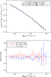 |
Fig. 14 Upper panel: X-ray luminosity function ([0.5–2] keV band) of the C1 cluster sample based on the 186 C1 clusters in good pointings and with redshift information. The calculation is averaged over the whole survey volume (z in 0.0–1.3) and includes an incompleteness factor of 2.6% for the five C1 clusters without any redshift estimate. The method is the same as in XXL Paper II. For comparison, the luminosity function of the XXL brightest 100 cluster sample (XXL-100-GC) is shown with the red dashed line. Finally, the dot-dashedblue line indicates the luminosity function of the C1 sample recomputed for with the old LX − T relation of XXL Paper III, as was assumed for the XXL-100-GC sample. Lower panel: residuals of the C1 luminosity functions computed from only the northern or southern XXL field with respect to the complete luminosity function shown in the upper panel. |
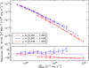 |
Fig. 15 Redshift evolution of the C1 X-ray luminosity function. The calculation relies on the same assumptions as for the full survey volume luminosity function of Fig. 14, but the sample is split into three redshift bins containing approximately the same number counts of clusters. The dashed lines show, for the same redshift bins, the luminosity function expected in the WMAP9 cosmology from our scaling relation model (M500,WL − T300 kpc
from XXL Paper IV and |
Tabulated values of the differential luminosity ([0.5–2] keV) function for the C1 sample.
Tabulated values of the cumulative luminosity ([0.5–2] keV) function for the C1 sample.
6 Witnessing the evolution of massive structures: from super-clusters to fully collapsed fossil groups
In order to illustrate the large variety of objects detected in the XXL Survey, we will follow in this section the history from what could be theprogenitors of very massive clusters (super-clusters), to merging clusters in an already advanced stage (e.g. XLSSC 110), and tothe possible final stage of group of galaxies (fossil groups).
To give a general flavour of the structures present in the XXL Survey, we also present in Appendix B the notable cluster superpositions we detected, and the most distant cluster in our survey (XLSSC 122, cf. Mantz et al. 2014, hereafter XXL Paper V) along with additional spectroscopic follow-up of this cluster.
6.1 Super-clusters
We search for a-priori physical associations between individual clusters of galaxies. We will arbitrarily call “super-clusters” the associations of at least three clusters (whatever their separation). Cluster pairs (association of only two clusters) are not considered as super-clusters.
6.1.1 Friends-of-friends detected super-clusters
We used all spectroscopically confirmed C1, C2, and C3 clusters to search for super-clusters in the two XXL fields. The analysis was restricted to the [0.03–1.00] redshift range.
We first performed a classical three-dimensional friends-of-friends analysis (FoF hereafter) to estimate the critical linking length, ℓc, for each field, the one that maximises the number of super-clusters (for instance Eckert et al. 2016). We found, respectively for XXL-N and XXL-S, 27 and 29  Mpc. While a FoF analysis with this linking length would be ideal if the sample was relatively homogeneously distributed in z. In the real world, we need a weighting function to weight ℓc.
We measured the cluster space densities by dividing the cluster sample in ten bins of redshift and calculating the respective cosmological volumes. The density falls roughly exponentially from z ~ 0.03 up to z ~ 0.7, then follows a plateau and, finally, the last bin is very undersampled. Since this density distribution can be considered as the inverse of the selection function, we could use it to weight ℓc with redshift. We used the pure exponential fit (cf. Eq. (3)), to bins between 0.22 ≤ z ≤ 0.71, which reproduces very closely the exponential plus plateau behaviour.
Thus, we applied a “tunable” FoF, as for example in Chow-Martínez et al. (2014), to the sample by using an exponential fit in order to weight the ℓc and compute the local linking length, ℓ(z), for each targeted cluster. We have
![Mathematical equation: \begin{equation*}\ell(z) = \left[ \frac{3}{4 \pi \, { d}(z)} \right]^{1/3} \, \ell_c , \end{equation*}](/articles/aa/full_html/2018/12/aa31606-17/aa31606-17-eq8.png) (2)
(2)
where
 (3)
(3)
is the normalised density (weighting) function.
We found 21 super-clusters in the XXL-N field data and 14 in XXL-S, considering only super-cluster candidates with a multiplicity (number of member clusters) greater than or equal to 3 (cf. Table 9). We adopted the internal denomination XLSSsC for XXL super-clusters (replacing the preliminary notation used in XXL Papers II and XII) to avoid any confusion with regular individual clusters. The centres of the super-clusters were calculated as the geometrical centre of the member clusters. Super-clusters described in the present paper have sizes up to 60 Mpc, and this is around the median value for the largest superclusters in the local Universe (e.g. Chow-Martínez et al. 2014).
We also give (in Appendix E) in Table E.1 the list of cluster pairs (16 in the XXL-N field data and 23 in the XXL-S) detected with the same FoF approach.
The use of a tunable linking length made it possible to detect super-cluster candidates even at z ≥ 0.6, where the completeness of the sample becomes critically low. The algorithm supposes that there is an “additional density” at such redshifts that maintains a mean density more or less similar to that of nearby clusters. Of course this virtual density may be or not connecting the clusters to form super-clusters. In practice, the linking length becomes larger and the possibility of having “connected” clusters by chance is higher. Thus, we have to take these high-redshift super-clusters with caution. At z ~ 0.8 (the most distant super-cluster in the present paper is detected at this redshift), the linking length is ~80 Mpc, which is typically of the same order as the largest known super-clusters (e.g. Horologium-Reticulum, Fleenor et al. 2005, or the BOSS Great Wall, Lietzen et al. 2016).
List of detected super-cluster candidates with the FoF approach.
6.1.2 Voronoi tessellation detected super-clusters
We applied a 3D Voronoi tessellation (e.g. Icke & van de Weygaert 1987; Söchting et al. 2012), to the data in the two XXL fields in order to assess the reliability of the structures previously found. Voronoi tessellation was not used to directly detect super-clusters. It is a partitioning of a volume according to the distribution of objects inside this volume. In the first step, we divided each cone volume into a number of optimum polyhedra equal to the number of clusters in that volume (Voronoi cells). If the clusters are distributed with no sampling variation with redshift, the inverse of the Voronoi cell volume represents directly the local density at the cluster positions. In our case, the sampling is not constant with redshift because at high redshift the linking length becomes larger than the typical cluster-cluster separation. The next step was then to correct the Voronoi cells volume by applying the weighting function already applied to the linking length in the FoF analysis, in order to compensate for the undersampling at the highest redshifts. The condition here was to adjust the distribution of volumes maintaining the total volume fixed (and, so, the mean volume or, equivalently,the mean density). The local density for each cluster can be obtained directly from the inverse of its Voronoi cell volume.
Then we applied a threshold above which the local densities of the clusters are at least twice the mean density (i.e. a density contrast of 1). By counting the number of “overdense” clusters over the number of member clusters in each super-cluster (detected by FoF) we could determine a “reliability index” R in such a way that:
-
R = 1 represents super-clusters with 25% or less of the member clusters in the overdense category;
-
R = 2 with a fraction between 26 and 50%;
-
R = 3 with a fraction between 51 and 75%;
-
R = 4 with more than 75% of the clusters in the overdense category according to the Voronoi analysis.
We compared our super-cluster list with the one of XXL Paper II also drawn from the XXL cluster sample but with a different method and with a more limited individual cluster sample (only the 100 XXL brightest ones). The five XXL Paper II and the one Paper XII super-clusters are all redetected in the present paper. We confirm them at very similar redshifts and we sometimes add more member clusters. The only noticeable exception is XLSSsC N08 for which three clusters were associated with the supercluster XLSSsC N03 which was not detected in XXL Paper II when the number of XXL spectroscopically confirmed clusters was lower. Melnyk et al. (2018, hereafter XXL Paper XXI) also found that the most populated agglomerates of AGNs are associated with some of the superclusters listed in Table 9.
6.2 Merging process: the peculiar case of the XLSSC 110 system
In this section we present an example of a merging system for which we collected additional data allowing us to examine the structure in more depth. The XLSSC 110 system is one of the most complex compact confirmed C1 clusters (z = 0.445) we detected within the XXL Survey. Initially confirmed with six spectroscopic redshifts, this structure shows a peculiar behaviour, with three apparent BCGs very close in redshift. The X-ray emission coming from this structure is also not equally distributed over the galaxy distribution. The BCG associated with the main X-ray peak is possibly undergoing a rather rare triple merging. This led us to collect more spectroscopic data for this structure and we got PMAS (PPak mode) integral field observations for this purpose at the 3.5 m Calar Alto telescope in 2015 and 2016. We describe the data collection in Appendix C.
Discussion
The final list of obtained redshifts is given in Table 10. We confirm the value of three previously measured redshifts and successfully measure five new redshifts. Among these new redshifts, four are located in XLSSC 110. This structure is clearly dominated by four bright galaxies. Two of them (ids 1 and 2) seem located at the bottom of the potential well, as traced by the X-ray contours in Fig. 16, while the other two (ids 4 and 3) are located to the cluster north.
With redshifts in Table 10, and only considering the secure spectroscopic redshifts (flags greater than or equal to 2, considering the new measurements when available), we have the minimal number of redshifts to search for possible substructures inside XLSSC 110 with the Serna & Gerbal (1996, hereafter SG) technique. Already used in several articles (e.g. Adami et al. 2016, hereafter XXL Paper VIII), this hierarchical method first identifies the substructures in a dynamically linked galaxy population, and also provides rough estimates for the mass of the substructures. We note that masses are estimated through a basic version of the Virial theorem (cf.Guennou et al. 2014). More precisely, the SG hierarchical method calculates the potential binding energy between pairs of galaxies and detects substructures by taking positions, magnitudes, and redshifts into account.
The SG method detects three substructures in the XLSSC 110 cluster. The first substructure has six galaxies and an estimated optical dynamical mass of (1 ) × 1013 M⊙ (green circles in Fig. 16). It can be considered as the cluster original structure. Within this structure, the more linked galaxies are #1 and 2, then 5, and then 6, 10, and 8. Galaxy #8 is clearly a disk galaxy, is the one with the largest redshift, and is probably in an infalling process onto the main structure.
Two other substructures are detected. They are smaller (2 galaxies each: red and white circles in Fig. 16). Their levels of binding energy to the main structure are different. The red structure of Fig. 16 is more linked to the main green structure than the white one. In physical terms, this could mean that the red structure has been in the process of merging with the main structure for a longer time than the white one. Considering the green and red structures together, the estimated optical dynamical mass is 3 × 10¹³ M⊙.
This behaviour is in good agreement with our initial visual interpretation of the physics of this cluster. We note, however, that our redshift catalogue remains quite sparse and more spectroscopic redshifts would be required to confirm this interpretation.
Results of the redshift measurements on the detected galaxies in the PMAS/PPak data for XLSSC 110 cluster.
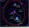 |
Fig. 16 CFHTLS 2.4′× 2.3′ i′ image of XLSSC 110 with known galaxy members of the structure. Green circles are from the main dynamical structure, and red and white circles are from two secondary structures following the Serna–Gerbal technique. The large red circle represents a 500 kpc radius. White contours are for the X-ray emission. The given numbers are the galaxy identification in Table 10 and the redshifts of the same table (giving priority to the new redshifts we measured ourselves). |
6.3 Fossil groups
Fossil groups (FG hereafter) are peculiar structures of galaxies with an extended X-ray halo. Jones et al. (2003) defined them more precisely as structures with an X-ray bolometric luminosity of more than 1042 erg s−1 and a difference of two magnitudes or more between the first and second ranked galaxies within half the group Virial radius. These structures mostly appear in the optical as isolated large early type galaxies. Most of the time, only X-ray data can reveal the existing extended massive halo. Several other studies were made as in Khosroshahi et al. (2007) where additional criteria were added. Sometimes studied individually (e.g. Adami et al. 2007, 2012 or Ulmer et al. 2005), FGs were also the subject of statistical studies: for example the FOGO sample (Santos et al. 2007; Girardi et al. 2014).
6.3.1 Our selection
Most of the studies to date, were based on optically selected FG samples (e.g. the FOGO sample). We propose here a first catalogue of candidates based on an pure X-ray selection. We decided not to limit our sample to a specific X-ray luminosity range. We therefore explored the full XXL spectroscopically confirmed cluster luminosity range. For each of the spectroscopically confirmed galaxy structures, we examined their optical counterparts both in photometry (using photometric redshift techniques) and in spectroscopy (with the XXL spectroscopic general follow-up) to search for FG candidates. We used a slightly different radius criterion: instead of 0.5 ×r200, we used 1 ×r500,scal (from Table F.1). Following Roussel et al. (2000), the ratio between r500,scal and r200 is 0.66. Our criterion is therefore slightly more stringent than the one of Jones et al. (2003).
We first selected all the spectroscopically confirmed galaxy structures in our sample. Then we used our photometric catalogues giving the position and magnitudes of objects in the fields, their photometric redshift, and the associated redshift probability distribution function (PDF hereafter). A spectral star galaxy separation is also available.
We selected for each structure in a r500,scal radius all objects with a high probability to be a galaxy (probability to be a star lower than 10%). When available, we added the spectroscopic redshift to this sample from our spectroscopic database6, only considering spectroscopic redshifts measured with more than ~85% confidence (i.e. spectroscopic flags two or better, e.g. Le Fèvre et al. 2013).
At this step, we selected the dominant galaxy, defined as the brightest galaxy in the r′ band at <75 kpc from the X-ray centre. This distance is approximately the maximal distance we can expect in a cluster between the BCG and the bottom of the potential well (e.g. Adami & Ulmer 2000).
If by chance this galaxy has a spectroscopic redshift, we check if the redshift is consistent with the structure redshift. The consistency criterion is defined as ±3 times the velocity dispersion of the structure estimated from X-ray luminosity (giving priority to direct spectral measurements). If not consistent, this galaxy is removed and the next brighter galaxy is considered.
If no spectroscopic redshift is available, we consider the photometric redshift instead, exceptionally enlarging the consistency criterion to ±0.1 in redshift to take into account of the larger uncertainty of the photometric redshifts (±0.056 in the south and ±0.034 in the north, Fotopoulou et al. 2016 hereafter XXL Paper VI, see below) compared to the spectroscopic ones.
The dominant galaxy being defined, we selected all galaxies along the structure line of sight (within r500,scal) in the next two-magnitude interval (this requires obviously the magnitudes to be successfully measured). These candidate lists were finally scrutinised to conclude about the fossil group nature of the considered structures. For a considered structure and a given galaxy, we computed the probability for this galaxy to be outside of the previous ±3 times velocity dispersion interval.
-
For the galaxies with a spectroscopic redshift, the galaxy probability is 1 (not FG member) or 0 (FG member) depending on the redshift and the structure velocity dispersion.
-
For the galaxies without a spectroscopic redshift, the probability is computed with the PDF of the galaxy, simply integrating it out of the structure redshift interval.
Taking the product of these probabilities for the different galaxies in the candidate list (excluding the BCG) to be FG members or not, this gives finally the probability for the structure itself to be a fossil group. As an example, if a structure has a single galaxy within the two-magnitude range fainter than the BCG (besides the BCG itself) with a spectroscopic redshift within the redshift interval, the probability for this structure to be a fossil group will be null.
Each of our confirmed galaxy structures was then scrutinised taking into account their probability to be a FG. After having removed obvious interlopers (e.g. structures polluted by bright stars, complex structure superpositions, incomplete photometric samples), we decided to retain as FG possible candidates only structures with a probability >20% to be a FG. This level was determined a priori as the minimum percentage level below which all structures were easily classified by hand as non-FG structures. This level is intentionally low and it will imply a large number of false-positives. FG being however rare objects, it is a way to not lose any of them. These potential candidates are given in Table 11.
List of FG candidates.
6.3.2 Properties of our FG candidates
We can ask the question of why 2.6 times more FG “candidates” (5 times more if we consider only the high probability FGs) are found in thesouthern XXL field than in the northern field.
First, an obvious explanation could be the spectroscopic follow-up sampling which is much higher in the north thanks to the SDSS, GAMA, VIPERS, and VVDS surveys. To exclude a given galaxy structure from the FG class, we need to be sure that a galaxy is inside the structure with a magnitude fainter than the BCG by <2 magnitudes. Let us assume the existence of such a galaxy. The uncertainty on its redshift location with regard to the structure’s mean redshift is typically the redshift measurement uncertainty.
If the redshift is spectroscopic, we will know quite precisely where the galaxy is and the probability to (wrongly) estimatethat the galaxy is outside the structure will be low. The structure will therefore be excluded from the FG class with a high probability;
If the redshift is photometric, the probability to (wrongly) estimate that the galaxy is outside the structure will be muchhigher (photometric redshift uncertainties are typically at least twenty times larger than for spectroscopic redshifts). The structure may therefore not be excluded from the FG class.
It is therefore much easier to exclude a structure from the FG class with spectroscopic redshifts than with only photometricredshifts. In our data, statistically, a northern galaxy structure line of sight is sampled by ~17 times more redshifts than a southern line of sight. This may indeed favour the existence of a larger number of remaining FG candidates in the southern fields. However, we note that in terms of galaxy structure spectroscopic members, northern structures are not significantly better sampled than southern structures.
Second, the photometric redshifts are less precise in the south (uncertainty of 0.056 in redshift and catastrophic error percentage of 15%) than in the north field (uncertainty of 0.034 in redshift and catastrophic error percentage of 3%), Fotopoulou et al. (priv. comm.). These numbers will be described in a future XXL Paper, but the catastrophic error percentage can induce non negligible uncertainties on the probability of a structure to be a FGs (cf. Appendix A for a complete description of the computation). Taking these uncertainties into account (cf. Table 11), basically none of the northern FG candidates are affected, while up to four southern FG candidates may not be real FGs. The previously quoted ratio between northern and southern FG candidates would only be 1.8 with just this explanation. This does not, however, explain the 1:5 ratio between the number of high probability FG candidates in the two fields, as none of these objects are affected.
Another way to test if we have significantly more FG candidates in the southern than in the northern area is simply to sum the probability of all massive structures (not only the FG candidates listed in Table 11) in both fields of being such FGs. If the two fields are similar from a cosmic variance point of view, these sums should be identical. We find a ratio of 1.1 between the two sums, speaking in favour of the northern and southern fields being indeed similar.
We also compared (using a bi-dimensional Kolmogorov–Smirnov test) the distribution of the northern and southern FG candidates within the X-ray luminosity vs X-ray luminosity uncertainty space, and within the X-ray luminosity vs redshift space. X-ray luminosity is here estimated from scaling laws. In the first case, the probability to have similar distributions in the north and in the south is more than 65%. In the second case, the probability to have similar distributions is >99%.
We however stress that only a spectroscopic follow-up of the photometric redshift classified galaxies will definitely tell us whether we have a significant difference between the FG density in the northern and southern XXL fields, in particular when considering high probability FG candidates. This is also the only way to assess nominatively the FG nature of our candidates. We show in Table 11 and in Fig. 17 that the uncertainty of a candidate to be a FG is obviously related to the spectroscopic redshift sampling percentage for the considered line of sight (within the two-magnitude range and BCG excluded). The fewer spectroscopic redshifts we have along the line of sight, the more photometric redshifts we need and they are potentially affected by catastrophic errors. Reaching a sampling percentage of better than 30% would lead to a negligible uncertainty on the FG nature due to photometric redshift catastrophic errors. The inset in the same figure also shows that the magnitude range of the lacking spectroscopic redshifts (within the two-magnitude range) is easily reachable with an integral field spectrograph such as MUSE/VLT.
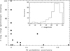 |
Fig. 17 Percentage of spectroscopic redshifts within r500,scal that are found in the two-magnitude interval fainter than the BCG, as a function of the uncertainty on the probability for a cluster to be a fossil group (given in Table 11). Inset: r′ band magnitude histogram of the galaxies without a spectroscopic redshift, and within the two-magnitude range of our FG candidates. |
6.3.3 Are our FG candidates different from the general XXL cluster population?
We cannot reproduce the same tests as in the previously quoted literature studies without performing additional spectroscopical follow-up of our FG candidates. We can however perform a basic test: are our FG candidates simply extreme cases of the general galaxy structure population, obeying to the same formation process, evolution path, etc.? Or alternatively, are FGs an independentpopulation of galaxy structures? Several studies as Girardi et al. (2014), Zarattini et al. (2014) and Kundert et al. (2015) seem to show that FGs behave very similarly to normal galaxy structures. Taking into account the full spectroscopically confirmed cluster sample in the XXL northern area (the one which has the best spectroscopic sampling), we computed the number of magnitudes we can add to the brightest cluster member r′ magnitude (as defined previously for the FGs) in order to achieve a probability >20% to have no galaxy within the defined magnitude interval. Good FG candidates therefore appear in this plot as the galaxy structures with the largest magnitude gaps, greater or equal to 2. In Fig. 18, there appears to be a continuous variation of this gap, the good FG candidates being only the extreme cases. The same exercise in the XXL southern area gives very similar results. These histograms may be however polluted by interlopers (galaxies with photometric redshifts, but outside of the cluster if we had a spectroscopic redshift). Once again, this shows that a more complete spectroscopic redshift follow-up is needed for these FG candidates. This also speaks in favour of a common origin between regular groups of galaxies and FGs.
FG candidates are however significantly fainter in terms of X-ray luminosity compared to the global cluster sample. A Kolmogorov–Smirnov test shows that there are <4% of chances that the global sample of clusters has a similar X-ray luminosity (estimated from scaling laws) distribution compared to the luminosity distribution of our FG candidates.
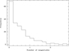 |
Fig. 18 Histogram of the number of magnitudes we can add to the brightest cluster member r′ magnitude in order to achieve a probability larger than 20% to have no galaxy within the defined magnitude interval (for all the spectroscopically confirmed clusters of the XXL northern area). |
7 Conclusion
In the present paper we released several catalogues based on a sample containing 365 clusters in total. We described the follow-up observations, the precision of the measured galaxy redshifts, and explained the procedure adopted to validate the cluster’s spectroscopic redshifts.
We provided X-ray flux, luminosity, temperature, and direct gas mass measurements for a large part of the sample extending from z; ~ 0 to z ~ 1.2 (with a cluster at z ~ 2). We also estimated from scaling relations luminosities, temperatures, and total masses. Using this 365 cluster sample, we updated the previous XXL luminosity function and luminosity–temperature relations only based on the 100 brightest clusters. We presented an enlarged catalogue of super-clusters and a sample of 18 fossil group candidates.
This intermediate publication is the last before the final release of the complete XXL cluster catalogue. It provides a unique inventory of medium-mass clusters over a 50 deg2 in a 0 < z < 1.2 cone and gives a flavour of the general properties of the cluster sample.
Acknowledgements
The authors thank the referee for useful comments. XXL is an international project based around an XMM-Newton Very Large Programme surveying two 25 deg2 extragalactic fields at a depth of ~5 × 10⁻¹⁵ erg cm−2 s−1 in the [0.5–2] keV band for point-like sources. The XXL website is http://irfu.cea.fr/xxl. Multiband information and spectroscopic follow-up of the X-ray sources are obtained through a number of survey programmes, summarised at http://xxlmultiwave.pbworks.com/. The Saclay group acknowledges long-term support from the Centre National d’Études Spatiales (CNES). EK thanks CNES and CNRS for support of post-doctoral research. We also acknowledge financial support from “ProgrammeNational de Cosmologie et Galaxies” (PNCG) of CNRS/INSU, France. We also thank Calar Alto Observatory for allocation ofdirector’s discretionary time to this programme. C.A.C. acknowledges financial support from CONACyT (Mexico) for sabbatical leave and Laboratoire d’Astrophysique de Marseille for hospitality and support during stay. Also based in part on data acquired through the Australian Astronomical Observatory, under programme A/2016B/107. We also thank the whole GAMA and VIPERS teams for sharing unpublished data. DR is supported by a NASA Postdoctoral Program Senior Fellowship at the NASA Ames Research Center, administered by the Universities Space Research Association under contract with NASA. MP acknowledges the financial support from Labex OCEVU (ANR-11-LABX-0060). FP and MERC acknowledge support by the German Aerospace Agency (DLR) with funds from the Ministry of Economy and Technology (BMWi) through grant 50 OR 1514 and grant 50 OR 1608. SA acknowledges a post-doctoral fellowship from TUBITAK-BIDEB through 2219 program. SF acknowledges support from the Swiss National Science Foundation.
Appendix A: Uncertainty on the probability of an XXL structure to be a FG
In the process of computing the probability of an XXL structure to be a FG, galaxy photometric redshift uncertainties are probably not crucial in our case because we are directly using the spectral energy distributions. A high catastrophic error percentage can however have a non negligible effect as it can be the sign of a failed computation of the spectral energy distribution itself. Assuming this is the case, we computed for each of our FG candidates the number N of galaxies potentially affected. This number N is the total number of galaxies along the considered FG line of sight within the two-magnitude range, minus the number of galaxies with a spectroscopic redshift (these ones are not affected by the catastrophic errors). For each of these galaxies, the redshift is therefore unknown. The probability to be outside of the considered structure is then equal to the ratio of the explored redshift range (z = [0–6]) over the typical redshift range covered by a massive structure (<0.024). This gives a statistical probability to be outside of the considered structure of 99.6% if we assume that no redshift selection effects are at play. For each of the FG candidates, we therefore simulated 100 times the replacement by 99.6% of the initially computed structure membership probability of the N galaxies. This gave us an estimate of the uncertainty of the considered massive structures of being FGs (cf. Table 11).
Appendix B: Notable superpositions
In this section we present noticeable line of sight cluster–cluster associations (most with overlapping X-ray emissions). This is not a systematic search in the XXL Survey, but just a summary of the evident associations we eyeballed in the survey. A list of potential cluster pairs is given in Table E.1. All images are CFHTLS i′ band images, with north to the top and east to the left. The white contours are the XMM X-ray contours, which were created using local minimum and maximum and a logarithmic scale with ten levels.
XLSSC 035: this structure is a C1 confirmed cluster. It presents a nice superposition of a z ~ 0.174 cluster and of a bright galaxy at z = 0.0691 (cf. Fig. B.1). Initially, this structure was classified at the redshift of this bright galaxy (assumed to be the BCG of the cluster). Later redshift measurements showed that the structure thought likely to be associated with the X-ray extended emission is in fact more distant. A second measure of the bright galaxy was made, confirming its z = 0.0691 redshift.
 |
Fig. B.1 CFHTLS i′ band 4.5′× 3′ image around the XLSSC 035 confirmed z = 0.174 cluster. Green circles represent the member galaxies plus the bright foreground galaxy discussed in the text. White contours arefor the X-ray emission. |
XLSSC041: this structure is a very regular C1 cluster at z = 0.142. Figure B.2 however shows another X-ray concentration at the (36.3682, −4.2602) coordinates towards the south-west. This secondary peak nicely corresponds to a concentration of four galaxies at a mean redshift of 0.557. XLSSC 041 therefore seems to be a regular cluster polluted by another line of sight z = 0.557 cluster.
 |
Fig. B.2 CFHTLS i′ band 5.5′× 3.5′ image around the XLSSC 041 confirmed z = 0.142 cluster. Magenta circles represent the member galaxies. White circles are the galaxy members of the background cluster at z = 0.557. White contours are for the X-ray emission. |
XLSSC 514 and XLSSC 515: these two clusters are confirmed C1 structures and are very close in projection. Their X-ray emissions are merged on the sky, the first one being at z = 0.101 and the second one at z = 0.169 (cf. Fig. B.3).
 |
Fig. B.3 CFHTLS i′ band 4.5′× 3′ image around XLSSC 514 and XLSSC 515 confirmed z = 0.101 and 0.169 clusters. Magenta circles represent the member galaxies of the two clusters. Figures are showing the central areas of these structures. White contours are for the X-ray emission. |
XLSSC 539: this C1 cluster has two components as shown in Fig. B.4. The first one at z = 0.184 was assumed as the main cluster redshift because very well correlated with the X-ray peak. Another cluster at z = 0.169 is also present towards the east and is probably an infalling structure entering a future merging state.
 |
Fig. B.4 CFHTLS i′ band 7.5′× 5′ image around XLSSC 539 confirmed z = 0.184 and 0.169 double structure. Red circles represent the member galaxies of the two components. We clearly see the central z = 0.184 structure and the other component at z = 0.169 towards the east. The large red circle represents a 500 kpc radius area. White contours are for the X-ray emission. |
XLSSC 096: this X-ray source is a very nice example of close superposition on the sky of two different galaxy structures (cf. Fig. B.5). The first one is sampled with six redshifts at z = 0.520 (including a BCG-like galaxy at z= 0.5206). The second one is exactly on the same line of sight, at z = 0.203 (sampled by two spectroscopic redshifts, including also a BCG-like galaxy). We choose to adopt z = 0.520 because of the greater richness of this component.
 |
Fig. B.5 CFHTLS i′ band 4′ × 2.5′ image around XLSSC 096. Green squares represent the member galaxies of the main structure at z = 0.520 and magentacircles are the foreground structure at z = 0.203. The large red circle represents a 500 kpc radius area. White contours are for the X-ray emission. |
XLSSC 151: this cluster is also a noticeable superposition. The main structure is at z = 0.189, clearly located on the main X-ray peak (cf. Fig. B.6). However, another structure also appears at z = 0.280, dominated by a BCG-like galaxy which also may be correlated with a secondary X-ray peak.
 |
Fig. B.6 CFHTLS i′ band 6.5′× 4.5′ image around XLSSC 151. Magenta circles represent the member galaxies of the main structure at z = 0.189 and blue circles those of the background structure at z = 0.280. The large red circle represents a 500 kpc radius area. White contours are for the X-ray emission. |
XLSSC 044: this line of sight is complex with two richly sampled structures on it (cf. Fig. B.7). The main one at z = 0.263 has nineteen known members and the other one at z = 0.317 has ten known members.
 |
Fig. B.7 CFHTLS i′ band 6.5′× 4.5′ images of two superposed structures. Magenta circles represent the member galaxies of the two structures at z = 0.263 (upper panel) and at z = 0.317 (bottom panel). The large red circle represents a 500 kpc radius area. White contours are for the X-ray emission. |
We alsonote than XLSSC 149 and 150 (cf. Fig. B.8) are two clusters with non overlapping X-ray emission (at the depth of the XXL observations). They have however exactly the same redshift (z = 0.292) and are separated by <500 kpc. This means that we deal with two low mass structures (each at temperature of ~2 keV) with the potential to merge in the future. This is supported by the fact that they are both part of the N01 super-cluster (cf. Table 9).
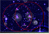 |
Fig. B.8 CFHTLS i′ band 6.5′× 4.5′ image of the XLSSC 149 and 150 structures. Magenta circles represent the member galaxies of the two structures at z = 0.292. The large red circles represent 500 kpc radius areas. White contours are for the X-ray emission. |
XLSSC 079: this cluster may suffer from a superposition effect. The main structure is clearly detected at z ~ 0.19. However, another structure may be present on the same line of sight at z ~ 0.52. An SDSS galaxy spectroscopic redshift is available at z = 0.5171 (α = 34.49248, δ = −4.86538) in the DR12, very close to the main structure. This is not enough to officially confirm this superposition, but this value may support the detection of two literature clusters detected at the same place on a photometric redshift basis: CFHT-W CL J021757.8-045142 (Wen et al. 2012) at z = 0.537 and SXDF35XGG (Finoguenov et al. 2010) at z = 0.46.
Appendix C: IFU observations of XLSSC 110
The observed field was centred on the cluster position. The PPak-IFU of PMAS at the 3.5 m Calar Alto telescope is an hexagonal packed fibre-bundle instrument with 331 object, 36 sky and 15 calibration fibres (2.68″ diameter each, separated by 3.57″ and 3.12″, respectively in the x and y coordinates, resulting in a 60% filling factor), covering a projected FOV in the sky of 74″ × 65″.
Twelve 1200 s exposures were obtained during two observing runs (2015, December 31 and 2016, February 01–02), with two pointings to each of the six positions (Table C.1) in a dithering mode, using the V300 grating and 4 k × 4 k (15 μm pixels, 2.57–2.88 read out noise and 1.14–1.29 e−1/ADU) CCD.
Details of the PMAS/PPak observations of XLSSC 110: exposure number, run date, coordinates (J2000), air mass range.
Calibration images consisted of one set of ten bias (0 s exposures) for each observing run, five and twelve twilight sky flats (1–30 s), respectively, plus continuum dome-flat fields (5 s) and HgHe calibration arc lamps (60–120 s) via fibres for every science image. Darkframe exposures were not taken since the instrument is regularly checked and there is no dark current currently. Standard stars (BD +25 4655, G191B2B and BD +33 2642) and a comparison elliptical (NGC 499) were also observed during the observing runs.
The spectral images are read separately in four CCD blocks (a, b, c and d quadrants, from bottom-left anti-clockwise), reduced together with the P3D software (cf. Sandin et al. 2010). Data reduction followed standard steps for IFS: bias combinationand subtraction, detection of spectra along the cross-dispersion axis, their tracing along dispersion axis, extraction, transmission correction, cosmic ray events removal and wavelength calibration. The resulted calibrated spectra cover approximately 3862 Å (ranging from 3749 to 7610 Å) with a linear dispersion of about 1.92 Å/pixel (or ~100 km s−1 per pixel at 5700 Å). Differential atmospheric refraction correction was not applied. Sky fibres were averaged for each image, excluding some (1 spaxel in the first run and 3 in the second) with inconsistent signal, to prepare master sky spectra which were subtracted from all the spaxels of that image.
Thus, the brightest objects in the field of each position of the dithering pattern (6) were first identified individually to have the spectra of the respective spaxels clipped and, after, summed. One of the dithering positions (the middle one of the second run) was not used due to very low S/N. Fifteen objects were identified, some of them not present in all the dithering positions. The summed spectrum of each galaxy was searched for absorption and emission lines with different algorithms (cross-correlation with galaxy templates and EZ code) and for redshift estimation.
Appendix D: The XLSSC 122 line of sight
This line of sight hosts a massive very distant (z = 1.99) cluster of galaxies (XXL Paper V). This is the most distant cluster detected with the Sunyaev–Zeldovich effect to date. A subsequent deep XMM-Newton observation allowed us to confirm its redshift (z = 1.99), via X-ray spectroscopy (Mantz et al. 2018, hereafter XXL Paper XVII). As part of the 191.A-0268 ESO LP, we also spectroscopically observed the line sight with VLT/FORS2 in single slit mode. The sky region of this cluster being very poorly sampled, this allowed us to search for possible contamination by X-ray point sources. We show in Fig. D.1 the location of the three objects we spectroscopically observed (the three red circles in upper panel of Fig. D.1). The two brightest objects (in the middle and south of the cluster line of sight) are intermediate and cold stars (cf. the middle and bottom panels of Fig. D.1), quite unlikely to produce significant X-ray emission.
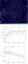 |
Fig. D.1 Upper panel: CFHTLS i′ band ~2′× 2′ image of the XLSSC 122 structure. Red circles represent the three detected objects along the line of sight. White contours are for the X-ray emission. Middle panel: spectrum of the southern star. Bottom panel: spectrum of the star close to the X-ray centre. |
We also placed in the slit another object, at ~50′′ from the X-ray centre towards the north. Nearly invisible on the i′ band image, it shows a single isolated emission line in the FORS2 spectrum at ~5436 Å. It may be an object at z ~ 2.51 with CIV in emission. It also may be Lymanα at z ~ 3.47. In this case, we may have expected to also detect CIV at ~6911 Å, but this position is heavily polluted by sky lines. We could also consider a CIII emission at z ~ 1.85 (Lymanα and CIV would be outside of our spectral range in this case, and MgII would also be heavily polluted by sky lines). Finally, it is unlikely that this line is MgII at z ~ 0.94 because we do not detect [OII].
Appendix E: Cluster pairs
To publish the full results of our super-cluster detection process, in Table E.1 we give the detected cluster pairs. We only list a sequence number as these structures are not used at all in the present paper.
List of detected cluster pairs with the FoF approach.
Appendix F: Alternative measurement of X-ray parameters
In Table F.1 we provide the parameter estimates derived from scaling relations (including the value of r500,scal which is different from the other estimate of Table 5). XLSSC 603 is not included in this table because the flux in the pn detector was equal to zero, despite the 142 counts in the MOS.
Appendix G: C3 clusters and not yet spectroscopically confirmed C1 clusters
The spectroscopically confirmed C3 objects are listed in Table G.1. In Table G.2 we also give the list of C1 candidate clusters not yet spectroscopically confirmed (too few redshifts, and BCG identification not clear). XLSSC identifications are not available most of the time because these clusters are not yet spectroscopically confirmed. Both tables are also available in the XXL Master Catalogue browser7, appended atthe end of the XXL-365-GC table.
Parameters for C3 clusters.
C1 candidate clusters not yet spectroscopically confirmed with official name, coordinates (J2000), guessed redshift, number of available spectroscopic redshifts along the line of sight, and X-ray flux and uncertainty as in XXL Paper II and in the [0.5–2] keV band.
References
- Adami, C., & Ulmer, M. P. 2000, A&A 361, 13 [NASA ADS] [Google Scholar]
- Adami, C., Russeil, D., & Durret, F. 2007, A&A 467, 459 [NASA ADS] [CrossRef] [EDP Sciences] [Google Scholar]
- Adami, C., Mazure, A., Pierre, M., et al. 2011, A&A, 526, A18 [NASA ADS] [CrossRef] [EDP Sciences] [Google Scholar]
- Adami, C., Jouvel, S., Guennou, L., et al. 2012, A&A, 540, A105 [NASA ADS] [CrossRef] [EDP Sciences] [Google Scholar]
- Adami, C., Pompei, E., Sadibekova, T., et al. 2016, A&A, 592, A7 (XXL Survey, VIII) [NASA ADS] [CrossRef] [EDP Sciences] [Google Scholar]
- Akiyama, M., Ueda, Y., Watson, M., et al. 2015, PASJ, 67, 82 [NASA ADS] [CrossRef] [Google Scholar]
- Akritas, M. G., & Bershady, M. A. 1996, ApJ, 470, 706 [NASA ADS] [CrossRef] [Google Scholar]
- Allen, S. W., Evrard, A. E., & Mantz, A. B. 2011, ARA&A, 49, 409 [NASA ADS] [CrossRef] [Google Scholar]
- Anders, E., & Grevesse, N. 1989, Geochim. Cosmochim. Acta, 53, 197 [Google Scholar]
- Baldry, I. K., Alpaslan, M., Bauer, A. E., et al. 2014, MNRAS, 441, 2440 [NASA ADS] [CrossRef] [Google Scholar]
- Balland, C., Baumont, S., Basa, S., et al. 2009, A&A, 507, 85 [NASA ADS] [CrossRef] [EDP Sciences] [Google Scholar]
- Cash, W. 1979, ApJ, 228, 939 [NASA ADS] [CrossRef] [Google Scholar]
- Chiappetti, L., Fotopoulou, C., Lidman, C., et al. 2018, A&A, 620, A13 (XXL Survey, XXVIII) [Google Scholar]
- Chow-Martínez, M., Andernach, H., Caretta, C. A., & Trejo-Alonso, J. J. 2014, MNRAS, 445, 4073 [NASA ADS] [CrossRef] [Google Scholar]
- Clerc, N., Sadibekova, T., Pierre, M., et al. 2012, MNRAS, 423, 3561 [NASA ADS] [CrossRef] [Google Scholar]
- Comastri, A., Ranalli, P., Iwasawa, K., et al. 2011, A&A, 526, L9 [NASA ADS] [CrossRef] [EDP Sciences] [Google Scholar]
- Desai, S., Armstrong, R., Mohr, J. J., et al. 2012, ApJ, 757, 83 [NASA ADS] [CrossRef] [Google Scholar]
- Eckert, D., Molendi, S., & Paltani, S. 2011, A&A, 526, A79 [NASA ADS] [CrossRef] [EDP Sciences] [Google Scholar]
- Eckert, D., Molendi, S., Owers, M., et al. 2014, A&A, 570, A119 [NASA ADS] [CrossRef] [EDP Sciences] [Google Scholar]
- Eckert, D., Ettori, S., Coupon, J., et al. 2016, A&A, 592, A12 (XXL Survey, XIII) [NASA ADS] [CrossRef] [EDP Sciences] [Google Scholar]
- Einasto, M., Einasto, J., Tago, E., Müller, V., & Andernach, H. 2001, AJ, 122, 2222 [CrossRef] [Google Scholar]
- Faccioli, L., Pacaud, F., Sauvageot, J.-L., et al. 2018, A&A, 620, A9 (XXL Survey, XXIV) [Google Scholar]
- Finoguenov, A., Watson, M. G., Tanaka, M., et al. 2010, MNRAS, 403, 2063 [NASA ADS] [CrossRef] [Google Scholar]
- Fleenor, M. C., Rose, J. A., Christiansen, W. A., et al. 2005, AJ, 130, 957 [NASA ADS] [CrossRef] [Google Scholar]
- Folkes, S., Ronen, S., Price, I., et al. 1999, MNRAS, 308, 459 [NASA ADS] [CrossRef] [Google Scholar]
- Foreman-Mackey, D., Hogg, D. W., Lang, D., & Goodman, J. 2013, PASP, 125, 306 [CrossRef] [Google Scholar]
- Fotopoulou, S., Pacaud, F., Paltani, S., et al. 2016, A&A, 592, A5 (XXL Survey, VI) [NASA ADS] [CrossRef] [EDP Sciences] [Google Scholar]
- Garilli, B., Le Fèvre, O., Guzzo, L., et al. 2008, A&A, 486, 683 [NASA ADS] [CrossRef] [EDP Sciences] [Google Scholar]
- Gelman, A., & Rubin, D. B. 1992, Statist. Sci., 7, 457 [NASA ADS] [CrossRef] [Google Scholar]
- Giles, P., Maughan, B. J., Pacaud, F., et al. 2016, A&A, 592, A3 (XXL Survey, III) [NASA ADS] [CrossRef] [EDP Sciences] [Google Scholar]
- Gioia, I. M., Maccacaro, T., Schild, R. E., et al. 1990, ApJSS, 72, 567 [CrossRef] [Google Scholar]
- Girardi, M., Aguerri, J. A. L., De Grandi, S., et al. 2014, A&A, 565, A115 [NASA ADS] [CrossRef] [EDP Sciences] [Google Scholar]
- Guennou, L., Adami, C., Durret, F., et al. 2014, A&A, 561, A112 [NASA ADS] [CrossRef] [EDP Sciences] [Google Scholar]
- Guzzo, L., Scodeggio, M., Garilli, B., et al. 2014, A&A, 566, A108 [NASA ADS] [CrossRef] [EDP Sciences] [Google Scholar]
- Hasinger, G., Cappelluti, N., Brunner, H., et al. 2007, ApJS, 172, 29 [NASA ADS] [CrossRef] [Google Scholar]
- Hinshaw, G., Larson, D., Komatsu, E., et al. 2013, ApJS, 208, 19 [NASA ADS] [CrossRef] [Google Scholar]
- Hinton, S. R., Davis, T. M., Lidman, C., et al. 2016, Astron. Comput., 15, 61 [NASA ADS] [CrossRef] [Google Scholar]
- Icke, V., & van de Weygaert, R. 1987, A&A, 184, 16 [NASA ADS] [Google Scholar]
- Jones, L. R., Ponman, T. J., Horton, A., et al. 2003, MNRAS, 343, 627 [NASA ADS] [CrossRef] [Google Scholar]
- Khosroshahi, H. G., Ponman, T. J., Jones, L. R. 2007, MNRAS, 377, 595 [NASA ADS] [CrossRef] [Google Scholar]
- Koulouridis, E., Poggianti, B., Altieri, B., et al. 2016, A&A, 592, A11 (XXL Survey, XII) [NASA ADS] [CrossRef] [EDP Sciences] [Google Scholar]
- Kundert, A., Gastaldello, F., D’Onghia, E., et al. 2015, MNRAS, 454, 161 [NASA ADS] [CrossRef] [Google Scholar]
- Le Fèvre, O., Cassata, P., Cucciati, O., et al. 2013, A&A, 559, A14 [NASA ADS] [CrossRef] [EDP Sciences] [Google Scholar]
- Lidman, C., Ardila, F., Owers, M., et al. 2016, PASA, 33, 1 (XXL Survey, XIV) [NASA ADS] [CrossRef] [Google Scholar]
- Lietzen, H., Tempel, E., Liivamagi, L. J., et al. 2016, A&A, 588, L4 [NASA ADS] [CrossRef] [EDP Sciences] [Google Scholar]
- Lieu, M., Smith, G. P., Giles, P. A., et al. 2016, A&A, 592, A4 (XXL Survey, IV) [NASA ADS] [CrossRef] [EDP Sciences] [Google Scholar]
- Liske, J., Baldry, I. K., Driver, S. P., et al. 2015, MNRAS, 452, 2087 [NASA ADS] [CrossRef] [Google Scholar]
- Mantz, A. B., Abdulla, Z., Carlstrom, J. E., et al. 2014, ApJ, 794, 157 (XXL Survey, V) [NASA ADS] [CrossRef] [Google Scholar]
- Mantz, A. B., Abdulla, Z., Allen, S. W., et al. 2018, A&A, 620, A2 (XXL survey, XVII) [NASA ADS] [CrossRef] [EDP Sciences] [Google Scholar]
- Melnyk, O., Elyiv, A., Smolcic, V., et al. 2018, A&A, 620, A6 (XXL Survey, XXI) [NASA ADS] [CrossRef] [EDP Sciences] [Google Scholar]
- Pacaud, F., Clerc, N., Giles, P. A., et al. 2016, A&A, 592, A2 (XXL Survey, II) [NASA ADS] [CrossRef] [EDP Sciences] [Google Scholar]
- Pierre, M., Valtchanov, I., Altieri, B., et al. 2004, JCAP, 09, 011 [CrossRef] [Google Scholar]
- Pierre, M., Pacaud, F., Adami, C., et al. 2016, A&A, 592, A1 (XXL Survey, I) [NASA ADS] [CrossRef] [EDP Sciences] [Google Scholar]
- Ranalli, P., Comastri, A., Vignali, C., et al. 2013, A&A, 555, A42 [NASA ADS] [CrossRef] [EDP Sciences] [Google Scholar]
- Roussel, H., Sadat, R., & Blanchard, A. 2000, A&A, 361, 429 [NASA ADS] [Google Scholar]
- Ruel, J., Bazin, G., Bayliss, M., et al. 2014, ApJ, 792, 45 [Google Scholar]
- Sandin, C., Becker, T., Roth, M. M., et al. 2010, A&A, 515, A35 [NASA ADS] [CrossRef] [EDP Sciences] [Google Scholar]
- Santos, W. A., Mendes de Oliveira, C., & Sodré, L. Jr. 2007, AJ, 134, 1551 [NASA ADS] [CrossRef] [Google Scholar]
- Scodeggio, M., Guzzo, L., Garilli, B., et al. 2018, A&A, 609, A84 [NASA ADS] [CrossRef] [EDP Sciences] [Google Scholar]
- Serna, A., & Gerbal, D. 1996, A&A, 309, 65 [NASA ADS] [Google Scholar]
- Simpson, C., Martínez-Sansigre, A., & Rawlings, S., et al. 2006, MNRAS, 372, 741 [NASA ADS] [CrossRef] [Google Scholar]
- Simpson, C., Rawlings, S., Ivison, R., et al. 2012, MNRAS, 421, 3060 [NASA ADS] [CrossRef] [Google Scholar]
- Smith, R. K., Brickhouse, N. S., Liedahl, D. A., & Raymond, J. C. 2001, ApJ, 556, L91 [NASA ADS] [CrossRef] [Google Scholar]
- Söchting, I. K., Coldwell, G. V., Clowes, R. G., Campusano, L. E., & Graham, M. J. 2012, MNRAS, 423, 2436 [NASA ADS] [CrossRef] [Google Scholar]
- Stalin, C. S., Petitjean, P., Srianand, R., et al. 2010, MNRAS, 401, 294 [NASA ADS] [CrossRef] [Google Scholar]
- Suhada, R., Song, J., Böhringer, H., et al. 2012, A&A, 537, A39 [NASA ADS] [CrossRef] [EDP Sciences] [Google Scholar]
- Ulmer, M. P., Adami, C., Covone, G., et al. 2005, ApJ, 624, 124 [NASA ADS] [CrossRef] [Google Scholar]
- Wen, Z. L., Han, J. L., & Liu, F. S. 2012, ApJS, 199, 34 [NASA ADS] [CrossRef] [Google Scholar]
- Yuan, F., Lidman, C., Davis, T. M., et al. 2015, MNRAS, 452, 3047 [NASA ADS] [CrossRef] [Google Scholar]
- Zarattini, S., Barrena, R., Girardi, M., et al. 2014, A&A, 565, A116 [NASA ADS] [CrossRef] [EDP Sciences] [Google Scholar]
r500,MT
is defined as the radius of the sphere inside which the mean density is 500 times the critical density
ρc of the Universe at the cluster’s redshift, M500,MT is then by definition equal to  .
.
Those assume an APEC v2.0.2 thermal spectrum with T = 2 keV and Z = 0.3Z⊙. The difference between the two fields comes from their average absorbing column density of nH = 2.3 × 1020 cm−2 for XXL-N and 1.25 × 1020 cm−2 for XXL-S.
All Tables
Tabulated values of the differential luminosity ([0.5–2] keV) function for the C1 sample.
Tabulated values of the cumulative luminosity ([0.5–2] keV) function for the C1 sample.
Results of the redshift measurements on the detected galaxies in the PMAS/PPak data for XLSSC 110 cluster.
Details of the PMAS/PPak observations of XLSSC 110: exposure number, run date, coordinates (J2000), air mass range.
C1 candidate clusters not yet spectroscopically confirmed with official name, coordinates (J2000), guessed redshift, number of available spectroscopic redshifts along the line of sight, and X-ray flux and uncertainty as in XXL Paper II and in the [0.5–2] keV band.
All Figures
|
Fig. 1 Redshift difference versus redshift for the ~12 000 objects measured twice within the spectroscopic survey. The two red dotted lines represent the ±3 × 600 km s−1 level (cf. Sect. 3.2). We also give the histogram of the redshift difference within the [− 0.005, 0.005] interval. |
| In the text | |
|
Fig. 2 Redshift difference versus redshift for the galaxies (at < ± 3 × σv,200 from the cluster mean redshift and within one Virial radius) measured two times within the spectroscopic survey. The two red dotted lines represent the ±3 × 600 km s−1 level. We also give the histogram of the redshift difference within the [− 0.005, 0.005] interval. |
| In the text | |
|
Fig. 3 Upper panel: y-axis, number of confirmed clusters; x-axis, number of galaxy redshifts sampling the confirmed clusters. Different colours and line styles are from different spectroscopic surveys. Bottom panel: percentage of galaxy redshifts inside the confirmed clusters coming from a given survey and for a given redshift bin. Because of multiple galaxy spectroscopic measurements, the sum of the percentages for a given redshift bin is larger than 100%. |
| In the text | |
|
Fig. 4 Comparison between the true temperature measurements (from Table 5) and estimates from the scaling relations (from Table F.1). The dotted and solid lines show the 1:1 relation and the actual regression to the data respectively. |
| In the text | |
|
Fig. 5 Distribution of the number of spectroscopic redshifts inside clusters with a redshift measurement. The insets show the redshifthistograms of these samples. Top panel: spectroscopic + photometric redshift sample (black histograms), and spectroscopic redshift sample (red histograms) clusters. Bottom panel: XXL-N (red histograms) and XXL-S (blue histograms) clusters. Photometric redshifts are used in replacement of spectroscopic redshifts in these two histograms when spectroscopic redshifts are not available. |
| In the text | |
|
Fig. 6 Distribution of the number of spectroscopic redshifts inside clusters with a redshift estimate. The insets show the redshift histograms of these samples. Top panel: C1 (red histograms), C2 (blue histograms), and C3 (green histograms) clusters. Bottom panel: clusters with also a flux estimate fainter (black histograms) and brighter (red histograms) than the reference flux completeness limit of 1.3 × 10⁻¹⁴ erg s−1 cm−2. |
| In the text | |
|
Fig. 7 X-ray luminosity ( |
| In the text | |
|
Fig. 8 Mass (in log units of M⊙) distributionof the clusters with a spectroscopic redshift estimate. Red histogram: the C1 sample; blue histogram: the C2 sample. The mass data points have been derived from scaling relations based on the cluster luminosities (cf. Sect. 4.3 and Appendix F). |
| In the text | |
|
Fig. 9 X-ray flux (F60 in log unit of erg s−1 cm−2, within a 60″ radius in the [0.5–2] keV band) distribution for the clusters having a spectroscopic redshift. Red histogram: the C1 sample; blue histogram: the C2 sample; green histogram: the C3 sample. The black vertical line is the estimated reference flux completeness limit of 1.3 × 10⁻¹⁴ erg s−1 cm−2. |
| In the text | |
|
Fig. 10 Upper panel: luminosity–temperature relation with the best-fitting models. The light blue circles show the XXL-C1-GC clusters; the best-fitting model (including selection effects) is shown by the solid black line, the 1σ uncertainty represented by the grey shaded region. The best-fitting model fitted to the data using the BCES regression is shown as the dashed line. Bottom panel: evolution of the luminosity–temperature relation for XXL-C1-GC. The XXL-C1-GC clusters are represented by the light blue circles and the best-fitting model is given by the black solid line; the grey shaded region highlights the 1σ uncertainty.The “strong” and “weak” self-similar expectations are given by the red dashed and blue dashed lines, respectively. |
| In the text | |
|
Fig. 11 Scatterplot matrix for the fit of the luminosity–temperature relation of the XXL-C1-GC sample. The posterior densities are shown along the diagonal; the 1σ, 2σ, and 3σ confidence contours for the pairs of parameters are shown in the upper right panels. The lower left panels show the Pearson’s correlation coefficient for the corresponding pair of parameters (text size is proportional to the correlation strength). |
| In the text | |
|
Fig. 12 Matrix plot comparing the 1σ, 2σ and 3σ contours for pairs of parameters of the luminosity–temperature relation, with the XXL-C1-GC and XXL-100-GC contours given by the black and red contours respectively. |
| In the text | |
|
Fig. 13 Fit contours of the luminosity–temperature relation parameters using both the XXL Paper IV mass temperature relation (based on the XXL-C1-GC sample: black contours) and the scaled relation (normalisation of the mass–temperature decreased by 20% and using the same slope as in XXL Paper IV: red contours). |
| In the text | |
|
Fig. 14 Upper panel: X-ray luminosity function ([0.5–2] keV band) of the C1 cluster sample based on the 186 C1 clusters in good pointings and with redshift information. The calculation is averaged over the whole survey volume (z in 0.0–1.3) and includes an incompleteness factor of 2.6% for the five C1 clusters without any redshift estimate. The method is the same as in XXL Paper II. For comparison, the luminosity function of the XXL brightest 100 cluster sample (XXL-100-GC) is shown with the red dashed line. Finally, the dot-dashedblue line indicates the luminosity function of the C1 sample recomputed for with the old LX − T relation of XXL Paper III, as was assumed for the XXL-100-GC sample. Lower panel: residuals of the C1 luminosity functions computed from only the northern or southern XXL field with respect to the complete luminosity function shown in the upper panel. |
| In the text | |
|
Fig. 15 Redshift evolution of the C1 X-ray luminosity function. The calculation relies on the same assumptions as for the full survey volume luminosity function of Fig. 14, but the sample is split into three redshift bins containing approximately the same number counts of clusters. The dashed lines show, for the same redshift bins, the luminosity function expected in the WMAP9 cosmology from our scaling relation model (M500,WL − T300 kpc
from XXL Paper IV and |
| In the text | |
|
Fig. 16 CFHTLS 2.4′× 2.3′ i′ image of XLSSC 110 with known galaxy members of the structure. Green circles are from the main dynamical structure, and red and white circles are from two secondary structures following the Serna–Gerbal technique. The large red circle represents a 500 kpc radius. White contours are for the X-ray emission. The given numbers are the galaxy identification in Table 10 and the redshifts of the same table (giving priority to the new redshifts we measured ourselves). |
| In the text | |
|
Fig. 17 Percentage of spectroscopic redshifts within r500,scal that are found in the two-magnitude interval fainter than the BCG, as a function of the uncertainty on the probability for a cluster to be a fossil group (given in Table 11). Inset: r′ band magnitude histogram of the galaxies without a spectroscopic redshift, and within the two-magnitude range of our FG candidates. |
| In the text | |
|
Fig. 18 Histogram of the number of magnitudes we can add to the brightest cluster member r′ magnitude in order to achieve a probability larger than 20% to have no galaxy within the defined magnitude interval (for all the spectroscopically confirmed clusters of the XXL northern area). |
| In the text | |
|
Fig. B.1 CFHTLS i′ band 4.5′× 3′ image around the XLSSC 035 confirmed z = 0.174 cluster. Green circles represent the member galaxies plus the bright foreground galaxy discussed in the text. White contours arefor the X-ray emission. |
| In the text | |
|
Fig. B.2 CFHTLS i′ band 5.5′× 3.5′ image around the XLSSC 041 confirmed z = 0.142 cluster. Magenta circles represent the member galaxies. White circles are the galaxy members of the background cluster at z = 0.557. White contours are for the X-ray emission. |
| In the text | |
|
Fig. B.3 CFHTLS i′ band 4.5′× 3′ image around XLSSC 514 and XLSSC 515 confirmed z = 0.101 and 0.169 clusters. Magenta circles represent the member galaxies of the two clusters. Figures are showing the central areas of these structures. White contours are for the X-ray emission. |
| In the text | |
|
Fig. B.4 CFHTLS i′ band 7.5′× 5′ image around XLSSC 539 confirmed z = 0.184 and 0.169 double structure. Red circles represent the member galaxies of the two components. We clearly see the central z = 0.184 structure and the other component at z = 0.169 towards the east. The large red circle represents a 500 kpc radius area. White contours are for the X-ray emission. |
| In the text | |
|
Fig. B.5 CFHTLS i′ band 4′ × 2.5′ image around XLSSC 096. Green squares represent the member galaxies of the main structure at z = 0.520 and magentacircles are the foreground structure at z = 0.203. The large red circle represents a 500 kpc radius area. White contours are for the X-ray emission. |
| In the text | |
|
Fig. B.6 CFHTLS i′ band 6.5′× 4.5′ image around XLSSC 151. Magenta circles represent the member galaxies of the main structure at z = 0.189 and blue circles those of the background structure at z = 0.280. The large red circle represents a 500 kpc radius area. White contours are for the X-ray emission. |
| In the text | |
|
Fig. B.7 CFHTLS i′ band 6.5′× 4.5′ images of two superposed structures. Magenta circles represent the member galaxies of the two structures at z = 0.263 (upper panel) and at z = 0.317 (bottom panel). The large red circle represents a 500 kpc radius area. White contours are for the X-ray emission. |
| In the text | |
|
Fig. B.8 CFHTLS i′ band 6.5′× 4.5′ image of the XLSSC 149 and 150 structures. Magenta circles represent the member galaxies of the two structures at z = 0.292. The large red circles represent 500 kpc radius areas. White contours are for the X-ray emission. |
| In the text | |
|
Fig. D.1 Upper panel: CFHTLS i′ band ~2′× 2′ image of the XLSSC 122 structure. Red circles represent the three detected objects along the line of sight. White contours are for the X-ray emission. Middle panel: spectrum of the southern star. Bottom panel: spectrum of the star close to the X-ray centre. |
| In the text | |
Current usage metrics show cumulative count of Article Views (full-text article views including HTML views, PDF and ePub downloads, according to the available data) and Abstracts Views on Vision4Press platform.
Data correspond to usage on the plateform after 2015. The current usage metrics is available 48-96 hours after online publication and is updated daily on week days.
Initial download of the metrics may take a while.