| Issue |
A&A
Volume 618, October 2018
|
|
|---|---|---|
| Article Number | A63 | |
| Number of page(s) | 32 | |
| Section | Planets and planetary systems | |
| DOI | https://doi.org/10.1051/0004-6361/201832942 | |
| Published online | 12 October 2018 | |
The GJ 504 system revisited
Combining interferometric, radial velocity, and high contrast imaging data★
1
Université Grenoble Alpes, CNRS, IPAG,
38000
Grenoble,
France
2
Aix Marseille Université, CNRS, CNES, LAM,
Marseille,
France
e-mail: mickael.bonnefoy@univ-grenoble-alpes.fr
3
School of Earth & Space Exploration, Arizona State University,
Tempe AZ
85287,
USA
4
Leiden Observatory, Leiden University,
PO Box 9513,
2300
RA Leiden,
Netherlands
5
Laboratoire Lagrange, UMR 7293 UNS-CNRS-OCA, Boulevard de l’Observatoire,
BP 4229,
06304
Nice Cedex 4,
France
6
Physikalisches Institut, Universität Bern,
Gesellschaftsstrasse 6,
3012
Bern,
Switzerland
7
Max Planck Institute for Astronomy,
Königstuhl 17,
69117
Heidelberg,
Germany
8
Maison de la Simulation, CEA, CNRS, Université Paris-Sud, UVSQ, Universiteé Paris-Saclay,
91191
Gif-sur-Yvette,
France
9
INAF–Osservatorio Astronomico di Brera,
Via E. Bianchi 46,
23807
Merate,
Italy
10
LESIA, Observatoire de Paris, PSL Research University, CNRS, Sorbonne Universités, UPMC Université Paris 06, Université Paris Diderot,
Sorbonne Paris Cité,
France
11
Astrobiology Center of NINS, 2-21-1, Osawa, Mitaka,
Tokyo,
181-8588,
Japan
12
National Astronomical Observatory of Japan, 2-21-1, Osawa, Mitaka,
Tokyo,
181-8588,
Japan
13
Department of Astronomy, Stockholm University, AlbaNova University Center,
106 91
Stockholm,
Sweden
14
Harvard University, Cambridge,
MA
02138,
USA
15
CRAL, UMR 5574, CNRS, Université de Lyon, Ecole Normale Supérieure de Lyon,
46 Allée d’Italie,
F-69364
Lyon Cedex 07,
France
16
INAF – Osservatorio Astronomico di Padova,
Vicolo dell Osservatorio 5,
35122,
Padova,
Italy
17
Geneva Observatory, University of Geneva,
Chemin des Maillettes 51,
1290
Versoix,
Switzerland
18
Department of Physics, University of Oxford, Oxford,
UK
19
Instituto de Astronomía y Ciencias Planetarias de Atacama,
Copayapu 485,
Copiap,
Atacama,
Chile
20
Institute for Astronomy, University of Hawaii,
2680 Woodlawn Drive,
Honolulu,
HI 96822,
USA
21
SUPA, Institute for Astronomy, The University of Edinburgh, Royal Observatory,
Blackford Hill,
Edinburgh,
EH9 3HJ,
UK
22
Unidad Mixta Internacional Franco-Chilena de Astronomía, CNRS/INSU UMI 3386 and Departamento de Astronomía, Universidad de Chile,
Casilla 36-D,
Santiago,
Chile
23
Office National d’Études et de Recherches Aérospatiales (ONERA), Optics Department,
BP 72,
92322
Châtillon,
France
24
Astrophysics Department, Institute for Advanced Study,
Princeton,
NJ
08544,
USA
25
Exoplanets and Stellar Astrophysics Laboratory,
Code 667, Gxsoddard Space Flight Center,
Greenbelt,
MD
20771,
USA
26
Department of Astronomy, The University of Tokyo,
7-3-1,
Hongo,
Bunkyo-ku, Tokyo,
113-0033,
Japan
27
European Southern Observatory (ESO),
Karl-Schwarzschild-Str. 2,
85748
Garching,
Germany
28
Institute for Particle Physics and Astrophysics, ETH Zurich,
Wolfgang-Pauli-Strasse 27,
8093
Zurich,
Switzerland
29
Department of Astronomy, University of Michigan, 1085 S. University Ave,
Ann Arbor,
MI
48109-1107,
USA
30
Núcleo de Astronomía, Facultad de Ingeniería y Ciencias, Universidad Diego Portales,
Av. Ejercito 441,
Santiago,
Chile
31
Escuela de Ingeniería Industrial, Facultad de Ingeniería y Ciencias, Universidad Diego Portales,
Av. Ejercito 441,
Santiago,
Chile
32
NOVA Optical Infrared Instrumentation Group,
Oude Hoogeveensedijk 4,
7991
PD Dwingeloo,
The Netherlands
Received:
2
March
2018
Accepted:
28
June
2018
Context. The G-type star GJ504A is known to host a 3–35 MJup companion whose temperature, mass, and projected separation all contribute to making it a test case for planet formation theories and atmospheric models of giant planets and light brown dwarfs.
Aims. We aim at revisiting the system age, architecture, and companion physical and chemical properties using new complementary interferometric, radial-velocity, and high-contrast imaging data.
Methods. We used the CHARA interferometer to measure GJ504A’s angular diameter and obtained an estimation of its radius in combinationwith the HIPPARCOS parallax. The radius was compared to evolutionary tracks to infer a new independent age range for the system. We collected dual imaging data with IRDIS on VLT/SPHERE to sample the near-infrared (1.02–2.25 μm) spectral energy distribution (SED) of the companion. The SED was compared to five independent grids of atmospheric models (petitCODE,Exo-REM, BT-SETTL, Morley et al., and ATMO) to infer the atmospheric parameters of GJ 504b and evaluate model-to-model systematic errors. In addition, we used a specific model grid exploring the effect of different C/O ratios. Contrast limits from 2011 to 2017 were combined with radial velocity data of the host star through the MESS2 tool to define upper limits on the mass of additional companions in the system from 0.01 to 100 au. We used an MCMC fitting tool to constrain the companion’sorbital parameters based on the measured astrometry, and dedicated formation models to investigate its origin.
Results. We report a radius of 1.35 ± 0.04 R⊙ for GJ504A. The radius yields isochronal ages of 21 ± 2 Myr or 4.0 ± 1.8 Gyr for the system and line-of-sight stellar rotation axis inclination of 162.4−4.3+3.8 degrees or 186.6−3.8+4.3 degrees. We re-detect the companion in the Y2, Y3, J3, H2, and K1 dual-band images. The complete 1–4 μm SED shape of GJ504b is best reproduced by T8-T9.5 objects with intermediate ages (≤ 1.5Gyr), and/or unusual dusty atmospheres and/or super-solar metallicities. All atmospheric models yield Teff = 550 ± 50 K for GJ504b and point toward a low surface gravity (3.5–4.0 dex). The accuracy on the metallicity value is limited by model-to-model systematics; it is not degenerate with the C/O ratio. We derive log L∕L⊙ = −6.15 ± 0.15 dex for the companion from the empirical analysis and spectral synthesis. The luminosity and Teff yield masses of M = 1.3−0.3+0.6 MJup and M = 23−9+10 MJup for the young and old age ranges, respectively. The semi-major axis (sma) is above 27.8 au and the eccentricity is lower than 0.55. The posterior on GJ 504b’s orbital inclination suggests a misalignment with the rotation axis of GJ 504A. We exclude additional objects (90% prob.) more massive than 2.5 and 30 MJup with semi-major axes in the range 0.01–80 au for the young and old isochronal ages, respectively.
Conclusions. The mass and semi-major axis of GJ 504b are marginally compatible with a formation by disk-instability if the system is 4 Gyr old. The companion is in the envelope of the population of planets synthesized with our core-accretion model. Additional deep imaging and spectroscopic data with SPHERE and JWST should help to confirm the possible spin-orbit misalignment and refine the estimates on the companion temperature, luminosity, and atmospheric composition.
Key words: techniques: high angular resolution / stars: fundamental parameters / techniques: radial velocities / techniques: interferometric / planets and satellites: atmospheres / planets and satellites: formation
© ESO 2018
1 Introduction
The most recent formation and dynamical evolution models of the solar system (e.g., Walsh et al. 2011; Raymond & Izidoro 2017) propose that the wide-orbit giant planets (Jupiter, Saturn) have largely influenced the composition and/or the architecture of the inner solar system. Those models are guided by the population of exoplanets established below ~8 au mainly through transit and radial velocity surveys (e.g., Udry & Santos 2007; Marcy et al. 2008; Wright et al. 2009; Coughlin et al. 2016; Crossfield et al. 2016; Morton et al. 2016). Several pieces of evidence support the universality of the core-accretion (CA; Pollack et al. 1996; Alibert et al. 2004) formation scenario in this separation range (e.g., Mordasini et al. 2009; Bowler et al. 2010). Some systems (planets with large sky-projected obliquities; packed systems; see Winn et al. 2005; Carter et al. 2012; Bourrier et al. 2018) highlight the dramatic role played by dynamical interactions such as disk-induced migration (for a review, see Baruteau et al. 2014), and planet–planet scattering (Nagasawa et al. 2008; Ford & Rasio 2008) in stabilizing or (re)shaping the system architectures in the first astronomical units.
Our knowledge of the formation and dynamical evolution of planetary systems at large separation (>8 au) is limited. Itrelies for the most part on the direct imaging (DI) method whose sensitivity to low-mass companions increases on nearby (d < 150 pc) young systems (age < 150 Myr). At these ages, planets can still be hot and self luminous from their formation (depending on the accretion phase, e.g., the so called “hot” and “cold” start conditions; Marley et al. 2007; Mordasini et al. 2017) and be detected at favorable contrasts in the near-infrared (NIR; 1–5 μm). The implementation of differential methods (Racine et al. 1999; Marois et al. 2000, 2006) on 8 m ground-based telescopes equipped with adaptive optics in the late 2000s led to the breakthrough detections of massive (5–13 MJup) Jovian planets at short physical separations (9–68 au) around the young (~ 17−30 Myr) intermediate-mass (AF) stars HR 8799 (Marois et al. 2008, 2010), β Pictoris (Lagrange et al. 2009, 2010), and HD 95086 (Rameau et al. 2013a,b). Systems such as HR8799 challenge the CA paradigm whose timescales are too long at large orbital radii compared to the circumstellar disk lifetimes (Haisch et al. 2001). The gravitational instability scenario (hereafter GI; e.g., Boss 1997; Forgan & Rice 2013) has been proposed as an alternative to solve that issue. But the GI model outcomes depend on their sophistication (e.g., Kratter et al. 2010; Müller et al. 2018) and some fine tuning is possible (e.g., Baehr et al. 2017; Boss 2017).
The model development can be guided by the discovery of new systems and by the statistics inferred from the DI surveys (e.g., Janson et al. 2012; Vigan et al. 2017). The second generation of DI instruments SPHERE (Beuzit et al. 2008), GPI (Macintosh et al. 2008), and SCExAO (Jovanovic et al. 2015) have been designed to detect fainter companions closer to their stars (10−6 contrasts at 500 mas). Ambitious surveys such as the SpHere INfrared survey for Exoplanets (SHINE) aim at building a meaningful statistics (400−600 stars) on the occurrence and properties of the giant planets from 5 au. These instruments have already detected two more planetary systems around the AF-type stars 51 Eri and HIP 65426 (Macintosh et al. 2015; Chauvin et al. 2017) and four BD companions around F and G-type stars (Konopacky et al. 2016; Milli et al. 2017; Cheetham et al. 2018a,b).
The high-precision astrometry of these instruments brings constraints on the companion orbital parameters and system achitectures in spite of the slow orbital motions (Zurlo et al. 2016; Vigan et al. 2016; Maire et al. 2016a; Rameau et al. 2016; Wang et al. 2016; Delorme et al. 2017c; Chauvin et al. 2018). Stringent detection limits can be derived from these observations at multiple epochs and be combined with radial velocity data of the host star to provide insightful constraints on the masses of undetected companions (Lannier et al. 2017; Chauvin et al. 2018) over all possible semi-major axes.
SPHERE and GPI have extracted high-quality low-resolution (R ~ 30− 300) NIR (1–2.5 μm) spectra of most of the known substellar companions found at projected separations below 100 au (e.g., Bonnefoy et al. 2014c; Hinkley et al. 2015a; De Rosa et al. 2016; Zurlo et al. 2016; Samland et al. 2017; Delorme et al. 2017c; Chilcote et al. 2017; Mesa et al. 2018). In addition, SPHERE uniquely allows for dual-band imaging of the coolest companions in narrow-band filters sampling the H2O and CH4 absorptions appearing in their SEDs (Vigan et al. 2010, 2016).
An empirical understanding of the companions’ nature can be achieved through the comparison of their spectra and photometry to those of the many ultracool dwarfs found in the field (e.g., Mace et al. 2013a; Best et al. 2015; Robert et al. 2016) or in young clusters (e.g., Best et al. 2017; Lodieu et al. 2018). Most young planet and BD companions studied so far have spectral features characteristic of M- and L-type objects with hot atmospheres 1000 ≤ Teff ≤ 3000 K. Some peculiar features appear such as the red spectral slopes and shallow molecular absorption bands that might be caused by the low surface gravity of the objects (e.g. Bonnefoy et al. 2016; Delorme et al. 2017c).
Only three companions (51 Eri b, GJ 758b, HD 4113C) with Teff ≤ 800K and noticeable methane absorptions typical of T-type dwarfs have been detected and/or characterized with the planet imaging instruments so far (Vigan et al. 2016; Samland et al. 2017; Rajan et al. 2017; Cheetham et al. 2018a). The companions 51 Eri b and GJ 758b exhibit peculiar colors (Vigan et al. 2016; Nilsson et al. 2017; Samland et al. 2017; Rajan et al. 2017) that do not match any known object. Both the low surface gravity (e.g., 51 Eri b) and non-solar atmospheric abundances might explain these spectrophotometric properties. Chemical enrichments are indeed predicted to happen at formation (e.g., Öberg & Bergin 2016; Mordasini et al. 2016; Samland et al. 2017). The empirical understanding of these objects is limited by the small number of young T-type objects identified to date (Luhman et al. 2007; Naud et al. 2014; Gagné et al. 2015, 2017, 2018a) or found in metal-rich environments (Bouvier et al. 2008).
Atmospheric models aim at providing a global understanding of the physical, chemical, and dynamical processes atplay in planetary and BD atmospheres. Models face difficulties matching the NIR colors (J− K, J−H) of objects at the so-called T/Y transition corresponding to a Teff of around 500 K (e.g., Bochanski et al. 2011), but promising new ingredients have been introduced to solve this issue. One is the formation of a cloud deck made of alkali salts and sulfides (Morley et al. 2012) whose impact peaks at Teff = 500−600 K. Another group chose, rather, to introduce a modification of the temperature gradient caused by fingering convection (Tremblin et al. 2015; Leggett et al. 2016). The effect of the fingering instability on the thermal gradient, however, has recently been questioned (Leconte 2018). The few detected companions at the T/Y transition are precious benchmarks for atmospheric models because of the known ages and distances of the host stars.
A faint companion was resolved in 2011 at 2.5′′ projected separation (43.5 au) from the nearby (17.56 ± 0.08 pc; van Leeuwen 2007) G0-type star GJ 504 (Kuzuhara et al. 2013) in the course of the “Strategic Exploration of Exoplanets and Disks with Subaru” (SEEDS) survey (Tamura 2009). The companion mass was estimated to be  , making it the first Jovian exoplanet resolved around a solar-type star. This mass estimate is nonetheless tied to the host star age of
  Myr inferred from gyrochronology and activity indicators. Some tension existed between this age and the one derived from evolutionary tracks (Kuzuhara et al. 2013), but the authors argued that a reliable isochronal age could not be inferred because it would have relied on Teff measurements of the star for which inconsistent values exist in the literature (e.g., Valenti & Fischer 2005; da Silva et al. 2012). Fuhrmann & Chini (2015) derived their own Teff estimate from the modeling of a high-resolution optical spectrum of the star. They found an isochronal age of
  Gyr, implying a mass of ~24 MJup for the companion. D’Orazi et al. (2017b) made a strictly differential (line-by-line) analysis of GJ 504A spectra to derive new atmospheric parameters and abundances. They confirmed that the star has a metallicity above solar ([Fe∕H] = 0.22 ± 0.04) and inferred an isochronal age of
  Gyr, leaving GJ 504b in the brown-dwarf mass regime.
The companion has NIR broad-band photometry (J, H, Ks, L′) similar to late T-type objects (Kuzuhara et al. 2013). Janson et al. (2013) obtained differential imaging data that showed a strong methane absorption at 1.6 μm which confirms the cool atmosphere of GJ 504b. Complementary observations (Skemer et al. 2016) were obtained with LBT/LMIRCam at wavelengths of 3.71, 3.88, and 4.00 μm. Skemer et al. (2016) estimate a Teff = 543 ± 11 K consistent with an object close to the T/Y transition. The analysis also reveals that the companion might be enriched in metals with respect to GJ 504A. They also find a low surface gravity which is more consistent with the age estimated by Kuzuhara et al. (2013). However, they did not study the effect of possible systematics related to the choice of the atmospheric models used to interpret the companion photometry. GJ 504A is bright (V = 5.19; Kharchenko et al. 2009) and observable from most northern and southern observatories (Dec = +09.42°). Consequently, the system is suitable to observations with an array of techniques. This paper aims at revisiting the system properties based on interferometric measurements, high-contrast imaging observations, and existing and new radial-velocity (RV) data. We present the observations and the related data processing in Sect. 2. We derive a new age estimate for the system in Sect. 3. We analyze the companion photometric properties following an empirical approach (Sect. 4) and using atmospheric models (Sect. 5). Section 6 summarizes the mass estimates of GJ504b that can be inferred from the analysis presented in the previous sections. In Sect. 7, we exploit the companion astrometry, the RV measurements, and the interferometric radius of GJ 504A to study the system architecture. We discuss our results in Sect. 8 and summarize them in Sect. 9.
2 Observations
2.1 SPHERE high-contrast observations
We observed GJ 504 on seven different nights with the SPHERE instrument mounted on the VLT/UT3 (Table 1) as part of the guaranteed time observation (GTO) planet search survey SHINE (Chauvin et al. 2017). All the observations were acquired in pupil-tracking mode with the 185 mass-diameter apodized-Lyot coronograph (Carbillet et al. 2011; Guerri et al. 2011).
The target was observed on May 6, 2015, June 3, 2015, March 29, 2016, and February 10, 2017 with the IRDIFS mode of SPHERE. The mode enables operation of the IRDIS instrument (Dohlen et al. 2008) in dual-band imaging mode (DBI; Vigan et al. 2010) with the H2H3 filters, and the integral field spectrograph (IFS; Claudi et al. 2008) in Y−J (0.95−1.35 μm, Rλ ~ 40) mode in parallel. The companion lies inside the circular field of view (FOV) of ~5′′ radius. It is however outside of the 1.7′′ × 1.7′′ IFS FOV.
We obtained additional observations with the IRDIFS_EXT mode on June 5, 2015. The mode enables DBI with the K1K2 filters (Table 1) and the simultaneous use of the IFS in the Y−H mode (0.95−1.64 μm, Rλ = 30). GJ 504 was then re-observed on June 6 and 7, 2015 with IRDIS and the DBI Y2Y3 and J2J3 filters (Table 1).
We collected additional calibration frames with the waffle pattern created by the deformable mirror for the May and June 2015 epochs. Those frames were used to ensure an accurate registration of the star position behind the coronagraph. The waffle pattern was maintained during the whole sequence of 2016 and 2017 IRDIFS observations to allow a registration of the individual frames along the deep-imaging sequence. We also collected nonsaturated exposures of the star before and after the sequence of coronographic exposures for astrometric and photometric extraction of point sources.
The IRDIS and IFS datasets were reduced at the SPHERE Data Center (DC; Delorme et al. 2017b) using the SPHERE Data Reduction and Handling (DRH) pipeline (Pavlov et al. 2008). The DRH carried out the basic corrections for bad pixels, dark current, and flat field. The DC performed an improved wavelength calibration, a correction of the cross-talk, and removal of bad pixels for the IFS data (Mesa et al. 2015). It also applied the anamorphism correction to the IRDIS data. We registered the frames fitting a two-dimentional moffat function to the waffles. We temporally binned some of the registered cubes of IRDIS frames to ensure we could run the angular differential imaging (ADI; Marois et al. 2006) algorithms efficiently (binning factors of 2, 4, and 8 for the K1K2, J2J3, and Y2Y3 data; factors of 7 and 2 for the May 2015 and June 2015 H2H3 data). We selected the resulting IFS datacubes based on the ratio of average fluxes in an inner and an outer ring centered on 75 and 597 mas separation to ensure that we kept the frames with the best Strehl ratio (flux ratio ≥ 1.3). Conversely, we selected 80% (H2H3, K1K2, J2J3 datasets) to 60% (Y2Y3 dataset) of the frames with the lowest halo values beyond the AO correction radius where GJ 504b lies (e.g., in a ring located between 19 and 26 full-width-at-half-maxima).
The absolute on-sky orientation of the instrument and the detector pixel scale were calibrated as part of a long-term monitoring conducted during the GTO (Maire et al. 2016a,b). The values are reported in Table 2.
We used the Specal pipeline (Galicher et al 2018) to apply the ADI steps on the IRDIS data. We applied the Template Locally Optimized Combination of Images (TLOCI; Marois et al. 2014) algorithm to extract the photometry and astrometry of the companion and to derive detection limits. The algorithm has been shown to extract the flux and position of such companions with a high fidelity (Chauvin et al., in prep.). We also used the principal component analysis (PCA; Soummer et al. 2012) implemented in Specal and ANDROMEDA (Mugnier et al. 2009; Cantalloube et al. 2015) algorithms to confirm our results. We processed the IFS data with a custom pipeline exploiting the temporal and spectral diversity (Vigan et al. 2015). The pipeline derived detection limits following the estimation of the flux losses based on the injection of fake planets with flat spectra. The sensitivity curves account for the small-number statistics affecting the noise estimates at the innermost working angles (Mawet et al. 2014).
The Y 3, J3, H2, and K1 filters sample the main emission peaks of cold companions (“on-channels”) while the central wavelengths of the Y 2, J2, H3, and K2 filters are chosen to sample the molecular absorptions. The companion is therefore re-detected in the “on” channels with signal-to-noise ratios (S/Ns) ranging from 10 to 46 (Fig. 1). We also re-detect the object in the Y 2 (Δ Y2 = 16.71 ± 0.16 mag) channel at a S/N of 7. To conclude, we also tentatively re-detect the object in the H3 band in the May 2016 data, which are the deepest obtained on the system with SPHERE. We considered the photometry extracted from the H3 channel as an upper limit in Sects. 4 and 5 to be conservative. We also derive upper limits in the J2 and K2 channels using the injection of artificial planets.
The PCA and ANDROMEDA photometry confirms the contrasts and astrometry found with the TLOCI algorithm. Table 2 summarizes the astrometry extracted from the data using TLOCI. The June 2015 astrometry obtained with the different filter pairs on consecutive days are consistent. We model these measurements in Sect. 7.1. The final contrasts were converted to apparent magnitudes (Table 3) using the star photometry estimated for the SPHERE/IRDIS pass-bands (Appendix A).
We converted the SPHERE apparent magnitudes of GJ 504b to flux densities using a spectrum of Vega (Hayes 1985; Mountain et al. 1985), the filter passbands1, and atmospheric extinction curves computed with the SKYCALC tool for our observing conditions (Noll et al. 2012; Jones et al. 2013). We followed this procedure to convert the J, H, K, L′, CH4S, and L photometry from Kuzuhara et al. (2013) and Janson et al. (2013)2. Finally, we directly used the zero points and magnitudes reported in Skemer et al. (2016) to compute the L_NB6, L_NB7, and L_NB8 fluxdensities. Table 3 summarizes the companion apparent magnitudes and flux densities used in this study.
Log of SPHERE observations.
GJ 504b astrometry.
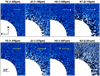 |
Fig. 1 High-contrast images of the immediate environment of GJ 504A obtained with the DBI filters ofIRDIS and using the TLOCI angular differential imaging algorithm. The star center is located in the lower-left corner of the images. GJ 504b is re-detected (arrow) into the Y 2, Y 3, J3, H2, and K1 bands. The companion is tentatively re-detected in the H3 channel. The H2-H3 images correspond to the March 2016 data. |
Apparent magnitudes and flux densities of GJ 504b.
2.2 Radial velocity
We obtained 38 spectra between March 31, 2013, and May 23, 2016, with the SOPHIE spectrograph (Bouchy & Sophie Team 2006) mounted on the OHP 1.93 m telescope. The spectra cover the 3872–6943 Å range with a R ~ 75 000 resolution. The data were reduced using the Software for the Analysis of the Fourier Interspectrum Radial velocities (SAFIR; Galland et al. 2005). From the fit of the cross-correlation function, we derive a v sin i of 6.5 ± 1 km s−1, in agreement with the value (6 ± 1 km s−1) reported in D’Orazi et al. (2017b). The data reveal radial-velocity variations with amplitudes greater than 100 m s−1 that we model in Sect. 8.1.2. The SOPHIE data are not enough to precisely measure the period of the variations but they are compatible with the star rotation period measured by Donahue et al. (1996). To complementthe SOPHIE data, we also used 57 archival RV data points from the long-term monitoring of the star obtained as part of the Lick planet search survey. They span from June 12, 1987 to February 2, 2009 (Fischer et al. 2014).
2.3 Interferometry
We observed GJ504 on June 23–25, 2017 with the VEGA instrument (Mourard et al. 2009; Ligi et al. 2013) at the CHARA interferometric array (ten Brummelaar et al. 2005). We used the VEGA medium spectral resolution mode (~6000) and selectedthree spectral bands of 20 nm centered at 550, 710, and 730 nm. We recorded seven datasets with the E2W1W2 telescope triplet, allowing us to reach baselines spanning from about 100 to 220 m. Each target observation of about 10 min is interspersed with observations of reference stars to calibrate the instrumental transfer function. We used the JMMC SearchCal3 service (Bonneau et al. 2006) to select calibrators that are bright and small enough, and close to the target: HD 110423 (whose uniform-disk angular diameter in R band equals 0.250 ± 0.007 mas according to Bourges et al. 2017) and HD 126248 (0.362 ± 0.011 mas).
We used the standard VEGA data-reduction pipeline (Mourard et al. 2009) to compute the calibrated squared visibility of each measurement. Those visibilities were fitted with the LITpro4 tool to determine a uniform-disk angular diameter θUD = 0.685 ± 0.019 millisecond of arc (mas). We used the Claret tables (Claret & Bloemen 2011) to determine the limb-darkened angular diameter θLD = 0.71 ± 0.02 mas using a linear limb-darkening law in the R band for an effective temperature ranging from 6000 to 7000 K (limb-darkening coefficient of 0.44). Assuming a parallax of 56.95 ± 0.26 mas (van Leeuwen 2007), we deduced a radius of R⋆ = 1.35 ± 0.04 R⊙ for GJ 504A.
3 Revised stellar properties
We compared the radius and the star luminosity derived in Appendix A to the PARSEC isochrones (Bressan et al. 2012) for a Z = 0.024 (Fig. 2) corresponding to the [Fe/H] = 0.22 ± 0.04 dex of GJ 504A(D’Orazi et al. 2017b). The tracks were generated using the CMD3.0 tool5. The 1 − σ uncertainty on L and R are consistent with two age ranges for the system: 21 ± 2 Myr and 4.0 ± 1.8 Gyr, according to these models. We also infer a new mass estimate of 1.10–1.25 M⊙ for the star. Wefind similar solutions using the DARTMOUTH models (Dotter et al. 2008). These isochronal ages are inconsistent with the intermediate age reported in Kuzuhara et al. (2013). The old age range overlaps with the one reported in Fuhrmann & Chini (2015) and D’Orazi et al. (2017b). The young age estimate had been neglected in Fuhrmann & Chini (2015) and was not discussed further in D’Orazi et al. (2017b). We re-investigate below how our isochronal age estimates fit with the other age indicators in light of the measured metallicity of the host-star (D’Orazi et al. 2017b) and recent work on clusters. The Barium abundance is known to decrease with stellar age (e.g., D’Orazi et al. 2009; Biazzo et al. 2017). The value for GJ 504A ([Ba∕Fe] = -0.04 ± 0.01 ± 0.03dex; D’Orazi et al. 2017b) is compatible with those of thin-disk stars (Delgado Mena et al. 2017). It is clearly at odds with the one derived for 10–50 Myr-old stars in associations and clusters (D’Orazi et al. 2009, 2017a; De Silva et al. 2013; Reddy & Lambert 2015). The kinematics of GJ 504 is also known to be inconsistent with young moving groups (YMG) or any known young open clusters (Kuzuhara et al. 2013; D’Orazi et al. 2017b) which are the only groups of young stars with distances compatible with that of GJ 504A. Stars from young nearby associations and from young clusters (<150 Myr) are generally restricted to solar metallicity values while GJ 504A has a super solar metallicity (e.g., D’Orazi & Randich 2009; Biazzo et al. 2012, 2017; Spina et al. 2017). The Hyades super-cluster is the closest group of metal-rich stars to GJ 504A. But the kinematics of GJ 504A is incompatible with these stars, in particular the V heliocentric space velocity (Montes et al. 2001)and the ages of these clusters are in any case at odds with those inferred from the tracks. The BANYAN Σ tool (Gagné et al. 2018b) yields a null probability of membership to the 27 nearby (≤ 150 pc) associations (NYA; including the Hyades), considered, and predicts the system to belong to the field (99.9% probability).
D’Orazi et al. (2017b) report stellar ages of 440 and 431 Myr from the log  and log LX /Lbol of GJ 504A using the Mamajek & Hillenbrand (2008) calibrations. The
  index of GJ 504A (− 4.45 dex; Radick et al. 1998) is in fact still compatible with those of some late-F/early-G stars (HIP 490, HIP 1481) from the Tucana–Horologium association (45 ± 4 Myr; Mamajek & Hillenbrand 2008; Bell et al. 2015) and may also reside within the envelope of values of Sco-Cen stars (11–17 Myr; Chen et al. 2011; Pecaut et al. 2012). The
  is also compatible with an age younger than 1.45 Gyr set by the stellar activity in the open cluster NGC 752. That upper limit is not consistent with the old isochronal age of GJ 504A (Fig. 2 of Pace 2013), but it does not account for the possible impact of GJ504 enhanced metallicity (Rocha-Pinto & Maciel 1998) and for the possible long-term activity cycles (>30 years) of the star whose existence has not been investigated thus far. Kuzuhara et al. (2013) argued that the X-ray activity of GJ 504A (Lx ∕Lbol = −4.42 dex; Hünsch et al. 1999) is less reliable than the
  index because of the temporal baseline which is much shorter than the one of the Calcium line measurement (while the two age indicators are correlated; Sterzik & Schmitt 1997). We do not discuss this indicator any further.
The Lithium line of GJ 504A has previously been used by Kuzuhara et al. (2013) to infer an age range of 30–500 Myr. In fact, different values for the abundance and equivalent widths have been reported for the star (equivalent width ranging from 81 to 83.1 mÅ; A(Li) = 2.74–2.91; Balachandran 1990; Favata et al. 1996; Takeda & Kawanomoto 2005; Ghezzi et al. 2010b; Ramírez et al. 2012). The spread is likely related to the uncertainty in the line-fitting method, atmospheric parameter uncertainties, and atmospheric models used (Honda et al. 2015). Lithium is also known to be a crude age estimator at the intrinsic mass and Teff of the star (Kuzuhara et al. 2013). The Li abundance of GJ 504A is in fact still compatible with the values reported for the Sco-Cen stars (Chen et al. 2011), but, conversely, it is consistent with some 1.1–1.3 M⊙ stars of thewell-characterized solar-metallicity cluster NGC 752 (Fe/H = + 0.01 ± 0.04; Sestito et al. 2004; Castro et al. 2016) and of the metal-enriched ~3 Gyr old cluster NGC 6253 (Fe/H = + 0.43 ± 0.01; Anthony-Twarog et al. 2010; Cummings et al. 2012).
Kuzuhara et al. (2013) derive an age of  Myr for the system using the rotation period and various gyrochronology relations (Barnes 2007; Mamajek & Hillenbrand 2008; Meibom et al. 2009). It is possible to derive the age of stars with a convective envelope from a measured rotation period only if they belong to the “I sequence” of slow rotators. These relations are well established and robust for such solar-type stars. With a rotation period of 3.33 days for a spectral type of G0, GJ504 is a fast rotator, and therefore belongs to the “C sequence” of fast rotators as defined in Barnes (2003), or has just reached the “I sequence”. The significant probability that GJ504 is a fast rotator means the calibrated gyrochronological relations used to directly measure its age with associated error bars are not reliable. This is confirmed by observations and model realizations (e.g., Gallet & Bouvier 2013; Gallet & Bouvier 2015) that show that G stars with a period of 3.3 days can have any age between 1 and 200 Myr. Conversely, gyrochronology provides a very robust upper limit on the age of such objects at the border between the I and C sequences, which by design have to be younger than the age at which fast rotators of a given mass have all converged toward the “I sequence” of slow rotators. Barnes (2003) and Meibom et al. (2009) show that G-type star convergence time is typically ~150 Myr. Close inspection of the M34 rotation sequence derived by Meibom et al. (2011) shows that all G stars of this cluster have turned into slow rotators. This means that if the rotation period of GJ504A derived by Donahue et al. (1996) is correct, then the star is probably younger than 150 Myr and the age of M34 (~220 Myr) is a conservative upper limit.
Table 4 summarizes the ages derived from the different indicators. None of the two possible isochronal age ranges can be firmly excluded. Asteroseismology might disentangle between our solutions (e.g., Silva Aguirre et al. 2015). We will consider both age ranges in the following sections. In Sect. 8.1, we discuss two scenarios to explain the divergent conclusions from the age indicators.
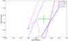 |
Fig. 2 Position of GJ504 in the Hertzsprung–Russell diagram. The constraints on the fundamental parameters are indicated by the 1σ-error box (log(L∕L⊙), R⋆). PARSEC isochrones for [Fe/H] = 0.22 ± 0.08 dex (Z = 0.024, Y = 0.29) are overplotted in blue lines for the old age solution, and in purple for the young age solution. |
Summary of the different diagnostics on the age of GJ 504A.
4 Empirical analysis of GJ 504b photometry
The SPHERE photometry more than doubles the number of photometric data points sampling the NIR (1–2.5 μm) SED (Kuzuhara et al. 2013; Janson et al. 2013) of GJ 504b. The H2−H3 color confirms the detection of a 1.6 μm methane absorption in GJ 504b’s atmosphere (Janson et al. 2013). The Y 2−Y 3 color of GJ 504b is modulated by the red wing of the potassium doublet at 0.77 μm (Allard et al. 2007). The J2−J3 and K1−K2 colors indicate that the companion has strong additional methane and water bands at 1.1 and 2.3 μm. The IRDIS photometry allows for a detailed comparison of GJ 504b to the large set of brown dwarf and young giant planets for which NIR spectra are available.
Figure 3 shows GJ 504b photometry in two selected color-magnitude diagrams (CMDs) exploiting the IRDIS photometry.Appendix C details how the CMDs are created. Late T-type companions with some knowledge on their metallicity are shown for comparison (light blue squares, see Appendix B). GJ 504b has a similar Y, J, H, and K-band luminosity and Y 3−Y 2, Y 3−J3, J3−H2, and Y 3−H2 colors as those of T8.5–T9 objects. Thecompanion ξ UMa C has the closest absolute J3 and H2 magnitude to GJ 504b, but the latter has redder H2−H3 colors indicative of a suppressed 1.6 μm CH4 absorption that might be related to sub-solar metallicity. GJ 504b J and H-band luminosity are consistent with those of the T9 standard UGPSJ072227.51-054031.2 (Lucas et al. 2010; Cushing et al. 2011). The upper limits on the J2−J3, H2−H3, and K1−K2 colors are close to those of late-T dwarfs.
We overlay GJ 504b IRDIS photometry in color–color diagrams (CCD; see Appendix C for details) corresponding to the SPHERE filter sets (Fig. 4). The late T-type benchmark objects (Appendix B) are packed in the J3-H2/Y3-J3 CCD despite the different metallicity of these objects. GJ 504b has a placement compatible with those objects; it has redder colors than most early Y dwarfs. Conversely, the benchmark companions with sub-solar metallicities have bluer colors in the J3-K1/H2-K1 CCD diagram than those with solar-metallicities for a given spectral type. The K1-band colors are indeed expected to be modulated by the pressure-induced absorptions of H2 which is in turn related to the metallicity and gravity. GJ 504b has redder colors than the T9 standard UGPSJ072227.51-054031.2 despite the fact that the two objects share the same luminosity (see below). It has a similar placement to the T8 companion Ross 458C whose host star is sharing the same metallicity range as GJ 504A but has an age (150–800 Myr; Burgasser et al. 2010) intermediate between the two age ranges derived in Sect. 3. Three other late-T objects have similar deviant colors: WISEP J231336.41-803701.4 (Burgasser et al. 2011), CFBDSIR J214947.2-040308.9 (Delorme et al. 2012), and 51 Eri b (Macintosh et al. 2015). CFBDSIR2149-04 is possibly younger than the field and/or metal enriched (Delorme et al. 2017a). The planet 51 Eri b is orbiting a young star (Montet et al. 2015) and is proposed to be metal-enriched (Samland et al. 2017). Those objects confirm that the gravity and/or the metallicity induces a shift toward redder colors in that CCD.
We used the G goodness-of-fit indicator (Cushing et al. 2008) to compare the photometry of GJ 504b to those of reference objects (Fig. 5).
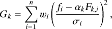 (1)
(1)
where f and σ are the observed photometry of GJ 504b and associated error, and w are the filter widths. Fk corresponds to the photometry of the template spectrum k. αk is a multiplicative factor between the companion photometry and the one of the template which minimizes Gk.
The exclusion of the K-band photometry from the fit allows the comparison to be extended to the Y dwarf domain where the K band flux of those objects is fully suppressed. The reference photometry is taken from the SpeXPrism library (Burgasser 2014) in addition to Cushing et al. (2014), Mace et al. (2013a), and Schneider et al. (2015). We also added the photometry of peculiar late-T dwarfs described in Appendix B. Figure 6 provides a visual comparison of the fit for some objects of interest. We confirm that the overall NIR luminosity of the companion is best represented by the T9 standard UGPSJ072227.51-054031.2 (Lucas et al. 2010). Companions with super-solar metallicity and/or cloudy atmospheres tend to have reduced G values compared to analogs with depleted metals. The T8 dwarf WISEA J032504.52–504403.0 produces the best fit of the YJH band flux; it is estimated to have a 100% cloudy atmosphere with low surface gravity (log g = 4.0) and be on the younger end of the age range (0.08–0.3 Gyr) of all considered objects in Schneider et al. (2015). The intermediate age and metal-rich companion ROSS 458C produces an excellent fit of the Y - to K-band fluxes of GJ 504b, but it is clearly more luminous.
We conclude that GJ 504b is a T object with peculiar NIR colors that could be attributed to low surface gravity and/or enhanced metallicity. We use atmospheric models in the following section to further explore this latter findings.
Using the  mag and
  mag of T
 dwarfs from Dupuy & Kraus (2013), we find a log
 and a log
 for GJ 504b, respectively6. The bolometric corrections might however not be appropriate for the peculiar SED of GJ 504b because it corresponds to the averaged values for “regular” dwarfs in spectral type bins. Therefore, we considered the log (L∕L⊙) = −6.20 ± 0.03 of the T9 object UGPS J072227.51-054031.2 (Dupuy & Kraus 2013) and the flux-scaling factor α =1.04 value found above to estimate a log (L∕L⊙) = −6.18 ± 0.03 dex for GJ 504b. If the T8.5 companion Wolf 940B is used instead (log (L∕L⊙) = −6.01 ± 0.05; Leggett et al. 2010), we find a log (L∕L⊙) = −6.23 ± 0.05 dex for GJ 504b.
 |
Fig. 3 Color-magnitude diagrams for the SPHERE/IRDIS photometry. The benchmark T-type companions are overlaid (full blue symbols). Their properties are summarized in Appendix B. |
 |
Fig. 4 Color–color diagram using the SPHERE/IRDIS photometry. The green stars correspond to dusty and/or young dwarfs at the L/T transition. The yellow stars correspond to the benchmark T-type companions and isolated objects listed in Table A.2. |
 |
Fig. 5 Goodness-of-fits (G) corresponding to the comparison of GJ504b photometry to those of empirical objects in the Y 2 to H2 bands (top) and from the Y 3 to K2 bands (bottom). The blue stars correspond to benchmark T-type companions while the pink ones correspond to peculiar free-floating T-type objects (see Appendix B). |
 |
Fig. 6 Visual comparison of the SED of GJ 504b (green squares) to that of T-type companions observed with VLT/SPHERE, of benchmark companions with various metallicities, and of cloudy T dwarfs. The laying bars correspond to the flux of the template spectra averaged over the filter passbands whose transmission is reported at bottom. |
5 Atmospheric properties of GJ 504b
5.1 Forward modeling with the G statistics
5.1.1 Model description
We considered five independent grids of synthetic spectra relying on different theoretical models to characterize the atmospheric properties of the companion and to show differences in the retrieved properties related to the model choice. The grid properties are summarized in Table 5. We provide a succinct description of the atmospheric models below.
We used the model grid of the Santa Cruz group (hereafter the “Morley” models). The grid was previously compared to the GJ 504b SED (Skemer et al. 2016). It explores the case of metal-enriched atmospheres. These 1D radiative-convective equilibrium atmospheric models are similar to those described in Morley et al. (2012, 2014). They use the ExoMol methane line lists (Yurchenko & Tennyson 2014). The wings of the pressure-broadened KI and NaI bands in the optical can extend into the NIR in Y and J bands and are known to affect the modeling of T-dwarf spectra. In those models, the broadening is treated following Burrows et al. (2000). The models consider the improved treatment of the collision-induced absorption (CIA) of H2 (Richard et al. 2012). They consider chemical equilibrium only, and account for the formation of resurgent clouds at the T/Y transition made of Cr, MnS, Na2 S, ZnS, and KCl particles. The cloud structure and opacities are computed following Ackerman & Marley (2001). The clouds are parametrized by the sedimentation efficiency (fsed) which represents the balance between the upward transport of vapor and condensate by turbulent mixing in the atmosphere with the downward transport of condensate by sedimentation. Models with low fsed correspond to atmospheres with thicker clouds populated by smaller-size particles. The grid of models do consider a uniform cloud deck.
The BT-SETTL 1D models (Allard et al. 2013) consider a cloud model where the number density and size distribution of condensates are determined following the scheme proposed by Rossow (1978) as a function of depth, for example, by comparing the timescales for nucleation, gravitational settling, condensation, and mixing layer by layer. Therefore, the only free parameters left are the effective temperature Teff, the surface gravity log g (cgs), and the metallicity ([M∕H]) with respect to the Sun reference values (Caffau et al. 2011). The cloud model generates sulfide clouds at the T/Y transition self-consistently. It accounts for the nonequilibrium chemistry of CO/CH4, CO/CO2, and N2 /NH3. The radiative transfer is carried out through the PHOENIX atmosphere code (Allard et al. 2012a), and uses the ExoMol CH4 line list. The pressure-broadened KI and NaI line profiles are computed following Allard et al. (2007). The grid of models used for GJ 504b analysis was computed to work in the temperature range of late-T/early-Y dwarfs and was previously compared to the SPHERE photometry of GJ 758b (Vigan et al. 2016). These models do not explore the impact of the metallicity.
We used the petitCODE 1D model atmosphere originally presented in Mollière et al. (2015). The model has been updated to produce realistic transmission and emission spectra of giant planets (Mancini et al. 2016a,b; Mollière et al. 2017). We used the code version described in Samland et al. (2017). It has been vetted on the observations of 51 Eri b and on benchmark brown-dwarf companion spectra (Gl 570D and HD 3651B) whose temperatures fall close to that expected for GJ 504b (Samland et al. 2017). The petitCODE model self-consistently calculates atmospheric temperature structures assuming radiative-convective equilibrium and equilibrium chemistry. The gas opacities are currently taken into account considering the following species: H2O, CO, CH4, CO2, C2 H2, H2 S, H2, HCN, K, Na, NH3, OH, PH3, TiO, and VO. This includes the CIA of H2 –H2 and H2–He. The model makes use of the ExoMol CH4 line list. The alkali line profiles (Na, K) are obtained from N. Allard (priv. comm., see also Allard et al. 2007) and are considering a specific modeling (see Mollière et al. 2015). The models we use here consider the formation of clouds. The clouds model follows a modified scheme as presented in Ackerman & Marley (2001). The mixing length is set equal to the atmospheric pressure scale height in all cases. Above the cloud deck, the cloud mass fraction is parametrized by fsed. The atmospheric mixing speed is equal to Kzz∕Hp, with Kzz the atmospheric eddy diffusion coefficient and Hp the pressure scale height. For the case of 51 Eri b (Samland et al. 2017), models were considering Kzz = 107.5 cm2 s−1. The grids have been extended to the cases of Kzz = 108.5 cm2 s−1 and fsed = 0.5, 1.0…3.0, and Kzz = 106.5 cm2 s−1 and fsed = 2.5 or 3.0. The cloud model considers the opacities of KCl and Na2S, the latter being the most abundant sulfite grain species expected to form in the atmosphere of a companion such as GJ 504b (Morley et al. 2012).
The 1D model Exo-REM (Baudino et al. 2015, 2017) solves for radiative-convective equilibrium, assuming conservation of the net flux (radiative+convective) over the 64 pressure-level grid. The first version of the cloud model of Exo-REM only considered the absorption of iron and silicate particles (Baudino et al. 2015). The cloud vertical profile remained fixed (Burrows et al. 2006) with the optical depth at some wavelengths being left as a free parameter. In spite of their relative simplicity, these models were found to reproduce the spectral shape of the planets HR8799cde (Bonnefoy et al. 2016) and of the late-T companion GJ 758b (Vigan et al. 2016), but not necessarily their absolute fluxes. The grids used for GJ 504b correspond to a major upgrade of the models which are valid for planets with Teff in the range 300–1700 K. This new version of Exo-REM is described in more detail in Charnay et al. (2018). The radiative transfer equation is solved using the correlated-k approximation and opacities related to the CIA of H2 −He and to ten molecules (H2O, CH4, CO, CO2, NH3, PH3, Na, K, TiO, and VO) as described in Baudino et al. (2017). The abundances in each atmospheric layer of the different molecules and atoms are calculated for a given temperature profile assuming thermochemical equilibrium for TiO, VO, and PH3, and nonequilibrium chemistry for C-, O-, and N-bearing compounds comparing the chemical time constants to the vertical mixing time scales (Zahnle & Marley 2014). The latter is parametrized through an eddy mixing coefficient Kzz calculated from the mixing length theory and the convective flux from Exo-REM. The cloud model now includes the formation of iron, silicate, Na2 S, KCl, and water clouds. The microphysics of the grains (size distribution and populations) is computed self-consistently following (Rossow 1978; similarly to BT-SETTL) by comparing the timescales for condensation growth, gravitational settling, coalescence, and vertical mixing. Exo-REM considers the case of patchy atmospheres where the disk-averaged flux Ftotal is a mix of clear regions (Fclear) and cloudy ones (Fcloudy) following
 (2)
(2)
where fcloud is the cloud fraction parameter. In total, those models only leave Teff, log g, [M∕H], and fcloud as free parameters.
While all the previous models account for the formation of clouds, Tremblin et al. (2015) proposes through the ATMO models that this ingredient might not be needed to describe the atmosphere of brown dwarf and giant exoplanets. ATMO is a 1D/2D radiative-convective equilibrium code suited for the modeling of the atmosphere of brown dwarfs, and irradiated and nonirradiated exoplanets (Tremblin et al. 2015, 2016, 2017; Drummond et al. 2016). The radiative transfer equation is solved using the correlated-k approximation as implemented in Amundsen et al. (2014, 2017). It accounts for the CIA of H2 –H2 and H2–He and the opacities of CH4, H2O, CO, CO2, NH3, Na, K, TiO, VO, and FeH coupled with the out-of-equilibrium chemical network of Venot et al. (2012). This nonequilibrium chemistry is directly related to Kzz (Hubeny & Burrows 2007). The methane opacities are updated with the ExoMol line list. The K I and Na I line profiles are calculated following Allard et al. (2007). The L/T and T/Y transitions are interpreted in that case as a temperaturegradient reduction in the atmosphere coming from the fingering instability of chemical transitions (CO/CH4, N2 /NH3). That gradient reduction is parametrized through the adiabatic index γ which is leftas a free-parameter. The ATMO models are shown to successfully reproduce the spectra of T and Y dwarfs (Tremblin et al. 2015; Leggett et al. 2017) and of young and old objects at the L/T transition (Tremblin et al. 2016, 2017). For the case of GJ 504b, the grids used in Leggett et al. (2017) have been extended to higher metallicities to encompass the solutions found by Skemer et al. (2016). We set Kzz= 106 cm2 s−1 to limit the extent of the grid. That value is within the range of expected values found for mature late-T objects (104 −106 cm s−2; Saumon et al. 2006, 2007; Geballe et al. 2009). But higher values may be needed for the case of GJ 504b (see below).
Characteristics of the atmospheric model grids compared to the SED of GJ 504 b.
5.1.2 Results
We compared the photometry of GJ 504b to the grids of models using the fitting method described in Sect. 4. The fit is used to determine α = R2∕d2, with R being the object radius and d the target di stance. We allowed the radius to vary in the range 0.82–1.26 RJup, which corresponds to the radii predicted for the bolometric luminosity (Sect. 4) and absolute photometry of GJ 504b in the Y 2, Y 3, J3, H2, and K1 bands by the “hot-start” COND evolutionary models for the two age ranges estimated for the system (Baraffe et al. 2003). We also considered the case where the radius is left unconstrained in the fit. The solutions minimizing G are reported in Table 6 and shown in Fig. 7. The fitting method does not allow for detailed exploration of the degeneracies in the parameter space of the models, but it does not require any model grid re-interpolations.
The ATMO and petitCODE models yield the best fit to the companion SED. The fit converges toward implausibly small radii and higher temperatures when α is left unconstrained. This likely arises from the red colors of GJ 504b which are better represented by hotter atmospheres in spite of the companion’s low luminosity, as shown in Sect. 4. This problem is amplified when the BT-SETTL models are considered. The BT-SETTL fitting solutions are also unable to reproduce the upper limit in the H3 band. Those models also failed to reproduce the absolute fluxes and colors of GJ 758b (Vigan et al. 2016).
When the radius is allowed to vary in the interval 0.82–1.26 RJup, the fit with the BT-SETTL, Exo-REM, and Morley models tends to converge toward lower Teff values and the lowest radii in the interval in order to reproduce the object’s low luminosity. The low radii are those expected (0.84–0.99 RJup) for a “hot-start” object for the old age range of the system. In such a case, the surface gravity of objects with the observed band-to-band luminosity should be in the range 4.60–5.16 dex. Only the Exo-REM models yield best fits for high gravities in agreement with the “hot-start” predictions. However, the evolution of G with Teff and log g shows that the latter is poorly constrained. If we make the hypothesis of a young age for the system (see below), the COND models predict radii in the range 1.22–1.26 RJup. That tight constraint on R sets the Teff of the model fit in the range 450–500K. All but the BT-SETTL models reproduce the SED of GJ 504b for higher surface gravities (4.5–4.6 dex). Those high surface gravities are inconsistent with the COND predictions for the young age estimates (3.34–3.61 dex). However, the relation between the age, mass, and radius also depends on the initial conditions (“warm-start” models) and the idealized “hot-start” scenario (e.g., Marley et al. 2007; Mordasini 2013) might not be suitable to GJ 504b, in particular for the young-age scenario (see also Sect. 6).
We then estimate a Teff = 550 ± 50K for the companion based on the values found from the fit without any pre-requisite on the radius and excluding the BT-SETTL solutions. The value is consistent with the one found by Skemer et al. (2016) using a subset of photometric datapoints. We find a log(L∕L⊙) = −6.10 ± 0.09 using the Teff given in parenthesis in Table 6 and the radii estimated from the fit. That value is consistent within error bars with the one derived in Sect. 4 and by Skemer et al. (2016).
The Exo-REM grids with cloudless models (fcloud = 0) clearly fail to reproduce the object’s SED. The best fit is achieved with models considering a nonuniform cloud coverage (75%). This percentage of cloud coverage is consistent with that found for the young exoplanet 51 Eri b (Rajan et al. 2017). Nevertheless, the petitCODE synthetic spectra considering a uniform cloud cover provide the best fit of all considered models. In addition, the ATMO models which do consider the thermo-chemical instability as an alternative to cloud formation yield G values lower than those of the Exo-REM models. Therefore, additional data are needed to comment on the occurrence of clouds in the atmosphere of GJ 504b (see Sect. 8.2).
Several indications in the fitting solution based on the G statistics confirm the peculiarity of GJ 504b atmosphere:
All but the Exo-REM models provide a best fit for low surface gravities. The evolution of G with log g indicates that this parameter is well constrained by the Morley, ATMO, and petitCODE grids. This is not the case however for the two other models. Burgasser et al. (2011) and Schneider et al. (2015) find surface gravities in the same range as GJ 504b for the cloudy T8 objects WISEPC J231336.41-803701.4, WISEA J032504.52-504403.0, and ROSS 458C. Our values are also consistent with those found for 51 Eri b (Samland et al. 2017; Rajan et al. 2017).
The petitCODE and Morley cloudy models find fsed in the range 2–3. These values are lower than the ones found for WISEA J032504.52-504403.0 when using models from the Santa-Cruz group (Schneider et al. 2015). They are higher, however, than the one derived with the petitCode models for 51 Eri b (using the SPHERE spectrum; Samland et al. 2017), but are consistent with the fsed quoted for 51 Eri b using the Morley model grid (Rajan et al. 2017). Those fsed values are lower than those found for old late-T objects and consistent with the low surface gravities found.
The petitCODE models favor solutions with high Kzz values (108.5 cm2 s-1). Kzz enters bysetting the cloud particle size (together with fsed) in petitCODE. The solution also corresponds to the largest fsed values available in the grid. This can be interpreted as a need for models with reduced cloud opacity rather than intense vertical mixing. The Kzz value of GJ 504b is well above (104-106 cm2 s-1) the onedetermined for the companion Wolf 940B (Leggett et al. 2010). Wolf 940A has the same metallicity ([M∕H] = +0.24 ± 0.09) as GJ 504A. But the Wolf 940 system is clearly old (3–10 Gyr).
-
The best fit with the Morley grid corresponds to a model with [M∕H] = 0. This is at odds with the conclusions from Skemer et al. (2016) found with the same model grid. We discuss the disagreement below.
We explore in the following section the degeneracies between the free parameters of the models.
Fitting solutions corresponding to the comparison of GJ 504b photometry to atmospheric models using the G goodness-of-fit indicator.
 |
Fig. 7 Best-fitting model spectra when using the G statistics. Solutions with some pre-requisite on the object radius are shown in green. The solutions without any constraints on the object radius are shown in red. The GJ 504b’s photometry is overlaid as blue dots. |
5.2 Evaluating the degeneracies
We ran Markov-chain Monte-Carlo (MCMC) simulations of GJ 504b photometry for the most regular grids (Morley and petitCODE) of models to explore the posterior probability distribution for each model free parameter, and to evaluate thedegeneracies between the different parameters. Each datapoint was considered with an equal weight in the likelihood function. The radius is left to evolve freely during the fit. We used the python implementation of the emcee package (Goodman & Weare 2010; Foreman-Mackey et al. 2013) to perform the MCMC fit of our data. The convergence of the MCMC chains is tested using the integrated autocorrelation time (Goodman & Weare 2010). Each MCMC step required a model to be generated for a set of free parameters that was not necessarily in the original model grid. We then performed linear re-interpolation of the grid of models in that case.
We coupled emcee to the Morley grid using a custom code (Vigan et al. in prep). Upper limits are accounted for in the fit as a penalty term in the calculation of the log-likelihood: if the predicted photometry of the model in a given filter is above the upper limit set by the observations, it is taken into account in the calculation of the likelihood; if it is below, it is not taken into account. We excluded the rained-out models (fsed = +∞) beforehand. The posterior distributions are shown in Fig. 8. We estimate (1σ confidence level) 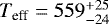 K,
K, 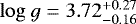 dex, [M∕H] = 0.25 ± 0.14 dex,
 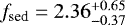 , and
, and 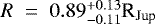 . The solution is in good agreement with the one found with the G statistics when R is constrained. The posteriors on Teff, log g, and fsed are quite similar to those reported in Skemer et al. (2016) using a close MCMC approach and the same model grid. We nonetheless find a lower metallicity. Our value is in excellent agreement with the one determined for GJ 504A. This parameter is correlated with the Teff and R. Skemer et al. (2016) set priors on R corresponding to a range of radii predicted by the “hot-start” evolutionary models. Adopting a flat prior on the radius in the range 0.82–1.26 RJup (see Sect. 5.1.2) does not modify our posteriors significantly. We find
 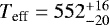 K,
K, 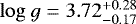 dex,
dex, ![${[M/H]=0.27^{+0.14}_{-0.13}}$](/articles/aa/full_html/2018/10/aa32942-18/aa32942-18-eq28.png) dex,
dex, 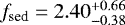 , and
, and 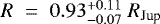 . The analysis does not alleviate the correlation between the fsed and log g values. The radius is more consistent with those of old brown dwarfs. The luminosity is in good agreement with the one determined empirically.
The BACON code used in Samland et al. (2017) couples the petitCODE grids of models to emcee. BACON has been validated on the benchmark T-type companions Gl 570D and HD 3651B (Samland et al. 2017). We used it on GJ 504b photometry. The posterior distributions are shown in Fig. 9 and confirm the fitting solutions with the G statistics when R is unconstrained. However, most of the solutions are found for unphysical radii which are highly correlated to Teff. Moreover, the [M∕H] determination is degenerate with the cloud parameters (Kzz and fsed). The posteriors on [M∕H] might be extended to higher values if the grids of models were created for higher Kzz and fsed values, as it is the case (for fsed) in the Morley grid. The upper limits were not taken into account in the fit.
GJ 504A has a C/O ratio7 of  , close to the value for the Sun (C∕O⊙ = 0.55 ± 0.10; Caffau et al. 2008; Asplund et al. 2009). The atmospheric models used for GJ 504b assume a solar C/O value. Nevertheless, this might not be the case if GJ 504b formed in a disk (see Öberg et al. 2011; Öberg & Bergin 2016). In such a case, one needs to investigate how a different C/O ratio could bias the atmospheric parameter determination. Atmospheric retrieval is a powerful method to estimate the abundances of individual molecules carrying C and O. We attempted a retrieval of the abundances of H2O, CO2, CO, and CH4 with the HELIOS-R (Lavie et al. 2017) and NEMESIS (Irwin et al. 2008) codes. We obtained flat distributions because of the limited number of photometric data points used as inputs and the uncertainties on the data.
We then considered a grid of forward cloud-free models (see Appendix D for the details) exploring different C/O ratios in addition to Teff, log g, [M∕H], Kzz, and R. We used the MULTINEST Bayesian inference tool (Feroz et al. 2009) which implements the Nested Sampling method (Skilling 2006). MULTINEST allows for an efficient sampling of multimodal posterior distributions and avoids the convergence issues that can arise in MCMC runs. The upper limits were taken into account using the method of Sawicki (2012). We report the posterior distributions in Fig. 10 and the best-fitting spectrum in Fig. 11. The posteriors yield constraints on the Teff and log g values which are compatible with those inferred from the model grids not accounting for nonsolar C/O. The metallicity distribution points toward values compatible with those reported in Skemer et al. (2016). The C/O ratio is below solar (C/O =  ) and not correlated with the [M∕H] value. However, we find a strong correlation with the Kzz values which is loosely constrained, but points toward lower values than those inferred with other atmospheric models. We refrained from using the C/O ratio value to discuss the formation mode of GJ 504b since our estimate does not account for possible model-to-model uncertainties.
In summary, the Bayesian analysis confirms the Teff = 550 ± 50 K found in Sect. 5.1.2. We adopt this value in the following analysis. We do not reproduce the posterior distribution on [M∕H] found by Skemer et al. (2016) with the full set of photometric points, or restraining the fit to the subset of data used in Skemer et al. (2016). The metallicity determination is limited by model-to-model systematic error and degeneracies with the cloud properties and log g. The different [M∕H] values may be due in part to the prior choices and the reference solar abundances considered in each model8 and/or to the way the clouds are handled. The posteriors points toward a low surface gravity in agreement with the young-age scenario. Nevertheless, the log g determination is degenerate with [M∕H] and the cloud properties (for models with clouds). The C/O ratio can be determined accurately for cold objects such as GJ 504b using the forward modeling approach. It does not seem to affect the other parameter determination considered for the demonstration ([M∕H], log g, Teff). However, a more robust determination could be achieved with additional datapoints (or spectra) and better accounting for model-to-model uncertainties.
We adopt a log(L∕L⊙) = −6.15 ± 0.15 for GJ 504b based on the values derived from the empirical analysis and confirmed by various modelings with synthetic spectra. Both the Teff and luminosity estimates are in good agreement with those of T8-T9.5 dwarfs (Fig. 12).
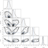 |
Fig. 8 Posterior distributions for GJ 504b atmospheric parameters when the Morley models are considered. |
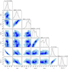 |
Fig. 10 Posterior distribution of atmospheric parameters corresponding to the forward modeling of GJ 504b photometry with cloud-free models exploring different C/O ratios. |
 |
Fig. 11 Best-fitting spectrum found with the forward modeling of GJ 504b SED with cloud-free models exploring the effect of different C/O ratios. |
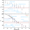 |
Fig. 12 Comparison of the final Teff and bolometric luminosity of GJ 504b (dashed zone) to those of late-T and early-Y dwarfs. The bolometric luminosity values are taken from Dupuy & Kraus (2013) and Delorme et al. (2017a). The temperatures and luminosity of benchmark companions are taken from Table A.2. We added the Teff determined by Leggett et al. (2017), Line et al. (2017), and Schneider et al. (2015) using atmospheric models and report the Teff /spectral type conversion scale of Filippazzo et al. (2015). |
6 Mass estimates
Table 7 reports the masses predicted by the “hot-start” COND models (Baraffe et al. 2003). The masses predicted from the temperature and luminosity agree with each other. The object falls onto the 4 Gyr isochrone in Fig. 13. The 20 Myr isochrone is marginally consistent with the object properties. Conversely, the predicted surface gravities at 21 Myr are in better agreement with those found with the BT-SETTL, petitCODE, ATMO, and Morley atmosphericmodels, but this parameter can be affected by the degeneracies of the atmospheric model fits discussed above.
We also report the “hot-start” model predictions for the Saumon & Marley (2008) models which account for metal-enriched atmospheresas boundary conditions. The predictions are consistent with those of the COND models for the old age range9.
If GJ 504 is a 21 Myr-old system, the mass predicted by the evolutionary models should be sensitive to the way the companion accreted its forming material (Marley et al. 2007) and to the amount of heavy elements it contains (Mordasini 2013). We show in Fig. 14 the joint constraints on the mass and the initial entropy Sinit of GJ 504b imposed by the bolometric luminosity for an age of 21 ± 2 Myr (cf. Marleau & Cumming 2014).
We find that from the luminosity measurement alone, a wide range of masses is possible, from 0.7 MJup upwards. If we truncate the posterior distribution at 2.5 MJup, we obtain a marginalized 68.3% confidence interval on the mass of  and
and  at 90%. Clearly, higher masses than what is shown here would be found to be consistent with the measurement if the Spiegel & Burrows (2012) grid went down to lower initial entropies. The locus of possible M–Sinit combinations can however be compared to planet population synthesis predictions to derive tighter constraints on both mass and post-formation entropy. While in our core-accretion models no planets are found at the same location in the a–M plane as GJ 504b (see Fig. 23 and Sect. 8.3), the M–Sinit relation (with its scatter) is relatively universal. We verified this by comparing the output of the population syntheses of Mordasini et al. (2017), computed for a solar-mass star, to simulations with stellar masses of 1.5 and 2 M⊙ and different migration and planetary growth prescriptions, resulting in very different final a–M distributions; the M–Sinit relation in all cases was similar, only with varying amounts of scatter in Sinit at a given planetmass, which in turn reflects the physics of the core growth.
Comparing the two sets of points in Fig. 14 (inferred from data and predicted from formation models), it is clear that if GJ 504b formed through standard core accretion as represented by the “cold nominal” population of Mordasini et al. (2017), its post-formation entropy is 8.7–8.6 < Sinit < 9.6–9.8 in units of kB∕baryon, with the bounds slightly depending on the stellar mass (from low to high, respectively). This a priori on Sinit leads to M = 1.3 ± 0.4 MJup.
“Hot-start” evolutionary model predictions.
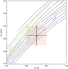 |
Fig. 13 Luminosity and Teff of GJ 504b compared to the COND03 (“hot-start”) evolutionary tracks. The solid lines correspond to the 5,10, 20, 100, 300, 600 Myr and 1, 2, 4, 6, and 10 Gyr isochrones (from top to bottom). The dashed lines correspond to the model predictions for masses of 1, 5, 10, 15, 20, 30, and 40 MJup (from top tobottom). |
 |
Fig. 14 Constraints on the mass and post-formation entropy Sinit of GJ 504b for a (cooling) age tcool = 21 ± 2 Myr. The concave swarm of black points (small open circles) shows all combinations consistent with the luminosity measurement of log L∕L⊙ = −6.15, following the approach described in detail in Marleau & Cumming (2014) but with an MCMC as in Bonnefoy et al. (2014b,c) and using the Spiegel & Burrows (2012) models. The band of colored symbols (filled pentagons) displays the entropy at the time of disk dispersal for the cold nominal populationof Mordasini et al. (2017), that is, assuming full radiative losses at the shock but taking the core-mass effect (Mordasini 2013) into account. The logarithmic colorscale indicates the core mass Mcore. Shown are also the results of Mordasini (2013) for core masses of 20, 33, and 49 MEarth (large open circles connected by lines; bottom to top). The curve at the bottom of the plot is the marginalized posterior on the mass for all small black M–Sinit points (without taking the synthesis results into account). |
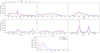 |
Fig. 15 Posterior distributions on the orbital parameters of GJ 504b using all the astrometric epochs as input (in red) or the SPHERE epochs only (in blue). |
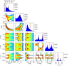 |
Fig. 16 Posteriors on the orbital elements of GJ 504b when considering the astrometry from 2011 to 2017. The red lines and dots depict the best fitting orbit (better χ2). The color scale is logarithmic, blue corresponds to 1 orbit and red to 1000. |
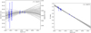 |
Fig. 17 Sample of 100 orbits obtained with the MCMC algorithm applied to GJ 504b astrometry (blue points). |
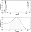 |
Fig. 18 Fromtop to bottom panels: line-of-sight inclination i⋆ of GJ 504, and absolute difference between ic and i⋆ when only i⋆≥ 90° are considered. The dashed zones correspond to 68.28% of the solutions. |
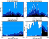 |
Fig. 19 Companion detection probability (white text and isocontours) when combining the sensitivity maps of multiple epochs of imaging data and the Lick or SOPHIE radial velocities of GJ 504A for the two possible age ranges for the system. |
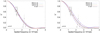 |
Fig. 20 Theoretical squared visibilities of a star without a spot (solid black line), and of a star with a spot (ws) as modelised with COMETS (Ligi et al. 2015). The different solid color lines represent the squared visibilities at different wavelengths and positions. The black circles represent the actual interferometric measurements (with error bars) of GJ504 performed with VEGA/CHARA. Left panel: a spot with a filling factor p = 7%. Right panel: the same but for p = 22%. |
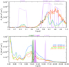 |
Fig. 21 Predicted apparent fluxes of GJ 504b in the near- and mid-infrared corresponding to the best-fitting synthetic spectra found in Sect. 5 with the G statistics and some knowledge of the object radius. The transmission of some key filters of JWST instruments are overlaid. We report the L-band photometry (Subaru/IRCS, LBTI/LMIRcam) of GJ 504b (black). |
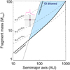 |
Fig. 22 Gravitational instability model adapted to the case of GJ 504. Fragments are allowed to form if they respect the Toomre andcooling criteria. GJ 504b properties are reported. The pink curve corresponds to the posterior distribution of the companion semi-major axis found with our MCMC orbit-fitting package (Sect. 7.1). The dashed lines correspond to the disk mass distribution for a different hypothesis on the initial disk mass. |
 |
Fig. 23 Population synthesis at 20 Myr for core-accretion models including Type I and II migration and dynamical scattering between multiple planet embryos in the disk. We considered the case of 1, 1.5, and 2 M⊙ central stars. The color shows the enrichment relative to the star. |
7 Architecture
7.1 Companion orbit
We considered the astrometry reported in Table 2 as input of our MCMC orbit fitting packages to set constraints on the orbital parameters of GJ 504b. The code was developed for β Pictoris b and Fomalhaut b’s orbits (Chauvin et al. 2012). We considered a mass of 1.2 M⊙ for GJ 504A. We assume flat priors on log(P), e, cos(i), Ω + ω, ω − Ω, and Tp following Ford (2006). We ran ten chains in parallel and used the Gelman-Rubin statistics as convergence criterion (see details in Ford 2006).
The fit was performed on the whole set of epochs. We neglected the epoch from August 15, 2011 reported in Kuzuhara et al. (2013) for which the data were taken under poor conditions and the astrometry appears to be deviant. However, it is still possible that some systematic angular offsets between each instrument could have biased our analysis. We then also modeled the SPHERE epochs only, for comparison. The posteriors are shown in Fig. 15 for the two data sets. Figure 16 shows the correlation between the different posterior distributions of orbital parameters of GJ 504b when all the astrometric epochs are accounted for in the fit.
The posterior distributions do not change significantly when considering the homogeneous SPHERE data, or the data from all instruments. The accuracy of the SPHERE astrometry yields the most constraints on the orbital parameters and is therefore not heavily influenced by putative systematic errors on the HiCIAO and IRCS astrometry. We, therefore, considered the results from the whole set of epochs in the following. A sample of corresponding orbits is shown in Fig. 17. This shows that no curvature can be detected with the present astrometric monitoring.
The posterior on the semi-major axis points at 44 au which corresponds to the companion projected separation with 68% of the solutions in the range 44 ± 11 au. The fit excludes orbits with a semi-major axis shorter than ~27.8 au. The periods are significantly longer than the time span of the Lick and SOPHIE radial velocities and are likely to prevent us from obtaining constraints on the dynamical mass of GJ 504b.
The eccentricity is lower than 0.55 and peaks at 0.31 (e = 0.31 ± 0.15; 68% solutions). Our new data and fit do not yield solutions at higher eccentricity found by Kuzuhara et al. (2013). We find an inclination of  degrees. There is no solution for i < 120° as found by Kuzuhara et al. (2013)10, but that might be related to our priors which favor small semi-major axis and large inclinations.
We ran the same analysis considering masses of 1.10 and 1.25 M⊙ for GJ 504A. The posteriors are marginally affected by this change.
7.2 A spin-orbit misalignment?
The radius R⋆ of GJ 504A determined in Sect. 2.3 can be used to derive the line-of-sight inclination of the star i⋆ following:
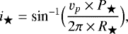 (3)
(3)
where vp = v ⋅sin i and P⋆ is the rotation period. We measure vp = 6.5 ± 1.0 km s−1 from the setof SOPHIE data. This value is consistent with the one reported in D’Orazi et al. (2017b). We used  (Donahue et al. 1996)
We considered Gaussian distributions on each measurement to find a resulting probability ditribution corresponding to 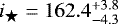 degrees or
  degrees. The two values are due to the [0, π] degeneracy of the sin function.
The posterior on the orbit inclination ic of GJ 504b inferred from the MCMC analysis (Sect. 7.1) can be used to derive the relative orientation of the stellar spin axis and orbital angular momentum vector φ, or true obliquity:
 (4)
(4)
where λ is the projected obliquity11. In our case, λ is unknown, but as explained in Bowler et al. (2017), the lower limit on φ can be inferred from the absolute difference between ic and i⋆: φ ≥Δi ≡|i⋆− ic|. Therefore, a system with a posterior probability function on Δi extending to 0° can still have a non-zero true obliquity, and therefore a spin-orbit misalignment. We show in Fig. 18 the posteriors on i⋆ and Δ i. The probability that Δi is greater than 10° is 78.1%. This probability is conservative given that our priors on the orbit fit of GJ 504b favor large inclinations. In addition, this represents the minimum values of φ in this system. Therefore, GJ 504A and b may have a spin-orbit misalignment. Further astrometric monitoring will help to consolidate this result.
7.3 Constraints on additional companions
The joint use of the radial velocities (RVs) of GJ 504A and contrast limits at each on-sky projected separation inferred from direct imaging data taken at multiple epochs allows limits to be placed on the mass of undetected companions from the star up to semi-major axis corresponding to the field-of-view coverage of the imaging cameras.
The MESS2 Monte Carlo simulation code generates synthetic planet populations and compares their RV signals and projected separation at each epoch to the data (Lannier et al. 2017) to evaluate detection probabilities. We applied MESS2 to RV data obtained with SOPHIE (listed in Appendix E) and at the Lick Observatory independently. Potential offsets between the two sets of data may indeed exist because of the different methods used to derive the RVs.
We used the local power analysis (LPA; Meunier et al. 2012) to interpret these RV data. The LPA method generates periodograms of RV time series for each synthetic planet and compares them to the periodogram of the observed RV data within given orbital periods. We used the IRDIS detection limits obtained from May 2015 to February 2017 that we converted to masses, and those derived from the IFS data from March 2016 and June 2015. We considered, in addition, the detection limits inferred from the HiCIAO and IRCS data obtained as part of the SEEDS survey (March 26 and May 22, 2011; April 12 and May 25, 2012 data) and reprocessed for this study using the ACORNS pipeline (Brandt et al. 2013). Those datasets allow for an improved coverage of the orbit of putative companions. All the detection limits inferred from the imaging data assume “hot-start” formation conditions (Baraffe et al. 2003). The predictions should indeed not be heavily sensitive to the initial conditions at an age of 4 Gyr. In addition, the difference in luminosity predictions between the “hot” and “cold” stars tends to decrease with the planet mass.
The detection probability curves inferred from the Lick and imaging data are shown in Fig. 19 for the two isochronal age ranges of GJ 504A. When considering the old isochronal age, 90% of the objects more massive than 30 MJup would have been detected from 0.01 to 80 au. MESS2 does not presently enable simulation of the RV signals of planets whose semi-period exceeds the time span of the data. This explains the sudden loss of sensitivity at ~15 au. An upgrade of MESS2 would allow us, in the near-future, to handle non-detection of planets with longer periods than those set by this observation threshold.
No object more massive than 2.5 MJup (apart GJ 504b) exists in the system assuming the young isochronal age. Our simulations reveal in addition that the Lick data (21.6 yr span) enable a more in-depth exploration of the separations from 0.2 to 6 au than the SOPHIE data (3.2 yr span). Both of the data sets give comparable constraints from 0.01 to 0.1 au.
8 Discussion
8.1 Conflicting age indicators
8.1.1 The planet engulfment scenario
Fuhrmann & Chini (2015) proposed that the engulfment of a jovian planet (2.7 MJup) could have sped up GJ 504A’s rotation velocity. D’Orazi et al. (2017b) estimate that the engulfment should have occurred no more than 200 Myr ago for the system to keep a sufficient imprint of the event on the star rotation speed. Such an engulfment may also enrich the host star in metals (Carlberg et al. 2012; Saffe et al. 2017).
In that case, what could have triggered the engulfment long after the dispersal of the circumstellar disk? Our detection limits indicate that no other companions more massive than the proposed engulfed planet are presently located in the first astronomical unit around GJ 504A. GJ 504b is likely the most massive object in the system, and therefore a good candidate perturber. The Lidov–Kozai mechanism (Kozai 1962; Lidov 1962) invoked by Fuhrmann & Chini (2015) and D’Orazi et al. (2017b) could only operate in the system if the obliquity φ of GJ 504b were higher than at least 40 deg. Additional astrometric monitoring of the companion is required to carve the distribution of relative inclinations Δ i and provide a lower limit on φ. Two known systems have recently been discovered with close-in low-mass planets on eccentric orbits and more massive companions on wide-orbits: HD 219828 (Santos et al. 2016) and HD 4113 (Cheetham et al. 2018a). These systems might then be good proxies of the architecture of the GJ 504 system prior to the putative engulfment.
8.1.2 Effect of polar spots
Because GJ 504A is active and seen close to pole-on, high-latitude spots may be affecting the luminosity and Teff estimates used for comparison to the tracks. These spots are predicted to occur on rapid rotators such as GJ 504A and young stars (Schuessler & Solanki 1992; Buzasi 1997; Schrijver & Title 2001; Holzwarth et al. 2006; Yadav et al. 2015). Observations of polar spots on active G-type stars might have been observed (e.g., Marsden et al. 2005, 2006, 2011; Waite et al. 2011, 2017). The polar spots (or cap) can fill up to 50% of the stellar surface and have lifetimes of about a decade. Given a spot filling factor p (defined as  , where Rs is the spot radius), the observed luminosity Lobs of GJ 504A relative to the photosphere luminosity Lphot is
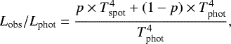 (5)
(5)
where Tspot is the spot temperatureand Tphot the photosphere temperature.
The disk-averaged temperature measurement Tobs can be influenced by spots in a similar way:
 (6)
(6)
We used the SAFIR simulator described in Desort et al. (2007) to evaluate the filling factor and inclination of a putative long-lived spot responsible for the RV variations measured with SOPHIE. Assuming a 1.2 M⊙, 1.3 R⊙ 6205 K star inclined by ~17 degrees with respect to edge-on, the observed amplitude of the variations can be reproduced with a 2000 K cooler dark spot (Berdyugina 2005) inclined by 5 degrees with respect to the spin axis and covering p ~ 6% of the star surface.
The PARSEC evolutionary models indicate that the age predictions should be more sensitive to a bias on the Teff measurement. We find that a spot with only p = 7% would lower the Teff determination by 150 K and lead to intermediate ages in marginal agreement with the upper limits derived from the gyrochronology (up to 220 Myr) if we assume that the luminosity is not affected by spots at the time of measurements. Conversely, p = 22% would be required to sufficiently bias the isochronal age based on the luminosity estimate. The data used to compute the luminosity of GJ 504A (Appendix A) were taken on individual nights from 1980 to 2014. Such a large spot would have implied Teff differences of 440 K at least which would have been noticed in the star’s SED fit. Therefore, we are confident in the isochronal age derived from the luminosity.
Spots may explain in part the ~200 K scatter on the Teff values found in the literature (see Table 2 of D’Orazi et al. 2017b) and the slight difference on the old isochronal age range ( Gyr) that can be inferred from the Teff value of D’Orazi et al. (2017b) and the interferometric radius. However, the Teff value derived in D’Orazi et al. (2017b) is one of the highest reported in the literature; furthermore, it is inferred from the excitation balance of 100 Fe lines which form at different optical depths within the star’s photosphere. The lack of a significant scatter in the abundances derived from the individual lines suggests that spots have not significantly biased the Teff determination at the time of the observations.
Stellar activity is also known to influence the interferometric observables (see, Chiavassa et al. 2014; Ligi 2014; Ligi et al. 2015). We have therefore verified whether a spot could have biased our visibility measurements using the COMETS code (Ligi et al. 2015) to model the visibility of a star with a spot at its surface. We considered two filling factors p = 7% and p = 22% and a spot temperature of 4205 K, as above. Spots were placed at the edge of the stellar disk, with position angles ranging from 0 to 2π with π∕4 increments (that is, all around the stellar disk). Due to symmetry effects, this leads to only three different visibility curves. The visibilities were computed for the three different wavelengths (550, 710, and 730 nm) used for measuring the angular size of GJ 504A.
Figure 20 shows the squared visibilities measured with VEGA/CHARA (black circles), that led to an angular diameter of 0.71 mas. The solid black line represents the fit corresponding to this angular diameter (with a limb-darkened model as explained in Sect. 2.3). The different colored curves represent the theoretical visibilities of a star with a spot as modeled with COMETS at the different wavelengths and positions tested.
We find that a spot with p = 7 or 22% induces a change in the visibility curve which is still within the dispersion of measured values. Therefore, spots such as those considered here are not likely to have significantly biased GJ 504A’s angular diameter measurement.
We, therefore, conclude that while spots may indeed be affecting the RVs, luminosity, radius, and Teff estimates of GJ 504A, their effect is unlikely to bias all those quantities together by sufficient amounts and change the isochronal age estimates of the star.
8.2 Disentangling the atmospheric model solutions
We show in Fig. 21 the synthetic spectra in the L-M band and in the mid-infrared corresponding to the models fitting the presently available photometry of GJ 504b (Table 6; solutions with some pre-requisite on the companion radius). The ATMO and Exo-REM models predict very similar spectra distinctive from those corresponding to the Morley and petitCODE solutions. The difference arises from the non-equilibrium chemistry which is not considered in the case of the two latter models and modulates the strength of the CO2 and CO absorption bands centered around 4.3 and 4.7 μm, respectively.Adaptive-optics M-band imaging from the ground should already tell whether the non-equilibrium chemistry is a pre-requisitefor modeling the companion emission flux (model-to-model contrast between 1.16 and 1.48 mag in the M-band filter of the VLT/NaCo instrument). Coronographic imaging with the F430M and F460M filters of the Near Infrared Camera (NIRCam) on the James Webb Space Telescope (JWST) should also better constrain the shape of the 3.7–5 μm pseudo-continuum and could disentangle the ATMO and Exo-REM solutions.
Observations at longer wavelengths will be a niche for the Mid-Infrared Instrument (MIRI) of JWST. We can estimate that the contrast between GJ 504b and GJ 504A should range between 4 × 10⁻⁶ and 2.5 × 10⁻⁴ from 5 to 28.5 μm using the set of atmospheric models considered above and the SED of GJ 504A (Appendix A). The use of the four-quadrant phase masks together with ADI will be mandatory to reach GJ 504b contrasts and avoid saturation (Boccaletti et al. 2015). The four-quadrant phase masks can only be used jointly with the F1065C (λc = 10.575 μm, Δλ = 0.75 μm), F1140C (λc = 11.40 μm, Δλ = 0.80 μm), and F1550C (λc = 15.50 μm, Δλ = 0.90 μm) filters. The MIRI photometry should enable to distinguish between the ATMO and Exo-REM solutions. The Exo-REM models indicate that the spectral slope between 11 and 15 μm probed by the F1140C- F1550C color should also be a good indicator of the percentage of the disk surface covered by clouds.
To conclude, we considered two representative solutions probing the log g/[M∕H] degeneracy in the posterior distributions shown in Figs. 8 and 9 at Teff = 550 K. The spectra indicate that narrow and broad band photometry with JWST longward of 3 μm should not break the log g/[M∕H] degeneracy for all but the ATMO solutions. The MIRI data coupled to the SPHERE data points should nonetheless set stringent constraints (< 100 K) on the Teff based on our simulations and should allow for reduction of the error bar on the luminosity. The comparison of that Teff and luminosity to evolutionary tracks (Fig. 13) is a way to investigate the system age independently from GJ 504A.
8.3 Formation pathway
If confirmed, a spin-orbit misalignment of GJ 504b (Sect. 7.2) would be a remarkable property of the system, in particular with respect to the solar system planets. Such misaligments are indirectly observed on protostar pairs (e.g., Offner et al. 2016; Brinch et al. 2016) and are consistent with a stellar-like formation scenario (e.g., Boss & Bodenheimer 1979). Spin-orbit misalignments are also clearly established for close-in planets with orbital periods ranging from 0.73 (55 Cnc e; Bourrier & Hébrard 2014) to 207.6 days (Kepler-462 c; Ahlers et al. 2015). Dynamical interaction between planets is a possible cause of those misalignments (e.g., Chatterjee et al. 2008), but other processes such as the magnetic interaction between the inner disk and the star (Lai et al. 2011; Spalding & Batygin 2014) or disk-warping (e.g., Terquem 2013) have also been proposed. Bowler et al. (2017) reported a likely nonzero obliquity for the ROXs 12 system composed of a 17.5 ± 1.5 MJup companion (“hot-star” mass) at a projected separation of 240 au from a low-mass (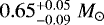 ) young (
 Myr) star. This is to our knowledge the only other measurement of the obliquity of a wide-orbit (>10 au) companion less massive than 30 MJup. Bowler et al. (2017) also show that this system has a tertiary stellar component at a projected separation of 5100 au, which makes the system’s architecture different from that of GJ 504. Some other properties of the GJ 504 system may also be informative. The companion is in a mass range either below, or right inside the so-called “brown-dwarf desert” observed at short separations for solar-type stars (e.g., Sahlmann et al. 2011; Ma & Ge 2014) and likely existing at larger separations (Reggiani et al. 2016). The companion mass ratio q with GJ 504A is
  % or
% or  %, depending on the isochronal age range considered. If the system is 4 Gyr old, GJ 504b still belongs to a very short list of objects resolved at projected separations smaller than 50 au (HD 206893, HR 2562B, HIP 73990B & C; Hinkley et al. 2015b; Milli et al. 2017; Delorme et al. 2017c; Mesa et al. 2018) with such extreme q values. All those companions are found around debris disk stars. GJ 504b’s semi-major axis is probably lower than 200 au in contrast to the 20–30 MJup G-type star companions (e.g., HN Peg b, HD 203030B; Metchev & Hillenbrand 2006; Luhman et al. 2007) found at large (>500 au) projected separations; e.g., beyond the typical size of circumstellar disks of T-Tauri stars (e.g., Piétu et al. 2014; Tazzari et al. 2017; Tripathi et al. 2017).
If GJ 504b is a 14–33 MJup object, its orbital properties and mass ratio should still be compatible with a stellar-like formation mechanism (e.g., Lodato et al. 2005). Metchev & Hillenbrand (2009) argue that the companion mass function follows the same universal form over the entire range between 0 and 1590 au in orbital semimajor axis. They predict a peak in semi-major axes for brown dwarfs at ~30 au which is broadly compatible with the present constraints on the semi-major axis of GJ 504b. Most orbital solutions of GJ 504b also correspond to periods close to the most frequent values found for solar-type star binaries (P = 293.6 days; see Fig. 13 of Raghavan et al. 2010).
We also investigated whether the companion could have formed in a disk. We generated a disk instability model (Klahr et al., in prep.; seealso Janson et al. 2011) adapted to the case of GJ 504 (stellar luminosity and metallicity). The model predicts the range of semi-major axis and clump masses allowed to form and cool down more rapidly than the local Keplerian timescale in Toomre-unstable disks (Toomre 1981). The result is shown in Fig. 22. Clumps with masses in agreement with the companion properties can form if we adopt the old isochronal age for the system. However, the allowed fragmentation zone is predicted to be at larger semi-major axis than most solutions found from the MCMC orbital fits. This can be explained if the disk opacity is lowered, and therefore not scaled on the stellar metallicity (this would be the case if GJ 504A was initially a solar-metallicity star that was later enriched by a planet engulfment event; see Sect. 8.1). In such a case, clumps can cool down sufficiently rapidly at shorter separations. The companion may have alternatively been formed at larger separation subsequently undergoing inward disk-induced migration (for instance through the Type II process which allows for clump survival; Stamatellos 2015; Nayakshin 2017). This formation at a wider distance would also allow for a lower disk mass.
The model cannot account for GJ 504b if it is a  21 Myr-old planet. However, more complex models allowing for a more detailed investigation of the free parameters in the GI models (e.g., Boss 2017) and subsequent planet embryo evolution (protoplanet migration, clump–clump dynamical interactions, “tidal downsizing”, etc.; e.g., Forgan & Rice 2013; Hall et al. 2017; Müller et al. 2018) may lead to different conclusions.
We compare GJ504b to the Bern core-accretion population synthesis results in Fig. 23. The model considers the formation of multiple planet embryos per disk (50, 20, and 10 embryos per disk for the simulations with 1, 1.5, and 2 M⊙ central objects, respectively) and Type I and II migration (Alibert et al. 2005; Mordasini et al. 2012; Alibert et al. 2013). The bulk enrichment in solids of each final planet is reported in the figure. With a lower limit of 27.8 au on its semi-major axis, GJ 504b appears as an outlier of the population for the two possible age ranges. The models can however still form a few objects as massive and distant as the companion. The simulations indicate that all planets more massive than 10 MJup should not be significantly metal-enriched with respect to their host stars. This is in good agreement with the atmospheric metallicity found with the Morley and petitCODE models and the MCMC method.
8.4 Finding analogs of GJ 504b with VLT/SPHERE
Most of the SHINE observations are performed with the IRDIFS mode of the instrument. The H-band observations ensure good AO performance, an optimal use of the apodized Lyot coronograph, and low background emission. The IFS can distinguish cool companions in the first 0.8–1.2′′ from hotter background objects through the detection of characteristic spectral features. That is also one of the best characterized modes for the astrometric monitoring. The unusual colors of GJ 504b call however for a re-investigation of the detection capabilities of ultracool companions with the various instrument modes of SPHERE.
We estimated the absolute magnitude and colors12 of planets and brown dwarfs for three characteristic ages in the field pass-bands using the Exo-REM atmospheric models as boundary conditions (see Appendix F).
The Exo-REM models predict a strong sensitivity of the absolute magnitudes to the cloud coverage and metallicity, in particular for the lowest masses (and Teff). The modelsalso show that the companions have a higher or similar brightness in the J3 filter. This adds to the fact that the typical stars observed with SPHERE have J-H > 0 or J-K > 0, therefore leading to more favorable predicted contrasts at J3. In some cases, DBI imaging with the J2J3 filter could therefore become advantageous for the detection of cool companions. This can be illustrated when considering the G0 star HIP 19148. The star is a member of the 625 Myr-old metal-enriched Hyades cluster (de Bruijne et al. 2001). Using the ESO exposure time calculator13 (version P101.3), we could generate contrast curves for the J2J3 and H2H3 bands considering median observing conditions (seeing of 0.8–1.0′′), 64 s exposures to minimize the read-out noise, and the ADI performance reached during a 1.5 h sequence of coronographic exposures. We used the 2MASS J and H magnitudes and the Gaia-DR1 distance (Gaia Collaboration 2016) to compute the sensitivity and compare it to the predicted magnitudes of 5, 8, and 15 MJup objects. The simulation predicts that we would miss a 8 MJup object in the H2 band at the physical projected separation of GJ 504b while it would be comfortably detected in the J3 channel, in particular if the object is metal- enriched.
The J2J3 mode offers a second advantage. Observations of stars in the galactic plane usually lead to the detection of numerous background stars with IRDIS. When reported in color-magnitude diagrams and assuming they are at the same distance of the target, those point sources line up and form a locus. This locus has the same colors as K and early M stars but is spread in luminosity and does not necessarily share the same colors as cool companions. Therefore, the placement of candidate point sources into those diagrams offers a simple way to disentangle background stars from bound companions. When considering the H2H3 mode, the locus intersects the sequence of cool objects at the L/T transition (where companions such as HN Peg b or HR8799bcde lies) and falls close to the sequence of late-M dwarfs (Langlois et al., in prep.). It is therefore not always possible to determine whether the object is a background star or a substellar companion. We build up in Fig. 24 a locus of contaminants from the J2J3 observations of HIP 67497, HD 115600, and HIP 92984 obtained as part of SHINE (SHINE collaboration, priv. comm.). The point sources draw a locus distinct from the sequence of young and old late-M, L, and T dwarfs. The faintest contaminants have a 1.5 mag color difference with known Y dwarfs. Their colors follow the interstellar reddenning vector. Cool companions such as GJ 758b or GJ 504b would easily be identified from the method. Dusty L-type planets such as HIP 65426b would also be discriminated from the locus of contaminants. Therefore, DBI observations with the J2J3 filters may not necessarily require a follow-up to confirm that the point sources do not share the target proper motion.
 |
Fig. 24 Color-magnitude diagram exploiting the J2 and J3 photometry of SPHERE. We report the photometry of candidate companions detected around three SHINE targets with the DB_J23 filter of IRDIS (grey stars symbols). The reddening vector of 0.5 μm forsterite grains and the one corresponding to the interstellar extinction are overlaid (see Bonnefoy et al. 2016, for the details on how the vectors are computed). |
9 Conclusion
Because it is a nearby bright star, GJ 504 can be observed with a variety of techniques. This work presents new interferometric, radial-velocity, and high-contrast imaging observations that shed a new light on the system. Two isochronal age ranges (21 ± 2 Myr and 4.0 ± 1.8 Gyr) are compatible with the interferometric radius of GJ 504A. The conflicting conclusions from the various alternative age indicators do not allow usto firmly choose one age or the other. The known companion is a T8-T9.5 object with a peculiar SED from 1 to 2.5 μm. The SED is compatible with a low surface gravity and/or super-solar metallicity atmosphere. The metallicity determination is limited by systematic errors between atmospheric models and degeneracies with the surface gravity. Ouranalysis also reveals that the metallicity is not degenerate with the carbon-to-oxygen ratio. The surface gravity is consistent with the young isochronal age of the system. We estimate a mass of 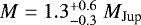 and
and 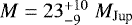 for GJ 504b forthe young and old isochronal system ages, respectively. These masses account for a wide range of plausible initial conditions and rely on the bolometric luminosity inferred independently from the empirical and atmospheric model analysis of the companion SED. The orbit of GJ 504b has a semi-major axis larger than 27.8 au, an eccentricity lower than 0.55, and an inclination in the range (125–180) degrees. The interferometric radius of thestar and its v sin i allows determinations of the line-of-sight inclination. A comparison with the inclination of the orbit of GJ 504b suggests that the system could have aspin-orbit misalignment. The radial velocity and imaging data allow exclusion of companions more massive than 2.5 and 30 MJup from 0.01 to 80 au assuming the young and old age range, respectively.
If GJ 504b is a brown-dwarf in an old system, we show that gravitational instability models possibly coupled to inward migration might explain its properties. Population synthesis models confirm that the core-accretion models can form such a massive object, but preferentially at semi-major axis shorter than 30 au. Both formation models would be challenged if the object is a planet with  .
.
Additional key measurements could be obtained in the near future to better constrain the origins of the GJ 504 system. Additional astrometric monitoring of GJ 504b is crucially needed to (1) tighten down the posteriors on the inclination of GJ 504b orbit and confirm the spin-axis misaligment, and (2) constrain better the eccentricity. The latter could be related to the formation mechanism (see Ma & Ge 2014). JWST photometry and spectra of GJ 504b should yield the first robust constraints on the C/O, O/H, and C/H (or metallicity) ratios and on the importance of nonequilibrium chemistry in the atmosphere of GJ 504b. It will then become possible to compare the abundances to those of brown dwarfs (Line et al. 2017) and planets (e.g. Benneke 2015; Lavie et al. 2017). Deeper imaging data as gathered with the JWST should set stringent constraints on the probability of detection of companions beyond 80 au. Conversely, additional monitoring with SPHERE may carve the planet detection probability parameter space in the (15–30) au range where companions slightly more massive than GJ 504b may still reside if the system is old. Asteroseismology of the host star might enable us to close the debate on the system age. The more accurate luminosity and surface gravity of GJ 504b gathered by JWST might also enable the two possible isochronal ages for the system to be disentangled. Gaia may detect the wobble induced by GJ 504b over the duration of its nominal mission (5 yr) which could be used to exclude some of our orbital solutions and set upper limits on the companion mass.
To conclude, the J2J3 DBI filter of SPHERE offers good prospects for the detection and follow-up strategy of analogs of GJ 504b. Direct imaging surveys of nearby metal-rich G-type stars using this pair of filters would be of value to constrain the formation models.
Acknowledgements
The authors thank the ESO staff, the CHARA team, and the VEGA team for support in conducting the observations. M.B. is grateful to B. Burningham, G. Mace, D. Cushing, M. Liu, R.D. Rosa, D. Lafrenière, D. Kirkpatrick, A. Burgasser, J. Patience, B. Bowler, D. Lachapelle, E. Wright, and S. Leggett for providing the spectra of benchmark objects. We thank K. Rice, D. Forgan, and K. Todorov for fruitful discussions.This research has benefitted from the SpeX Prism Library (and/or SpeX Prism Library Analysis Toolkit), maintained by Adam Burgasser at http://www.browndwarfs.org/spexprism and from the Y Dwarf Compendium maintained by Michael Cushing at https://sites.google.com/view/ydwarfcompendium/. This research has made use of the SIMBAD database and VizieR catalogue access tool (operated at CDS, Strasbourg, France). This research has made use of NASA’s Astrophysics Data System and of the Extrasolar Planet Encyclopedia (http://exoplanet.eu/). Part of the planet population of Fig. 23 is publicly available on DACE, the Data Analysis Centre for Exoplanets of the NCCR PlanetS reachable at https://dace.unige.ch. Additional populations will be added in future. DACE yields both interactive snapshots of the entire population at a given moment in time like the population-wide a–M or M–R diagrams as well as formation tracks of individual planets (e.g., M(t), R(t), etc.) for all synthetic planets. This publication makes use of VOSA, developed under the Spanish Virtual Observatory project supported from the Spanish MICINN through grant AyA2011-24052. This work is partly based on data products produced at the SPHERE Data Centre hosted at OSUG/IPAG, Grenoble. Data analysis was partially carried out on the open use data analysis computer system at the Astronomy Data Center, ADC, of theNational Astronomical Observatory of Japan. SPHERE is an instrument designed and built by a consortium consisting of IPAG (Grenoble, France), MPIA (Heidelberg, Germany), LAM (Marseille, France), LESIA (Paris, France), Laboratoire Lagrange (Nice, France), INAF Osservatorio di Padova (Italy), Observatoire de Genève (Switzerland), ETH Zurich (Switzerland), NOVA (The Netherlands), ONERA (France), and ASTRON (The Netherlands) in collaboration with ESO. SPHERE was funded by ESO, with additional contributions from CNRS (France), MPIA (Germany), INAF (Italy), FINES (Switzerland), and NOVA (The Netherlands). SPHERE also received funding from the European Commission Sixth and Seventh Framework Programmes as part of the Optical Infrared Co-ordination Network for Astronomy (OPTICON) under grant number RII3-Ct- 2004-001566 for FP6 (2004-2008), grant number 226604 for FP7 (2009-2012), and grant number 312430 for FP7 (2013-2016). We also acknowledge financial support from the Programme National de Planétologie (PNP) and the Programme National de Physique Stellaire (PNPS) of CNRS-INSU in France. This work has also been supported by a grant from the French Labex OSUG@2020 (Investissements d’avenir – ANR10 LABX56) and from the Agence Nationale de la Recherche (grant ANR-14-CE33-0018). G.D.M. and C.M. acknowledge the support from the Swiss National Science Foundation under grant BSSGI0_155816 “PlanetsInTime”. Parts of this work have been carried out within the frame of the National Center for Competence in Research PlanetS supported by the SNSF. This work is based upon observations obtained with the Georgia State University Center for High Angular Resolution Astronomy Array at Mount Wilson Observatory. The CHARA Array is supported by the National Science Foundation under Grant No. AST-1211929. J.H. is supported by the Swiss National Science Foundation (SNSF P2GEP2_151842). A.Z. acknowledges support from the CONICYT + PAI/ Convocatoria nacional subvención a la instalación en la academia, convocatoria 2017 + Folio PAI77170087.
Appendix A GJ504A SED and luminosity
The magnitude of GJ 504A is unknown in the SPHERE passband. We, therefore, built a model of the star SED from the Johnson V and B band (Kharchenko et al. 2009), J, H, and K bands (Kidger & Martín-Luis 2003), AKARI S09W and L18W (Ishihara et al. 2010), IRAS 12 μm (Moshir 1989), WISE W3, and W4 (Cutri et al. 2014), and Herschel/PACS 100 μm (Moro-Martín et al. 2015)photometry14. That SED is well reproduced by a BT-NEXTGEN synthetic spectra (Allard et al. 2012b) with Teff = 6200 K, log g = 4.5, and M/H = 0.3. Those parameters are the closest ones of the solution found by D’Orazi et al. (2017b) using high-resolution spectra. We confirm that no excess can be found up to 100 μm with our fitting solution. The flux-calibrated model spectrum reproduces equally well (Fig. A.1) the shape and flux of the STELIB medium-resolution (R ~ 2000) optical spectrum (320–989 nm) of the star (Le Borgne et al. 2003) obtained in April 1994. We collected and averaged archival flux-calibrated UV spectra of the star from the “IUE Newly Extracted Spectra” (INES) database15. The spectrawere collected with the LWR and SWP camera of the International Ultraviolet Explorer (Rodríguez-Pascual et al. 1999; Cassatella et al. 2000; González-Riestra et al. 2000, 2001) and have a reliable flux in the interval 150–331nm. We also reduced data of GJ 504A gathered with the SINFONI NIR integral field spectrograph (Eisenhauer et al. 2003; Bonnet et al. 2004) on June 9, 2014 (PI CACERES; Program 093.C-0500). The data were acquired with the H+K mode of the instrument yielding continuous medium-resolution (R ~ 1500) spectra from 1.45 to 2.45 μm. The SINFONI data were reduced with the ESO data handling pipeline version 3.0.0 through the Reflex environment. Only one datacube, corresponding to a science exposure obtained at 02h41m04s UT, contained the star in the field of view. The star spectrum was extracted over a circular aperture with a radius of 325 mas. The spectrum was corrected from telluric absorption using the observation of the B9V star HD 141327 observed before GJ 504A. The 1.8–1.95 μm range was affected by telluric line residuals and was not considered any further. We flux-calibrated the spectrum using the K band flux from Kidger & Martín-Luis (2003). The H and K-band SINFONIspectrum is well reproduced by the BT-NEXTGEN model (Fig. A.1) and can be used to derive reliable IRDIS magnitudes of GJ 504A in the H2H3 and K1K2 channels (see below). We replaced the BT-NEXTGEN spectrum with the INES, STELLIB, and SINFONI spectra of GJ 504A and integrated the SED to estimate a log L∕L⊙ = 0.35 ± 0.01 dex. The error accounts for an uncertainty of 100 K on the Teff of the BT-NEXTGEN model fit and for the uncertainty on the distance (0.08 pc; van Leeuwen 2007). The value is in good agreement with the one (log L∕L⊙ = 0.35 ± 0.05) derived by Fuhrmann & Chini (2015) from a V -band bolometric correction.
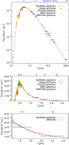 |
Fig. A.1 Photometry of GJ 504A (blue dots) compared to a BT-NEXTGEN synthetic spectrum (red line) at Teff = 6200 K, log g = 4.5, and M/H = +0.3 scaled in flux. The flux-calibrated INES, STELIB, and SINFONI spectra (yellow, green, and grey lines, respectively) of the star are compatible with the flux-calibrated model-spectrum. |
We used the spectrum of GJ 504A considered for the bolometric luminosity estimate and a spectrum ofVega (Mountain et al. 1985; Hayes 1985) to compute the photometric shifts between the J, H, and K photometry of GJ 504A and the SPHERE DBI filters of IRDIS. We also re-derived the CH4S and CH4L photometry of GJ 504A from the published H-band magnitude, taking into account the SINFONI spectrum of the star. The resulting magnitudes for GJ 504A are reported in Table A.1.
Apparent magnitude of GJ 504A in the IRDIS and HiCIAO CH4 filters.
Properties of late-T benchmark companions and peculiar isolated objects.
Appendix B Benchmark late-T objects
We report in Table A.2 the properties of the benchmark late-T companions mentioned in Sect. 4.
Appendix C Details on the color–magnitude and color–color diagrams
This appendix describes the way the color-magnitude and color-diagrams shown in Sect. 4 are built.
We used spectra of M, L, and T dwarfs from the SpeXPrism library (Burgasser 2014) and from Leggett et al. (2000) and Schneider et al. (2015) to generate synthetic photometry in the SPHERE filter passbands. The zero points were computed using a flux-calibrated spectrum of Vega (Hayes 1985; Mountain et al. 1985). We also considered the spectra of young and/or dusty free-floating objects from Liu et al. (2013), Mace et al. (2013a), Gizis et al. (2015), and of young companions (Patience et al. 2010; Lafrenière et al. 2010; Wahhaj et al. 2011; De Rosa et al. 2014; Bailey et al. 2014; Bonnefoy et al. 2014a; Gauza et al. 2015; Lachapelle et al. 2015; Stone et al. 2016; Rajan et al. 2017). The colors and absolute fluxes of the benchmark companions and isolated T-type objects are generated from the distance and spectra of those objects (See Appendix A.2 for the details.). To conclude, we used the spectra of Y dwarfs published in Schneider et al. (2015), Warren et al. (2007), Delorme et al. (2008), Burningham et al. (2008), Lucas et al. (2010), Kirkpatrick et al. (2012), and Mace et al. (2013a) to extend the diagrams in the late-T and early Y-dwarf domain.
We used the distances of the field dwarfs reported in Kirkpatrick et al. (2000), Faherty et al. (2012), Dupuy & Kraus (2013), Tinney et al. (2014), Beichman et al. (2014), and Luhman & Esplin (2016). We considered those reported in Kirkpatrick et al. (2011), Faherty et al. (2012), Zapatero Osorio et al. (2014), and Liu et al. (2016) for the dusty dwarfs. The companion distances are taken from van Leeuwen (2007) and Ducourant et al. (2014).
Appendix D Forward models exploring different C/O ratio
The models exploring different C/O ratios treat the gaseous opacity with the k-correlated method (Amundsen et al. 2017). They account for the CIA of H2 –H2/He (Richard et al. 2012), H2O, CH4, CO, CO2, NH3, H2 S, PH3 (ExoMol and Freedman et al. 2014), Na, and K (Burrows & Volobuyev 2003). The chemistry is computed using the NASA CEA2 routine16 but with “rain-out” condensation implemented. Disequilibrium chemistry of NH3, N2, CO, CH4, and H2O is implemented following the Zahnle & Marley (2014) analytic timescale approach.
Grids of synthetic spectra at R = 1000 are generated from 300 K ≤ Teff ≤ 950 K in 50 K intervals, 3.0 ≤log g ≤ 5.5 in 0.5 dex steps, − 1.0 ≤ [M∕H] ≤ 1.0 in 0.5 dex intervals, −0.2 ≤ log(Kzz ≤ 8) in 0.5 dex steps, and 6 C/O points between 0.1 and 0.85. They are convolved with the filter passbands corresponding to GJ 504b photometry to generate the synthetic fluxes.
Appendix E SOPHIEradial-velocity measurements
We report in Table E.1 the radial-velocity measurements of GJ 504A used in Sect. 7.3.
SOPHIE radial-velocity measurements.
Appendix F Magnitudes of ultracool companions predicted by Exo-REM
Absolute magnitude predictions synthetized from the COND tracks and the Exo-REM model atmospheres.
References
- Ackerman, A. S., & Marley, M. S. 2001, ApJ, 556, 872 [NASA ADS] [CrossRef] [Google Scholar]
- Ahlers, J. P., Barnes, J. W., & Barnes, R. 2015, ApJ, 814, 67 [NASA ADS] [CrossRef] [Google Scholar]
- Alibert, Y., Mordasini, C., & Benz, W. 2004, A&A, 417, L25 [NASA ADS] [CrossRef] [EDP Sciences] [Google Scholar]
- Alibert, Y., Mordasini, C., Benz, W., & Winisdoerffer, C. 2005, A&A, 434, 343 [NASA ADS] [CrossRef] [EDP Sciences] [Google Scholar]
- Alibert, Y., Carron, F., Fortier, A., et al. 2013, A&A, 558, A109 [NASA ADS] [CrossRef] [EDP Sciences] [Google Scholar]
- Allard, F., Hauschildt, P. H., Baraffe, I., & Chabrier, G. 1996, ApJ, 465, L123 [NASA ADS] [CrossRef] [Google Scholar]
- Allard, F., Allard, N. F., Homeier, D., et al. 2007, A&A, 474, L21 [NASA ADS] [CrossRef] [EDP Sciences] [Google Scholar]
- Allard, F., Homeier, D., & Freytag, B. 2012a, Phil. Trans. R. Soc. London, Ser. A, 370, 2765 [Google Scholar]
- Allard, F., Homeier, D., & Freytag, B. 2012b, in From Interacting Binaries to Exoplanets: Essential Modeling Tools, eds. M. T. Richards & I. Hubeny, IAU Symp., 282, 235 [Google Scholar]
- Allard, F., Homeier, D., Freytag, B., et al. 2013, Mem. Soc. Astron. It. Suppl., 24, 128 [Google Scholar]
- Amundsen, D. S., Baraffe, I., Tremblin, P., et al. 2014, A&A, 564, A59 [NASA ADS] [CrossRef] [EDP Sciences] [Google Scholar]
- Amundsen, D. S., Tremblin, P., Manners, J., Baraffe, I., & Mayne, N. J. 2017, A&A, 598, A97 [NASA ADS] [CrossRef] [EDP Sciences] [Google Scholar]
- Anthony-Twarog, B. J., Deliyannis, C. P., Twarog, B. A., Cummings, J. D., & Maderak, R. M. 2010, AJ, 139, 2034 [NASA ADS] [CrossRef] [Google Scholar]
- Asplund, M., Grevesse, N., Sauval, A. J., & Scott, P. 2009, ARA&A, 47, 481 [NASA ADS] [CrossRef] [Google Scholar]
- Baehr, H., Klahr, H., & Kratter, K. M. 2017, ApJ, 848, 40 [NASA ADS] [CrossRef] [Google Scholar]
- Bailey, V., Meshkat, T., Reiter, M., et al. 2014, ApJ, 780, L4 [Google Scholar]
- Balachandran, S. 1990, ApJ, 354, 310 [NASA ADS] [CrossRef] [Google Scholar]
- Baraffe, I., Chabrier, G., Barman, T. S., Allard, F., & Hauschildt, P. H. 2003, A&A, 402, 701 [NASA ADS] [CrossRef] [EDP Sciences] [Google Scholar]
- Barnes, S. A. 2003, ApJ, 586, 464 [NASA ADS] [CrossRef] [Google Scholar]
- Barnes, S. A. 2007, ApJ, 669, 1167 [NASA ADS] [CrossRef] [Google Scholar]
- Baruteau, C., Crida, A., Paardekooper, S.-J., et al. 2014, Protostars and Planets VI (Tucson, AZ: University of Arizona Press), 667 [Google Scholar]
- Baudino, J.-L., Bézard, B., Boccaletti, A., et al. 2015, A&A, 582, A83 [NASA ADS] [CrossRef] [EDP Sciences] [Google Scholar]
- Baudino, J.-L., Mollière, P., Venot, O., et al. 2017, ApJ, 850, 150 [NASA ADS] [CrossRef] [Google Scholar]
- Beichman, C., Gelino, C. R., Kirkpatrick, J. D., et al. 2014, ApJ, 783, 68 [NASA ADS] [CrossRef] [Google Scholar]
- Bell, C. P. M., Mamajek, E. E., & Naylor, T. 2015, MNRAS, 454, 593 [NASA ADS] [CrossRef] [Google Scholar]
- Benneke, B. 2015, ArXiv e-prints [arXiv:1504.07655] [Google Scholar]
- Berdyugina, S. V. 2005, Living Rev. Sol. Phys., 2, 8 [NASA ADS] [CrossRef] [Google Scholar]
- Best, W. M. J., Liu, M. C., Magnier, E. A., et al. 2015, ApJ, 814, 118 [NASA ADS] [CrossRef] [Google Scholar]
- Best, W. M. J., Liu, M. C., Magnier, E. A., et al. 2017, ApJ, 837, 95 [NASA ADS] [CrossRef] [Google Scholar]
- Beuzit, J.-L., Feldt, M., Dohlen, K., et al. 2008, in Proc. SPIE, 7014, 701418 [Google Scholar]
- Biazzo, K., D’Orazi, V., Desidera, S., et al. 2012, MNRAS, 427, 2905 [NASA ADS] [CrossRef] [Google Scholar]
- Biazzo, K., Frasca, A., Alcalá, J. M., et al. 2017, A&A, 605, A66 [NASA ADS] [CrossRef] [EDP Sciences] [Google Scholar]
- Boccaletti, A., Lagage, P.-O., Baudoz, P., et al. 2015, PASP, 127, 633 [NASA ADS] [CrossRef] [Google Scholar]
- Bochanski, J. J., Burgasser, A. J., Simcoe, R. A., & West, A. A. 2011, AJ, 142, 169 [NASA ADS] [CrossRef] [Google Scholar]
- Bonneau, D., Clausse, J.-M., Delfosse, X., et al. 2006, A&A, 456, 789 [NASA ADS] [CrossRef] [EDP Sciences] [Google Scholar]
- Bonnefoy, M., Chauvin, G., Lagrange, A.-M., et al. 2014a, A&A, 562, A127 [NASA ADS] [CrossRef] [EDP Sciences] [Google Scholar]
- Bonnefoy, M., Currie, T., Marleau, G.-D., et al. 2014b, A&A, 562, A111 [NASA ADS] [CrossRef] [EDP Sciences] [Google Scholar]
- Bonnefoy, M., Marleau, G.-D., Galicher, R., et al. 2014c, A&A, 567, L9 [NASA ADS] [CrossRef] [EDP Sciences] [Google Scholar]
- Bonnefoy, M., Zurlo, A., Baudino, J. L., et al. 2016, A&A, 587, A58 [NASA ADS] [CrossRef] [EDP Sciences] [Google Scholar]
- Bonnet, H., Abuter, R., Baker, A., et al. 2004, The Messenger, 117, 17 [NASA ADS] [Google Scholar]
- Boss, A. P. 1997, Science, 276, 1836 [NASA ADS] [CrossRef] [Google Scholar]
- Boss, A. P. 2017, ApJ, 836, 53 [NASA ADS] [CrossRef] [Google Scholar]
- Boss, A. P., & Bodenheimer, P. 1979, ApJ, 234, 289 [NASA ADS] [CrossRef] [Google Scholar]
- Bouchy, F., & Sophie Team 2006, in Tenth Anniversary of 51 Peg-b: Status of and Prospects for Hot Jupiter Studies, eds. L. Arnold, F. Bouchy, & C. Moutou, 319 [Google Scholar]
- Bourges, L., Mella, G., Lafrasse, S., et al. 2017, VizieR Online Data Catalog: II/346 [Google Scholar]
- Bourrier, V., & Hébrard, G. 2014, A&A, 569, A65 [NASA ADS] [CrossRef] [EDP Sciences] [Google Scholar]
- Bouvier, J., Kendall, T., Meeus, G., et al. 2008, A&A, 481, 661 [NASA ADS] [CrossRef] [EDP Sciences] [Google Scholar]
- Bourrier, V., Lovis, C., Beust, H., et al. 2018, Nature, 553, 477 [NASA ADS] [CrossRef] [Google Scholar]
- Bowler, B. P., Johnson, J. A., Marcy, G. W., et al. 2010, ApJ, 709, 396 [NASA ADS] [CrossRef] [Google Scholar]
- Bowler, B. P., Kraus, A. L., Bryan, M. L., et al. 2017, AJ, 154, 165 [NASA ADS] [CrossRef] [Google Scholar]
- Brandt, T. D., McElwain, M. W., Turner, E. L., et al. 2013, ApJ, 764, 183 [NASA ADS] [CrossRef] [Google Scholar]
- Bressan, A., Marigo, P., Girardi, L., et al. 2012, MNRAS, 427, 127 [NASA ADS] [CrossRef] [Google Scholar]
- Brinch, C., Jørgensen, J. K., Hogerheijde, M. R., Nelson, R. P., & Gressel, O. 2016, ApJ, 830, L16 [NASA ADS] [CrossRef] [Google Scholar]
- Burgasser, A. J. 2007, ApJ, 658, 617 [NASA ADS] [CrossRef] [Google Scholar]
- Burgasser, A. J. 2014, in Astronomical Society of India Conf. Ser., 11 [Google Scholar]
- Burgasser, A. J., Kirkpatrick, J. D., Cutri, R. M., et al. 2000, ApJ, 531, L57 [NASA ADS] [CrossRef] [Google Scholar]
- Burgasser, A. J., Burrows, A., & Kirkpatrick, J. D. 2006a, ApJ, 639, 1095 [NASA ADS] [CrossRef] [Google Scholar]
- Burgasser, A. J., Geballe, T. R., Leggett, S. K., Kirkpatrick, J. D., & Golimowski, D. A. 2006b, ApJ, 637, 1067 [NASA ADS] [CrossRef] [Google Scholar]
- Burgasser, A. J., Simcoe, R. A., Bochanski, J. J., et al. 2010, ApJ, 725, 1405 [NASA ADS] [CrossRef] [Google Scholar]
- Burgasser, A. J., Cushing, M. C., Kirkpatrick, J. D., et al. 2011, ApJ, 735, 116 [NASA ADS] [CrossRef] [Google Scholar]
- Burningham, B., Pinfield, D. J., Leggett, S. K., et al. 2008, MNRAS, 391, 320 [NASA ADS] [CrossRef] [Google Scholar]
- Burningham, B., Pinfield, D. J., Leggett, S. K., et al. 2009, MNRAS, 395, 1237 [NASA ADS] [CrossRef] [Google Scholar]
- Burningham, B., Leggett, S. K., Homeier, D., et al. 2011, MNRAS, 414, 3590 [NASA ADS] [CrossRef] [Google Scholar]
- Burrows, A., & Volobuyev, M. 2003, ApJ, 583, 985 [NASA ADS] [CrossRef] [Google Scholar]
- Burrows, A., Marley, M. S., & Sharp, C. M. 2000, ApJ, 531, 438 [NASA ADS] [CrossRef] [Google Scholar]
- Burrows, A., Sudarsky, D., & Hubeny, I. 2006, ApJ, 640, 1063 [NASA ADS] [CrossRef] [Google Scholar]
- Buzasi, D. L. 1997, ApJ, 484, 855 [NASA ADS] [CrossRef] [Google Scholar]
- Caffau, E., Ludwig, H.-G., Steffen, M., et al. 2008, A&A, 488, 1031 [CrossRef] [EDP Sciences] [Google Scholar]
- Caffau, E., Ludwig, H.-G., Steffen, M., Freytag, B., & Bonifacio, P. 2011, Sol. Phys., 268, 255 [NASA ADS] [CrossRef] [Google Scholar]
- Cantalloube, F., Mouillet, D., Mugnier, L. M., et al. 2015, A&A, 582, A89 [NASA ADS] [CrossRef] [EDP Sciences] [Google Scholar]
- Carbillet, M., Bendjoya, P., Abe, L., et al. 2011, Exp. Astron., 30, 39 [NASA ADS] [CrossRef] [Google Scholar]
- Carlberg, J. K., Cunha, K., Smith, V. V., & Majewski, S. R. 2012, ApJ, 757, 109 [NASA ADS] [CrossRef] [Google Scholar]
- Carter, J. A., Agol, E., Chaplin, W. J., et al. 2012, Science, 337, 556 [NASA ADS] [CrossRef] [PubMed] [Google Scholar]
- Cassatella, A., Altamore, A., González-Riestra, R., et al. 2000, A&AS, 141, 331 [NASA ADS] [CrossRef] [EDP Sciences] [Google Scholar]
- Castro, M., Duarte, T., Pace, G., & do Nascimento J.-D. 2016, A&A, 590, A94 [NASA ADS] [CrossRef] [EDP Sciences] [Google Scholar]
- Cayrel de Strobel, G., Cayrel, R., Friel, E., Zahn, J.-P., & Bentolila, C. 1994, A&A, 291, 505 [NASA ADS] [Google Scholar]
- Charnay, B., Bézard, B., Baudino, J.-L., et al. 2018, ApJ, 854, 172 [NASA ADS] [CrossRef] [Google Scholar]
- Chatterjee, S., Ford, E. B., Matsumura, S., & Rasio, F. A. 2008, ApJ, 686, 580 [NASA ADS] [CrossRef] [Google Scholar]
- Chauvin, G., Lagrange, A.-M., Beust, H., et al. 2012, A&A, 542, A41 [NASA ADS] [CrossRef] [EDP Sciences] [Google Scholar]
- Chauvin, G., Desidera, S., Lagrange, A.-M., et al. 2017, A&A, 605, L9 [CrossRef] [EDP Sciences] [Google Scholar]
- Chauvin, G., Gratton, R., Bonnefoy, M., et al. 2018, A&A, 617, A76 [NASA ADS] [CrossRef] [EDP Sciences] [Google Scholar]
- Cheetham, A., Ségransan, D., Peretti, S., et al. 2018a, A&A, 614, A16 [NASA ADS] [CrossRef] [EDP Sciences] [Google Scholar]
- Cheetham, A., Bonnefoy, M., Desidera, S., et al. 2018b, A&A, 615, A160 [NASA ADS] [CrossRef] [EDP Sciences] [Google Scholar]
- Chen, C. H., Mamajek, E. E., Bitner, M. A., et al. 2011, ApJ, 738, 122 [NASA ADS] [CrossRef] [Google Scholar]
- Chiavassa, A., Ligi, R., Magic, Z., et al. 2014, A&A, 567, A115 [NASA ADS] [CrossRef] [EDP Sciences] [Google Scholar]
- Chilcote, J., Pueyo, L., De Rosa, R. J., et al. 2017, AJ, 153, 182 [NASA ADS] [CrossRef] [Google Scholar]
- Claret, A., & Bloemen, S. 2011, VizieR Online Data Catalog, J/A+A/352/075 [Google Scholar]
- Claudi, R. U., Turatto, M., Gratton, R. G., et al. 2008, in Proc. SPIE, 7014, 70143E [Google Scholar]
- Coughlin, J. L., Mullally, F., Thompson, S. E., et al. 2016, ApJS, 224, 12 [NASA ADS] [CrossRef] [Google Scholar]
- Crossfield, I. J. M., Ciardi, D. R., Petigura, E. A., et al. 2016, ApJS, 226, 7 [NASA ADS] [CrossRef] [Google Scholar]
- Cummings, J. D., Deliyannis, C. P., Anthony-Twarog, B., Twarog, B., & Maderak, R. M. 2012, AJ, 144, 137 [NASA ADS] [CrossRef] [Google Scholar]
- Cushing, M. C., Marley, M. S., Saumon, D., et al. 2008, ApJ, 678, 1372 [NASA ADS] [CrossRef] [Google Scholar]
- Cushing, M. C., Kirkpatrick, J. D., Gelino, C. R., et al. 2011, ApJ, 743, 50 [NASA ADS] [CrossRef] [Google Scholar]
- Cushing, M. C., Kirkpatrick, J. D., Gelino, C. R., et al. 2014, AJ, 147, 113 [NASA ADS] [CrossRef] [Google Scholar]
- Cutri, R. M., Skrutskie, M. F., van Dyk, S., et al. 2014, VizieR Online Data Catalog: II/328 [Google Scholar]
- da Silva, R., Porto de Mello, G. F., Milone, A. C., et al. 2012, A&A, 542, A84 [NASA ADS] [CrossRef] [EDP Sciences] [Google Scholar]
- de Bruijne, J. H. J., Hoogerwerf, R., & de Zeeuw P. T. 2001, A&A, 367, 111 [NASA ADS] [CrossRef] [EDP Sciences] [Google Scholar]
- Rosa, R. J., Patience, J., Ward-Duong, K., et al. 2014, MNRAS, 445, 3694 [NASA ADS] [CrossRef] [Google Scholar]
- De Rosa, R. J., Rameau, J., Patience, J., et al. 2016, ApJ, 824, 121 [NASA ADS] [CrossRef] [Google Scholar]
- De Silva, G. M., D’Orazi, V., Melo, C., et al. 2013, MNRAS, 431, 1005 [NASA ADS] [CrossRef] [Google Scholar]
- Delgado Mena, E., Tsantaki, M., Adibekyan, V. Z., et al. 2017, A&A, 606, A94 [NASA ADS] [CrossRef] [EDP Sciences] [Google Scholar]
- Delorme, P., Delfosse, X., Albert, L., et al. 2008, A&A, 482, 961 [NASA ADS] [CrossRef] [EDP Sciences] [Google Scholar]
- Delorme, P., Gagné, J., Malo, L., et al. 2012, A&A, 548, A26 [NASA ADS] [CrossRef] [EDP Sciences] [Google Scholar]
- Delorme, P., Dupuy, T., Gagné, J., et al. 2017a, A&A, 602, A82 [NASA ADS] [CrossRef] [EDP Sciences] [Google Scholar]
- Delorme, P., Meunier, N., Albert, D., et al. 2017b, in SF2A-2017: Proceedings of the Annual meeting of the French Society of Astronomy and Astrophysics, eds. C. Reylé, P. Di Matteo, F. Herpin, et al. 347 [Google Scholar]
- Delorme, P., Schmidt, T., Bonnefoy, M., et al. 2017c, A&A, 608, A79 [NASA ADS] [CrossRef] [EDP Sciences] [Google Scholar]
- Desort, M., Lagrange, A.-M., Galland, F., Udry, S., & Mayor, M. 2007, A&A, 473, 983 [NASA ADS] [CrossRef] [EDP Sciences] [Google Scholar]
- Dohlen, K., Langlois, M., Saisse, M., et al. 2008, in Proc. SPIE, 7014, 70143L [Google Scholar]
- Donahue, R. A., Saar, S. H., & Baliunas, S. L. 1996, ApJ, 466, 384 [NASA ADS] [CrossRef] [Google Scholar]
- D’Orazi, V., & Randich, S. 2009, A&A, 501, 553 [NASA ADS] [CrossRef] [EDP Sciences] [Google Scholar]
- D’Orazi, V., Magrini, L., Randich, S., et al. 2009, ApJ, 693, L31 [NASA ADS] [CrossRef] [Google Scholar]
- D’Orazi, V., De Silva, G. M., & Melo, C. F. H. 2017a, A&A, 598, A86 [NASA ADS] [CrossRef] [EDP Sciences] [Google Scholar]
- D’Orazi, V., Desidera, S., Gratton, R. G., et al. 2017b, A&A, 598, A19 [NASA ADS] [CrossRef] [EDP Sciences] [Google Scholar]
- Dotter, A., Chaboyer, B., Jevremović, D., et al. 2008, ApJS, 178, 89 [NASA ADS] [CrossRef] [Google Scholar]
- Drummond, B., Tremblin, P., Baraffe, I., et al. 2016, A&A, 594, A69 [NASA ADS] [CrossRef] [EDP Sciences] [Google Scholar]
- Ducourant, C., Teixeira, R., Galli, P. A. B., et al. 2014, A&A, 563, A121 [NASA ADS] [CrossRef] [EDP Sciences] [Google Scholar]
- Dupuy, T. J., & Kraus, A. L. 2013, Science, 341, 1492 [NASA ADS] [CrossRef] [Google Scholar]
- Eisenhauer, F., Abuter, R., Bickert, K., et al. 2003, in Instrument Design and Performance for Optical/Infrared Ground-based Telescopes, eds. M. Iye & A. F. M. Moorwood, Proc. SPIE, 4841, 1548 [Google Scholar]
- Faherty, J. K., Burgasser, A. J., Cruz, K. L., et al. 2009, AJ, 137, 1 [NASA ADS] [CrossRef] [Google Scholar]
- Faherty, J. K., Burgasser, A. J., West, A. A., et al. 2010, AJ, 139, 176 [NASA ADS] [CrossRef] [Google Scholar]
- Faherty, J. K., Burgasser, A. J., Walter, F. M., et al. 2012, ApJ, 752, 56 [NASA ADS] [CrossRef] [Google Scholar]
- Favata, F., Micela, G., & Sciortino, S. 1996, A&A, 311, 951 [NASA ADS] [Google Scholar]
- Feroz, F., Hobson, M. P., & Bridges, M. 2009, MNRAS, 398, 1601 [NASA ADS] [CrossRef] [Google Scholar]
- Filippazzo, J. C., Rice, E. L., Faherty, J., et al. 2015, ApJ, 810, 158 [NASA ADS] [CrossRef] [Google Scholar]
- Fischer, D. A., Marcy, G. W., & Spronck, J. F. P. 2014, ApJS, 210, 5 [NASA ADS] [CrossRef] [Google Scholar]
- Ford, E. B. 2006, ApJ, 642, 505 [NASA ADS] [CrossRef] [Google Scholar]
- Ford, E. B., & Rasio, F. A. 2008, ApJ, 686, 621 [NASA ADS] [CrossRef] [Google Scholar]
- Foreman-Mackey, D., Hogg, D. W., Lang, D., & Goodman, J. 2013, PASP, 125, 306 [CrossRef] [Google Scholar]
- Forgan, D., & Rice, K. 2013, MNRAS, 432, 3168 [NASA ADS] [CrossRef] [Google Scholar]
- Freedman, R. S., Lustig-Yaeger, J., Fortney, J. J., et al. 2014, ApJS, 214, 25 [NASA ADS] [CrossRef] [Google Scholar]
- Fuhrmann, K., & Chini, R. 2015, ApJ, 806, 163 [NASA ADS] [CrossRef] [Google Scholar]
- Gagné, J., Burgasser, A. J., Faherty, J. K., et al. 2015, ApJ, 808, L20 [NASA ADS] [CrossRef] [Google Scholar]
- Gagné, J., Faherty, J. K., Burgasser, A. J., et al. 2017, ApJ, 841, L1 [NASA ADS] [CrossRef] [Google Scholar]
- Gagné, J., Allers, K. N., Theissen, C. A., et al. 2018a, ApJ, 854, L27 [NASA ADS] [CrossRef] [Google Scholar]
- Gagné, J., Mamajek, E. E., Malo, L., et al. 2018b, ApJ, 856, 23 [NASA ADS] [CrossRef] [Google Scholar]
- Gaia Collaboration (Prusti, T., et al.) 2016, A&A, 595, A1 [NASA ADS] [CrossRef] [EDP Sciences] [Google Scholar]
- Galicher, R., Boccaletti, A., Mesa, D., et al. 2018, A&A, 615, A92 [NASA ADS] [CrossRef] [EDP Sciences] [Google Scholar]
- Galland, F., Lagrange, A.-M., Udry, S., et al. 2005, A&A, 443, 337 [NASA ADS] [CrossRef] [EDP Sciences] [Google Scholar]
- Gallet, F. & Bouvier, J. 2013, A&A, 556, A36 [NASA ADS] [CrossRef] [EDP Sciences] [Google Scholar]
- Gallet, F., & Bouvier, J. 2015, A&A, 577, A98 [NASA ADS] [CrossRef] [EDP Sciences] [Google Scholar]
- Gauza, B., Béjar, V. J. S., Pérez-Garrido, A., et al. 2015, ApJ, 804, 96 [NASA ADS] [CrossRef] [Google Scholar]
- Geballe, T. R., Saumon, D., Golimowski, D. A., et al. 2009, ApJ, 695, 844 [NASA ADS] [CrossRef] [Google Scholar]
- Ghezzi, L., Cunha, K., Smith, V. V., et al. 2010a, ApJ, 720, 1290 [NASA ADS] [CrossRef] [Google Scholar]
- Ghezzi, L., Cunha, K., Smith, V. V., & de la Reza, R. 2010b, ApJ, 724, 154 [NASA ADS] [CrossRef] [Google Scholar]
- Gizis, J. E., Allers, K. N., Liu, M. C., et al. 2015, ApJ, 799, 203 [NASA ADS] [CrossRef] [Google Scholar]
- Goldman, B., Marsat, S., Henning, T., Clemens, C., & Greiner, J. 2010, MNRAS, 405, 1140 [NASA ADS] [Google Scholar]
- González-Riestra, R., Cassatella, A., Solano, E., Altamore, A., & Wamsteker, W. 2000, A&AS, 141, 343 [NASA ADS] [CrossRef] [EDP Sciences] [Google Scholar]
- González-Riestra, R., Cassatella, A., & Wamsteker, W. 2001, A&A, 373, 730 [NASA ADS] [CrossRef] [EDP Sciences] [Google Scholar]
- Goodman, J. & Weare, J. 2010, Comm. App. Math. Comp. Sci., 5, 65 [Google Scholar]
- Gray, R. O., Corbally, C. J., Garrison, R. F., McFadden, M. T., & Robinson, P. E. 2003, AJ, 126, 2048 [NASA ADS] [CrossRef] [Google Scholar]
- Guerri, G., Daban, J.-B., Robbe-Dubois, S., et al. 2011, Exp. Astron., 30, 59 [NASA ADS] [CrossRef] [Google Scholar]
- Haisch, Jr. K. E., Lada, E. A., & Lada, C. J. 2001, ApJ, 553, L153 [NASA ADS] [CrossRef] [Google Scholar]
- Hall, C., Forgan, D., & Rice, K. 2017, MNRAS, 470, 2517 [NASA ADS] [CrossRef] [Google Scholar]
- Hayes, D. S. 1985, in Calibration of Fundamental Stellar Quantities, eds. D. S. Hayes, L. E. Pasinetti, & A. G. D. Philip, IAU Symp., 111, 225 [Google Scholar]
- Hinkley, S., Bowler, B. P., Vigan, A., et al. 2015a, ApJ, 805, L10 [NASA ADS] [CrossRef] [Google Scholar]
- Hinkley, S., Kraus, A. L., Ireland, M. J., et al. 2015b, ApJ, 806, L9 [NASA ADS] [CrossRef] [Google Scholar]
- Holzwarth, V., Mackay, D. H., & Jardine, M. 2006, MNRAS, 369, 1703 [NASA ADS] [CrossRef] [Google Scholar]
- Honda, S., Notsu, Y., Maehara, H., et al. 2015, PASJ, 67, 85 [NASA ADS] [CrossRef] [Google Scholar]
- Hubeny, I., & Burrows, A. 2007, ApJ, 669, 1248 [NASA ADS] [CrossRef] [Google Scholar]
- Hünsch, M., Schmitt, J. H. M. M., Sterzik, M. F., & Voges, W. 1999, A&AS, 135, 319 [NASA ADS] [CrossRef] [EDP Sciences] [Google Scholar]
- Irwin, P. G. J., Teanby, N. A., de Kok, R., et al. 2008, J. Quant. Spectr. Rad. Transf., 109, 1136 [NASA ADS] [CrossRef] [Google Scholar]
- Ishihara, D., Onaka, T., Kataza, H., et al. 2010, A&A, 514, A1 [NASA ADS] [CrossRef] [EDP Sciences] [Google Scholar]
- Janson, M., Bonavita, M., Klahr, H., et al. 2011, ApJ, 736, 89 [NASA ADS] [CrossRef] [Google Scholar]
- Janson, M., Bonavita, M., Klahr, H., & Lafrenière, D. 2012, ApJ, 745, 4 [NASA ADS] [CrossRef] [Google Scholar]
- Janson, M., Brandt, T. D., Kuzuhara, M., et al. 2013, ApJ, 778, L4 [NASA ADS] [CrossRef] [Google Scholar]
- Jones, A., Noll, S., Kausch, W., Szyszka, C., & Kimeswenger, S. 2013, A&A, 560, A91 [NASA ADS] [CrossRef] [EDP Sciences] [Google Scholar]
- Jovanovic, N., Martinache, F., Guyon, O., et al. 2015, PASP, 127, 890 [NASA ADS] [CrossRef] [Google Scholar]
- Kharchenko, N. V., Piskunov, A. E., Schilbach, E., et al. 2009, VizieR Online Data Catalog: III/50 [Google Scholar]
- Kidger, M. R., & Martín-Luis, F. 2003, AJ, 125, 3311 [NASA ADS] [CrossRef] [Google Scholar]
- Kirkpatrick, J. D., Reid, I. N., Liebert, J., et al. 2000, AJ, 120, 447 [NASA ADS] [CrossRef] [Google Scholar]
- Kirkpatrick, J. D., Cushing, M. C., Gelino, C. R., et al. 2011, ApJS, 197, 19 [NASA ADS] [CrossRef] [Google Scholar]
- Kirkpatrick, J. D., Gelino, C. R., Cushing, M. C., et al. 2012, ApJ, 753, 156 [NASA ADS] [CrossRef] [Google Scholar]
- Knapp, G. R., Leggett, S. K., Fan, X., et al. 2004, AJ, 127, 3553 [NASA ADS] [CrossRef] [Google Scholar]
- Koleva, M., & Vazdekis, A. 2012, A&A, 538, A143 [NASA ADS] [CrossRef] [EDP Sciences] [Google Scholar]
- Konopacky, Q. M., Rameau, J., Duchêne, G., et al. 2016, ApJ, 829, L4 [NASA ADS] [CrossRef] [Google Scholar]
- Kozai, Y. 1962, AJ, 67, 591 [Google Scholar]
- Kratter, K. M., Murray-Clay, R. A., & Youdin, A. N. 2010, ApJ, 710, 1375 [NASA ADS] [CrossRef] [Google Scholar]
- Kuzuhara, M., Tamura, M., Kudo, T., et al. 2013, ApJ, 774, 11 [NASA ADS] [CrossRef] [Google Scholar]
- Lachapelle, F.-R., Lafrenière, D., Gagné, J., et al. 2015, ApJ, 802, 61 [NASA ADS] [CrossRef] [Google Scholar]
- Lafrenière, D., Jayawardhana, R., & van Kerkwijk M. H. 2010, ApJ, 719, 497 [NASA ADS] [CrossRef] [Google Scholar]
- Lagrange, A.-M., Gratadour, D., Chauvin, G., et al. 2009, A&A, 493, L21 [NASA ADS] [CrossRef] [EDP Sciences] [Google Scholar]
- Lagrange, A.-M., Bonnefoy, M., Chauvin, G., et al. 2010, Science, 329, 57 [NASA ADS] [CrossRef] [PubMed] [Google Scholar]
- Lai, D., Foucart, F., & Lin, D. N. C. 2011, MNRAS, 412, 2790 [NASA ADS] [CrossRef] [Google Scholar]
- Lannier, J., Lagrange, A. M., Bonavita, M., et al. 2017, A&A, 603, A54 [NASA ADS] [CrossRef] [EDP Sciences] [Google Scholar]
- Lavie, B., Mendonça, J. M., Mordasini, C., et al. 2017, AJ, 154, 91 [NASA ADS] [CrossRef] [Google Scholar]
- Le Borgne, J.-F., Bruzual, G., Pelló, R., et al. 2003, A&A, 402, 433 [NASA ADS] [CrossRef] [EDP Sciences] [Google Scholar]
- Leconte, J. 2018, ApJ, 853, L30 [NASA ADS] [CrossRef] [Google Scholar]
- Leggett, S. K., Allard, F., Dahn, C., et al. 2000, ApJ, 535, 965 [NASA ADS] [CrossRef] [Google Scholar]
- Leggett, S. K., Hauschildt, P. H., Allard, F., Geballe, T. R., & Baron, E. 2002, MNRAS, 332, 78 [NASA ADS] [CrossRef] [Google Scholar]
- Leggett, S. K., Marley, M. S., Freedman, R., et al. 2007, ApJ, 667, 537 [NASA ADS] [CrossRef] [Google Scholar]
- Leggett, S. K., Saumon, D., Burningham, B., et al. 2010, ApJ, 720, 252 [NASA ADS] [CrossRef] [Google Scholar]
- Leggett, S. K., Tremblin, P., Saumon, D., et al. 2016, ApJ, 824, 2 [NASA ADS] [CrossRef] [Google Scholar]
- Leggett, S. K., Tremblin, P., Esplin, T. L., Luhman, K. L., & Morley, C. V. 2017, ApJ, 842, 118 [NASA ADS] [CrossRef] [Google Scholar]
- Lidov, M. L. 1962, Planet. Space Sci., 9, 719 [NASA ADS] [CrossRef] [Google Scholar]
- Ligi, R., Mourard, D., Nardetto, N., & Clausse, J.-M. 2013, J. Astron. Instrum., 2, 1340003 [NASA ADS] [CrossRef] [Google Scholar]
- Ligi, R. 2014, EAS Pub. Ser., 69, 273 [CrossRef] [Google Scholar]
- Ligi, R., Mourard, D., Lagrange, A.-M., Perraut, K., & Chiavassa, A. 2015, A&A, 574, A69 [NASA ADS] [CrossRef] [EDP Sciences] [Google Scholar]
- Line, M. R., Teske, J., Burningham, B., Fortney, J. J., & Marley, M. S. 2015, ApJ, 807, 183 [NASA ADS] [CrossRef] [Google Scholar]
- Line, M. R., Marley, M. S., Liu, M. C., et al. 2017, ApJ, 848, 83 [NASA ADS] [CrossRef] [Google Scholar]
- Liu, M. C., Leggett, S. K., & Chiu, K. 2007, ApJ, 660, 1507 [NASA ADS] [CrossRef] [Google Scholar]
- Liu, M. C., Magnier, E. A., Deacon, N. R., et al. 2013, ApJ, 777, L20 [NASA ADS] [CrossRef] [Google Scholar]
- Liu, M. C., Dupuy, T. J., & Allers, K. N. 2016, ApJ, 833, 96 [NASA ADS] [CrossRef] [Google Scholar]
- Lodato, G., Delgado-Donate, E., & Clarke, C. J. 2005, MNRAS, 364, L91 [NASA ADS] [CrossRef] [Google Scholar]
- Lodders, K. 2010, Astrophysics and Space Science Proceedings, 16, 379 [NASA ADS] [CrossRef] [Google Scholar]
- Lodieu, N., Zapatero Osorio, M. R., Béjar, V. J. S., & Peña Ramírez K. 2018, MNRAS, 473, 2020 [NASA ADS] [CrossRef] [Google Scholar]
- Lucas, P. W., Tinney, C. G., Burningham, B., et al. 2010, MNRAS, 408, L56 [NASA ADS] [CrossRef] [Google Scholar]
- Luhman, K. L., & Esplin, T. L. 2016, AJ, 152, 78 [NASA ADS] [CrossRef] [Google Scholar]
- Luhman, K. L., Patten, B. M., Marengo, M., et al. 2007, ApJ, 654, 570 [NASA ADS] [CrossRef] [Google Scholar]
- Ma, B., & Ge, J. 2014, MNRAS, 439, 2781 [NASA ADS] [CrossRef] [Google Scholar]
- Mace, G. N., Kirkpatrick, J. D., Cushing, M. C., et al. 2013a, ApJS, 205, 6 [NASA ADS] [CrossRef] [Google Scholar]
- Mace, G. N., Kirkpatrick, J. D., Cushing, M. C., et al. 2013b, ApJ, 777, 36 [NASA ADS] [CrossRef] [Google Scholar]
- Macintosh, B. A., Graham, J. R., Palmer, D. W., et al. 2008, in Proc. SPIE, 7015, 701518 [CrossRef] [Google Scholar]
- Macintosh, B., Graham, J. R., Barman, T., et al. 2015, Science, 350, 64 [NASA ADS] [CrossRef] [Google Scholar]
- Maire, A.-L., Bonnefoy, M., Ginski, C., et al. 2016a, A&A, 587, A56 [NASA ADS] [CrossRef] [EDP Sciences] [Google Scholar]
- Maire, A.-L., Langlois, M., Dohlen, K., et al. 2016b, in Proc. SPIE, 9908, 990834 [CrossRef] [Google Scholar]
- Mamajek, E. E., & Hillenbrand, L. A. 2008, ApJ, 687, 1264 [NASA ADS] [CrossRef] [Google Scholar]
- Mancini, L., Giordano, M., Mollière, P., et al. 2016a, MNRAS, 461, 1053 [NASA ADS] [CrossRef] [Google Scholar]
- Mancini, L., Kemmer, J., Southworth, J., et al. 2016b, MNRAS, 459, 1393 [NASA ADS] [CrossRef] [Google Scholar]
- Mann, A. W., Feiden, G. A., Gaidos, E., Boyajian, T., & von Braun K. 2015, ApJ, 804, 64 [CrossRef] [Google Scholar]
- Marcy, G. W., Butler, R. P., Vogt, S. S., et al. 2008, Phys. Scr., 130, 014001 [NASA ADS] [CrossRef] [Google Scholar]
- Marleau, G.-D., & Cumming, A. 2014, MNRAS, 437, 1378 [NASA ADS] [CrossRef] [Google Scholar]
- Marley, M. S., Fortney, J. J., Hubickyj, O., Bodenheimer, P., & Lissauer, J. J. 2007, ApJ, 655, 541 [NASA ADS] [CrossRef] [Google Scholar]
- Marois, C., Correia, C., Véran, J.-P., & Currie, T. 2014, in Exploring the Formation and Evolution of Planetary Systems, eds. M. Booth, B. C. Matthews, & J. R. Graham, IAU Symp., 299, 48 [Google Scholar]
- Marois, C., Doyon, R., Racine, R., & Nadeau, D. 2000, PASP, 112, 91 [NASA ADS] [CrossRef] [Google Scholar]
- Marois, C., Lafrenière, D., Doyon, R., Macintosh, B., & Nadeau, D. 2006, ApJ, 641, 556 [Google Scholar]
- Marois, C., Macintosh, B., Barman, T., et al. 2008, Science, 322, 1348 [NASA ADS] [CrossRef] [PubMed] [Google Scholar]
- Marois, C., Zuckerman, B., Konopacky, Q. M., Macintosh, B., & Barman, T. 2010, Nature, 468, 1080 [NASA ADS] [CrossRef] [PubMed] [Google Scholar]
- Marsden, S. C., Waite, I. A., Carter, B. D., & Donati, J.-F. 2005, MNRAS, 359, 711 [NASA ADS] [CrossRef] [Google Scholar]
- Marsden, S. C., Donati, J.-F., Semel, M., Petit, P., & Carter, B. D. 2006, MNRAS, 370, 468 [NASA ADS] [CrossRef] [Google Scholar]
- Marsden, S. C., Jardine, M. M., Ramírez Vélez, J. C., et al. 2011, MNRAS, 413, 1922 [NASA ADS] [CrossRef] [Google Scholar]
- Mawet, D., Milli, J., Wahhaj, Z., et al. 2014, ApJ, 792, 97 [NASA ADS] [CrossRef] [Google Scholar]
- Meibom, S., Mathieu, R. D., & Stassun, K. G. 2009, ApJ, 695, 679 [NASA ADS] [CrossRef] [Google Scholar]
- Meibom, S., Barnes, S. A., Latham, D. W., et al. 2011, ApJ, 733, L9 [NASA ADS] [CrossRef] [Google Scholar]
- Mesa, D., Gratton, R., Zurlo, A., et al. 2015, A&A, 576, A121 [NASA ADS] [CrossRef] [EDP Sciences] [Google Scholar]
- Mesa, D., Baudino, J.-L., Charnay, B., et al. 2018, A&A, 612, A92 [NASA ADS] [CrossRef] [EDP Sciences] [Google Scholar]
- Metchev, S. A., & Hillenbrand, L. A. 2006, ApJ, 651, 1166 [NASA ADS] [CrossRef] [Google Scholar]
- Metchev, S. A., & Hillenbrand, L. A. 2009, ApJS, 181, 62 [NASA ADS] [CrossRef] [Google Scholar]
- Meunier, N., Lagrange, A.-M., & De Bondt K. 2012, A&A, 545, A87 [NASA ADS] [CrossRef] [EDP Sciences] [Google Scholar]
- Milli, J., Hibon, P., Christiaens, V., et al. 2017, A&A, 597, L2 [NASA ADS] [CrossRef] [EDP Sciences] [Google Scholar]
- Mollière, P., van Boekel, R., Dullemond, C., Henning, T., & Mordasini, C. 2015, ApJ, 813, 47 [NASA ADS] [CrossRef] [Google Scholar]
- Mollière, P., van Boekel, R., Bouwman, J., et al. 2017, A&A, 600, A10 [NASA ADS] [CrossRef] [EDP Sciences] [Google Scholar]
- Montes, D., López-Santiago, J., Gálvez, M. C., et al. 2001, MNRAS, 328, 45 [NASA ADS] [CrossRef] [MathSciNet] [Google Scholar]
- Montet, B. T., Bowler, B. P., Shkolnik, E. L., et al. 2015, ApJ, 813, L11 [NASA ADS] [CrossRef] [Google Scholar]
- Mordasini, C. 2013, A&A, 558, A113 [NASA ADS] [CrossRef] [EDP Sciences] [Google Scholar]
- Mordasini, C., Alibert, Y., Benz, W., & Naef, D. 2009, A&A, 501, 1161 [NASA ADS] [CrossRef] [EDP Sciences] [Google Scholar]
- Mordasini, C., Alibert, Y., Klahr, H., & Henning, T. 2012, A&A, 547, A111 [NASA ADS] [CrossRef] [EDP Sciences] [Google Scholar]
- Mordasini, C., van Boekel, R., Mollière, P., Henning, T., & Benneke, B. 2016, ApJ, 832, 41 [NASA ADS] [CrossRef] [Google Scholar]
- Mordasini, C., Marleau, G.-D., & Mollière, P. 2017, A&A, 608, A72 [NASA ADS] [CrossRef] [EDP Sciences] [Google Scholar]
- Morley, C. V., Fortney, J. J., Marley, M. S., et al. 2012, ApJ, 756, 172 [NASA ADS] [CrossRef] [Google Scholar]
- Morley, C. V., Marley, M. S., Fortney, J. J., et al. 2014, ApJ, 787, 78 [NASA ADS] [CrossRef] [Google Scholar]
- Moro-Martín, A., Marshall, J. P., Kennedy, G., et al. 2015, ApJ, 801, 143 [NASA ADS] [CrossRef] [Google Scholar]
- Morton, T. D., Bryson, S. T., Coughlin, J. L., et al. 2016, ApJ, 822, 86 [NASA ADS] [CrossRef] [Google Scholar]
- Moshir, M. 1989, IRAS Faint Source Survey, Explanatory Supp. [Google Scholar]
- Mountain, C. M., Selby, M. J., Leggett, S. K., Blackwell, D. E., & Petford, A. D. 1985, A&A, 151, 399 [Google Scholar]
- Mourard, D., Clausse, J. M., Marcotto, A., et al. 2009, A&A, 508, 1073 [NASA ADS] [CrossRef] [EDP Sciences] [Google Scholar]
- Mugnier, L. M., Cornia, A., Sauvage, J.-F., et al. 2009, J. Opt. Soc. Am. A, 26, 1326 [NASA ADS] [CrossRef] [Google Scholar]
- Mugrauer, M., Seifahrt, A., Neuhäuser, R., & Mazeh, T. 2006, MNRAS, 373, L31 [NASA ADS] [CrossRef] [Google Scholar]
- Müller, S., Helled, R., & Mayer, L. 2018, ApJ, 854, 112 [NASA ADS] [CrossRef] [Google Scholar]
- Nagasawa, M., Ida, S., & Bessho, T. 2008, ApJ, 678, 498 [NASA ADS] [CrossRef] [Google Scholar]
- Nakajima, T., Oppenheimer, B. R., Kulkarni, S. R., et al. 1995, Nature, 378, 463 [NASA ADS] [CrossRef] [Google Scholar]
- Nakajima, T., Tsuji, T., & Takeda, Y. 2015, AJ, 150, 53 [NASA ADS] [CrossRef] [Google Scholar]
- Naud, M.-E., Artigau, É., Malo, L., et al. 2014, ApJ, 787, 5 [NASA ADS] [CrossRef] [Google Scholar]
- Nayakshin, S. 2017, MNRAS, 470, 2387 [NASA ADS] [CrossRef] [Google Scholar]
- Nilsson, R., Veicht, A., Giorla Godfrey, P. A., et al. 2017, ApJ, 838, 64 [NASA ADS] [CrossRef] [Google Scholar]
- Noll, S., Kausch, W., Barden, M., et al. 2012, A&A, 543, A92 [NASA ADS] [CrossRef] [EDP Sciences] [Google Scholar]
- Öberg, K. I., & Bergin, E. A. 2016, ApJ, 831, L19 [NASA ADS] [CrossRef] [Google Scholar]
- Öberg, K. I., Murray-Clay, R., & Bergin, E. A. 2011, ApJ, 743, L16 [NASA ADS] [CrossRef] [Google Scholar]
- Offner, S. S. R., Dunham, M. M., Lee, K. I., Arce, H. G., & Fielding, D. B. 2016, ApJ, 827, L11 [Google Scholar]
- Pace, G. 2013, A&A, 551, L8 [NASA ADS] [CrossRef] [EDP Sciences] [Google Scholar]
- Patience, J., King, R. R., de Rosa, R. J., & Marois, C. 2010, A&A, 517, A76 [NASA ADS] [CrossRef] [EDP Sciences] [Google Scholar]
- Pavlov, A., Möller-Nilsson, O., Feldt, M., et al. 2008, in Proc. SPIE, 7019, 701939 [CrossRef] [Google Scholar]
- Pecaut, M. J., Mamajek, E. E., & Bubar, E. J. 2012, ApJ, 746, 154 [NASA ADS] [CrossRef] [Google Scholar]
- Piétu, V., Guilloteau, S., Di Folco, E., Dutrey, A., & Boehler, Y. 2014, A&A, 564, A95 [NASA ADS] [CrossRef] [EDP Sciences] [Google Scholar]
- Pinfield, D. J., Burningham, B., Lodieu, N., et al. 2012, MNRAS, 422, 1922 [NASA ADS] [CrossRef] [Google Scholar]
- Pollack, J. B., Hubickyj, O., Bodenheimer, P., et al. 1996, Icarus, 124, 62 [NASA ADS] [CrossRef] [Google Scholar]
- Prša, A., Harmanec, P., Torres, G., et al. 2016, AJ, 152, 41 [NASA ADS] [CrossRef] [Google Scholar]
- Racine, R., Walker, G. A. H., Nadeau, D., Doyon, R., & Marois, C. 1999, PASP, 111, 587 [NASA ADS] [CrossRef] [Google Scholar]
- Radick, R. R., Lockwood, G. W., Skiff, B. A., & Baliunas, S. L. 1998, ApJS, 118, 239 [NASA ADS] [CrossRef] [Google Scholar]
- Raghavan, D., McAlister, H. A., Henry, T. J., et al. 2010, ApJS, 190, 1 [NASA ADS] [CrossRef] [EDP Sciences] [Google Scholar]
- Rajan, A., Rameau, J., De Rosa, R. J., et al. 2017, AJ, 154, 10 [NASA ADS] [CrossRef] [Google Scholar]
- Rameau, J., Chauvin, G., Lagrange, A.-M., et al. 2013a, ApJ, 772, L15 [NASA ADS] [CrossRef] [Google Scholar]
- Rameau, J., Chauvin, G., Lagrange, A.-M., et al. 2013b, ApJ, 779, L26 [NASA ADS] [CrossRef] [Google Scholar]
- Rameau, J., Nielsen, E. L., De Rosa, R. J., et al. 2016, ApJ, 822, L29 [NASA ADS] [CrossRef] [Google Scholar]
- Ramírez, I., Fish, J. R., Lambert, D. L., & Allende Prieto C. 2012, ApJ, 756, 46 [NASA ADS] [CrossRef] [Google Scholar]
- Raymond, S. N., & Izidoro, A. 2017, Icarus, 297, 134 [NASA ADS] [CrossRef] [Google Scholar]
- Reddy, A. B. S., & Lambert, D. L. 2015, MNRAS, 454, 1976 [NASA ADS] [CrossRef] [Google Scholar]
- Reggiani, M., Meyer, M. R., Chauvin, G., et al. 2016, A&A, 586, A147 [NASA ADS] [CrossRef] [EDP Sciences] [Google Scholar]
- Richard, C., Gordon, I. E., Rothman, L. S., et al. 2012, J. Quant. Spectr, Rad. Transf., 113, 1276 [NASA ADS] [CrossRef] [Google Scholar]
- Robert, J., Gagné, J., Artigau, É., et al. 2016, ApJ, 830, 144 [NASA ADS] [CrossRef] [Google Scholar]
- Rocha-Pinto, H. J. & Maciel, W. J. 1998, MNRAS, 298, 332 [NASA ADS] [CrossRef] [Google Scholar]
- Rodríguez-Pascual, P. M., González-Riestra, R., Schartel, N., & Wamsteker, W. 1999, A&AS, 139, 183 [NASA ADS] [CrossRef] [EDP Sciences] [Google Scholar]
- Rossow, W. B. 1978, Icarus, 36, 1 [NASA ADS] [CrossRef] [Google Scholar]
- Saffe, C., Jofré, E., Martioli, E., et al. 2017, A&A, 604, L4 [NASA ADS] [CrossRef] [EDP Sciences] [Google Scholar]
- Sahlmann, J., Ségransan, D., Queloz, D., et al. 2011, A&A, 525, A95 [NASA ADS] [CrossRef] [EDP Sciences] [Google Scholar]
- Samland, M., Mollière, P., Bonnefoy, M., et al. 2017, A&A, 603, A57 [NASA ADS] [CrossRef] [EDP Sciences] [Google Scholar]
- Santos, N. C., Israelian, G., & Mayor, M. 2004, A&A, 415, 1153 [NASA ADS] [CrossRef] [EDP Sciences] [Google Scholar]
- Santos, N. C., Santerne, A., Faria, J. P., et al. 2016, A&A, 592, A13 [NASA ADS] [CrossRef] [EDP Sciences] [Google Scholar]
- Saumon, D., & Marley, M. S. 2008, ApJ, 689, 1327 [NASA ADS] [CrossRef] [Google Scholar]
- Saumon, D., Geballe, T. R., Leggett, S. K., et al. 2000, ApJ, 541, 374 [NASA ADS] [CrossRef] [Google Scholar]
- Saumon, D., Marley, M. S., Cushing, M. C., et al. 2006, ApJ, 647, 552 [NASA ADS] [CrossRef] [Google Scholar]
- Saumon, D., Marley, M. S., Leggett, S. K., et al. 2007, ApJ, 656, 1136 [NASA ADS] [CrossRef] [Google Scholar]
- Sawicki, M. 2012, PASP, 124, 1208 [Google Scholar]
- Schiavon, R. P., Barbuy, B., & Singh, P. D. 1997, ApJ, 484, 499 [NASA ADS] [CrossRef] [Google Scholar]
- Schneider, A. C., Cushing, M. C., Kirkpatrick, J. D., et al. 2015, ApJ, 804, 92 [NASA ADS] [CrossRef] [Google Scholar]
- Schrijver, C. J., & Title, A. M. 2001, ApJ, 551, 1099 [NASA ADS] [CrossRef] [Google Scholar]
- Schuessler, M., & Solanki, S. K. 1992, A&A, 264, L13 [Google Scholar]
- Sestito, P., Randich, S., & Pallavicini, R. 2004, A&A, 426, 809 [NASA ADS] [CrossRef] [EDP Sciences] [Google Scholar]
- Sierchio, J. M., Rieke, G. H., Su, K. Y. L., & Gáspár, A. 2014, ApJ, 785, 33 [NASA ADS] [CrossRef] [Google Scholar]
- Silva Aguirre, V., Davies, G. R., Basu, S., et al. 2015, MNRAS, 452, 2127 [NASA ADS] [CrossRef] [Google Scholar]
- Skemer, A. J., Morley, C. V., Zimmerman, N. T., et al. 2016, ApJ, 817, 166 [NASA ADS] [CrossRef] [Google Scholar]
- Skilling, J. 2006, BayAn, 1, 833 [Google Scholar]
- Soummer, R., Pueyo, L., & Larkin, J. 2012, ApJ, 755, L28 [NASA ADS] [CrossRef] [Google Scholar]
- Spalding, C., & Batygin, K. 2014, ApJ, 790, 42 [NASA ADS] [CrossRef] [Google Scholar]
- Spiegel, D. S.,& Burrows, A. 2012, ApJ, 745, 174 [NASA ADS] [CrossRef] [Google Scholar]
- Spina, L., Randich, S., Magrini, L., et al. 2017, A&A, 601, A70 [NASA ADS] [CrossRef] [EDP Sciences] [Google Scholar]
- Stamatellos, D. 2015, ApJ, 810, L11 [NASA ADS] [CrossRef] [Google Scholar]
- Sterzik, M. F., & Schmitt, J. H. M. M. 1997, AJ, 114, 1673 [NASA ADS] [CrossRef] [Google Scholar]
- Stone, J. M., Skemer, A. J., Kratter, K. M., et al. 2016, ApJ, 818, L12 [NASA ADS] [CrossRef] [Google Scholar]
- Takeda, Y., & Kawanomoto, S. 2005, PASJ, 57, 45 [NASA ADS] [Google Scholar]
- Tamura, M. 2009, in AIP Conf. Ser., eds. T. Usuda, M. Tamura, & M. Ishii, 1158, 11 [NASA ADS] [CrossRef] [Google Scholar]
- Tazzari, M., Testi, L., Natta, A., et al. 2017, A&A, 606, A88 [NASA ADS] [CrossRef] [EDP Sciences] [Google Scholar]
- ten Brummelaar, T. A., McAlister, H. A., Ridgway, S. T., et al. 2005, ApJ, 628, 453 [NASA ADS] [CrossRef] [Google Scholar]
- Terquem, C. 2013, MNRAS, 435, 798 [NASA ADS] [CrossRef] [Google Scholar]
- Thalmann, C., Carson, J., Janson, M., et al. 2009, ApJ, 707, L123 [NASA ADS] [CrossRef] [Google Scholar]
- Tinney, C. G., Faherty, J. K., Kirkpatrick, J. D., et al. 2014, ApJ, 796, 39 [NASA ADS] [CrossRef] [Google Scholar]
- Toomre, A. 1981, in Structure and Evolution of Normal Galaxies, eds. S. M. Fall, & D. Lynden-Bell (Cambridge: Cambridge University Press) 111 [Google Scholar]
- Tremblin, P., Amundsen, D. S., Mourier, P., et al. 2015, ApJ, 804, L17 [NASA ADS] [CrossRef] [Google Scholar]
- Tremblin, P., Amundsen, D. S., Chabrier, G., et al. 2016, ApJ, 817, L19 [NASA ADS] [CrossRef] [Google Scholar]
- Tremblin, P., Chabrier, G., Baraffe, I., et al. 2017, ApJ, 850, 46 [NASA ADS] [CrossRef] [Google Scholar]
- Tripathi, A., Andrews, S. M., Birnstiel, T., & Wilner, D. J. 2017, ApJ, 845, 44 [NASA ADS] [CrossRef] [Google Scholar]
- Udry, S. & Santos, N. C. 2007, ARA&A, 45, 397 [NASA ADS] [CrossRef] [Google Scholar]
- Valenti, J. A., & Fischer, D. A. 2005, ApJS, 159, 141 [NASA ADS] [CrossRef] [MathSciNet] [Google Scholar]
- van Leeuwen F. 2007, A&A, 474, 653 [NASA ADS] [CrossRef] [EDP Sciences] [Google Scholar]
- Venot, O., Hébrard, E., Agúndez, M., et al. 2012, A&A, 546, A43 [NASA ADS] [CrossRef] [EDP Sciences] [Google Scholar]
- Vigan, A., Moutou, C., Langlois, M., et al. 2010, MNRAS, 407, 71 [NASA ADS] [CrossRef] [Google Scholar]
- Vigan, A., Gry, C., Salter, G., et al. 2015, MNRAS, 454, 129 [NASA ADS] [CrossRef] [Google Scholar]
- Vigan, A., Bonnefoy, M., Ginski, C., et al. 2016, A&A, 587, A55 [NASA ADS] [CrossRef] [EDP Sciences] [Google Scholar]
- Vigan, A., Bonavita, M., Biller, B., et al. 2017, A&A, 603, A3 [NASA ADS] [CrossRef] [EDP Sciences] [Google Scholar]
- Wahhaj, Z., Liu, M. C., Biller, B. A., et al. 2011, ApJ, 729, 139 [NASA ADS] [CrossRef] [Google Scholar]
- Waite, I. A., Marsden, S. C., Carter, B. D., et al. 2011, MNRAS, 413, 1949 [NASA ADS] [CrossRef] [Google Scholar]
- Waite, I. A., Marsden, S. C., Carter, B. D., et al. 2017, MNRAS, 465, 2076 [NASA ADS] [CrossRef] [Google Scholar]
- Walsh, K. J., Morbidelli, A., Raymond, S. N., O’Brien, D. P., & Mandell, A. M. 2011, Nature, 475, 206 [NASA ADS] [CrossRef] [PubMed] [Google Scholar]
- Wang, J. J., Graham, J. R., Pueyo, L., et al. 2016, AJ, 152, 97 [NASA ADS] [CrossRef] [Google Scholar]
- Warren, S. J., Mortlock, D. J., Leggett, S. K., et al. 2007, MNRAS, 381, 1400 [NASA ADS] [CrossRef] [Google Scholar]
- Winn, J. N., Noyes, R. W., Holman, M. J., et al. 2005, ApJ, 631, 1215 [NASA ADS] [CrossRef] [Google Scholar]
- Wright, J. T., Upadhyay, S., Marcy, G. W., et al. 2009, ApJ, 693, 1084 [NASA ADS] [CrossRef] [Google Scholar]
- Wright, E. L., Skrutskie, M. F., Kirkpatrick, J. D., et al. 2013, AJ, 145, 84 [NASA ADS] [CrossRef] [Google Scholar]
- Yadav, R. K., Gastine, T., Christensen, U. R., & Reiners, A. 2015, A&A, 573, A68 [NASA ADS] [CrossRef] [EDP Sciences] [Google Scholar]
- Yurchenko, S. N. & Tennyson, J. 2014, MNRAS, 440, 1649 [NASA ADS] [CrossRef] [Google Scholar]
- Zahnle, K. J., & Marley, M. S. 2014, ApJ, 797, 41 [NASA ADS] [CrossRef] [Google Scholar]
- Zapatero Osorio, M. R., Béjar, V. J. S., Miles-Páez, P. A., et al. 2014, A&A, 568, A6 [NASA ADS] [CrossRef] [EDP Sciences] [Google Scholar]
- Zurlo, A., Vigan, A., Galicher, R., et al. 2016, A&A, 587, A57 [NASA ADS] [CrossRef] [EDP Sciences] [Google Scholar]
We considered Mauna Kea transmissions for an airmass of 1.0 and a water vapor column of 3 mm (https://www.gemini. edu/sciops/telescopes-and-sites/observing-condition-constraints/ir-transmission-spectra). The transmission has a negligible impact on the central values (≤1%) with respect to our error bars.
Using Mbol,⊙ = 4.74 mag (Prša et al. 2016).
Estimated from the abundances reported in Table 4 of D’Orazi et al. (2017b).
The petitCODE models consider the reference solar abundances reported in Asplund et al. (2009) while the Morley models consider those of Lodders (2010). There are some notable differences in the two sets of reference abundances, in particular for C, Mg, and Fe.
A sketch representing φ and λ can be found in Fig. 3 of Ahlers et al. (2015)
The source is saturated in the WISE W1 and 2 images. The published Spitzer 70 μm photometry has large error bars (Sierchio et al. 2014) and was not considered in the fit. It confirms the lack of excess emission at 70 μm
All Tables
Fitting solutions corresponding to the comparison of GJ 504b photometry to atmospheric models using the G goodness-of-fit indicator.
Absolute magnitude predictions synthetized from the COND tracks and the Exo-REM model atmospheres.
All Figures
|
Fig. 1 High-contrast images of the immediate environment of GJ 504A obtained with the DBI filters ofIRDIS and using the TLOCI angular differential imaging algorithm. The star center is located in the lower-left corner of the images. GJ 504b is re-detected (arrow) into the Y 2, Y 3, J3, H2, and K1 bands. The companion is tentatively re-detected in the H3 channel. The H2-H3 images correspond to the March 2016 data. |
| In the text | |
|
Fig. 2 Position of GJ504 in the Hertzsprung–Russell diagram. The constraints on the fundamental parameters are indicated by the 1σ-error box (log(L∕L⊙), R⋆). PARSEC isochrones for [Fe/H] = 0.22 ± 0.08 dex (Z = 0.024, Y = 0.29) are overplotted in blue lines for the old age solution, and in purple for the young age solution. |
| In the text | |
|
Fig. 3 Color-magnitude diagrams for the SPHERE/IRDIS photometry. The benchmark T-type companions are overlaid (full blue symbols). Their properties are summarized in Appendix B. |
| In the text | |
|
Fig. 4 Color–color diagram using the SPHERE/IRDIS photometry. The green stars correspond to dusty and/or young dwarfs at the L/T transition. The yellow stars correspond to the benchmark T-type companions and isolated objects listed in Table A.2. |
| In the text | |
|
Fig. 5 Goodness-of-fits (G) corresponding to the comparison of GJ504b photometry to those of empirical objects in the Y 2 to H2 bands (top) and from the Y 3 to K2 bands (bottom). The blue stars correspond to benchmark T-type companions while the pink ones correspond to peculiar free-floating T-type objects (see Appendix B). |
| In the text | |
|
Fig. 6 Visual comparison of the SED of GJ 504b (green squares) to that of T-type companions observed with VLT/SPHERE, of benchmark companions with various metallicities, and of cloudy T dwarfs. The laying bars correspond to the flux of the template spectra averaged over the filter passbands whose transmission is reported at bottom. |
| In the text | |
|
Fig. 7 Best-fitting model spectra when using the G statistics. Solutions with some pre-requisite on the object radius are shown in green. The solutions without any constraints on the object radius are shown in red. The GJ 504b’s photometry is overlaid as blue dots. |
| In the text | |
|
Fig. 8 Posterior distributions for GJ 504b atmospheric parameters when the Morley models are considered. |
| In the text | |
 |
Fig. 9 As in Fig. 8 but with the petitCODE atmospheric model used as input. |
| In the text | |
|
Fig. 10 Posterior distribution of atmospheric parameters corresponding to the forward modeling of GJ 504b photometry with cloud-free models exploring different C/O ratios. |
| In the text | |
|
Fig. 11 Best-fitting spectrum found with the forward modeling of GJ 504b SED with cloud-free models exploring the effect of different C/O ratios. |
| In the text | |
|
Fig. 12 Comparison of the final Teff and bolometric luminosity of GJ 504b (dashed zone) to those of late-T and early-Y dwarfs. The bolometric luminosity values are taken from Dupuy & Kraus (2013) and Delorme et al. (2017a). The temperatures and luminosity of benchmark companions are taken from Table A.2. We added the Teff determined by Leggett et al. (2017), Line et al. (2017), and Schneider et al. (2015) using atmospheric models and report the Teff /spectral type conversion scale of Filippazzo et al. (2015). |
| In the text | |
|
Fig. 13 Luminosity and Teff of GJ 504b compared to the COND03 (“hot-start”) evolutionary tracks. The solid lines correspond to the 5,10, 20, 100, 300, 600 Myr and 1, 2, 4, 6, and 10 Gyr isochrones (from top to bottom). The dashed lines correspond to the model predictions for masses of 1, 5, 10, 15, 20, 30, and 40 MJup (from top tobottom). |
| In the text | |
|
Fig. 14 Constraints on the mass and post-formation entropy Sinit of GJ 504b for a (cooling) age tcool = 21 ± 2 Myr. The concave swarm of black points (small open circles) shows all combinations consistent with the luminosity measurement of log L∕L⊙ = −6.15, following the approach described in detail in Marleau & Cumming (2014) but with an MCMC as in Bonnefoy et al. (2014b,c) and using the Spiegel & Burrows (2012) models. The band of colored symbols (filled pentagons) displays the entropy at the time of disk dispersal for the cold nominal populationof Mordasini et al. (2017), that is, assuming full radiative losses at the shock but taking the core-mass effect (Mordasini 2013) into account. The logarithmic colorscale indicates the core mass Mcore. Shown are also the results of Mordasini (2013) for core masses of 20, 33, and 49 MEarth (large open circles connected by lines; bottom to top). The curve at the bottom of the plot is the marginalized posterior on the mass for all small black M–Sinit points (without taking the synthesis results into account). |
| In the text | |
|
Fig. 15 Posterior distributions on the orbital parameters of GJ 504b using all the astrometric epochs as input (in red) or the SPHERE epochs only (in blue). |
| In the text | |
|
Fig. 16 Posteriors on the orbital elements of GJ 504b when considering the astrometry from 2011 to 2017. The red lines and dots depict the best fitting orbit (better χ2). The color scale is logarithmic, blue corresponds to 1 orbit and red to 1000. |
| In the text | |
|
Fig. 17 Sample of 100 orbits obtained with the MCMC algorithm applied to GJ 504b astrometry (blue points). |
| In the text | |
|
Fig. 18 Fromtop to bottom panels: line-of-sight inclination i⋆ of GJ 504, and absolute difference between ic and i⋆ when only i⋆≥ 90° are considered. The dashed zones correspond to 68.28% of the solutions. |
| In the text | |
|
Fig. 19 Companion detection probability (white text and isocontours) when combining the sensitivity maps of multiple epochs of imaging data and the Lick or SOPHIE radial velocities of GJ 504A for the two possible age ranges for the system. |
| In the text | |
|
Fig. 20 Theoretical squared visibilities of a star without a spot (solid black line), and of a star with a spot (ws) as modelised with COMETS (Ligi et al. 2015). The different solid color lines represent the squared visibilities at different wavelengths and positions. The black circles represent the actual interferometric measurements (with error bars) of GJ504 performed with VEGA/CHARA. Left panel: a spot with a filling factor p = 7%. Right panel: the same but for p = 22%. |
| In the text | |
|
Fig. 21 Predicted apparent fluxes of GJ 504b in the near- and mid-infrared corresponding to the best-fitting synthetic spectra found in Sect. 5 with the G statistics and some knowledge of the object radius. The transmission of some key filters of JWST instruments are overlaid. We report the L-band photometry (Subaru/IRCS, LBTI/LMIRcam) of GJ 504b (black). |
| In the text | |
|
Fig. 22 Gravitational instability model adapted to the case of GJ 504. Fragments are allowed to form if they respect the Toomre andcooling criteria. GJ 504b properties are reported. The pink curve corresponds to the posterior distribution of the companion semi-major axis found with our MCMC orbit-fitting package (Sect. 7.1). The dashed lines correspond to the disk mass distribution for a different hypothesis on the initial disk mass. |
| In the text | |
|
Fig. 23 Population synthesis at 20 Myr for core-accretion models including Type I and II migration and dynamical scattering between multiple planet embryos in the disk. We considered the case of 1, 1.5, and 2 M⊙ central stars. The color shows the enrichment relative to the star. |
| In the text | |
|
Fig. 24 Color-magnitude diagram exploiting the J2 and J3 photometry of SPHERE. We report the photometry of candidate companions detected around three SHINE targets with the DB_J23 filter of IRDIS (grey stars symbols). The reddening vector of 0.5 μm forsterite grains and the one corresponding to the interstellar extinction are overlaid (see Bonnefoy et al. 2016, for the details on how the vectors are computed). |
| In the text | |
|
Fig. A.1 Photometry of GJ 504A (blue dots) compared to a BT-NEXTGEN synthetic spectrum (red line) at Teff = 6200 K, log g = 4.5, and M/H = +0.3 scaled in flux. The flux-calibrated INES, STELIB, and SINFONI spectra (yellow, green, and grey lines, respectively) of the star are compatible with the flux-calibrated model-spectrum. |
| In the text | |
Current usage metrics show cumulative count of Article Views (full-text article views including HTML views, PDF and ePub downloads, according to the available data) and Abstracts Views on Vision4Press platform.
Data correspond to usage on the plateform after 2015. The current usage metrics is available 48-96 hours after online publication and is updated daily on week days.
Initial download of the metrics may take a while.