| Issue |
A&A
Volume 618, October 2018
|
|
|---|---|---|
| Article Number | A159 | |
| Number of page(s) | 33 | |
| Section | Interstellar and circumstellar matter | |
| DOI | https://doi.org/10.1051/0004-6361/201731872 | |
| Published online | 23 October 2018 | |
OH absorption in the first quadrant of the Milky Way as seen by THOR★
1
Max Planck Institute for Astronomy,
Königstuhl 17,
69117
Heidelberg, Germany
e-mail: This email address is being protected from spambots. You need JavaScript enabled to view it.
2
National Radio Astronomy Observatory,
PO Box O, 1003 Lopezville Road,
Socorro,
NM
87801, USA
3
Max Planck Institute for Radioastronomy,
Auf dem Hügel 69,
53121
Bonn, Germany
4
International Centre for Radio Astronomy Research, Curtin University,
GPO Box U1987,
Perth,
WA
6845, Australia
5
Universität Heidelberg, Zentrum für Astronomie, Institut für Theoretische Astrophysik,
Albert-Ueberle-Str. 2,
69120
Heidelberg, Germany
6
Jet Propulsion Laboratory, California Institute of Technology,
4800 Oak Grove Drive,
Pasadena,
CA
91109, USA
7
Department of Physics and Astronomy, West Virginia University,
Morgantown,
WV
26506, USA
8
Adjunct Astronomer at the Green Bank Observatory,
PO Box 2,
Green Bank,
WV
24944, USA
9
Center for Gravitational Waves and Cosmology, West Virginia University, Chestnut Ridge Research Building,
Morgantown,
WV
26505, USA
10
I. Physikalisches Institut, University of Cologne,
Zülpicher Str. 77,
50937
Köln, Germany
11
School of Physics and Astronomy, Cardiff University,
Queen’s Buildings, The Parade,
Cardiff CF24 3AA, UK
12
School of Physical Sciences, University of Kent,
Ingram Building,
Canterbury,
Kent
CT2 7NH, UK
13
Universität Heidelberg, Interdisziplinäres Zentrum für Wissenschaftliches Rechnen,
INF 205,
69120
Heidelberg, Germany
14
Department of Physics, Indian Institute of Science,
Bangalore
560012, India
15
Jodrell Bank Centre for Astrophysics, School of Physics and Astronomy, The University of Manchester,
Oxford Road,
Manchester
M13 9PL, UK
16
Astrophysics Research Institute, Liverpool John Moores University,
146 Brownlow Hill,
Liverpool
L3 5RF, UK
Received:
31
August
2017
Accepted:
3
March
2018
Abstract
Context. The hydroxyl radical (OH) is present in the diffuse molecular and partially atomic phases of the interstellar medium (ISM), but its abundance relative to hydrogen is not clear.
Aims. We aim to evaluate the abundance of OH with respect to molecular hydrogen using OH absorption against cm-continuum sources over the first Galactic quadrant.
Methods. This OH study is part of the H I/OH/Recombination line survey of the inner Milky Way (THOR). THOR is a Karl G. Jansky Very Large Array (VLA) large program of atomic, molecular and ionized gas in the range 15° ≤ l ≤ 67° and |b|≤ 1°. It is the highest-resolution unbiased OH absorption survey to date towards this region. We combine the optical depths derived from these observations with literature 13CO(1–0) and H I observations to determine the OH abundance.
Results. We detect absorption in the 1665 and 1667 MHz transitions, that is, the “main” hyperfine structure lines, for continuum sources stronger than Fcont ≥ 0.1 Jy beam−1. OH absorption is found against approximately 15% of these continuum sources with increasing fractions for stronger sources. Most of the absorption occurs in molecular clouds that are associated with Galactic H II regions. We find OH and 13CO gas to have similar kinematic properties. The data indicate that the OH abundance decreases with increasing hydrogen column density. The derived OH abundance with respect to the total hydrogen nuclei column density (atomic and molecular phase) is in agreement with a constant abundance for AV < 10−20. Towards the lowest column densities, we find sources that exhibit OH absorption but no 13CO emission, indicating that OH is a well suited tracer of the low column density molecular gas. We also present spatially resolved OH absorption towards the prominent extended H II-region W43.
Conclusions. The unbiased nature of the THOR survey opens a new window onto the gas properties of the interstellar medium. The characterization of the OH abundance over a large range of hydrogen gas column densities contributes to the understanding of OH as a molecular gas tracer and provides a starting point for future investigations.
Key words: ISM: clouds / surveys / molecular data / radio lines: ISM / ISM: abundances / instrumentation: interferometers
This project is based on observations made with the VLA telescope under the program IDs: 12A-161, 13A-120, 14B-148. The observations were conducted as part of the THOR survey (the H I, OH, Recombination line survey of the Milky Way; http://www.mpia.de/thor/).
© ESO 2018
1 Introduction
Molecular clouds are the hosts of star formation. Studying their physical and chemical properties, their formation, and their evolution, is crucial for understanding key characteristics of the Milky Way Galaxy, e.g., the mass of stars that can be formed out of the gas reservoir in the Milky Way (e.g., McKee & Ostriker 2007; Dobbs et al. 2014; Heyer & Dame 2015; Klessen & Glover 2016). In particular, the formation of molecular clouds from diffuse atomic gas is of central concern.
Most molecular gas is in the form of molecular hydrogen, H2, which is difficult to observe directly in the cold environments of molecular clouds. While CO is frequently used as a tracer of H2 in the Milky Way (e.g., Miville-Deschênes et al. 2017), observational and theoretical studies suggest that a significant fraction of the molecular gas is not traced by CO (e.g., Grenier et al. 2005; Planck Collaboration XIX 2011; Pineda et al. 2013; Smith et al. 2014). Therefore, a search for alternative molecular gas tracers is necessary.
OH is a potential tracer for molecular gas in transition regions. It was first detected by Weinreb et al. (1963) and was one of the earliest molecules studied in detail in many regions of the Galactic plane (e.g., Goss 1968; Turner 1979; Dawson et al. 2014), as it has easily accessible ground state transitions at cm-wavelengths. Recent high sensitivity studies found OH emission that extends beyond the molecular cloud envelope traced by CO surveys (e.g., Allen et al. 2015; Xu et al. 2016, using the GBT with 7.′6 and the Arecibo telescope with 3′ resolution, respectively). A detailed comparison of the “CO-dark” gas fraction and OH across a molecular cloud boundary in Taurus found OH to be present in “CO-dark’ regions with AV < 1.5 mag (Xu et al. 2016). Complementary studies show that OH is present in “partially atomic, partially molecular”, warm (~ 100 K) H I halos (Wannier et al. 1993), and show that its column density increases with increasing NH i for NH i < 1.0 × 1021 cm−2 (Tang et al. 2017). Additionally, OH has also been found to be correlated with visual extinction in diffuse clouds (Crutcher 1979, observed at 22′ resolution with the 37 m telescope of the Vermilion River Observatory). These results strongly suggest its presence in transition regions between atomic and molecular gas.
The OH abundance towards higher extinction regions is on the other hand of interest for the determination of magnetic field strengths from Zeeman splitting of OH absorption lines. To understand the gas densities at which OH traces the magnetic fields, precise knowledge of the OH abundance at different densities is indispensable. In particular, the behavior of the OH abundance in regions of higher density is not yet well understood, neither theoretically nor observationally (e.g., Heiles et al. 1993).
There are three different types of chemical reactions in molecular clouds that can influence the abundance of OH (e.g., van Dishoeck et al. 2013): gas phase ion-neutral chemistry, important in diffuse and cold environments (“diffuse” chemistry), neutral–neutral chemistry, important for warm regions (>200 K), and grain surface chemistry, which depends on the strength of the radiation field and the temperature. The fractional abundance of OH is closely related to that of H2 O if diffuse chemistry or photodesorption of water from grains is dominant (Hollenbach et al. 2012). In high temperature environments, e.g., in shocks, this changes, favoring the formation of H2O in the case of very high temperatures, unless strong ultraviolet radiation is present to photo-dissociate H2 O and thus to increase the amount of OH in the gas phase (e.g., Neufeld et al. 2002; van Dishoeck et al. 2013).
The fractional OH abundance has been found to be constant for AV < 7 mag and hydrogen nuclei number densities of n ≲ 2500 cm−3 (e.g., Crutcher 1979). Typical values for the OH abundance with respect to total hydrogen nuclei column density are XOH ~ 4.0 × 10⁻⁸ (Goss 1968; Crutcher 1979; Heiles et al. 1993), and with respect to molecular hydrogen column density XOH ~ 1.0 × 10⁻⁷ (e.g., Liszt & Lucas 2002). Other studies exist, however, which also found higher values for the OH abundance, i.e., of a few × 10−7 in molecular cloud boundaries, with a decreasing trend towards XOH ~ 1.5 × 10⁻⁷ at visual extinctions AV ≥ 2.5 mag (Xu et al. 2016). Once molecular cloud regions fall into the line-of-sight where UV radiation is attenuated, the OH abundance is no longer expected to be constant (Heiles et al. 1993, and references therein). Models predict the depletion of oxygen bearing species from the gas phase in the absence of photodesorption of water ice, which occurs at AV ~ 6 mag, depending on the strength of the radiation field (Hollenbach et al. 2012). The transitions investigated in this paper are the Λ doubling transitions of the OH ground state, the 2Π3∕2;J = 3∕2 state. The transitions at 1665 and 1667 MHz (“main lines”) are 5 and 9 times stronger than the satellite transitions at 1612 and 1720 MHz (“satellite lines”; e.g., Elitzur 1992). While the satellite lines are easily anomalously excited, e.g., through ambient infrared radiation (that is, are subject to population inversion and show non-thermal, maser emission), it requires higher densities to anomalously excite the main lines, which are mostly also found to be optically thin (e.g., Goss 1968; Crutcher 1979; Heiles et al. 1993). Observations of OH transitions at 1665 and 1667 MHz in absorption against strong cm-continuum sources therefore provide a possibility to determine the optical depth of the OH ground state transitions directly (e.g., Goss 1968; Stanimirović et al. 2003).
Strong maser emission from OH 1665 and 1667 MHz has also been found, predominantly towards high mass young stellar objects, but also towards evolved stars (e.g., Argon et al. 2000). They are pumped by the strong far infrared field emitted by the warm (T ~150 K) dust in their host stars’ dense (~ 107 cm−3) envelopes (e.g., Cesaroni & Walmsley 1991). In the course of the THOR survey (The H I, OH, recombination line survey of the Milky Way; Beuther et al. 2016) many such OH masers have been detected (see, e.g., Walsh et al. 2016), but are not the topic of the present paper.
The determination of OH column densities from hyperfine ground state absorption observations requires an assumption regarding the excitation temperature of the transitions. The OH excitation temperature of the main lines depends on the volume density and ionization fraction, and only weakly on the kinetic temperature (e.g., Guibert et al. 1978). The critical density (ncrit = Aul∕γul; Aul is the Einstein coefficient for spontaneousemission and γul the collisional deexcitation rate coefficient), a measure of when collisional processes dominate the de-excitation of the upper energy levels of a transition, is typically found around (ncrit ~ 0.5 cm−3) for the OH transitions at 1665 and 1667 MHz. The transitions are typically found to be subthermally excited, with excitation temperatures of Tex = 5−10 K (e.g., Colgan et al. 1989). The reason for this is that densities much higher than ncrit are needed for thermalization. These densities exceed those typical of boundary regions of molecular clouds (n ≤ 103 cm−3). Firstly, once stimulated emission and absorption of the cosmic microwave background are included, the effective critical density required for the collisional and radiative deexcitation rates to balance is n ≳ 103 cm−3 (e.g., Wannier et al. 1993). Secondly, the small energy separation of the OH lines (Eu ∕k ~ 0.1 K) makes the lines harder to thermalize for any given Tkin, such that n ≳ 103 cm−3 are required to thermalize the lines even if stimulated emission and absorption are not taken into account.
Within the THOR survey, we observed the ground state OH transitions at a high angular resolution of 20′′ and compared our results to those obtained from tracers of atomic and molecular gas at comparable angular resolution across the first quadrant of the Milky Way. The present paper addresses two aspects of the OH data: the detection statistics of OH main line absorption and the utility of the OH ground state transitions as molecular and atomic gas tracers based on comparisons of column densities and kinematic properties.
The paper is structured as follows: in Sect. 2, we present the observations and delineate the use of ancillary data. Section 3 gives the results that are discussed in Sect. 4. The conclusions are provided in Sect. 5 and the appendix gives additional information about the OH detections.
2 Observations and data reduction
We have mapped the four OH ground state transitions in the first quadrant of the Milky Way with the Karl G. Jansky Very Large Array (VLA) in C-configuration. The observations are part of the large program THOR, with data taken over several observational periods, mapping between l = 14.5° and l= 67.25°, |b| ≤ 1.1°. Here we present OH observations in absorption for the entire survey region and include the OH absorption data in the pilot study of 4 square degrees around the star-forming region W43, which have already been presented in Walsh et al. (2016). As the observing strategy was discussed in Beuther et al. (2016), we will restrict the discussion of the THOR data in this paper to the OH absorption observations.
The OH satellite line transitions, located at 1.612231 and 1.720530 GHz (Schöier et al. 2005; Offer et al. 1994), were observed with two 2-MHz-wide spectral windows. The two main line transitions at 1.665402 and 1.667359 GHz were observed in one 4-MHz-wide spectral window for l = 29.2°−31.5°, l = 37.9°−47.1° and l = 51.2°−67.0°. The rest of the survey coverage was mapped in the 1.665-GHz transition alone, using a 2-MHz-wide spectral window. Channel widths for all transitions are 3.9 kHz (~0.7 km s−1) in the pilot study (l = 29.2°−31.5°, |b| ≤ 1.1°) and 7.8 kHz (~1.4 km s−1) for the rest of the survey. The channel width of the OH transitions was chosen to be equivalent to the simultaneously conducted H I observations, which in turn were following the spectral resolution of the existing H I Very Large Array Galactic Plane Survey (VGPS; Stil et al. 2006) for comparability. All data have been taken at a total integration time per pointing of 5–6 min, split into 3 observations of equal time to improve the uv-coverage.
The data were calibrated with the CASA calibration pipeline, and the solutions were iterated after removing data of individual baselines and antennas in time ranges in which these contain artifacts. Using CASA1, data were continuum-subtracted and gridded on a common velocity grid of 1.5 km s −1 resolution, and subsequently inverted and deconvolved with the CASA task clean. The line free channels were cleaned separately to obtain the continuum at 1666 MHz for the 1665/1667 MHz transitions. These continuum data were used for the later analysis for consistency in calibration.
The angular resolution of the data is between 12.′′ 7×12.′′4 and 18.′′ 7×12.′′5, depending on the transition and on the elevation of the source at the time of observation. We regrid all data to the Galactic coordinate system and smooth all data to a resolution of 20′′ × 20′′. The noise is typically about 10 mJy beam−1 at a velocity resolution of 1.5 km s−1, except for areas around strong emission sources.
The 13CO(1–0) observations employed as tracer for the molecular gas are taken from GRS (Galactic Ring Survey, Jackson et al. 2006) and for two sources (G60.882−0.132 and G61.475+0.092) that lie beyond l = 60° from the Exeter FCRAO CO survey (Mottram & Brunt 2010). Both datasets were taken with a single dish telescope having a 46′′ FWHM beamsize. All data have been converted to main-beam temperature (Tmb) using a beam efficiency of η = 0.48 (Jackson et al. 2006). The H I 21 cm absorption gives column densities of the atomic gas and the data are also from THOR (Bihr et al. 2015; Beuther et al. 2016). As the H I spectral cubes (20′′ × 20′′ resolution) were imaged without continuum subtraction, the continuum is extracted from the line-free channels in the provided spectral cubes and used later to derive the line-to-continuum ratio. All datasets are gridded on the same coordinate system as the 1666 MHz continuum image.
A continuum catalog was extracted from the narrow band continuum maps at 1666 MHz with a spatial resolution of 20′′ ×20′′ with the source finding algorithm blobcat (Hales et al. 2012). The noise maps were created using the residual maps that have been produced during deconvolution (see also Bihr et al. 2016). To verify the completeness of the catalog, it was matched to the continuum source catalog of the THOR survey for sources with Fcont ≥ 0.1 Jy beam−1, which was derived from 128-MHz-wide spectral windows and therefore has higher sensitivity (Bihr et al. 2016; Wang et al. 2018). One continuum source, G30.854+0.151, which was not detected in the narrow-band catalog due to strong sidelobes from a nearby continuum source, was subsequently added to the detections, and the flux from the broadband continuum catalog was used forquantitative analysis in the following.
For the quantitative comparison of OH and H I absorption to 13CO(1–0) emission in Sect. 3.2, the spatial resolution of the OH, H I and continuum datacubes is degraded to match the resolution of 13CO(1–0) data at 46″. For simplicity, the deconvolved images are smoothed with a Gaussian kernel in the image plane. The relevant quantity for absorption measurements in Sect. 3.2 is the ratio of absorption line to continuum. While the baselines of the VLA in C-configuration sample angular scales of 46″, the actual scales probed depend intrinsically on the emission structure of the continuum source. Scales of 46″ are only probed for continuum emission extending at least 46″ in angular size. For inhomogeneous emission, patches of stronger continuum emission will have a larger contribution to the line-to-continuum ratio. With this general consideration regarding absorption measurements, smoothing the data to 46″ resolution gets closest to the scales probed by 13CO(1–0) emission. An example of an extended OH absorption map at 20′′ ×20′′ resolution isprovided for the star forming complex W43 in Sect. 3.4.
To minimize the introduction of systematic errors, the continuum is derived from line-free channels and thus has the same uv-coverage and calibration as the spectral line data. The median noise in the smoothed spectral line cubes is at 0.013 Jy beam−1, with variations between 0.008 and 0.020 Jy beam−1 (see also gray lines in Fig. 3). An example spectrum of all transitions is shown in Fig. 1.
To address extended OH absorption in W43 (e.g., Smith et al. 1978; Motte et al. 2014), we employ the full resolution OH 1667 MHz data (20′′ ×20′′). It is compared to APEX observations of 870 μm dust emission from the ATLASGAL2 survey (Schuller et al. 2009; Contreras et al. 2013; Urquhart et al. 2014) and IRAM C18 O(2–1) emission from the literature (Carlhoff et al. 2013). Both datasets were smoothed to the same spatial resolution and the C18 O(2–1) emission to the same spectral resolution as the OH data.
3 Results
3.1 Detection statistics
The OH main line transitions at 1665 and 1667 MHz are searched for absorption features at the locations of peaks in the continuum maps at 1666 MHz. Absorption lines which are detected at a signal-to-noise level larger than 4 are classified as detections. In total, significant OH absorption is found against 42 continuum sources (Fig. 2).
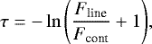
As OH absorption can occur at multiple velocities due to clouds along the line of sight, in total we find absorption in both main lines in 59 velocity components. Of these, we find 30 and 17 velocity components exclusively in the 1665 and 1667 MHz OH ground state transitions, respectively, and 12 in both lines, matching in velocity. We detect a higher number of OH 1665 MHz transitions, because the 1667 MHz transition was observed only around W43, during the pilot study, and during the second part of the THOR survey (see Sect. 2). Conversely, we sometimes find OH features in the 1667 MHz transition that have no counterparts in the 1665 MHz transition. This is expected, as the statistical weight of this transition is roughly twice as large, hence at a given sensitivity, optical depths and column densities twice as low can be probed. Examples of these are absorption at 7.0, 51.0, and 67.5 km s −1 towards G29.935−0.053 (Fig. 1).
The continuum sources with detections are listed in Table 1. The spectra of the detected absorption lines are displayed in Fig. D.1.
3.1.1 Sensitivity of the survey
The weakest continuum source with OH absorption has a continuum flux density of 0.1 Jy beam−1. As shown inFig. 3, stronger continuum sources are more sensitive to lower OH column densities. Therefore, the fraction of continuum sources that exhibit OH absorption is dependent on the continuum source strength (which sets the 4σ detection threshold, τmin): there are 291 continuum sources above a flux density of 0.1 Jy beam−1 at 20′′ ×20′′ (τmin ~ 0.5), of which 42 show OH absorption lines (14.4%). Above 1.0 Jy beam−1 (τmin ~ 0.04), 13 of 29 LOS have OH absorption lines (44.8%), while above 2.0 Jy beam−1 (τmin ~ 0.02), 3 out of 4 LOS (75.0%; this value should be taken with caution due to small number statistics). The cumulative detection fraction therefore is an increasing function of the continuum strength.
The reason for this increase is the dependence of the sensitivity of the optical depth (τ) on the strength of the continuum source:
 (1)
(1)
where Fline is the continuum subtracted OH absorption spectrum and Fcont the continuum emission. Contributions from OH emission to the observed signal are neglected, assuming the distribution of OH is smooth enough for emission to be filtered out by the interferometric observations and due to the small OH excitation temperatures in comparison to the continuum emission (see Sect. 3.2.1 for a more detailed discussion). While the OH transitions are mapped at rather uniform noise, the noise in OH optical depth, and therefore its sensitivity, is inversely proportional to continuum flux.
The OH ground state main lines show maser emission against many of the strong continuum sources. Non-detection of absorption lines is therefore not indicative of absence of OH in these lines of sight, but points to OH having different excitation conditions. Such regions typically have high dust temperatures and local densities (Tdust > 80 K,  cm−3; e.g., Guibert et al. 1978; Cesaroni & Walmsley 1991; Elitzur 1992; Csengeri et al. 2012, and references therein).
Artifacts also influence some of the spectra. This can be due to increased noise caused by residual radio frequency interference (RFI), which should be minor, as the data have been closely inspected for RFI prior to imaging. Also, strong line emission of non-thermal origin can leave various traces. At the position of a maser, adjacent channels are affected by Gibbs ringing, which is a recurring pattern in velocity of emission and absorption. If the maser emission is strong, channel maps around the peak velocity of the emission can be affected by increased noise levels and sidelobes. In the case of W51 Main (e.g., Ginsburg et al. 2012; G49.488−0.380 in this work), for example, it is difficult to discern negative sidelobes from true absorption. Absorption is present in this region as it is different from the shape of the interferometry pattern. Both, however, overlap and therefore a quantitative analysis of the affected velocity channels is not possible.
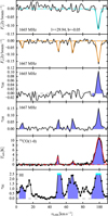 |
Fig. 1 Example spectra and optical depths at l = +29.935°, b = −0.053° (at 46″ resolution). Topmost two panels: 1665 and 1667 MHz absorption features. The fitted Gaussian profiles for the 1665 MHz line (cyan) and 1667 MHz line (orange) are overlaid. Two middle panels: optical depth of the 1665 and 1667 MHz transitions. Second panel from the bottom: emission of 13CO (1–0) in main-beam temperature (Tmb), overlaid with a fitted Gaussian profile (red). Lowermost panel: H I optical depth as measured from the absorption spectra. Lower limits (cyan dots) are given for saturated bins. The blue shaded area in the lower four panels denotes the area of the transitions, from which the column densities are determined. |
 |
Fig. 2 Detections of OH absorption at 1665 and 1667 MHz (red circles) overplotted on continuum emission at 1.4 GHz from the combined THOR and VGPS data (Beuther et al. 2016; Wang et al. 2018). |
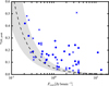 |
Fig. 3 Peak optical depth of the 1665-MHz transition (circles) and the 1667-MHz transition (crosses) vs. continuum flux density at 46′′. The sensitivity in OH optical depth is indicated by an average 4σ detection limit (black dashed curve). Variations in the detection limit among sightlines are indicated by the gray shaded area. |
3.1.2 H II region associations
In order to classify the continuum sources, we compare their location and the velocity of the detections to the emission from Radio Recombination Lines (RRLs) as reported in the WISE3 catalog of H II-regions (Anderson et al. 2014). The spatial selection criterium is overlap with the H II-regions using their angular sizes as reported in the WISE catalog. Since typical velocity differences between H II regions and associated molecular gas are lower than 10 km s −1 (Anderson et al. 2009, 2014), we use this as criterium for association in velocity.
For completeness, we also search the RRL observations in THOR (Beuther et al. 2016) and catalogs of dense molecular gas tracers associated with compact and ultracompact H II regions (e.g., NH3, HCO+; ATLASGAL survey; Urquhart et al. 2013, 2014; Contreras et al. 2013). While not adding new sources, counterparts of many OH detections could be found also in these datasets.
To confirm the presence H II-regions, we obtain information on the spatial extent and the spectral index of the continuum sources from the THOR continuum source catalog (Bihr et al. 2016; Wang et al. 2018). As H II regions would be located in our Galaxy, they are likely to be spatially resolved within THOR. The spectral index between 1 and 2 GHz helps to distinguish between thermal (with a spectral index of α ≳−0.1) and non-thermal emission sources (with a spectral index of α ~−1). Most of the continuum sources with RRL counterparts show thermal emission and are spatially resolved.
In total, 47 OH absorption components have its origin in molecular gas that is associated with H II regions in position and velocity, which represent 80% of all detections (see discussion in Sect. 4.1). We find that 38 out of 42 of the cm-continuum sources, against which the detections occur, show evidence of being H II regions. Three of the four other continuum sources are likely to be of extragalactic origin, as they are spatially unresolved and show non-thermal emission.
Twelve velocity components in the 1665 and 1667 MHz transitions, of which 4 are detected in both, originate from clouds that are not associated with H II regions. Neither RRL emission in the WISE catalog, nor dense molecular gas tracers are reported at the same vLSR. The peak opticaldepth is lower than seen for sources associated with H II regions. Accordingly, these absorption features are likely to originate from foreground, potentially diffuse clouds.
3.1.3 Distribution of sources in the Galactic plane
The distribution of OH absorption detections is strongly concentrated towards the Galactic midplane (Figs. 4 and 5), while relatively few detections are made at |b| > 0.5°. This follows the distribution of resolved Galactic continuum sources as a function of Galactic latitude (e.g., Bihr et al. 2016). Figure 4 is slightly skewed towards negative Galactic latitudes. This may be due to the sun being located above the true Galactic plane, while the sun is located at b = 0.0° in the Galactic coordinate system (Blaauw et al. 1960; Ragan et al. 2014). Depending on the distance of the object and the assumptions used to determine the physical location of the Galactic plane, sources which lie, e.g., in the Scutum–Centaurus Arm have Galactic latitudes of b = [−0.4°, −0.1°] (see discussion in, e.g., Goodman et al. 2014), which agrees well with the observed extent of the source distribution towards lower Galactic latitudes.
The histogram of sources vs. Galactic longitude (Fig. 5) reflects the Galactic structure, with a peak in the number of OH absorption sources at longitudes l = 30° and 50°, which are the tangential points of the Scutum and Sagitarius spiral arms, respectively (e.g., Reid et al. 2014). This confirms that most of the continuum background sources, against which OH absorption is seen, are of Galactic origin, as already indicated by the large number of H II regions in our sample.
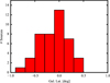 |
Fig. 4 Number of continuum sources with OH absorption detections vs. Galactic latitude. |
3.2 OH abundance
3.2.1 Line integrals
The OH column density is derived from the integrated optical depth in the main line transitions under the assumption that all molecules are in the four sublevels of the ground state arising from the Λ doubling and hyperfine structure (e.g., Elitzur 1992). The derived column densities are listed in Table 3.
Optical depths are computed from the line-to-continuum ratio. Contributions from large-scale emission are assumed to be filtered out by the interferometer. The emission term in the radiative transfer equation which includes the excitation temperature is therefore negligible (Tline = (Tex − Tcont)(1 − e−τ); where Tline and Tcont can be derived in Raleigh-Jeans approximation from the continuum-subtracted line flux and the continuum flux, Fline and Fcont). Even if this assumption did not hold true, at excitation temperatures of about Tex= 5−10 K, the approximation Tcont ≫ Tex underestimates the optical depth for a 5σ detection by less than ≪10% at 20′′ resolution and for sources with Fcont > 0.5 Jy beam−1 at 46′′ resolution. For weaker sources which show detectable extended continuum emission, the underestimation would be between 6 and 16% after smoothing to 46′′.
The integrated optical depth is determined by summation over all spectral bins of the absorption feature. The 13CO(1–0) emission is integrated over the same velocity range. If a corresponding 13CO(1–0) feature exists that is broader than the OH feature, the velocity range is chosen to enclose the 13CO(1–0) feature (see Fig. 1). For lines that have no 13CO(1–0) detection counterpart, 3σ upper limits are given for integrated emission and all derived quantities, under the assumption of an average line width of 4.0 km s −1 of the detected 13CO emission (Table 3).
Similarly, we derive the optical depth of H I from the line-to-continuum ratio, and give lower limits in the case of saturated absorption. A saturated channel is defined here as observed flux that is within 3σ of the zero level. This value is then used to calculate the lower limit (see cyan circles in the lowermost panel of Fig. 1). Analogously to the discussion above on τOH, emission in principle also affects the H I optical depth, but is likely to be filtered out here. For this reason, we do not attempt to correct for it, but note that the integrated optical depth here always represents a lower limit.
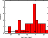 |
Fig. 5 Number of continuum sources with OH absorption detections vs. Galactic longitude. The 1665 MHz transition was observed over the entire region of the survey. The coverage of the 1667 MHz transition is indicated by the black bars. |
3.2.2 OHcolumn density
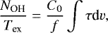
The OH column density is inferred for each main line separately, under the assumption that all OH molecules are in the ground state, 2Π3∕2(J = 3∕2). The OH column density is given by (e.g., Stanimirović et al. 2003)
 (2)
(2)
where NOH is the total OH column density in cm−2, Tex the excitation temperature in Kelvin, C0 = 4.0 × 1014 cm−2 K−1 km−1 s for the 1665 MHz transition and C0 = 2.24 × 1014 cm−2 K−1 km−1 s for the 1667 MHz transition (e.g., Goss 1968; Turner & Heiles 1971; Stanimirović et al. 2003, calculated using Einstein coefficients from Turner 1966). The filling factor f describes the solid angle fraction of the continuum source that is covered by the OH cloud. We assume that f = 1. The 1667 MHz transition is expected to be detected at higher signal-to-noise than the 1665 MHz transition because of its larger statistical weight, and therefore the 1667 MHz transition is used for further analysis whenever available. The calculated  ratios are given in Table 3.
The excitation temperatures of the OH transitions cannot be derived independently from their optical depth, as local thermal equilibrium between the levels of the two main lines is not necessarily given, and thus the excitation temperatures of both main lines may be different (e.g., Crutcher 1979; Dawson et al. 2014). A determination of both Tex and τ is in principle possible if additional emission observations were obtained at a position slightly offset from the continuum source. The OH emission is not detectable in the present dataset, as the OH emission is expected to be dominated by warm gas (e.g., Wannier et al. 1993) that varies on scales larger than the interferometric observations presented here. Hence, emission is filtered out. Observations of transitions to higher rotational levels of OH are not available for most sources and would require detailed modelling to constrain the excitation conditions of the hyperfine transitions in the ground state, which is beyond the scope of this paper. We therefore assume an excitation temperature from the literature in order to determine OH column densities (e.g., Stanimirović et al. 2003).
The excitation temperatures of the OH main lines have been found to differ relative to each other by 0.5–2.0 K (e.g., Goss 1968; Crutcher 1979; Dawson et al. 2014). This has also been seen in models (e.g., Guibert et al. 1978). The level populations may also be affected by radiative pumping (Csengeri et al. 2012; Wiesemeyer et al. 2016). Previous investigations reported excitation temperatures for the OH main line transitions between 3 and 10 K (e.g., Goss 1968; Turner 1973; Crutcher 1977; Colgan et al. 1989; Li & Goldsmith 2003; Bourke et al. 2001; Yusef-Zadeh et al. 2003). We therefore assume a uniform excitation temperature of Tex (1665) = 5 K for the 1665 MHz transition, which in principle can be higher by up to about a factor of two for OH gas associated with H II regions. We consider this in the systematic uncertainties (see Sect. 3.2.5). For transitions in which both main lines are detected, the medians of the column density distributions of each main line are offset. A better agreement between the samples is reached for a slightly higher excitation temperature for the 1667 MHz line of Tex (1667) = 6.7 K. We therefore adopt this value for the OH 1667 MHz transition in the following, while using Tex (1665) = 5 K in the OH 1665MHz transition.
Lines of sight with detections of OH 1665/1667 MHz absorption.
Line properties of OH 1665/1667 MHz absorption and 13CO(1–0) emission.
3.2.3 H2 column density
As proxy for H2, we use 13CO emission. Kinematically, 13CO is related to the OH gas. The line widths of the OH main lines and 13CO are compared in Fig. 6. The channel spacing of 1.5 km s−1 in the OH observations poses a limit of 2.5 km s−1 on the narrowest resolved line width for OH lines, while the full spectral resolution of 0.21 km s −1 is used for 13CO to disentangle different velocity components. Excluding the unresolved OH lines, the line widths of both tracers are found to be correlated4. In some cases, the 13CO emission features larger line widths than OH. One possible explanation is that larger parts of the molecular cloud contribute to the 13CO antenna temperature than to the OH absorption. For many continuum sources, only OH absorption from scales less than 46″ is recovered. As emission from within the entire beam contributes to the 13CO antenna temperature, the 13CO emission may average over larger parts of the cloud. Similarly, if the continuum source is located within the molecular cloud, 13CO emission contains information from all cloud depths (if not optically thick), while only parts of the cloud between the continuum source and the observer affect the OH absorption (see also Sect. 3.2.5). Depending on the velocity substructure of the cloud on scales smaller than the beam and along the line of sight, this can lead in both cases to larger line widths in the 13CO emission than in the OH absorption.
The column density of 13CO is determined from the integrated line profile (∫ Tmbdv) under the assumption that the gas is optically thin (e.g., Wilson et al. 2009, Eq. (15.37)):
 (3)
(3)
Average excitation temperatures of 13CO in molecularclouds are typically between 10 and 15 K, with values of up to 25 K in some cases (e.g., Frerking et al. 1982; Anderson et al. 2009; Pineda et al. 2010; Nishimura et al. 2015). We select an excitation temperature towards the upper end of this range of Tex= 20 K, as most of the OH detections are associated with H II regions. To account for possibly lower excitation temperatures, we assume an uncertainty of a factor of two on Tex, which results in an uncertainty of approximately a factor of two for  .
.
The column density of molecular gas is determined by assuming a constant 13CO abundance relative to molecular hydrogen molecules of 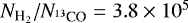 (Bolatto et al. 2013; Pineda et al. 2008). Uncertainties in this estimate due to optical thickness of 13CO or local variations inthe 13CO∕12CO ratio (Szűcs et al. 2016) are discussed in Sect. 3.2.5. If the 13CO(1–0) emission is not detected, we report upper limits for both
  and NH and lower limits on XOH.
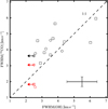 |
Fig. 6 Comparison of FWHM of OH and 13CO(1–0) lines. OH line widths of the 1665 MHz transition (squares) are used whenever the 1667 MHz transition (circles) was not available. Detections associated with H II regions are drawn in black, others in red. Arrows indicate spectrally unresolved lines. The dashed line indicates a 1:1 correlation. The bars in the lower right-hand corner of the figure indicate typical errors in both quantities. |
3.2.4 H I column density
To derive the H I column density, we assume a spin temperature (=Tex) of Tspin ~ 100 K (Bihr et al. 2015). The H I column density is given by (e.g., Wilson et al. 2009)
 (4)
(4)
Since the optical depth is a lower limit here (see Sect. 3.2.1), the H I column density is a lower limit as well. As Tspin may vary for individual regions by a factor of two, these limits are subject to a systematic uncertainty of the same factor.
In the following, we determine the OH abundance, XOH, both in terms of the column density of molecular hydrogen,  , and in terms of the total column density of hydrogen nuclei, which includes both atomic and molecular hydrogen, NH I and
  . NH is given by
  . The lower limits on NH i yield upper limits on XOH. The derived quantities from this section are listed in Table 3.
3.2.5 Systematic uncertainties
The systematic uncertainties of XOH,  and NH are estimated as follows. The
  ratio varies within molecular clouds and may be affected by global changes in the 13C isotope abundance with Galactocentric radius. First, the scatter of
  measurements has been found to be up to a factor of two within individual clouds (e.g., in Perseus; Pineda et al. 2008). We assume that this inflicts an uncertainty of a factor of two on
  . Second, the conversion used here has been determined in nearby Gould Belt clouds, but the 12C/13C isotope ratio increases with Galactocentric radius (Milam et al. 2005). With absorption sources located at Galactocentric radii between Rgc = 3 and 10 kpc, we assume that global variations in the 13C isotope abundance introduce an additional uncertainty of a factor of two on
  .
.
As described above, the assumptions regarding the excitation temperatures of OH, 13CO(1–0) and H I are likely to be valid within a factor of two as well. These result in a combined uncertainty of approximately a factor of 3.5 in  and NH, and a factor of four in XOH. As the H I absorption saturates in most cases, we can only determine lower limits to NH i.
Also, some of the 13CO(1–0) emission may be optically thick and give lower limits on  , and therefore upper limits on XOH. While
  as derived from 13CO may also be underestimated due to chemical effects (e.g., Szűcs et al. 2016), the derived H2 column densities have been compared with column densities derived from 870 μm dust emission (ATLASGAL), and we find reasonable agreement also towards high column densities within a factor of two.
At low CO column densities, molecular cloud regions may be traced that contain a significant fraction of “CO-dark” H2. This means that the column density of H2 would be underestimated and the OH abundance overestimated. The amount of “CO-dark” gas depends on the environment, i.e., on metallicity and the strength of the external radiation field. This makes a quantitative correction difficult, but the effect may influence detections for which H2 and H I column densities are comparable.
Geometrical uncertainties should also be considered. For the sake of simplicity, they are mentioned here only briefly, because they are difficult to quantify. First, the 13CO emission may trace molecular gas that is not accessible by the OH absorption observations. OH absorption occurs in material between theobserver and a continuum source, while material at any distance along the sightline contributes to the 13CO emission if optically thin. Most of the OH absorption detections are associated in velocity with the continuum source itself and by our definition separated from the continuum source by less than 10 km s−1. Assuming that the OH and 13CO gas, as well as the H II-region are part of the same molecular cloud, a fraction of the 13CO emission emerges from behind the continuum source as seen by the observer. This fraction depends on the structure of the molecular cloud and the relative position of the continuum source. For example, 50% of the 13CO emission will come from behind the H II region, if it is embedded in the middle of a spherically symmetric molecular cloud. No OH absorption can be measuredfor this part of the cloud, and the OH abundance will be underestimated. Velocity shifts between the different tracers in our data (<2 kms−1) indicate that at least some sources are affected by this. As we cannot constrain the structure of the cloud and quantify this effect, we choose not to correct for it here.
Second, crowded regions may contain multiple, overlapping H II-regions, which contribute to the observed continuum flux, if the continuum emission is optically thin. If OH absorption occurs along the line of sight in between such continuum sources, the observed continuum will overestimate the true continuum incident on the absorbing cloud. Therefore, the optical depth of OH would be underestimated. This is likely to affect lines of sight towards Galactic continuum sources that are located in crowded regions, such as the tangent points of spiral arms (G29, W43, and W51).
3.2.6 OH vs. H2 column density
OH and H2 column densities are shown in Fig. 7. NOH is derived from the 1667 MHz transition (circles) if available, and from the 1665 MHz transitions in the rest of the cases (squares). The absorption features are separated by color into regions that are associated (black) or not associated (red) with H II regions.
To investigate the correlation between NOH and  , we perform a linear regression in log-space,
  , to determine the slope m. The uncertainties are dominated by the systematic errors, i.e., possible variations of NOH and
  by a factor of 2 and 3.5, respectively (see Sect. 3.2.5). To properly take into account their impact on the correlation, we estimate the distribution of slopes m given these uncertainties and the stochastic measurement errors. We do not include upper limits. We sample the posterior distribution of m by performing linear regressions on multiple, artificial representations of the data, which are inferred from the uncertainty distributions of the measurements.
We create a large number of artificial datasets (ndatasets = 105). Each artificial dataset has the same number of points as our measured sample, but instead of containing the measurements itself, each point is replaced by randomly drawing an artificial datapoint from the uncertainty distribution. We also “bootstrap” each of these simulated datasets, i.e., randomnly assigning weights to the points to reduce the importance of each individual measurement. From the linear regression on each of these artificial datasets, we obtain a distribution of slopes with median and 16%-, 84%-percentiles of  (see also Fig. B.1). The green line in Fig. 7 shows the median slope.
We interpret this result as an indication of a weak, sublinear correlation between NOH and  . A direct proportionality between the two parameters is unlikely, given the distribution of slopes. The sublinear relation between NOH and
  yields a decreasing OH abundance (
 ), as discussed in the following sections. The analysis shows that a correlation is present in the data, but for tighter constraints, follow-up studies are needed to provide more data and/or to decrease the systematic uncertainties.
3.2.7 OHabundance at different hydrogen column densities
Figure 8 shows the OH abundance in terms of the molecular hydrogen column density ( ) vs.
) vs.  . The literature value for
  is plotted asa dashed gray line, and the right axis shows the data in terms of this value (e.g., Guelin 1985; Langer & Graedel 1989; van Langevelde et al. 1995; Liszt & Lucas 1999, 2002). The OH abundance is found to be anti-correlated with
  over the range of probed cloud depths (
 ). Above
  (AV ~ 20 mag)5, most of the abundances are lower than the literature value, while the abundances at lower H2 column densities are slightly higher.
We use the H I absorption data as lower limit for the column density of atomic hydrogen, and show the OH abundance with respect to the total number of hydrogen nuclei in Fig. 9. While the overall trend is similar to that seen in Fig. 8, the atomic hydrogen content probed along the line-of-sight is comparable to molecular hydrogen for a few detected components with low molecular hydrogen column densities (e.g., for G29.935−0.053 at 7.0 km s−1 and G29.957−0.018 at 8.0 km s−1).
We see aclear anti-correlation between XOH and  for OH associated with H II regions (black). Measurements which are not associated (red), follow this trend in Fig. 8. In the abundance with respect to all hydrogen nuclei (NOH∕NH) in Fig. 9, this trend appears not to be present in the red data points, since the lowest data points have significant contribution from atomic hydrogen. As the H I column densities are lower limits, the abundances are upper limits, favoring an even shallower trend of XOH in this NH column density regime. As mentioned in Sect. 3.2.5, also the fraction of “CO-dark” H2 may be significant for most of the detections which are not associated with H II regions and the lowest of the measurements associated with H II regions, which would place them at higher
  (and NH) and lower XOH in Figs. 8 and 9.
The red data points fall into similar ranges of visual extinction as probed by many earlier studies. The OH abundance for visual extinctions of AV < 7 mag has been reported in the literature to be constant at XOH = NOH∕NH = 4 × 10⁻⁸ (e.g., Goss 1968; Crutcher 1979). The median OH abundance for this group of points here is 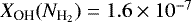 with a scatter of ΔXOH = 0.27 dex and XOH(NH) = 6.0 × 10⁻⁸ and a scatter of ΔXOH = 0.22 dex.
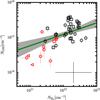 |
Fig. 7 Comparison of the OH column density from the 1665 MHz (squares) and 1667 MHz transitions (circles) to that of H2 as inferred from 13CO(1–0) emission. Column densities from absorption features overlapping in velocity with H II regions (black) and with no such counterpart (red) divide the plot into regions with higher and lower hydrogen column densities. Triangles denote upper limits on |


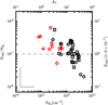 |
Fig. 8 OH abundance |


3.3 Satellite line transitions
Satellite lines of the OH ground state transitions are rarely found in local thermodynamic equilibrium with the main line transitions. While the main lines are seen in absorption, the satellite lines can be anomalously excited and may show conjugate emission and absorption, often at equal strength (e.g., towards G18.303−0.390 and G25.396+0.033; see Fig. C.1). Table 4 catalogs conjugate satellite transitions found in this survey. The qualitative satellite line behavior reflects the physical conditions of the gas, such that we can use this to estimate OH column densities for a subsample of sources.
Emission in the 1612 MHz transition with absorption in the 1720 MHz transition is found in 14 instances. Emission in the 1720 MHz transition with absorption in the 1612 MHz transition occurs in three cases (e.g., towards G32.798+0.190 at 90 km s −1; see Table 4).
Satellite line reversal, i.e., the transition from absorption to emission (or vice versa) across the line, is seen along 3 lines of sight. Both satellites mirror each other: at lower velocities, the 1720 MHz line is in emission, while the 1612 MHz line is in absorption. At a certain velocity, the behavior reverses. This is found in the following cases in this work: G19.075−0.288 at 67.5 km s −1, G32.798+0.190 at 14.0 km s−1, G49.369−0.302 at 63.5 km s−1. Lines of sight, for which the full reversal profile is not detected in both satellite lines, but which are indicative of this behavior, are: G29.935−0.053 at 98.5 km s −1, for which reversal in the 1612 MHz transition is detected, but the 1720 MHz line is seen only in absorption at higher velocities, and not detected in emission at lower velocities. Towards G37.764−0.215 at 65.0 km s−1, G49.206−0.342 at 63.5 km s−1 and G49.369−0.302 at 49.5 km s−1, 1612 MHz absorption is seen at low velocities without conjugate emission in the 1720 MHz transition, while at higher velocities, the 1720 MHz transition is in absorption without conjugate emission in the 1612 MHz transition.
In the other cases, the satellite lines are not detected or only one transition of the two is detected. Indication of absorption in both lines can be seen in G61.475+0.092 at +21.2 km s−1, with the satellite line strengths differing from each other, as is expected since the lines are typically not in local thermal equilibrium.
The conjugate emission and absorption of the satellite lines has been noted in previous studies (e.g., Goss 1968; Crutcher 1977; van Langevelde et al. 1995; Brooks & Whiteoak 2001; Dawson et al. 2014), and is the result of overpopulation of either theF = 1 or the F = 2 hyperfine energy levels of the ground state and mutual depletion of the others (e.g., Elitzur 1992, Sect. 9.1). As the satellite lines are transitions with |ΔF| = 1, they are affected by the relative population changes, while the main line transitions with |Δ F| = 0 may not be affected by this particular inversion mechanism.
There are different pumping mechanisms that may be responsible for the population inversion (see discussion in, e.g., Frayer et al. 1998). In all cases, transitions from higher rotational levels to the ground state need to become optically thick (e.g., Elitzur 1992; van Langevelde et al. 1995): if the infrared transitions from either the 2Π3∕2(J = 5∕2) or the 2Π1∕2(J = 1∕2) states into the ground state become optically thick, the 1720 MHz or the 1612 MHz transition, respectively, is seen in inversion. If both transitions are optically thick, inversion of the 1612 MHz transition is seen. As the transitions from the 2Π3∕2(J = 5∕2) excited state become optically thick at lower NOH than from the 2Π1∕2(J = 1∕2) state, there exists a typical OH column density at which the transition from 1720 to 1612 MHz inversion takes place. This has been used and modeled by van Langevelde et al. (1995) for a molecular cloud heated by a background H II region and satellite line reversal was found to take place at ≈ 1 × 1015 cm−2 km−1 s.
Assuming this geometry also for the sources in this sample, this model provides a possibility to estimate NOH. The column density depends on the velocity dispersion of the gas (NOH ≈Δv × 1 × 1015 cm−2 km−1 s). As we have no direct measure of the line width at the velocity of the reversal of the inversion we use as approximation the full width of half maximum of the 1665 MHz main. The transition occurs at NOH ≈ 7.4 × 1015 cm−2 for G19.075−0.288, at NOH ≈ 1.2 × 1016 cm−2 for G32.798+0.190 and at NOH ≈ 4.4 × 1015 cm−2 for G49.369−0.302.
We compare the estimates for G32.798+0.190 and G49.369−0.302 to NOH derived from the main lines in Sect. 3.2. G19.075−0.288 is omitted here, as the reversal velocity does not match the velocity of the maximum optical depth of the 1665 MHz transition (Fig. C.1). For G32.798+0.190 and G49.369−0.302, NOH determined from the main lines is a factor of 3–4 lower than the estimate from the satellite lines. The line width used for the NOH estimate from the satellite lines could be an overestimate if multiple components are blended into the feature. Alternatively, the discrepancy could be an indication of higher main line excitation temperatures than the assumed Tex (1665) = 5 K. To match the estimates from the satellite lines, excitation temperatures of Tex ≈ 15−20 K would be required.
A similar discrepancy has been noted in Xu et al. (2016), who find lower OH column densities than needed to reproduce the observed emission in the 1612 MHz transition. They attribute this to other excitation mechanisms, such as collisional excitation in shocks (e.g., Pihlström et al. 2008), which are also not taken into account in the model by van Langevelde et al. (1995).
Recently, employing non-LTE modeling of all four 18 cm OH emission lines, Ebisawa et al. (2015) have used the relative intensities of main-line and 1720 MHz emission and 1612 MHz absorption in the Heiles Cloud 2 and ρ Oph to derive kinetic temperatures that are significantly higher in translucent than in dark molecular regions. This indicates that OH appears to be able to probe the interface between molecular and warmer atomic material. Such an analysis is beyond the scope of the present paper, but can be included in a future study.
Derived quantities from OH 1665/1667 MHz and H I absorption and 13CO(1–0) emission.
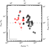 |
Fig. 9 OH abundance XOH = NOH∕NH vs. NH. The total column density of hydrogen nuclei, NH, is inferred from 13CO(1–0) emission and H I absorption. As the H I column density represents lower limits, the OH abundances represent upper limits. Colors and symbols are as in Fig. 8. The right axis shows the OH abundance in units of the typical OH abundance in diffuse clouds of 4 × 10⁻⁸ (Crutcher 1979, indicated also by the dashed gray line). |
Conjugate inversion and anti-inversion of satellite lines.
3.4 Extended OH absorption: the example of W43
Spatially resolved OH absorption is seen against a subsample of the continuum sources (examples of these are the Galactic H II regions M17, G18.148−0.283, G37.764−0.215, G45.454+0.060 and G61.475+0.092). This allows for a comparison of column density and kinematic structure in different physical regimes: the ionized gas phase is traced by continuum emission and RRLs, the cold neutral medium is traced by H I absorption and the molecular gas regime is traced by different CO isotopologues and far-IR continuum emission. We present the star-forming region W43, as an example of what can be learned from this data.
W43 is one of the largest molecular cloud complexes in our Galaxy. It is located at the intersection of the Scutum–Centaurus spiral arm with the Galactic bar, is actively forming stars at a high rate and is dynamically complex (e.g., Nguyen Luong et al. 2011; Motte et al. 2014; Bihr et al. 2015). It is composed of multiple sub-regions, most prominently the W43-main and W43-south regions, which themselves break down into smaller regions of molecular gas (e.g., Carlhoff et al. 2013). In W43-main, complex structure is also indicated by the high H I column densities (e.g., Liszt 1995; Motte et al. 2014; Bihr et al. 2015), which suggests the presence of several molecular clouds along the line-of-sight (Bialy et al. 2017).
Different evolutionary stages of stars and clouds coexist and appear to be influencing each other: an OB cluster at the center of W43-main, which contains Wolf–Rayet stars, includes a strong source of ultraviolet photons (e.g., Smith et al. 1978; Blum et al. 1999); these provide the ionization and heating of the central H II region (e.g., Reifenstein et al. 1970; Lester et al. 1985). There is evidence for a second generation of star formation, indicated by clumps of dense gas and ultra-compact H II regions (e.g., Motte et al. 2003; Bally et al. 2010; Beuther et al. 2012), which conveys the picture of gas compression driven by the central H II regions (e.g., Blum et al. 1999; Balser et al. 2001). In the environment of W43-main, pre-stellar cores manifest higher gas temperatures than in quiescent regions due to the heating by the central cluster, possibly affecting the number of stars formed in the future (Beuther et al. 2012). Adding to the complexity of the region, observations of molecular and ionized gas tracers revealed several velocity gradients and substructures of different morphologies (e.g., Liszt 1995; Balser et al. 2001; Carlhoff et al. 2013). The gas streams on global scales in molecular and atomic gas indicate that the H to H2 conversion is ongoing (Motte et al. 2014). Dynamical interaction between clouds has been investigated on smaller scales with SiO emission, which possibly emerges from low velocity shocks in mm-emission peaks (e.g., Nguyen Luong et al. 2013; Louvet et al. 2016).
The extended OH absorption in W43 is displayed in the left panel of Fig. 10, in which the optical depth has been integrated between 78.0 and 100.5 km s−1, and all maps are shown at an angular resolution of 20′′ ×20′′, corresponding to a spatial scale of 0.5 pc at a distance of 5.5 kpc (Zhang et al. 2014). Intrinsically, absorption is seen towards strong continuum emission peaks, as the sensitivity to find absorption increases with continuum emission strength. However, the strongest integrated optical depth peaks do not coincide with continuum emission peaks, but are seen towards the mm dust emission sources MM1 and MM36 (nomenclature taken from Motte et al. 2003). The integrated OH absorption varies by a factor of 3 around the central H II region, and is higher by an order of magnitude towards the outer parts of the T-shaped continuum emission: at MM3 and towards MM1, the total line-of-sight column density is approximately 7 × 10¹⁵ and 9 × 1015 cm−2, respectively, while the column density is between 0.5 and 2 × 1015 cm−2 around the central H II region, assuming an excitation temperature of Tex = 5 K in both cases.
Figure 10 compares the optical depth of the OH 1667 MHz transition to ATLASGAL 870 μm dust emission (Schuller et al. 2009) and to C18O(2–1) emission (Carlhoff et al. 2013). The middle panel displays the ratio of integrated OH optical depth to 870 μm dust emission, while the right panel displays the ratio to integrated C18 O(2–1) emission. Both the OH and C18O(2–1) data have been integrated between 78.0 and 100.5 km s−1. For the OH optical depth only such pixels contribute to the integral that are significantly detected in the absorption data. The value of the ratio maps are shown for relative comparison of different parts of the region, motivated by the hypothesis that all the tracers are optically thin and hence contribute linearly to the column density of the species (the optical thickness of the tracers is discussed further in Sect. 4.4). Thus, the ratios quoted here represent no physical quantity directly but their variation across the map can be indicative either of OH abundance or excitation variations.
The integrated C18O and 870 μm emission are shown as contours in Fig. 10. There are enhancements towards the central continuum source, towards MM1 and MM3 in both tracers. The strongest peak in the C18O emission is towards the central part of the T-bar, and is slightly offset from the peak of the continuum emission. The ATLASGAL emission peaks more strongly towards MM1 and MM3. At MM1, continuum emission and C18 O emission are slightly shifted awayfrom the 870 μm emission.
Within the central part of the T-bar, the ratio of OH optical depth to C18 O emission is around 0.05, and slightly higher on the left side of the central continuum peak. This is similar in the 870 μm emission, where the ratio is between 0.2 and 0.3, and by a factor of 2 higher on the side facing MM1. The ratio is around a factor of 4–9 higher against the MM1 and MM3 sources in both tracers. This increase is slightly higher for the ratio to C18 O emission than to 870 μm emission, which is consistent with the stronger increase of the 870 μm emission towards these sources. Against “Pos. 1”, however, the ratio to ATLASGAL 870 μm emission is by a factor of ~5 higher than in the central continuum emission region. The increase in this ratio is also seen in the C18 O emission.
In order to understand this comparison better, Fig. 11 shows the ratio of OH optical depth and C18 O in velocity ranges of 4.5 km s −1 (after binning three channels of 1.5 km s−1). Between 81.0 and 84.0 km s −1, OH absorption is seen against the central H II region and “Pos. 1”. C18O is significantly detected only in few locations, and we include upper limits in the plot (encircled by blue contours). Ratios are found between 0.3 and 0.4. A similar ratio is seen between 90 and 93.0 km s −1 towards MM3, MM1 and “Pos. 1”. In this velocity range, however, the OH ratio at the center of the T-bar is rather low, between 0.03 and 0.1. The ratio increases for MM1 towards 0.5 between 94.5 and 97.5 km s −1.
To conclude, variations in OH to C18O ratio are seen also when refining the integration interval. There seem to be two regimes – the central part of the H II region exhibits a ratio of ~ 0.05, while for other locations and other velocities, we find a ratio of ~0.3. At lower velocities, also the central part of the H II region is seen at ratios of ~ 0.3. This is further discussed in Sect. 4.4.
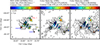 |
Fig. 10 Comparison of τ(OH 1667 MHz), dust continuum emission at λ = 870 μm, and C18 O(2–1) emission in the W43 star-forming region. In the left panel, the integrated optical depth of the OH 1667 MHz transition between 78.0and 100.5 km s−1 is displayed in colors. For each pixel, only channels that are detected at a 3σ level contribute to the integrated τ-map. It is overlayed with contours of the 18 cm continuum emission (black, at levels of 0.1, 0.2, 0.4, 0.6, 0.8, 1.0, 1.25, 1.5 and 1.75 Jy beam−1). Middle panel: ratio of the integrated τ(OH) map to 870 μm ATLASGAL emission (Schuller et al. 2009), which traces dense gas (the dust emission is overlayed in black contours, at levels of 0.5, 1.0, 2.0, 3.0, 4.0, 5.0, 7.0 and 10.0 Jy beam−1). Right panel: ratio of τ(OH) to C18 O(2–1) emission (Carlhoff et al. 2013), integrated over the same velocity range (the velocity integrated C18 O(2–1) emission is overplotted in black contours at levels of 6, 9, 13, 15, 17, 19, 23 K km s −1). All data have been smoothed to a common resolution of 20′′, corresponding to spatial scales of 0.5 pc. In the left panel, the central Wolf–Rayet/OB cluster is marked by a black star, while the dense clumps MM1 and MM3 (Motte et al. 2003) are marked by blue stars. The upper end of the T-bar-shaped continuum emission is marked as Pos. 1 for easier reference in the text. For readability, the values of the ratio are displayed for selected positions in the figure. |
4 Discussion
4.1 Distribution of OH in the Galactic plane
Recent single-dish observations of the OH ground state transitions find OH to be extended over wide areas in the Galactic plane (Dawson et al. 2014). The number of absorption detections found in this work is at first glance small relative to the number of cm-continuum sources available in the Galactic plane (e.g., Bihr et al. 2016) and needs to be discussed in terms of the varying sensitivity limit with continuum source strength.
We detect OH absorption mostly against extended Galactic cm-continuum background sources that show a spectral index in agreement with that of free-free emission from H II regions. The lower number of detections of OH in diffuse clouds not associated with H II regions is likely due to the sensitivity limits indicated in Fig. 3. While we do detect OH absorption at a variety of optical depths below τ ≤ 0.2 at continuum flux density >1 Jy beam−1, at lower continuum surface brightness the sensitivity is not high enough to detect sources with τ ≤ 0.05−0.1. As the majority of the continuum sources havea flux density <1 Jy beam−1, we pick up largely absorption at higher optical depths. The increase of the relative number of detections with strength of the continuum source is a further indication that some of the diffuse OH gas (e.g., Dawson et al. 2014) remains undetected for this group of sources.
As diffuse clouds are typically found to have low optical depths (e.g., Liszt & Lucas 1996), we are therefore biased towards higher column densities. As comparison, according to Dickey et al. (1981) using the Nançay telescope at 3.′5 resolution, OH optical depths in diffuse clouds have been found to be approximately 0.05 in a 1 km s −1 channel in the 1667 MHz transition. Higher optical depths were found by, e.g., Goss (1968), Yusef-Zadeh et al. (2003) or Stanimirović et al. (2003). OH gas was associated with the Galactic continuum sources, H II regions or supernova remnants (SNR). The detections presented here match more with the latter categories.
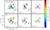 |
Fig. 11 Ratio of integrated τ(OH 1667 MHz) absorption and C18O(2–1) emission in W43. The top-left panel is the same as the rightmost panel in Fig. 10 and is shown for orientation. The other panels show the ratio of τ(OH 1667 MHz) and C18 O(2–1) at the indicated velocities after binning three channels of 1.5 km s−1 width. Overlayed on all panels are contours of 18 cm continuum emission (black, in levels of 0.1, 0.2, 0.4, 0.6, 0.8, 1.0, 1.25, 1.5 and 1.75 Jy beam−1). The 1667 MHz optical depth has been masked at 3σ detection levels in the original OH absorption data. For pixels with no C18O emission counterpart, 3σ detection limits have been used, and are indicated by blue contours. The ratio is quoted in brackets for these locations. |
4.2 OH as tracer of hydrogen gas
In Sect. 3.2, we compared the OH abundance to the column densities of molecular hydrogen and hydrogen nuclei (hydrogen atoms and molecules). These comparisons are shown in Figs. 8 and 9. OH abundance is found to be decreasing with increasing hydrogen column density. The OH column density is not directly proportional to molecular column density. Therefore, the OH columns densities span a smaller dynamic range than molecular hydrogen. This also indicates that OH traces only specific ranges of molecular cloud column densities.
At any given hydrogen column density, the OH abundance shows variations of a factor of two, which is within the systematic uncertainties. The median value of the OH abundance with respect to  is 1.3 × 10⁻⁷. Within the systematic uncertainties of a factor of 4, this is in agreement with the values reported in the literature, NOH/
 (e.g., Liszt & Lucas 2002).
A constant OH abundance with respect to NH, as reported by, e.g., Crutcher (1979), can be reproduced – albeit with large scatter – for OH absorption with visual extinctions below AV ≈ 10-20. A median abundance of XOH(NH) ≈ 6.1 × 10⁻⁸ is found for AV < 20. We include atomic hydrogen, as OH may be present in transition regions that contain significant amounts of atomic hydrogen (e.g., Xu et al. 2016; Tang et al. 2017). The H I column density affects the OH abundances at the lowest molecular hydrogen column densities probed, when both are of similar strength. XOH may even be lower in this regime, since the NH I measurements are lower limits and the  column densities may be underestimated, if the “CO-dark” gas fraction is significant (see Sect. 3.2.5).
Crutcher (1979) finds an abundance of XOH = 4.0 × 10⁻⁸, in a range of visual extinction of AV = 0.4−7 (see also review by Heiles et al. 1993), which is within the errors of our results. These results are based on studies of nearby molecular clouds (Perseus, Ophiuchus and Taurus), the SNR W44 and line-of-sight observations against extragalactic continuum sources, therefore mainly including observations towards diffuse molecular/translucent clouds (e.g., Snow & McCall 2006) that probably have environments similar to those of clouds that are not associated with H II regions in the sample presented here.
Above visual extinctions of AV ≈ 10−20, some OH abundances are found to be lower than the literature abundance, which is in agreement with theoretical predictions (e.g., Heiles et al. 1993). Oxygen to form OH at these extinctions is likely to be removed from the gas phase by the formation of CO and through the formation of water and its subsequent freeze-out onto grains. Far ultraviolet (FUV) radiation may counteract this removal: models of photon dominated regions (PDRs) indicate that the local abundance of OH peaks between cloud depths of AV ≈ 3−7 (e.g., Hollenbach et al. 2009, 2012). According to Hollenbach et al. (2009), the abundance of water in these regions depends on the photodesorption of water ice from dust grains, and OH forms by photodissociation of water in the gas phase. Both water and hydroxyl gas phase abundances thus depend on the flux of the far ultraviolet (FUV) radiation, and decrease once the FUV radiation is efficiently attenuated deeper inside the cloud. As NOH in this work represents a line-of-sight averaged density, OH from more embedded regions in the molecular cloud may contribute less to NOH than 13CO does to  , which may yield a decrease in the line-of-sight averaged OH abundance.
Anotherpossibility for the low OH abundances at high visual extinctions is that the OH excitation temperatures could be higher, approaching the kinetic temperatures in denser and warmer regions of the star forming molecular clouds in our sample. An excitation temperature of, e.g., 20 K would place most of the lowest measured OH abundances at XOH ~ 1 × 10⁻⁷ in Fig. 8. As many OH abundances at lower  lie above this value, the trend in Fig. 8 is likely to persist but to be less steep if higher excitation temperatures at higher
  were assumed. This effect is difficult to assess from our data alone, as the excitation temperature cannot be determined independently of the optical depth. Hence, more detailed modelling or targeted observations would be necessary to resolve this ambiguity.
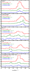 |
Fig. 12 Spectra of τOH in the 1665 and 1667 MHz lines, as well as of emission in C18O(2–1) line. The spectra are extracted towards positions MM1, MM36, WR and “Pos. 1” as indicated in Figs. 10 and 11, as well as towards the central part of the T-bar. Towards MM3, the channel at 96 km s −1 of the OH 1667MHz absorption is masked because of sidelobes of close-by maser emission. |
4.3 Comparison with OH column density measurements from other transitions
In this section, we briefly discuss results on the OH column density that had been inferred from observations of other OH transitions. Section 3.3 described the morphologies of the satellite line transitions inside the OH ground state. In three regions, reversal of the 1612 MHz transition from absorption to emission and of the 1720 MHz transition from emission to absorption has been seen. As discussed in Sect. 3.3, the column density at the transition velocity was inferred using modeling results from van Langevelde et al. (1995). The column densities appear to be by a factor of 3–4 higher than the value inferred from the main lines. As an excitation temperature of 5 K was assumed for the OH ground state transitions, this discrepancy could be remedied by assuming an excitation temperature of 15–20 K, where values up to ~15 K have been found also in previous works (Colgan et al. 1989).
Additionally, rotational transitions in the far infrared wavelength regime (e.g., Wiesemeyer et al. 2012; Csengeri et al. 2012) or electronic transitions in the optical regime (e.g., Weselak et al. 2010) can be used to study the OH column density. The crossmatch with our sample yields a match only for G49.488−0.380 with the source W51e2 in Wiesemeyer et al. (2016). However, the column density at velocities at which OH is detected in this work, is not reported, as the 2Π3∕2 J = 5∕2 ← 3∕2 transitions at 2.5 THz saturate between 50 and 80 km s−1.
The OH abundances determined here agree within our systematic uncertainty with the abundances inferred from optical and infrared transitions (Weselak et al. 2010; Wiesemeyer et al. 2016). Figure 13 compares the OH abundances determined here with OH abundances derived from the THz transitions at different lines of sight by Wiesemeyer et al. (2016). Within the sensitivity limits of our survey, for abundances using HF as tracer of H2, good agreement is seen between both datasets. This is also true for abundances using CH as tracer of H2, although some points are present between  ≈ 6 and 10 × 1021 cm−2, which show lower abundance, but are still within uncertainties. Also, for low H2 column densities, our measurements appear to be sensitivity limited (some measurements from Wiesemeyer et al. (2016) fall below the sensitivity limits indicated in Fig. 13). This comparison affirms the conclusion from Sect. 4.1 that the sample of OH absorption presented here indeed is biased towards high NOH. Conversely, some continuum sources are strong enough to reveal OH absorption in more diffuse molecular cloud regions. Albeit the large systematic uncertainties of XOH here, Fig. 13 shows that the variations in OH abundance at any given
  persist when using alternative methods to measure NOH and
  , which are possibly less prone to systematics.
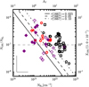 |
Fig. 13 Comparison of the OH molecular abundances from this work to abundances measured in Wiesemeyer et al. (2016). Data, symbols and systematic uncertainties as in Fig. 8. Measurements from Table 4 of Wiesemeyer et al. (2016) are overplotted as purple diamonds. Filled diamonds use HF as proxy for the H2 column density. Empty diamonds use CH. If both HF and CH measurements are available, OH measurements are drawn twice. Black diagonal lines indicate sensitivity limits of XOH for typical 4σ limits on optical depth in the OH main lines and assuming a line width of 2.5 km s −1 (the detection limits of τ = 0.025, 0.05 and 0.1 are acchieved for continuum sources stronger than Fcont = 2.10, 1.05 and 0.53 Jy beam−1, respectively). |
4.4 Extended OH absorption towards W43
As W43 is structured in a complicated way, and OH chemistry and excitation may vary strongly in different environments, there may be multiple explanations for variations in the ratios of OH optical depth to C18 O and 870 μm emission. For example, there are temperature gradients present in the entire region, which may affect the dust emission.
The peak optical depth of the 1667 MHz transition is typically at τ < 1 in W43. Exceptions are MM1 and MM3, for which optical depth peaks of τ1667 ~ 1.2 indicate that the line becomes optically thick (Fig. 12). For MM1, the 1665 MHz transition peaks at τ1665 ~ 0.6. Therefore, the ratio of the main lines (τ1667∕τ1665 ≈ 2.0) is within errors of the expected ratio for LTE excitation of 1.8. For MM3, the ratio of the main lines is closer to unity with τ1665 ~ 1.0, indicating that the transitions are not in LTE. As we have no probe of the excitation temperatures, this cannot be further assessed here. We note, however, that deviations from LTE in the OH hyperfine ground state transitions appear to be a common phenomenon (e.g., Li et al. 2018).
In order to minimize the chance of the CO tracers to become optically thick, we choose data from the C18 O(2–1) transition. Optical thickness even of this transition cannot be ruled out in the entire region, and it will trace regions at higher densities than the 13CO(1–0) used in the rest of the analysis. However, in order to investigate variations on a 20′′ scale (0.5 pc) in W43, these data provide information about the molecular gas at matching spatial resolution. As the datasets presented here cannot constrain whether these variations are due to abundance variations or differences in the excitation behavior, we limit the discussion to a qualitative description of the results.
In Fig. 11, the enhancement in the OH to C18 O ratio around 82.5 km s −1 coincides with a peak in radio recombination lines (see velocity distribution of H92α in Fig. 6 of Balser et al. 2001 or of cm-RRLs from THOR in Fig. 2 of Nguyen-Luong et al. 2017). At this velocity, possibly a photon-dominated, partly ionized region of the cloud is seen, in which models of photon-dominated regions predict the peak of the OH abundance (e.g., Hollenbach et al. 2012).
The OH 1667 MHz to C18O ratios in the center of W43-main at 90–93 km s−1 are found to be lower (≤0.1; Fig. 11, bottom left panel). This may be due to different physical or chemical conditions of the OH gas, which are difficult to disentangle in a crowded region like W43. Alternatively, this can be a consequence of systematically underestimating the OH optical depth. As described in Sect. 3.2.5, the measured continuum is higher than the true continuum incident on the OH gas, if H II-regions contribute to the continuum emission, which lie between the absorbing cloud and the observer.
This geometry is likely to be present here. The continuum emission at the Wolf–Rayet/OB cluster originates from the H II-region, which emits RRLs between 80 and 90 km s −1. At the T-bar, the RRLs peak between 90 and 100 km s−1, or even at higher velocities close to MM1. Since H II-regions are expanding, gas at lower velocities may be located closer to the observer than higher velocities gas. Absorbing OH gas at 90−100 km s−1 would therefore lie between two H II-regions and its measured optical depth can be lower than the true value.
The distribution of absorption in OH and emission in C18 O is in agreement with this scenario. In Fig. 12, we show spectra of both molecules at different positions. Towards the central Wolf–Rayet cluster, only absorption at 82 km s −1 is present, while not detected between 90 and 95 km s−1 in spite of the presence of C18O emission. Towards the center of the T-bar, absorption becomes visible in both velocity ranges. How much and at which lines of sight the optical depth is influenced by this effect, depends on the fractional contribution of each H II-region to the continuum emission. A quantitative assessment of this is beyond the scope of this work.
Close to MM1, the peak of the OH absorption occurs between 96 and 97.5 km s −1. The average velocity of the MM1 complex has been found to be at 98 km s −1 (Nguyen Luong et al. 2013) and more resolved observation in HCN(1–0) and SiO(2–1) emission show peaks between 97 and 94 km s −1, respectively, when going from MM1 towards the center of W43-main (Louvet et al. 2016). Louvet et al. indicate low velocity shocks in this region. While this needs to be confirmed, such shocks may produce temperatures that can enhance the OH abundance by activating neutral-neutral chemistry (Neufeld et al. 2002). However, the presence of additional, enhanced UV radiation may be required to produce OH, as neutral-neutral chemistry at high temperatures typically leads to water production (e.g., van Dishoeck et al. 2013). Near MM3 we see emission over a large range of velocities, with a clear peak in optical depth at 93 km s −1 in the 1665 MHz line, in agreement with N2 H+ and SiO peaks at the same velocity (Nguyen Luong et al. 2013).
5 Conclusions
This work gives an overview on the OH absorption against strong continuum background sources as inferred from the THOR survey. This is the first survey-style analysis with the VLA over a significant fraction of the inner Milky Way in the range between l = 15° and l = 67°. We detect 59 distinct absorption features against 42 continuum background sources. Most of the absorption is found against Galactic H II regions.We discuss the detection limit in terms of the continuum source strengths.
Using 13CO(1–0) as tracer for
 , we compare the OH abundance (
 ) at different
  . The OH abundance decreases with increasing hydrogen column density, especially for OH detections in molecular clouds that are associated with H II regions. This can be due to probing cloud regions where the OH in the gas phase is significantly depleted, although varying excitation conditions may provide an alternative explanation. The median abundance is found at
 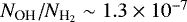 , in agreement within errors with previous studies.
-
At low column densities, the atomic hydrogen fraction of the gas along the line-of-sight becomes comparable to molecular hydrogen. The OH abundance (NOH∕NH) is found to decrease with increasing total hydrogen nucleus column density for Av > 20, but for lower extinction lines of sight, the data are consistent with a constant abundance having median value NOH∕NH ~ 6.1 × 10⁻⁸.
-
Extended OH absorption is seen against W43. The OH absorption is compared to ancillary data of 870 μm and C18O emission. At an angular resolution of 20′′ ×20′′, we find variation in the ratios of OH optical depth to emission in 870 μm and C18O, especially towards mm emission sources in the region.
Studies of OH provide a unique insight into the physical conditions of the ISM, particularly the transition between diffuse gas and molecular clouds. This first unbiased interferometric survey is a contribution to the characterization of the variation of OH absorption properties throughout the Galaxy. This work may provide a starting point for theoretical and observational follow-up studies with deeper observations at higher velocity resolution, to expand the sample towards fainter sources with narrower line widths, and in combination with other observational data to resolve the physical conditions of the OH gas, and the molecular content of the diffuse gas surrounding molecular clouds.
Acknowledgements
We thank Joanne R. Dawson for her very useful and insightful comments that helped to improve the clarity of this paper. M.R.R. and H.B. are very grateful for the helpful discussions with C. M. Walmsley at the beginning of the project and for detailed comments on early versions of the manuscript. We thank Morgan Fouesneau for his support on the statistical investigation of the correlation between NOH and  . M.R.R. is a fellow of the International Max Planck Research School for Astronomy and Cosmic Physics (IMPRS) at the University of Heidelberg. M.R.R., H.B., Y.W. and J.S. acknowledge support from the European Research Council under the Horizon 2020 Framework Program via the ERC Consolidator Grant CSF-648505. S.E.R. acknowledges support from the European Union’s Horizon 2020 research and innovation programme under the Marie Skłodowska-Curie grant agreement # 706390. F.B. acknowledges funding from the European Union’s Horizon 2020 research and innovation programme (grant agreement No 726384 – EMPIRE). J.K. acknowledges funding from the European Union’s Horizon 2020 research and innovation programme under grant agreement No 639459 (PROMISE). R.S.K., S.C.O.G., M.R.R. and H.B. acknowledge support from the Deutsche Forschungsgemeinschaft in the Collaborative Research Center (SFB 881) “The Milky Way System” (subprojects B1, B2, and B8). R.S.K. and S.C.O.G. acknowledge support from the Deutsche Forschungsgemeinschaft in the Priority Program SPP 1573 “Physics of the Interstellar Medium” (grant numbers KL 1358/18.1, KL 1358/19.2, GL 668/2-1). R.S.K. furthermore thanks the European Research Council for funding in the ERC Advanced Grant STARLIGHT (project number 339177). This work was carried out in part at the Jet Propulsion Laboratory, which is operated for NASA by the California Institute of Technology. N.R. acknowledges support from the Infosys Foundation through the Infosys Young Investigator grant. N.S. acknowledges support by the French ANR and the German DFG through the project “GENESIS” (ANR-16-CE92-0035-01/DFG1591/2-1). R.J.S. gratefully acknowledges support through an STFC Ernest Rutherford Fellowship. This research made use of Astropy and affiliated packages, a community-developed core Python package for Astronomy (Astropy Collaboration et al. 2013) and the VizieR catalogue access tool, CDS, Strasbourg, France.
Appendix A Detection of OH main line absorption – notes on individual sources
G23.956+0.150, +81.0 km s−1: one velocity channel is above 4σ and two above 3σ. There is a corresponding 13CO(1–0) counterpart.
G26.609−0.212, −33.0 km s−1: one velocity channel is detected at 4σ, another at 3σ. The 13CO(1–0) data do not cover these velocities.
G28.806+0.174, +79.5 km s−1: one velocity channel is detected at 4σ, a 13CO(1–0) counterpart exists that matches well in velocity.
G28.806+0.174, +103.0 km s−1: one velocity channel is detected at 4σ, a 13CO(1–0) counterpart exists that contains blended components.
G29.935−0.053, +51.0 km s−1: this object is detected at 4σ. Also, a 13CO(1–0) counterpart exists.
G29.935−0.053, +7.5 km s−1: this object is detected in one velocity channel at 3σ and in one at 5σ after smoothing to 46′′ resolution. The detection is not picked up in the 1665 MHz transition. There is no 13CO(1–0) emissionat this velocity.
G30.535+0.021, +45.0 km s−1: this feature shows one velocity channel at 4σ and three at 3σ in the 1667 MHz transition. We compare this feature to 13CO(1–0), after smoothing to 46′′. The feature peaks at 43.5 km s−1. In comparison, the 13CO(1–0) shows two distinct peaks at 40.3 and 47.3 km s−1. Interestingly, the trough between both features occurs at the position of the OH peak. The trough could be a sign of CO self-absorption, i.e., the absorption by cold CO gas of the line emission from a warmer background source (e.g., Phillips et al. 1981). A possible heating source of the background CO gas could be the H II-region G30.539−00.024, which emits RRLs at 46 km s−1 (Table 1; Anderson et al. 2014).
G30.535+0.021, +92.0 km s−1: this feature shows one velocity channel at 4σ and three at 3σ in the 1667 MHz transition. The feature peaks at 92 km s−1 and we compare it to 13CO(1–0) emission, after smoothing to 46′′. The 13CO(1–0) seems to have blended components. In the 1665 MHz transition the feature is weakly detected (at 3σ). However, it has a different shape to the 1667 MHz transition – most likely due to its weak detection – and so we do not include it for fitting the line width, but instead merely use it for the column density comparison.
G32.272−0.226, +22.5 km s−1: in this feature, three velocity channels are detected at 4σ. There is a corresponding feature in 13CO(1–0) that spreads over a similar velocity range but the line profile is not centrally peaked. This is confirmed by investigating the 13CO(1–0) emission around this position, with the strongest individual peak being located at 22.7 km s−1. The noise was checked a few arc minutes away from the emission and did not show any anomalies in this velocity range.
G32.928+0.607, −34.5 km s−1: this feature contains one pixel at 3σ in the 1665 MHz transition. No 13CO(1–0) data are available for comparison at this velocity.
G35.467+0.139, +78.0 km s−1: this feature consists of two velocity channels close to a signal-to-noise ratio of 4σ. There exists 13CO(1–0) emission that peaks at a similar velocity.
G60.882−0.132, +22.5 km s−1: OH absorption in the 1667 MHz transition is detected, with one velocity channel at 3σ, 4σ, and 5σ, respectively. In the 1665 MHz transition, one velocity bin is detected at 5σ. Also, we find a 13CO(1–0) counterpart at similar velocity.
Appendix B Estimation of the correlation between NOH and 
We provide additional information on the estimation of the correlation between NOH and  from Sect. 3.2.6. For numerical stability, we center all data on the mean of the measured column densities,
  and
and  . We perform the linear regression on
  . The parameter t from Sect. 3.2.6 relates to the sampled tcentered as
  . The median, 16%-, and 84%-percentiles are
  ,
,  and
and  . Figure B.1 shows the histogram of the marginalized distributions of m and tcentered.
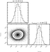 |
Fig. B.1 Marginalized distributions of m and tcentered. These are obtained after centering all datasets by normalizing with the mean NOH and |


Appendix C Individual sources – transitions of the OH ground state
This appendix shows the spectra of the OH ground state transitions.
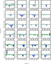 |
Fig. C.1 Spectra of OH ground state transitions, especially also of the satellite lines, along lines of sight that show a detection in 1665 or 1667 MHz absorption. The spectra are extracted from data cubes that have been smoothed to 46′′ resolution. The transitions at 1665 MHz (black), 1612 MHz (orange), and 1720 MHz (cyan) are shown for all sources. The 1667 MHz (green) transition is displayed if available. OH absorption detections in the main line transitions are shaded in blue. |
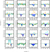 |
Fig. C.1 continued. |
Appendix D Individual sources – OH and H I optical depth and 13CO(1−0) emission
The appendix shows the OH and H I optical depth profiles for each source, as well as the 13CO(1–0) emission.
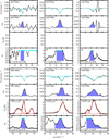 |
Fig. D.1 Analyzed 1665 and 1667 MHz OH absorption features. Topmost panel: 1665 MHz (black) and 1667 MHz (green) absorption features. Second panel from the top: spectrum converted to optical depth for the 1665 MHz (black) and 1667 MHz (green) transition. Third panel from the top: 13CO (1−0) emission in Tmb (data from the GRS survey (l < 60°) and Exeter FCRAO CO survey (l > 60°); Jackson et al. 2006, Mottram & Brunt 2010). The line widths were determined by fitting Gaussian profiles to the 1665 MHz (cyan) and 1667 MHz (orange) absorption, and the 13CO (1−0) emission (red). Lowermost panel: H I absorption converted to H I optical depth. Measured bins are denoted by black dots, while we quote lower limits (cyan) for saturated bins. The 1667 MHz transition was observed only towards selected regions and is therefore shown only for a subset of lines-of-sight (see Sect. 2). Theline-of-sight coordinates are given in degrees of Galactic coordinates. The blue shaded area in the lower three panels shows the line integrals. All data were smoothed to a spatial resolution of 46′′. |
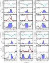 |
Fig. D.2 continued. |
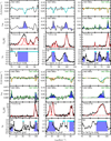 |
Fig. D.2 continued. |
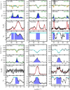 |
Fig. D.2 continued. |
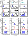 |
Fig. D.2 continued. |
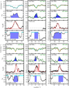 |
Fig. D.2 continued. |
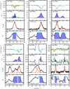 |
Fig. D.2 continued. |
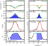 |
Fig. D.2 continued. |
Appendix E OH absorption towards W43
Moment zero map of the optical depth of the 1667 MHz transition for different velocity intervals towards W43.
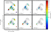 |
Fig. E.1 Integrated optical depth of the OH 1667 MHz line in the W43 star-forming region. In the top-left panel, τ is integrated over the same velocity range as in Fig. 10. The other panels show τ around the indicated velocities after integrating over three channels of 1.5 km s−1 width. For each pixel, only channels that are detected at a 3σ level or higher contribute to the integrated τ-map. The optical depth map is overlayed with contours of the 18 cm continuum emission (black, in levels of 0.1, 0.2, 0.4, 0.6, 0.8, 1.0, 1.25, 1.5, and 1.75 Jy beam−1). Symbols as in Fig. 10. |
References
- Allen, R. J., Hogg, D. E., & Engelke, P. D. 2015, AJ, 149, 123 [NASA ADS] [CrossRef] [Google Scholar]
- Anderson, L. D., Bania, T. M., Jackson, J. M., et al. 2009, ApJS, 181, 255 [NASA ADS] [CrossRef] [Google Scholar]
- Anderson, L. D., Bania, T. M., Balser, D. S., et al. 2014, ApJS, 212, 1 [NASA ADS] [CrossRef] [Google Scholar]
- Argon, A. L., Reid, M. J., & Menten, K. M. 2000, ApJS, 129, 159 [NASA ADS] [CrossRef] [Google Scholar]
- Astropy Collaboration, Robitaille, T. P., Tollerud, E. J., et al. 2013, A&A, 558, A33 [NASA ADS] [CrossRef] [EDP Sciences] [Google Scholar]
- Bally, J., Anderson, L. D., Battersby, C., et al. 2010, A&A, 518, L90 [Google Scholar]
- Balser, D. S., Goss, W. M., & De Pree C. G. 2001, AJ, 121, 371 [NASA ADS] [CrossRef] [Google Scholar]
- Beuther, H., Tackenberg, J., Linz, H., et al. 2012, A&A, 538, A11 [NASA ADS] [CrossRef] [EDP Sciences] [Google Scholar]
- Beuther, H., Bihr, S., Rugel, M., et al. 2016, A&A, 595, A32 [NASA ADS] [CrossRef] [EDP Sciences] [Google Scholar]
- Bialy, S., Bihr, S., Beuther, H., Henning, T., & Sternberg, A. 2017, ApJ, 835, 126 [NASA ADS] [CrossRef] [Google Scholar]
- Bihr, S., Beuther, H., Ott, J., et al. 2015, A&A, 580, A112 [NASA ADS] [CrossRef] [EDP Sciences] [Google Scholar]
- Bihr, S., Johnston, K. G., Beuther, H., et al. 2016, A&A, 588, A97 [NASA ADS] [CrossRef] [EDP Sciences] [Google Scholar]
- Blaauw, A., Gum, C. S., Pawsey, J. L., & Westerhout, G. 1960, MNRAS, 121, 123 [NASA ADS] [CrossRef] [Google Scholar]
- Blum, R. D., Damineli, A., & Conti, P. S. 1999, AJ, 117, 1392 [NASA ADS] [CrossRef] [Google Scholar]
- Bohlin, R. C., Savage, B. D., & Drake, J. F. 1978, ApJ, 224, 132 [NASA ADS] [CrossRef] [Google Scholar]
- Bolatto, A. D., Wolfire, M., & Leroy, A. K. 2013, ARA&A, 51, 207 [Google Scholar]
- Bourke, T. L., Myers, P. C., Robinson, G., & Hyland, A. R. 2001, ApJ, 554, 916 [NASA ADS] [CrossRef] [Google Scholar]
- Brooks, K. J., & Whiteoak, J. B. 2001, MNRAS, 320, 465 [NASA ADS] [CrossRef] [Google Scholar]
- Carlhoff, P., Nguyen Luong, Q., Schilke, P., et al. 2013, A&A, 560, A24 [NASA ADS] [CrossRef] [EDP Sciences] [Google Scholar]
- Cesaroni, R., & Walmsley, C. M. 1991, A&A, 241, 537 [NASA ADS] [Google Scholar]
- Colgan, S. W. J., Salpeter, E. E., & Terzian, Y. 1989, ApJ, 336, 231 [NASA ADS] [CrossRef] [Google Scholar]
- Contreras, Y., Schuller, F., Urquhart, J. S., et al. 2013, A&A, 549, A45 [NASA ADS] [CrossRef] [EDP Sciences] [Google Scholar]
- Crutcher, R. M. 1977, ApJ, 216, 308 [NASA ADS] [CrossRef] [Google Scholar]
- Crutcher, R. M. 1979, ApJ, 234, 881 [NASA ADS] [CrossRef] [Google Scholar]
- Csengeri, T., Menten, K. M., Wyrowski, F., et al. 2012, A&A, 542, L8 [NASA ADS] [CrossRef] [EDP Sciences] [Google Scholar]
- Dawson, J. R., Walsh, A. J., Jones, P. A., et al. 2014, MNRAS, 439, 1596 [NASA ADS] [CrossRef] [Google Scholar]
- Dickey, J. M., Crovisier, J., & Kazes, I. 1981, A&A, 98, 271 [NASA ADS] [Google Scholar]
- Dobbs, C. L., Krumholz, M. R., Ballesteros-Paredes, J., et al. 2014, in Protostars and Planets VI, eds. H. Beuther, R. S. Klessen, C. P. Dullemond, & T. Henning (Tucson: Univ. of Arizona Press), 3 [Google Scholar]
- Ebisawa, Y., Inokuma, H., Sakai, N., et al. 2015, ApJ, 815, 13 [NASA ADS] [CrossRef] [Google Scholar]
- Elitzur, M. 1992, Astronomical Masers (Dordrecht: Kluwer Academic Publishers), Astrophys. Space Sci. Lib., 170 [Google Scholar]
- Frayer, D. T., Seaquist, E. R., & Frail, D. A. 1998, AJ, 115, 559 [NASA ADS] [CrossRef] [Google Scholar]
- Frerking, M. A., Langer, W. D., & Wilson, R. W. 1982, ApJ, 262, 590 [NASA ADS] [CrossRef] [Google Scholar]
- Ginsburg, A., Bressert, E., Bally, J., & Battersby, C. 2012, ApJ, 758, L29 [NASA ADS] [CrossRef] [Google Scholar]
- Goodman, A. A., Alves, J., Beaumont, C. N., et al. 2014, ApJ, 797, 53 [NASA ADS] [CrossRef] [Google Scholar]
- Goss, W. M. 1968, ApJS, 15, 131 [NASA ADS] [CrossRef] [Google Scholar]
- Grenier, I. A., Casandjian, J.-M., & Terrier, R. 2005, Science, 307, 1292 [NASA ADS] [CrossRef] [PubMed] [Google Scholar]
- Guelin, M. 1985, in Molecular Astrophysics: State of the Art and Future Directions, eds. G. H. F. Diercksen, W. F. Huebner, & P. W. Langhoff (Dordrecht: D. Reidel Publishing), 23 [Google Scholar]
- Guibert, J., Rieu, N. Q., & Elitzur, M. 1978, A&A, 66, 395 [NASA ADS] [Google Scholar]
- Hales, C. A., Murphy, T., Curran, J. R., et al. 2012, MNRAS, 425, 979 [NASA ADS] [CrossRef] [Google Scholar]
- Heiles, C., Goodman, A. A., McKee, C. F., & Zweibel, E. G. 1993, in Protostars and Planets III, eds. E. H. Levy, & J. I. Lunine, 279 [Google Scholar]
- Heyer, M., & Dame, T. M. 2015, ARA&A, 53, 583 [NASA ADS] [CrossRef] [Google Scholar]
- Hollenbach, D., Kaufman, M. J., Bergin, E. A., & Melnick, G. J. 2009, ApJ, 690, 1497 [CrossRef] [Google Scholar]
- Hollenbach, D., Kaufman, M. J., Neufeld, D., Wolfire, M., & Goicoechea, J. R. 2012, ApJ, 754, 105 [NASA ADS] [CrossRef] [Google Scholar]
- Jackson, J. M., Rathborne, J. M., Shah, R. Y., et al. 2006, ApJS, 163, 145 [NASA ADS] [CrossRef] [Google Scholar]
- Klessen, R. S., & Glover, S. C. O. 2016, in Physical Processes in the Interstellar Medium, eds. Y. Revaz, P. Jablonka, R. Teyssier, & L. Mayer (Berlin: Springer-Verlag), 43, 85 [Google Scholar]
- Langer, W. D., & Graedel, T. E. 1989, ApJS, 69, 241 [NASA ADS] [CrossRef] [Google Scholar]
- Lester, D. F., Dinerstein, H. L., Werner, M. W., et al. 1985, ApJ, 296, 565 [NASA ADS] [CrossRef] [Google Scholar]
- Li, D., & Goldsmith, P. F. 2003, ApJ, 585, 823 [NASA ADS] [CrossRef] [Google Scholar]
- Li, D., Tang, N., Nguyen, H., et al. 2018, ApJS, 235, 1 [NASA ADS] [CrossRef] [Google Scholar]
- Liszt, H. S. 1995, AJ, 109, 1204 [NASA ADS] [CrossRef] [Google Scholar]
- Liszt, H., & Lucas, R. 1996, A&A, 314, 917 [NASA ADS] [Google Scholar]
- Liszt, H., & Lucas, R. 1999, in Highly Redshifted Radio Lines, eds. C. L. Carilli, S. J. E. Radford, K. M. Menten, & G. I. Langston, ASP Conf. Ser., 156, 188 [NASA ADS] [Google Scholar]
- Liszt, H., & Lucas, R. 2002, A&A, 391, 693 [NASA ADS] [CrossRef] [EDP Sciences] [Google Scholar]
- Louvet, F., Motte, F., Gusdorf, A., et al. 2016, A&A, 595, A122 [NASA ADS] [CrossRef] [EDP Sciences] [Google Scholar]
- McKee, C. F., & Ostriker, E. C. 2007, ARA&A, 45, 565 [NASA ADS] [CrossRef] [Google Scholar]
- Milam, S. N., Savage, C., Brewster, M. A., Ziurys, L. M., & Wyckoff, S. 2005, ApJ, 634, 1126 [NASA ADS] [CrossRef] [Google Scholar]
- Miville-Deschênes, M.-A., Murray, N., & Lee, E. J. 2017, ApJ, 834, 57 [NASA ADS] [CrossRef] [Google Scholar]
- Motte, F., Schilke, P., & Lis, D. C. 2003, ApJ, 582, 277 [NASA ADS] [CrossRef] [Google Scholar]
- Motte, F., Nguyen Luong, Q., Schneider, N., et al. 2014, A&A, 571, A32 [NASA ADS] [CrossRef] [EDP Sciences] [Google Scholar]
- Mottram, J. C., & Brunt, C. M. 2010, in The Dynamic Interstellar Medium: A Celebration of the Canadian Galactic Plane Survey, eds. R. Kothes, T. L. Landecker, & A. G. Willis, ASP Conf. Ser., 438, 98 [NASA ADS] [Google Scholar]
- Neufeld, D. A., Kaufman, M. J., Goldsmith, P. F., Hollenbach, D. J., & Plume, R. 2002, ApJ, 580, 278 [NASA ADS] [CrossRef] [Google Scholar]
- Nguyen-Luong, Q., Motte, F., Schuller, F., et al. 2011, A&A, 529, A41 [NASA ADS] [CrossRef] [EDP Sciences] [Google Scholar]
- Nguyen-Luong, Q., Motte, F., Carlhoff, P., et al. 2013, ApJ, 775, 88 [NASA ADS] [CrossRef] [Google Scholar]
- Nguyen-Luong, Q., Anderson, L. D., Motte, F., et al. 2017, ApJ, 844, L25 [NASA ADS] [CrossRef] [Google Scholar]
- Nishimura, A., Tokuda, K., Kimura, K., et al. 2015, ApJS, 216, 18 [NASA ADS] [CrossRef] [EDP Sciences] [Google Scholar]
- Offer, A., van Hemert, M., & van Dishoeck, E. 1994, J. Chem. Phys., 100, 362 [NASA ADS] [CrossRef] [Google Scholar]
- Phillips, T. G., Knapp, G. R., Wannier, P. G., et al. 1981, ApJ, 245, 512 [NASA ADS] [CrossRef] [Google Scholar]
- Pihlström, Y. M., Fish, V. L., Sjouwerman, L. O., et al. 2008, ApJ, 676, 371 [NASA ADS] [CrossRef] [Google Scholar]
- Pineda, J. E., Caselli, P., & Goodman, A. A. 2008, ApJ, 679, 481 [NASA ADS] [CrossRef] [Google Scholar]
- Pineda, J. L., Goldsmith, P. F., Chapman, N., et al. 2010, ApJ, 721, 686 [NASA ADS] [CrossRef] [Google Scholar]
- Pineda, J. L., Langer, W. D., Velusamy, T., & Goldsmith, P. F. 2013, A&A, 554, A103 [NASA ADS] [CrossRef] [EDP Sciences] [Google Scholar]
- Planck Collaboration XIX. 2011, A&A, 536, A19 [NASA ADS] [CrossRef] [EDP Sciences] [Google Scholar]
- Ragan, S. E., Henning, T., Tackenberg, J., et al. 2014, A&A, 568, A73 [NASA ADS] [CrossRef] [EDP Sciences] [Google Scholar]
- Reid, M. J., Menten, K. M., Brunthaler, A., et al. 2014, ApJ, 783, 130 [Google Scholar]
- Reifenstein, E. C., Wilson, T. L., Burke, B. F., Mezger, P. G., & Altenhoff, W. J. 1970, A&A, 4, 357 [NASA ADS] [Google Scholar]
- Schöier, F. L., van der Tak, F. F. S., van Dishoeck, E. F., & Black, J. H. 2005, A&A, 432, 369 [NASA ADS] [CrossRef] [EDP Sciences] [Google Scholar]
- Schuller, F., Menten, K. M., Contreras, Y., et al. 2009, A&A, 504, 415 [NASA ADS] [CrossRef] [EDP Sciences] [Google Scholar]
- Smith, L. F., Biermann, P., & Mezger, P. G. 1978, A&A, 66, 65 [NASA ADS] [Google Scholar]
- Smith, R. J., Glover, S. C. O., Clark, P. C., Klessen, R. S., & Springel, V. 2014, MNRAS, 441, 1628 [NASA ADS] [CrossRef] [Google Scholar]
- Snow, T. P. & McCall, B. J. 2006, ARA&A, 44, 367 [NASA ADS] [CrossRef] [Google Scholar]
- Stanimirović, S., Weisberg, J. M., Dickey, J. M., et al. 2003, ApJ, 592, 953 [NASA ADS] [CrossRef] [Google Scholar]
- Stil, J. M., Taylor, A. R., Dickey, J. M., et al. 2006, AJ, 132, 1158 [NASA ADS] [CrossRef] [Google Scholar]
- Szűcs, L., Glover, S. C. O., & Klessen, R. S. 2016, MNRAS, 460, 82 [NASA ADS] [CrossRef] [Google Scholar]
- Tang, N., Li, D., Heiles, C., et al. 2017, ApJ, 839, 8 [NASA ADS] [CrossRef] [Google Scholar]
- Turner, B. E. 1966, Nature, 212, 184 [NASA ADS] [CrossRef] [Google Scholar]
- Turner, B. E. 1973, ApJ, 186, 357 [NASA ADS] [CrossRef] [Google Scholar]
- Turner, B. E. 1979, A&AS, 37, 1 [NASA ADS] [Google Scholar]
- Turner, B. E.,& Heiles, C. 1971, ApJ, 170, 453 [NASA ADS] [CrossRef] [Google Scholar]
- Urquhart, J. S., Thompson, M. A., Moore, T. J. T., et al. 2013, MNRAS, 435, 400 [NASA ADS] [CrossRef] [Google Scholar]
- Urquhart, J. S., Csengeri, T., Wyrowski, F., et al. 2014, A&A, 568, A41 [NASA ADS] [CrossRef] [EDP Sciences] [Google Scholar]
- van Dishoeck, E. F., Herbst, E., & Neufeld, D. A. 2013, Chem. Rev., 113, 9043 [NASA ADS] [CrossRef] [PubMed] [Google Scholar]
- van Langevelde, H. J., van Dishoeck, E. F., Sevenster, M. N., & Israel, F. P. 1995, ApJ, 448, L123 [NASA ADS] [CrossRef] [Google Scholar]
- Walsh, A. J., Beuther, H., Bihr, S., et al. 2016, MNRAS, 455, 3494 [NASA ADS] [CrossRef] [Google Scholar]
- Wang, Y., Bihr, S., Rugel, M., et al., 2018, A&A, in press, DOI: 10.1051/0004-6361/201833642 [Google Scholar]
- Wannier, P. G., Andersson, B.-G., Federman, S. R., et al. 1993, ApJ, 407, 163 [NASA ADS] [CrossRef] [Google Scholar]
- Weinreb, S., Barrett, A. H., Meeks, M. L., & Henry, J. C. 1963, Nature, 200, 829 [NASA ADS] [CrossRef] [Google Scholar]
- Weselak, T., Galazutdinov, G. A., Beletsky, Y., & Krełowski, J. 2010, MNRAS, 402, 1991 [NASA ADS] [CrossRef] [Google Scholar]
- Wiesemeyer, H., Güsten, R., Heyminck, S., et al. 2012, A&A, 542, L7 [NASA ADS] [CrossRef] [EDP Sciences] [Google Scholar]
- Wiesemeyer, H., Güsten, R., Heyminck, S., et al. 2016, A&A, 585, A76 [NASA ADS] [CrossRef] [EDP Sciences] [Google Scholar]
- Wilson, T. L., Rohlfs, K., & Hüttemeister, S. 2009, Tools of Radio Astronomy (Berlin: Springer-Verlag) [Google Scholar]
- Xu, D., Li, D., Yue, N., & Goldsmith, P. F. 2016, ApJ, 819, 22 [NASA ADS] [CrossRef] [Google Scholar]
- Yusef-Zadeh, F., Wardle, M., & Roberts, D. A. 2003, ApJ, 583, 267 [NASA ADS] [CrossRef] [Google Scholar]
- Zhang, B., Moscadelli, L., Sato, M., et al. 2014, ApJ, 781, 89 [NASA ADS] [CrossRef] [Google Scholar]
http://casa.nrao.edu; version 4.2.2.
This sample of 15 datapoints is described by a Pearson’s correlation coefficient ρ = 0.8 at a statistical significance of ≈3σ.
Assuming NH∕(AV∕RV) = 5.8 × 1021 cm−2 mag−1 (Bohlin et al. 1978) and the average ISM value for the total-to-selective extinction of RV = 3.1, the total hydrogen column density can be related to visual extinction as NH = 1.9 × 1021 cm−2 mag−1 × AV. For large column densities ( ) we assume the contribution of atomic hydrogen to be negligible, i.e.,
  .
.
All Tables
Derived quantities from OH 1665/1667 MHz and H I absorption and 13CO(1–0) emission.
All Figures
|
Fig. 1 Example spectra and optical depths at l = +29.935°, b = −0.053° (at 46″ resolution). Topmost two panels: 1665 and 1667 MHz absorption features. The fitted Gaussian profiles for the 1665 MHz line (cyan) and 1667 MHz line (orange) are overlaid. Two middle panels: optical depth of the 1665 and 1667 MHz transitions. Second panel from the bottom: emission of 13CO (1–0) in main-beam temperature (Tmb), overlaid with a fitted Gaussian profile (red). Lowermost panel: H I optical depth as measured from the absorption spectra. Lower limits (cyan dots) are given for saturated bins. The blue shaded area in the lower four panels denotes the area of the transitions, from which the column densities are determined. |
| In the text | |
|
Fig. 2 Detections of OH absorption at 1665 and 1667 MHz (red circles) overplotted on continuum emission at 1.4 GHz from the combined THOR and VGPS data (Beuther et al. 2016; Wang et al. 2018). |
| In the text | |
|
Fig. 3 Peak optical depth of the 1665-MHz transition (circles) and the 1667-MHz transition (crosses) vs. continuum flux density at 46′′. The sensitivity in OH optical depth is indicated by an average 4σ detection limit (black dashed curve). Variations in the detection limit among sightlines are indicated by the gray shaded area. |
| In the text | |
|
Fig. 4 Number of continuum sources with OH absorption detections vs. Galactic latitude. |
| In the text | |
|
Fig. 5 Number of continuum sources with OH absorption detections vs. Galactic longitude. The 1665 MHz transition was observed over the entire region of the survey. The coverage of the 1667 MHz transition is indicated by the black bars. |
| In the text | |
|
Fig. 6 Comparison of FWHM of OH and 13CO(1–0) lines. OH line widths of the 1665 MHz transition (squares) are used whenever the 1667 MHz transition (circles) was not available. Detections associated with H II regions are drawn in black, others in red. Arrows indicate spectrally unresolved lines. The dashed line indicates a 1:1 correlation. The bars in the lower right-hand corner of the figure indicate typical errors in both quantities. |
| In the text | |
|
Fig. 7 Comparison of the OH column density from the 1665 MHz (squares) and 1667 MHz transitions (circles) to that of H2 as inferred from 13CO(1–0) emission. Column densities from absorption features overlapping in velocity with H II regions (black) and with no such counterpart (red) divide the plot into regions with higher and lower hydrogen column densities. Triangles denote upper limits on |
| In the text | |
|
Fig. 8 OH abundance |
| In the text | |
|
Fig. 9 OH abundance XOH = NOH∕NH vs. NH. The total column density of hydrogen nuclei, NH, is inferred from 13CO(1–0) emission and H I absorption. As the H I column density represents lower limits, the OH abundances represent upper limits. Colors and symbols are as in Fig. 8. The right axis shows the OH abundance in units of the typical OH abundance in diffuse clouds of 4 × 10⁻⁸ (Crutcher 1979, indicated also by the dashed gray line). |
| In the text | |
|
Fig. 10 Comparison of τ(OH 1667 MHz), dust continuum emission at λ = 870 μm, and C18 O(2–1) emission in the W43 star-forming region. In the left panel, the integrated optical depth of the OH 1667 MHz transition between 78.0and 100.5 km s−1 is displayed in colors. For each pixel, only channels that are detected at a 3σ level contribute to the integrated τ-map. It is overlayed with contours of the 18 cm continuum emission (black, at levels of 0.1, 0.2, 0.4, 0.6, 0.8, 1.0, 1.25, 1.5 and 1.75 Jy beam−1). Middle panel: ratio of the integrated τ(OH) map to 870 μm ATLASGAL emission (Schuller et al. 2009), which traces dense gas (the dust emission is overlayed in black contours, at levels of 0.5, 1.0, 2.0, 3.0, 4.0, 5.0, 7.0 and 10.0 Jy beam−1). Right panel: ratio of τ(OH) to C18 O(2–1) emission (Carlhoff et al. 2013), integrated over the same velocity range (the velocity integrated C18 O(2–1) emission is overplotted in black contours at levels of 6, 9, 13, 15, 17, 19, 23 K km s −1). All data have been smoothed to a common resolution of 20′′, corresponding to spatial scales of 0.5 pc. In the left panel, the central Wolf–Rayet/OB cluster is marked by a black star, while the dense clumps MM1 and MM3 (Motte et al. 2003) are marked by blue stars. The upper end of the T-bar-shaped continuum emission is marked as Pos. 1 for easier reference in the text. For readability, the values of the ratio are displayed for selected positions in the figure. |
| In the text | |
|
Fig. 11 Ratio of integrated τ(OH 1667 MHz) absorption and C18O(2–1) emission in W43. The top-left panel is the same as the rightmost panel in Fig. 10 and is shown for orientation. The other panels show the ratio of τ(OH 1667 MHz) and C18 O(2–1) at the indicated velocities after binning three channels of 1.5 km s−1 width. Overlayed on all panels are contours of 18 cm continuum emission (black, in levels of 0.1, 0.2, 0.4, 0.6, 0.8, 1.0, 1.25, 1.5 and 1.75 Jy beam−1). The 1667 MHz optical depth has been masked at 3σ detection levels in the original OH absorption data. For pixels with no C18O emission counterpart, 3σ detection limits have been used, and are indicated by blue contours. The ratio is quoted in brackets for these locations. |
| In the text | |
|
Fig. 12 Spectra of τOH in the 1665 and 1667 MHz lines, as well as of emission in C18O(2–1) line. The spectra are extracted towards positions MM1, MM36, WR and “Pos. 1” as indicated in Figs. 10 and 11, as well as towards the central part of the T-bar. Towards MM3, the channel at 96 km s −1 of the OH 1667MHz absorption is masked because of sidelobes of close-by maser emission. |
| In the text | |
|
Fig. 13 Comparison of the OH molecular abundances from this work to abundances measured in Wiesemeyer et al. (2016). Data, symbols and systematic uncertainties as in Fig. 8. Measurements from Table 4 of Wiesemeyer et al. (2016) are overplotted as purple diamonds. Filled diamonds use HF as proxy for the H2 column density. Empty diamonds use CH. If both HF and CH measurements are available, OH measurements are drawn twice. Black diagonal lines indicate sensitivity limits of XOH for typical 4σ limits on optical depth in the OH main lines and assuming a line width of 2.5 km s −1 (the detection limits of τ = 0.025, 0.05 and 0.1 are acchieved for continuum sources stronger than Fcont = 2.10, 1.05 and 0.53 Jy beam−1, respectively). |
| In the text | |
|
Fig. B.1 Marginalized distributions of m and tcentered. These are obtained after centering all datasets by normalizing with the mean NOH and |
| In the text | |
|
Fig. C.1 Spectra of OH ground state transitions, especially also of the satellite lines, along lines of sight that show a detection in 1665 or 1667 MHz absorption. The spectra are extracted from data cubes that have been smoothed to 46′′ resolution. The transitions at 1665 MHz (black), 1612 MHz (orange), and 1720 MHz (cyan) are shown for all sources. The 1667 MHz (green) transition is displayed if available. OH absorption detections in the main line transitions are shaded in blue. |
| In the text | |
|
Fig. C.1 continued. |
| In the text | |
|
Fig. D.1 Analyzed 1665 and 1667 MHz OH absorption features. Topmost panel: 1665 MHz (black) and 1667 MHz (green) absorption features. Second panel from the top: spectrum converted to optical depth for the 1665 MHz (black) and 1667 MHz (green) transition. Third panel from the top: 13CO (1−0) emission in Tmb (data from the GRS survey (l < 60°) and Exeter FCRAO CO survey (l > 60°); Jackson et al. 2006, Mottram & Brunt 2010). The line widths were determined by fitting Gaussian profiles to the 1665 MHz (cyan) and 1667 MHz (orange) absorption, and the 13CO (1−0) emission (red). Lowermost panel: H I absorption converted to H I optical depth. Measured bins are denoted by black dots, while we quote lower limits (cyan) for saturated bins. The 1667 MHz transition was observed only towards selected regions and is therefore shown only for a subset of lines-of-sight (see Sect. 2). Theline-of-sight coordinates are given in degrees of Galactic coordinates. The blue shaded area in the lower three panels shows the line integrals. All data were smoothed to a spatial resolution of 46′′. |
| In the text | |
|
Fig. D.2 continued. |
| In the text | |
|
Fig. D.2 continued. |
| In the text | |
|
Fig. D.2 continued. |
| In the text | |
|
Fig. D.2 continued. |
| In the text | |
|
Fig. D.2 continued. |
| In the text | |
|
Fig. D.2 continued. |
| In the text | |
|
Fig. D.2 continued. |
| In the text | |
|
Fig. E.1 Integrated optical depth of the OH 1667 MHz line in the W43 star-forming region. In the top-left panel, τ is integrated over the same velocity range as in Fig. 10. The other panels show τ around the indicated velocities after integrating over three channels of 1.5 km s−1 width. For each pixel, only channels that are detected at a 3σ level or higher contribute to the integrated τ-map. The optical depth map is overlayed with contours of the 18 cm continuum emission (black, in levels of 0.1, 0.2, 0.4, 0.6, 0.8, 1.0, 1.25, 1.5, and 1.75 Jy beam−1). Symbols as in Fig. 10. |
| In the text | |
Current usage metrics show cumulative count of Article Views (full-text article views including HTML views, PDF and ePub downloads, according to the available data) and Abstracts Views on Vision4Press platform.
Data correspond to usage on the plateform after 2015. The current usage metrics is available 48-96 hours after online publication and is updated daily on week days.
Initial download of the metrics may take a while.