| Issue |
A&A
Volume 617, September 2018
|
|
|---|---|---|
| Article Number | A89 | |
| Number of page(s) | 17 | |
| Section | Interstellar and circumstellar matter | |
| DOI | https://doi.org/10.1051/0004-6361/201832753 | |
| Published online | 21 September 2018 | |
Search for high-mass protostars with ALMA revealed up to kilo-parsec scales (SPARKS)
I. Indication for a centrifugal barrier in the environment of a single high-mass envelope★
1
Max-Planck-Institut für Radioastronomie,
Auf dem Hügel 69,
53121
Bonn,
Germany
e-mail: This email address is being protected from spambots. You need JavaScript enabled to view it.
2
OASU/LAB-UMR5804, CNRS, Université Bordeaux, Allée Geoffroy Saint-Hilaire,
33615
Pessac, France
3
INAF – Osservatorio Astronomico di Cagliari,
Via della Scienza 5,
09047
Selargius (CA), Italy
4
Max- Planck Institute for Astronomy,
Königstuhl 17,
69117
Heidelberg, Germany
5
Departamento de Astronomía, Universidad de Chile,
Casilla 36-D,
Santiago, Chile
6
ENS de Lyon, Univ Lyon 1, CNRS, Centre de Recherche Astrophysique de Lyon UMR5574, Université de Lyon,
69007
Lyon, France
7
IRAM,
300 Rue de la piscine,
38406
Saint-Martin-d’Hères, France
8
Astrophysics Research Institute, Liverpool John Moores University,
Liverpool
L3 5RF, UK
9
Instituto de Radioastronomía y Astrofísica, Universidad Nacional Autónoma de Mexico,
PO Box 3-72,
58090
Morelia,
Michoacán, Mexico
10
Department of Space, Earth & Environment, Chalmers University of Technology,
Gothenburg, Sweden
11
Department of Astronomy, University of Virginia,
Charlottesville,
VA 22904-4325, USA
12
School of Physical Sciences, University of Kent, Ingram Building,
Canterbury, Kent
CT2 7NH, UK
Received:
2
February
2018
Accepted:
28
May
2018
Abstract
The conditions leading to the formation of the most massive O-type stars are still an enigma in modern astrophysics. To assess the physical conditions of high-mass protostars in their main accretion phase, here we present a case study of a young massive clump selected from the ATLASGAL survey, G328.2551–0.5321. The source exhibits a bolometric luminosity of 1.3 × 10⁴ L⊙, which allows us to estimate that its current protostellar mass lies between ~11 and 16 M⊙. We show high angular resolution observations with ALMA that reach a physical scale of ~400 au. To reveal the structure of this high-mass protostellar envelope in detail at a ~0.17′′ resolution, we used the thermal dust continuum emission and spectroscopic information, amongst others from the CO (J = 3–2) line, which is sensitive to the high-velocity molecular outflow of the source. We also used the SiO (J = 8–7) and SO2 (J = 82,6 − 71,7) lines, which trace shocks along the outflow, as well as several CH3OH and HC3N lines that probe the gas of the inner envelope in the closest vicinity of the protostar. Our observations of the dust continuum emission reveal a single high-mass protostellar envelope, down to our resolution limit. We find evidence for a compact, marginally resolved continuum source that is surrounded by azimuthal elongations that could be consistent with a spiral pattern. We also report on the detection of a rotational line of CH3OH within its vt = 1 torsionally excited state. This shows two bright emission peaks that are spatially offset from the dust continuum peak and exhibit a distinct velocity component ±4.5 km s−1 offset from the systemic velocity of the source. Rotational diagram analysis and models based on local thermodynamic equilibrium assumption require high CH3OH column densities that reach N(CH3OH) = 1.2−2 × 1019 cm−2, and kinetic temperatures of the order of 160–200 K at the position of these peaks. A comparison of their morphology and kinematics with those of the outflow component of the CO line and the SO2 line suggests that the high-excitation CH3OH spots are associated with the innermost regions of the envelope. While the HC3N v7 = 0 (J = 37–36) line is also detected in the outflow, the HC3N v7 = 1e (J = 38–37) rotational transition within the first vibrationally excited state of the molecule shows a compact morphology. We find that the velocity shifts at the position of the observed high-excitation CH3 OH spots correspond well to the expected Keplerian velocity around a central object with 15 M⊙ consistent with the mass estimate based on the bolometric luminosity of the source. We propose a picture where the CH3 OH emission peaks trace the accretion shocks around the centrifugal barrier, pinpointing the interaction region between the collapsing envelope and an accretion disc. The physical properties of the accretion disc inferred from these observations suggest a specific angular momentum several times higher than typically observed towards low-mass protostars. This is consistent with a scenario of global collapse setting on at larger scales that could carry a more significant amount of kinetic energy compared to the core-collapse models of low-mass star formation. Furthermore, our results suggest that vibrationally excited HC3 N emission could be a new tracer for compact accretion discs around high-mass protostars.
Key words: accretion, accretion disks / stars: massive / stars: formation / submillimeter: ISM
The reduced datacubes are only available at the CDS via anonymous ftp to cdsarc.u-strasbg.fr (130.79.128.5) or via http://cdsarc.u-strasbg.fr/viz-bin/qcat?J/A+A/617/A89
© ESO 2018
1 Introduction
Whether high-mass star formation proceeds as a scaled-up version of low-mass star formation is an open question in today’s astrophysics. Signatures of infall and accretion processes associated with the formation of high-mass stars are frequently observed: ejection of material (Beuther et al. 2002; Zhang et al. 2005; Beltrán et al. 2011; Duarte-Cabral et al. 2013) with powerful jets (Guzmán et al. 2010; Moscadelli et al. 2016; Purser et al. 2016) and the existence of (massive) rotating structures, such as toroids and discs, have been reported towards massive young stellar objects (MYSOs; Beltrán et al. 2005; Sanna et al. 2015; Cesaroni et al. 2017). Most of these studies, however, focus on sources with high luminosities (Lbol > 3 × 10⁴ L⊙) that are frequently associated with at least one embedded UC H II region (see also Mottram et al. 2011). Some of them harbour already formed O-type YSOs that are typically accompanied by radio emission and surrounded by hot molecular, as well as ionised gas. Some examples are G23.01–00.41 (Sanna et al. 2015), G35.20–0.74N (Sánchez-Monge et al. 2013), and G345.4938+01.4677 (also known as IRAS 16562–3959; Guzmán et al. 2014), which have been studied in detail at high angular resolution.
High-mass star formation activity is typically accompanied by the emergence of radio continuum emission (Rosero et al. 2016). The earlier evolutionary stage of high-mass star formation that precedes the emergence of strong ionising radiation from an UC-HII region is characterised by typically lower bolometric luminosity (e.g. Molinari et al. 2000; Sridharan et al. 2002; Motte et al. 2007). This stage can be considered as an analogue of the Class 0 stage of low-mass protostars (Duarte-Cabral et al. 2013), which could be the main accretion phase, dominated by the cold and dusty envelope, and is accompanied by powerful ejection of material (Bontemps et al. 1996; André et al. 2000). Owing to the high column densities, extinction is very high towards these objects, and therefore high-mass protostars in this early stage are elusive (e.g. Bontemps et al. 2010; Motte et al. 2018). Rare examples of them are found to be single down to ~500 au scales. They typically only probe a limited mass range: one of the best-studied sources is the protostar CygX-N63, which with a current envelope mass of ~55 M⊙ likely forms a star with a mass of ≲20 M⊙ (Bontemps et al. 2010; Duarte-Cabral et al. 2013).
We report here on the discovery of a single high-mass protostellar envelope with the highest mass observed so far, reaching the 100M⊙ mass range on 0.06 pc scale, which is expected to form a star with a mass of ~50 M⊙, corresponding to an O5–O4 type star. We resolve its immediate surroundings using high angular resolution observations that reach ~400 au with the Atacama Large Millimeter/submillimeter Array (ALMA). The observations show evidence for a flattened, rotating envelope, and accretion shocks, which implies the presence of a disc at a few hundred au scales.
2 Observations and data reduction
We study the mid-infrared quiet massive clump1, G328.2551– 0.5321, at high resolution. This source was selected from the complete sample of such sources, which was identified based on the APEX Telescope Large Area Survey of the Galaxy (ATLASGAL; Schuller et al. 2009; Csengeri et al. 2014, 2017a). The SPARKS project (Search for High-mass Protostars with ALMA up to kilo-parsec scales; Csengeri et al., in prep., a) targets 35 of these sources that correspond to the early evolutionary phase of high-mass star formation (Csengeri et al. 2017b). Located at a distance of 2.5 kpc, our target here is embedded in the MSXDC G328.25–00.51 dark cloud (Csengeri et al. 2017a). We show an overview of the region in the left panel of Fig. 1.
The source G328.2551–0.5321 has been observed with ALMA in Cycle 2, and the phase centre was  , − 53°57′57.8″). We used 11 of the 7 m antennas on 2014 July8 and 16, and 34−35 of the 12 m antennas on 2015 May 3, and 2015 September 1, respectively. The 7 m array observations are discussed in detail in Csengeri et al. (2017b). Here, we also present the 12 m array observations, whose baseline range is 15 m (17 kλ) to 1574 m (1809 kλ). The total time on source was 7.4 min, andthe system temperature (Tsys) varied between 120 and 200 K.
The spectral setups we used for the 7 and 12 m array observations are identical, and the signal was correlated in low-resolution wide-band mode in Band 7, yielding 4 × 1.75 GHz effective bandwidth with a spectral resolution of 0.977 MHz, which corresponds to ~0.9 km s−1 velocity resolution. The four basebands were centred on 347.331, 345.796, 337.061, and 333.900 GHz, respectively.
The data were calibrated in CASA 4.3.1 with the pipeline (version 34044). For the imaging, we used Briggs weighting with a robust parameter of − 2, corresponding to uniform weighting, favouring a smaller beam size, and we used the CLEAN algorithm for deconvolution. We created line-free continuum maps by excluding channels with line emission above 3σrms per channel determined on the brightest continuum source on the cleaned datacubes in an iterative process. The synthesised beam is 0.22′′ × 0.11′′, with a 86° position angle measured from north to east, which is the convention we follow from here on. The geometric mean of the major and minor axes corresponds to a beam size of 0.16′′ (~400 au at the adopted distance for the source).
To create cubes of molecular line emission, we subtracted the continuum determined in emission free channels around the selected line. To favour sensitivity, we used here a robust parameter of 0.5 for the imaging, which gives a synthesised beam of 0.34′′ × 0.20′′, with a geometric mean of 0.26′′ resolution (~650 au). For the SiO (8–7) datacube, we lowered the weight on the longest baselines with a tapering function to gain in signal-to-noise ratio. The resulting synthesised beam is 0.69′′ × 0.59′′ (corresponding to ~1600 au resolution).
We mainly focus here on molecular emission that originates from scales typically smaller than the largest angular scales of ~7′′, where the sensitivity of our 12 m array observations decreases. The interferometric filtering has, however, a significant effect on both the continuum and the CO (3–2) emission, which are considerably more extended than the largest angular scales probed by the ALMA configuration we used for these observations. For these two datasets, we therefore combined the 12 m array data with the data taken in the same setup with the 7 m array (Csengeri et al. 2017b). For this purpose, we used the standard procedures in CASA for a joint deconvolution, and imaged the data with a robust parameter of − 2, which provides the highest angular resolution. The resulting beam is 0.23×0.12′′ with a 86° position angle, with a geometric mean of 0.17′′ for the continuum maps, and 0.31×0.18′′ with an 88° position angle, with a geometric mean of 0.24′′ for the CO (3–2) line. We measure an rms noise level in the final continuum image of ~ 1.3 mJy beam−1 in an emission-free region close to the centre on the image corrected for primary beam attenuation. The primary beam of the 12 m array at this frequency is 18.′′ 5. To estimate the column density sensitivity, we used N(H2) =  , where Fν is the 3σrms flux density, Bν (T) is the Planck function, Ω is the solid angle of the beam calculated by Ω = 1.13 ×Θ2, where Θ is the geometric mean of the beam major and minor axes; κν = 0.0185 cm2 g−1 from Ossenkopf & Henning (1994) including the gas-to-dust ratio, R, of 100;
  is the meanmolecular weight per hydrogen molecule and is equal to 2.8; and mH is the mass of a hydrogen atom. For the mass estimation here and in the following, we used Eq. (2) from Csengeri et al. (2017a) with the parameters listed above. This gives us a 3σrms column density sensitivity of 2− 8× 1023 cm−2 for a physically motivated range of plausible temperatures corresponding to Td = 30−100 K, respectively, and within a beam size of 0.16′′, and a 5σ mass sensitivity of 0.03–0.13 M⊙ for the same temperature range.
 |
Fig. 1 Overview of the region centred on ℓ = +328.2551, b = −0.5321 in Galactic coordinates. Left panel: the three-colour composite image is from the Spitzer/GLIMPSE (Benjamin et al. 2003) and MIPSGAL (Carey et al. 2009) surveys (blue: 4.5 μm, green: 8 μm, and red: 24 μm) and is shownin Galactic coordinates. The contours show the 870 μm continuum emission from the ATLASGAL survey (Schuller et al. 2009; Csengeri et al. 2014). The arrow marks the dust continuum peak of the targeted clump, and the circle corresponds to the region shown in the right panel. Right panel: line-free continuum emission imaged at 345 GHz with the ALMA 12 m array. The colour scale is linear from − 3σ to 120σ. The contour shows the 7σ level. The FWHM size of the synthesised beam is shown in the lower left corner. |
3 Results
We discuss here the dust continuum image obtained with ALMA, which reveals a protostellar envelope, and a selected list of molecular tracers in order to study its protostellar activity and the kinematics of the gas in its close vicinity. From the total observed bandwidth of 7.5 GHz, we summarise the discussed transitions in Table 1. The full view of the molecular complexity of this source will be discussed in a forthcoming paper (Csengeri et al., in prep., b).
3.1 Dust continuum
3.1.1 Flattened envelope and compact dust continuum source
We show the line-free continuum emission of G328.2551–0.5321 in the right panel of Fig. 1, which reveals a single compact object down to 400 au physical scales. The source drives a prominent bipolar outflow (Sect. 3.4), suggesting that it hosts a protostar in its main accretion phase. We resolve the structure of the envelope well and show a zoom on the brightest region in Fig. 2a.
To extract the properties of the bulk emission of the dust, we used here a 2D Gaussian fit in the image plane as a first approach. This reveals the position of the continuum peak at  , − 53°58′00.″51), which is −2.17′′, −2.76′′ offset from the phase centre, and gives a full-width at half-maximum (FWHM) of 0.96′′× 0.56′′ with a position angle of 74°. We calculated the envelope radius as
  , where Θ is the beam-deconvolved geometric mean of the major and minor axes FWHM. This gives a radius,
  , of 0.59′′ which corresponds to 1500 au. In the following we refer to the structure within 1500 au, as the inner envelope (Fig. 2b).
In order to investigate the structure of the inner envelope, we removed a low-intensity 2D Gaussian fit, which means that we allowed only positive residuals for the brightest, central structure (Fig. 2c). This reveals azimuthal elongations in a warped S-shape that connect to the continuum peak.
3.1.2 Compact source within the envelope
When we removed the bulk of the dust emission, that is, our first 2D Gaussian fit to the envelope shown in Fig. 2b, we found a compact residual source with a peak intensity higher than 10σ in Fig. 2d. We determined its properties with another 2D Gaussian fit in the image plane data and identified a compact source that is resolved only along its major axis. The beam-deconvolved  radius is ~0.1′′, corresponding to an extent of 250 au. The properties and the corresponding flux densities of the inner envelope and the compact component based on our analysis in the image plane are summarised in Table 2.
These results suggest that the envelope itself is not well described by a Gaussian flux density distribution. To test whether the residual source is better represented by a different flux density profile, we also performed a fitting procedure in the uv-domain. We fitted the visibilities averaged over line-free channels as a function of uv-distance for the ALMA 12 marray data (Fig. 3). We found that a single power-law component provides a relatively good fit to the data up to ~300 m long baselines. The visibility points show a significant residual on the longer baselines, further suggesting a compact component (see inset of Fig. 3).
We used various geometries to fit the compact component, but we can only constrain that it is unresolved along its minor axis. Our models show that the compact source is consistent with a disc component with a flux density of 43 mJy and a 0.2′′ major axis FWHM. As a comparison, our analysis in the image plane attributes a somewhat higher flux density to this compact component, but finds a similar spatial extent. We argue below that this component, which is significantly more compact than the inner envelope, likely corresponds to a compact accretion disc around the central protostar (Sect. 4.3).
 |
Fig. 2 Zoom on Fig. 1 of the protostar centred on Δα = −2.17′′, and Δ δ= −2.76′′ offset from the phase centre. Panel a: continuum emission smoothed to a resolution of 0.27′′, showing the extended emission at the scale of the MDC. The colour scale is linear between − 1 and 105 mJy beam−1, and the contour displays the 1.4 mJy beam−1 level that corresponds to ~5σ. The dashed ellipse shows the FWHM of the MDC from Table 2 adopted from Csengeri et al. (2017b). The region of the inner envelope shown in panels b to c is outlined by a dashed box. The FWHM beam is shown in the lower left corner of all panels. Panel b: line-free continuum emission in the original, unsmoothed 12 m and 7 m array combined map where the beam has a geometric mean of 0.17′′. The colour scale is linear between − 3σ and 120σ, contours start at 7σ and increase on a logarithmic scale up to 120σ by a factor of 1.37. The red and blue dashed lines show the direction of the CO outflow (see Fig. 7 and Sect. 3.4). The dark grey dashed ellipse shows twice the major and minor axes of the fitted 2D Gaussian. Panel c: residual continuum emission after removing a 2D Gaussian with a fixed lower peak intensity from the envelope component in order to enhance the contrast of the inner envelope. The colour scale is linear from 0 to 50σ. The contours start at 3σ and increase by 6σ. The white ellipse shows the FWHM of the fitted 2D Gaussian to the residual from panel b, and the green lineoutlines the azimuthal elongations. The black dotted line marks the direction perpendicular to the outflow. Panel d: residual continuum emission after removing the Gaussian fit to the envelope component (see the text for details). The colour scale is the same as in panel c. Contours start at 5σ and increase by 10σ. Green contours show 80% of the peak of the velocity integrated emission of the 334.436 GHz vt = 1 CH3 OH line shown in Fig. 4. |
 |
Fig. 3 Real part of the visibility measurements vs. uv-distance shown for the ALMA 12 m array data. The data points show an average of line-free channels. The red and blue lines show fits to the envelope, an elliptic Gaussian, and a single component power-law fit, respectively. The green line shows a two-component fit with a power law and a compact disc source (see the text for more details). |
3.1.3 Mass reservoir for accretion
To understand the distribution of dust emission on various scales, we compared the recovered emission from the 12 m array observations, the 12 and 7 m array combined data, and the total flux density from the single-dish observations from ATLASGAL. We recover a total flux density of 2.9 Jy in the field with the 12 m array observations alone, which is a significant fraction (73%) of the ~4.0 Jy measured in the 7 and 12 m array combined data. The 870 μm single-dish peak intensity measured on the ATLASGAL emission map is 10.26 Jy at this position, of which 8.32 Jy has been assigned to the clump in the catalogue of Csengeri et al. (2014). This means that observations of the 12 and 7 m array combined recover ~50% of the total dust emission from the clump. Clearly, there is a high concentration of emission on the smallest scales, which agrees with our previous results obtained by comparing the clump and the core scale properties in Csengeri et al. (2017a).
Based on this information, we describe the structure of the source below. We attribute the large-scale emission to the clump, whose parameters are obtained from the ATLASGAL data at 0.32 pc scales (Fig. 1a). The smaller-scale structure is attributed to a massive dense core (MDC) that forms a single protostellar envelope, which has first been identified based on the ALMA 7 m array observations in Csengeri et al. (2017b) at ~0.06 pc scales. In order to show the lower column density material at N(H2) ~ 2.5−10 × 1022 cm−2 for T = 30−100 K, we smoothed the data in Fig. 2a to illustrate the extent of the MDC. The original, not smoothed ALMA 12 and 7 m array combined data reveal the brightest emission with a 1500 au radius, which corresponds to the inner regions of the envelope that have the highest column densities.
Here, we attempt to provide a more reliable mass estimate on the available mass reservoir for accretion based on the MDC properties within a radius of ~0.06 pc. To do this, we constrained the dust temperature (Td) from a two-component (cold and warm) greybody fit to the far-infrared spectral energy distribution (SED; see Appendix A), where the wavelengths shorter than 70 μm in particular are a sensitive probe to the amount of heated dust in the vicinity of the protostar. From the fit to the SED, we obtain a cold component at 22 K2 and a warm component at ~48 K that we assign to the inner envelope. These models show that the amount of warm gas is only a small portion (< 5%) of the mass reservoir of the MDC. We therefore adopted Td = 22 K for the MDC and obtained MMDC = 120M⊙. A different dust emissivity (e.g. Peretto et al. 2013), and/or a gas-to-dust ratio of 150 would increase this value by 50–100%. The uncertainty in the distance estimation of this source would either decrease this value by 36%, or increase it by roughly a factor of three. The effect of distance uncertainty is less dramatic on the measured physical sizes: it would either decrease the inner envelope radius by 20% or increase it by 70% if the source is located at the farthest likely distance.
Since the MDC is gravitationally bound, its mass should be available for accretion onto the central protostar. Assuming an efficiency of 20–40% (Tanaka et al. 2017), we can expect that an additional 24− 48M⊙ could still be accreted on the protostar. This makes our target one of the most massive protostellar envelopes known to date, which is likely in the process of forming an O-type star.
Summary of the molecular transitions studied here.
3.2 Methanol emission
3.2.1 Torsionally excited methanol shows two bright spots offset from the protostar
Our continuous frequency coverage between 333.2 and 337.2 GHz, as well as between 345.2 and 349.2 GHz, includes several transitions of CH3OH and its 13C isotopologue. Interestingly, towards the inner envelope, we detect and spatially resolve emission from a rotational transition of CH3OH from its first torsionally excited, vt = 1, state at 334.42 GHz with an upper energy level of 315 K (Fig. 4a). The spatial morphology shows two prominent emission peaks (marked A and B in Fig. 4a) that spatially coincide with the azimuthal elongations within the envelope. The emission significantly decreases towards the continuum peak that is the protostar (Fig. 4b). We find that the observed morphology is dominated by two velocity components, which show an average offset of − 4.6, and + 3.6 km s−1 compared tothe vlsr of the source3 (Table 3). As discussed in Sect. 3.2.2, optical depth effects are unlikely to cause theobserved velocity pattern. We spatially resolve the emission from these spots and estimate that the peak of its distribution falls between a projected symmetric distance of 300 and 800 au from the protostar.
The position-velocity (pv) diagram along the Δα axis and averaged perpendicularly to this axis over the extent of ~ 2.5′′ reveals that the emission is dominated by the two velocity components, and it shows a pattern that is consistent with rotational motions (Fig. 4d). We compare these observations to simple models of the gas kinematics in more detail in Sect. 4.3.
3.2.2 Pure rotational lines of methanol
To further investigate the origin of the 334.426 GHz vt = 1 methanol emission, we show in Fig. 5 maps of all the detected transitions of CH3OH and its 13C isotopologue in the torsional ground state, vt = 0. They probe a range of upper energy levels of between 45 and 488 K, and based on our local thermal equilibrium (LTE) modelling (Sect. 3.3.2), they are unlikely to blend with emission from other species. We used these lines in particular to test whether a high optical depth towards the protostar might mimic the observed velocity pattern and morphology of the torsionally excited state line.
These maps reveal three transitions of the CH3OH − A symmetry state with upper level energies of Eup∕k < 200 K that peak on the continuum source, while its higher energy transitions show the two prominent peaks like the vt = 1 CH3OH line4. Our LTE modelling in Sect. 3.3.2 indeed shows that the three lowest energy transitions of CH3OH − A have high optical depths.
The other transitions are, however, optically thin, and they show two emission peaks offset from the protostar, similar to the vt = 1 CH3OH line, while the emission decreases towards the position of the protostar. In addition, their pv-diagrams are also similar to the vt = 1 CH3OH line revealing the two velocity components. Among these lines, we have the two 13CH3OH transitions detected with a high signal-to-noise ratio which are the least affected by optical depth effects. This leads us to conclude that the two prominent spots traced by the vt = 1 state CH3OH line cannot be a result of a large optical depth of CH3OH towards the continuum peak.
We calculate the critical densities for these CH3OH transitions in Table 1, and find that they all trace high density gas (if thermalised), strictly above 105 cm−3, but typically on the order of 107 cm−3. We notice that the different transitions have a varying contribution as a function of upper energy level from the central source, which suggests that they may trace two physical components, one associated with the inner envelope showing the bulk emission of the gas likely at lower temperatures, and another, warmer and denser component associated with the two peaks of the CH3OH vt = 1 line.
Dust continuum measurements.
 |
Fig. 4 Panel a: Colour scale showing the integrated intensity map of the vt = 1 CH3 OH line at 334.4 GHz. The green triangles indicate the positions where the spectrum has been extracted for the rotational diagram analysis on the CH3OH spots, and are labelled as components A and B. The black cross marks the position of the dust continuum peak. The beam is shown inthe lower left corner. Panel b: the colour scale shows the continuum emission from Fig. 2b, contours and markers are the same as in panel a. Panel c: Integrated spectrum of the torsionally excited CH3 OH transition at 334.4 GHz over the area shown in panel a. The green lines show the two-component Gaussian fit to the spectrum. The blue dashed line shows the vlsr of the source. Panel d: pv-diagram along the Δα axis and averaged over the extent of the cube we show here corresponding to ~2.5′′. The dotted lines mark the position of the dust peak and the vlsr of the source. |
Observational parameters for the CH3OH vt = 1 lines, and results of the LTE modelling for CH3OH.
3.3 Physical conditions of the methanol spots
We used here two methods to measure the physical conditions towards the methanol spots, and also the position of the protostar. We extracted the spectrum covering the entire observed 7.5 GHz for this purpose. To convert it from Jy beam−1 into K scales, we used a factor of 198 K Jy−1 that we calculated for the 0.23′′ averaged beam size at 335.2 and 347.2 GHz. Taking a mean conversion factor for the entire bandwidth impacts the brightness temperature measurements by less than 10%.
3.3.1 Rotational diagram analysis of CH3OH transitions
We performed a rotational diagram analysis (Garay et al. 2010; Gómez et al. 2011) to estimate the rotational temperature of the CH3OH emission and its column density, N(CH3OH), at the CH3OH peak positions indicated in Fig. 4, and towards the position of the protostar. We extracted the integrated intensities using a Gaussian fit to the CH3OH transitions listed in Table 1. We included the 13CH3OH lines with an isotopic ratio of 60 (Langer & Penzias 1990; Milam et al. 2005) and excluded the 335.582 and 336.865 GHz transitions from the fit because as a combination of their high optical depths and the interferometric filtering due to their spatial extent (see in Fig. 5), we observe considerably lower fluxes than expected if the CH3OH emission is thermalised. For the remaining transitions, we assumed optically thin emission. We show the rotational diagram in Fig. 6, where the error bars show the measured error on the Gaussian fit to the spectral lines. The error bars are of the order of 10%. We obtain similar values for the two methanol peaks of Trot = 160−175 K and N(CH3OH) = ~ 8 × 1018 cm−2. The individual measurements have relatively large uncertainties (up to 15–20% given by the fitting procedure), but our results suggest that the two methanol spots have approximately similar temperatures and column densities. Ignoring the effect of potentially stronger blending, we performed the same measurement on a spectrum extracted towards the continuum peak, which suggests a similarly low rotational temperature as towards the brightest CH3OH spot and shows a somewhat lower column density of N(CH3OH) = ~ 7 × 1018 cm−2. While Fig. 5 suggests systematic differences in the CH3OH emission between the high-excitation CH3OH spots and the continuum peak, the population diagram analysis shows that the three positions have column densities and rotational temperatures similar to those of methanol. This is particularly interesting since the radiation field, and hence the temperature, is expected to be strongest at the position of the protostar.
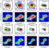 |
Fig. 5 CH3OH zeroth-moment map and pv-diagrams for the transitions listed in Table 1. The top row shows the zeroth-moment map calculated over a velocity range of [−55, −30] km s−1; contours start at 30% of the peak and increase by 15%. The white cross marks the position of the continuum peak. The beam is shown in the lower left corner. The symmetry of the methanol molecule is labelled ineach panel, as well as the upper level energy of the transition. The subsequent row shows the pv-diagram along the Δα axis and averaged over the extent of the cube, corresponding to ~2.5′′. The right-ascension offset of the continuum peak and the vlsr velocity of the source are marked with a white dotted line. Dashed lines show vlsr ± 4.5 km s−1, corresponding to the peak velocity of the CH3OH spots. |
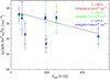 |
Fig. 6 Rotational diagram of the CH3OH (and isotopologue) transitions from Table 1. The colours correspond to the measurements on different positions: green shows the position marked A, red shows the position marked B, and blue corresponds to the central position marked by a cross in Fig. 4. The filled circles show the CH3 OH lines, squares represent the 13CH3OH lines, and triangles show the optically thick lines that are not used for the fit. The error bars show the linearly propagated errors from the Gaussian fit to the integrated intensities. |
3.3.2 LTE modelling with WEEDs
Our observations cover a 7.5 GHz bandwidth, and the spectra extracted towards the CH3OH peak positions show line forests of other molecular species, typically COMs. To analyse the CH3OH emission, wetherefore modelled the entire spectrum using the WEEDs package (Maret et al. 2011) and assumed LTE conditions, which are likely to apply because of the high volume densities. The molecular composition of the gas towards the CH3OH peaks will be described in a forthcoming paper, together with a detailed analysis.
In short, we performed the modelling in an iterative process, and started with the CH3OH lines. The input parameters were the molecular column density, kinetic temperature, source size, vlsr, and line width. Based on these parameters, we fixed the source size to 0.4′′, which means that the emission is resolved, as suggested by the data (Fig. 5). The modelled transitions may have different source sizes, but as long as they are resolved by our observations, the actual source size does not influence the result. The line width of the CH3OH line was obtained by the Gaussian fits to the extracted spectra. After obtaining a first reasonably good fit to the listed CH3OH transitions, we started to subsequently add other molecular species, mainly COMs, which are responsible for the lower intensity lines (Csengeri et al., in prep., b).
We created a grid of models for the CH3OH column density, N(CH3OH), between 1017 and 1020 cm−2, and kinetic temperatures between 50 and 300 K. We sampled the two parameter ranges by 25 linearly spaced values and then visually assessed the results. These models show that the detection or non-detection of certain transitions allows us to place a rather strict upper limit on the kinetic temperature. Above Tkin > 200 K, our models predict that other transitions of the vt = 1 state should be detectable at these column densities; the brightest are at 334.627 GHz (J = 223,0,1−222,0,1), and 334.680 GHz (J = 25−3,0,1−24−2,0,1). Although these frequency ranges are affected by blending with COMs, models with Tkin > 200 K predict that these rotational transitions within its vt = 1 state are brighter than the observed features in the spectrum at their frequency.
Our results give column densities of about 1.2–2 × 1019 cm−2 and a kinetic temperature of about 160–200 K for the two positions. We find that the peak brightness temperatures for the transitions observed across the band are more sensitive to the methanol column density than to the variation in kinetic temperature. While this modelling takes into account blending with other transitions, our results are consistent with the estimates of column density and rotational temperature obtained from the rotational diagram analysis (Sect. 3.3.1).
3.4 Protostellar activity
3.4.1 Outflowing gas traced by the CO (J = 3–2) line
The protostellar activity of the compact continuum source is revealed by a single bipolar molecular outflow shown in Fig. 7. The CO (3–2) line shows emission over a broad velocity range, Δ v, of ±50 km s−1 with respect to the source rest velocity (vlsr) (Fig. 7a). Imaging the highest velocities of this gas reveals a single and collimated bipolar molecular outflow. The orientation of the high-velocity CO emission clearly outlines the axis of material ejection. The high-velocity CO (3–2) emission coincides well with the integrated emission from the shock tracer SiO (8–7) (Fig. 7b), which likely traces the bow shocks along the outflow axis (Fig. 7c).
In particular, the brightest CO emission of the red-shifted northern lobe appears to be confined and terminates within the observed region (Fig. 7c). At the same place as the terminal position of the northern lobe, we detect emission at the source rest velocity of the shocked gas tracer, SiO (8–7), an analogy to the bow shocks observed in the vicinity of low-mass protostars. These indicate that the shock front of the outflowing gas impacts the ambient medium.
When we assume that the maximum velocity observed in the CO (3–2) line corresponds to the speed at which the material has been ejected from the vicinity of the protostar, we can estimate the time at which this material has been ejected. We measure an angular separation of ~10′′ between the central object and the bow shock seen in the SiO (8–7) line, which corresponds to a projected physical distance of 25 000 au.Based on the observed line wings of the CO (3–2) line, the measured velocity extent of the flow is ~50 km s−1. We estimatean inclination angle, i, of 56°, where i = 0° describes a face-on geometry, and i = 90° corresponds to an edge-on view. This is obtained from the axis ratio of the measured envelope size from the dust emission, assuming that it has a circular morphology5. After correcting for the projection effects, we obtain a dynamical age estimate of tdyn ~ 3.5 × 10³ yr for the protostar. This estimate is affected by the uncertainty of the inclination angle, however, and by that of the jet velocity that creates the bow shocks compared to the high-velocity entrained gas seen by CO. While the jet velocity could be higher than traced by the entrained CO emitting gas, which would lead to an even shorter timescale, the highest velocities seen in CO may not reflect the expansion speeds of the outflow lobes as material accelerates. Considering the mass of the central object (Sect. 4.1) and the typically observed infall rates of the order of 10−3 M⊙ yr−1 (Wyrowski et al. 2012, 2016), the higher values of the age estimate, of the order of a few times 103 –104 yr, seem most plausible. This estimate, at the order of magnitude, supports the picture that the protostar is very young.
 |
Fig. 7 Panel a: Colour scale showing the continuum emission from Fig. 1, panel b. The contours show the CO (3–2) integrated emission between − 80 and − 65 km s−1 for the blue, and between − 30 and + 36 km s−1 for the red, respectively. The white cross marks the position of the dust continuum peak. The inset shows a spectrum of the integrated emission over the area of the lowest contours. Panel b: the contours show the velocity-integrated SiO (8–7) emission starting from 4σ (1σ = 0.26 Jy beam−1 km s−1), and increase by 2σ levels. Panel c: overlay of the CO (3–2) contours on the velocity-integrated SiO (8–7) emission shown in panel b. The beam is shown in the lower left corner of each panel. In panel c, it corresponds to that of the CO (3–2) map. |
 |
Fig. 8 Zoom on the envelope showing the CO (3–2) outflow lobes indicated with blue and red contours, the CH3 OH vt = 1 line with black contours. The background shows the dust continuum, and moment-zero maps calculated over a velocity range of − 55 to − 35 km s−1 of SO2, HC3 N (J = 37–36), and HC3N v7 = 1 (J = 38–37) from left to right panels, respectively. The white cross marks the position of the dust continuum peak. The beam of the CO (J = 3–2) datais shown in the lower left corner. |
3.4.2 Sulphur dioxide and cyanoacetylene
To understand the origin of the CH3OH vt = 1 line, we compared its distribution to other species, such as SO2 and cyanoacetylene, HC3N, in Fig. 8. Transitions from the latter species are detected both from the vibrational ground and excited states. These lines are not affected by blending and probe various excitation conditions (see Table 1). It is clear that based on the molecules we studied, the methanol emission corresponds best to the distribution of the dust continuum; both SO2 and HC3N show a different morphology.
We show the SO2 (82,6–71,7) line at 334.673 GHz, which peaks at the position of the protostar and shows the most extended emission of the species discussed here, with a north south elongation that spatially coincides with the outflow axis. Similarly, the HC3N lines peak at the position of the protostar. The v7 = 0 (J = 37–36) transition shows a north–south elongation following the outflow axis and is more compact than the SO2 line. The higher excitation state v7 = 1 (J = 38–37) transition also shows a north–south elongation along the outflow, however, it is even more compact than the vibrational ground-state line.
In Fig. 9, we show horizontal and vertical averages of the datacubes as a function of velocity (pv-diagrams). Owing to the relatively simple source geometry, we show the averages along the Δ α and Δ δ axes. For the CO emission, we use the cube covering the primary beam, while for the other species, we only use the region shown in Fig. 8. The high-velocity outflowing gas is clearly visible in the CO (3–2) line, and the kinematic pattern of both the SO2, and HC3N v7 = 0 lines confirms that they show emission associated with the outflowing molecular gas. The velocity range of the HC3N v7 = 1 emission is clearly broader than that of the CH3OH lines; it is not as broad as the SO2 and HC3N v7 = 0 emission, however. The emission around vlsr ~−33 km s−1 close to the HC3N v7 = 1 line constitutes contamination from COMs with line forests, such as acetone and ethylene glycol.
 |
Fig. 9 pv-diagrams along the Δδ axis and averaged over the extent of the cube (top row) and along the Δ α axis (bottom row) of the CO (3–2), SO2, HC3 N (J = 37–36), and HC3N v7 = 1 (J = 38–37) transitions from left to right panels, respectively. The dotted lines show the vlsr of the source and the position of the dust continuum peak. The dashed lines indicate velocities of vlsr ± 4.5 km s−1, roughly corresponding to the velocities of the CH3OH peaks. The red rectangle in the lower left panel corresponds to the region shown in the other panels. The contours start at 20% of the peak and increase by 10%, except for the panel of the CO and SO2 lines, where the lowest contours start at 5% of the peak. |
4 Discussion
We identifya single high-mass protostellar envelope within the ~600 M⊙ mid-infrared quiet clump, G328.2551–0.5321. In Sect. 4.1 we argue that the protostar is still in its main accretion phase, which resembles the Class 0 phase of low-mass protostars (cf. Duarte-Cabral et al. 2013). We investigate the origin of the CH3OH emission in Sect. 4.2 and propose that in particular the torsionally excited state line traces shocks that are due to the infall from the envelope onto an accretion disc. In Sect. 4.3, we compare its kinematics with a vibrationally excited state transition of HC3N, which we propose as a potential new tracer for the accretion disc.
4.1 Mostmassive envelope of a young protostar
A luminosity of Lbol = 1.3 × 10⁴ L⊙ (see Appendix A) associated with a massive envelope and a strong outflow point to a still strongly accreting, young massive protostar. Owing to the high extinction towards the protostar, we use evolutionary diagrams (Fig. 10) based on protostellar evolution models (Hosokawa & Omukai 2009) to estimate the mass of the central object.
According to models of protostellar evolution, the observed luminosity is too high to originate from accretion alone (Hosokawa et al. 2010), instead, it is rather dominated by the Kelvin–Helmholtz gravitational contraction of the protostellar core. When the typical accretion rate observed towards high-mass protostars and YSOs is used, which is of the order of 10−3 M⊙ yr−1 (Wyrowski et al. 2016), the Hosokawa tracks indicate that the protostar has to be bloated and close to the maximum of its radius during its protostellar evolution, suggesting that it is at the onset of the Kelvin–Helmholtz contraction phase (Hosokawa et al. 2010). In this regime, the luminosity does not depend strongly on the actual accretion rate and mainly depends on the mass of the protostar.
Using these models for the typically expected accretion rate of Ṁacc = 10−3 M⊙ yr−1, we find a central mass of about 11 M⊙ for Lbol = 1.3 × 10⁴ L⊙. Evolutionary tracks with accretion rates of Ṁacc = 1−30 × 10−4 M⊙ yr−1 give a similar protostellar mass range, between 11.1 and 15.2 M⊙, respectively. The protostellar radius adjusts, roughly in a proportional way, to the average accretion rate with a range of radius from 8 to 260 R⊙ for Ṁacc = 1−30 × 10−4 M⊙ yr−1. We can therefore assume that the current protostellar mass is relatively well determined and lies in the range between 11 and 16 M⊙. Taking the dynamical age estimate from Sect. 3.4.1 and the current propostellar mass, we can place an upper limit on the accretion rate through Ṁacc = Mproto∕τdyn, which is between 3.1 × 10⁻³ and 4.2 × 10⁻³ M⊙ yr−1. This estimate is considerably affected by the uncertainties in the dynamical age estimate, however (see Sect. 3.4.1).
Several types of maser emission also support the presence of an already high-mass protostellar object; the evolutionary models indicate, however, that because the protostar is bloated, no strong ionising emission is expected, despite its high mass. This is consistent with the lack of radio continuum detection towards this object and with the fact that it has been identified as a massive YSO in the Red MSX Sources (RMS) survey (Lumsden et al. 2013). The field has been covered at 3.6 and 6 cm by a radio survey of southern RMS (Urquhart et al. 2007) that targeted a nearby MYSO/UC H II region, which only showed radio emission 1.1′ offset compared to our position. Similarly, radio continuum observations at 8.4 GHz only report a 4σ upper limit of 0.6 mJy (Phillips et al. 1998). Based on this upper limit and adopting a spherical model of ionised plasma with typical values of Te = 104 K electron temperature, EM = 108 −1010 pc cm−6 emission measure, we find that only a very compact H II region with a radius of 100 au could have remained undetected in these observations. This is an independent confirmation of the young age of the protostar.
Based on the estimated current core mass of 120 M⊙, we may expect a final stellar mass of ~50 M⊙ (Fig. 10). The protostar of G328.2551–0.5321 is therefore a particularly interesting object, and we suggest that it is a rare example of a bloated, high-mass protostar, precursor of a potentially O4-type to O5-type star. Only very few candidates of such bloated protostars have been reported (e.g. Palau et al. 2013, and references therein), and most of them correspond to objects detected in the optical, and the source presented here is much more embedded.
Throughout this work, we refer to the continuum peak as a single high-mass protostellar envelope. However, we cannot exclude that the source might be fragmented at smaller scales, that is, <400 au, which wouldlead to the formation of a close binary from a single collapsing envelope. While O-type stars have a high multiplicity (e.g. Sana 2017), we do not find clear evidence at the observed scales that would indicate multiplicity on smaller scales. For example, the small outflow opening angle might either suggest that the system is still young or that a single source drives the outflowing gas, or both. Alternatively, gravitational fragmentation of the massive inner envelope could lead to the formation of companions at a subsequent evolutionary stage.
 |
Fig. 10 Evolutionary diagram showing Menv vs. Lbol. The colour scale shows the predicted distribution of protostars as a fraction relative to 1 when the typical stellar initial mass function is accounted for Kroupa & Weidner (2003) and for a star formation and accretion history (constant star formation and decreasing accretion rates) as described in Duarte-Cabral et al. (2013; figure adapted from Motte et al. 2018). The protostar of G328.2551–0.5321 is shown as a filled magenta circle. |
4.2 Accretion shocks at the inner envelope
All CH3OH lines follow the extension of the envelope, and their pv-diagrams are consistent with rotational motions (Fig. 5). Figure 11 shows the contours of the CH3OH vt = 1 line in different velocity channels and reveals a clear velocity gradient over the bulk of the envelope. The most extreme velocity channels show that the emission follows the azimuthal elongations of the envelope well. This gradient is spatially resolved over the blue lobe, which moves in our direction and connects the envelope to the compact dust component. The receding arm, located at the near side of the envelope, is more compact. This is consistent with a picture of spiral streams developing in the collapsing envelope as the material undergoes infall in a flattened geometry. The development of such spirals is frequently seen in numerical simulations of accretion onto a central, dominant protostar. They are typically associated with a flattened structure (e.g. Krumholz et al. 2007; Hennebelle & Ciardi 2009; Kuiper et al. 2011; Hennebelle et al. 2016b). A similar pattern has been observed towards the low-mass sources BHB07-11, in the B59 core (Alves et al. 2017), and Elias 2-27 (Pérez et al. 2016), and also on somewhat larger scales of infalling envelopes towards more evolved high-mass star-forming regions with a luminosity higher by an order of magnitude (Liu et al. 2015).
The peak of the torsionally excited state line, together with the 13C isotopologue lines, pinpoints the location of the highest methanol column densities. We explain these observations by two physical components for the CH3OH emission, the more extended emission associated with the bulk of the inner envelope, and the peak of the vt = 1 line observed at the largest velocity shift compared to the source vlsr. In the following we investigate the physical origin of the vt = 1 emission peaks.
Our LTE analysis suggests a high CH3OH column density up to 2 × 1019 cm−2 towards these positions, which is at least three orders of magnitude higher than typically observed in the quiescent gas (e.g. Bachiller et al. 1995; Liechti & Walmsley 1997). Such high CH3OH column densities are, however, observed on small scales towards high-mass star-forming sites, as reported, for instance, by Palau et al. (2017) in the disc component of a high-mass protostar, IRAS 20126+4104, and towards other high-mass star-forming regions (Beltrán et al. 2014). Towards the hot cores in the most extreme star-forming region, Sgr B2, even higher values are reported above 1019 cm−2 (Bonfand et al. 2017).
In particular, the torsionally excited vt = 1 line with an upper energy level of 315 K typically requires an infrared radiation field at 20–50 μm in order to populate its upper state. Despite the high average volume densities, which are assumed to be above n >107 cm−3, radiative excitation could be necessary to populate rotational levels in the vt = 1 state. Heated dust in the vicinity of the protostar would naturally provide the infrared photons, therefore, it is very surprising that this line does not peak on the dust continuum at the position of the protostar, but instead peaks on the inner envelope (Fig. 4). This particular pattern could be explained by a decrease in CH3OH abundance towards the protostar, and our results in Sect. 3.3.1 indeed suggest somewhat higher CH3OH column densities offset from the dust peak. Considering that the H2 column density increases towards the continuum peak, and since in Sect. 3.2.2, we rule out optical depth effects of the discussed transitions, this suggests a decreasing CH3OH abundance towards the position of the protostar. The observed high CH3OH column densities and their emission peak could also pinpoint local heating from shocks, which would naturally lead to an increase in both the temperature and the molecular abundance, especially for CH3OH. This is because CH3OH has been found to show an increase in abundance by orders of magnitude in various shock conditions as the molecule is released from the grain surfaces via sputtering (Flower et al. 2010; Flower & Pineau des Forêts 2012).
Shocks are produced in a discontinuity in the motion of the gas, and in a collapsing envelope, they can emerge in various conditions. One possibility is an origin associated with the outflowing gas hitting the ambient medium of the envelope. Such an increase in the CH3OH abundance has been observed in both low-mass (Bachiller et al. 1995) and high-mass star-forming regions (Liechti & Walmsley 1997; Palau et al. 2017). We therefore compare the kinematics of the CH3OH emission in more detail with that of outflow tracers in Fig. 12 (see Sect. 3.4.2) to exclude its association with outflow shocks. While the CO (3–2) emission is not useful for velocities below vlsr ± 6 km s−1 because of strong self absorption, the HC3N v7 = 0 line shows a velocity gradient starting at a position close to the protostar and shows increasing velocities at larger distances. The ±4.5 km s−1 peaks of the CH3OH vt = 1 line are offset from the HC3N v7 = 0 transition, showing no evidence for the CH3OH emission to follow the high-velocity emission from the outflowing gas.
Interestingly, a comparison with the HC3N v7 = 1 line (Fig. 12, right panel) shows that the higher excitation gas is more compact and is clearly confined between the spatial and velocity axes that are outlined by CH3OH. The velocity gradient across the line is visible, but its peak is offset from the CH3OH peaks. This supports a picture where the CH3OH and HC3N trace different components, the former tracing the inner envelope more, while the HC3N v7 = 1 line probes the regions closer to the protostar.
Another possibility to explain the methanol peaks would be the launching of the outflow, which would also lead to shocks liberating CH3OH into the gas phase. The launching mechanism of the outflowing gas is highly unexplored territory in high-mass star formation; the location of the outflow launching site is therefore not constrained. Towards low-mass protostars, methanol has been observed to be associated with the launching of the jet/disc wind in the close vicinity, within < 135 au distance from the protostar (Leurini et al. 2016), which is a considerably smaller scale than probed by our observations. There is some indication that towards low-mass protostars, outflow can be launched at the outer regions of the Keplerian accretion disc. A recent study of a low-mass Class I type protostar presents an example where the outflow is launched at a distance beyond the disc edge from the inner envelope (Alves et al. 2017). With our current angular resolution, we do not probe such small scales, which would be unresolved and peak at the location of the protostar. However, we cannot exclude that the observed CH3OH spots may receive contribution from the surface of the flattened envelope.
Given the extent of the torsionally excited CH3OH emission, the best explanation for our observations is that a significant amount of CH3OH is liberated into the gas phase by shocks associated with the inner envelope itself. Around the low-mass Class 0 protostar L1157, CH3OH has been detected to trace shocks within the infalling gas (Goldsmith et al. 1999; Velusamy et al. 2002). In both of the latter two scenarios that explain the CH3OH emission, the observed maximum velocity offset corresponds to the line-of-sight rotational velocity of the gas at the innermost regions of the envelope.
 |
Fig. 11 Panel a: same colour scale as in Fig. 2c, showing the thermal dust emission without the larger scale core emission in order to enhance the structure of the inner envelope. The colour lines show the 50% contour of the peak emission of vt = 1 CH3 OH line at different velocities, starting from − 50.5 km s−1 (blue) to − 38 km s−1 (red). The corresponding velocity of every second contour is shown in the figure legend. Panel b: same as the left panel, but showing the90% contours of the most extreme velocity components in red and blue. The velocities corresponding to each contour are shown in the figure legend. |
 |
Fig. 12 Comparison of the position velocity map along the Δα axis and averaged over a region of ~2.5′′. The colour scale shows the CO (3–2) emission, which is heavily affected by missing spacings and self-absorption at the source vlsr. The dark grey contours show the CH3OH vt = 1, white contours show HC3N (37–37) (left panel) and HC3N v7 = 1 (right panel) transitions. |
4.3 Indirect evidence for a Keplerian disc
The brightest spots of the torsionally excited methanol emission can be interpreted as tracing shocks emerging in the innermost regions of the envelope, and they are therefore associated with the centrifugal barrier. This occurs when the inflowing material from the envelope hits material with a smaller radial velocity component that corresponds to an accretion disc surrounding the central protostar. This transition between the envelope and the disc material at the centrifugal barrier has been directly observed in nearby low-mass protostars (Sakai et al. 2014; Oya et al. 2016; Alves et al. 2017). Towards these objects, the gas kinematics and the gas chemistry both change in the inner envelope; some studies interpret the extent of this region as a sharp (cf. Alves et al. 2017), while others describe it as a more gradual transition region (Oya et al. 2016). Here we observe it as a more extended emission, which also appears to be asymmetric.
Direct evidence for the presence of the disc is limited by the angular and spectral resolution of our dataset; however, by adding all pieces of evidence, we find several indications supporting the scenario of accretion shocks at the centrifugal barrier. In Sect. 3.1, we have noted a marginally resolved, compact dust component that could correspond to the disc with a resolved major axis of 250 au seen in projection. The elongation of this residual is resolved and lies perpendicular to the outflow axis within ~10°. Its orientation and extent are consistent with the location of the two CH3OH peaks at a projected distance of 300–800 au, considering the uncertainty resulting from our angular resolution of ~400 au.
In addition, we find that the highest excitation molecular emission observed by us in the vibrationally excited HC3N v7 = 1 line is very compact and peaks on the compact dust component. This transition has an upper level energy of 645 K and also requires an infrared radiation field at 20–50 μm in order to populate its vibrationally excited states. Therefore, it more likely traces a region that is considerably closer to the protostar than the torsionally excited methanol line. Although this molecule is also present in the outflow, as suggested by the vibrational ground-state transition, we propose that the high-excitation vibrationally excited HC3N v7 = 1 emission is a good candidate for tracing emission from the accretion disc.
Because the accretion disc is expected to be in Keplerian rotation, we can compare the observed pv-diagrams with a simple toy model adapted from Ohashi et al. (1997) to describe an axisymmetric rotating thin disc for the HC3N v7 = 1 line and a ring of gas at the centrifugal barrier for the CH3OH vt = 1 line (Fig. 13). We show two models here: the CH3OH lines trace the rotating envelope with vrot(r) ~ r−1, and the HC3N v7 = 1 line traces the gas in Keplerian motion.
We used an x,y grid size of 2 × 2500 au, and a velocity axis with 0.7 km s−1 resolution, a power-law density distribution with n ∝ r−1.5, constant molecular abundance with respect to H2, and a central protostellar mass of 15 M⊙ (see Sect. 4.1). For the geometry of the CH3OH emission, weused a ring between 300 and 900 au, corresponding to the extent of the marginally resolved compact component, and vrot = 4.5 km s−1 at the inner radius of 300 au. For the HC3N v7 = 1 line, we used a Keplerian model with a disc size of up to 600 au.
The models are shown in Fig. 13 for the ring (top row) and the disc (bottom row) component. The observed spots of CH3OH that correspond to the highest column densities are reasonably well reproduced with these models. The observed asymmetries in the distribution of the emission and projection effects are not included in our models, however. We break the degeneracy between the location of the ring of CH3OH emitting gas and the mass of the central object by measuring the position of the methanol shocks. Since we do not include a correction for the inclination angle between the source and our line of sight, the determined parameters are uncertain within a factor of a few.
These models demonstrate that the CH3OH emission can be well explained by a ring of emitting gas from the infalling envelope that is more extended than the observed HC3N v7 = 1 line, and by the compact dust continuum source. This scenario is similar to what has been observed towards the high-mass object AFGL2591 by Jiménez-Serra et al. (2012), who find a ring of CH3OH emission at a velocity that is consistent with the Keplerian velocity of the estimated source mass of 40 M⊙. Because of the observed asymmetry of the HC3N v7 = 1 line and our poor velocity resolution, our models only show that the extent of the observed velocity range of the HC3N v7 = 1 line could be consistent with a disc in Keplerian rotation based on the physical constraints of the model.
Finally, in Fig. 14, we show analytic estimates for the Keplerian velocity at a range of central mass between 10 and 20 M⊙, and a range of centrifugal barriers around 300–800 au, which corresponds to the parameter range that could still be consistent with the observations. To obtain the rotational velocity at this radius, we corrected the observed 4.5 km s−1 for an inclination angle, i, of 56° based on the axis ratio of the measured envelope size in Sect. 3.1. The observed velocity offset of the CH3OH peaks fits the Keplerian velocity well for the plausible mass range and the range of the centrifugal barrier within a resolution element.
 |
Fig. 13 Left column: pv-diagram of models with a rotating ring with vr ~ r (top panel), and with a disc in Keplerian rotation (bottom panel). Right column: colour scale showing the zeroth-moment maps for the 334.42 GHz CH3OH vt = 1 line (top panel) and the 346.456 GHz HC3N v7 = 1 line (bottom panel). Contours are the same as in the left column and show the model prediction. |
4.4 Physical properties of discs around high-mass protostars
Although massive rotating toroids towards precursors of OB-type stars have been frequently detected (Beltrán et al. 2004, 2014; Sánchez-Monge et al. 2013; Cesaroni et al. 2014, 2017), clear signatures of accretion discs around high-mass protostars are still challenging to identify, in particular towards the precursors of the most massive O-type stars (Beltrán & de Wit 2016). Our results suggest the presence of an accretion disc around a still deeply embedded young high-mass protostar that is likely to be a precursor of an O4-O5 type star. Our findings suggest that a disc may have formed already at this early stage, providing observational support to numerical simulations, which predict that despite the strong radiation pressure exerted by high-mass protostars, accretion through flattened structures and discs enable the formation of the highest mass stars (Krumholz et al. 2009; Kuiper et al. 2010, 2011).
Together with other examples of envelope-outflow-disc systems (e.g. Johnston et al. 2015; Beltrán & de Wit 2016), this suggests a physical picture of high-mass star formation on a core scale that is qualitatively very similar to that of low-mass objects. As observed towards L1527 (Sakai et al. 2014), TMC-1 (Aso et al. 2015), and VLA1623A (Murillo et al. 2013), we also see evidence for shocks induced by the infall from the envelope to the disc that impose a change in the chemical composition of the infalling gas at the centrifugal barrier (see also Oya et al. 2017). The accretion disc around the protostar of L1527 has been confirmed since then with direct imaging (Sakai et al. 2017).
Our findings suggest considerably different physical conditions and chemical environment for high-mass protostars, however. The observed prominent CH3OH emission peak that we explain by shocks at the centrifugal barrier blends with the more diffuse emission from the envelope. At our spatial resolution, these shocks do not outline a sharp boundary, and leave us with a relatively large range of disc radii that are still consistent with the observations. Based on the size of the compact dust continuum source, we measure a minimum projected radius of ~250 au for the disc major axis, while the maximum outer radius, constrained by the peak of the CH3OH emission, is located somewhere between 300 and 800 au. Correcting these values for an orientation angle of ϕ ~ 12° based on the fitted position angle of the dust residual emission results in a disc radius between 255 and 817 au, which is a factor of few larger than recent ALMA observations suggest for discs around some low-mass Class 0 protostars (e.g. Oya et al. 2016; Sakai et al. 2017). For the rotational velocity at this outer radius, we take the velocity offset of the CH3OH peaks corrected for the inclination angle (Sect. 4.2). Taking an average disc size between the minimum and maximum expected values implies that the local specific angular momentum j∕m = R × vrot = 4.5 × 1021 cm2 s−1, where R is the disc radius and vrot is the rotational velocity of the disc at the given radius.
In Fig. 15, we compare our measurement to values from the literature following Ohashi et al. (1997) and Belloche et al. (2002), and complement it with high-mass discs and toroids from Beltrán & de Wit (2016). We recognise that the local specific angular momentum is considerably higher for the high-mass objects than for the low-mass objects, although the disc candidates observed so far are still at larger physical scales, and they typically lie towards objects that are likely in a more evolved stage than the protostar of G328.2551–0.5321. This suggests that the kinetic energy may be higher at the onset of the collapse in the case of high-mass star formation. The higher kinetic energy could be explained if the collapse sets in at the clump scale, that is, at >0.3 pc scales, compared to the core-scale collapse that is typical for the formation of low-mass protostars. The high specific angular momentum towards high-mass protostars is, therefore, in agreement with the scenario of global collapse or models based on cloud–cloud collisions at the origin of high-mass stars.
A dust-based mass estimate for the disc is very uncertain, not only due to the uncertainty of the temperature, but also because of the unknown dust opacity. Assuming the same dust parameters as for the envelope and taking Tdust = 150 K, we obtain sub-solar mass estimates around Mdisc < 0.25M⊙. Such an elevated temperature is expected for the disc in the close vicinity of the protostellar embryo, but it is still consistent with the SED because of the high optical depth of the cooler dust. Since our disc mass estimate is sub-solar, it is likely that the disc mass is below 10% of the mass of the central object and thus gravitationally stable. Whether the disc itself is stable is an important question; unstable massive discs could either lead to episodic accretion bursts, or undergo fragmentation (Vorobyov & Basu 2010). Both phenomena are observed towards low-mass protostars (the FU Ori phenomen); in particular, multiplicity within low-mass cores has recently been explained by disc fragmentation (Tobin et al. 2016). On the other hand, the high-mass disc candidate AFGL 4176 (Johnston et al. 2015) is more extended, but also more massive. Fragmentation of massive or unstable discs and toroids around high-mass stars could explain why short-period binaries have the highest frequency among O-type stars (Sana 2017).
 |
Fig. 14 Keplerian velocity as a function of radius, r, from the central object for 10, 15, and 20 M⊙. The projection corrected velocity determined from the 334.42 GHz CH3OH vt = 1 line is marked as a grey horizontal line. The grey shaded area corresponds to the projected distance range for the position of the CH3OH vt = 1 spots. |
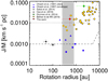 |
Fig. 15 Local specific angular momentum (j∕m = R × vrot) as a function of radius for a sample of low- and high-mass protostars and YSOs. The high-mass sample (Guzmán et al. 2014; Beltrán & de Wit 2016) corresponds to high-mass YSOs with disc candidates, the low-mass objects (Ohashi et al. 1997; Sakai et al. 2014; Oya et al. 2016) correspond to envelopes and discs identified around low-mass Class 0 protostars. Where no explicit information was available, we adopt a 50% uncertainty for the rotation radius, and a linearly propagated 50% uncertainty on the estimated specific angular momentum. For our target, we estimate a 52% uncertainty on these values based on the uncertainty in the disc radius estimate. In this plot, we made no attempt to correct for the source inclination angle. The dashed line shows the j = 0.001 km s−1 line (Belloche 2013) and an angular velocity Ω = 1.8 km s−1 pc−1. For the high-mass sample, we show the j = 0.01 km s−1 pc−1 line and Ω = 50 km s−1 pc−1. The grey shaded area shows our range of disc size estimates. |
4.5 Implications for high-mass star formation
We simultaneously observe a massive core that is not fragmented down to our resolution limit of ~400 au, and find strong evidence for a centrifugal barrier at a large radius of 300–800 au. This may appear contradictory and needs to be discussed. The observed indication for the Keplerian disc together with the high angular momentum suggests that magnetic braking has not been efficient in evacuating and redistributing the angular momentum. Numerical simulations predict that in particular in the early phase of the collapse, the angular momentum from the accretion disc can be efficiently removed through magnetic braking, and can thereby suppress the formation of large discs (e.g. Seifried et al. 2011; Myers et al. 2013; Hennebelle et al. 2016a). Our observations therefore point to a relatively weak magnetic field. On the other hand, despite its high mass, which is two orders of magnitude higher than the thermal Jeans mass, the core did not fragment and appears to be collapsing monolithically, which is consistent with the turbulent core model (McKee & Tan 2003). This would require additional support to complement the thermal pressure, which can be either magnetic or turbulent. Neither the line widths nor the high angular momentum are consistent with strong enough turbulence or magnetic fields, therefore the properties of the core embedded in G328.2551–0.5321 appear difficult to explain.
However, if turbulence or strong ordered motions are present, the misalignment between the magnetic field lines and the angular momentum vectors can limit the effect of magnetic braking, leading to a less efficient removal of the angular momentum (Myers et al. 2013). Alternatively, the present-day properties of the collapsing core and the physical state of the pre-stellar core prior to collapse may have been significantly different at the onset of the collapse. Observations of the small-scale properties of high-mass protostars and the physical properties of their accretion disc, such as in G328.2551–0.5321, may thus challenge high-mass star formation theories. Clearly, more observational examples of accretion discs around high-mass protostars are needed to place further constrains on the formation and properties of discs, and on the collapse scenario.
5 Summary and conclusions
We presented a case study of one of the targets from the SPARKS project, which uses high angular-resolution ALMA observations to study the sample of the most massive mid-infrared quiet massive clumps selected from the ATLASGAL survey. Our observations reveal a single massive protostellar envelope associated with the massive clump, G328.2551–0.5321. Based on protostellar evolutionary tracks, we estimate the current protostellar mass to be between 11 and 16 M⊙, surrounded by a massive core of ~120 M⊙. The estimated envelope mass is an order of magnitude higher than the currently estimated protostellar mass, making this object an excellent example of a high-mass protostar in its main accretion phase, similar to the low-mass Class 0 phase.
We discovered torsionally excited CH3OH spots offset from the protostar with a velocity offset of ±4.5 km s−1 compared to the source vlsr. These peaks are best explained by shocks from the infalling envelope onto the centrifugal barrier. Based on the observed unblended methanol transitions, we estimate the physical conditions on these spots, and find Tkin = 160−170 K, and N(CH3OH) = 1.2−2 × 1019 cm−2, suggesting high CH3OH column densities.
Our analysis of the dust emission reveals azimuthal elongations associated with the dust continuum peak, and a compact component with a marginally resolved beam-deconvolved R90% radius of ~250 au measured along is major axis. This component is consistent with an accretion disc within the centrifugal barrier outlined by the CH3OH shock spots at a distance between ~300 and 800 au offset from the protostar. Furthermore, we propose the vibrationally excited HC3N from energy levels >500 K above ground as potential new tracers for the emission from the accretion disc.
Our results for the first time dissect a clearly massive protostellar envelope potentially forming an O4-O5 type star. The physical picture is qualitatively very similar to that of the low-mass star formation process, but quantitatively, both the physical and the chemical conditions show considerable differences. Our estimate of the specific angular momentum carried by the inner envelope at its transition to an accretion disc is an order of magnitude higher than that observed around low-mass stars. This is consistent with the scenario of global collapse, where the larger collapse scale would naturally lead to a higher angular momentum than in core-collapse models.
Acknowledgements
We thank the referee for the careful reading of the manuscript. This paper makes use of the ALMA data: ADS/JAO.ALMA 2013.1.00960.S. ALMA is a partnership of ESO (representing its member states), NSF (USA), and NINS (Japan), together with NRC (Canada), NSC and ASIAA (Taiwan), and KASI (Republic of Korea), in cooperation with the Republic of Chile. The Joint ALMA Observatory is operated by ESO, AUI/NRAO, and NAOJ. T.Cs. acknowledges support from the Deutsche Forschungsgemeinschaft, DFG via the SPP (priority programme) 1573 “Physics of the ISM”. H.B. acknowledges support from the European Research Council under the Horizon 2020 Framework Program via the ERC Consolidator Grant CSF-648505. L.B. acknowledges support by CONICYT Project PFB06. A.P. acknowledges financial support from UNAM and CONACyT, Mexico.
Appendix A Dust spectral energy distribution and modelling
We constructed the SED of the protostar embedded in the clump G328.2551–0.5321 from the mid-infrared wavelengths up to the radio regime (Fig. A.1) in order to estimate its bolometric luminosity (Lbol), and constrain a representative dust temperature (Td) for the bulk of the mass using a model of greybody emission.
In Fig. A.1, we show the flux densities from the GLIMPSE catalogue at the shortest indicated wavelengths (Benjamin et al. 2003), as well as the WISE band 4 photometry at 22 μm (Cutri et al. 2012). To illustrate the complexity of the region, we show the emission from the far-infrared and millimeter wavelength range in Fig.A.2 using Herschel/Hi-GAL data (Molinari et al. 2010), and the ATLASGAL-Planck combined data at 870 μm (Csengeri et al. 2016). This shows that the emission is largely dominated by extended structures at all these wavelengths.
 |
Fig. A.1 SED of the embedded protostar within the ATLASGAL clump, G328.2551–0.5321. The origin of the flux densities are labelled in the figure legend and are described in the text. The solid line shows the result of a two-component (warm and cold) grebody fit with 48 K and 22 K. The individual components are shown as a dashed grey line. |
 |
Fig. A.2 Far-infrared multi-wavelength view of the ATLASGAL clump, G328.2551–0.5321, using the Herschel Hi-GAL images (Molinari et al. 2016), and the APEX/LABOCA and Planck combined maps (Csengeri et al. 2016). The position of the identified source is marked with a black cross, dotted grey ellipses show the corresponding sources from the Hi-GAL and ATLASGAL catalogues (Csengeri et al. 2014; Molinari et al. 2016, respectively). The solid circle shows half the 8′′ FWHM, corresponding to the scale of the MDC. The FWHM beam widths are shown in the lower left corner of each panel. The colour scale is on a logarithmic scale, and the black line shows the labelled flux density value. |
For comparison, we show the corresponding sources identified in the Herschel/Hi-GAL point source catalogue (Molinari et al. 2016), and the ATLASGAL Gaussclumps source catalogue (Csengeri et al. 2014). The 870 μm flux density measurement by ALMA reveals the MDC at a size-scale of 0.06 pc (see also Csengeri et al. 2017b) and therefore places constraints on the extent of the embedded source. To derive the properties of the gas representative of the embedded protostar, our aim is to extract and scale the flux densities corresponding to a source at ~8 ′′ (the geometric mean of the PACS 70 μm beam; Molinari et al. 2016) with a density profile of n ~ r−2, and neglecting any temperature gradient. To do this, we performed aperture photometry on the PACS 70 μm and 160 μm maps by first measuring the peak intensity at the position of our target within a single beam (taking 5.8′′ × 12.1′′ and 11.4′′× 13.4′′, respectively), and then measured the background emission in three different annuli at increasing distance from 15′′ to 35′′ with respect to the source. For the SPIRE 250, 350, and 500 μm data, we used the values from the Herschel/Hi-GAL point source catalogue and scaled them by adopting the geometric mean of the measured major and minor axes (Molinari et al. 2016).
To obtain the bolometric luminosity of the protostar, we added the entire emission from the near- and mid-infrared to 870 μm, and obtain 1.3 × 10⁴ Lbol. As a comparison, we also calculated the internal luminosity of the protostar using the empirical relation between Lbol and the flux density measured at 70 μm (Dunham et al. 2008), and obtain 1.2 × 10⁴ Lbol. The significant confusion due to extended emission from the mid-infrared to the submillimeter wavelengths adds some uncertainty to our estimate; however, the measured values likely correspond to an upper limit to the luminosity.
To obtain an estimate of the dust temperature, Td, we performed a greybody fit to the far-infrared points of the SED between 70 and 870 μm. Since at 70 μm the emissionis mostly dominated by the heated dust in the vicinity of the protostar, we used a two-component greybody to model the SED, which reveals that the temperature corresponding to the cold gas component dominates the bulk of the emission, and places strong constraints on the warm gas temperature, as well as on the fraction of the heated gas mass. We used κ345 GHz = 0.0185 g cm−2 and an emissivity index of β = 2, where  . We obtain a cold gas component at 22 K, and a warm gas component at 48 K that contains <5% of the total gas mass. The result of the SED fit is shown in Fig. A.1.
References
- Alves, F. O., Girart, J. M., Caselli, P., et al. 2017, A&A, 603, L3 [NASA ADS] [CrossRef] [EDP Sciences] [Google Scholar]
- André, P., Ward-Thompson, D., & Barsony, M. 2000, in Protostars and Planets IV, eds. V. Mannings, A. Boss, & S. S. Russell (University of Arizona Press), 59 [Google Scholar]
- Aso, Y., Ohashi, N., Saigo, K., et al. 2015, ApJ, 812, 27 [NASA ADS] [CrossRef] [Google Scholar]
- Bachiller, R., Liechti, S., Walmsley, C. M., & Colomer, F. 1995, A&A, 295, L51 [NASA ADS] [Google Scholar]
- Belloche, A. 2013, in EAS Pub. Ser., 62, 25 [CrossRef] [EDP Sciences] [Google Scholar]
- Belloche, A., André, P., Despois, D., & Blinder, S. 2002, A&A, 393, 927 [Google Scholar]
- Beltrán, M. T., & de Wit, W. J. 2016, A&ARv, 24, 6 [NASA ADS] [CrossRef] [Google Scholar]
- Beltrán, M. T., Cesaroni, R., Neri, R., et al. 2004, ApJ, 601, L187 [NASA ADS] [CrossRef] [Google Scholar]
- Beltrán, M. T., Cesaroni, R., Neri, R., et al. 2005, A&A, 435, 901 [NASA ADS] [CrossRef] [EDP Sciences] [Google Scholar]
- Beltrán, M. T., Cesaroni, R., Neri, R., & Codella, C. 2011, A&A, 525, A151 [NASA ADS] [CrossRef] [EDP Sciences] [Google Scholar]
- Beltrán, M. T., Sánchez-Monge, Á., Cesaroni, R., et al. 2014, A&A, 571, A52 [NASA ADS] [CrossRef] [EDP Sciences] [Google Scholar]
- Benjamin, R. A., Churchwell, E., Babler, B. L., et al. 2003, PASP, 115, 953 [NASA ADS] [CrossRef] [Google Scholar]
- Beuther, H., Schilke, P., Menten, K. M., et al. 2002, ApJ, 566, 945 [NASA ADS] [CrossRef] [Google Scholar]
- Bonfand, M., Belloche, A., Menten, K. M., Garrod, R. T., & Müller, H. S. P. 2017, A&A, 604, A60 [NASA ADS] [CrossRef] [EDP Sciences] [Google Scholar]
- Bontemps, S., Andre, P., Terebey, S., & Cabrit, S. 1996, A&A, 311, 858 [NASA ADS] [Google Scholar]
- Bontemps, S., Motte, F., Csengeri, T., & Schneider, N. 2010, A&A, 524, A18 [NASA ADS] [CrossRef] [EDP Sciences] [Google Scholar]
- Carey, S. J., Noriega-Crespo, A., Mizuno, D. R., et al. 2009, PASP, 121, 76 [NASA ADS] [CrossRef] [Google Scholar]
- Cesaroni, R., Galli, D., Neri, R., & Walmsley, C. M. 2014, A&A, 566, A73 [NASA ADS] [CrossRef] [EDP Sciences] [Google Scholar]
- Cesaroni, R., Sánchez-Monge, Á., Beltrán, M. T., et al. 2017, A&A, 602, A59 [NASA ADS] [CrossRef] [EDP Sciences] [Google Scholar]
- Csengeri, T., Urquhart, J. S., Schuller, F., et al. 2014, A&A, 565, A75 [NASA ADS] [CrossRef] [EDP Sciences] [Google Scholar]
- Csengeri, T., Leurini, S., Wyrowski, F., et al. 2016, A&A, 586, A149 [NASA ADS] [CrossRef] [EDP Sciences] [Google Scholar]
- Csengeri, T., Bontemps, S., Wyrowski, F., et al. 2017a, A&A, 601, A60 [NASA ADS] [CrossRef] [EDP Sciences] [Google Scholar]
- Csengeri, T., Bontemps, S., Wyrowski, F., et al. 2017b, A&A, 600, L10 [NASA ADS] [CrossRef] [EDP Sciences] [Google Scholar]
- Cutri, R. M., Wright, E. L., Conrow, T., et al. 2012, Explanatory Supplement to the WISE All-Sky Data Release Products, Tech. Rep. [Google Scholar]
- Duarte-Cabral, A., Bontemps, S., Motte, F., et al. 2013, A&A, 558, A125 [NASA ADS] [CrossRef] [EDP Sciences] [Google Scholar]
- Dunham, M. M., Crapsi, A., Evans, II, N. J., et al. 2008, ApJS, 179, 249 [NASA ADS] [CrossRef] [Google Scholar]
- Flower, D. R.,& Pineau des Forêts, G. 2012, MNRAS, 421, 2786 [NASA ADS] [CrossRef] [Google Scholar]
- Flower, D. R., Pineau Des, G., & Rabli, D. 2010, MNRAS, 409, 29 [NASA ADS] [CrossRef] [Google Scholar]
- Garay, G., Mardones, D., Bronfman, L., et al. 2010, ApJ, 710, 567 [NASA ADS] [CrossRef] [Google Scholar]
- Goldsmith, P. F., Langer, W. D., & Velusamy, T. 1999, ApJ, 519, L173 [NASA ADS] [CrossRef] [Google Scholar]
- Gómez, L., Wyrowski, F., Pillai, T., Leurini, S., & Menten, K. M. 2011, A&A, 529, A161 [NASA ADS] [CrossRef] [EDP Sciences] [Google Scholar]
- Guzmán, A. E., Garay, G., & Brooks, K. J. 2010, ApJ, 725, 734 [NASA ADS] [CrossRef] [Google Scholar]
- Guzmán, A. E., Garay, G., Rodríguez, L. F., et al. 2014, ApJ, 796, 117 [NASA ADS] [CrossRef] [Google Scholar]
- Hennebelle, P., & Ciardi, A. 2009, A&A, 506, L29 [NASA ADS] [CrossRef] [EDP Sciences] [Google Scholar]
- Hennebelle, P., Commerçon, B., Chabrier, G., & Marchand, P. 2016a, ApJ, 830, L8 [NASA ADS] [CrossRef] [Google Scholar]
- Hennebelle, P., Lesur, G., & Fromang, S. 2016b, A&A, 590, A22 [NASA ADS] [CrossRef] [EDP Sciences] [Google Scholar]
- Hosokawa, T., & Omukai, K. 2009, ApJ, 691, 823 [NASA ADS] [CrossRef] [Google Scholar]
- Hosokawa, T., Yorke, H. W., & Omukai, K. 2010, ApJ, 721, 478 [NASA ADS] [CrossRef] [Google Scholar]
- Jiménez-Serra, I., Zhang, Q., Viti, S., Martín-Pintado, J., & de Wit, W.-J. 2012, ApJ, 753, 34 [NASA ADS] [CrossRef] [Google Scholar]
- Johnston, K. G., Robitaille, T. P., Beuther, H., et al. 2015, ApJ, 813, L19 [NASA ADS] [CrossRef] [Google Scholar]
- Kroupa, P., & Weidner, C. 2003, ApJ, 598, 1076 [NASA ADS] [CrossRef] [Google Scholar]
- Krumholz, M. R., Klein, R. I., & McKee, C. F. 2007, ApJ, 656, 959 [NASA ADS] [CrossRef] [Google Scholar]
- Krumholz, M. R., Klein, R. I., McKee, C. F., Offner, S. S. R., & Cunningham, A. J. 2009, Science, 323, 754 [NASA ADS] [CrossRef] [PubMed] [Google Scholar]
- Kuiper, R., Klahr, H., Beuther, H., & Henning, T. 2010, ApJ, 722, 1556 [CrossRef] [Google Scholar]
- Kuiper, R., Klahr, H., Beuther, H., & Henning, T. 2011, ApJ, 732, 20 [NASA ADS] [CrossRef] [Google Scholar]
- Langer, W. D., & Penzias, A. A. 1990, ApJ, 357, 477 [NASA ADS] [CrossRef] [Google Scholar]
- Leurini, S., Codella, C., Cabrit, S., et al. 2016, A&A, 595, L4 [NASA ADS] [CrossRef] [EDP Sciences] [Google Scholar]
- Liechti, S., & Walmsley, C. M. 1997, A&A, 321, 625 [NASA ADS] [Google Scholar]
- Liu, H. B., Galván-Madrid, R., Jiménez-Serra, I., et al. 2015, ApJ, 804, 37 [NASA ADS] [CrossRef] [Google Scholar]
- Lumsden, S. L., Hoare, M. G., Urquhart, J. S., et al. 2013, ApJS, 208, 11 [NASA ADS] [CrossRef] [Google Scholar]
- Maret, S., Hily-Blant, P., Pety, J., Bardeau, S., & Reynier, E. 2011, A&A, 526, A47 [NASA ADS] [CrossRef] [EDP Sciences] [Google Scholar]
- McKee, C. F.,& Tan, J. C. 2003, ApJ, 585, 850 [NASA ADS] [CrossRef] [MathSciNet] [Google Scholar]
- Milam, S. N., Savage, C., Brewster, M. A., Ziurys, L. M., & Wyckoff, S. 2005, ApJ, 634, 1126 [NASA ADS] [CrossRef] [Google Scholar]
- Molinari, S., Brand, J., Cesaroni, R., & Palla, F. 2000, A&A, 355, 617 [NASA ADS] [Google Scholar]
- Molinari, S., Swinyard, B., Bally, J., et al. 2010, PASP, 122, 314 [NASA ADS] [CrossRef] [Google Scholar]
- Molinari, S., Schisano, E., Elia, D., et al. 2016, A&A, 591, A149 [NASA ADS] [CrossRef] [EDP Sciences] [Google Scholar]
- Moscadelli, L., Sánchez-Monge, Á., Goddi, C., et al. 2016, A&A, 585, A71 [NASA ADS] [CrossRef] [EDP Sciences] [Google Scholar]
- Motte, F., Bontemps, S., Schilke, P., et al. 2007, A&A, 476, 1243 [NASA ADS] [CrossRef] [EDP Sciences] [Google Scholar]
- Motte, F., Bontemps, S., & Louvet, F. 2018, ARA&A, in press [arXiv:1706.00118] [Google Scholar]
- Mottram, J. C., Hoare, M. G., Urquhart, J. S., et al. 2011, A&A, 525, A149 [NASA ADS] [CrossRef] [EDP Sciences] [Google Scholar]
- Murillo, N. M., Lai, S.-P., Bruderer, S., Harsono, D., & van Dishoeck E. F. 2013, A&A, 560, A103 [NASA ADS] [CrossRef] [EDP Sciences] [Google Scholar]
- Myers, A. T., McKee, C. F., Cunningham, A. J., Klein, R. I., & Krumholz, M. R. 2013, ApJ, 766, 97 [NASA ADS] [CrossRef] [Google Scholar]
- Ohashi, N., Hayashi, M., Ho, P. T. P., & Momose, M. 1997, ApJ, 475, 211 [Google Scholar]
- Ossenkopf, V., & Henning, T. 1994, A&A, 291, 943 [NASA ADS] [Google Scholar]
- Oya, Y., Sakai, N., López-Sepulcre, A., et al. 2016, ApJ, 824, 88 [NASA ADS] [CrossRef] [Google Scholar]
- Oya, Y., Sakai, N., Watanabe, Y., et al. 2017, ApJ, 837, 174 [NASA ADS] [CrossRef] [Google Scholar]
- Palau, A., Fuente, A., Girart, J. M., et al. 2013, ApJ, 762, 120 [NASA ADS] [CrossRef] [Google Scholar]
- Palau, A., Walsh, C., Sánchez-Monge, Á., et al. 2017, MNRAS, 467, 2723 [NASA ADS] [Google Scholar]
- Peretto, N., Fuller, G. A., Duarte-Cabral, A., et al. 2013, A&A, 555, A112 [NASA ADS] [CrossRef] [EDP Sciences] [Google Scholar]
- Pérez, L. M., Carpenter, J. M., Andrews, S. M., et al. 2016, Science, 353, 1519 [NASA ADS] [CrossRef] [Google Scholar]
- Phillips, C. J., Norris, R. P., Ellingsen, S. P., & McCulloch, P. M. 1998, MNRAS, 300, 1131 [NASA ADS] [CrossRef] [Google Scholar]
- Purser, S. J. D., Lumsden, S. L., Hoare, M. G., et al. 2016, MNRAS, 460, 1039 [NASA ADS] [CrossRef] [Google Scholar]
- Rosero, V., Hofner, P., Claussen, M., et al. 2016, ApJS, 227, 25 [NASA ADS] [CrossRef] [Google Scholar]
- Sakai, N., Sakai, T., Hirota, T., et al. 2014, Nature, 507, 78 [NASA ADS] [CrossRef] [Google Scholar]
- Sakai, N., Oya, Y., Higuchi, A. E., et al. 2017, MNRAS, 467, L76 [NASA ADS] [Google Scholar]
- Sana, H. 2017, in The Lives and Death-Throes of Massive Stars, eds. J. J. Eldridge, J. C. Bray, L. A. S. McClelland, & L. Xiao, IAU Symp., 329, 110 [Google Scholar]
- Sánchez-Monge, Á., Cesaroni, R., Beltrán, M. T., et al. 2013, A&A, 552, L10 [NASA ADS] [CrossRef] [EDP Sciences] [Google Scholar]
- Sanna, A., Surcis, G., Moscadelli, L., et al. 2015, A&A, 583, L3 [NASA ADS] [CrossRef] [EDP Sciences] [Google Scholar]
- Schöier, F. L., van der Tak, F. F. S., van Dishoeck, E. F., & Black, J. H. 2005, A&A, 432, 369 [NASA ADS] [CrossRef] [EDP Sciences] [Google Scholar]
- Schuller, F., Menten, K. M., Contreras, Y., et al. 2009, A&A, 504, 415 [NASA ADS] [CrossRef] [EDP Sciences] [Google Scholar]
- Seifried, D., Banerjee, R., Klessen, R. S., Duffin, D., & Pudritz, R. E. 2011, MNRAS, 417, 1054 [NASA ADS] [CrossRef] [Google Scholar]
- Sridharan, T. K., Beuther, H., Schilke, P., Menten, K. M., & Wyrowski, F. 2002, ApJ, 566, 931 [NASA ADS] [CrossRef] [Google Scholar]
- Tanaka, K. E. I., Tan, J. C., & Zhang, Y. 2017, ApJ, 835, 32 [NASA ADS] [CrossRef] [Google Scholar]
- Tobin, J. J., Kratter, K. M., Persson, M. V., et al. 2016, Nature, 538, 483 [NASA ADS] [CrossRef] [Google Scholar]
- Urquhart, J. S., Busfield, A. L., Hoare, M. G., et al. 2007, A&A, 461, 11 [NASA ADS] [CrossRef] [EDP Sciences] [Google Scholar]
- Velusamy, T., Langer, W. D., & Goldsmith, P. F. 2002, ApJ, 565, L43 [NASA ADS] [CrossRef] [Google Scholar]
- Vorobyov, E. I., & Basu, S. 2010, ApJ, 719, 1896 [NASA ADS] [CrossRef] [Google Scholar]
- Wyrowski, F., Güsten, R., Menten, K. M., Wiesemeyer, H., & Klein, B. 2012, A&A, 542, L15 [NASA ADS] [CrossRef] [EDP Sciences] [Google Scholar]
- Wyrowski, F., Güsten, R., Menten, K. M., et al. 2016, A&A, 585, A149 [NASA ADS] [CrossRef] [EDP Sciences] [Google Scholar]
- Zhang, Q., Hunter, T. R., Brand, J., et al. 2005, ApJ, 625, 864 [NASA ADS] [CrossRef] [Google Scholar]
Mid-infrared quiet massive clumps are defined by weak or no emission in the 21−24 μm wavelength range. We follow here the definition of Csengeri et al. (2017a), which is based on Motte et al. (2007). As discussed there, our mid-infrared flux limit corresponds to that of an embedded star with 104 L⊙.
In Csengeri et al. (2017a), we used Td = 25 K for all cores.
We adopt the vlsr of the dense gas in the clump/core scale, as used in Csengeri et al. (2017a).
The CH3 OH − E transitions in the band have Einstein coefficients that are an order of magnitude smaller, which might explain why all the CH3 OH − E lines show two emission peaks despite their lower energy level.
The outflow is rather confined, it has a small opening angle of ~ 30°. Simple geometric considerations based on the outflow orientation, opening angle, and the fact that there is no significant overlap along the line of sight between the blue- and red-shifted emission, mean that we can exclude an inclination angle range between i < 15°, and i > 75°. An inclination angle range between 15° and 75° would result in tdyn = 6.3 × 10²−8.8 × 10³ yr.
All Tables
Observational parameters for the CH3OH vt = 1 lines, and results of the LTE modelling for CH3OH.
All Figures
|
Fig. 1 Overview of the region centred on ℓ = +328.2551, b = −0.5321 in Galactic coordinates. Left panel: the three-colour composite image is from the Spitzer/GLIMPSE (Benjamin et al. 2003) and MIPSGAL (Carey et al. 2009) surveys (blue: 4.5 μm, green: 8 μm, and red: 24 μm) and is shownin Galactic coordinates. The contours show the 870 μm continuum emission from the ATLASGAL survey (Schuller et al. 2009; Csengeri et al. 2014). The arrow marks the dust continuum peak of the targeted clump, and the circle corresponds to the region shown in the right panel. Right panel: line-free continuum emission imaged at 345 GHz with the ALMA 12 m array. The colour scale is linear from − 3σ to 120σ. The contour shows the 7σ level. The FWHM size of the synthesised beam is shown in the lower left corner. |
| In the text | |
|
Fig. 2 Zoom on Fig. 1 of the protostar centred on Δα = −2.17′′, and Δ δ= −2.76′′ offset from the phase centre. Panel a: continuum emission smoothed to a resolution of 0.27′′, showing the extended emission at the scale of the MDC. The colour scale is linear between − 1 and 105 mJy beam−1, and the contour displays the 1.4 mJy beam−1 level that corresponds to ~5σ. The dashed ellipse shows the FWHM of the MDC from Table 2 adopted from Csengeri et al. (2017b). The region of the inner envelope shown in panels b to c is outlined by a dashed box. The FWHM beam is shown in the lower left corner of all panels. Panel b: line-free continuum emission in the original, unsmoothed 12 m and 7 m array combined map where the beam has a geometric mean of 0.17′′. The colour scale is linear between − 3σ and 120σ, contours start at 7σ and increase on a logarithmic scale up to 120σ by a factor of 1.37. The red and blue dashed lines show the direction of the CO outflow (see Fig. 7 and Sect. 3.4). The dark grey dashed ellipse shows twice the major and minor axes of the fitted 2D Gaussian. Panel c: residual continuum emission after removing a 2D Gaussian with a fixed lower peak intensity from the envelope component in order to enhance the contrast of the inner envelope. The colour scale is linear from 0 to 50σ. The contours start at 3σ and increase by 6σ. The white ellipse shows the FWHM of the fitted 2D Gaussian to the residual from panel b, and the green lineoutlines the azimuthal elongations. The black dotted line marks the direction perpendicular to the outflow. Panel d: residual continuum emission after removing the Gaussian fit to the envelope component (see the text for details). The colour scale is the same as in panel c. Contours start at 5σ and increase by 10σ. Green contours show 80% of the peak of the velocity integrated emission of the 334.436 GHz vt = 1 CH3 OH line shown in Fig. 4. |
| In the text | |
|
Fig. 3 Real part of the visibility measurements vs. uv-distance shown for the ALMA 12 m array data. The data points show an average of line-free channels. The red and blue lines show fits to the envelope, an elliptic Gaussian, and a single component power-law fit, respectively. The green line shows a two-component fit with a power law and a compact disc source (see the text for more details). |
| In the text | |
|
Fig. 4 Panel a: Colour scale showing the integrated intensity map of the vt = 1 CH3 OH line at 334.4 GHz. The green triangles indicate the positions where the spectrum has been extracted for the rotational diagram analysis on the CH3OH spots, and are labelled as components A and B. The black cross marks the position of the dust continuum peak. The beam is shown inthe lower left corner. Panel b: the colour scale shows the continuum emission from Fig. 2b, contours and markers are the same as in panel a. Panel c: Integrated spectrum of the torsionally excited CH3 OH transition at 334.4 GHz over the area shown in panel a. The green lines show the two-component Gaussian fit to the spectrum. The blue dashed line shows the vlsr of the source. Panel d: pv-diagram along the Δα axis and averaged over the extent of the cube we show here corresponding to ~2.5′′. The dotted lines mark the position of the dust peak and the vlsr of the source. |
| In the text | |
|
Fig. 5 CH3OH zeroth-moment map and pv-diagrams for the transitions listed in Table 1. The top row shows the zeroth-moment map calculated over a velocity range of [−55, −30] km s−1; contours start at 30% of the peak and increase by 15%. The white cross marks the position of the continuum peak. The beam is shown in the lower left corner. The symmetry of the methanol molecule is labelled ineach panel, as well as the upper level energy of the transition. The subsequent row shows the pv-diagram along the Δα axis and averaged over the extent of the cube, corresponding to ~2.5′′. The right-ascension offset of the continuum peak and the vlsr velocity of the source are marked with a white dotted line. Dashed lines show vlsr ± 4.5 km s−1, corresponding to the peak velocity of the CH3OH spots. |
| In the text | |
|
Fig. 6 Rotational diagram of the CH3OH (and isotopologue) transitions from Table 1. The colours correspond to the measurements on different positions: green shows the position marked A, red shows the position marked B, and blue corresponds to the central position marked by a cross in Fig. 4. The filled circles show the CH3 OH lines, squares represent the 13CH3OH lines, and triangles show the optically thick lines that are not used for the fit. The error bars show the linearly propagated errors from the Gaussian fit to the integrated intensities. |
| In the text | |
|
Fig. 7 Panel a: Colour scale showing the continuum emission from Fig. 1, panel b. The contours show the CO (3–2) integrated emission between − 80 and − 65 km s−1 for the blue, and between − 30 and + 36 km s−1 for the red, respectively. The white cross marks the position of the dust continuum peak. The inset shows a spectrum of the integrated emission over the area of the lowest contours. Panel b: the contours show the velocity-integrated SiO (8–7) emission starting from 4σ (1σ = 0.26 Jy beam−1 km s−1), and increase by 2σ levels. Panel c: overlay of the CO (3–2) contours on the velocity-integrated SiO (8–7) emission shown in panel b. The beam is shown in the lower left corner of each panel. In panel c, it corresponds to that of the CO (3–2) map. |
| In the text | |
|
Fig. 8 Zoom on the envelope showing the CO (3–2) outflow lobes indicated with blue and red contours, the CH3 OH vt = 1 line with black contours. The background shows the dust continuum, and moment-zero maps calculated over a velocity range of − 55 to − 35 km s−1 of SO2, HC3 N (J = 37–36), and HC3N v7 = 1 (J = 38–37) from left to right panels, respectively. The white cross marks the position of the dust continuum peak. The beam of the CO (J = 3–2) datais shown in the lower left corner. |
| In the text | |
|
Fig. 9 pv-diagrams along the Δδ axis and averaged over the extent of the cube (top row) and along the Δ α axis (bottom row) of the CO (3–2), SO2, HC3 N (J = 37–36), and HC3N v7 = 1 (J = 38–37) transitions from left to right panels, respectively. The dotted lines show the vlsr of the source and the position of the dust continuum peak. The dashed lines indicate velocities of vlsr ± 4.5 km s−1, roughly corresponding to the velocities of the CH3OH peaks. The red rectangle in the lower left panel corresponds to the region shown in the other panels. The contours start at 20% of the peak and increase by 10%, except for the panel of the CO and SO2 lines, where the lowest contours start at 5% of the peak. |
| In the text | |
|
Fig. 10 Evolutionary diagram showing Menv vs. Lbol. The colour scale shows the predicted distribution of protostars as a fraction relative to 1 when the typical stellar initial mass function is accounted for Kroupa & Weidner (2003) and for a star formation and accretion history (constant star formation and decreasing accretion rates) as described in Duarte-Cabral et al. (2013; figure adapted from Motte et al. 2018). The protostar of G328.2551–0.5321 is shown as a filled magenta circle. |
| In the text | |
|
Fig. 11 Panel a: same colour scale as in Fig. 2c, showing the thermal dust emission without the larger scale core emission in order to enhance the structure of the inner envelope. The colour lines show the 50% contour of the peak emission of vt = 1 CH3 OH line at different velocities, starting from − 50.5 km s−1 (blue) to − 38 km s−1 (red). The corresponding velocity of every second contour is shown in the figure legend. Panel b: same as the left panel, but showing the90% contours of the most extreme velocity components in red and blue. The velocities corresponding to each contour are shown in the figure legend. |
| In the text | |
|
Fig. 12 Comparison of the position velocity map along the Δα axis and averaged over a region of ~2.5′′. The colour scale shows the CO (3–2) emission, which is heavily affected by missing spacings and self-absorption at the source vlsr. The dark grey contours show the CH3OH vt = 1, white contours show HC3N (37–37) (left panel) and HC3N v7 = 1 (right panel) transitions. |
| In the text | |
|
Fig. 13 Left column: pv-diagram of models with a rotating ring with vr ~ r (top panel), and with a disc in Keplerian rotation (bottom panel). Right column: colour scale showing the zeroth-moment maps for the 334.42 GHz CH3OH vt = 1 line (top panel) and the 346.456 GHz HC3N v7 = 1 line (bottom panel). Contours are the same as in the left column and show the model prediction. |
| In the text | |
|
Fig. 14 Keplerian velocity as a function of radius, r, from the central object for 10, 15, and 20 M⊙. The projection corrected velocity determined from the 334.42 GHz CH3OH vt = 1 line is marked as a grey horizontal line. The grey shaded area corresponds to the projected distance range for the position of the CH3OH vt = 1 spots. |
| In the text | |
|
Fig. 15 Local specific angular momentum (j∕m = R × vrot) as a function of radius for a sample of low- and high-mass protostars and YSOs. The high-mass sample (Guzmán et al. 2014; Beltrán & de Wit 2016) corresponds to high-mass YSOs with disc candidates, the low-mass objects (Ohashi et al. 1997; Sakai et al. 2014; Oya et al. 2016) correspond to envelopes and discs identified around low-mass Class 0 protostars. Where no explicit information was available, we adopt a 50% uncertainty for the rotation radius, and a linearly propagated 50% uncertainty on the estimated specific angular momentum. For our target, we estimate a 52% uncertainty on these values based on the uncertainty in the disc radius estimate. In this plot, we made no attempt to correct for the source inclination angle. The dashed line shows the j = 0.001 km s−1 line (Belloche 2013) and an angular velocity Ω = 1.8 km s−1 pc−1. For the high-mass sample, we show the j = 0.01 km s−1 pc−1 line and Ω = 50 km s−1 pc−1. The grey shaded area shows our range of disc size estimates. |
| In the text | |
|
Fig. A.1 SED of the embedded protostar within the ATLASGAL clump, G328.2551–0.5321. The origin of the flux densities are labelled in the figure legend and are described in the text. The solid line shows the result of a two-component (warm and cold) grebody fit with 48 K and 22 K. The individual components are shown as a dashed grey line. |
| In the text | |
|
Fig. A.2 Far-infrared multi-wavelength view of the ATLASGAL clump, G328.2551–0.5321, using the Herschel Hi-GAL images (Molinari et al. 2016), and the APEX/LABOCA and Planck combined maps (Csengeri et al. 2016). The position of the identified source is marked with a black cross, dotted grey ellipses show the corresponding sources from the Hi-GAL and ATLASGAL catalogues (Csengeri et al. 2014; Molinari et al. 2016, respectively). The solid circle shows half the 8′′ FWHM, corresponding to the scale of the MDC. The FWHM beam widths are shown in the lower left corner of each panel. The colour scale is on a logarithmic scale, and the black line shows the labelled flux density value. |
| In the text | |
Current usage metrics show cumulative count of Article Views (full-text article views including HTML views, PDF and ePub downloads, according to the available data) and Abstracts Views on Vision4Press platform.
Data correspond to usage on the plateform after 2015. The current usage metrics is available 48-96 hours after online publication and is updated daily on week days.
Initial download of the metrics may take a while.