| Issue |
A&A
Volume 615, July 2018
|
|
|---|---|---|
| Article Number | A172 | |
| Number of page(s) | 22 | |
| Section | Stellar atmospheres | |
| DOI | https://doi.org/10.1051/0004-6361/201833125 | |
| Published online | 06 August 2018 | |
The chemical composition of α Centauri AB revisited★,★★
Space sciences, Technologies and Astrophysics Research (STAR) Institute, Université de Liège,
Quartier Agora, Allée du 6 Août 19c, Bât. B5C,
4000
Liège,
Belgium
e-mail: This email address is being protected from spambots. You need JavaScript enabled to view it.
Received:
29
March
2018
Accepted:
22
April
2018
Abstract
The two solar-like stars α Cen A and B have long served as cornerstones for stellar physics in virtue of their immediate proximity, association in a visual binary, and masses that bracket that of the Sun. The recent detection of a terrestrial planet in the cool, suspected tertiary Proxima Cen now makes the system also of prime interest in the context of planetary studies. It is therefore of fundamental importance to tightly constrain the properties of the individual stellar components. We present a fully self-consistent, line-by-line differential abundance analysis of α Cen AB based on high-quality HARPS data. Various line lists are used and analysis strategies implemented to improve the reliability of the results. Abundances of 21 species with a typical precision of 0.02–0.03 dex are reported. We find that the chemical composition of the two stars is not scaled solar (e.g. Na and Ni excess, depletion of neutron-capture elements), but that their patterns are strikingly similar, with a mean abundance difference (A – B) with respect to hydrogen of –0.01 ± 0.04 dex. Much of the scatter may be ascribed to physical effects that are not fully removed through a differential analysis because of the mismatch in parameters between the two components. We derive an age for the system from abundance indicators (e.g. [Y/Mg] and [Y/Al]) that is slightly larger than solar and in agreement with most asteroseismic results. Assuming coeval formation for the three components belonging to the system, this implies an age of about ~6 Gyrs for the M dwarf hosting the terrestrial planet Proxima Cen b. After correction for Galactic chemical evolution effects, we find a trend between the abundance ratios and condensation temperature in α Cen A akin to that of the Sun. However, taking this finding as evidence for the sequestration of rocky material locked up in planets may be premature given that a clear link between the two phenomena remains to be established. The similarity between the abundance pattern of the binary components argues against the swallowing of a massive planet by one of the stars after the convective zones have shrunk to their present-day sizes.
Key words: stars: fundamental parameters / stars: abundances / stars: individual: α Cen A / stars: individual: α Cen B
Based on observations collected at the La Silla Observatory, ESO (Chile) with the HARPS and FEROS spectrographs.
The full Table A.1 is only available at the CDS via anonymous ftp to cdsarc.u-strasbg.fr (130.79.128.5) or via http://cdsarc.u-strasbg.fr/viz-bin/qcat?J/A+A/615/A172
© ESO 2018
1 Introduction
Binary components with similar characteristics (e.g. where the magnitude of atomic diffusion effects is nearly identical) are expected to exhibit the same photospheric chemical composition. However, in some rare cases, dedicated surveys have hinted at differences in bulk metallicity for stars in binaries that, if real, might be related to the ingestion of metal-rich, rocky material (Desidera et al. 2004, 2006). Much more convincing evidence is being provided thanks to the development of new techniques and dramatic improvements in data quality. Small differences (at the ~0.01 dex level) in the abundance patterns of binary components have been revealed in the last few years, the most documented examples being 16 Cyg (e.g. Ramírez et al. 2011; Tucci Maia et al. 2014; Nissen et al. 2017) and XO-2 (e.g. Biazzo et al. 2015; Ramírez et al. 2015; Teske et al. 2015). Interestingly, the deviations are different for volatile and refractory elements, which is interpreted as a consequence of the sequestration of rocky material in their direct environment and/or the swallowing of planetary material. It has also been argued that such abundance anomalies might constitute the signature of planetary formation and be used to identify terrestrial planet-host candidates (e.g. Meléndez et al. 2012). Very precise stellar abundance analyses of binaries therefore hold the promise of providing valuable insights into the formation and evolution of planetary systems.
Despite being our nearest neighbour at only ~1.3 pc, little is known about the existence or lack thereof of planets in α Centauri. This triple system is therefore a target of choice for a detailed abundance study. The main pair is made up of a solar analogue (α Cen A, HR 5459, HD 128620, HIP 71683; G2 V) and a cooler secondary (α Cen B, HD 128621, HIP 71681; K1 V). It is a long-period, eccentric binary seen almost edge-on ( ~ 79.9 yr, e ~ 0.52, and i ~ 79°; Pourbaix & Boffin 2016). The inner pair is believed to be weakly gravitationally bound (e.g. Kervella et al. 2017b) to a distant, faint tertiary sharing the same proper motion (Proxima Cen, GJ 551; M5.5 V).
A candidate terrestrial planet (Proxima Cen b) potentially orbiting within the habitable zone of the third component was recently discovered through radial-velocity (RV) monitoring (Anglada-Escudé et al. 2016). As we discuss in the following, it is likely that α Cen AB do not host giant planets. There is no conclusive evidence for lower-mass planets either despite theoretical arguments suggesting that terrestrial systems might have formed on stable orbits in the inner pair (e.g. Quintana et al. 2002; Guedes et al. 2008; Quarles & Lissauer 2018). The detection of a transit signal in photometric data requires a very favourable geometrical configuration, while revealing the reflex motion of a planet in the sub-Neptune mass regime through RV variations remains extremely challenging in magnetically active, solar-like stars. Any indication, even indirect, of the presence of putative planets in α Cen AB based on stellar abundances is therefore valuable. It is also timely in view of the major observational efforts currently being undertaken to find potentially habitable worlds in the system1. Furthermore, improving the basic parameters of α Cen AB turns out to be relevant for a better characterisation of the properties of Proxima Cen b (see, e.g. Barnes et al. 2016) given that achieving stringent constraints on some fundamental quantities (e.g. chemical composition, age) is fraught with difficulties in late-M dwarfs.
From a different perspective, α Cen AB also hold great potential for stellar physics thanks to the wide array of accurate and weakly model-dependent observationsavailable. The two stars have long been used as testbeds for stellar interior and atmosphere models (e.g. Guenther & Demarque 2000; Kervella et al. 2017a) or, more recently, as benchmarks for the Gaia mission (Heiter et al. 2015)and massive spectroscopic surveys (e.g. Pancino et al. 2017). Tightly constraining their parameters is therefore worthwhile for a wide range of issues in stellar physics. For instance, accurate non-seismic constraints allow more robust inferences to be made about the internal structure of solar-like stars from a modelling of their p-mode oscillations (e.g. Eggenberger et al. 2004).
2 Goals of this study
Not surprisingly given their brightness, α Cen AB have been the subject of numerous abundance studies in the past. However, although the metal-rich nature of the system has been known for decades (e.g. French & Powell 1971), we show below that there are still significant study-to-study discrepancies in the detailed chemical composition of the two components (as also noted by Porto de Mello et al. 2008). Furthermore, to the best of our knowledge only a few spectroscopic investigations appear to have derived the abundance pattern of both components in a fully self-consistent way. Even fewer have performed a strictly differential analysis with respect to the Sun that allows one to reach a much higher level of accuracy for solar analogues, as extensively discussed in the recent literature (e.g. Nissen 2015; Meléndez et al. 2009).
Our objective is to carry out an in-depth abundance study reaching a precision that would allow us to firmly assess the level of similarity in the stellar abundance patterns and to detect the signature of planetary formation, if any. In addition, following the recent recognition that some abundance ratios are very sensitive to age (e.g. Nissen 2015), we aim at putting constraints on the evolutionary state of the system solely based on abundance indicators. To reach these goals, we have enforced a strict line-by-line differential analysis using various line lists (totalling about 450 spectral features) to reach a typical precision of 0.02–0.03 dex for an unprecedented number of chemical elements.
3 Observational material
3.1 HARPS data
Except for oxygen (see Sect. 3.2), we made use of high-resolution HARPS spectra retrieved from the online library of Gaia FGK benchmarks (Blanco-Cuaresma et al. 2014b)2. A solar reflected spectrum (co-addition of Ceres, Ganymede, and Vesta spectra) to be used as reference for the differential analysis was also retrieved. As discussed by Meléndez et al. (2012) and Bedell et al. (2014), the use of a solar reflected spectrum obtained with the same instrument maximises the precision of abundance analyses. As they also showed, co-adding spectra from various reflecting sources is not an issue, as long as they are obtained with an identical instrumental set-up.
The spectra cover the spectral domain 480–680 nm, with a gap between 530.4 and 533.8 nm. Difficulties related to the placement of the continuum level are encountered at shorter wavelengths because of strong line crowding, while the presence of strong telluric bands severely restricts the number of useful lines in the red. The signal-to-noise ratio (S/N) of the spectra ranges from 381 to 514 across the whole spectral range (Blanco-Cuaresma et al. 2014b). The spectra are provided in the laboratory rest frame and with the initial reduction steps (e.g. merging of the orders, wavelength calibration) already performed (see Blanco-Cuaresma et al. 2014b, for further details). They were normalised to the continuum by fitting low-order cubic spline or Legendre polynomials to the line-free regions using standard tasks implemented in the IRAF3 software.
The spectra have a nominal resolving power, R, of about 115000. The incentive and starting point of our study consisted in determining the parameters of α Cen A based on a spectrum degraded to R = 65 000 as part of a hare-and-hound campaign for the preparation of the PLATO 2.0 mission (Rauer et al. 2014). For this exercise, spectra were provided to different research groups without any prior knowledge of the stars to be analysed in order to assess to what extent the reference parameters (discussed below) are recovered as a function of, for example, resolving power. We decided to proceed with the full abundance analysis of α Cen AB using data with this spectral resolution. As shown in Sect. 4.3, this choice has no discernable impact on our results. The convolution was directly performed online with the iSpec software (Blanco-Cuaresma et al. 2014a).
The observations of α Cen AB were secured on 8 April 2005 (Blanco-Cuaresma et al. 2014b) when the components were widely separated (~10′′). Furthermore, the fibre entrance aperture projected on the sky of HARPS in the high-resolution (HAM) mode is only 1.0′′. There is therefore no contamination of either spectrum by that of the other component.
3.2 FEROS data
No attempts were made to derive the oxygen abundance from [O I] λ630.0 because this feature is very weak and its strength too uncertain. We use the O I triplet at ~777.4 nm instead. Because it is not covered by the HARPS spectra, we base our analysis on the weighted (by the S/N) average of numerous exposures available in the FEROS archives (R ~ 47 000). For the Sun, asteroid spectra were considered. All the spectra were normalised as described in Sect. 3.1. The spectra of α Cen AB were obtained during the period 2004–2007, when the binary separation was once again much larger than the diameter of the fibre aperture (2.0′′).
4 Methods of analysis
The stellar parameters and abundances of 21 metal species were self-consistently determined from the spectra using a curve-of-growth analysis, MARCS model atmospheres (Gustafsson et al. 2008), and the 2017 version of the line-analysis software MOOG originally developed by Sneden (1973).
4.1 Line selection
Our results are sensitive to a number of assumptions. Chief among them is the choice of the line list and of the family of model atmospheres. As discussed in Sect. 4.3, although the use of Kurucz models leads to relatively modest differences, the selectionof the diagnostic lines appears more critical. To investigate this aspect further, we carried out the analysis using ten line lists commonly used in the literature for solar-type stars (Chen et al. 2000; Feltzing & Gonzalez 2001; Reddy et al. 2003; Sousa et al. 2008; Biazzo et al. 2012; Bensby et al. 2014; Jofré et al. 2014, 2015; Meléndez et al. 2014; Morel et al. 2014). The line lists of Jofré et al. (2014, 2015) contain lines of iron and other metals, respectively. For the former, we adopted the so-called FGDa line list. For the latter, we made use of the “golden” set of lines for FG dwarfs. They have been shown by Jofré et al. (2014, 2015) to be appropriate for the analysis of both α Cen A and B. The ten line lists widely differ in their basic properties (e.g. number of features, source of oscillator strengths and damping parameters). It is beyond the scope of this paper to discuss these differences in detail, but a number of points are worth mentioning. First, the study of Feltzing & Gonzalez (2001) concentrated on metal-rich stars and, as a result, the features are generally weaker than those in the other lists. On the contrary, the lists of Chen et al. (2000) and, to a lesser extent, Jofré et al. (2014) are mainly made up of strong lines, which makes the determination of microturbulence, ξ, quite hazardous. Second, the line list of Morel et al. (2014) was primarily built for the analysis of cooler red giants. However, there is a very significant overlap (~95%) with the other line lists, indicating that it is also appropriate for solar-like dwarfs. Indeed, the few features not included in other line lists were found to be outliers (likely because of blends occurring at higher temperatures) and eventually rejected. Finally, the line list of Sousa et al. (2008) only contains iron features.
Hyperfine structure (HFS) and isotopic splitting were taken into account for Sc, V, Mn, Co, and Cu using atomic data from the Kurucz database4 and assuming the Cu isotopic ratio from Asplund et al. (2009). The corrections are not significant for the other odd-Z elements or Ba. The blends driver in MOOG was used for the analysis. Although the differential HFS corrections can dramatically vary from one line to another, they are on average not very large for α Cen A (at most –0.11 dex for Mn I). However, they are much more significant in α Cen B for a given ion, with mean corrections amounting to –0.06, –0.02, –0.15, –0.15, and –0.01 dex for Sc I, Sc II, V I, Co I, and Cu I, respectively.
The equivalent widths (EWs) were measured manually assuming Gaussian profiles (multiple fits were used for well-resolved blends). Despite being extremely tedious and time consuming, manual measurements have to be preferred over those obtained from (semi)automatic procedures. Because the HFS corrections are generally uncertain, we only retained Sc, V, Mn, Co, and Cu lines that have a profile that is nearly Gaussian. This ensures that they suffer as little as possible from HFS broadening, but it should be kept in mind that the necessarily imperfect treatment of this effect constitutes an additional source of uncertainty. To minimise difficulties related to strong spectral features (i.e. uncertain EW measurements and damping parameters, non-linear part of curve of growth), lines with RW = log (EW/λ) > –4.80 were removed following, for example, Jofré et al. (2014). The only exceptions were the strong Mg I λ571.1 and Zn I λ481.0 lines when they were the only magnesium and zinc features measurable. In addition, lines significantly affected by telluric features based on the atlas of Hinkle et al. (2000) were discarded. The selected spectral lines and corresponding EW measurements are presented in Table A.1.
4.2 Determination of stellar parameters and abundances
We carried out a strictly differential, line-by-line analysis relative to the Sun (see, e.g. Meléndez et al. 2009). For the solar analysis, Teff and log g were held fixed to 5777 K and 4.44 dex, respectively, whereas the microturbulence was left as a free parameter. Such a differential analysis with respect to a reference star having similar parameters minimises systematic errors arising either from the data treatment (e.g. continuum placement), physical effects (e.g. inaccuracies of model atmospheres, departures from local thermodynamic equilibrium [LTE]), or uncertain atomic data. It also ensures the highest level of consistency because exactly the same set of lines is used for the star under study and that used as reference. However, we caution that our targets, especially α Cen B, have parameters significantly deviating from solar. Therefore, this is expected to limit the precision of the analysis.
It is customary in abundance studies of binaries to perform a differential analysis of the two components relative to each other. This is because the stars have parameters that are often closer to each other than they are to solar (e.g. Teske et al. 2016b). However, here we do not attempt to follow this approach, as we find it unlikely that it would improve the precision of our results. First, α Cen B is as dissimilar in terms of parameters to α Cen A as it is to the Sun: although the metallicity is identical, the Teff and log g discrepancy is even larger. Second, we would loose the advantage of having a reference star with perfectly known parameters.
The model parameters (Teff, log g, ξ, and [Fe/H]) were iteratively modified until the following conditions were simultaneously fulfilled: (1) the Fe I abundances exhibit no trend with lower excitation potential (LEP) or RW; (2) the mean abundances derived from the Fe I and Fe II lines are identical; and (3) the iron abundance is consistent with the model values. As the abundances of the α elements arefound to be solar within the errors, no models with enhancements of these elements were considered. This approach, which enforces both excitation and ionisation balance of iron and does not make use of any priors, is referred to as the “unconstrained analysis” in the following.
As described in Sect. 4.1, and similarly to Morel et al. (2013), we used several line lists to improve the precision of our analysis. The results obtained for a given quantity (either a stellar parameter or an abundance ratio) based on the ith line list, xi, were weighted by their total uncertainties, σi, to obtain the final values,  , with the well-known formulae:
 (1)
(1)
![Mathematical equation: \begin{equation*} \sigma(\overline{x}) = \left[ {1 \over \mathrm{\Sigma} (1/\sigma_i^2)} \right]^{1/2} \mathrm{.}\end{equation*}](/articles/aa/full_html/2018/07/aa33125-18/aa33125-18-eq4.png) (2)
(2)
As summarised by Heiter et al. (2015), the parameters of both stars are accurately known thanks to nearly model-independent techniques: Teff from interferometry and logg from asteroseismology. The former offers an opportunity to assess the accuracy of our Teff estimates (Sect. 5.1). We adopt as reference the values recently determined by Kervella et al. (2017a) from combining their VLTI/PIONIER measurements of the limb-darkened linear radii with the bolometric fluxes of Boyajian et al. (2013): 5795 ± 19 and 5231 ± 21 K for α Cen A and B, respectively. These values are fully consistent with those reported by Heiter et al. (2015) based on different interferometric measurements (Kervella et al. 2003; Bigot et al. 2006). On the other hand, it is becoming increasingly popular to use the asteroseismic gravity as prior for the spectroscopic analysis (e.g. Huber et al. 2013). We therefore also conducted a constrained analysis whereby log g is frozen to the asteroseimic value. We assume the recommended values quoted by Heiter et al. (2015): log g = 4.32 ± 0.02 and 4.53 ± 0.02 dex for α Cen A and B, respectively. They are computed from scaling relations (see their Eq. (3)) making use of the frequency of maximum oscillation power, νmax, determined from RV time series by Kjeldsen et al. (2008). The logg values are compatible within the errors with those derived by grid-based seismic studies (e.g. Creevey et al. 2013) or through a combinationof interferometric, astrometric, and spectroscopic measurements yielding the stellar radii and masses (e.g. Kervella et al. 2017a)5.
One consequence of enforcing a constrained analysis in the present case is that excitation and ionisation balance of iron can no longer be simultaneously fulfilled. We explore the two possible ways to proceed in the following; namely, adjusting Teff to either satisfy excitation equilibrium of the Fe I lines or iron ionisation equilibrium. We note that in the former case, Fe I and Fe II yield discrepant mean abundances. The three situations that can be encountered are illustrated in Fig. 1.
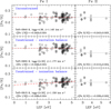 |
Fig. 1 Illustration of the three methods employed in the case of the differential analysis of α Cen A withthe line list of Bensby et al. (2014). Upper panels: unconstrained analysis requiring both excitation and ionisation equilibrium of iron; middle panels: constrained analysis assuming excitation balance of Fe I; bottom panels: constrained analysis assuming ionisation balance of iron. The dotted horizontal lines indicate the mean iron abundances, while the red dashed lines show the fit to the Fe I abundances as a function of LEP. |
4.3 Computation of uncertainties
Various sources of abundance uncertainties were considered. First, there are those related to the determination of the atmospheric parameters (Teff, log g, and ξ). The effect on the abundances was examined by altering one of the parameters by its uncertainty, while keeping the other two fixed. To estimate the uncertainty in Teff, for instance, we considered the range over which the slope of the relation between the Fe I abundances and LEP is consistent with zero within the uncertainties. As the parameters of the model are interdependent, however, changes in one of them are necessarily accompanied by variations in the other two, and covariance terms also need to be taken into account. Accordingly, in turn two of the parameters were also adjusted while the third one was varied by the relevant uncertainty. Once again, the analysis was repeated using this new set of parameters to estimate the impact on the abundances. Second, we explored to what extent the choice of another family of model atmospheres affects the results. To this end, we redetermined the abundances using the line list of Meléndez et al. (2014), but with Kurucz models computed with the ATLAS9 code ported under Linux (Sbordone 2005). The largest differences are found for α Cen B, but even in that case they appear to be small (Kurucz – MARCS): Δ Teff = +5 K, Δ log g = +0.02 dex, and abundance ratios deviating by less than 0.02 dex. Third, the line-to-line scatter was taken into account. A rather generous value of 0.05 dex (it is typically 0.03 dex) was assumed when only one line was used for a given ion. The final uncertainty was taken as thequadratic sum of all these various errors.
We made use of HARPS spectra with a resolving power degraded from R ~ 115 000 to 65 000 (see Sect. 3.1). We repeated the unconstrained analysis of α Cen A using the original spectra and the line list of Meléndez et al. (2014), but found negligible differences compared to the default results (e.g. abundances deviating by less than 0.01 dex).
5 Results
5.1 Stellar parameters
As a preamble, it was mentioned previously that the parameters of the targets differ significantly from solar. It is therefore unclear as to whether a differential analysis relative to the Sun actually improves the precision/accuracy of the results. To investigate this point, a standard analysis (i.e. without a joint analysis of the solar spectrum) was also undertaken. The results are presented in Table B.1. We compare in Fig. 2 (upper panels) our Teff and log g estimates to those obtained from less model-dependent techniques, namely interferometry and asteroseismology, respectively (see Sect. 4.2). Let us first discuss α Cen A. For the three methods considered, there is an overall good agreement between our results and the reference ones6. Even though the choice of the line list can lead to quite different parameters in the unconstrained case (covering a full range of 110 K and 0.29 dex for Teff and logg, respectively), the metallicity exhibits a relatively small scatter with all values being identical to within 0.06 dex. The constrained analysis assuming ionisation balance yields more precise Teff values (by a factor ~2.5), but this is not the case when enforcing excitation balance. The situation is quite different for α Cen B. First, the choice of theline list has a more profound effect on the results of the unconstrained analysis. Overall, there is also evidence for a systematic underestimation of logg at the ~0.2 dex level. Even in that case, however, [Fe/H] is nearly identical and as precisely determined as in α Cen A. There is an outstanding dependence between Teff and logg that illustrates the well-known degeneracy between the determination of these two quantities through spectroscopy alone. One would hope that fixing log g would break the degeneracy and increase the precision of the Teff determination. This is indeed what is observed when ionisation equilibrium is enforced. In sharp contrast, fulfilling excitation balance provides very unsatisfactory results. In most cases, it is even impossible to reach convergence because the Fe I abundances exhibit a noticeable trend as a function of the line strength whatever the microturbulence adopted. Similar problems have been encountered in the literature for relatively cool dwarfs (e.g. Jofré et al. 2014).
As can be seen in Fig. 2 (lower panels) in the case of α Cen A, the choice of the line list becomes basically irrelevant when a differential analysis between two stars with similar parameters is performed. Nearly identical parameters are obtained and the metallicity distributions are strongly peaked. This is especially true when ionisation balance is assumed, that is, the [Fe/H] values differ by less than a mere 0.015 dex. Once again, a different picture is obtained for α Cen B. Most importantly, there does not seem to be much benefit in performing a differential analysis (compare lower and upper panels). This distinct behaviour compared to α Cen A may reflect the fact that, α Cen B being significantly cooler than the Sun, systematic effects (e.g. inadequacies in the atmosphere structure) are not efficiently erased through a differential analysis. The iron line lists selected are made up of features whose formation may be quite different in terms of, for example, depth in the photosphere or sensitivity to departures from LTE. This could explain why the results depend on the choice of the diagnostic lines even in the case of a differential analysis. The mismatch in terms of parameters with respect to the Sun could also be one of the reasons contributing to a line-to-line scatter almost twice as large in α Cen B compared to α Cen A (typically 0.036 vs. 0.019 dex). In general, as for the standard analysis, a constrained analysis requiring ionisation balance performs much better.
In summary, we can draw the following conclusions:
-
The spectroscopic parameters are in general in satisfactory agreement with the presumably more accurate values derived from interferometry and asteroseismology, but there is evidence that logg is underestimated on average by ~0.2 dex in α Cen B.
-
There is a dramatic improvement in the precision of the results when a differential analysis is enforced for α Cen A. In contrast, there is apparently little benefit, if any, for α Cen B. This is interpreted as being due to parameters that depart significantly from solar in the latter case.
-
The choice of the line list has very little effect on the results when two stars with similar parameters are analysed in a differential way.
-
Fulfilling iron ionisation balance increases the precision of the results for the constrained analysis of Sun-like dwarfs. This approach should clearly be preferred over that requiring excitation equilibrium, especially for cool stars where convergence issues might be encountered.
-
All analyses yield consistent metallicities and lead to a robust value, [Fe/H] ~ +0.23 dex, which comfortably lies within the commonly accepted range for this system (0.20–0.25 dex; Sect. 6.1).
Now, the question arises as to what parameters should be adopted for the abundance analysis. First, based on the arguments presented above the results of the standard analysis can be regarded as less precise (at least for α Cen A) andare therefore discarded. Second, we ignore the constrained results assuming excitation equilibrium.A sound assumption could then be to adopt the results of the differential, constrained analysis assuming ionisation balance. However, as can be seen in Fig. 2, the [Fe/H] values for α Cen B show a relatively large spread and reach suspiciously high values (up to +0.34 dex). Although we have argued that the constrained results are generally more precise, it should also be kept in mind that they are not necessarily more accurate. The common belief that freezing logg improves the performance of spectroscopic analyses has been questioned (e.g. Smalley 2014). This is an important issue in the era of large stellar samples with asteroseismic data, which has certainly not yet received the attention it deserves. However, this cannot be meaningfully addressed with our limited dataset. We finally decided for the determination of the metal abundances to proceed with the parameters derived from the differential, unconstrained analysis (Table B.2). We note that our philosophy differs from that sometimes adopted in the literature (e.g. in the framework of the Gaia-ESO survey; Smiljanic et al. 2014) in that our abundances are not derived assuming a single set of recommended parameters. Instead, the abundances for a given line list are derived adopting the corresponding parameters, and are eventually combined to yield the final values.
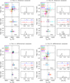 |
Fig. 2 Results of the classical (top) and differential (bottom) analyses of α Cen A (left) and α Cen B (right). Various analyses are considered (see Sect. 4.2): unconstrained (top panels), constrained assuming excitation balance (middle panels), and constrained assuming ionisation balance (bottom panels). The Teff and log g values obtained for each line list are shown with a different colour. The vertical and horizontal dashed lines indicate the 1σ range encompassed by the reference Teff and log g values (Sect. 4.2). The black error bars indicate the weighted mean of all the results (the position along the y-axis in the middle and bottom panels is shifted for clarity). The full results can be found in Tables B.1 and B.2. |
5.2 Chemical abundances
The abundances obtained for each line list are given for α Cen A and B in Tables B.3 and B.4, respectively. We only consider in the following the final abundances obtained from averaging these values (Table 1), as described in Sect. 4.2. The Fe, Si, Ca, Sc, Ti, and Cr abundances are derived from lines pertaining to two ionisation stages. For iron, the final value we adopt is the average weighted by the inverse variance of the Fe I- and Fe II-based abundances. For the other elements, we only consider abundances yielded by Si I, Ca I, Sc II, Ti I, and Cr I, as they are based on more features and exhibit a reduced line-to-line scatter. Ionisation balance is fulfilled for all of these species. The only exceptions are calcium and chromium in α Cen B. The origin of the Ca II and Cr II overabundances is unclear, but might arise from blends affecting the very few weak diagnostic lines. The non-LTE corrections for the features investigated are expected to be small (Bergemann & Cescutti 2010; Mashonkina et al. 2017).
As explained in Sect. 4.2, we did not carry out a differential analysis of one binary component relative to the other. To assess any differences in their chemical properties, we therefore simply subtracted the abundances of the two stars with respectto the Sun. However, we did trim the line lists to a common set of features before this operation, even thoughit leads to negligible differences (at most 0.011 dex). The results are given in Table 1.
The surface gravity of α Cen B appears to be slightly underestimated (Sect. 5.1). To estimate the impact on the abundances, we considered two groups of results: those obtained with two line lists that lead to logg close to the seismic value (Reddy et al. 2003; Biazzo et al. 2012) and two that lead to log g underestimated by ~0.2 dex (Morel et al. 2014; Meléndez et al. 2014). In all cases, Teff is close to the reference value. The abundance ratios of the two groups differ on average by less than 0.01 dex. It is therefore unlikely that the bias in logg strongly affects the conclusions presented in the following.
The impact of departures from LTE can be estimated on a star-to-star basis for about half of the elements studied. We made use of Spectrum Tools7 to interpolate the Fe I, Mg I, Si I, Ti I, Mn I, and Co I corrections for the relevant parameters (taken from Table 1, except for the logg of α Cen B for which we adopt the asteroseismic value because the spectroscopic one is slightly underestimated). We restrict ourselves to lines used in both components. The non-LTE calculations are discussed in Bergemann et al. (2010, 2012, 2013, 2015); Bergemann (2011), and Bergemann & Gehren (2008), respectively. The differential corrections (α Cen A or B relative to the Sun) for Fe I are nearly negligible (less than 0.01 dex) and are known to be even smaller for Fe II (e.g. Bergemann et al. 2012). This supports the assumption of LTE for the determination of the stellar parameters. The departures affecting Na I were evaluated in the same way, but with the interactive tool INSPECT8. The calculations are described in Lind et al. (2011). For the O I triplet, we adopt the values computed for α Cen AB by Ramírez et al. (2013). Other literature sources used are: Takeda & Honda (2005, C I), Nordlander & Lind (2017, Al I), Mashonkina et al. (2017, Ca I), Takeda et al. (2005, Zn I), and Korotin et al. (2015, Ba II). In these last cases, the coarseness of the grids only allows a rough estimate to be derived (e.g. the star-to-star Al I corrections only reflect the dependence with Teff; Nordlander & Lind 2017). Furthermore, we caution that our mean differential corrections are only representative given that data are only available for a subset of all the lines used. These corrections appear to be small and are discussed further in Sect. 6.3.2.
It was shown by Thompson et al. (2017) that the strengths of the temperature-sensitive photospheric features in α Cen B slightly vary depending on the activity level. Our spectrum was obtained when the star was in a moderately active state corresponding to an activity level a few times that of the Sun, as diagnosed by the ratio of the X-ray to bolometric luminosities (Ayres 2015). It is unlikely that activity-related phenomena significantly bias our results, but the analysis of various spectra taken along the ~8 yr activity cycle would certainly be illuminating. This issue is irrelevant for α Cen A, as it was caught during a deep activity minimum (Ayres 2015).
6 Discussion
6.1 Chemical properties of α Cen AB
We find that the abundance pattern of both stars is not scaled solar. Several elements are significantly enhanced (e.g. Na, Ni; see below), whereas others (especially the heaviest ones) are underabundant. The depletion of the neutron-capture elements (e.g. Y, Ba) will be used in Sect. 6.2 to put constraints on the age of the system. The slight (~0.06 dex) oxygen depletion is also noteworthy, but it is in line with the behaviour of the O I triplet-based LTE abundances as a function of [Fe/H] seen in FGK stars (Ramírez et al. 2013). Broadly speaking, all elements have abundances as expected for nearby, solar-like dwarfs of that metallicity, including an upturn in [Na/Fe] and [Ni/Fe] for supersolar [Fe/H] (e.g. Adibekyan et al. 2012; Bensby et al. 2014; Brewer et al. 2016).
Our study confirms a sodium and nickel excess in both stars (e.g. Neuforge-Verheecke & Magain 1997 and Porto de Mello et al. 2008). There exists an intriguingly tight relation between the [Ni/Fe] and [Na/Fe] abundance ratios in solar analogues at near-solar metallicity, which may be related to the fact that the Na and Ni yields of Type II supernovae are both functions of the neutron excess (Nissen 2015). A correlation is also seen in the data of Ramírez et al. (2014) for late F dwarfs and metal-rich solar analogues. As shown in Fig. 3, the two components of α Cen have larger [Ni/Fe] and [Na/Fe] values than solar analogues at near-solar metallicity, but seem to follow the same linear trend.
The elemental number ratios C/O and Mg/Si recently received particular attention because they have been claimed to control the mineralogy of extrasolar terrestrial planets (e.g. Suárez-Andrés et al. 2018, and references therein). A knowledge of the C/O and Mg/Si ratios in α Cen AB would constrain the value in Proxima Cen, with potential consequences for our understanding of the structure and composition of its planet (Brugger et al. 2016). Relative to solar, we determine C/O = 1.18 ± 0.07 and 1.18 ± 0.17 in α Cen A and B, respectively. For Mg/Si, we obtain 0.98 ± 0.06 and 1.02 ± 0.11, respectively. Correcting for departures from LTE (Sect. 5.2) leads to negligible differences, except for the C/O ratio in α Cen B, which is lowered by ~15%. Our results suggest that any putative terrestrial planets in α Cen have a composition not vastly different from those in our solar system.
Let us now compare our results to previous ones in the literature. We restrict ourselves to spectroscopic studies that derived the chemical composition of both components (Edvardsson 1988; Neuforge-Verheecke & Magain 1997; Allende Prieto et al. 2004; Gilli et al. 2006; Porto de Mello et al. 2008; Bruntt et al. 2010; Jofré et al. 2015; Luck 2018). We ignore the early study of England (1980), as it is plagued by large uncertainties and does not yield useful constraints. On the other hand, other works (e.g. Valenti & Fischer 2005) only derived the abundances of a few elements. Finally, we do not discuss the study of α Cen by Feltzing & Gonzalez (2001) because it duplicates to a large extent that of Neuforge-Verheecke & Magain (1997), using the same EWs, atomic data, and atmospheric parameters. The stellar parameters adopted by the eight selected studies are summarised in Table 2. It should be noted that several analyses are not self-consistent, as the atmosphericparameters could be taken from other works (e.g. Edvardsson 1988) or not derived from spectroscopy (e.g. Allende Prieto et al. 2004). The abundance patterns (including that from our study) are shown for both stars in Fig. 4 as a function of the 50% condensation temperature for a solar-system-composition gas (Tc; Lodders 2003). Adopting Tc values appropriate to more metal-rich material is unlikely to affect our conclusions, as they are systematically and only slightly offset (Lodders 2003; but see Bond et al. 2010). Also shown are the abundance differences between the two components as a function of Tc.
One of our most important results is that the abundance pattern of the two components is identical within the errors. The largest discrepancy is observed for [Y/Fe] at a significance level of ~2.5σ (Table 1). The mean abundance differences (A – B) are: ⟨Δ[X/H]⟩ = –0.008 ± 0.037 dex and ⟨Δ[X/Fe]⟩ = –0.021 ± 0.038 dex, where X represents a given species. The false alarm probability for the [X/Fe] data of the two stars to be uncorrelated is ~0.4% based on the computation of the generalised Kendall’s τ correlation coefficient. The size of the sample is exceedingly small, but we also find that the distribution of the Δ[X/Fe] values is statistically indistinguishable from a normal distribution centred at zero and with a standard deviation corresponding to our median uncertainty (σ ~ 0.037 dex).
The effects of microscopic diffusion are larger in α Cen A because of its thinner outer convective envelope. As gravitational settling largely dominates over radiative levitation, α Cen B should be less depleted in metals at the surface. Namely, we expect the mean abundance difference, ⟨Δ[X/H]⟩, defined above to be negative. This is only hinted at by our data, but any changes arising from diffusion can probably be accommodated by our uncertainties. The models of Deal et al. (2015) for C, Mg, and Fe indicate abundance differences of only ~0.002 dex for the binary components of 16 Cyg with a mass difference of 0.04 M⊙ and an age (6.4 Gyrs) comparable to that of α Cen (see Sect. 6.2). Deviations of ~0.02 dex for Mg, Ti, Fe, and Ni are suggested by the computations of Michaud et al. (2004) for solar-metallicity, FG dwarfs with the same age as above and a mass difference more appropriate to our case (~0.17 M⊙; Kervella et al. 2016). Finally, the uncalibrated models of α Cen AB by Turcotte & Christensen-Dalsgaard (1998) also lead to differences of this magnitude for the numerous metals they investigated.
The similarity between the chemical pattern of the two components was also pointed out by Neuforge-Verheecke & Magain (1997) based on data of similar precision (see Fig. 4), but our larger number of elements puts this conclusion on a firmer footing. We do not see any clear reasons to disregard their results, as was done by Hinkel & Kane (2013) who combined a selection of abundance results in the literature. We note that Hinkel & Kane (2013) inferred iron abundances ([Fe/H] = +0.28 and +0.31 dex for α Cen A and B, respectively) that are significantly larger than ours or, more generally, those in the literature (see Table 2). The studies of Allende Prieto et al. (2004) and Bruntt et al. (2010) suggest that α Cen B is overabundant in metals at the ~0.12 dex level (see Fig. 4). However, the Teff values adopted by Allende Prieto et al. (2004) and, to a much lesser extent, Bruntt et al. (2010) are lower than our or previous spectroscopic estimates (Table 2). Probably more telling is the fact that they are also lower than the interferometric measurements (Sect. 4.2) by ~270 and ~70 K, respectively. It is therefore tempting to associate these putative metallicity differences to a Teff scale that is too cool; see Ramírez et al. (2010) for further evidence indicating that the Teff values derived from colour indices by Allende Prieto et al. (2004) are underestimated. The even larger metallicity offset (~0.18 dex) found by Luck (2018) requires another explanation. It may arise from the very low microturbulence adopted for α Cen B (ξ = 0.25 km s−1).
Another way to look at differences between our results and previous ones is provided by Fig. 5. We only consider here elements with at least three measurements available from the studies listed in Table 2. Noticeable discrepancies are apparent for C, V, Co, and Cu. However, for carbon we find a better agreement between the abundance of the two components. The last three elements are affected by HFS effects, which sometimes seem to have been ignored (e.g. Gilli et al. 2006). This may explain the V, Co, and Cu overabundances reported in α Cen B where HFS corrections are particularly large.
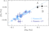 |
Fig. 3 Variation of [Ni/Fe] as a function of [Na/Fe] for solar analogues (Nissen 2015) and stars in the Kepler asteroseismic Legacy sample (Lund et al. 2017; Silva Aguirre et al. 2017) analysed by Nissen et al. (2017). All stars have –0.15 ≲ [Fe/H] ≲ +0.15. The dashed line shows the linear fit derived by Nissen (2015). The position of α Cen A and B is indicated as filled squares. |
Stellar parameters adopted by previous abundance studies in the literature.
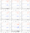 |
Fig. 4 Comparison between our abundance patterns and previous ones in the literature (Edvardsson 1988; Neuforge-Verheecke & Magain 1997; Luck 2018; Allende Prieto et al. 2004; Gilli et al. 2006; Porto de Mello et al. 2008; Bruntt et al. 2010; Jofré et al. 2015). For elementswith abundances corresponding to two ionisation stages, we followed the procedure outlined in Sect. 5.2. The results are shown as a function of Tc (Lodders 2003). For each study, the metal abundances of α Cen A and B relative to hydrogen, [X/H], are shown in the top and middle panels, respectively. A dashed line is drawn at [Fe/H]. Bottom panel: abundance differences, Δ [X/H], between α Cen A and B. To guide the eye, a dashed line is drawn at Δ[X/H] = 0. The dotted line indicates the mean difference, while the grey strip shows the corresponding 1σ uncertainties. For Edvardsson (1988), Porto de Mello et al. (2008) and our study, the uncertainties for elements other than iron refer to [X/Fe], not [X/H]. However, they are expected to be representative. |
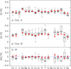 |
Fig. 5 Comparison between our abundances and those from previous studies (listed in Table 2) for elements with at least three measurements available. The vertical dashed line connects the extreme values found. The box covers the first to third quartile of the literature data, while the thick horizontal line inside the box shows the median. Our results are overplotted as red, filled circles. To guide the eye, a dotted line is drawn in the bottom panel at Δ [X/H] = 0. Our uncertainties for elements other than iron refer to [X/Fe], not [X/H]. However, they are expected to be representative. |
6.2 Age of the system from abundance indicators
Following the work of da Silva et al. (2012), recent high-precision studies of solar twins/analogues at near-solar metallicities (–0.15 ≲ [Fe/H] ≲ +0.15) have unveiled remarkable correlations between some abundance ratios and isochrone ages (e.g. Nissen 2015, 2016). Their robustness is supported by the fact that independent studies making use of different abundance data and sets of isochrones provide nearly identical relations. Ages derived from isochrone fitting are notoriously known to be model-dependent and prone to large uncertainties. However, quantitatively similar correlations are also found for stars in the Kepler Legacy sample (Lund et al. 2017; Silva Aguirre et al. 2017) with asteroseismic ages uncertain to within 10–20% (Nissen et al. 2017)9. The distinctbehaviour shown by elements produced through different nucleosynthesis channels strongly suggests that the abundance-age trends are intimately linked to the chemical evolution of the Galaxy (e.g. Spina et al. 2016a).
Of particular usefulness as age indicators are [Y/Mg] and [Y/Al], which show a tight and steep decline as a function of look-back time (Nissen 2015, 2016; Spina et al. 2016a, 2018; Tucci Maia et al. 2016). The correlation is interpreted as arising from a varying enrichment of the interstellar medium (ISM) in these two elements as the Galaxy evolves. For instance, the α-element magnesium is produced through core-collapse supernova events in the early Galaxy, while the s-process element yttrium is released in the ISM mainly through the winds of low-mass AGB stars (e.g. Bisterzo et al. 2014) over much longer time scales. The correlation extends over ~10 Gyrs and the age scatter is at most 1 Gyr for a given abundance ratio. Furthermore, the relations seem to be obeyed by distinct stellar populations (e.g. thin- and thick-disc stars; Nissen 2015), although this needs to be investigated further.
We considered various isochrone age-abundance calibrations to estimate the age of α Cen AB based on the [Y/Mg] and [Y/Al] ratios (Nissen 2016; Tucci Maia et al. 2016; Spina et al. 2018). The quadratic relations of Spina et al. (2018) were used, as the authors claim that they provide a significantly better fit to their data. The results are provided in Table 3. We regard the ages derived for α Cen A (~6.2 Gyrs) as more reliable, not only because of the smaller error bars, but also because they are likely less affectedby systematic effects (e.g. non-LTE corrections) arising from departures from the solar parameters.
Although the dependencies are more complex and not as clear, ages determined from abundance ratios relative to iron can valuably complement the [Y/Mg]- and [Y/Al]-based values. For ten metals with a reasonably well-defined behaviour and covering a sufficient abundance range (C, Mg, Al, Si, Sc, Ti, Cu, Zn, Y, and Ba), we determine an age for α Cen A of 5.7 ± 0.8 Gyrs from the linear relations of Nissen (2016). A different interpretation of the data was proposed by Spina et al. (2016a) who favoured hyperbolic fits with a turnover at intermediate ages to the abundance-age relations of many elements. Using the appropriate fitting functions (either linear or hyperbolic), we obtain an age of 6.6 ± 1.2 Gyrs for seven elements. No hyperbolic solutions could be obtained for three elements in common with Nissen (2016): Si, Cu, and Zn10. Linear relations based on a larger sample of solar analogues were recently proposed by Bedell et al. (2018). For five of the ten species above (Mg, Al, Ti, Y, and Ba), we obtain an age of 6.3 ± 1.3 Gyrs, while for the others the values exceed the validity range of the calibrations (8 Gyrs) by 1.3 Gyr on average. This further strengthens the case for a system older than solar.
In summary, we infer an age of ~6 Gyrs for α Cen. This value is fullycompatible with that determined by several theoretical studies that performed an asteroseismic modelling of both components. These works are based on p-mode frequencies derived from CORALIE (Thoul et al. 2003; Eggenberger et al. 2004; Miglio & Montalbán 2005) or UVES/UCLES (Y"i"ld"i"z 2011) RV time series. However, an approximately solar age was found from CORALIE (Thévenin et al. 2002) and HARPS (Bazot et al. 2016) data. Our results are not in sharp disagreement with this conclusion considering the relatively large error bars, but they tend to support instead a system slightly more evolved than the Sun. Discrepant ages for the two components are found by Lundkvist et al. (2014). It should be noted that the asteroseismic age of α Cen A is quite uncertain and depends on whether the optimal model presents a small convective core or not (see, e.g. Bazot et al. 2016). A seismic study cannot be performed for Proxima Cen since M stars are not known to present any observables that arise from pulsations (e.g. Rodríguez et al. 2016). A wide range of ages is inferred for α Cen AB from gyrochronology (4.0–9.2 Gyrs; Barnes 2007; Mamajek & Hillenbrand 2008; Delorme et al. 2011; Epstein & Pinsonneault 2014; Angus et al. 2015). The age we derive is broadly consistent with the rotation period of Proxima Cen (~83 d; Benedict et al. 1998) according to the calibrations for late M dwarfs by Engle & Guinan (2018).
We caution that the accuracy of ages relying on spectroscopic indicators is still not well established. In particular, as discussed by Feltzing et al. (2017), there is a significant spread in [Y/Mg] for a given age in nearby dwarfs, with more metal-poor stars displaying lower ratios. We therefore anticipate that, in virtue of their metal-rich nature, the [Y/Mg]-based age we derive for α Cen AB is affected by this effect and is likely to be revised upwards. However, with the caveat that the metallicity dependence of the calibrations remains to be fully understood and quantified, we speculate that the corrections are slight (tentatively of the order of ~0.5 Gyr). No discernable variation in the [Y/Mg]-age relation is indeed found when splitting samples of solar analogues in two metallicity bins separated by Δ[Fe/H] ~0.15 dex (Tucci Maia et al. 2016). Another concern is that α Cen B is clearly not a solar analogue. The data of Nissen et al. (2017) show that stars significantly warmer (up to 6350 K) and more evolved (logg down to 3.95 dex) than the Sun follow the relations defined by solar analogues, albeit with a larger scatter (see also Adibekyan et al. 2016). This suggests that the calibrations may reasonably be used for stars falling formally outside the solar analogue category provided the mismatch in terms of parameters is not too large (but see Slumstrup et al. 2017 who argue that the relations might also be valid for solar-metallicity, core-helium burning giants). The Mg I and Al I abundances are largely insensitive to non-LTE effects: the differential corrections do not exceed 0.01 dex. The departures from LTE for Y II are unknown, but are probably small if one considers that this ionisation stage is by far the most populated.
Stellar ages derived from [Y/Mg] and [Y/Al] abundance ratios.
6.3 Abundance patterns in the context of planetary formation
6.3.1 Planets in α Cen
Before discussing the implications of our results in the context of planetary formation in α Cen, let us review the attempts made to detect substellar-mass companions in the system.
Being our closest neighbour, the system is a prime target for the detection of planets that could possibly host life. Issues related to the accretion of planetesimals and stability of planets in close binaries (the semi-major axis is only about 23.4 AU) cannot be ignored (e.g. Kraus et al. 2016). However, circumstellar planets in tight binaries do exist (e.g. Ortiz et al. 2016, and references therein). It has also been claimed that the presence of Proxima Cen orbiting the inner pair is unlikely to prevent planet formation (Worth & Sigurdsson 2016).
If one accepts that the conditions are indeed favourable to planet formation and stability in α Cen AB, then it might be expected that the components harbour Jupiter-like companions in view of the higher occurrence of close-in giant planets around metal-rich stars (e.g. Gonzalez 1997). However, such planets have remained elusive in spite of considerable observational effort (e.g. Endl et al. 2001; Kervella et al. 2006; Zhao et al. 2018). The failure of high-resolution imaging and sensitive RVmonitoring, which probe different regions around the stars, to detect giant planets down to a few Jupiter masses casts seriousdoubts on their existence.
Evidence for lower-mass planets in α Cen AB is also inconclusive. The discovery of a planet with a minimum mass of 1.3 M⊕ orbiting Proxima Cen was recently announced (Anglada-Escudé et al. 2016). It was followed by the detection of cold dust belts and possiblya warm dust reservoir that could be leftovers from a past planetary formation episode (Anglada et al. 2017; Ribas et al. 2017). Furthermore, the presence of a Keplerian signal was confirmed by Damasso & Del Sordo (2017) from a re-analysis of the RV data of Anglada-Escudé et al. (2016). Hints of transit-like events were also found (Blank et al. 2018, and references therein). However, there is currently little observational evidence for planets of this kind in α Cen AB. There have been claims of a close-in, Earth-mass planet in α Cen B (α Cen Bb) through thedetection of very low-amplitude RV variations in HARPS data (K ~ 0.5 m s−1; Dumusque et al. 2012). Unfortunately, independent re-analyses of these data demonstrated that the weak planetary signal, which is close to the detection capability of the instrument and buried in “jitter” noise arising from magnetic activity, is very likely spurious (Hatzes 2013; Rajpaul et al. 2015, 2016). The possible existence of a small-size transiting planet, α Cen Bc, was recently reported (Demory et al. 2015), but needs confirmation. Infrared emission from dusty debris discs has not been detected in α Cen AB (Wiegert et al. 2014). From the theoretical side, several studies have investigated the formation and dynamics of planets in the binary system, but quite often reached different conclusions owing to the complexity of the problem (e.g. Thébault et al. 2008, and references therein). The recognition that the detection of terrestrial planets might be within reach through an extremely intensive and precise RV monitoring (e.g. Guedes et al. 2008; Eggl et al. 2013) has triggered a number of ambitious campaigns (e.g. Endl et al. 2015).
To summarise, even though the existence of a low-mass planet in Proxima Cen seems quite secure, there are only observational hints of a transiting planet in α Cen B and no indications that α Cen A hosts a planet at all.
6.3.2 Trends with condensation temperature
Meléndez et al. (2009) and Ramírez et al. (2009) convincingly demonstrated that the Sun is depleted at the 20% level in species that can easily condensate in dust grains (refractory elements) relative to volatiles when compared to most solar analogues. They showed that only ~15% of all the stars in their samples have an abundance pattern closely resembling that of the Sun or are poorer in refractories. Moreover, the level of depletion is an increasing function of Tc. They proposed that a similar behaviour in other stars might provide indirect evidence for the existence of rocky material trapped in terrestrial planets (see also, e.g. Ramírez et al. 2010). Chambers (2010) and Meléndez et al. (2012) went a step further by claiming that an extremely precise abundance analysis can help to constrain the total mass and relative amount of Earth-like and meteoritic material around the star. How gas giant planets fit into this scenario is not completely clear, but it has been postulated that their formation could lead to a global metal deficiency in the parent star and not necessarily a discernable trend in the [X/Fe]–Tc relation (Ramírez et al. 2014).
Over the last decade, a great number of studies have investigated whether a correlation in solar-like dwarfs between metal abundances and condensation temperature could indeed be a relic of a past planetary formation episode. Although appealing, this claim has not received wide support (e.g. González Hernández et al. 2013). The biggest blow against this interpretation is arguably the lack of any clear refractory depletion in a small sample of Kepler targets that are known to host Earth-size planets (Schuler et al. 2015). Nonetheless, the authors warned that their conclusions are still subject to a number of uncertainties, such as those related to the architecture of the planetary systems or the chemical evolution of the Galaxy (the age spread in their sample is at least 3 Gyrs). Conversely, Liu et al. (2016b) claimed that such a depletion of refractory elements is, as expected, present in the terrestrial planet host Kepler-10.
One of the major obstacles that prevents one from clearly establishing a causal link between the depletion of refractory elements and the formation of terrestrial planets is that it is very difficult to define clear-cut and well-defined samples of bona fide single stars and planet hosts. Even in confirmed hosts, the planet census is not complete and there is a very strong bias against finding Earth-like planets. To complicate the matter further, the predictions are sensitive to a number of uncertain assumptions; for example, the size of the convective envelope when the circumstellar material was accreted (e.g. Chambers 2010) or the chemical composition of super-Earth and Neptune-like planets (e.g. Rogers 2015). Furthermore, the opposite effect (i.e. an excess of refractory elements) can result from the infall of planets onto the star (e.g. Spina et al. 2015). All these difficulties conspire to make a clear interpretation of the abundance pattern in exoplanet host stars difficult and very often ambiguous. Although the debate is still far from being settled, some general conclusions are, however, emerging. First and foremost, trends shown by solar twins/analogues between [X/Fe] and Tc appear to primarily be an age effect imprinted by the chemical evolution of the Galaxy (e.g. Adibekyan et al. 2014; Nissen 2015; Spina et al. 2016b). Superimposed on these [X/Fe]–Tc trends are second-order effects unrelated to age that introduce additional scatter. They arise either from the sequestration/ingestion of planetarymaterial (e.g. Meléndez et al. 2009; Ramírez et al. 2014), radiative cleansing of dust in the primordial gas cloud (e.g. Önehag et al. 2014; Liu et al. 2016a), and/or dust-gas segregation in protoplanetary discs (e.g. Gaidos 2015).
To remove the effect of Galactic chemical evolution (GCE), we corrected the abundances using the age–[X/Fe] relations of Nissen (2016). For V, Co, Zr, and Ce, which were not included in this study, we adopted the relations of Bedell et al. (2018). We assumed an age of 6 ± 1 Gyrs (Sect. 6.2). The corrected abundances are given in Table 1. Although the corrections are small given the similar age of α Cen and the Sun, they are noticeable at this level of precision and lead to a reduced scatter (e.g. from 0.040 to 0.029 dex in α Cen A), as can be seen in Fig. 6.
To examine the relationship between [X/Fe] corrected for GCE effects and Tc, we only consider refractory elements with Tc > 900 K, as these species are better indicators of phenomena related to planetary formation (e.g. Bedell et al. 2018). In addition, the abundances of volatiles (C, O, and Zn) are based on a few lines that are particularly sensitive to some physical effects not considered here (e.g. departures from LTE for the O I triplet). These elements with uncertain abundances and much lower Tc values would strongly bias the slopes obtained. We also ignore Na and Ni whose exceptionally high abundance in α Cen (Fig. 3) is unlikely to be related to planetary formation. For consistency, we finally discard Mn and Ce in order to have exactly the same set of elements for α Cen A and B. We finally end up with 13 elements. The best-fit parameters obtained from a linear regression taking the errors in the abundance ratios into account are given in Table 4. A linear fit is expected to constitute a good representation of the data, as some differential studies of stellar twins in binaries (where the highest precision is reached) have shown that the element-to-element scatter relative to the regression line is comparable to the measurement errors (e.g. Ramírez et al. 2015). As seen in Fig. 6, the non-LTE effects discussed in Sect. 5.2 are generally small and unlikely to significantly bias the [X/Fe]-Tc trends.
The data for α Cen A hint at an even larger depletion of refractory elements compared to the Sun. However, the [X/Fe]–Tc slope is very close (at the 1.2σ level) to solar and a linear fit with a zero slope is nearly as good based on χ2 statistics. In contrast, the slope differs from that typical of solar analogues over the same Tc range and corrected for GCE effects (~+7.3 × 10⁻⁵ dex K−1; Bedell et al. 2018) at a much higher confidence level (~3.2σ)11. Indeed, the slope for α Cen A is comparable to the lowest found among the 68 solar analogues studied by Bedell et al. (2018). However, although a fit to our data using the relation for solar analogues after adjusting the intercept to minimise the residuals is significantly worse (χ2 ratio of ~2.2), it cannot be ruled out on statistical grounds. Forα Cen B, no conclusions can be drawn in view of the larger error bars: trends similar to that in the Sun or in solar analogues are both possible. The situation for the abundance differences is similar to that encountered for α Cen A. Although a similar behaviour for the two components is preferred, a fit using the typical relation for solar analogues is also statistically acceptable: slope deviating by 2.6σ from the best-fit one and increase in χ2 by a factor of about 1.9. It is worth recalling that the data discussed here are sensitive to the treatment of GCE effects. However, similar conclusions are obtained when using the GCE corrections of Bedell et al. (2018) for all elements.
Significant progress in our understanding of the [X/Fe]–Tc trends may come from comparing the abundance pattern of binary components because any differences found are free from environmental or age effects (the latter assuming coevality). To put our results in perspective, we compare in Fig. 7 the abundance differences we find in α Cen to those reported in the literature for planet-host binaries also analysed differentially. Some of them only have one star that is known to host a planet (HAT-P-1, HAT-P-4, 16 Cyg, and HD 80606/HD 80607), while others have planets orbiting both the primary and secondary (WASP-94, XO-2, HD 133131, and HD 20781/HD 20782). These are Jupiter-mass giants in all cases. The only exception is HD 20781, which harbours two super-Earth and two Neptune-like companions (Udry et al. 2017). A noticeable element-to-element scatter is observed for systems where the Teff mismatch between the stars is the largest: α Cen (ΔTeff = 640 K) and HD 20781/HD 20782 (ΔTeff = 465 K). The deviations are much lower for most other systems that all have Δ Teff ≲ 200 K. This suggests that much of the scatter in α Cen arises from the mismatch in spectral type between the binary components. If present, a clear metallicity offset and/or a well-defined [X/H]–Tc behaviour, as seen in XO-2, must be buried in the noise. Narrowing down the uncertainties to the appropriate level would require a full treatment of 3D/non-LTE effects and diffusion for all elements; a formidable task well beyond our current capabilities. However, a large offset in bulk metallicity of ~0.1 dex, as claimed in HAT-P-4 and attributed to planet engulfment (Saffe et al. 2017) can be ruled out. The large scatter observed for this system is puzzling considering that the components are extremely close in terms of Teff and log g. Although departures in the chemical patterns of binary components can likely be ascribed to the existence of planets, as shown in Fig. 7, the reverse is not necessarily true. This is nicely illustrated by HAT-P-1 and HD 80606/HD 80607; despite a close-in giant planet orbiting one of the two stars, the abundance patterns are strikingly similar (to within 0.01 dex: Liu et al. 2014, 2018).
We now explore the possibility that a putative planet that initially formed in either α Cen A or B was swallowed during the star’s evolution. This can occur because of planet-planet scattering (e.g. Mustill et al. 2015) or secular perturbations in multiple stellar systems (e.g. Petrovich 2015). The latter process operates on timescales that are dramatically longer than the former and is therefore more likely to leave an imprint on the surface abundances because of the much thinner stellar convective zone (CZ) at old ages (see below).
The change in metallicity, Δ[M/H], resulting from planet ingestion can be written as (e.g. Teske et al. 2016b)
![Mathematical equation: \begin{equation*} \mathrm{\Delta} \mathrm{[M/H]} = \log \left[ \frac{M_{\mathrm{CZ}}+ M_{\mathrm{p}} \times [(Z/X)_{\mathrm{p}}/(Z/X)_{\mathrm{CZ}}]}{M_{\mathrm{CZ}}+M_{\mathrm{p}}} \right],\end{equation*}](/articles/aa/full_html/2018/07/aa33125-18/aa33125-18-eq5.png) (3)
(3)
where Mp and MCZ are the masses of the planet and of the CZ at the time of accretion, respectively.  and
and  are the corresponding metal content relative to hydrogen. The resulting change in metallicity is a crude estimate (likely an upper limit) assuming no readjustment of the whole internal structure and that the metal-rich accreted material is instantaneously diluted within the convective envelope and does not sink because of, for example, thermohaline convection (e.g. Garaud 2011; Théado & Vauclair 2012). To estimate the variation of the CZ mass as the stars evolve, we use Yale models (Spada et al. 2013) computed for a mixing-length parameter αMLT = 1.875, [Fe/H] = +0.30, and masses of 0.95 and 1.10 M⊙ (the measured values are 1.1055 and 0.9373 M⊙ for α Cen A and B, respectively; Kervella et al. 2016). In addition, we follow Thorngren et al. (2016) and assume that the planet and stellar metallicities are related via
  /
/ ~ 9.7 ×
  . Three illustrative cases are examined with planet masses corresponding to that of Neptune, Saturn, and Jupiter. The results are shown in Fig. 8.
A modification of the surface bulk metallicity would be easier to detect in α Cen A because of its larger mass and therefore thinner CZ. Standard evolutionary models indicate that the late accretion of at least one Saturn mass would lead to detectable changes. One would therefore be tempted to conclude that the ingestion of such an amount of planetary material since the time when the stars reached their present-day CZs (30–40 Myrs after star formation) can be ruled out. This conclusion can be extended to earlier times if alternative models where the CZ shrinks faster are considered (Baraffe & Chabrier 2010). An anomalous abundance for the fragile elements Li and Be may also be taken as evidence for a swallowing event, although the quantitative effect is still very much controversial (e.g. Deal et al. 2015). No attempts were made here to derive the lithium abundance from Li I λ670.8 because of its extreme weakness, but other studies indicate that the Li content in the two stars differs by ~0.7 dex, with α Cen B being more depleted (Luck 2018). For Be, it amounts to ~0.6 dex (Primas et al. 1997). These discrepancies may be accounted for by the different internal structure, but detailed calculations are warranted. Accretion of circumstellar material is the best candidate to account for the clear departures between the abundance patterns of the components in the old 16 Cyg and XO-2 systems (Fig. 7). Although this suggests that extra-mixing mechanisms are perhaps less efficient at erasing the imprint of such processes than currently thought, they are still likely to play an important role and to affect the conclusions above (e.g. Garaud 2011; Théado & Vauclair 2012). The uncertain impact of mixing on the predictions should be kept in mind.
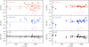 |
Fig. 6 Left panels: abundance patterns as a function of Tc (Lodders 2003). The metal abundances of α Cen A and B relative to iron, [X/Fe], are shown in the top and middle panels, respectively. Bottom panel: abundance differences, Δ[X/Fe], between α Cen A and B. To guide the eye, a dashed line is drawn at Δ[X/Fe] = 0. The dotted line in the bottom panel indicates the mean difference, while the grey strip shows the corresponding 1σ uncertainties. The vertical lines in the bottom of each panel show the non-LTE corrections (non-LTE minus LTE). A horizontal tick at the bottom or top of the line indicates a negative or positive correction, respectively. Values lower than ~0.01 dex are shown with a dot. Right panels: same as left panels, but after correction for GCE. The solid lines are the best linear fits to the refractory elements (Tc > 900 K; Table 4). The elements not included in the fit (Na, Mn, Ni, and Ce) are shown as open circles. The dashed line shows the typical GCE-corrected relationship found for solar analogues (Bedell et al. 2018) after adjustment of the intercept to minimise the residuals. |
Results of the weighted, linear [X/Fe]–Tc fits after correction for GCE effects.
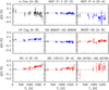 |
Fig. 7 Comparison between our abundance differences and those reported in the literature for planet-host binaries also analysed differentially. Systems with only one or the two components known to host planets are shown with blue and red symbols, respectively. For systems with only one planet host, the convention is star without planet minus star with planet. Source of the data: HAT-P-1 (Liu et al. 2014), HAT-P-4 (Saffe et al. 2017), 16 Cyg (Tucci Maia et al. 2014), HD 80606/HD 80607 (Liu et al. 2018), WASP-94 (Teske et al. 2016a), XO-2 (Ramírez et al. 2015), HD 133131 (Teske et al. 2016b), and HD 20781/HD 20782 (Mack et al. 2014). For elements with abundances corresponding to two ionisation stages, we followed the procedure outlined in Sect. 5.2. For WASP-94, we considered the dataset with strong lines excluded (see Teske et al. 2016a). |
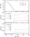 |
Fig. 8 Upperpanel: variation of the mass of the CZ as a function of stellar age. Middle and bottom panels: variation in bulk metallicity corresponding to the ingestion of a planet as a function of stellar age. Three illustrative cases are shown: Jupiter-, Saturn-, and Neptune-mass planets. |
7 Conclusions
We derive a robust estimate for the metallicity of the system: [Fe/H] ~ +0.23 dex. The 3D hydrodynamical simulations of α Cen A by Bigot et al. (2008) intriguingly suggest a lower metallicity ([Fe/H] ~ +0.16 dex) than found by most 1D spectroscopic studies, but the results are regarded by the authors as still preliminary. Further calculations are urgently needed. An inspection of the iron abundances reported in the literature for Proxima Cen reveals an uncomfortably wide spread: +0.16 ± 0.20 (Neves et al. 2014), –0.03 ± 0.09 (Maldonado et al. 2015), –0.07 ± 0.14 (Passegger et al. 2016), and +0.08 ± 0.12 (Zhao et al. 2018). Abundances of a few elements (including Na, Ti, and Fe) were also reported by Pavlenko et al. (2017) to be roughly consistent with solar. The relatively large study-to-study scatter illustrates the difficulties in properly modelling the spectra and atmospheres of very cool stars, even though it is one of the rare M stars benefiting from a Teff constraint coming from interferometric measurements (Demory et al. 2009). Our study suggests with a high degree of confidence that the iron abundance of the main pair lies in the range +0.20 < [Fe/H] < +0.25. At first glance, this appears to be at odds with the values determined for Proxima Cen, although the lack of consensus for the M star prevents one from reaching definitive conclusions. Further investigations are needed to clarify whether the iron abundance of Proxima Cen fulfils the constraint imposed by α Cen AB. Otherwise, the identification of α Cen as a triple system formed out of the same natal cloud may need to be questioned.
We find evidence in α Cen A for a [X/Fe]–Tc trend much more similar to what is observed in the Sun than in the majority of solar analogues (no conclusion can be drawn for α Cen B owing to the larger error bars). However, we refrain from associating this finding to the sequestration of rocky material in small bodies orbiting the star. First, a behaviour similar to that of solar analogues cannot be firmly ruled out on statistical grounds. More importantly, a causal link between planetary formation and [X/Fe]–Tc trends is still hotly debated (e.g. Schuler et al. 2015). Another difficulty is related to the removal of GCE effects. The system has thin-disc kinematics (e.g. Ramírez et al. 2007) and a Galactic orbit that lies within the solar annulus: mean Galactocentric distance of ~8.3 kpc, eccentricity of ~0.07, and maximum distance above the Galactic plane of ~310 pc (Casagrande et al. 2011). However, its high metallicity is only shared by a few per cent of all stars in the solar neighbourhood (e.g. Casagrande et al. 2011) and cannot be attributed to a young age. It is conceivable that α Cen migrated from the inner Galaxy (e.g. Kordopatis et al. 2015) where the nucleosynthesis history could have been different from that experienced by the bulk of the nearby solar analogues used to define the GCE trends. It might also imply that the Sun and α Cen formed in different environments and suffered various amounts of dust radiative cleansing (see, e.g. Önehag et al. 2014; Liu et al. 2016a).
We find that the abundance patterns of α Cen A and B are remarkably similar considering that both line-formation (e.g. 3D/non-LTE) or other physical (e.g. diffusion) effects likelyintroduce significant random and systematic differences. The similarity between the abundance patterns of the two stars suggests that the late (i.e. after the stars have reached their present-day CZs) accretion of large amounts (above about one Saturn mass) of metal-rich material by either star did not occur, but this conclusion is very sensitive to the details of how this material was subsequently transported downwards.
Assuming coeval formation, we also suggest an age of about ~6 Gyrs for thecool tertiary Proxima Cen and its planet. Obviously, this conclusion fully relies on the assumption that the three stars formed together and Proxima Cen was not captured, an issue which is still not completely settled (Reipurth & Mikkola 2012; Feng & Jones 2018).
Acknowledgements
The author acknowledges financial support from Belspo for contract PRODEX PLATO. He wishes to thank Megan Bedell for sending her abundance data prior to publication and Chris Sneden for his help with the blends driver in MOOG. The useful comments from the anonymous referee are also greatly appreciated. This research made use of NASA’s Astrophysics Data System Bibliographic Services and the SIMBAD database operated at CDS, Strasbourg (France).
Appendix A Lines selected and EW measurements
Table A.1 provides the spectral features selected for each line list and the EW measurements.
Lines selected and EW measurements.
Appendix B Stellar parameters and chemical abundances obtained for each line list
Tables B.1 and B.2 provide for each line list the stellar parameters obtained from the classical and differential analysis, respectively. The chemical abundances of α Cen A and B aregiven in Tables B.3 and B.4, respectively.
Stellar parameters obtained from the classical analysis.
Stellar parameters obtained from the differential analysis.
Chemical abundances of α Cen A obtained from the differential, unconstrained analysis.
Chemical abundances of α Cen B obtained from the differential, unconstrained analysis.
References
- Adibekyan, V. Z., Sousa, S. G., Santos, N. C., et al. 2012, A&A, 545, A32 [NASA ADS] [CrossRef] [EDP Sciences] [Google Scholar]
- Adibekyan, V. Z., González Hernández, J. I., Delgado Mena, E., et al. 2014, A&A, 564, L15 [NASA ADS] [CrossRef] [EDP Sciences] [Google Scholar]
- Adibekyan, V., Delgado-Mena, E., Figueira, P., et al. 2016, A&A, 592, A87 [NASA ADS] [CrossRef] [EDP Sciences] [Google Scholar]
- Allende Prieto, C., Barklem, P. S., Lambert, D. L., & Cunha, K. 2004, A&A, 420, 183 [NASA ADS] [CrossRef] [EDP Sciences] [Google Scholar]
- Anglada, G., Amado, P. J., Ortiz, J. L., et al. 2017, ApJ, 850, L6 [NASA ADS] [CrossRef] [Google Scholar]
- Anglada-Escudé, G., Amado, P. J., Barnes, J., et al. 2016, Nature, 536, 437 [NASA ADS] [CrossRef] [PubMed] [Google Scholar]
- Angus, R., Aigrain, S., Foreman-Mackey, D., & McQuillan, A. 2015, MNRAS, 450, 1787 [NASA ADS] [CrossRef] [Google Scholar]
- Asplund, M., Grevesse, N., Sauval, A. J., & Scott, P. 2009, ARA&A, 47, 481 [NASA ADS] [CrossRef] [Google Scholar]
- Ayres, T. R. 2015, AJ, 149, 58 [NASA ADS] [CrossRef] [Google Scholar]
- Baraffe, I., & Chabrier, G. 2010, A&A, 521, A44 [NASA ADS] [CrossRef] [EDP Sciences] [Google Scholar]
- Barnes, S. A. 2007, ApJ, 669, 1167 [NASA ADS] [CrossRef] [Google Scholar]
- Barnes, R., Deitrick, R., Luger, R., et al. 2016, ArXiv e-prints [arXiv:1608.06919] [Google Scholar]
- Bazot, M., Christensen-Dalsgaard, J., Gizon, L., & Benomar, O. 2016, MNRAS, 460, 1254 [NASA ADS] [CrossRef] [Google Scholar]
- Bedell, M., Meléndez, J., Bean, J. L., et al. 2014, ApJ, 795, 23 [NASA ADS] [CrossRef] [Google Scholar]
- Bedell, M., Bean, J. L., Melendez, J., et al. 2018, ApJ, submitted, [arXiv:1802.02576] [Google Scholar]
- Benedict, G. F., McArthur, B., Nelan, E., et al. 1998, AJ, 116, 429 [NASA ADS] [CrossRef] [Google Scholar]
- Bensby, T., Feltzing, S., & Oey, M. S. 2014, A&A, 562, A71 [NASA ADS] [CrossRef] [EDP Sciences] [Google Scholar]
- Bergemann, M. 2011, MNRAS, 413, 2184 [NASA ADS] [CrossRef] [Google Scholar]
- Bergemann, M., & Cescutti, G. 2010, A&A, 522, A9 [NASA ADS] [CrossRef] [EDP Sciences] [Google Scholar]
- Bergemann, M., & Gehren, T. 2008, A&A, 492, 823 [NASA ADS] [CrossRef] [EDP Sciences] [Google Scholar]
- Bergemann, M., Pickering, J. C., & Gehren, T. 2010, MNRAS, 401, 1334 [NASA ADS] [CrossRef] [Google Scholar]
- Bergemann, M., Lind, K., Collet, R., Magic, Z., & Asplund, M. 2012, MNRAS, 427, 27 [NASA ADS] [CrossRef] [Google Scholar]
- Bergemann, M., Kudritzki, R.-P., Würl, M., et al. 2013, ApJ, 764, 115 [NASA ADS] [CrossRef] [Google Scholar]
- Bergemann, M., Kudritzki, R.-P., Gazak, Z., Davies, B., & Plez, B. 2015, ApJ, 804, 113 [NASA ADS] [CrossRef] [Google Scholar]
- Biazzo, K., D’Orazi, V., Desidera, S., et al. 2012, MNRAS, 427, 2905 [NASA ADS] [CrossRef] [Google Scholar]
- Biazzo, K., Gratton, R., Desidera, S., et al. 2015, A&A, 583, A135 [NASA ADS] [CrossRef] [EDP Sciences] [Google Scholar]
- Bigot, L., Kervella, P., Thévenin, F., & Ségransan, D. 2006, A&A, 446, 635 [NASA ADS] [CrossRef] [EDP Sciences] [Google Scholar]
- Bigot, L., Thévenin, F., & Kervella, P. 2008, Mem. Soc. Astron. It., 79, 670 [NASA ADS] [Google Scholar]
- Bisterzo, S., Travaglio, C., Gallino, R., Wiescher, M., & Käppeler, F. 2014, ApJ, 787, 10 [NASA ADS] [CrossRef] [Google Scholar]
- Blanco-Cuaresma, S., Soubiran, C., Heiter, U., & Jofré, P. 2014a, A&A, 569, A111 [NASA ADS] [CrossRef] [EDP Sciences] [Google Scholar]
- Blanco-Cuaresma, S., Soubiran, C., Jofré, P., & Heiter, U. 2014b, A&A, 566, A98 [NASA ADS] [CrossRef] [EDP Sciences] [Google Scholar]
- Blank, D. L., Feliz, D., Collins, K. A., et al. 2018, AJ, 155, 228 [NASA ADS] [CrossRef] [Google Scholar]
- Bond, J. C., O’Brien, D. P., & Lauretta, D. S. 2010, ApJ, 715, 1050 [NASA ADS] [CrossRef] [Google Scholar]
- Boyajian, T. S., von Braun, K., van Belle, G., et al. 2013, ApJ, 771, 40 [NASA ADS] [CrossRef] [Google Scholar]
- Brewer, J. M., Fischer, D. A., Valenti, J. A., & Piskunov, N. 2016, ApJS, 225, 32 [NASA ADS] [CrossRef] [Google Scholar]
- Brugger, B., Mousis, O., Deleuil, M., & Lunine, J. I. 2016, ApJ, 831, L16 [NASA ADS] [CrossRef] [Google Scholar]
- Bruntt, H., Bedding, T. R., Quirion, P.-O., et al. 2010, MNRAS, 405, 1907 [NASA ADS] [Google Scholar]
- Casagrande, L., Schönrich, R., Asplund, M., et al. 2011, A&A, 530, A138 [NASA ADS] [CrossRef] [EDP Sciences] [Google Scholar]
- Chambers, J. E. 2010, ApJ, 724, 92 [NASA ADS] [CrossRef] [Google Scholar]
- Chen, Y. Q., Nissen, P. E., Zhao, G., Zhang, H. W., & Benoni, T. 2000, A&AS, 141, 491 [NASA ADS] [CrossRef] [EDP Sciences] [Google Scholar]
- Creevey, O. L., Thévenin, F., Basu, S., et al. 2013, MNRAS, 431, 2419 [NASA ADS] [CrossRef] [Google Scholar]
- Damasso, M., & Del Sordo, F. 2017, A&A, 599, A126 [NASA ADS] [CrossRef] [EDP Sciences] [Google Scholar]
- da Silva, R., Porto de Mello, G. F., Milone, A. C., et al. 2012, A&A, 542, A84 [NASA ADS] [CrossRef] [EDP Sciences] [Google Scholar]
- Deal, M., Richard, O., & Vauclair, S. 2015, A&A, 584, A105 [NASA ADS] [CrossRef] [EDP Sciences] [Google Scholar]
- Delorme, P., Collier Cameron, A., Hebb, L., et al. 2011, MNRAS, 413, 2218 [NASA ADS] [CrossRef] [Google Scholar]
- Demory, B.-O., Ségransan, D., Forveille, T., et al. 2009, A&A, 505, 205 [NASA ADS] [CrossRef] [EDP Sciences] [Google Scholar]
- Demory, B.-O., Ehrenreich, D., Queloz, D., et al. 2015, MNRAS, 450, 2043 [NASA ADS] [CrossRef] [Google Scholar]
- Desidera, S., Gratton, R. G., Scuderi, S., et al. 2004, A&A, 420, 683 [NASA ADS] [CrossRef] [EDP Sciences] [Google Scholar]
- Desidera, S., Gratton, R. G., Lucatello, S., & Claudi, R. U. 2006, A&A, 454, 581 [NASA ADS] [CrossRef] [EDP Sciences] [Google Scholar]
- Dumusque, X., Pepe, F., Lovis, C., et al. 2012, Nature, 491, 207 [NASA ADS] [CrossRef] [PubMed] [Google Scholar]
- Edvardsson, B. 1988, A&A, 190, 148 [NASA ADS] [Google Scholar]
- Eggenberger, P., Charbonnel, C., Talon, S., et al. 2004, A&A, 417, 235 [NASA ADS] [CrossRef] [EDP Sciences] [Google Scholar]
- Eggl, S., Pilat-Lohinger, E., Funk, B., Georgakarakos, N., & Haghighipour, N. 2013, MNRAS, 428, 3104 [NASA ADS] [CrossRef] [Google Scholar]
- Endl, M., Kürster, M., Els, S., Hatzes, A. P., & Cochran, W. D. 2001, A&A, 374, 675 [NASA ADS] [CrossRef] [EDP Sciences] [Google Scholar]
- Endl, M., Bergmann, C., Hearnshaw, J., et al. 2015, Int. J. Astrobiol., 14, 305 [CrossRef] [Google Scholar]
- England, M. N. 1980, MNRAS, 191, 23 [NASA ADS] [Google Scholar]
- Engle, S. G., & Guinan, E. F. 2018, Research Notes of the American Astronomical Society, 2, 34 [Google Scholar]
- Epstein, C. R., & Pinsonneault, M. H. 2014, ApJ, 780, 159 [NASA ADS] [CrossRef] [Google Scholar]
- Feltzing, S., & Gonzalez, G. 2001, A&A, 367, 253 [NASA ADS] [CrossRef] [EDP Sciences] [Google Scholar]
- Feltzing, S., Howes, L. M., McMillan, P. J., & Stonkutė, E. 2017, MNRAS, 465, L109 [NASA ADS] [CrossRef] [Google Scholar]
- Feng, F., & Jones, H. R. A. 2018, MNRAS, 473, 3185 [NASA ADS] [CrossRef] [Google Scholar]
- French, V. A., & Powell, A. L. T. 1971, Royal Greenwich Observatory Bulletins, 173, 63 [NASA ADS] [Google Scholar]
- Gaidos, E. 2015, ApJ, 804, 40 [NASA ADS] [CrossRef] [Google Scholar]
- Garaud, P. 2011, ApJ, 728, L30 [NASA ADS] [CrossRef] [Google Scholar]
- Gilli, G., Israelian, G., Ecuvillon, A., Santos, N. C., & Mayor, M. 2006, A&A, 449, 723 [NASA ADS] [CrossRef] [EDP Sciences] [Google Scholar]
- Gonzalez, G. 1997, MNRAS, 285, 403 [NASA ADS] [CrossRef] [Google Scholar]
- González Hernández, J. I., Delgado-Mena, E., Sousa, S. G., et al. 2013, A&A, 552, A6 [NASA ADS] [CrossRef] [EDP Sciences] [Google Scholar]
- Guedes, J. M., Rivera, E. J., Davis, E., et al. 2008, ApJ, 679, 1582 [NASA ADS] [CrossRef] [Google Scholar]
- Guenther, D. B., & Demarque, P. 2000, ApJ, 531, 503 [NASA ADS] [CrossRef] [Google Scholar]
- Gustafsson, B., Edvardsson, B., Eriksson, K., et al. 2008, A&A, 486, 951 [NASA ADS] [CrossRef] [EDP Sciences] [Google Scholar]
- Hatzes, A. P. 2013, ApJ, 770, 133 [NASA ADS] [CrossRef] [Google Scholar]
- Heiter, U., Jofré, P., Gustafsson, B., et al. 2015, A&A, 582, A49 [NASA ADS] [CrossRef] [EDP Sciences] [PubMed] [Google Scholar]
- Hinkel, N. R., & Kane, S. R. 2013, MNRAS, 432, L36 [NASA ADS] [CrossRef] [Google Scholar]
- Hinkle, K., Wallace, L., Valenti, J., & Harmer, D. 2000, Visible and Near Infrared Atlas of the Arcturus Spectrum 3727-9300 A (San Francisco: ASP) [Google Scholar]
- Huber, D., Chaplin, W. J., Christensen-Dalsgaard, J., et al. 2013, ApJ, 767, 127 [NASA ADS] [CrossRef] [Google Scholar]
- Jofré, P., Heiter, U., Soubiran, C., et al. 2014, A&A, 564, A133 [NASA ADS] [CrossRef] [EDP Sciences] [Google Scholar]
- Jofré, P., Heiter, U., Soubiran, C., et al. 2015, A&A, 582, A81 [NASA ADS] [CrossRef] [EDP Sciences] [Google Scholar]
- Kervella, P., Thévenin, F., Ségransan, D., et al. 2003, A&A, 404, 1087 [NASA ADS] [CrossRef] [EDP Sciences] [Google Scholar]
- Kervella, P., Thévenin, F., Coudé du Foresto, V., & Mignard, F. 2006, A&A, 459, 669 [NASA ADS] [CrossRef] [EDP Sciences] [Google Scholar]
- Kervella, P., Mignard, F., Mérand, A., & Thévenin, F. 2016, A&A, 594, A107 [NASA ADS] [CrossRef] [EDP Sciences] [Google Scholar]
- Kervella, P., Bigot, L., Gallenne, A., & Thévenin, F. 2017a, A&A, 597, A137 [NASA ADS] [CrossRef] [EDP Sciences] [Google Scholar]
- Kervella, P., Thévenin, F., & Lovis, C. 2017b, A&A, 598, L7 [NASA ADS] [CrossRef] [EDP Sciences] [Google Scholar]
- Kjeldsen, H., Bedding, T. R., Arentoft, T., et al. 2008, ApJ, 682, 1370 [NASA ADS] [CrossRef] [Google Scholar]
- Kordopatis, G., Binney, J., Gilmore, G., et al. 2015, MNRAS, 447, 3526 [NASA ADS] [CrossRef] [Google Scholar]
- Korotin, S. A., Andrievsky, S. M., Hansen, C. J., et al. 2015, A&A, 581, A70 [NASA ADS] [CrossRef] [EDP Sciences] [Google Scholar]
- Kraus, A. L., Ireland, M. J., Huber, D., Mann, A. W., & Dupuy, T. J. 2016, AJ, 152, 8 [NASA ADS] [CrossRef] [Google Scholar]
- Lind, K., Asplund, M., Barklem, P. S., & Belyaev, A. K. 2011, A&A, 528, A103 [Google Scholar]
- Liu, F., Asplund, M., Ramírez, I., Yong, D., & Meléndez, J. 2014, MNRAS, 442, L51 [NASA ADS] [CrossRef] [Google Scholar]
- Liu, F., Asplund, M., Yong, D., et al. 2016a, MNRAS, 463, 696 [NASA ADS] [CrossRef] [Google Scholar]
- Liu, F., Yong, D., Asplund, M., et al. 2016b, MNRAS, 456, 2636 [NASA ADS] [CrossRef] [Google Scholar]
- Liu, F., Yong, D., Asplund, M., et al. 2018, A&A, 614, A138 [NASA ADS] [CrossRef] [EDP Sciences] [Google Scholar]
- Lodders, K. 2003, ApJ, 591, 1220 [NASA ADS] [CrossRef] [Google Scholar]
- Luck, R. E. 2018, AJ, 155, 111 [NASA ADS] [CrossRef] [Google Scholar]
- Lund, M. N., Silva Aguirre, V., Davies, G. R., et al. 2017, ApJ, 835, 172 [CrossRef] [Google Scholar]
- Lundkvist, M., Kjeldsen, H., & Silva Aguirre V. 2014, A&A, 566, A82 [NASA ADS] [CrossRef] [EDP Sciences] [Google Scholar]
- Mack, III, C. E., Schuler, S. C., Stassun, K. G., & Norris, J. 2014, ApJ, 787, 98 [NASA ADS] [CrossRef] [Google Scholar]
- Maldonado, J., Affer, L., Micela, G., et al. 2015, A&A, 577, A132 [NASA ADS] [CrossRef] [EDP Sciences] [Google Scholar]
- Mamajek, E. E., & Hillenbrand, L. A. 2008, ApJ, 687, 1264 [NASA ADS] [CrossRef] [Google Scholar]
- Mashonkina, L., Sitnova, T., & Belyaev, A. K. 2017, A&A, 605, A53 [NASA ADS] [CrossRef] [EDP Sciences] [Google Scholar]
- Meléndez, J., Asplund, M., Gustafsson, B., & Yong, D. 2009, ApJ, 704, L66 [NASA ADS] [CrossRef] [Google Scholar]
- Meléndez, J., Bergemann, M., Cohen, J. G., et al. 2012, A&A, 543, A29 [NASA ADS] [CrossRef] [EDP Sciences] [Google Scholar]
- Meléndez, J., Ramírez, I., Karakas, A. I., et al. 2014, ApJ, 791, 14 [NASA ADS] [CrossRef] [Google Scholar]
- Michaud, G., Richard, O., Richer, J., & VandenBerg, D. A. 2004, ApJ, 606, 452 [NASA ADS] [CrossRef] [EDP Sciences] [Google Scholar]
- Miglio, A., & Montalbán, J. 2005, A&A, 441, 615 [NASA ADS] [CrossRef] [EDP Sciences] [Google Scholar]
- Morel, T., Rainer, M., Poretti, E., Barban, C., & Boumier, P. 2013, A&A, 552, A42 [NASA ADS] [CrossRef] [EDP Sciences] [Google Scholar]
- Morel, T., Miglio, A., Lagarde, N., et al. 2014, A&A, 564, A119 [NASA ADS] [CrossRef] [EDP Sciences] [Google Scholar]
- Mustill, A. J., Davies, M. B., & Johansen, A. 2015, ApJ, 808, 14 [NASA ADS] [CrossRef] [Google Scholar]
- Neuforge-Verheecke, C., & Magain, P. 1997, A&A, 328, 261 [NASA ADS] [Google Scholar]
- Neves, V., Bonfils, X., Santos, N. C., et al. 2014, A&A, 568, A121 [NASA ADS] [CrossRef] [EDP Sciences] [Google Scholar]
- Nissen, P. E. 2015, A&A, 579, A52 [NASA ADS] [CrossRef] [EDP Sciences] [Google Scholar]
- Nissen, P. E. 2016, A&A, 593, A65 [NASA ADS] [CrossRef] [EDP Sciences] [Google Scholar]
- Nissen, P. E., Silva Aguirre, V., Christensen-Dalsgaard, J., et al. 2017, A&A, 608, A112 [NASA ADS] [CrossRef] [EDP Sciences] [Google Scholar]
- Nordlander, T., & Lind, K. 2017, A&A, 607, A75 [NASA ADS] [CrossRef] [EDP Sciences] [Google Scholar]
- Önehag, A., Gustafsson, B., & Korn, A. 2014, A&A, 562, A102 [NASA ADS] [CrossRef] [EDP Sciences] [Google Scholar]
- Ortiz, M., Reffert, S., Trifonov, T., et al. 2016, A&A, 595, A55 [NASA ADS] [CrossRef] [EDP Sciences] [Google Scholar]
- Pancino, E., Lardo, C., Altavilla, G., et al. 2017, A&A, 598, A5 [NASA ADS] [CrossRef] [EDP Sciences] [Google Scholar]
- Passegger, V. M., Wende-von Berg, S., & Reiners, A. 2016, A&A, 587, A19 [NASA ADS] [CrossRef] [EDP Sciences] [Google Scholar]
- Pavlenko, Y., Suárez Mascareño, A., Rebolo, R., et al. 2017, A&A, 606, A49 [NASA ADS] [CrossRef] [EDP Sciences] [Google Scholar]
- Petrovich, C. 2015, ApJ, 799, 27 [NASA ADS] [CrossRef] [Google Scholar]
- Porto de Mello, G. F., Lyra, W., & Keller, G. R. 2008, A&A, 488, 653 [NASA ADS] [CrossRef] [EDP Sciences] [Google Scholar]
- Pourbaix, D., & Boffin, H. M. J. 2016, A&A, 586, A90 [NASA ADS] [CrossRef] [EDP Sciences] [Google Scholar]
- Primas, F., Duncan, D. K., Pinsonneault, M. H., Deliyannis, C. P., & Thorburn, J. A. 1997, ApJ, 480, 784 [NASA ADS] [CrossRef] [Google Scholar]
- Quarles, B., & Lissauer, J. J. 2018, AJ, 155, 130 [NASA ADS] [CrossRef] [Google Scholar]
- Quintana, E. V., Lissauer, J. J., Chambers, J. E., & Duncan, M. J. 2002, ApJ, 576, 982 [NASA ADS] [CrossRef] [Google Scholar]
- Rajpaul, V., Aigrain, S., Osborne, M. A., Reece, S., & Roberts, S. 2015, MNRAS, 452, 2269 [NASA ADS] [CrossRef] [Google Scholar]
- Rajpaul, V., Aigrain, S., & Roberts, S. 2016, MNRAS, 456, L6 [NASA ADS] [CrossRef] [Google Scholar]
- Ramírez, I., Allende Prieto, C., & Lambert, D. L. 2007, A&A, 465, 271 [NASA ADS] [CrossRef] [EDP Sciences] [Google Scholar]
- Ramírez, I., Meléndez, J., & Asplund, M. 2009, A&A, 508, L17 [NASA ADS] [CrossRef] [EDP Sciences] [Google Scholar]
- Ramírez, I., Asplund, M., Baumann, P., Meléndez, J., & Bensby, T. 2010, A&A, 521, A33 [NASA ADS] [CrossRef] [EDP Sciences] [Google Scholar]
- Ramírez, I., Meléndez, J., Cornejo, D., Roederer, I. U., & Fish, J. R. 2011, ApJ, 740, 76 [NASA ADS] [CrossRef] [Google Scholar]
- Ramírez, I., Allende Prieto, C., & Lambert, D. L. 2013, ApJ, 764, 78 [NASA ADS] [CrossRef] [Google Scholar]
- Ramírez, I., Meléndez, J., & Asplund, M. 2014, A&A, 561, A7 [NASA ADS] [CrossRef] [EDP Sciences] [Google Scholar]
- Ramírez, I., Khanal, S., Aleo, P., et al. 2015, ApJ, 808, 13 [NASA ADS] [CrossRef] [Google Scholar]
- Rauer, H., Catala, C., Aerts, C., et al. 2014, Exp. Astron., 38, 249 [NASA ADS] [CrossRef] [Google Scholar]
- Reddy, B. E., Tomkin, J., Lambert, D. L., & Allende Prieto C. 2003, MNRAS, 340, 304 [NASA ADS] [CrossRef] [Google Scholar]
- Reipurth, B., & Mikkola, S. 2012, Nature, 492, 221 [Google Scholar]
- Ribas, I., Gregg, M. D., Boyajian, T. S., & Bolmont, E. 2017, A&A, 603, A58 [NASA ADS] [CrossRef] [EDP Sciences] [Google Scholar]
- Rodríguez, E., Rodríguez-López, C., López-González, M. J., et al. 2016, MNRAS, 457, 1851 [NASA ADS] [CrossRef] [Google Scholar]
- Rogers, L. A. 2015, ApJ, 801, 41 [NASA ADS] [CrossRef] [Google Scholar]
- Saffe, C., Jofré, E., Martioli, E., et al. 2017, A&A, 604, L4 [NASA ADS] [CrossRef] [EDP Sciences] [Google Scholar]
- Santos, N. C., Israelian, G., Mayor, M., et al. 2005, A&A, 437, 1127 [NASA ADS] [CrossRef] [EDP Sciences] [Google Scholar]
- Sbordone, L. 2005, Mem. Soc. Astron. It. Supp., 8, 61 [Google Scholar]
- Schuler, S. C., Vaz, Z. A., Katime Santrich, O. J., et al. 2015, ApJ, 815, 5 [NASA ADS] [CrossRef] [Google Scholar]
- Silva Aguirre, V., Lund, M. N., Antia, H. M., et al. 2017, ApJ, 835, 173 [NASA ADS] [CrossRef] [Google Scholar]
- Slumstrup, D., Grundahl, F., Brogaard, K., et al. 2017, A&A, 604, L8 [NASA ADS] [CrossRef] [EDP Sciences] [Google Scholar]
- Smalley, B. 2014, Determination of Atmospheric Parameters of B-, A-, F- and G-Type Stars eds. E. Niemczura, B. Smalley, & W. Pych (Cham: Springer International Publishing), 233 [Google Scholar]
- Smiljanic, R., Korn, A. J., Bergemann, M., et al. 2014, A&A, 570, A122 [NASA ADS] [CrossRef] [EDP Sciences] [Google Scholar]
- Smith, G., Edvardsson, B., & Frisk, U. 1986, A&A, 165, 126 [NASA ADS] [Google Scholar]
- Sneden, C. A. 1973, PhD Thesis, The University of Texas at Austin., USA [Google Scholar]
- Sousa, S. G., Santos, N. C., Mayor, M., et al. 2008, A&A, 487, 373 [NASA ADS] [CrossRef] [EDP Sciences] [MathSciNet] [Google Scholar]
- Spada, F., Demarque, P., Kim, Y.-C., & Sills, A. 2013, ApJ, 776, 87 [NASA ADS] [CrossRef] [Google Scholar]
- Spina, L., Palla, F., Randich, S., et al. 2015, A&A, 582, L6 [NASA ADS] [CrossRef] [EDP Sciences] [Google Scholar]
- Spina, L., Meléndez, J., Karakas, A. I., et al. 2016a, A&A, 593, A125 [NASA ADS] [CrossRef] [EDP Sciences] [Google Scholar]
- Spina, L., Meléndez, J., & Ramírez, I. 2016b, A&A, 585, A152 [NASA ADS] [CrossRef] [EDP Sciences] [Google Scholar]
- Spina, L., Meléndez, J., Karakas, A. I., et al. 2018, MNRAS, 474, 2580 [NASA ADS] [Google Scholar]
- Suárez-Andrés, L., Israelian, G., González Hernández, J. I., et al. 2018, A&A, 614, A84 [NASA ADS] [CrossRef] [EDP Sciences] [Google Scholar]
- Takeda, Y., & Honda, S. 2005, PASJ, 57, 65 [NASA ADS] [Google Scholar]
- Takeda, Y., Hashimoto, O., Taguchi, H., et al. 2005, PASJ, 57, 751 [NASA ADS] [Google Scholar]
- Teske, J. K., Ghezzi, L., Cunha, K., et al. 2015, ApJ, 801, L10 [NASA ADS] [CrossRef] [Google Scholar]
- Teske, J. K., Khanal, S., & Ramírez, I. 2016a, ApJ, 819, 19 [NASA ADS] [CrossRef] [Google Scholar]
- Teske, J. K., Shectman, S. A., Vogt, S. S., et al. 2016b, AJ, 152, 167 [NASA ADS] [CrossRef] [Google Scholar]
- Théado, S., & Vauclair, S. 2012, ApJ, 744, 123 [NASA ADS] [CrossRef] [Google Scholar]
- Thébault, P., Marzari, F., & Scholl, H. 2008, MNRAS, 388, 1528 [NASA ADS] [CrossRef] [Google Scholar]
- Thévenin, F., Provost, J., Morel, P., et al. 2002, A&A, 392, L9 [NASA ADS] [CrossRef] [EDP Sciences] [Google Scholar]
- Thompson, A. P. G., Watson, C. A., de Mooij, E. J. W., & Jess, D. B. 2017, MNRAS, 468, L16 [NASA ADS] [CrossRef] [Google Scholar]
- Thorngren, D. P., Fortney, J. J., Murray-Clay, R. A., & Lopez, E. D. 2016, ApJ, 831, 64 [NASA ADS] [CrossRef] [Google Scholar]
- Thoul, A., Scuflaire, R., Noels, A., et al. 2003, A&A, 402, 293 [NASA ADS] [CrossRef] [EDP Sciences] [Google Scholar]
- Tucci Maia, M., Meléndez, J., & Ramírez, I. 2014, ApJ, 790, L25 [NASA ADS] [CrossRef] [Google Scholar]
- Tucci Maia, M., Ramírez, I., Meléndez, J., et al. 2016, A&A, 590, A32 [NASA ADS] [CrossRef] [EDP Sciences] [Google Scholar]
- Turcotte, S., & Christensen-Dalsgaard, J. 1998, ESA SP, 418, 407 [NASA ADS] [Google Scholar]
- Udry, S., Dumusque, X., Lovis, C., et al. 2017, A&A, submitted, [arXiv:1705.05153] [Google Scholar]
- Valenti, J. A.,& Fischer, D. A. 2005, ApJS, 159, 141 [NASA ADS] [CrossRef] [MathSciNet] [Google Scholar]
- Wiegert, J., Liseau, R., Thébault, P., et al. 2014, A&A, 563, A102 [NASA ADS] [CrossRef] [EDP Sciences] [Google Scholar]
- Worth, R., & Sigurdsson, S. 2016, ApJ, 831, 170 [NASA ADS] [CrossRef] [Google Scholar]
- Y"i"ld"i"z, M. 2011, MNRAS, 412, 2571 [CrossRef] [Google Scholar]
- Zhao, L., Fischer, D. A., Brewer, J., Giguere, M., & Rojas-Ayala, B. 2018, AJ, 155, 24 [NASA ADS] [CrossRef] [Google Scholar]
See, e.g. ESO press release at: https://www.eso.org/public/unitedkingdom/news/eso1702/
Available at https://www.blancocuaresma.com/s/benchmarkstars. Two spectra are available for α Cen A. We decided to use the exposure with a slightly lower S/N because of a better blaze correction.
IRAF is distributed by the National Optical Astronomy Observatories, operated by the Association of Universities for Research in Astronomy, Inc., under cooperative agreement with the National Science Foundation.
Available at http://kurucz.harvard.edu/linelists.html
We do not adopt the potentially more precise estimates provided by the latter technique, as there are significant discrepancies in dynamical stellar masses between various studies (compare, e.g. Pourbaix & Boffin 2016 and Kervella et al. 2016).
We do not expect a perfect coincidence between our excitation/ionisation temperatures, which relate to the physical conditions prevailing in the iron line-formation zone, and the interferometric value, which is more directly tied to the definition of effective temperature.
Available online at: http://nlte.mpia.de.
Available online at: http://www.inspect-stars.com.
The new relations of Nissen et al. (2017) are not considered further because they are based on a mixture of ages derived from different techniques (isochrone fitting and asteroseismology). However, they do not noticeably differ from those assumed in our paper. Indeed, they lead to similar ages within the errors.
In a few cases, the ages we derive slightly exceed (by less than 0.8 Gyr) the domains of validity of the calibrations, which are 6 and 8 Gyrs for Nissen (2016) and Spina et al. (2016a), respectively. Because of the high Na and Ni abundances in α Cen AB compared to solar analogues (see Sect. 6.1), the [Na/Fe] and [Ni/Fe] ratios cannot be used. In any case, these ratios are poorly correlated with age (Spina et al. 2016a).
A deviation slightly more pronounced is found if Mn and Ce are taken into account.
All Tables
Chemical abundances of α Cen A obtained from the differential, unconstrained analysis.
Chemical abundances of α Cen B obtained from the differential, unconstrained analysis.
All Figures
|
Fig. 1 Illustration of the three methods employed in the case of the differential analysis of α Cen A withthe line list of Bensby et al. (2014). Upper panels: unconstrained analysis requiring both excitation and ionisation equilibrium of iron; middle panels: constrained analysis assuming excitation balance of Fe I; bottom panels: constrained analysis assuming ionisation balance of iron. The dotted horizontal lines indicate the mean iron abundances, while the red dashed lines show the fit to the Fe I abundances as a function of LEP. |
| In the text | |
|
Fig. 2 Results of the classical (top) and differential (bottom) analyses of α Cen A (left) and α Cen B (right). Various analyses are considered (see Sect. 4.2): unconstrained (top panels), constrained assuming excitation balance (middle panels), and constrained assuming ionisation balance (bottom panels). The Teff and log g values obtained for each line list are shown with a different colour. The vertical and horizontal dashed lines indicate the 1σ range encompassed by the reference Teff and log g values (Sect. 4.2). The black error bars indicate the weighted mean of all the results (the position along the y-axis in the middle and bottom panels is shifted for clarity). The full results can be found in Tables B.1 and B.2. |
| In the text | |
|
Fig. 3 Variation of [Ni/Fe] as a function of [Na/Fe] for solar analogues (Nissen 2015) and stars in the Kepler asteroseismic Legacy sample (Lund et al. 2017; Silva Aguirre et al. 2017) analysed by Nissen et al. (2017). All stars have –0.15 ≲ [Fe/H] ≲ +0.15. The dashed line shows the linear fit derived by Nissen (2015). The position of α Cen A and B is indicated as filled squares. |
| In the text | |
|
Fig. 4 Comparison between our abundance patterns and previous ones in the literature (Edvardsson 1988; Neuforge-Verheecke & Magain 1997; Luck 2018; Allende Prieto et al. 2004; Gilli et al. 2006; Porto de Mello et al. 2008; Bruntt et al. 2010; Jofré et al. 2015). For elementswith abundances corresponding to two ionisation stages, we followed the procedure outlined in Sect. 5.2. The results are shown as a function of Tc (Lodders 2003). For each study, the metal abundances of α Cen A and B relative to hydrogen, [X/H], are shown in the top and middle panels, respectively. A dashed line is drawn at [Fe/H]. Bottom panel: abundance differences, Δ [X/H], between α Cen A and B. To guide the eye, a dashed line is drawn at Δ[X/H] = 0. The dotted line indicates the mean difference, while the grey strip shows the corresponding 1σ uncertainties. For Edvardsson (1988), Porto de Mello et al. (2008) and our study, the uncertainties for elements other than iron refer to [X/Fe], not [X/H]. However, they are expected to be representative. |
| In the text | |
|
Fig. 5 Comparison between our abundances and those from previous studies (listed in Table 2) for elements with at least three measurements available. The vertical dashed line connects the extreme values found. The box covers the first to third quartile of the literature data, while the thick horizontal line inside the box shows the median. Our results are overplotted as red, filled circles. To guide the eye, a dotted line is drawn in the bottom panel at Δ [X/H] = 0. Our uncertainties for elements other than iron refer to [X/Fe], not [X/H]. However, they are expected to be representative. |
| In the text | |
|
Fig. 6 Left panels: abundance patterns as a function of Tc (Lodders 2003). The metal abundances of α Cen A and B relative to iron, [X/Fe], are shown in the top and middle panels, respectively. Bottom panel: abundance differences, Δ[X/Fe], between α Cen A and B. To guide the eye, a dashed line is drawn at Δ[X/Fe] = 0. The dotted line in the bottom panel indicates the mean difference, while the grey strip shows the corresponding 1σ uncertainties. The vertical lines in the bottom of each panel show the non-LTE corrections (non-LTE minus LTE). A horizontal tick at the bottom or top of the line indicates a negative or positive correction, respectively. Values lower than ~0.01 dex are shown with a dot. Right panels: same as left panels, but after correction for GCE. The solid lines are the best linear fits to the refractory elements (Tc > 900 K; Table 4). The elements not included in the fit (Na, Mn, Ni, and Ce) are shown as open circles. The dashed line shows the typical GCE-corrected relationship found for solar analogues (Bedell et al. 2018) after adjustment of the intercept to minimise the residuals. |
| In the text | |
|
Fig. 7 Comparison between our abundance differences and those reported in the literature for planet-host binaries also analysed differentially. Systems with only one or the two components known to host planets are shown with blue and red symbols, respectively. For systems with only one planet host, the convention is star without planet minus star with planet. Source of the data: HAT-P-1 (Liu et al. 2014), HAT-P-4 (Saffe et al. 2017), 16 Cyg (Tucci Maia et al. 2014), HD 80606/HD 80607 (Liu et al. 2018), WASP-94 (Teske et al. 2016a), XO-2 (Ramírez et al. 2015), HD 133131 (Teske et al. 2016b), and HD 20781/HD 20782 (Mack et al. 2014). For elements with abundances corresponding to two ionisation stages, we followed the procedure outlined in Sect. 5.2. For WASP-94, we considered the dataset with strong lines excluded (see Teske et al. 2016a). |
| In the text | |
|
Fig. 8 Upperpanel: variation of the mass of the CZ as a function of stellar age. Middle and bottom panels: variation in bulk metallicity corresponding to the ingestion of a planet as a function of stellar age. Three illustrative cases are shown: Jupiter-, Saturn-, and Neptune-mass planets. |
| In the text | |
Current usage metrics show cumulative count of Article Views (full-text article views including HTML views, PDF and ePub downloads, according to the available data) and Abstracts Views on Vision4Press platform.
Data correspond to usage on the plateform after 2015. The current usage metrics is available 48-96 hours after online publication and is updated daily on week days.
Initial download of the metrics may take a while.