| Issue |
A&A
Volume 604, August 2017
|
|
|---|---|---|
| Article Number | A32 | |
| Number of page(s) | 87 | |
| Section | Interstellar and circumstellar matter | |
| DOI | https://doi.org/10.1051/0004-6361/201730466 | |
| Published online | 31 July 2017 | |
The complexity of Orion: an ALMA view
I. Data and first results⋆,⋆⋆
1 LERMA & UMR 8112 du CNRS, Observatoire de Paris, PSL Research University, CNRS, Sorbonne Universités, UPMC Univ. Paris 06, 75014 Paris, France
e-mail: laurent.pagani@obspm.fr
2 Univ. Grenoble Alpes, CNRS, IPAG, 38000 Grenoble, France
3 INAF–Osservatorio Astrofisico di Arcetri, Largo E. Fermi 5, 50125 Florence, Italy
e-mail: cfavre@arcetri.astro.it
4 JPL, Pasadena, California, USA
e-mail: paul.f.goldsmith@jpl.nasa.gov
5 Department of Astronomy, University of Michigan, 311 West Hall, 1085 S. University Ave, Ann Arbor, MI 48109, USA
6 Department of Astronomy, University of Massachusetts, Amherst, MA 01003, USA
7 Harvard-Smithsonian Center for Astrophysics, Cambridge, Massachusetts, USA
Received: 19 January 2017
Accepted: 22 May 2017
Context. We wish to improve our understanding of the Orion central star formation region (Orion-KL) and disentangle its complexity.
Aims. We collected data with ALMA during cycle 2 in 16 GHz of total bandwidth spread between 215.1 and 252.0 GHz with a typical sensitivity of 5 mJy/beam (2.3 mJy/beam from 233.4 to 234.4 GHz) and a typical beam size of 1.̋7 × 1.̋0 (average position angle of 89°). We produced a continuum map and studied the emission lines in nine remarkable infrared spots in the region including the hot core and the compact ridge, plus the recently discovered ethylene glycol peak.
Methods. We present the data, and report the detection of several species not previously seen in Orion, including n- and i-propyl cyanide (C3H7CN), and the tentative detection of a number of other species including glycolaldehyde (CH2(OH)CHO). The first detections of gGg′ ethylene glycol (gGg′ (CH2OH)2) and of acetic acid (CH3COOH) in Orion are presented in a companion paper. We also report the possible detection of several vibrationally excited states of cyanoacetylene (HC3N), and of its 13C isotopologues. We were not able to detect the 16O18O line predicted by our detection of O2 with Herschel, due to blending with a nearby line of vibrationally excited ethyl cyanide. We do not confirm the tentative detection of hexatriynyl (C6H) and cyanohexatriyne (HC7N) reported previously, or of hydrogen peroxide (H2O2) emission.
Results. We report a complex velocity structure only partially revealed before. Components as extreme as −7 and +19 km s-1 are detected inside the hot region. Thanks to different opacities of various velocity components, in some cases we can position these components along the line of sight. We propose that the systematically redshifted and blueshifted wings of several species observed in the northern part of the region are linked to the explosion that occurred ~500 yr ago. The compact ridge, noticeably farther south displays extremely narrow lines (~1 km s-1) revealing a quiescent region that has not been affected by this explosion. This probably indicates that the compact ridge is either over 10 000 au in front of or behind the rest of the region.
Conclusions. Many lines remain unidentified, and only a detailed modeling of all known species, including vibrational states of isotopologues combined with the detailed spatial analysis offered by ALMA enriched with zero-spacing data, will allow new species to be detected.
Key words: ISM: clouds / ISM: structure / ISM: individual objects: Orion-KL (except planetary nebulae) / astrochemistry / molecular processes
This paper makes use of the following ALMA data: ADS/JAO.ALMA#2013.1.00533.S. ALMA is a partnership of ESO (representing its member states), NSF (USA) and NINS (Japan), together with NRC (Canada), NSC and ASIAA (Taiwan), and KASI (Republic of Korea), in cooperation with the Republic of Chile. The Joint ALMA Observatory is operated by ESO, AUI/NRAO and NAOJ.
The reduced ALMA data cubes as listed in Table 1 are available at the CDS via anonymous ftp to cdsarc.u-strasbg.fr (130.79.128.5) or via http://cdsarc.u-strasbg.fr/viz-bin/qcat?J/A+A/604/A32
© ESO, 2017
1. Introduction
The Orion region hosts two well-studied star forming sites, Orion A and Orion B. Orion A is subdivided into four clouds (Orion Molecular Cloud 1–4, OMC) and OMC1 holds the Kleinmann-Low Nebula (KL), often referred to as Orion-KL (but also numerous other names, as listed in SIMBAD1). The Orion-KL nebula is the nearest massive star forming region (distance equal to 388 pc ± 5 pc, Kounkel et al. 2017, in replacement of the previous value of 414 pc ± 7 pc, Sandstrom et al. 2007; Menten et al. 2007) and as such has attracted considerable attention and is the subject of thousands of publications. The core is complex with several remarkable sources, the hot core (HC), the compact ridge (CR), the extended ridge (ER), the plateau, numerous methyl formate (MF) peaks (Favre et al. 2011a), and other infrared/submillimeter peaks listed in many papers (e.g. Rieke et al. 1973; Robberto et al. 2005; Friedel & Weaver 2011), including three runaway objects: BN, I, and n (Gómez et al. 2005; Rodríguez et al. 2005, 2017). Among the studies aimed at identifying molecules in Orion, which is the reference source along with Sgr B2 in which to search for new species, many surveys have been conducted with single-dish telescopes from the ground (from some of the earliest works by Sutton et al. 1985; Blake et al. 1986, to recent observations with the IRAM-30 m, Tercero et al. 2010, 2011; Cernicharo et al. 2016; etc. and with Herschel in a dedicated 1.2 THz bandwidth survey, Bergin et al. 2010; Crockett et al. 2014). With the sensitivity progress of the spectroradiometers, these surveys have reached the confusion limit; almost all the recorded channels contain emission of some species, implying strong blending and difficulty determining the baseline level. The confusion limit is partly due to the impossibility for single-dish telescopes to spatially separate the contribution of the different sources in Orion that occur at different velocities, therefore increasing the overlap between lines. Naturally, interferometers have been used to separate the components, diminish the confusion, and help understand the ongoing evolution of the chemical and physical complex structure (e.g. Favre et al. 2011a; Peng et al. 2012, 2017; Brouillet et al. 2013; Feng et al. 2015; Tercero et al. 2015).
After our detection of O2 in Orion with Herschel (Goldsmith et al. 2011; Chen et al. 2014), and due to the difficulties of the interpretation, we decided to try to pinpoint the emission region by performing deep observations of the rarer 16O18O isotopologue with ALMA at 234 GHz. To increase the interest of these observations, we took advantage of the possibility to divide the run into five independent observing blocks to move the backend windows as much as possible to cover the maximum bandwidth. The choice of the window positions was a compromise between the technical limitations and the inclusion of species somewhat related to O2 in their formation process, such as SO and NO, or those useful for diagnostic purposes of the source where O2 would have been detected compared to the other sources of the region in order to understand the reason for a limited emission region.
In this paper, we present the data resulting from this survey and the first results we obtain. Further analysis, and in particular the first detection of acetic acid and of the gGg′ isomer of ethylene glycol will be reported in a series of forthcoming papers (Favre et al. 2017; Pagani et al., in prep.). These are presently the most sensitive interferometer observations towards Orion-KL.
The paper is organized as follows. In Sect. 2, we present the observations and the data reduction. In Sect. 3, we present the data analysis (new species or new vibrationally excited transitions, refuted species from previous tentative detections, non-detected species), and in Sect. 4 we discuss the velocity components and present our considerations regarding the source structure. Conclusions are developed in Sect. 5.
2. Observations and data processing
Frequency bands and beam parameters.
The observations were performed on 29 December 2014 with 37 antennas for the first four scheduling blocks and on 30 December 2014 for the last block with 39 antennas. Two pointing directions were observed, the same as those used in the Herschel observations (Goldsmith et al. 2011; Chen et al. 2014), namely the KL region, RAJ2000: 05h35m14 160, DecJ2000: −05°22′31.̋504 and the H2 vibrational peak farther north, RAJ2000: 05h35m13477, DecJ2000: −05°22′08.̋50. In this paper, we only discuss the data from the first pointing (the Orion-KL region). The resolution was set to 488 kHz to get ~0.6 km s-1 resolution to spectrally resolve the expected 16O18O linewidth of 1.5–2 km s-1 (see Sect. 3.7.1). The resolution selection gives a bandwidth of 0.937 GHz per window. For each pointing, we split the observations into five observing blocks with different frequency setups, resulting in 16 different frequency bands (four windows per setup, one window always centered on 16O18O at 234 GHz, the other three moved around), covering approximately 16 GHz of total bandwidth between 215.15 and 252.04 GHz. The details of the frequency coverage are given in Table 1. Compared to the Cycle 0 Science Verification survey of Orion (SV0), we cover half of the SV0 frequency interval, but have coverage beyond the SV0 survey between 250 and 252 GHz, with the same frequency resolution, a slightly smaller beam (on average 1.̋7 × 1.̋0 compared to 2′′ × 1.̋5, Tercero et al. 2015) and a much better sensitivity (SV0 sensitivity is in the range 10–30 mJy beam-1, Hirota et al. 2012, compared to 2–8 mJy beam-1 in the present study). The data were re-calibrated using the provided python script (scriptforPI.py) in the Common Astronomy Software Applications (CASA) package V.4.2.2 (McMullin et al. 2007). The continuum was estimated in the UV tables and subtracted, velocity correction to LSR scale was performed, and the data (UV tables) were subsequently exported and converted to Gildas format for final processing (cleaning) using the MAPPING application2. For each source, spectra were extracted in a CLASS2 file, converted from Jy/beam to K (see Table 1) and corrected for primary beam coupling. The primary beam coupling runs from 99% for the source IRc7 to 71% for MF10. All velocities are expressed in the local standard of rest, (LSR).
3. Analysis
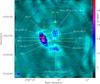 |
Fig. 1 Continuum flux image of Orion-KL at ~1.3 mm, from an assemblage of channels free of line emission. The contours are every 100 mJy/beam (uncorrected for primary beam coupling). The ten sources analyzed in detail in this work are indicated and labeled (other labels of the same sources can be found in SIMBAD/CDS): HC = hot core, CR = compact ridge, MFxx from Favre et al. (2011a), Cxx from Friedel & Weaver (2011), IRcxx from Rieke et al. (1973), Shuping et al. (2004), mmxx from Feng et al. (2015) and references therein. The yellow cross indicates the center of explosion from which the BN, I, and n sources (marked by yellow stars) are moving away (Gómez et al. 2005). The blue circles mark the primary beam coupling efficiency (though the size changes by ±8% with frequency, decreasing with increasing frequency, we keep the same median case for all the figures). The primary beam coupling correction is not applied in the present and following figures. |
Because we currently lack the zero-spacing data to recover the extended emission of many species, we generally have not attempted to derive column densities and excitation temperatures of the species we discuss here. This will be done in a future work once these data are obtained and included in the data processing. However, we tried to fit the emission with the supposition of local thermodynamical equilibrium (LTE), for all species by adjusting their column density, excitation temperature, velocity and linewidth (except for methyl cyanide, CH3CN, see Sect. 4.3). The fit was adjusted by eye to reasonably fit most of the lines of each species; this is considered a definitive determination of the line velocity and width, but not of the species column density and excitation temperature. This permits a determination of the number of velocity components necessary to fit the profiles. The LTE fit was performed using LINEDB and WEEDS sets of routines inside CLASS (Maret et al. 2011). The line catalogues are the Cologne Database for Molecular Spectroscopy (CDMS, Müller et al. 2001, 2005) and the Jet Propulsion Laboratory (JPL) catalogue (Pickett et al. 1998), with some complementary data provided by A. Belloche from the Belloche et al. (2013, hereafter B13) work to identify vibrationally excited states of vinyl and ethyl cyanides which we do not discuss in this paper but which were needed since a number of these transitions are very strong, up to 30 K.
3.1. Continuum map
Owing to the density of lines, it is somewhat difficult to find enough channels free of emission to build a continuum map. We could find two reasonably clean frequency ranges in the 218 and 235 GHz bands (bands 4 and 11 resp.), each constituting a selection of channels across the 1 GHz bandpass, which gave similar results, confirming that the channels were not polluted by line emission. Figure 1 shows the resulting continuum emission map together with the positions of the ten sources we are studying in detail in this work along with the three runaway sources (BN, I, and n), and the methyl formate peak 6 (MF6). The continuum emission (at the HC position) has a peak value of ~1.2 Jy/beam after correcting for primary beam coupling, which corresponds to a brightness of ~2.9 × 10⁴MJy/sr.
3.2. Line emission
Orion-KL molecular components.
Several molecular components, that can be distinguished both spatially and spectroscopically, are associated with Orion-KL. The hot core, compact ridge, extended ridge and plateau have been described in a number of papers (e.g. Mangum et al. 1990; Lerate et al. 2008; Friedel & Weaver 2011). A sketch illustrating the position of these components in the plane of sky is given by Irvine et al. (1987). In addition, interferometric studies of complex organic molecules have revealed the presence of other molecular clumps within Orion-KL (see e.g. Friedel & Snyder 2008; Favre et al. 2011a,b; Friedel & Widicus Weaver 2012; Brouillet et al. 2013; Peng et al. 2013). Table 2 lists the main physical parameters of the molecular components.We have extracted spectra for ten sources labeled in Fig. 1, converted them to an antenna (main beam) temperature scale using the conversion factor listed in Table 1, corrected them for beam coupling by measuring the primary beam coupling at the source position (Fig. 1), and removed any residual continuum offset (typically 0.2–0.5 K, maximum 2 K). Hereafter, bands will be called by their number, for example band 1 for the 215 150 to 216 087 MHz band, which was spectral window #3 in the first group of observations (=spw3/sg1, see Table 1). Nine sources are infrared compact sources and sometimes methyl formate (MF) sources (Favre et al. 2011a). One source, not known as an infrared peak or a MF peak but situated between the MF2 and MF6 peaks has been named the ethylene glycol peak (hereafter Et. Glycol in the figures or EGP in the text), following the discovery of aGg′ ethylene glycol ((CH2OH)2) in this location (Brouillet et al. 2015). We did not analyze MF6 because a quick inspection showed that apart from the SiO maser centered on source I and overlapping with HC, there is little difference in the main line shapes and ratios between MF6 and HC.
We have examined our data for the presence of over 130 candidate species (where a species corresponds to one entry in the JPL (Pickett et al. 1998) or CDMS (Müller et al. 2005) catalogues, which differentiate vibrationally excited states, isotopologues, isomers and conformers, representing ~60 different species and ~70 if we differentiate the isomers and conformers). Of the ~130 candidates, ~90 species are securely identified, 11 species are tentatively detected, and ~35 species already known in other sources are not detected (the list of species is presented in Table B.1). Two species, the dioxygen 18O isotopologue (16O18O) and hydroxylamine (NH2OH), have been actively searched for in the interstellar medium, but have still not been detected.
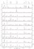 |
Fig. 2 Spectra from the band 1 setup for all ten sources. The red line indicates the 0 K (continuum-removed) level. |
 |
Fig. 3 Spectra from the band 1 setup for all ten sources with a fixed maximum temperature scale of 5 K to highlight the weaker lines. The red line indicates the 0 K (continuum-removed) level. |
Figure 2 displays the ensemble of the collected spectra for all ten sources in band 1, while Fig. 3 displays the same data expanding the vertical axis to show emission below 5 K to highlight the weaker lines. All 16 bands are presented in Appendix A, Figs. A.1–A.16, and A.17–A.32. The same data plus the combination of the fits to individual species is subsequently displayed in the same appendix in order to give an idea of the unknown lines that remain (Figs. A.33–A.48 and A.49–A.64). It is interesting to see that due to the absence of beam dilution for all sources, a large number of lines are stronger than 5 K, unlike in reported surveys from the 30 m and other single-dish telescopes (e.g. Tercero et al. 2010). Depending on the source, 13 to 29% of the channels are above 5 K, and this is only a lower limit since the intensity of lines that are produced by spatially extended emission is reduced by the lack of zero-spacing data. For the strongest lines this is clearly seen in their distorted line shape, including strongly negative channels (see, e.g., the SO line at 215 220.653 MHz in Fig. 2) and what it would be from an estimated fit (Fig. A.33).
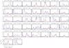 |
Fig. 4 Detection of n-C3H7CN propyl cyanide isomer towards IRc21 (see map Fig. 1). In this and the following figures, the most intense lines are displayed (i.e. lines typically stronger than ~5σ. Weaker lines are hardly or not at all detectable and have no impact on the results, nor do lines blended with much stronger lines of other species). The data are in black and the fit is in red. The summation of the fit of all the species we have identified is displayed in blue. |
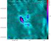 |
Fig. 6 Integrated intensity map of the 236.990 GHz set of the n-C3H7CN isomer transitions (white contours) superimposed on the continuum map. The emission toward IRc7 and IRc21 and part of the emission toward MF2 are due to this species. Emission in other regions, especially the relatively strong emission seen toward CR/MF1 is due to emission from other molecular species at different velocities and appearing at the same frequency. |
3.3. Detection of new species and new vibrationally excited states in Orion
We report the first detection in Orion of gGg′ ethylene glycol isomer ((CH2OH)2) and of acetic acid (CH3COOH), which will be presented elsewhere (Favre et al. 2017). We have also detected for the first time in Orion, n- and i-propyl cyanide conformers (C3H7CN). A few cyanoacetylene (HC3N) vibrationally excited transitions are also (probably) detected here for the first time, both for the main isotopologue and for the three singly 13C substituted isotopologues (some of them have been reported in Esplugues et al. 2013, and a contemporary paper published after the submission of the present paper also presents a study of some of these vibrationally excited states; Peng et al. 2017). Except for the gGg′ ethylene glycol isomer, only detected towards IRAS16293 A/B (Jørgensen et al. 2016), all the species we present here have been seen in some other massive star forming regions, especially in Sgr B2 (B13 discuss all of these detections concerned with Sgr B2 though some predate that work).
3.3.1. Propyl cyanide C3H7CN
Both n- and i-propyl cyanide isomer are detected (spectroscopic data are provided by Demaison & Dreizler 1982; Vormann & Dreizler 1988; Wlodarczak et al. 1988, for the n isomer and by Müller et al. 2011, for the i isomer). We mainly detect them towards IRc7, IRc21, MF2, and MF10, with a tentative detection of the n isomer towards EGP (Figs. 4 and b). Since the spatial extent of these two species is limited, we can estimate a first-order LTE column density for a given temperature. Towards the IRc21 peak, we find a column density of 1 × 1015 cm-2 for a temperature of 160 K for the n isomer and half that value for the i isomer. This n/i ratio is similar to what Belloche et al. (2014) find towards Sgr B2. However, this is not the case for MF10 (ratio of 3) nor for MF2 (ratio of 6). The column density of the n structural isomer is too small towards IRc7 to be able to detect the weaker i isomer. The variation of this n/i ratio from 2 to 6 is compatible with the modeling proposed by Garrod et al. (2017) for the medium and fast warm-up timescales of the ices in which the propyl cyanide was produced, supposing a high activation energy for reactions of CN with double-bonded hydrocarbons. Therefore, it may be a hint to how the origins of these species relate to the environment as the different clumps were and are likely exposed to a differential heating both before and after the 500-year-old explosion.
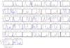 |
Fig. 7 CR/MF1 display of expected n-C3H7CN components. Despite the coincidental emission peak towards CR/MF1 in Fig. 6 that is visible in the 236.99 GHz window, n-C3H7CN is not detected in this source at a similar level to that seen in IRc21 (Fig. 4). Color-coding and TMB scale as in Fig. 4. |
In the case of such relatively rare species, blending with other species in different portions of the region is unavoidable, and therefore an intensity map of the species emission would be misleading. Figure 6 shows the integrated line intensity contour map of the seemingly isolated 236.990 GHz transition (Fig. 4) superimposed on the continuum map of the region. While C3H7CN seems to clearly peak on MF2, the real peak is towards IRc21. The MF2 peak presents a mixture of an unidentified line with propyl cyanide at that frequency. The second strongest peak, towards CR/MF1 is purely coincidental and does not represent this species, as the unsuccessful fit attempt shows (Fig. 7). This problem is general and great care should be taken when examining intensity maps of species in Orion. Identification of a species based on a single component in one of the studied sources, even if the species is clearly identified somewhere else in the region, must therefore remain very tentative.
3.3.2. Vibrationally excited HC3N and 13C singly substituted cyanoacetylene isotopologues
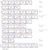 |
Fig. 8 Cyanoacetylene (HC3N) vibrationally excited transitions towards the HC. The fits help to trace the components, but have limited physical significance because their temperature is not constrained. The ν7 = 1 line at 218.861 or 237.093 GHz displays a shoulder due to the ν6 = 1 at 218.854 and 237.086 GHz, respectively). Color-coding as in Fig. 4. |
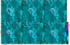 |
Fig. 9 Integrated line intensity of cyanoacetylene vibrational modes (from ν= 0 to ν6 = ν7 = 1 (white contours) superimposed on the continuum image of the region). In the ν6 = ν7 = 1 image, contours towards CR/MF1, MF2, MF4, MF5, and MF12 are not related to HC3N. |
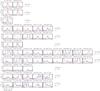 |
Fig. 10 Singly 13C substituted cyanoacetylene isotopologue lines in fundamental and first vibrationally excited modes towards IRc21. The H13CCCN ν6 = 1 mode has no transition in our bands. Color-coding as in Fig. 4. |
After the early work by Goldsmith et al. (1982, 1983), who detected the first two vibrationally excited states of cyanoacetylene (HC3N, ν7 = 1, 2), there were a few further attempts to identify higher excitation levels in this source, and finally the large work of Esplugues et al. (2013), which combines IRAM 30 m and Herschel HIFI data, reported numerous excited states (up to ν6 = ν7 = 1). It can also be noted that vibrationallyexcited states of numerous other species are now known (e.g. Daly et al. 2013; López et al. 2014). Turner (1991) invokes the HC3N ν6 = 1 transition in his analysis of a 3 mm NRAO survey, but all the transitions are always mixed with ν7 = 1 lines and are not detected separately. Since the ν7 = 1 lines are much stronger, the actual identification of the ν6 = 1 mode was not secure. de Vicente et al. (2002) report the detection of ν5 = 1, ν6 = 1, and ν7 = 1. They claim to have detected all these excited states, but show no data for ν6 = 1. Simultaneously with and independently from this work, Peng et al. (2017) published a study based on the SV0 data on part of the vibrationally excited states we report here. We note that in their study they present the ν5 = 1 and ν7 = 3 data separately, while the CDMS present them together, which is the recommended way to proceed since the states are coupled (Fermi coupling, HSP Müller, priv. comm.).
We have detected several vibrationally excited states of HC3N throughout the region and also the three 13C singly substituted isotopologues, H13CCCN, HC13CCN, and HCC13CN. Spectroscopic data are taken from Thorwirth et al. (2000), which is the most recent published measurement for HC3N, and from Thorwirth et al. (2001) for the 13C isotopologues. The highest energy vibrationally excited state we can report with confidence is the ν6 = ν7 = 1 state, at Eup≈ 1170 K and the emission is located near the HC. These are the same states as reported by Esplugues et al. (2013) from their single-dish survey. The next states, in the range 1400–1600 K, (ν7 = 4/ν7 = ν5 = 1, ν4 = 1, and ν6 = 2) are possibly seen but not securely detected3 (Fig. 8). Other excited states are reported from Sgr B2 observations in B13 but were not found in our data. Since the vibrationally excited modes are probably pumped by IR radiation, we did not try to evaluate the column density for any of these states since their temperature is not physically related to the local gas temperature. Furthermore, their excitation temperature within each vibrational state involves transitions with upper levels too close in energy to allow a secure rotational diagram analysis to be performed. As previously noted by several authors (e.g. Feng et al. 2015; Peng et al. 2017), these excited modes are mostly situated in the northern part of the region (Fig. 9). Indeed, though the ν7 = 1 and 2 states are detected even towards the CR in the southern part of the region, the higher states are only detected farther north. The excited state emission is mostly concentrated in an arc around the explosion center (Fig. 9). If they are related, it would be via collisional excitation rather than infrared pumping but all species emitting in the same arc do not seem to show the same high excitation level. We discuss the possible impact of the 500-year-old explosion in Sect. 4.4 and in a future paper on the different behavior of cyanide- and oxygen-bearing complex organic molecules in Orion-KL (Pagani et al., in prep.).
We have also detected the 13C singly substituted cyanoacetylene isotopologues in the vibrational states ν7 = 1 and 2. The next vibrational level (ν6 = 1) is most probably present, but all lines are weak and often blended (the H13CCCN ν6 = 1 vibrational state has no transitions in our bands). Towards IRc21 (named HC-North in Peng et al. 2017), the lines are stronger and less blended than towards HC and give better results (Fig. 10).
3.4. Tentative detection of new species in Orion
A number of species, already known in the interstellar medium but not detected in Orion to the best of our knowledge, have been tentatively detected in this survey. Caution should be exercised, however. As we discuss in Sect. 3.5.1, even the detection of three lines of a species is not a clear proof of its presence, independent of their signal-to-noise ratios. We therefore report these tentative detections for the sake of completeness. The addition of zero-spacing data in the future will possibly allow a better cleaning of the spectra and we hope that some of these detections will be secured. All the basic information for these species can be found at the CDMS webpage “Molecules in Space”4.
3.4.1. Methylamine CH3NH2
Methylamine was detected early on towards Sgr B2 (Kaifu et al. 1974; Fourikis et al. 1974). The same papers report its detection in Orion, but Johansson et al. (1984) proved these detections to be incorrect5. To the best of our knowledge, this species has not been reported in Orion since these early works. The line remains difficult to identify, but towards the hot core, a tentative detection can be reported thanks to several lines fitting the expected emission (Fig. 11, spectroscopic data are provided by Motiyenko et al. 2014). Possible detections are also found towards IRc7, MF2, MF5, and MF10. Towards the HC, for Tex = 280 K, we find a column density of 1 × 1016 cm-2.
3.4.2. Cyanamide NH2CN
This species has been tentatively detected by López et al. (2014). Our detection confirms their work (still tentatively), but the signal seems to come primarily from the EGP rather than from the HC (which López et al. 2014, could not distinguish in their single-dish data), 2′′ farther north, and at a velocity of 8 km s-1 instead of 5 (Fig. 12). Towards the EGP, the fit indicates a column density of 1.1 × 1014 cm-2 for Tex = 140 K. Spectroscopic data are provided by Johnson et al. (1976), Moruzzi et al. (1998).
3.4.3. Glycolaldehyde CH2(OH)CHO
Of the three C2H4O2 isomers, glycolaldehyde, acetic acid, and methyl formate, only the last is widely spread in molecular clouds and already known in Orion. Our detection of glycolaldehyde is somewhat uncertain because many lines are blended and we conservatively declare the detection to be tentative (Fig. 13). Though the fitting parameters are equivalent towards the glycol peak and MF2, the blending is slightly less severe towards MF2, which we display here. Spectroscopic data are provided by Butler et al. (2001).
3.4.4. 13C doubly substituted cyanoacetylene isotopologues
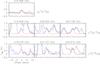 |
Fig. 14 Tentative detection of the 13C doubly substituted cyanoacetylene isotopologue lines towards IRc21. Color-coding as in Fig. 4. |
The 13C doubly substituted cyanoacetylene isotopologues have still only been tentatively detected in CRL618 (Pardo & Cernicharo 2007) and Sgr B2 (Belloche et al. 2016). Again, in Orion, the three 13C doubly substituted cyanoacetylene isotopologues are possibly detected towards IRc21 in the fundamental vibrational state (Fig. 14). The abundance ratio, in the ground vibrational state, between singly (averaged over the three isotopologues) and doubly substituted isotopologues is ~45, but because of blending, this value is likely underestimated but consistent with previous reports (Pardo & Cernicharo 2007; Belloche et al. 2016). Spectroscopic data are provided by Thorwirth et al. (2001).
3.4.5. 13C substituted Iminomethylium, H13CNH+
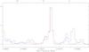 |
Fig. 15 Possible H13CNH+ line towards CR/MF1. The line is present at both LSR velocities (axis above figure) for this source. |
To the best of our knowledge, iminomethylium (HCNH+) has not yet been reported in Orion. This cation has no transition in our frequency coverage. Its (J: 3–2) line, where J is the rotational quantum number (representing the total angular momentum excluding nuclear spin), is at 222.329 GHz. Its presence must be verified in the reduced SV0 data as soon as they become available. The 13C substituted isotopologue, H13CNH+ is observed in a single transition within the frequency range covered, and is identified towards all sources, being the strongest towards CR/MF1 (Fig. 15). With only one line observed, it can at best be a tentative detection, since the density of unknown lines above 10 K is ~3.8 GHz-1 towards CR/MF1. It is only ~3 K in MF2 and is weak everywhere else (0.5–1.0 K). If confirmed, the higher abundance of iminomethylium in the richest source in oxygen-carrier complex organic molecules (hereafter O-COMs) is an interesting chemical problem, which is beyond the scope of this paper. Spectroscopy data are provided by Amano & Tanaka (1986).
3.4.6. Propanal CH3CH2CHO, propenal CH2CHCHO, and propynal CHCCHO
The three aldehydes derived from propane, propene and propyne have never been observed in Orion. Their large number of transitions and weak emission due to a relatively low abundance in this source make them difficult to detect, especially when the zero-spacing data is missing, producing negative features that can erase weak signals at the limit of sensitivity of the observations. We possibly detect propanal (spectroscopic data are provided by Hardy et al. 1982; Demaison et al. 1987) and propenal (spectroscopic data are provided by Daly et al. 2015) towards IRc21 (Figs. 16 and 17) and very tentatively propynal (spectroscopic data are provided by Winnewisser 1973; McKellar et al. 2008; Barros et al. 2015) towards the EGP (Fig. 18). Concerning propenal, three or possibly four very weak lines at the 3–5σ level are not seen out of the strongest 23 lines we report (all remaining lines not presented here are too weak to be detectable in our data). We consider that these non-detections are not significant. Propynal is not seen towards the same source because all propynal lines are weak and blended except the possible pair we present here. The 217.437 propynal transition is somewhat displaced compared to the observed peak and therefore possibly not real. The frequency displacement (1.5 MHz) is larger than the uncertainty on the transition frequency (59 kHz) even when combined with the 0.2–0.3 km s-1 fluctuation we often encounter in the fitting process. Since we present only two lines for this species, this must remain a highly tentative identification.
3.5. Non-confirmation of species in Orion
In two recent papers (Feng et al. 2015; Liseau & Larsson 2015) a tentative detection of three species has been reported. We do not confirm these detections, as discussed below.
3.5.1. Hexatriynyl C6H
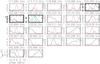 |
Fig. 19 Observations of hexatriynyl (C6H) towards SMA1 following the Feng et al. (2015) tentative detection. The three lines presented by Feng et al. (2015) are marked by thick boxes. Data are in black, the C6H model following the Feng et al. (2015) parameters in red, and its combination with vinyl cyanide at 230.108 GHz in cyan. |
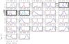 |
Fig. 20 Observations of hexatriynyl (C6H) towards the HC. The three lines presented by Feng et al. (2015) are marked by thick boxes. Data are in black, C6H modeling in red, and other species modeled in blue. The combination of C6H and vinyl cyanide emission at 230.109 GHz is shown in cyan. |
Feng et al. (2015) report the tentative detection of hexatriynyl, C6H, a precursor of the C6H− anion. They indicate that the only unblended line in their survey appears at 230.109 GHz towards their SMA1 source, 0.̋5 away from MF6 westward, though their Fig. A2 shows equally unblended lines at 220.355 and 220.487 GHz, which they fit. We find that the 230.109 GHz line is partly explained by a vibrationally excited vinyl cyanide component (C2H3CN, ν11 = 1) at 230.106 GHz, which only contributes to half of the observed line in width.
Though C6H emission could still be present (but blended with vinyl cyanide on one side and some unknown species on the other side) in this frequency window, 7 of the 21 other predicted lines (spectroscopic data are provided by Linnartz et al. 1999) falling in our survey range are not detected at all, a few others are already explained by more common species, and a few more are severely blended (Fig. 19). To better identify the possible contributors, we have also checked the C6H emission in the direction of the nearby HC (1.̋1 northeast of SMA1), see Fig. 20. There is less confusion in this direction than towards SMA1 and even more lines appear to be in disagreement. The handful of lines that could be partly explained by the C6H emission (at 217.7, 232.9, 235.8, and 250.8 GHz) are always much weaker than the prediction we make in order to fit the 231.1 GHz line. Other lines are readily explained without C6H. In particular, the 219.086 GHz line is due to a combination of vibrationally excited vinyl cyanide (C2H3CN, ν15 = 1) and vibrationally excited cyanoacetylene (HC3N, ν7 = 4/ν7 = v5 = 1 ) lines at 219.085 and 219.086 GHz, respectively; the 220.355 GHz line is due to an acetone (CH3COCH3) transition at the same frequency; and the 220.487 GHz line is due to a 13C substituted methyl cyanide (CH313CN) transition at 220.486 GHz. Since all C6H lines have comparable Einstein coefficients and since their Eup levels fall in a relatively narrow and high range of temperatures (415–550 K), it seems difficult to explain the 230.109 GHz feature as C6H while avoiding having other lines appear at some of the other frequencies. We therefore do not confirm the detection of C6H.
3.5.2. Cyanohexatriyne HC7N
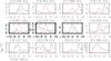 |
Fig. 21 Observations towards the HC7N peak found by Feng et al. (2015) of the 12 cyanohexatryine (HC7N) transitions recorded in our survey. Three of the four lines presented by Feng et al. (2015) are marked by thick boxes (the last one is missing from our survey). Data are in black, HC7N model following the Feng et al. (2015) parameters in red. |
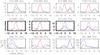 |
Fig. 22 Observations towards the HC of the 12 cyanohexatryine (HC7N) transitions recorded in our survey. Three of the four lines within the Feng et al. (2015) survey are marked by thick boxes. Data are in black, HC7N model following the Feng et al. (2015) parameters in red, other species modeling in blue. |
Feng et al. (2015) also report the tentative detection of cyanohexatriyne, HC7N, north of the HC. From their Fig. 5, the peak is approximately 2′′ due north of HC. This is close to IRc2/MF10, but 1.̋2 to the west. Though the reported lines have an Eup ≥ 1000 K, which would limit their detectability to the hottest region in Orion-KL (namely the HC), it should be noted that the vibrationally excited cyanoacetylene lines with equivalent Eup of ~1000 K are equally strong from the HC to IRc2/MF10. However, the emission area of HC7N in their Fig. 5 is not strictly coincident with this region.
Two of the four transitions in their survey range are detected and are unblended. These are the J: 196→195 and J: 205→204 transitions at 220.967 and 231.102 GHz, respectively, but they do not detect the J: 195→194 and J: 204→203 transitions at 219.841 and 229.976 GHz. This species has been possibly detected by Turner (1991) at a very low level together with HC5N, which we do not detect either (Sect. 3.7.4).
The J: 196→195 transition is outside our survey coverage, but we observed a total of 12 transitions (spectroscopic data are provided by Kirby et al. 1980; McCarthy et al. 2000; Bizzocchi & Degli Esposti 2004) including the three other transitions discussed by Feng et al. (2015). We adopt the Feng et al. (2015) parameters to compute the LTE line intensity (Tex = 155 K, N = 1 × 1016 cm-2, δv = 5 km s-1)and compare it to our data towards the emission peak of their map (Fig. 21). We do not find the same line shapes probably because our beam is much smaller and we are missing the zero-spacing data. Again, we have looked at the nearby HC region (Fig. 22) where we can run our full spectral model. Here we have increased the temperature to 200 K, which is probably the minimum temperature towards the HC, to better fit the observations, in particular the 231.1 and the 235.6 GHz lines. Six lines are completely absent and the other lines are already explained by other species. In particular, the 215.3 GHz line is due to vibrationally excited ethyl cyanide (C2H5CN, ν20 = 1), the 231.1 GHz line is due to vibrationally excited vinyl cyanide (C2H3CN, ν11 = 1), the 235.6 GHz line is due to acetone (CH3COCH3), and the 250.2 GHz line is due to a 13C substituted ethyl cyanide (C2H513CN) transition. The detection of HC7N is therefore not confirmed.
3.5.3. Hydrogen peroxide H2O2
Liseau & Larsson (2015) suggested that hydrogen peroxide (H2O2) could be present in the region because of the presence of molecular oxygen, in a similar manner to their work in the ρ Oph region. However they consider this detection to be tentative. Their peak emission position at RAJ2000 05h35m137, DecJ2000−05°22′27′′ is situated at (−6.̋8, +4.̋5) from the center of our map, i.e., about 6′′ west of MF5. Apart from the very extended emission of species like CO, CH3OH, SO, SO2, etc. there is no emission visible in this region with ALMA. However, the H2O2 line at 219.167 GHz is detected on the edge of a vibrationally excited cyanoacetylene line (HC3N, ν7 = 1, mistakenly written ν7 = 3 in their Fig. 1). This can only come from the central part of the Orion – KL region (see Sect. 3.3.2 and Fig. 8), which means that the beam is large enough to detect at least the emission of the ν7 = 1 line from the MF4/5 region. It is therefore difficult to locate the exact origin of the small signal they detected. Without the zero-spacing data, we cannot study the extended part of the region, but as far as the core is concerned, the line is not detected in the central parts of the Orion-KL region. Our survey also included the JKaKc:615→505 line at 251.915 GHz – where Ka (resp. Kc) is the projection of N onto the a (resp. c) inertial axis of the asymmetric top, and N is the rotational angular momentum quantum number, excluding electron and nuclear spin – and the JKaKc:423→515 line at 235.956 GHz, which were also not detected (spectroscopic data are provided by Bergman et al. 2011; extracted from Pickett et al. 1998).
3.6. Confirmation of formic acid HCOOH in Orion
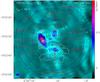 |
Fig. 24 Integrated intensity map of formic acid (HCOOH) emission at 220.038 GHz (white contours) superimposed on the continuum emission map. The main emission peaks are centered on IRc21 (compact emission) and on the EGP (Et. glycol) with an extension outside of the region. |
Feng et al. (2015) did not detect formic acid in their survey and concluded that the line is only present in extended emission since this species is known from single-dish surveys (e.g. Sutton et al. 1985). This is in contradiction with the observations of this species obtained with the Berkeley-Illinois-Maryland Association Array (BIMA) and reported by Liu et al. (2002). We confirm the detection of this species in several places (spectroscopic data are provided by Winnewisser et al. 2002), some of which were not seen in Liu et al. (2002), for example, IRc21 (Fig. 23). Figure 24 shows strong emission of limited extent centered on IRc21, and weak emission between MF4 and MF5 and between MF12 and CR/MF1. More extended emission centered on the EGP and expanding away from the explosion center seems to dominate the map. The emission being partly extended in the southern part of the Orion-KL region, the line profile towards the HC and other places seems to suffer from extended emission loss; therefore, the map should be used with caution since part of the flux is missing. The extended emission from the EGP, if real in its shape and extent, is remarkable because it points away from the explosion center. As we propose in Sect. 4.4, this could be linked to accelerated gas coming from the explosion and dragging material along from the dense and hot ridge.
3.7. Non-detection of species in Orion
There is in principle no interest in discussing lines that have not been detected in a source because this represents the vast majority of the molecules we know on Earth. But owing to the high sensitivity of this survey, one could have hoped to detect some of those species already known elsewhere in the interstellar medium, in comets, or mysteriously absent such as the first two we discuss now.
3.7.1. Dioxygen 18O isotopologue 16O18O
During a dedicated Key Program of the Herschel Space Observatory aimed at finding O2 in the interstellar medium, after the numerous negative results from SWAS (Goldsmith et al. 2000) and Odin (Pagani et al. 2003) spacecrafts, counterbalanced by a single detection in ρ Ophiuchi (Larsson et al. 2007) with Odin, we detected O2 towards Orion (Goldsmith et al. 2011) and confirmed the detection towards ρ Ophiuchi, (Liseau et al. 2012). However, the location of the emission in Orion is ill-defined and that made the interpretation of the observations difficult (Goldsmith et al. 2011; Chen et al. 2014; Melnick & Kaufman 2015). This is despite the rare velocity value of 11.3 km s-1, which should have limited the probable emission region to a few spots at the same LSR velocity as traced by the NH3 (6, 6) inversion transition (Goddi et al. 2011). In the hope of better localizing the emission region, we observed with ALMA both the Orion-KL region and the H2 vibrational peak farther north in coincidence with the Herschel pointings (Goldsmith et al. 2011; Chen et al. 2014) to try to detect the 16O18O NJ: 21 → 01 transition at 233.946 GHz. This species has never been found despite numerous attempts (e.g. Goldsmith et al. 1985; Maréchal et al. 1997a; Liseau et al. 2010). From the Herschel observations of the main isotopologue, the line was expected to be very weak (10 mJy/beam in a 5′′ source) and only ALMA could reach the needed sensitivity (2 mJy/beam) in a reasonable amount of time (from Cycle 2 onwards, with at least 37 antennas used during the observations). From the Sutton et al. (1985) survey, the frequency region in the 234 GHz band seemed clear of any strong emission and the prospect of finding 16O18O looked reasonable.
16O18O can be searched from the ground because the species is not homonuclear and therefore, in contrast to 16O2, both even and odd rotational quantum numbers N are allowed, giving permitted transitions between levels which do not exist for 16O2. These transitions occur at frequencies totally free of 16O2 emission and are therefore unblocked by the atmosphere except in a narrow range (±10 MHz) around the rest frequency of the line, which can usually be avoided as a consequence of the Fizeau-Doppler shift resulting from the Earth’s orbital velocity around the Sun. The line predicted to be the strongest in the interstellar medium is the NJ: 21→01 at 234 GHz (Maréchal et al. 1997b) that has been actively searched for from 1985 up to the end of the 1990s when satellites equipped with heterodyne receivers started to look directly for the main species 16O2, 250 times more abundant, but still without success (see Goldsmith et al. 2011, for a review). The discovery of 16O2 in ρ Oph (Larsson et al. 2007) triggered a last, still unsuccessful attempt to find 16O18O in that source (Liseau et al. 2010). Owing to the relatively rare LSR velocity of the O2 emission (VLSR = 11.3 km s-1) in this source, we thought that the emitting region could only be one of the small regions in that velocity range revealed by NH3(6, 6) emission (Goddi et al. 2011), namely the MF4/MF5 region, which is the main region emitting in the 11 km s-1 range. However, we unexpectedly found a pair of vibrationally excited lines of ethyl cyanide (C2H5CN, ν13 = 1/ν21 = 1) at 233.945 GHz emitting a signal strong enough to completely mask the weak signal that we were expecting (~150–200 mK, Fig. 25) from our 16O2 detection (Goldsmith et al. 2011; Chen et al. 2014). Therefore, the expected presence of molecular oxygen in the Orion-KL region cannot be evaluated since the fitting of the ethyl cyanide line will never be secure enough to quantify any residual emission (this does not include the position farther to the north discussed in Chen et al. 2014; and Melnick & Kaufman 2015, which we postpone to a future paper).
3.7.2. Hydroxylamine NH2OH
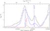 |
Fig. 25 16O18O observations towards MF4. The expected line is traced in red together with the data (black) and LTE modeling of other species (blue). The parameters for these species have been adjusted from other components and do not exactly match the present lines because of the simplicity of the LTE model. |
This species has never been identified in space, though it is predicted by chemical models (Pulliam et al. 2012; McGuire et al. 2015). In our bands, the only strong and likely observable lines are in the range 251.7–252.0 GHz (J: 5→4, Eup = 36–164 K, spectroscopic data are provided by Tsunekawa 1972; Morino et al. 2000), a region which is densely packed with many strong methanol lines plus the SO NJ: 65→54 transition at 251.825 GHz, which all suffer from the absence of zero-spacing data, making their modeling impossible. Among the nine lines in this range, only one pair of lines is not blended with methanol, SO and ethyl cyanide strong emissions. These are the two JKaKc: 533→432 and JKaKc: 532→431 lines at 251.780 GHz with Eup = 107.8 K. It is therefore impossible to search for this species, but we note that this line is possibly seen in one place in Orion-KL in order to focus some further searches at other frequencies at the same place. The spectrum shown in Fig. 26 was taken 0.̋9 west of the EGP, i.e., at RAJ2000 05h35m1444, DecJ2000−05°22′32.̋8.
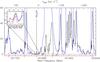 |
Fig. 26 Hydroxylamine (NH2OH) line observation 0.̋9 west of the EGP. The six red arrows mark the positions of the nine NH2OH lines (three lines are a combination of two transitions with very little or no spacing). The one possible detection is zoomed. Color-coding as in Fig. 4. |
3.7.3. Other species
We have searched without success for a number of species known in the interstellar medium but not yet identified in Orion, including propadienone (C3H2O), thiocyanic acid, (HSCN), isothiocyanic acid HNCS, cyanomethylene (HCCN), ketenyl (HCCO), cyanoamidogen (HNCN), cyanic acid (HOCN), cya noformaldehyde HCOCN, protonated carbon dioxide (HOCO+), hydroperoxyl (HO2), cyclopropanediylidenyl (c-C3H), propadienylidene (l-C3H2), cyclopropenone c-C3H2O, cyanopropyne (CH3C3N), N-protonated isocyanic acid (H2NCO+), methylene amidogen (H2CN), methyl peroxide (CH3OOH), deuterated diazenylium (N2D+), aminoacetonitrile (H2NCH2CN), and protonated cyanoacetylene (HC3NH+).
It is remarkable that despite the large abundance of isocyanic acid (HNCO) and of cyanoacetylene (HC3N), their protonated forms are not detected, though for the former we have only one line that falls within our survey and it is often blended.
3.7.4. Extended emission
A few species have not been detected in our survey, while their detection seems firmly established in previous studies carried out with single dishes (Johansson et al. 1984; Madden et al. 1989; Turner 1991; Tercero et al. 2010). We believe that their non-detection is due to their extended, smoothly distributed emission.
This is the case of cyclopropenylidene (c-C3H2) reported by Madden et al. (1989) and Turner (1991). Turner (1991) explains that this species is emitted from a cold region that is not coming from Orion-KL but from an extended region surrounding it.
We do not detect thioxoethenylidene (CCS). Turner (1991) reports a fit with Trot = 19 K. Though he does not comment on this result, it is possible to think that this low temperature argues again for extended emission, consistent with our non-detection. However Tercero et al. (2011) report the detection of both C2S and thioxopropadienylidene (C3S) with the IRAM 30 m as coming from the hot core. These cases should be resolved once existing single-dish data (zero-spacing) are added to our ALMA data.
Cyanobutadiyne (HC5N) is reported by Johansson et al. (1984), Turner (1991), and Esplugues et al. (2013). Johansson et al. (1984) mentions that its emission is extended since they found weaker emission with their smaller beam, compared to what was found in earlier investigations. If extended, it might explain why lines of HC5N were not detected in our survey, but the analysis of Esplugues et al. (2013) pin-points the emission to the outer hot core (though the position is not precisely defined in the paper) and to the CR. The column density of HC5N for the CR fit (3× 1012 cm-2) is too low for this species to emit a detectable line in our data, while the column density for the HC fit (7 × 1013 cm-2) is compatible with an emitted line of HC5N for only one out of our six unblended HC5N lines present in our survey (but not as large as 10 km s-1). Its non-detection for the other lines is compatible with a column density seven times lower at the ~3σ level.
3.7.5. Out of band species
Our survey was not continuous in frequency, and so a number of interesting species between 215 and 252 GHz were not observed. The interested reader is referred to the SV0 data to retrieve them: iminomethylium (HCNH+), propyne (CH3CCH), carbonyl sulfide isotopologues (OC33S, OC34S), ethynyl (CCH) and its 13C substituted isotopologues (but CCD is observed though not detected), propynylidyne (l-C3H), deuterated formyl (DCO+), deuterated isocyanide (DNC), phosphorus nitride (PN), nitrogen sulfide (NS), the other 13C substituted methyl cyanide isotopologue (13CH3CN), and fulminic acid (HCNO). Some species were present only in blends with stronger lines like the 13C substituted thioformyl (H13CS+) cation.
4. Discussion: velocity structure of the source
The velocity structure of Orion-KL is complex. The NH3(6, 6) velocity map of Goddi et al. (2011) reveals (as do other studies) many velocity components, and in our survey some species have complex structure with numerous velocity components ranging from −15 to 25 km s-1, that are emitted from both the extended region and from the compact core. However, because of the lack of short spacings, there is some confusion regarding the velocity structure for the molecules with extended emission. Therefore, we focus on the emission from molecules that arise only from the small dense and hot components of the region where the lack of short spacings should not be a problem. Even these components show a complex velocity (Sect. 4.1). We also show that some velocity components on the same line of sight can be ordered (Sect. 4.3) and that the 500-year-old explosion could have an impact on the region around it that is observable in the line profiles (Sect. 4.4).
4.1. Kinematic complexity
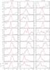 |
Fig. 27 Methanol (CH3OH), vinyl cyanide (C2H3CN), and ethyl cyanide (C2H5CN) line profiles for the ten sources (see Fig. 1). The black line traces the data and the red line the LTE fit. The vertical dashed lines represent the velocity components introduced in the fit to match the observations. |
 |
Fig. 28 Velocities of the main components towards the ten sources in our study superimposed on a copy of Fig. 1. The alternating white and black arrows and figures have no meaning and are only used to separate more clearly the list of velocities at each spot. |
 |
Fig. 29 Line shape difference between methanol (CH3OH) and methyl formate (CH3OCHO) towards MF4 for different transitions of methanol (in black; the upper state energy (K) and the torsional mode are indicated to the right) compared to the same methyl formate line (in red) for reference. The blue line marks the 9 km s-1 average velocity of the region. |
The velocity structure of the region is extremely complex. Depending on the species, spectra toward different sources show up to four distinct components, sometimes with different species agreeing in velocity, and sometimes differing. This is obviously true for species like CO, SO, SO2, H2CO, SiO, which have emission associated with each of the ten sources, but which also have emission on larger scales and part of this emission can be lost due to the interferometer filtering of extended emission. The net effect is that this can produce velocity components that are not real. We will not address these molecules further, but will address them later when we have added the zero-spacing data. This complex velocity structure is also present in molecules whose emission is limited to the hot spots; for example, vinyl and ethyl cyanides show the largest number of velocity components often not in coincidence with O-COMs like methanol and methyl formate. Figure 27 presents the line shape of three species (methanol, vinyl and ethyl cyanides) for all ten sources. The velocity components introduced in the model are traced by the vertical dashed lines. A few of them are introduced solely to reproduce the velocity wings, although we did not always undertake fitting these wings in detail (for example the wings of the cyanide species towards IRc7 and IRc21). A typical case is the CR/MF1 spot which needs two velocity components to fit the methanol line (and all the O-COMs) and four velocity components to fit the ethyl cyanide lines. The main velocity component goes from 0 to 11.2 km s-1, with still important components beyond (down to −7 or up to +19 km s-1). The main cyanide velocity component sometimes has no corresponding emission in methanol (MF2, MF12, EGP). A first moment map of the emission of these species, like the NH3(6, 6) map invoked earlier, would not render the complexity of this situation for sources like IRc7, MF2, the EGP, etc. Instead, we have produced a map where we indicate numerically the velocity of the various components (Fig. 28). Even these velocities are only indicative of a few species. The only relatively simple cases are IRc21 with a single component (but a strong blue wing) and the HC with two velocity components, one at 4.3 km s-1 at which all the cyanides emit, and a second one between 5.4 and 5.8 km s-1 that corresponds to the O-COMs. There are a few aberrant cases such as ethanol (C2H5OH) at ~5 km s-1, doubly deuterated formaldehyde (D2CO) at 6.4 km s-1, and vibrationally excited cyanoacetylene (HC3N) ν7 = 1 components at −5.7 and 15.7 km s-1 and ν7 = 2 at −5.5 km s-1 in addition to the standard 4.3 km s-1 component. To make this picture consistent, a strongly perturbing event is required. We suggest that the kinematic structure of the molecules in this region is linked to the explosion which occurred 500 yr ago (Pagani et al., in prep.), an idea also proposed by Zapata et al. (2011).
4.2. Chemical complexity
We also find differences between methanol and methyl formate, which are supposed to be chemically linked. The most striking case is towards MF4 (Fig. 29) where for any methanol line energy level, the line shape differs notably from the methyl formate line taken as a reference. This is therefore not an excitation effect or an extended emission loss for methanol. The coincidence of the two species is therefore not systematic and this different shape reflects an ongoing chemical evolution which deserves proper attention once the zero-spacing data is added. Similarly, Tercero et al. (2015) mention a different peak position for 13CH3OH and methyl formate along the ridge centered on the HC peak which they also interpret as ongoing transformation of methanol to methyl formate.
This complexity makes the single-dish telescope searches of weak lines difficult because of the mixing of many velocity components for each species. Even with ALMA resolving the sources and separating the components, great care must be taken to analyze the lines and correctly account for all components.
Another consequence of this complexity is the difficulty in deriving abundances. The total column density is derived from the dust emission (or the CO emission if it is possible to securely separate the local emission from the general emission) which cannot be split between the different velocity components. It seems therefore difficult to derive abundances per velocity component and attention should be paid to this problem when addressing the chemical evolution of the region.
4.3. Line of sight structure
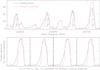 |
Fig. 30 Fit of CH3CN K components of the J: 12→11 rotational transition towards MF5. Upper panel: fit of four K ladder components. Lower level: three velocity components ordered differently on the line of sight to fit the observed profile of the K = 3 transition (scaled to visually match the observations). |
In the band 6 setup, we observed the methyl cyanide (CH3CN) ladder from JK: 123→ 113 (220.709 GHz) up to JK: 1211 → 1111 (220.235 GHz, Fig. A.6). The first transition is highly optically thick and when several velocity components are present on the same line of sight, the combination of their emission and absorption can change the observed profile if they are close enough in velocity to interact significantly. Though this low upper energy level transition is probably extended and some flux is missing, we identify such an effect towards three sources, MF4, MF5 and MF10, for which we can try to match the profile by combining the velocity components in different sequences. Figure 30 shows the fit of methyl cyanide towards MF5. Unlike for all the other species, we use a non-LTE radiative transfer code (RADEX, van der Tak et al. 2007) to compute the line intensity since the structure of the symmetric top allows us to scan a wide range of energy levels for the same J level at nearby frequencies. The collisional coefficients are taken from Green (1986). The model includes three velocity components to match most of the line (we ignored the linewing), at 6.2, 9, and 11 km s-1, similar to the velocity components we found for the other species, but slightly closer to the velocities of the O-COMs than to those of vinyl and ethyl cyanide (differences of a few tenths of km s-1). While we manage to find a solution for the K = 4–6 transitions, the modeled K = 3 transition is always stronger than the observed line, most probably due to the loss of extended emission in the observations (Fig. 30, upper panel). If we rescale the spectrum to fit the observations for the K = 3 transition, we find that out of the six possible combinations, only one solution fits the observed profile (Fig. 30, lower panel). Two solutions are not shown because they give identical results to two others: when the central velocity component is in front or behind the two extreme velocity components, permuting the two extreme velocity components which do not mutually interfere makes no difference. With the supposition that the missing zero-spacing data would not change the line shape, we have ordered the velocity components of the three sources (MF4, MF5, MF10). Table 3 presents the results. For MF4 and MF5, the redshifted components are behind and the blueshifted components are in front, which indicates an expansion of the cloudlets, i.e. the cloudlets are receding at increasing velocities with increasing distance while for MF10, the reverse situation applies and the two components at positive velocity are moving towards each other (the third component at negative velocity does not interact and cannot be positioned).
Order of velocity components along the line of sight.
4.4. Impact of the explosion on the cores
Figure 1 shows the position (yellow cross) where the 500-year-old explosion most probably took place (Gómez et al. 2005; Zapata et al. 2009). It is situated in the center of a belt of emission passing through IRc21, IRc2/MF10, HC, IRc7, IRc20/MF4 and IRc6/MF5. A number of works have revealed the H2 and the 12CO expansions linked to this explosion (e.g. Allen & Burton 1993; Zapata et al. 2009; Nissen et al. 2012; Youngblood et al. 2016) but it seems that the interaction of this event with the surrounding cores has only been considered by Zapata et al. (2011). While we will address in greater details the link we see between the explosion and a number of species peculiar velocity distributions (including nitrogen monoxide, isocyanic acid, vinyl and ethyl cyanide) in a forthcoming paper (Pagani et al., in prep.), we want to mention a number of facts of interest here.
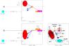 |
Fig. 31 Different components in the KL region following the discussion in Sects. 4.4 and 4.5. The front view shows the continuum contours from Fig. 1 employing simple elliptical shapes to indicate the different parts of the cloud. The red ellipse includes the HC ridge, encompassing IRc21, MF10, MF6, MF2, and the glycol peak. The explosion center is indicated by the set of orange arrows, and the velocity shifts of both the bulk of the gas and the line wings are shown in the corresponding color. The respective position of MF12 (dark blue), IRc7 (green) and the HC group along the Z-axis is not known and the arrangement shown is arbitrary. The only constraint is that MF4 (purple)/MF5 (orange) be behind the explosion center and the rest of the components be in front along the Z-axis. We have also not given any inclination or bent shape to the HC ridge along the Z-axis. The CR/MF1 (cyan) source is supposed to be at least 10 000 AU in front but could also be behind. MF4 and MF5 are split into three blobs with small velocity arrows of increasing length (and possibly approaching the observer for the first MF5 blob) to illustrate that the farther away from the explosion center, the higher is the source’s velocity (see Table 3). |
We already mentioned the interesting formic acid (HCOOH) extended emission away from the explosion center in Sect. 3.6. We also note that the vibrationally excited lines of cyanoacetylene (HC3N), but also those of other species (vinyl and ethyl cyanides, which will be presented in Pagani et al., in prep.) are following the belt mentioned above (Fig. 9). Figure 27 also shows prominent wings on the methanol emission lines (and other molecules) towards sources that lie closer to the explosion center. MF4 and MF5 on the west of the explosion center display red wings, while IRc21, IRc7, and MF10, which lie southeast of the explosion center, display blue wings. Overall, the velocity components of MF4 and MF5 are all above 6 km s-1 while low or even negative components are found on the eastern side. We suggest that these wings are tracing material being accelerated by the high velocity (>100 km s-1) outflowing gas resulting from the explosion. This would indicate that MF4 and MF5 are located behind the explosion center (to explain the red wings and the 9 to 13 km s-1 velocity components) and that they are receding from it, away from us, while the HC long ridge (including sources from MF2 to MF10, and possibly IRc21) is in front of the explosion center, also moving away from it, but towards us (to explain the blue wings and the velocity components mostly between 0 and 6 km s-1). The recession of all the molecular clumps in Orion-KL is possibly induced by the slow (15 km s-1) bubble expansion, i.e., 7.5 km s-1 radial (Zapata et al. 2011), following the explosion, but this requires further investigation. The whole structure, including the discussion of the compact ridge position (Sect. 4.5), is depicted in a sketch (Fig. 31), though we currently have no information to position in detail those parts of the region that are in front of the explosion center with respect to each other, nor of the MF4 and MF5 substructures in between them and relative to the other groups.
4.5. Compact ridge
The compact ridge (CR/MF1) is very different from all the other cores. Ethyl cyanide (C2H5CN) emission is weak and vinyl cyanide (C2H3CN) is absent. It is an extremely quiescent emitter with lines close to 1 km s-1 width, sometimes barely resolved (or not at all) with our backend setup (~0.6 km s-1), as illustrated by the tentative Gaussian fit of three methyl formate (CH3OCHO) components towards this source (Fig. 32). The narrow components have line widths in the range 0.9–1.4 km s-1. The line wings are symmetrical. Only the two lowest vibrational energy levels of cyanoacetylene are populated. It seems therefore that this core has escaped (at least until the present time) the influence of the explosive event. Since the much smaller IRc4/MF12 clump just above CR/MF1 is similar to the ring fragments in terms of line shape, asymmetric wings, and excitation, and is therefore being affected by the explosive event, it seems more probable that the CR is far enough away to have not yet been reached. Examining the maximum extent of the 12CO filaments (Zapata et al.2009; 20–35′′ southward, up to 50′′ northward), we can consider that CR/MF1 has to be at least at such a distance to have escaped the high velocity gas until now. Orion’s distance of 388 pc combined with the angular offset of 50′′ corresponds to 20 000 au. Since CR/MF1 is only 10′′ south of the explosion center, it must be in front of or behind the explosion center by at least 10 000 au (for the typical 25′′ CO bullet distance southward) and more probably by 20 000 au, and is therefore only loosely related to the other Orion-KL cores. Wang et al. (2010) also indicate the existence of a cavity between the HC and the CR from their analysis of high rotation levels of methyl cyanide.
5. Conclusions
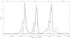 |
Fig. 32 Three methyl formate (CH3OCHO) components observed towards CR/MF1. Data are in black; individual components: narrow are in red, wide are in green, sum of the components are in blue. |
We have observed 16 GHz of bandpass in the 1.3 mm window towards Orion-KL during the ALMA Cycle 2. The angular and resulting spatial resolution are sufficient to separate all the components of the region; the spectral resolution that we have employed is also sufficient except towards the compact ridge, which presents narrow lines close to 1 km s-1 only. Numerous interesting results already emerge from this first study, demonstrating the need to analyze all the dense structures as well as all the main lines in parallel to obtain a consistent model of this complex region. A wealth of information remains to be extracted from these data; in addition to possibly revealing new molecules, this new information will also help to better understand the structure and evolution of this source.
For an energy level diagram of the vibrational states of HC3N, see Yamada & Creswell (1986).
This information has been taken from the CDMS webpage on methylamine: http://www.astro.uni-koeln.de/site/vorhersagen/molecules/ism /MeNH2.html
Acknowledgments
We thank an anonymous referee for the careful reading of the document; we enjoyed our discussion, which helped to improve the presentation of our results. We thank the IRAM ARC center for their hospitality and coaching for the ALMA data reduction process, in particular Gaëlle Dumas and Edwige Chapillon, ESO for the financial support during the visit to the ARC (MARCUs funding) and Crystal Brogan for her help and suggestions throughout the preparation and data reduction processes. This work made use of the SIMBAD resource offered by CDS Strasbourg, France, of the CDMS and JPL molecular line databases offered by the Köln University and by NASA respectively. We thank Arnaud Belloche and Holger Müller for their great help in the identification of the excited modes of cyanide species and other advice that they endlessly provided. L.P. thanks the CNRS for the permanent funding of his position, without which this work could not have been performed. A short term funding would never had permitted this type of work. C.F. acknowledges funding from the French space agency CNES, and support from the Italian Ministry of Education, Universities and Research, project SIR (RBSI14ZRHR). This work was carried out in part at the Jet Propulsion Laboratory, which is operated for NASA by the California Institute of Technology. E.A.B. acknowledges support from the National Science Foundation grant AST-1514670.
References
- Allen, D. A., & Burton, M. G. 1993, Nature, 363, 54 [NASA ADS] [CrossRef] [Google Scholar]
- Amano, T., & Tanaka, K. 1986, J. Mol. Spect., 116, 112 [NASA ADS] [CrossRef] [Google Scholar]
- Barros, J., Appadoo, D., McNaughton, D., et al. 2015, J. Mol. Spect., 307, 44 [NASA ADS] [CrossRef] [Google Scholar]
- Belloche, A., Müller, H. S. P., Menten, K. M., Schilke, P., & Comito, C. 2013, A&A, 559, A47 [NASA ADS] [CrossRef] [EDP Sciences] [Google Scholar]
- Belloche, A., Garrod, R. T., Müller, H. S. P., & Menten, K. M. 2014, Science, 345, 1584 [NASA ADS] [CrossRef] [PubMed] [Google Scholar]
- Belloche, A., Müller, H. S. P., Garrod, R. T., & Menten, K. M. 2016, A&A, 587, A91 [NASA ADS] [CrossRef] [EDP Sciences] [Google Scholar]
- Bergin, E. A., Phillips, T. G., Comito, C., et al. 2010, A&A, 521, L20 [NASA ADS] [CrossRef] [EDP Sciences] [Google Scholar]
- Bergman, P., Parise, B., Liseau, R., et al. 2011, A&A, 531, L8 [NASA ADS] [CrossRef] [EDP Sciences] [Google Scholar]
- Bizzocchi, L., & Degli Esposti, C. 2004, ApJ, 614, 518 [NASA ADS] [CrossRef] [Google Scholar]
- Blake, G. A., Sutton, E. C., Masson, C. R., & Phillips, T. G. 1986, ApJS, 60, 357 [NASA ADS] [CrossRef] [Google Scholar]
- Blake, G. A., Sutton, E. C., Masson, C. R., & Phillips, T. G. 1987, ApJ, 315, 621 [NASA ADS] [CrossRef] [Google Scholar]
- Brouillet, N., Despois, D., Baudry, A., et al. 2013, A&A, 550, A46 [NASA ADS] [CrossRef] [EDP Sciences] [Google Scholar]
- Brouillet, N., Despois, D., Lu, X. H., et al. 2015, A&A, 576, A129 [NASA ADS] [CrossRef] [EDP Sciences] [Google Scholar]
- Butler, R. A. H., De Lucia, F. C., Petkie, D. T., et al. 2001, ApJS, 134, 319 [NASA ADS] [CrossRef] [Google Scholar]
- Cernicharo, J., Kisiel, Z., Tercero, B., et al. 2016, A&A, 587, L4 [NASA ADS] [CrossRef] [EDP Sciences] [Google Scholar]
- Chen, J.-H., Goldsmith, P. F., Viti, S., et al. 2014, ApJ, 793, 111 [NASA ADS] [CrossRef] [Google Scholar]
- Crockett, N. R., Bergin, E. A., Neill, J. L., et al. 2014, ApJ, 787, 112 [NASA ADS] [CrossRef] [Google Scholar]
- Daly, A. M., Bermúdez, C., López, A., et al. 2013, ApJ, 768, 81 [NASA ADS] [CrossRef] [Google Scholar]
- Daly, A. M., Bermúdez, C., Kolesniková, L., & Alonso, J. L. 2015, ApJS, 218, 30 [NASA ADS] [CrossRef] [MathSciNet] [Google Scholar]
- de Vicente, P., Martín-Pintado, J., Neri, R., & Rodríguez-Franco, A. 2002, ApJ, 574, L163 [NASA ADS] [CrossRef] [Google Scholar]
- Demaison, J., & Dreizler, H. 1982, Zeitschrift Naturforschung Teil A, 37, 199 [NASA ADS] [CrossRef] [Google Scholar]
- Demaison, J., Maes, H., Van Eijck, B. P., Wlodarczak, G., & Lasne, M. C. 1987, J. Mol. Spect., 125, 214 [NASA ADS] [CrossRef] [Google Scholar]
- Esplugues, G. B., Cernicharo, J., Viti, S., et al. 2013, A&A, 559, A51 [NASA ADS] [CrossRef] [EDP Sciences] [Google Scholar]
- Favre, C., Despois, D., Brouillet, N., et al. 2011a, A&A, 532, A32 [NASA ADS] [CrossRef] [EDP Sciences] [Google Scholar]
- Favre, C., Wootten, H. A., Remijan, A. J., et al. 2011b, ApJ, 739, L12 [NASA ADS] [CrossRef] [Google Scholar]
- Favre, C., Pagani, L., Goldsmith, P. F., et al. 2017, A&A, 604, L2 [NASA ADS] [CrossRef] [EDP Sciences] [Google Scholar]
- Feng, S., Beuther, H., Henning, T., et al. 2015, A&A, 581, A71 [NASA ADS] [CrossRef] [EDP Sciences] [Google Scholar]
- Fourikis, N., Takagi, K., & Morimoto, M. 1974, ApJ, 191, L139 [NASA ADS] [CrossRef] [Google Scholar]
- Friedel, D. N., & Snyder, L. E. 2008, ApJ, 672, 962 [NASA ADS] [CrossRef] [Google Scholar]
- Friedel, D. N., & Weaver, S. L. W. 2011, ApJ, 742, 64 [NASA ADS] [CrossRef] [Google Scholar]
- Friedel, D. N., & Widicus Weaver, S. L. 2012, ApJS, 201, 17 [NASA ADS] [CrossRef] [Google Scholar]
- Garrod, R. T., Belloche, A., Müller, H. S. P., & Menten, K. M. 2017, A&A, 601, A48 [NASA ADS] [CrossRef] [EDP Sciences] [Google Scholar]
- Goddi, C., Greenhill, L. J., Humphreys, E. M. L., Chandler, C. J., & Matthews, L. D. 2011, ApJ, 739, L13 [NASA ADS] [CrossRef] [Google Scholar]
- Goldsmith, P. F., Snell, R. L., Deguchi, S., Krotkov, R., & Linke, R. A. 1982, ApJ, 260, 147 [NASA ADS] [CrossRef] [Google Scholar]
- Goldsmith, P. F., Krotkov, R., Snell, R. L., Brown, R. D., & Godfrey, P. 1983, ApJ, 274, 184 [NASA ADS] [CrossRef] [Google Scholar]
- Goldsmith, P. F., Snell, R. L., Erickson, N. R., et al. 1985, ApJ, 289, 613 [NASA ADS] [CrossRef] [PubMed] [Google Scholar]
- Goldsmith, P. F., Melnick, G. J., Bergin, E. A., et al. 2000, ApJ, 539, L123 [NASA ADS] [CrossRef] [Google Scholar]
- Goldsmith, P. F., Liseau, R., Bell, T. A., et al. 2011, ApJ, 737, 96 [Google Scholar]
- Gómez, L., Rodríguez, L. F., Loinard, L., et al. 2005, ApJ, 635, 1166 [NASA ADS] [CrossRef] [Google Scholar]
- Green, S. 1986, ApJ, 309, 331 [NASA ADS] [CrossRef] [Google Scholar]
- Hardy, J. A., Cox, A. P., Fliege, E., & Dreizler, H. 1982, Zeitschrift Naturforschung Teil A, 37, 1035 [NASA ADS] [CrossRef] [Google Scholar]
- Hirota, T., Kim, M. K., & Honma, M. 2012, ApJ, 757, L1 [NASA ADS] [CrossRef] [Google Scholar]
- Irvine, W. M., Goldsmith, P. F., & Hjalmarson, Å. 1987, in Interstellar processes, Proc. Symp., Five College Radio Astronomy Observatory, Amherst, MA (Dordrecht: Springer Netherlands), 561 [Google Scholar]
- Johansson, L. E. B., Andersson, C., Ellder, J., et al. 1984, A&A, 130, 227 [Google Scholar]
- Johnson, D. R., Suenram, R. D., & Lafferty, W. J. 1976, ApJ, 208, 245 [NASA ADS] [CrossRef] [Google Scholar]
- Jørgensen, J. K., van der Wiel, M., Coutens, A., et al. 2016, A&A, 595, A117 [NASA ADS] [CrossRef] [EDP Sciences] [Google Scholar]
- Kaifu, N., Morimoto, M., Nagane, K., et al. 1974, ApJ, 191, L135 [NASA ADS] [CrossRef] [Google Scholar]
- Kirby, C., Kroto, H. W., & Walton, D. R. M. 1980, J. Mol. Spectr., 83, 261 [NASA ADS] [CrossRef] [Google Scholar]
- Kounkel, M., Hartmann, L., Loinard, L., et al. 2017, ApJ, 834, 1 [Google Scholar]
- Larsson, B., Liseau, R., Pagani, L., et al. 2007, A&A, 466, 999 [Google Scholar]
- Lerate, M. R., Yates, J., Viti, S., et al. 2008, MNRAS, 387, 1660 [NASA ADS] [CrossRef] [Google Scholar]
- Linnartz, H., Motylewski, T., Vaizert, O., et al. 1999, J. Mol. Spect., 197, 1 [NASA ADS] [CrossRef] [PubMed] [Google Scholar]
- Liseau, R., & Larsson, B. 2015, A&A, 583, A53 [NASA ADS] [CrossRef] [EDP Sciences] [Google Scholar]
- Liseau, R., Larsson, B., Bergman, P., et al. 2010, A&A, 510, A98 [NASA ADS] [CrossRef] [EDP Sciences] [Google Scholar]
- Liseau, R., Goldsmith, P. F., Larsson, B., et al. 2012, A&A, 541, A73 [NASA ADS] [CrossRef] [EDP Sciences] [Google Scholar]
- Liu, S.-Y., Girart, J. M., Remijan, A., & Snyder, L. E. 2002, ApJ, 576, 255 [NASA ADS] [CrossRef] [Google Scholar]
- López, A., Tercero, B., Kisiel, Z., et al. 2014, A&A, 572, A44 [NASA ADS] [CrossRef] [EDP Sciences] [Google Scholar]
- Madden, S. C., Irvine, W. M., Swade, D. A., Matthews, H. E., & Friberg, P. 1989, AJ, 97, 1403 [NASA ADS] [CrossRef] [PubMed] [Google Scholar]
- Mangum, J. G., Wootten, A., Wadiak, E. J., & Loren, R. B. 1990, ApJ, 348, 542 [NASA ADS] [CrossRef] [Google Scholar]
- Maréchal, P., Pagani, L., Langer, W. D., & Castets, A. 1997a, A&A, 318, 252 [NASA ADS] [Google Scholar]
- Maréchal, P., Viala, Y. P., & Pagani, L. 1997b, A&A, 328, 617 [NASA ADS] [Google Scholar]
- Maret, S., Hily-Blant, P., Pety, J., Bardeau, S., & Reynier, E. 2011, A&A, 526, A47 [NASA ADS] [CrossRef] [EDP Sciences] [Google Scholar]
- McCarthy, M. C., Levine, E. S., Apponi, A. J., & Thaddeus, P. 2000, J. Mol. Spect., 203, 75 [NASA ADS] [CrossRef] [Google Scholar]
- McGuire, B. A., Carroll, P. B., Dollhopf, N. M., et al. 2015, ApJ, 812, 76 [NASA ADS] [CrossRef] [Google Scholar]
- McKellar, A. R. W., Watson, J. K. G., Chu, L.-K., & Lee, Y.-P. 2008, J. Mol. Spect., 252, 230 [NASA ADS] [CrossRef] [Google Scholar]
- McMullin, J. P., Waters, B., Schiebel, D., Young, W., & Golap, K. 2007, in Astronomical Data Analysis Software and Systems XVI, eds. R. A. Shaw, F. Hill, & D. J. Bell, ASP Conf. Ser., 376, 127 [Google Scholar]
- Melnick, G. J., & Kaufman, M. J. 2015, ApJ, 806, 1 [NASA ADS] [CrossRef] [Google Scholar]
- Menten, K. M., Reid, M. J., Forbrich, J., & Brunthaler, A. 2007, A&A, 474, 515 [NASA ADS] [CrossRef] [EDP Sciences] [Google Scholar]
- Morino, I., Yamada, K. M. T., Klein, H., et al. 2000, J. Mol. Struct., 517, 367 [NASA ADS] [CrossRef] [Google Scholar]
- Moruzzi, G., Jabs, W., Winnewisser, B. P., & Winnewisser, M. 1998, J. Mol. Spect., 190, 353 [NASA ADS] [CrossRef] [Google Scholar]
- Motiyenko, R. A., Ilyushin, V. V., Drouin, B. J., Yu, S., & Margulès, L. 2014, A&A, 563, A137 [NASA ADS] [CrossRef] [EDP Sciences] [Google Scholar]
- Müller, H. S. P., Thorwirth, S., Roth, D. A., & Winnewisser, G. 2001, A&A, 370, L49 [NASA ADS] [CrossRef] [EDP Sciences] [Google Scholar]
- Müller, H. S. P., Schlöder, F., Stutzki, J., & Winnewisser, G. 2005, J. Mol. Struct., 742, 215 [NASA ADS] [CrossRef] [Google Scholar]
- Müller, H. S. P., Coutens, A., Walters, A., Grabow, J.-U., & Schlemmer, S. 2011, J. Mol. Spect., 267, 100 [CrossRef] [Google Scholar]
- Nissen, H. D., Cunningham, N. J., Gustafsson, M., et al. 2012, A&A, 540, A119 [NASA ADS] [CrossRef] [EDP Sciences] [Google Scholar]
- Pagani, L., Olofsson, A. O. H., Bergman, P., et al. 2003, A&A, 402, L77 [NASA ADS] [CrossRef] [EDP Sciences] [Google Scholar]
- Pardo, J. R., & Cernicharo, J. 2007, ApJ, 654, 978 [NASA ADS] [CrossRef] [Google Scholar]
- Peng, T. C., Despois, D., Brouillet, N., Parise, B., & Baudry, A. 2012, A&A, 543, A152 [NASA ADS] [CrossRef] [EDP Sciences] [Google Scholar]
- Peng, T.-C., Despois, D., Brouillet, N., et al. 2013, A&A, 554, A78 [NASA ADS] [CrossRef] [EDP Sciences] [Google Scholar]
- Peng, Y., Qin, S.-L., Schilke, P., et al. 2017, ApJ, 837, 49 [NASA ADS] [CrossRef] [Google Scholar]
- Pickett, H. M., Poynter, R. L., Cohen, E. A., et al. 1998, J. Quant. Spectr. Rad. Transf., 60, 883 [Google Scholar]
- Pulliam, R. L., McGuire, B. A., & Remijan, A. J. 2012, ApJ, 751, 1 [NASA ADS] [CrossRef] [Google Scholar]
- Rieke, G. H., Low, F. J., & Kleinmann, D. E. 1973, ApJ, 186, L7 [NASA ADS] [CrossRef] [Google Scholar]
- Robberto, M., Beckwith, S. V. W., Panagia, N., et al. 2005, AJ, 129, 1534 [NASA ADS] [CrossRef] [Google Scholar]
- Rodríguez, L. F., Poveda, A., Lizano, S., & Allen, C. 2005, ApJ, 627, L65 [NASA ADS] [CrossRef] [Google Scholar]
- Rodríguez, L. F., Dzib, S. A., Loinard, L., et al. 2017, ApJ, 834, 1 [Google Scholar]
- Sandstrom, K. M., Peek, J. E. G., Bower, G. C., Bolatto, A. D., & Plambeck, R. L. 2007, ApJ, 667, 1161 [NASA ADS] [CrossRef] [Google Scholar]
- Shuping, R. Y., Morris, M., & Bally, J. M. 2004, AJ, 128, 363 [NASA ADS] [CrossRef] [Google Scholar]
- Sutton, E. C., Blake, G. A., Masson, C. R., & Phillips, T. G. 1985, ApJS, 58, 341 [NASA ADS] [CrossRef] [Google Scholar]
- Tercero, B., Cernicharo, J., Pardo, J. R., & Goicoechea, J. R. 2010, A&A, 517, A96 [NASA ADS] [CrossRef] [EDP Sciences] [Google Scholar]
- Tercero, B., Vincent, L., Cernicharo, J., Viti, S., & Marcelino, N. 2011, A&A, 528, A26 [NASA ADS] [CrossRef] [EDP Sciences] [Google Scholar]
- Tercero, B., Cernicharo, J., López, A., et al. 2015, A&A, 582, L1 [NASA ADS] [CrossRef] [EDP Sciences] [Google Scholar]
- Thorwirth, S., Müller, H. S. P., & Winnewisser, G. 2000, J. Mol. Spect., 204, 133 [NASA ADS] [CrossRef] [Google Scholar]
- Thorwirth, S., Mueller, H. S. P., & Winnewisser, G. 2001, Phys. Chem. Chem. Phys. (Incorporating Faraday Transactions), 3, 1236 [NASA ADS] [CrossRef] [Google Scholar]
- Tsunekawa, S. 1972, J. Phys. Soc. Japan, 33, 167 [NASA ADS] [CrossRef] [Google Scholar]
- Turner, B. E. 1991, ApJS, 76, 617 [NASA ADS] [CrossRef] [Google Scholar]
- van der Tak, F. F. S., Black, J. H., Schöier, F. L., Jansen, D. J., & van Dishoeck, E. F. 2007, A&A, 468, 627 [NASA ADS] [CrossRef] [EDP Sciences] [Google Scholar]
- Vormann, K., & Dreizler, H. 1988, Zeitschrift Naturforschung Teil A, 43, 338 [CrossRef] [Google Scholar]
- Wang, K.-S., Kuan, Y.-J., Liu, S.-Y., & Charnley, S. B. 2010, ApJ, 713, 1192 [NASA ADS] [CrossRef] [Google Scholar]
- Winnewisser, G. 1973, J. Mol. Spect., 46, 16 [NASA ADS] [CrossRef] [Google Scholar]
- Winnewisser, M., Winnewisser, B. P., Stein, M., et al. 2002, J. Mol. Spect., 216, 259 [NASA ADS] [CrossRef] [Google Scholar]
- Wlodarczak, G., Martinache, L., Demaison, J., Marstokk, K.-M., & Møllendal, H. 1988, J. Mol. Spect., 127, 178 [NASA ADS] [CrossRef] [Google Scholar]
- Yamada, K. M. T., & Creswell, R. A. 1986, Journal of Molecular Spectroscopy, 116, 384 [NASA ADS] [CrossRef] [Google Scholar]
- Youngblood, A., Ginsburg, A., & Bally, J. M. 2016, AJ, 151, 1 [CrossRef] [Google Scholar]
- Zapata, L. A., Schmid-Burgk, J., Ho, P. T. P., Rodríguez, L. F., & Menten, K. M. 2009, ApJ, 704, L45 [NASA ADS] [CrossRef] [Google Scholar]
- Zapata, L. A., Schmid-Burgk, J., & Menten, K. M. 2011, A&A, 529, A24 [NASA ADS] [CrossRef] [EDP Sciences] [Google Scholar]
Appendix A: Complete set of data
We present here the full set of data towards the ten sources defined in Fig. 1 in full-scale mode and zoomed to 5 K to highlight the weaker lines. The data are presented band by band for all ten sources in parallel to allow direct comparison of the variations between the sources, first without any fit (Figs. A.1–A.16 and A.17–A.32) and then including the combination of the fits to individual species (Figs. A.33–A.48 and A.49–A.64).
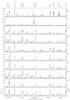 |
Fig. A.1 Spectra from the band 1 setup for all ten sources. The strongest lines are identified at the top of the figure. The red line indicates the zero level. This figure is identical to Fig. 2 and is reproduced here for completeness of the appendix. |
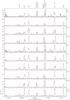 |
Fig. A.2 Spectra from the band 2 setup for all ten sources. |
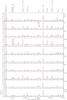 |
Fig. A.3 Spectra from the band 3 setup for all ten sources. |
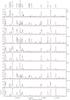 |
Fig. A.4 Spectra from the band 4 setup for all ten sources. |
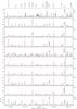 |
Fig. A.5 Spectra from the band 5 setup for all ten sources. A ~250 MHz overlap with Fig. A.6 is present, due to an incorrect setup. |
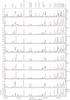 |
Fig. A.6 Spectra from the band 6 setup for all ten sources. |
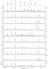 |
Fig. A.7 Spectra from the band 7 setup for all ten sources. |
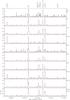 |
Fig. A.8 Spectra from the band 8 setup for all ten sources. |
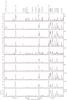 |
Fig. A.9 Spectra from the band 9 setup for all ten sources. |
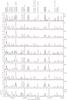 |
Fig. A.10 Spectra from the band 10 setup for all ten sources. |
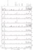 |
Fig. A.11 Spectra from the band 11 setup for all ten sources. |
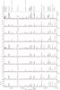 |
Fig. A.12 Spectra from the band 12 setup for all ten sources. |
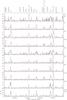 |
Fig. A.13 Spectra from the band 13 setup for all ten sources. |
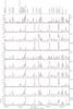 |
Fig. A.14 Spectra from the band 14 setup for all ten sources. |
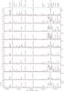 |
Fig. A.15 Spectra from the band 15 setup for all ten sources. |
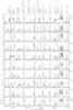 |
Fig. A.16 Spectra from the band 16 setup for all ten sources. |
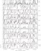 |
Fig. A.17 Spectra from the band 1 setup for all ten sources with a fixed maximum temperature scale of 5 K to highlight the weaker lines. The red line indicates the 0 K (continuum-removed) level.This figure is identical to Fig. 3 and is reproduced here for completeness of the appendix. |
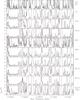 |
Fig. A.18 Spectra from the band 2 setup for all ten sources with a fixed maximum temperature scale of 5 K to highlight the weaker lines. The red line indicates the 0 K (continuum-removed) level. |
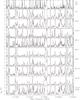 |
Fig. A.19 Spectra from the band 3 setup for all ten sources with a fixed maximum temperature scale of 5 K to highlight the weaker lines. The red line indicates the 0 K (continuum-removed) level. |
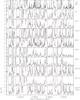 |
Fig. A.20 Spectra from the band 4 setup for all ten sources with a fixed maximum temperature scale of 5 K to highlight the weaker lines. The red line indicates the 0 K (continuum-removed) level. |
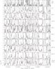 |
Fig. A.21 Spectra from the band 5 setup for all ten sources with a fixed maximum temperature scale of 5 K to highlight the weaker lines. A ~250 MHz overlap with Fig. A.22 is present, due to an incorrect setup. The red line indicates the 0 K (continuum-removed) level. |
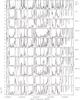 |
Fig. A.22 Spectra from the band 6 setup for all ten sources with a fixed maximum temperature scale of 5 K to highlight the weaker lines. The red line indicates the 0 K (continuum-removed) level. |
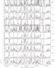 |
Fig. A.23 Spectra from the band 7 setup for all ten sources with a fixed maximum temperature scale of 5 K to highlight the weaker lines. The red line indicates the 0 K (continuum-removed) level. |
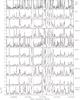 |
Fig. A.24 Spectra from the band 8 setup for all ten sources with a fixed maximum temperature scale of 5 K to highlight the weaker lines. The red line indicates the 0 K (continuum-removed) level. |
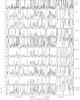 |
Fig. A.25 Spectra from the band 9 setup for all ten sources with a fixed maximum temperature scale of 5 K to highlight the weaker lines. The red line indicates the 0 K (continuum-removed) level. |
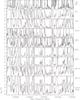 |
Fig. A.26 Spectra from the band 10 setup for all ten sources with a fixed maximum temperature scale of 5 K to highlight the weaker lines. The red line indicates the 0 K (continuum-removed) level. |
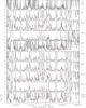 |
Fig. A.27 Spectra from the band 11 setup for all ten sources with a fixed maximum temperature scale of 5 K to highlight the weaker lines. The red line indicates the 0 K (continuum-removed) level. |
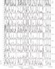 |
Fig. A.28 Spectra from the band 12 setup for all ten sources with a fixed maximum temperature scale of 5 K to highlight the weaker lines. The red line indicates the 0 K (continuum-removed) level. |
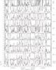 |
Fig. A.29 Spectra from the band 13 setup for all ten sources with a fixed maximum temperature scale of 5 K to highlight the weaker lines. The red line indicates the 0 K (continuum-removed) level. |
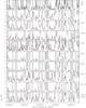 |
Fig. A.30 Spectra from the band 14 setup for all ten sources with a fixed maximum temperature scale of 5 K to highlight the weaker lines. The red line indicates the 0 K (continuum-removed) level. |
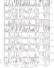 |
Fig. A.31 Spectra from the band 15 setup for all ten sources with a fixed maximum temperature scale of 5 K to highlight the weaker lines. The red line indicates the 0 K (continuum-removed) level. |
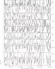 |
Fig. A.32 Spectra from the band 16 setup for all ten sources with a fixed maximum temperature scale of 5 K to highlight the weaker lines. The red line indicates the 0 K (continuum-removed) level. |
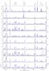 |
Fig. A.33 Spectra from the band 1 setup for all ten sources with the summation of fits to individual species in blue. The strongest lines are identified at the top of the figure. |
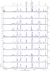 |
Fig. A.34 Spectra from the band 2 setup for all ten sources with the summation of fits to individual species in blue. |
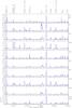 |
Fig. A.35 Spectra from the band 3 setup for all ten sources with the summation of fits to individual species in blue. |
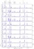 |
Fig. A.36 Spectra from the band 4 setup for all ten sources with the summation of fits to individual species in blue. |
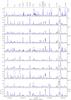 |
Fig. A.37 Spectra from the band 5 setup for all ten sources with the summation of fits to individual species in blue. A ~250 MHz overlap with Fig. A.38 is present, due to an incorrect setup. |
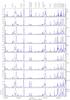 |
Fig. A.38 Spectra from the band 6 setup for all ten sources with the summation of fits to individual species in blue except for CH3CN which must be fitted with a non-LTE model and is therefore not added here (see Sect. 4.3). |
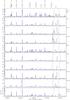 |
Fig. A.39 Spectra from the band 7 setup for all ten sources. |
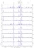 |
Fig. A.40 Spectra from the band 8 setup for all ten sources with the summation of fits to individual species in blue. |
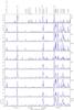 |
Fig. A.41 Spectra from the band 9 setup for all ten sources with the summation of fits to individual species in blue. |
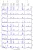 |
Fig. A.42 Spectra from the band 10 setup for all ten sources with the summation of fits to individual species in blue. |
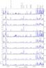 |
Fig. A.43 Spectra from the band 11 setup for all ten sources with the summation of fits to individual species in blue. |
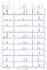 |
Fig. A.44 Spectra from the band 12 setup for all ten sources with the summation of fits to individual species in blue. |
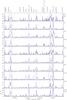 |
Fig. A.45 Spectra from the band 13 setup for all ten sources with the summation of fits to individual species in blue. |
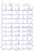 |
Fig. A.46 Spectra from the band 14 setup for all ten sources with the summation of fits to individual species in blue. |
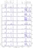 |
Fig. A.47 Spectra from the band 15 setup for all ten sources with the summation of fits to individual species in blue. |
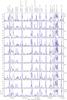 |
Fig. A.48 Spectra from the band 16 setup for all ten sources with the summation of fits to individual species in blue. |
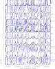 |
Fig. A.49 Spectra from the band 1 setup for all ten sources with the summation of fits to individual species in blue and with a fixed maximum temperature scale of 5 K to highlight the weaker lines. The red line indicates the 0 K (continuum-removed) level. |
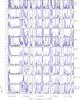 |
Fig. A.50 Spectra from the band 2 setup for all ten sources with the summation of fits to individual species in blue and with a fixed maximum temperature scale of 5 K to highlight the weaker lines. The red line indicates the 0 K (continuum-removed) level. |
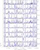 |
Fig. A.51 Spectra from the band 3 setup for all ten sources with the summation of fits to individual species in blue and with a fixed maximum temperature scale of 5 K to highlight the weaker lines. The red line indicates the 0 K (continuum-removed) level. |
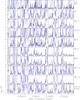 |
Fig. A.52 Spectra from the band 4 setup for all ten sources with the summation of fits to individual species in blue and with a fixed maximum temperature scale of 5 K to highlight the weaker lines. The red line indicates the 0 K (continuum-removed) level. |
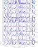 |
Fig. A.53 Spectra from the band 5 setup for all ten sources with the summation of fits to individual species in blue and with a fixed maximum temperature scale of 5 K to highlight the weaker lines. CH3CN is not included because it must be fitted with a non-LTE model and is therefore not added here (see Sect. 4.3). A ~250 MHz overlap with Fig. A.54 is present, due to an incorrect setup. The red line indicates the 0 K (continuum-removed) level. |
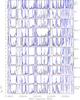 |
Fig. A.54 Spectra from the band 6 setup for all ten sources with the summation of fits to individual species in blue and with a fixed maximum temperature scale of 5 K to highlight the weaker lines. The red line indicates the 0 K (continuum-removed) level. |
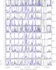 |
Fig. A.55 Spectra from the band 7 setup for all ten sources with the summation of fits to individual species in blue and with a fixed maximum temperature scale of 5 K to highlight the weaker lines. The red line indicates the 0 K (continuum-removed) level. |
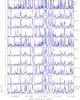 |
Fig. A.56 Spectra from the band 8 setup for all ten sources with the summation of fits to individual species in blue and with a fixed maximum temperature scale of 5 K to highlight the weaker lines. The red line indicates the 0 K (continuum-removed) level. |
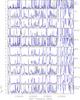 |
Fig. A.57 Spectra from the band 9 setup for all ten sources with the summation of fits to individual species in blue and with a fixed maximum temperature scale of 5 K to highlight the weaker lines. The red line indicates the 0 K (continuum-removed) level. |
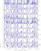 |
Fig. A.58 Spectra from the band 10 setup for all ten sources with the summation of fits to individual species in blue and with a fixed maximum temperature scale of 5 K to highlight the weaker lines. The red line indicates the 0 K (continuum-removed) level. |
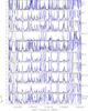 |
Fig. A.59 Spectra from the band 11 setup for all ten sources with a fixed maximum temperature scale of 5 K to highlight the weaker lines. The red line indicates the 0 K (continuum-removed) level. |
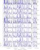 |
Fig. A.60 Spectra from the band 12 setup for all ten sources with the summation of fits to individual species in blue and with a fixed maximum temperature scale of 5 K to highlight the weaker lines. The red line indicates the 0 K (continuum-removed) level. |
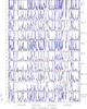 |
Fig. A.61 Spectra from the band 13 setup for all ten sources with the summation of fits to individual species in blue and with a fixed maximum temperature scale of 5 K to highlight the weaker lines. The red line indicates the 0 K (continuum-removed) level. |
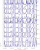 |
Fig. A.62 Spectra from the band 14 setup for all ten sources with the summation of fits to individual species in blue and with a fixed maximum temperature scale of 5 K to highlight the weaker lines. The red line indicates the 0 K (continuum-removed) level. |
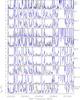 |
Fig. A.63 Spectra from the band 15 setup for all ten sources with the summation of fits to individual species in blue and with a fixed maximum temperature scale of 5 K to highlight the weaker lines. The red line indicates the 0 K (continuum-removed) level. |
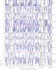 |
Fig. A.64 Spectra from the band 16 setup for all ten sources with the summation of fits to individual species in blue and with a fixed maximum temperature scale of 5 K to highlight the weaker lines. The red line indicates the 0 K (continuum-removed) level. |
Appendix B: List of species included in this study
Molecules studied in this paper, grouped by number of atoms.
All Tables
All Figures
|
Fig. 1 Continuum flux image of Orion-KL at ~1.3 mm, from an assemblage of channels free of line emission. The contours are every 100 mJy/beam (uncorrected for primary beam coupling). The ten sources analyzed in detail in this work are indicated and labeled (other labels of the same sources can be found in SIMBAD/CDS): HC = hot core, CR = compact ridge, MFxx from Favre et al. (2011a), Cxx from Friedel & Weaver (2011), IRcxx from Rieke et al. (1973), Shuping et al. (2004), mmxx from Feng et al. (2015) and references therein. The yellow cross indicates the center of explosion from which the BN, I, and n sources (marked by yellow stars) are moving away (Gómez et al. 2005). The blue circles mark the primary beam coupling efficiency (though the size changes by ±8% with frequency, decreasing with increasing frequency, we keep the same median case for all the figures). The primary beam coupling correction is not applied in the present and following figures. |
| In the text | |
|
Fig. 2 Spectra from the band 1 setup for all ten sources. The red line indicates the 0 K (continuum-removed) level. |
| In the text | |
|
Fig. 3 Spectra from the band 1 setup for all ten sources with a fixed maximum temperature scale of 5 K to highlight the weaker lines. The red line indicates the 0 K (continuum-removed) level. |
| In the text | |
|
Fig. 4 Detection of n-C3H7CN propyl cyanide isomer towards IRc21 (see map Fig. 1). In this and the following figures, the most intense lines are displayed (i.e. lines typically stronger than ~5σ. Weaker lines are hardly or not at all detectable and have no impact on the results, nor do lines blended with much stronger lines of other species). The data are in black and the fit is in red. The summation of the fit of all the species we have identified is displayed in blue. |
| In the text | |
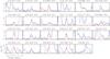 |
Fig. 5 Same as Fig. 4 for the detection of the i-C3H7CN propyl cyanide isomer. |
| In the text | |
|
Fig. 6 Integrated intensity map of the 236.990 GHz set of the n-C3H7CN isomer transitions (white contours) superimposed on the continuum map. The emission toward IRc7 and IRc21 and part of the emission toward MF2 are due to this species. Emission in other regions, especially the relatively strong emission seen toward CR/MF1 is due to emission from other molecular species at different velocities and appearing at the same frequency. |
| In the text | |
|
Fig. 7 CR/MF1 display of expected n-C3H7CN components. Despite the coincidental emission peak towards CR/MF1 in Fig. 6 that is visible in the 236.99 GHz window, n-C3H7CN is not detected in this source at a similar level to that seen in IRc21 (Fig. 4). Color-coding and TMB scale as in Fig. 4. |
| In the text | |
|
Fig. 8 Cyanoacetylene (HC3N) vibrationally excited transitions towards the HC. The fits help to trace the components, but have limited physical significance because their temperature is not constrained. The ν7 = 1 line at 218.861 or 237.093 GHz displays a shoulder due to the ν6 = 1 at 218.854 and 237.086 GHz, respectively). Color-coding as in Fig. 4. |
| In the text | |
|
Fig. 9 Integrated line intensity of cyanoacetylene vibrational modes (from ν= 0 to ν6 = ν7 = 1 (white contours) superimposed on the continuum image of the region). In the ν6 = ν7 = 1 image, contours towards CR/MF1, MF2, MF4, MF5, and MF12 are not related to HC3N. |
| In the text | |
|
Fig. 10 Singly 13C substituted cyanoacetylene isotopologue lines in fundamental and first vibrationally excited modes towards IRc21. The H13CCCN ν6 = 1 mode has no transition in our bands. Color-coding as in Fig. 4. |
| In the text | |
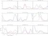 |
Fig. 11 Methylamine (CH3NH2) emission towards the hot core. Color-coding as in Fig. 4. |
| In the text | |
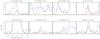 |
Fig. 12 Cyanamide (NH2CN) detection towards the EGP. Color-coding as in Fig. 4. |
| In the text | |
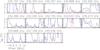 |
Fig. 13 Tentative detection of glycolaldehyde (CH2(OH)CHO) towards MF2. Color coding as in Fig. 4. |
| In the text | |
|
Fig. 14 Tentative detection of the 13C doubly substituted cyanoacetylene isotopologue lines towards IRc21. Color-coding as in Fig. 4. |
| In the text | |
|
Fig. 15 Possible H13CNH+ line towards CR/MF1. The line is present at both LSR velocities (axis above figure) for this source. |
| In the text | |
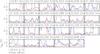 |
Fig. 16 Tentative detection of propanal towards IRc21. Color coding as in Fig. 4. |
| In the text | |
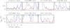 |
Fig. 17 Tentative detection of propenal towards IRc21. Color coding as in Fig. 4. |
| In the text | |
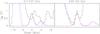 |
Fig. 18 Highly tentative detection of propynal towards the EGP. Color coding as in Fig. 4. |
| In the text | |
|
Fig. 19 Observations of hexatriynyl (C6H) towards SMA1 following the Feng et al. (2015) tentative detection. The three lines presented by Feng et al. (2015) are marked by thick boxes. Data are in black, the C6H model following the Feng et al. (2015) parameters in red, and its combination with vinyl cyanide at 230.108 GHz in cyan. |
| In the text | |
|
Fig. 20 Observations of hexatriynyl (C6H) towards the HC. The three lines presented by Feng et al. (2015) are marked by thick boxes. Data are in black, C6H modeling in red, and other species modeled in blue. The combination of C6H and vinyl cyanide emission at 230.109 GHz is shown in cyan. |
| In the text | |
|
Fig. 21 Observations towards the HC7N peak found by Feng et al. (2015) of the 12 cyanohexatryine (HC7N) transitions recorded in our survey. Three of the four lines presented by Feng et al. (2015) are marked by thick boxes (the last one is missing from our survey). Data are in black, HC7N model following the Feng et al. (2015) parameters in red. |
| In the text | |
|
Fig. 22 Observations towards the HC of the 12 cyanohexatryine (HC7N) transitions recorded in our survey. Three of the four lines within the Feng et al. (2015) survey are marked by thick boxes. Data are in black, HC7N model following the Feng et al. (2015) parameters in red, other species modeling in blue. |
| In the text | |
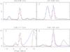 |
Fig. 23 Observations of formic acid (HCOOH) towards IRc21. Color-coding as in Fig. 4. |
| In the text | |
|
Fig. 24 Integrated intensity map of formic acid (HCOOH) emission at 220.038 GHz (white contours) superimposed on the continuum emission map. The main emission peaks are centered on IRc21 (compact emission) and on the EGP (Et. glycol) with an extension outside of the region. |
| In the text | |
|
Fig. 25 16O18O observations towards MF4. The expected line is traced in red together with the data (black) and LTE modeling of other species (blue). The parameters for these species have been adjusted from other components and do not exactly match the present lines because of the simplicity of the LTE model. |
| In the text | |
|
Fig. 26 Hydroxylamine (NH2OH) line observation 0.̋9 west of the EGP. The six red arrows mark the positions of the nine NH2OH lines (three lines are a combination of two transitions with very little or no spacing). The one possible detection is zoomed. Color-coding as in Fig. 4. |
| In the text | |
|
Fig. 27 Methanol (CH3OH), vinyl cyanide (C2H3CN), and ethyl cyanide (C2H5CN) line profiles for the ten sources (see Fig. 1). The black line traces the data and the red line the LTE fit. The vertical dashed lines represent the velocity components introduced in the fit to match the observations. |
| In the text | |
|
Fig. 28 Velocities of the main components towards the ten sources in our study superimposed on a copy of Fig. 1. The alternating white and black arrows and figures have no meaning and are only used to separate more clearly the list of velocities at each spot. |
| In the text | |
|
Fig. 29 Line shape difference between methanol (CH3OH) and methyl formate (CH3OCHO) towards MF4 for different transitions of methanol (in black; the upper state energy (K) and the torsional mode are indicated to the right) compared to the same methyl formate line (in red) for reference. The blue line marks the 9 km s-1 average velocity of the region. |
| In the text | |
|
Fig. 30 Fit of CH3CN K components of the J: 12→11 rotational transition towards MF5. Upper panel: fit of four K ladder components. Lower level: three velocity components ordered differently on the line of sight to fit the observed profile of the K = 3 transition (scaled to visually match the observations). |
| In the text | |
|
Fig. 31 Different components in the KL region following the discussion in Sects. 4.4 and 4.5. The front view shows the continuum contours from Fig. 1 employing simple elliptical shapes to indicate the different parts of the cloud. The red ellipse includes the HC ridge, encompassing IRc21, MF10, MF6, MF2, and the glycol peak. The explosion center is indicated by the set of orange arrows, and the velocity shifts of both the bulk of the gas and the line wings are shown in the corresponding color. The respective position of MF12 (dark blue), IRc7 (green) and the HC group along the Z-axis is not known and the arrangement shown is arbitrary. The only constraint is that MF4 (purple)/MF5 (orange) be behind the explosion center and the rest of the components be in front along the Z-axis. We have also not given any inclination or bent shape to the HC ridge along the Z-axis. The CR/MF1 (cyan) source is supposed to be at least 10 000 AU in front but could also be behind. MF4 and MF5 are split into three blobs with small velocity arrows of increasing length (and possibly approaching the observer for the first MF5 blob) to illustrate that the farther away from the explosion center, the higher is the source’s velocity (see Table 3). |
| In the text | |
|
Fig. 32 Three methyl formate (CH3OCHO) components observed towards CR/MF1. Data are in black; individual components: narrow are in red, wide are in green, sum of the components are in blue. |
| In the text | |
|
Fig. A.1 Spectra from the band 1 setup for all ten sources. The strongest lines are identified at the top of the figure. The red line indicates the zero level. This figure is identical to Fig. 2 and is reproduced here for completeness of the appendix. |
| In the text | |
|
Fig. A.2 Spectra from the band 2 setup for all ten sources. |
| In the text | |
|
Fig. A.3 Spectra from the band 3 setup for all ten sources. |
| In the text | |
|
Fig. A.4 Spectra from the band 4 setup for all ten sources. |
| In the text | |
|
Fig. A.5 Spectra from the band 5 setup for all ten sources. A ~250 MHz overlap with Fig. A.6 is present, due to an incorrect setup. |
| In the text | |
|
Fig. A.6 Spectra from the band 6 setup for all ten sources. |
| In the text | |
|
Fig. A.7 Spectra from the band 7 setup for all ten sources. |
| In the text | |
|
Fig. A.8 Spectra from the band 8 setup for all ten sources. |
| In the text | |
|
Fig. A.9 Spectra from the band 9 setup for all ten sources. |
| In the text | |
|
Fig. A.10 Spectra from the band 10 setup for all ten sources. |
| In the text | |
|
Fig. A.11 Spectra from the band 11 setup for all ten sources. |
| In the text | |
|
Fig. A.12 Spectra from the band 12 setup for all ten sources. |
| In the text | |
|
Fig. A.13 Spectra from the band 13 setup for all ten sources. |
| In the text | |
|
Fig. A.14 Spectra from the band 14 setup for all ten sources. |
| In the text | |
|
Fig. A.15 Spectra from the band 15 setup for all ten sources. |
| In the text | |
|
Fig. A.16 Spectra from the band 16 setup for all ten sources. |
| In the text | |
|
Fig. A.17 Spectra from the band 1 setup for all ten sources with a fixed maximum temperature scale of 5 K to highlight the weaker lines. The red line indicates the 0 K (continuum-removed) level.This figure is identical to Fig. 3 and is reproduced here for completeness of the appendix. |
| In the text | |
|
Fig. A.18 Spectra from the band 2 setup for all ten sources with a fixed maximum temperature scale of 5 K to highlight the weaker lines. The red line indicates the 0 K (continuum-removed) level. |
| In the text | |
|
Fig. A.19 Spectra from the band 3 setup for all ten sources with a fixed maximum temperature scale of 5 K to highlight the weaker lines. The red line indicates the 0 K (continuum-removed) level. |
| In the text | |
|
Fig. A.20 Spectra from the band 4 setup for all ten sources with a fixed maximum temperature scale of 5 K to highlight the weaker lines. The red line indicates the 0 K (continuum-removed) level. |
| In the text | |
|
Fig. A.21 Spectra from the band 5 setup for all ten sources with a fixed maximum temperature scale of 5 K to highlight the weaker lines. A ~250 MHz overlap with Fig. A.22 is present, due to an incorrect setup. The red line indicates the 0 K (continuum-removed) level. |
| In the text | |
|
Fig. A.22 Spectra from the band 6 setup for all ten sources with a fixed maximum temperature scale of 5 K to highlight the weaker lines. The red line indicates the 0 K (continuum-removed) level. |
| In the text | |
|
Fig. A.23 Spectra from the band 7 setup for all ten sources with a fixed maximum temperature scale of 5 K to highlight the weaker lines. The red line indicates the 0 K (continuum-removed) level. |
| In the text | |
|
Fig. A.24 Spectra from the band 8 setup for all ten sources with a fixed maximum temperature scale of 5 K to highlight the weaker lines. The red line indicates the 0 K (continuum-removed) level. |
| In the text | |
|
Fig. A.25 Spectra from the band 9 setup for all ten sources with a fixed maximum temperature scale of 5 K to highlight the weaker lines. The red line indicates the 0 K (continuum-removed) level. |
| In the text | |
|
Fig. A.26 Spectra from the band 10 setup for all ten sources with a fixed maximum temperature scale of 5 K to highlight the weaker lines. The red line indicates the 0 K (continuum-removed) level. |
| In the text | |
|
Fig. A.27 Spectra from the band 11 setup for all ten sources with a fixed maximum temperature scale of 5 K to highlight the weaker lines. The red line indicates the 0 K (continuum-removed) level. |
| In the text | |
|
Fig. A.28 Spectra from the band 12 setup for all ten sources with a fixed maximum temperature scale of 5 K to highlight the weaker lines. The red line indicates the 0 K (continuum-removed) level. |
| In the text | |
|
Fig. A.29 Spectra from the band 13 setup for all ten sources with a fixed maximum temperature scale of 5 K to highlight the weaker lines. The red line indicates the 0 K (continuum-removed) level. |
| In the text | |
|
Fig. A.30 Spectra from the band 14 setup for all ten sources with a fixed maximum temperature scale of 5 K to highlight the weaker lines. The red line indicates the 0 K (continuum-removed) level. |
| In the text | |
|
Fig. A.31 Spectra from the band 15 setup for all ten sources with a fixed maximum temperature scale of 5 K to highlight the weaker lines. The red line indicates the 0 K (continuum-removed) level. |
| In the text | |
|
Fig. A.32 Spectra from the band 16 setup for all ten sources with a fixed maximum temperature scale of 5 K to highlight the weaker lines. The red line indicates the 0 K (continuum-removed) level. |
| In the text | |
|
Fig. A.33 Spectra from the band 1 setup for all ten sources with the summation of fits to individual species in blue. The strongest lines are identified at the top of the figure. |
| In the text | |
|
Fig. A.34 Spectra from the band 2 setup for all ten sources with the summation of fits to individual species in blue. |
| In the text | |
|
Fig. A.35 Spectra from the band 3 setup for all ten sources with the summation of fits to individual species in blue. |
| In the text | |
|
Fig. A.36 Spectra from the band 4 setup for all ten sources with the summation of fits to individual species in blue. |
| In the text | |
|
Fig. A.37 Spectra from the band 5 setup for all ten sources with the summation of fits to individual species in blue. A ~250 MHz overlap with Fig. A.38 is present, due to an incorrect setup. |
| In the text | |
|
Fig. A.38 Spectra from the band 6 setup for all ten sources with the summation of fits to individual species in blue except for CH3CN which must be fitted with a non-LTE model and is therefore not added here (see Sect. 4.3). |
| In the text | |
|
Fig. A.39 Spectra from the band 7 setup for all ten sources. |
| In the text | |
|
Fig. A.40 Spectra from the band 8 setup for all ten sources with the summation of fits to individual species in blue. |
| In the text | |
|
Fig. A.41 Spectra from the band 9 setup for all ten sources with the summation of fits to individual species in blue. |
| In the text | |
|
Fig. A.42 Spectra from the band 10 setup for all ten sources with the summation of fits to individual species in blue. |
| In the text | |
|
Fig. A.43 Spectra from the band 11 setup for all ten sources with the summation of fits to individual species in blue. |
| In the text | |
|
Fig. A.44 Spectra from the band 12 setup for all ten sources with the summation of fits to individual species in blue. |
| In the text | |
|
Fig. A.45 Spectra from the band 13 setup for all ten sources with the summation of fits to individual species in blue. |
| In the text | |
|
Fig. A.46 Spectra from the band 14 setup for all ten sources with the summation of fits to individual species in blue. |
| In the text | |
|
Fig. A.47 Spectra from the band 15 setup for all ten sources with the summation of fits to individual species in blue. |
| In the text | |
|
Fig. A.48 Spectra from the band 16 setup for all ten sources with the summation of fits to individual species in blue. |
| In the text | |
|
Fig. A.49 Spectra from the band 1 setup for all ten sources with the summation of fits to individual species in blue and with a fixed maximum temperature scale of 5 K to highlight the weaker lines. The red line indicates the 0 K (continuum-removed) level. |
| In the text | |
|
Fig. A.50 Spectra from the band 2 setup for all ten sources with the summation of fits to individual species in blue and with a fixed maximum temperature scale of 5 K to highlight the weaker lines. The red line indicates the 0 K (continuum-removed) level. |
| In the text | |
|
Fig. A.51 Spectra from the band 3 setup for all ten sources with the summation of fits to individual species in blue and with a fixed maximum temperature scale of 5 K to highlight the weaker lines. The red line indicates the 0 K (continuum-removed) level. |
| In the text | |
|
Fig. A.52 Spectra from the band 4 setup for all ten sources with the summation of fits to individual species in blue and with a fixed maximum temperature scale of 5 K to highlight the weaker lines. The red line indicates the 0 K (continuum-removed) level. |
| In the text | |
|
Fig. A.53 Spectra from the band 5 setup for all ten sources with the summation of fits to individual species in blue and with a fixed maximum temperature scale of 5 K to highlight the weaker lines. CH3CN is not included because it must be fitted with a non-LTE model and is therefore not added here (see Sect. 4.3). A ~250 MHz overlap with Fig. A.54 is present, due to an incorrect setup. The red line indicates the 0 K (continuum-removed) level. |
| In the text | |
|
Fig. A.54 Spectra from the band 6 setup for all ten sources with the summation of fits to individual species in blue and with a fixed maximum temperature scale of 5 K to highlight the weaker lines. The red line indicates the 0 K (continuum-removed) level. |
| In the text | |
|
Fig. A.55 Spectra from the band 7 setup for all ten sources with the summation of fits to individual species in blue and with a fixed maximum temperature scale of 5 K to highlight the weaker lines. The red line indicates the 0 K (continuum-removed) level. |
| In the text | |
|
Fig. A.56 Spectra from the band 8 setup for all ten sources with the summation of fits to individual species in blue and with a fixed maximum temperature scale of 5 K to highlight the weaker lines. The red line indicates the 0 K (continuum-removed) level. |
| In the text | |
|
Fig. A.57 Spectra from the band 9 setup for all ten sources with the summation of fits to individual species in blue and with a fixed maximum temperature scale of 5 K to highlight the weaker lines. The red line indicates the 0 K (continuum-removed) level. |
| In the text | |
|
Fig. A.58 Spectra from the band 10 setup for all ten sources with the summation of fits to individual species in blue and with a fixed maximum temperature scale of 5 K to highlight the weaker lines. The red line indicates the 0 K (continuum-removed) level. |
| In the text | |
|
Fig. A.59 Spectra from the band 11 setup for all ten sources with a fixed maximum temperature scale of 5 K to highlight the weaker lines. The red line indicates the 0 K (continuum-removed) level. |
| In the text | |
|
Fig. A.60 Spectra from the band 12 setup for all ten sources with the summation of fits to individual species in blue and with a fixed maximum temperature scale of 5 K to highlight the weaker lines. The red line indicates the 0 K (continuum-removed) level. |
| In the text | |
|
Fig. A.61 Spectra from the band 13 setup for all ten sources with the summation of fits to individual species in blue and with a fixed maximum temperature scale of 5 K to highlight the weaker lines. The red line indicates the 0 K (continuum-removed) level. |
| In the text | |
|
Fig. A.62 Spectra from the band 14 setup for all ten sources with the summation of fits to individual species in blue and with a fixed maximum temperature scale of 5 K to highlight the weaker lines. The red line indicates the 0 K (continuum-removed) level. |
| In the text | |
|
Fig. A.63 Spectra from the band 15 setup for all ten sources with the summation of fits to individual species in blue and with a fixed maximum temperature scale of 5 K to highlight the weaker lines. The red line indicates the 0 K (continuum-removed) level. |
| In the text | |
|
Fig. A.64 Spectra from the band 16 setup for all ten sources with the summation of fits to individual species in blue and with a fixed maximum temperature scale of 5 K to highlight the weaker lines. The red line indicates the 0 K (continuum-removed) level. |
| In the text | |
Current usage metrics show cumulative count of Article Views (full-text article views including HTML views, PDF and ePub downloads, according to the available data) and Abstracts Views on Vision4Press platform.
Data correspond to usage on the plateform after 2015. The current usage metrics is available 48-96 hours after online publication and is updated daily on week days.
Initial download of the metrics may take a while.