| Issue |
A&A
Volume 594, October 2016
Planck 2015 results
|
|
|---|---|---|
| Article Number | A18 | |
| Number of page(s) | 21 | |
| Section | Cosmology (including clusters of galaxies) | |
| DOI | https://doi.org/10.1051/0004-6361/201525829 | |
| Published online | 20 September 2016 | |
Planck 2015 results
XVIII. Background geometry and topology of the Universe
1 APC, AstroParticule et Cosmologie, Université Paris Diderot, CNRS/IN2P3, CEA/lrfu, Observatoire de Paris, Sorbonne Paris Cité, 10 rue Alice Domon et Léonie Duquet, 75205 Paris Cedex 13, France
2 Aalto University Metsähovi Radio Observatory and Dept of Radio Science and Engineering, PO Box 13000 00076 Aalto, Finland
3 African Institute for Mathematical Sciences, 6−8 Melrose Road, Muizenberg, Cape Town, South Africa
4 Agenzia Spaziale Italiana Science Data Center, via del Politecnico snc, 00133 Roma, Italy
5 Aix Marseille Université, CNRS, LAM (Laboratoire d’Astrophysique de Marseille) UMR 7326, 13388 Marseille, France
6 Astrophysics Group, Cavendish Laboratory, University of Cambridge, J J Thomson Avenue, Cambridge CB3 0HE, UK
7 Astrophysics & Cosmology Research Unit, School of Mathematics, Statistics & Computer Science, University of KwaZulu-Natal, Westville Campus, Private Bag X54001, 4000 Durban, South Africa
8 CGEE, SCS Qd 9, Lote C, Torre C, 4° andar, Ed. Parque Cidade Corporate, CEP 70308-200, Brasília, DF, Brazil
9 CITA, University of Toronto, 60 St. George St., Toronto, ON M5S 3H8, Canada
10 CNRS, IRAP, 9 Av. colonel Roche, BP 44346, 31028 Toulouse Cedex 4, France
11 CRANN, Trinity College, 2 Dublin, Ireland
12 California Institute of Technology, Pasadena, California, USA
13 Centre for Theoretical Cosmology, DAMTP, University of Cambridge, Wilberforce Road, Cambridge CB3 0WA, UK
14 Centro de Estudios de Física delCosmos de Aragón (CEFCA), Plaza San Juan, 1, planta 2, 44001 Teruel, Spain
15 Computational Cosmology Center, Lawrence Berkeley National Laboratory, Berkeley, CA94720 California, USA
16 Consejo Superior de Investigaciones Científicas (CSIC), 28006 Madrid, Spain
17 DSM/Irfu/SPP, CEA-Saclay, 91191 Gif-sur-Yvette Cedex, France
18 DTU Space, National Space Institute, Technical University of Denmark, Elektrovej 327, 2800 Kgs. Lyngby, Denmark
19 Département de Physique Théorique, Université de Genève, 24 Quai E. Ansermet, 1211 Genève 4, Switzerland
20 Departamento de Astrofísica, Universidad de La Laguna (ULL), 38206 La Laguna, Tenerife, Spain
21 Departamento de Física, Universidad de Oviedo, Avda. Calvo Sotelo s/n, 33003 Oviedo, Spain
22 Department of Astronomy and Astrophysics, University of Toronto, 50 Saint George Street, Toronto, ONMSS Ontario, Canada
23 Department of Astrophysics/IMAPP, Radboud University Nijmegen, PO Box 9010, 6500 GL Nijmegen, The Netherlands
24 Department of Physics & Astronomy, University of British Columbia, 6224 Agricultural Road, Vancouver, British Columbia, Canada
25 Department of Physics and Astronomy, Dana and David Dornsife College of Letter, Arts and Sciences, University of Southern California, Los Angeles, CA 90089, USA
26 Department of Physics and Astronomy, University College London, London WC1E 6BT, UK
27 Department of Physics, Florida State University, Keen Physics Building, 77 Chieftan Way, Tallahassee, Florida, USA
28 Department of Physics, Gustaf Hällströmin katu 2a, University of Helsinki, 00100 Helsinki, Finland
29 Department of Physics, Princeton University, Princeton, New Jersey NJ 08544, USA
30 Department of Physics, University of Alberta, 11322-89 Avenue, Edmonton, Alberta, T6G 2G7, Canada
31 Department of Physics, University of California, Santa Barbara, California CA 93106, USA
32 Department of Physics, University of Illinois at Urbana-Champaign, 1110 West Green Street, Urbana, Illinois, USA
33 Dipartimento di Fisica e Astronomia G. Galilei, Università degli Studi di Padova, via Marzolo 8, 35131 Padova, Italy
34 Dipartimento di Fisica e Scienze della Terra, Università di Ferrara, via Saragat 1, 44122 Ferrara, Italy
35 Dipartimento di Fisica, Università La Sapienza, P.le A. Moro 2, Roma, Italy
36 Dipartimento di Fisica, Università degli Studi di Milano, via Celoria, 16 Milano, Italy
37 Dipartimento di Fisica, Università degli Studi di Trieste, via A. Valerio 2, Trieste, Italy
38 Dipartimento di Matematica, Università di Roma Tor Vergata, via della Ricerca Scientifica 1, Roma, Italy
39 Discovery Center, Niels Bohr Institute, Blegdamsvej 17, Copenhagen, Denmark
40 Discovery Center, Niels Bohr Institute, Copenhagen University, Blegdamsvej 17, Copenhagen, Denmark
41 European Space Agency, ESAC, Planck Science Office, Camino bajo del Castillo, s/n, Urbanización Villafranca del Castillo, Villanueva de la Cañada, 28692 Madrid, Spain
42 European Space Agency, ESTEC, Keplerlaan 1, 2201 AZ Noordwijk, The Netherlands
43 Gran Sasso Science Institute, INFN, viale F. Crispi 7, 67100 L’ Aquila, Italy
44 HGSFP and University of Heidelberg, Theoretical Physics Department, Philosophenweg 16, 69120 Heidelberg, Germany
45 Helsinki Institute of Physics, Gustaf Hällströmin katu 2, University of Helsinki, Helsinki, Finland
46 INAF−Osservatorio Astronomico di Padova, Vicolo dell’Osservatorio 5, Padova, Italy
47 INAF−Osservatorio Astronomico di Roma, via di Frascati 33, Monte Porzio Catone, Italy
48 INAF−Osservatorio Astronomico di Trieste, via G.B. Tiepolo 11, Trieste, Italy
49 INAF/IASF Bologna, via Gobetti 101, Bologna, Italy
50 INAF/IASF Milano, via E. Bassini 15, Milano, Italy
51 INFN, Sezione di Bologna, viale Berti Pichat 6/2, 40127 Bologna, Italy
52 INFN, Sezione di Ferrara, via Saragat 1, 44122 Ferrara, Italy
53 INFN, Sezione di Roma 1, Università di Roma Sapienza, Piazzale Aldo Moro 2, 00185, Roma, Italy
54 INFN, Sezione di Roma 2, Università di Roma Tor Vergata, via della Ricerca Scientifica 1, Roma, Italy
55 INFN/National Institute for Nuclear Physics, via Valerio 2, 34127 Trieste, Italy
56 IPAG: Institut de Planétologie et d’Astrophysique de Grenoble, Université Grenoble Alpes, IPAG; CNRS, IPAG, 38000 Grenoble, France
57 IUCAA, Post Bag 4, Ganeshkhind, Pune University Campus, 411 007 Pune, India
58 Imperial College London, Astrophysics group, Blackett Laboratory, Prince Consort Road, London, SW7 2AZ, UK
59 Infrared Processing and Analysis Center, California Institute of Technology, Pasadena, CA 91125, USA
60 Institut Néel, CNRS, Université Joseph Fourier Grenoble I, 25 rue des Martyrs, Grenoble, France
61 Institut Universitaire de France, 103 Bd Saint-Michel, 75005 Paris, France
62 Institut d’Astrophysique Spatiale, CNRS, Univ. Paris-Sud, Université Paris-Saclay, Bât. 121, 91405 Orsay Cedex, France
63 Institut d’Astrophysique de Paris, CNRS (UMR 7095), 98 bis Boulevard Arago, 75014 Paris, France
64 Institut für Theoretische Teilchenphysik und Kosmologie, RWTH Aachen University, 52056 Aachen, Germany
65 Institute for Space Sciences, Bucharest-Magurale, 077125 Bucharest, Romania
66 Institute of Astronomy, University of Cambridge, Madingley Road, Cambridge CB3 0HA, UK
67 Institute of Theoretical Astrophysics, University of Oslo, 1072 Blindern, Oslo, Norway
68 Instituto de Astrofísica de Canarias, C/Vía Láctea s/n, La Laguna, 38205 Tenerife, Spain
69 Instituto de Física de Cantabria (CSIC-Universidad de Cantabria), Avda. de los Castros s/n, 39005 Santander, Spain
70 Istituto Nazionale di Fisica Nucleare, Sezione di Padova, via Marzolo 8, 35131 Padova, Italy
71 Jet Propulsion Laboratory, California Institute of Technology, 4800 Oak Grove Drive, Pasadena, California, USA
72 Jodrell Bank Centre for Astrophysics, Alan Turing Building, School of Physics and Astronomy, The University of Manchester, Oxford Road, Manchester, M13 9PL, UK
73 Kavli Institute for Cosmological Physics, University of Chicago, Chicago, IL 60637, USA
74 Kavli Institute for Cosmology Cambridge, Madingley Road, Cambridge, CB3 0HA, UK
75 Kazan Federal University, 18 Kremlyovskaya St., 420008 Kazan, Russia
76 LAL, Université Paris-Sud, CNRS/IN2P3, Orsay, France
77 LERMA, CNRS, Observatoire de Paris, 61 Avenue de l’Observatoire, Paris, France
78 Laboratoire AIM, IRFU/Service d’Astrophysique− CEA/DSM − CNRS − Université Paris Diderot, Bât. 709, CEA-Saclay, 1191 Gif-sur-Yvette Cedex, France
79 Laboratoire Traitement et Communication de l’Information, CNRS (UMR 5141) and Télécom ParisTech, 46 rue Barrault, 75634 Paris Cedex 13, France
80 Laboratoire de Physique Subatomique et Cosmologie, Université Grenoble-Alpes, CNRS/IN2P3, 53 rue des Martyrs, 38026 Grenoble Cedex, France
81 Laboratoire de Physique Théorique, Université Paris-Sud 11 & CNRS, Bâtiment 210, 91405 Orsay, France
82 Lawrence Berkeley National Laboratory, Berkeley, CA 94720 California, USA
83 Lebedev Physical Institute of the Russian Academy of Sciences, Astro Space Centre, 84/32 Profsoyuznaya st., 117997 Moscow, Russia
84 Max-Planck-Institut für Astrophysik, Karl-Schwarzschild-Str. 1, 85741 Garching, Germany
85 McGill Physics, Ernest Rutherford Physics Building, McGill University, 3600 rue University, Montréal, QC, H3A 2T8, Canada
86 Mullard Space Science Laboratory, University College London, Surrey RH5 6NT, UK
87 National University of Ireland, Department of Experimental Physics, Maynooth, Co. Kildare, Ireland
88 Nicolaus Copernicus Astronomical Center, Bartycka 18, 00-716 Warsaw, Poland
89 Niels Bohr Institute, Blegdamsvej 17, Copenhagen, Denmark
90 Niels Bohr Institute, Copenhagen University, Blegdamsvej 17, Copenhagen, Denmark
91 Nordita (Nordic Institute for Theoretical Physics), Roslagstullsbacken 23, 106 91 Stockholm, Sweden
92 Optical Science Laboratory, University College London, Gower Street, WC 1E6 BT London, UK
93 SISSA, Astrophysics Sector, via Bonomea 265, 34136 Trieste, Italy
94 SMARTEST Research Centre, Università degli Studi e-Campus, via Isimbardi 10, 22060 Novedrate (CO), Italy
95 School of Physics and Astronomy, Cardiff University, Queens Buildings, The Parade, Cardiff, CF24 3AA, UK
96 School of Physics and Astronomy, University of Nottingham, Nottingham NG7 2RD, UK
97 Sorbonne Université-UPMC, UMR7095, Institut d’Astrophysique de Paris, 98 bis Boulevard Arago, 75014 Paris, France
98 Space Sciences Laboratory, University of California, Berkeley, CA 94720 California, USA
99 Special Astrophysical Observatory, Russian Academy of Sciences, Nizhnij Arkhyz, Zelenchukskiy region, 369167 Karachai-Cherkessian Republic, Russia
100 Stanford University, Dept of Physics, Varian Physics Bldg, 382 via Pueblo Mall, Stanford, California, USA
101 Sub-Department of Astrophysics, University of Oxford, Keble Road, Oxford OX1 3RH, UK
102 The Oskar Klein Centre for Cosmoparticle Physics, Department of Physics, Stockholm University, AlbaNova, 106 91 Stockholm, Sweden
103 Theory Division, PH-TH, CERN, 1211 Geneva 23, Switzerland
104 UPMC Univ. Paris 06, UMR7095, 98 bis Boulevard Arago, 75014 Paris, France
105 Université de Toulouse, UPS-OMP, IRAP, 31028 Toulouse Cedex 4, France
106 University of Granada, Departamento de Física Teórica y del Cosmos, Facultad de Ciencias, 18010 Granada, Spain
107 University of Granada, Instituto Carlos I de Física Teórica y Computacional, Granada, Spain
108 Warsaw University Observatory, Aleje Ujazdowskie 4, 00-478 Warszawa, Poland
⋆
Corresponding author: A. H. Jaffe, e-mail: This email address is being protected from spambots. You need JavaScript enabled to view it.
Received: 6 February 2015
Accepted: 10 April 2016
Abstract
Maps of cosmic microwave background (CMB) temperature and polarization from the 2015 release of Planck data provide the highestquality full-sky view of the surface of last scattering available to date. This enables us to detect possible departures from a globally isotropic cosmology. We present the first searches using CMB polarization for correlations induced by a possible non-trivial topology with a fundamental domain that intersects, or nearly intersects, the last-scattering surface (at comoving distance χrec), both via a direct scan for matched circular patterns at the intersections and by an optimal likelihood calculation for specific topologies. We specialize to flat spaces with cubic toroidal (T3) and slab (T1) topologies, finding that explicit searches for the latter are sensitive to other topologies with antipodal symmetry. These searches yield no detection of a compact topology with a scale below the diameter of the last-scattering surface. The limits on the radius ℛi of the largest sphere inscribed in the fundamental domain (at log-likelihood ratio Δlnℒ > −5 relative to a simply-connected flat Planck best-fit model) are: ℛi > 0.97 χrec for the T3 cubic torus; and ℛi > 0.56 χrec for the T1 slab. The limit for the T3 cubic torus from the matched-circles search is numerically equivalent, ℛi > 0.97 χrec at 99% confidence level from polarization data alone. We also perform a Bayesian search for an anisotropic global Bianchi VIIh geometry. In the non-physical setting, where the Bianchi cosmology is decoupled from the standard cosmology, Planck temperature data favour the inclusion of a Bianchi component with a Bayes factor of at least 2.3 units of log-evidence. However, the cosmological parameters that generate this pattern are in strong disagreement with those found from CMB anisotropy data alone. Fitting the induced polarization pattern for this model to the Planck data requires an amplitude of −0.10 ± 0.04 compared to the value of + 1 if the model were to be correct. In the physically motivated setting, where the Bianchi parameters are coupled and fitted simultaneously with the standard cosmological parameters, we find no evidence for a Bianchi VIIh cosmology and constrain the vorticity of such models to (ω/H)0 < 7.6 × 10⁻¹⁰ (95% CL).
Key words: cosmic background radiation / cosmology: observations / cosmological parameters / gravitation / methods: data analysis / methods: statistical
© ESO, 2016
1. Introduction
This paper, one of a series associated with the 2015 release of Planck1 data, will present limits on departures from the global isotropy of spacetime. We assess anisotropic but homogeneous Bianchi cosmological models and non-trivial global topologies in the light of the latest temperature and polarization data.
In Planck Collaboration XXVI (2014), the limits came from the 2013 Planck cosmological data release: cosmic microwave background (CMB) intensity data collected over approximately one year. This work uses the 2015 Planck data: CMB intensity from the whole mission along with a subset of polarization data. The greater volume of intensity data will allow more restrictive limits on the possibility of topological scales that are slightly larger than the volume enclosed by the last-scattering surface (roughly the Hubble volume), probing the excess anisotropic correlations that would be induced at large angular scales were such a model to obtain. For cubic torus topologies, we can therefore observe explicit repeated patterns (matched circles) when the comoving length of an edge is less than twice the distance to the recombination surface,  (using units with c = 1 here and throughout). Polarization, on the other hand, which is largely generated during recombination itself, can provide a more sensitive probe of topological domains smaller than the Hubble volume.
Whereas the analysis of temperature data in multiply connected universes has been treated in some depth in the literature (see Planck Collaboration XXVI 2014, and references therein), the discussion of polarization has been less complete. This paper therefore extends our previous likelihood analysis to polarized data, updates the direct search for matched circles (Cornish et al. 2004) as discussed in Bielewicz et al. (2012), and uses these to present the first limits on global topology from polarized CMB data.
The cosmological properties of Bianchi models (Collins & Hawking 1973; Barrow et al. 1985), were initially discussed in the context of CMB intensity (Barrow 1986; Jaffe et al. 2006c,a; Pontzen 2009). As discussed in Planck Collaboration XXVI (2014), it is by now well known that the observed large-scale intensity pattern mimics that of a particular Bianchi VIIh model, albeit one with cosmological parameters that are quite different from those needed to reproduce other CMB and cosmological data. More recently the induced polarization patterns have been calculated (Pontzen & Challinor 2007; Pontzen 2009; Pontzen & Challinor 2011). In this paper, we analyse the complete Planck intensity data, and compare the polarization pattern induced by that anisotropic model to Planck polarization data.
We note that the lack of a strong detection of cosmic B-mode polarization already provides some information about the Bianchi models: the induced geometrical focusing does not distinguish between E and B and thus should produce comparable amounts of each (e.g., Pontzen 2009). This does not apply to topological models: the linear evolution of primordial perturbations guarantees that a lack of primordial tensor perturbations results in a lack of B-mode polarization – the transfer function is not altered by topology.
In Sect. 2, we discuss previous limits on anisotropic models from Planck and other experiments. In Sect. 3 we discuss the CMB signals generated in such models, generalized to both temperature and polarization. In Sect. 4 we describe the Planck data and simulations we use in this study, the different methods we apply to those data, and the validation checks performed on those simulations. In Sect. 5 we discuss the results and conclude in Sect. 6 with the outlook for application of these techniques to future data and broader classes of models.
2. Previous results
The first searches for non-trivial topology on cosmic scales looked for repeated patterns or individual objects in the distribution of galaxies (Sokolov & Shvartsman 1974; Fang & Sato 1983; Fagundes & Wichoski 1987; Lehoucq et al. 1996; Roukema 1996; Weatherley et al. 2003; Fujii & Yoshii 2011). Searches for topology using the CMB began with COBE (Bennett et al. 1996) and found no indications of a non-trivial topology on the scale of the last-scattering surface (e.g., Starobinskij 1993; Sokolov 1993; Stevens et al. 1993; de Oliveira-Costa & Smoot 1995; Levin et al. 1998; Bond et al. 1998b, 2000; Rocha et al. 2004; but see also Roukema 2000b,a). With the higher resolution and sensitivity of WMAP, there were indications of low power on large scales which could have had a topological origin (Jarosik et al. 2011; Luminet et al. 2003; Caillerie et al. 2007; Aurich 1999; Aurich et al. 2004, 2005, 2006, 2008; Aurich & Lustig 2013; Lew & Roukema 2008; Roukema et al. 2008; Niarchou et al. 2004), but this possibility was not borne out by detailed real- and harmonic-space analyses in two dimensions (Cornish et al. 2004; Key et al. 2007; Bielewicz & Riazuelo 2009; Dineen et al. 2005; Kunz et al. 2006; Phillips & Kogut 2006; Niarchou & Jaffe 2007). Most studies, including this work, have emphasized searches for fundamental domains with antipodal correlations; see Vaudrevange et al. (2012) for results from a general search for the patterns induced by non-trivial topology on scales within the volume defined by the last-scattering surface, and, for example, Aurich & Lustig (2014) for a recent discussion of other possible topologies.
For a more complete overview of the field, we direct the reader to Planck Collaboration XXVI (2014). In that work, we applied various techniques to the Planck 2013 intensity data. For topology, we showed that a fundamental topological domain smaller than the Hubble volume is strongly disfavoured. This was done in two ways: first, a direct likelihood calculation of specific topological models; and second, a search for the expected repeated “circles in the sky” (Cornish et al. 2004), calibrated by simply-connected simulations. Both of these showed that the scale of any possible topology must exceed roughly the distance to the last-scattering surface, χrec. For the cubic torus, we found that the radius of the largest sphere inscribed in the topological fundamental domain must be ℛi> 0.92 χrec (at log-likelihood ratio Δlnℒ > −5 relative to a simply-connected flat Planck 2013 best-fit model). The matched-circle limit on topologies predicting back-to-back circles was ℛi> 0.94 χrec at the 99% confidence level.
Prior to the present work, there have been some extensions of the search for cosmic topology to polarization data. In particular, Bielewicz et al. (2012; see also Riazuelo et al. 2006) extended the direct search for matched circles to polarized data and found that the available WMAP data had insufficient sensitivity to provide useful constraints.
For Bianchi VIIh models, in Planck Collaboration XXVI (2014) a full Bayesian analysis of the Planck 2013 temperature data was performed, following the methods of McEwen et al. (2013). It was concluded that a physically-motivated model was not favoured by the data. If considered as a phenomenological template (for which the parameters common to the standard stochastic CMB and the deterministic Bianchi VIIh component are not linked), it was shown that an unphysical Bianchi VIIh model is favoured, with a log-Bayes factor between 1.5 ± 0.1 and 2.8 ± 0.1 – equivalent to an odds ratio of between approximately 1:4 and 1:16 – depending of the component separation technique adopted. Prior to the analysis of Planck Collaboration XXVI (2014), numerous analyses of Bianchi models using COBE (Bennett et al. 1996) and WMAP (Jarosik et al. 2011) data had been performed (Bunn et al. 1996; Kogut et al. 1997; Jaffe et al. 2005, 2006a,c,b; Cayón et al. 2006; Land & Magueijo 2006; McEwen et al. 2006; Bridges et al. 2007; Ghosh et al. 2007; Pontzen & Challinor 2007; Bridges et al. 2008; McEwen et al. 2013), and a similar Bianchi template was found in the WMAP data, first by Jaffe et al. (2005) and then subsequently by others (Bridges et al. 2007; Bridges et al. 2008; McEwen et al. 2013). Pontzen & Challinor (2007) discussed the CMB polarization signal from Bianchi models, and showed some incompatibility with WMAP data due to the large amplitude of both E- and B-mode components. For a more detailed review of the analysis of Bianchi models we refer the reader to Planck Collaboration XXVI (2014).
3. CMB signals in anisotropic and multiply-connected universes
3.1. Topology
There is a long history of studying the possible topological compactification of Friedmann-Lemaître-Robertson-Walker (FLRW) cosmologies; we refer readers to overviews such as Levin (2002), Lachieze-Rey & Luminet (1995), and Riazuelo et al. (2004a,b) for mathematical and physical detail. The effect of a non-trivial topology is equivalent to considering the full (simply-connected) three dimensional spatial slice of the manifold (the covering space) as being tiled by identical repetitions of a shape which is finite in one or more directions, the fundamental domain. In flat universes, to which we specialize here, there are a finite number of possibilities, each described by one or more continuous parameters describing the size in different directions.
In this paper, we pay special attention to topological models in which the fundamental domain is a right-rectangular prism (the three-torus, also referred to as “T3”), possibly with one or two infinite dimensions (the T2 “chimney” or “rod”, and T1 “slab” models). We limit these models in a number of ways. We explicitly compute the likelihood of the length of the fundamental domain for the cubic torus. Furthermore, we consider the slab model as a proxy for other models in which the matched circles (or excess correlations) are antipodally aligned, similar to the “lens” spaces available in manifolds with constant positive curvature. These models are thus sensitive to tori with varying side lengths, including those with non-right-angle corners. In these cases, the likelihood would have multiple peaks, one for each of the aligned pairs; their sizes correspond to those of the fundamental domains and their relative orientation to the angles. These non-rectangular prisms will be discussed in more detail in Jaffe & Starkman (in prep.).
3.1.1. Computing the covariance matrices
In Planck Collaboration XXVI (2014) we computed the temperature-temperature (TT) covariance matrices by summing up all modes kn that are present given the boundary conditions imposed by the non-trivial topology. For a cubic torus, we have a three-dimensional wave vector kn = (2π/L)n for a triplet of integers n, with unit vector  and the harmonic-space covariance matrix
  (1)where
  is the temperature radiation transfer function (see, e.g., Bond & Efstathiou 1987; and Seljak & Zaldarriaga 1996).
It is straightforward to extend this method to include polarization, since the cubic topology affects neither the local physics that governs the transfer functions, nor the photon propagation. The only effect is the discretization of the modes. We can therefore simply replace the radiation transfer function for the temperature fluctuations with the one for polarization, and obtain ![Mathematical equation: \begin{eqnarray} \label{topocorrX} C_{\ell \ell'}^{m m' \, (XX')} \!\propto\! \sum_{\bf n} \Delta_{\ell}^{(X)}(k_n, \Delta\eta) \Delta_{\ell'}^{(X')}(k_n, \Delta\eta) P(k_n) Y_{\ell m}({\vec{\hat{k\,}}}) Y_{\ell' m'}^* ({\vec{\hat{k\,}}}) ,\nonumber\\[-3mm] \end{eqnarray}](/articles/aa/full_html/2016/10/aa25829-15/aa25829-15-eq29.png) (2)where X,X′ = E,T. We are justified in ignoring the possibility of B-mode polarization as it is sourced only by primordial gravitational radiation even in the presence of non-trivial topology. In this way we obtain three sets of covariance matrices: TT, TE, and EE. In addition, since the publication of Planck Collaboration XXVI (2014) we have optimized the cubic torus calculation by taking into account more of the symmetries. The resulting speed-up of about an order of magnitude allowed us to reach a higher resolution of ℓmax = 64.
(2)where X,X′ = E,T. We are justified in ignoring the possibility of B-mode polarization as it is sourced only by primordial gravitational radiation even in the presence of non-trivial topology. In this way we obtain three sets of covariance matrices: TT, TE, and EE. In addition, since the publication of Planck Collaboration XXVI (2014) we have optimized the cubic torus calculation by taking into account more of the symmetries. The resulting speed-up of about an order of magnitude allowed us to reach a higher resolution of ℓmax = 64.
The fiducial cosmology assumed in the calculation of the covariance matrices is a flat ΛCDM FLRW Universe with Hubble constant H0 = 100h km s-1 Mpc-1, where: h = 0.6719; scalar spectral index ns = 0.9635; baryon density Ωbh2 = 0.0221; cold dark matter density Ωch2 = 0.1197; and neutrino density Ωνh2 = 0.0006.
3.1.2. Relative information in the matrices
To assess the information content of the covariance matrices, we consider the Kullback-Leibler (KL) divergence (see, e.g., Kunz et al. 2006, 2008; and Planck Collaboration XXVI 2014, for further applications of the KL divergence to topology). The KL divergence between two probability distributions p1(x) and p2(x) is given by 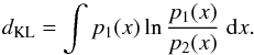 (3)If the two distributions are Gaussian with covariance matrices C1 and C2, this expression simplifies to
 ![Mathematical equation: \begin{equation} d_\mathrm{KL} = -\frac12 \left[\ln\left|\mtrx{C}_1 \mtrx{C}_2^{-1}\right| + \mathrm{Tr}\left(\mtrx{I} - \mtrx{C}_1 \mtrx{C}_2^{-1}\right)\right] , \end{equation}](/articles/aa/full_html/2016/10/aa25829-15/aa25829-15-eq46.png) (4)and is thus an asymmetric measure of the discrepancy between the covariance matrices. The KL divergence can be interpreted as the ensemble average of the log-likelihood ratio Δlnℒ between realizations of the two distributions. Hence, it enables us to probe the ability to tell if, on average, we can distinguish realizations of p1 from a fixed p2 without having to perform a brute-force Monte Carlo integration. Thus, the KL divergence is related to ensemble averages of the likelihood-ratio plots that we present for simulations (Sect. 4.4.1) and real data (Sect. 5.1) but can be calculated from the covariance matrices alone. Note that with this definition, the KL divergence is minimized for cases with the best match (maximal likelihood).
(4)and is thus an asymmetric measure of the discrepancy between the covariance matrices. The KL divergence can be interpreted as the ensemble average of the log-likelihood ratio Δlnℒ between realizations of the two distributions. Hence, it enables us to probe the ability to tell if, on average, we can distinguish realizations of p1 from a fixed p2 without having to perform a brute-force Monte Carlo integration. Thus, the KL divergence is related to ensemble averages of the likelihood-ratio plots that we present for simulations (Sect. 4.4.1) and real data (Sect. 5.1) but can be calculated from the covariance matrices alone. Note that with this definition, the KL divergence is minimized for cases with the best match (maximal likelihood).
In Planck Collaboration XXVI (2014) we used the KL divergence to show that the likelihood is robust to differences in the cosmological model and small differences in the topology.
In Fig. 1 we plot the KL divergence relative to an infinite Universe for the slab topology as a function of resolution ℓmax (upper panel) and fundamental domain size (lower panel). Our ability to detect a topology with a fundamental domain smaller than the distance to the last-scattering surface (approximately at the horizon distance  , so with sides of length
 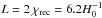 ) grows significantly with the resolution even beyond the cases that we studied. For the noise levels of the 2015 lowP data considered here and defined in Planck Collaboration XIII (2016), polarization maps do not add much information beyond that contained in the temperature maps, although, as also shown in Sect. 4.4.1, the higher sensitivity achievable by the full Planck low-ℓ data over all frequencies should enable even stronger constraints on these small fundamental domains.
If, however, the fundamental domain is larger than the horizon (as is the case for  ) then the relative information in the covariance matrix saturates quite early and a resolution of ℓmax ≃ 48 is actually sufficient. The main goal is thus to ensure that we have enough discriminatory power right up to the horizon size. In addition, polarization does not add much information in this case, irrespective of the noise level. This is to be expected: polarization is only generated for a short period of time around the surface of last scattering. Once the fundamental domain exceeds the horizon size, the relative information drops rapidly towards zero, and the dependence on ℓmax becomes weak.
In Fig. 2 we plot the KL divergence as a function of the size of the fundamental domain for fixed cube (T3), rod (T2), and slab (T1) topologies, each with fundamental domain size  , compared to the slab. Each shows a strong dip at , indicating the ability to detect this topology (although note the presence of a weaker dip around half the correct size,
  ). The figure also shows that ℓmax = 40 still shows the dip at the correct location, although somewhat more weakly than ℓmax = 80.
Note that the shape of the curves is essentially identical, with the slab likelihood able to detect one or more sets of antipodal matched circles (and their related excess correlations at large angular scales) present in each case. Figure 2 therefore shows that using the covariance matrix for a slab (T1) topology also allows detection of rod (T2) and cubic (T3) topologies: this is advantageous as the slab covariance matrix is considerably easier to calculate than the cube and rod, since it is only discretized in a single direction. Figure 3 shows the KL divergence as a function of the relative rotation of the fundamental domain, showing that, despite the lack of the full set of three pairs of antipodal correlations, we can determine the relative rotation of a single pair. This is exactly how the matched-circles tests work. Furthermore, as we will demonstrate in Sect. 4.4.1, slab likelihoods are indeed separately sensitive to the different sets of antipodal circles in cubic spaces. We can hence adopt the slab as the most general tool for searching for spaces with antipodal circles.
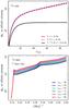 |
Fig. 1 KL divergence of slab (T1) topologies relative to an infinite Universe as a function of ℓmax with sizes |

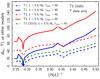 |
Fig. 2 KL divergence of fixed cubic, rod, and slab topologies with fundamental domain side |

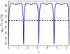 |
Fig. 3 KL divergence of a slab space relative to a cubic topology, as a function of rotation angle of the slab space (blue curve). Both spaces have |
3.2. Bianchi models
The polarization properties of Bianchi models were first derived in Pontzen & Challinor (2007) and extensively categorized in Pontzen (2009) and Pontzen & Challinor (2011). In these works it was shown that advection in Bianchi universes leads to efficient conversion of E-mode polarization to B modes; evidence for a significant Bianchi component found in temperature data would therefore suggest a large B-mode signal (but not necessarily require it; see Pontzen 2009). For examples of the temperature and polarization signatures of Bianchi VIIh models we refer the reader to Fig. 1 of Pontzen (2009). Despite the potential for CMB polarization to constrain the Bianchi sector, a full polarization analysis has not yet been carried out. The analysis of Pontzen & Challinor (2007) remains the state-of-the-art, where WMAP BB and EB power spectra were used to demonstrate (using a simple χ2 analysis) that a Bianchi VIIh model derived from temperature data was disfavoured compared to an isotropic model.
The subdominant, deterministic CMB contributions of Bianchi VIIh models can be characterized by seven parameters: the matter and dark energy densities, Ωm and ΩΛ, respectively; the present dimensionless vorticity, (ω/H)0; the dimensionless length-scale parameter, x, which controls the “tightness” of the characteristic Bianchi spirals; and the Euler angles2, (α,β,γ), describing their orientation (i.e., the choice of coordinate system), where H is the Hubble parameter. For further details see Planck Collaboration XXVI (2014), McEwen et al. (2013), Pontzen (2009), Pontzen & Challinor (2007), Jaffe et al. (2006c), Jaffe et al. (2005), and Barrow et al. (1985).
4. Methods
4.1. Data
In this work we use data from the Planck 2015 release. This includes intensity maps from the full mission, along with a subset of polarization data. Specifically, for the likelihood calculations discussed below (Sect. 4.3.1 for application to topology and Sect. 4.3.3 for Bianchi models) which rely on HEALPix maps at Nside = 16, we use the data designated “lowT,P”, as defined for the low-ℓPlanck likelihood for isotropic models (Planck Collaboration XI 2016; Planck Collaboration XIII 2016): lowP polarization maps based on the LFI 70 GHz channel and lowT temperature maps created by the Commander component separation method, along with the appropriate mask and noise covariance matrix. As in Planck Collaboration XXVI (2014), the intensity noise contribution is negligible on these scales, and diagonal regularizing noise with variance  has therefore been added to the intensity portion of the noise covariance matrix. We cut contaminated regions of the sky using the low-ℓ mask defined for the Planck isotropic likelihood code (Planck Collaboration XI 2016), retaining 94% of the sky for temperature, and the lowT,P polarization mask, cleaned with the templates created from Planck 30 GHz and 353 GHz data, retaining 47% of the sky for polarization.
The matched-circle search (Sects. 4.2 and 5.1.1) uses four component-separated maps (Planck Collaboration IX 2016) which effectively combine both intensity and polarization information from different scales. The maps are smoothed with a Gaussian filter of 30′ and 50′ full width at half maximum (FWHM) for temperature and polarization, respectively, and degraded to Nside = 512. Corresponding temperature and polarization common masks for diffuse emission, with a point source cut for the brightest sources, downgraded analogously to the maps, are used. After degradation, and accounting for the needed expansion of the polarization mask due to the conversion of Q and U to E, the temperature map retains 74% of the sky and the polarization map 40%. These E-mode maps are calculated using the method of Bielewicz et al. (2012; see also Kim 2011) and correspond to the spherical Laplacian of the scalar E, consequently filtering out power at large angular scales.
4.2. Topology: matched circles
As in Planck Collaboration XXVI (2014), we use the circle comparison statistic of Cornish et al. (1998), optimized for small-scale anisotropies (Cornish et al. 2004), to search for correlated circles in sky maps of the CMB temperature and polarization anisotropy. The circle comparison statistic uses the fact that the intersection of the topological fundamental domain with the surface of last scattering is a circle, potentially viewed from different directions in a multiply-connected Universe. Contrary to the temperature anisotropy, sourced by multiple terms at the last-scattering surface (i.e., the internal photon density fluctuations combined with the ordinary Sachs-Wolfe and Doppler effects), the CMB polarization anisotropy is sourced only by the quadrupole distribution of radiation scattering from free electrons at the moment of recombination (e.g., Kosowsky 1996). In particular, the recombination signal from polarization is only generated for a short time while there are enough electrons to scatter the photons but few enough for the plasma to be sufficiently transparent. Thus, in a multi-connected Universe the polarization signal does not exhibit the same cancellation of contributions from different terms as in the temperature anisotropy (Bielewicz et al. 2012). Polarization thus can provide a better opportunity for the detection of topological signatures than a temperature anisotropy map. There is a small subtlety here: whereas the intensity is a scalar and thus is unchanged when viewed from different directions, the polarization is a tensor which behaves differently under rotation. The polarization pattern itself depends on the viewing angle; hence, we need to use the coordinate-independent quantities, E and B, which are scalars (or pseudo-scalars) and are thus unchanged when viewed from different directions.
The decomposition into E and B of an arbitrary masked CMB polarization map, contaminated by noise, foregrounds, and systematic errors, is itself a computationally demanding task, non-local on the sky. Assuming negligible initial B polarization, we use only the E maps produced from component-separated CMB polarization maps using the same approach as Bielewicz et al. (2012).
Compared with the likelihood method described below, the circles search uses higher-resolution maps, and thus is sensitive out to a much higher maximum multipole, ℓmax. It is also potentially less sensitive to large-scale systematic errors, as the lowest multipoles are effectively filtered out: the polarization signal is weighted by a factor proportional to ℓ2 in the transformation from the Stokes parameters Q and U to an E-mode map. From the results of Sect. 3.1.2, this indicates that it uses more of the information available when confronting models with fundamental domains within the last-scattering surface compared to our implementation of the likelihood, limited to ℓmax ≃ 40. As we show in Sect. 4.4.1, this also allows the use of high-pass filtered component-separated maps (as defined in Planck Collaboration IX 2016) without a significant decrease in the ability to detect a multiply-connected topology.
The matched-circle statistic is defined by  (5)where Xi,m and Xj,m denote the Fourier coefficients of the temperature or E-mode fluctuations around two circles of angular radius α centred at different points on the sky, i and j, respectively, with relative phase φ∗. The mth harmonic of the field anisotropies around the circle is weighted by the factor | m |, taking into account the number of degrees of freedom per mode. Such weighting enhances the contribution of small-scale structure relative to large-scale fluctuations.
The S+ statistic corresponds to pairs of circles with the points ordered in a clockwise direction (phased). For the alternative ordering, when the points are ordered in an anti-clockwise direction (anti-phased along one of the circles), the Fourier coefficients Xi,m are complex conjugated, defining the S− statistic. This allows the detection of both orientable and non-orientable topologies. For orientable topologies the matched circles have anti-phased correlations, while for non-orientable topologies they have a mixture of anti-phased and phased correlations.
The S± statistics take values over the interval [− 1,1]. Circles that are perfectly matched have S = 1, while uncorrelated circles will have a mean value of S = 0. To find matched circles for each radius α, the maximum value  is determined.
Because general searches for matched circles are computationally very intensive, we restrict our analysis to a search for pairs of circles centred around antipodal points, so called back-to-back circles. The maps are also downgraded as described in Sect. 4.1. This increases the signal-to-noise ratio and greatly speeds up the computations required, but with no significant loss of discriminatory power. Regions most contaminated by Galactic foreground were removed from the analysis using the common temperature or polarization mask. More details on the numerical implementation of the algorithm can be found in Bielewicz & Banday (2011) and Bielewicz et al. (2012).
To draw any conclusions from an analysis based on the statistic  , it is very important to correctly estimate the threshold for a statistically significant match of circle pairs. We used 300 Monte Carlo simulations of the PlanckSMICA maps processed in the same way as the data to establish the threshold such that fewer than 1% of simulations would yield a false event. Note that we perform the entire analysis, including the final statistical calibration, separately for temperature and polarization.
4.3. Likelihood
4.3.1. Topology
For the likelihood analysis of the large-angle intensity and polarization data we have generalized the method implemented in Planck Collaboration XXVI (2014) to include polarization. The likelihood, i.e., the probability to find a combined temperature and polarization data map d with associated noise matrix N given a certain topological model T is then given by ![Mathematical equation: \begin{eqnarray} \label{eq:fullskylike} \lefteqn{P(\vec{d}| \mtrx{C}[\Theta_\mathrm{C},\Theta_\mathrm{T},T],A,\varphi)}\nonumber \\ && \propto \frac{1}{\sqrt{|A \mtrx{C} + \mtrx{ N}|}} \exp\left[- \frac{1}{2} \vec{d}^* (A \mtrx{ C} + \mtrx{ N} )^{-1} \vec{d} \right] , \end{eqnarray}](/articles/aa/full_html/2016/10/aa25829-15/aa25829-15-eq104.png) (6)where now d is a 3Npix-component data vector obtained by concatenation of the (I,Q,U) data sets while C and N are 3Npix × 3Npix theoretical signal and noise covariance matrices, arranged in block form as
(6)where now d is a 3Npix-component data vector obtained by concatenation of the (I,Q,U) data sets while C and N are 3Npix × 3Npix theoretical signal and noise covariance matrices, arranged in block form as  (7)Finally, ΘC is the set of standard cosmological parameters, ΘT is the set of topological parameters (e.g., the size, L, of the fundamental domain), ϕ is the orientation of the topology (e.g., the Euler angles), and A is a single amplitude, scaling the signal covariance matrix (this is equivalent to an overall amplitude in front of the power spectrum in the isotropic case). Working in pixel space allows for the straightforward application of an arbitrary mask, including separate masks for intensity and polarization parts of the data. The masking procedure can also be used to limit the analysis to intensity or polarization only.
Since C + N in pixel space is generally poorly conditioned, we again (following the 2013 procedure) project the data vector and covariance matrices onto a limited set of orthonormal basis vectors, select Nm such modes for comparison, and consider the likelihood marginalized over the remainder of the modes, ![Mathematical equation: \begin{eqnarray} \lefteqn{p( \fitdata | \mtrx{C}[\Theta_\mathrm{C},\Theta_\mathrm{T},T],\varphi, A) \propto} \nonumber \\ &&\frac{1}{\sqrt{|A \mtrx{ C} + \mtrx{ N} |_M}} \exp\left[- \frac{1}{2} \sum_{n=1}^{N_\mathrm{m}} d_n^* (A \mtrx{ C} + \mtrx{ N})^{-1}_{nn^\prime} d_{n^\prime} \right] \, , \label{eq:L_modes} \end{eqnarray}](/articles/aa/full_html/2016/10/aa25829-15/aa25829-15-eq118.png) (8)where C and N are restricted to the Nm × Nm subspace.
(8)where C and N are restricted to the Nm × Nm subspace.
The choice of the basis modes and their number Nm used for analysis is a compromise between robust invertibility of C + N and the amount of information retained. All the models for which likelihoods are compared must be expanded in the same set of modes. Thus, in Planck Collaboration XXVI (2014) we used the set of eigenmodes of the cut-sky covariance matrix of the fiducial best-fit simply-connected Universe, Cfid, as the analysis basis, limiting ourselves to the Nm modes with the largest eigenvalues. For comparison with the numbers we use, a full-sky temperature map with maximum multipole ℓmax has (ℓmax + 1)2−4 independent modes (four are removed to account for the unobserved monopole and dipole).
The addition of polarization data, with much lower signal-to-noise than the temperature, raises a new question: how is the temperature and polarization data mix reflected in the limited basis set we project onto? The most natural choice is the set of eigenmodes of the signal-to-noise matrix CfidN-1 for the fiducial model, and a restriction of the mode set based on signal-to-noise eigenvalues (see, e.g., Bond et al. 1998a). This, however, requires robust invertibility of the noise covariance matrix, which, again, is generally not the case for the smoothed data. Moreover, such a ranking by S/N would inevitably favour the temperature data, and we wish to explore the effect of including polarization data on an equal footing with temperature. We therefore continue to use the eigenmodes of the cut-sky fiducial covariance matrix as our basis. By default, we select the first Nm = 1085 eigenmodes (corresponding to ℓmax = 32), though we vary the mode count where it is informative to do so.
In Fig. 4 we show I, Q, and U maps of the highest-eigenvalue (i.e., highest contribution to the signal covariance) mode for our fiducial simply-connected model. Note that the scale is different for temperature compared to the two polarization maps: the temperature contribution to the mode is much greater than that of either polarization component. We show modes for the masked sky, although in fact the structure at large scales is similar to the full-sky case, rotated and adjusted somewhat to account for the mask. In Fig. 5 we show the structure of mode 301, with much lower signal amplitude (this particular mode was selected at random to indicate the relative ratios of temperature, polarization, and noise). Temperature remains dominant, although polarization begins to have a greater effect. Note that at this level of signal amplitude, the pattern is aligned with the mask, and shows a strong correlation between temperature and polarization.
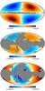 |
Fig. 4 Mode structure plotted as maps for the eigenvector corresponding to the highest-signal eigenvalue of the fiducial simply-connected model. The top map corresponds to temperature, middle to Q polarization, and bottom to U polarization. Masked pixels are plotted in grey. |
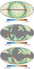 |
Fig. 5 Mode structure plotted as maps for the eigenvector corresponding to the 301st-highest-signal eigenvalue of the fiducial simply-connected model. The top map corresponds to temperature, middle to Q polarization, and bottom to U polarization. Masked pixels are plotted in grey. |
4.3.2. Evaluating the topological likelihood
The aim of the topological likelihood analysis is to calculate the likelihood as a function of the parameters pertaining to a particular topology, p(d | ΘT,T). To do so, we must marginalize over the other parameters appearing in Eq. (8), namely ΘC, ϕ, and A, as ![Mathematical equation: \begin{eqnarray} \lefteqn{p(\fitdata | \Theta_\mathrm{T}, T) =} \nonumber \\ && \int {\rm d} \Theta_\mathrm{C} \, {\rm d} \varphi \, {\rm d}A \, p( \fitdata | \mtrx{C}[\Theta_\mathrm{C}, \Theta_\mathrm{T},T],\varphi, A) \, p(\Theta_\mathrm{C},\varphi, A). \label{eq:L_marg_full} \end{eqnarray}](/articles/aa/full_html/2016/10/aa25829-15/aa25829-15-eq128.png) (9)The complexity of the topological covariance matrix calculation precludes a joint examination of the full cosmological and topological parameter spaces. Instead, we adopt the delta-function prior
(9)The complexity of the topological covariance matrix calculation precludes a joint examination of the full cosmological and topological parameter spaces. Instead, we adopt the delta-function prior  to fix the cosmological parameters at their fiducial values,
  (as defined in Sect. 3.1.1), and evaluate the likelihood on a grid of topological parameters using a restricted set of pre-calculated covariance matrices. We note that, as discussed in Planck Collaboration XXVI (2014), the ability to detect or rule out a multiply connected topology is insensitive to the values of the cosmological parameters adopted for the calculation of the covariance matrices.
In the setting described above, Eq. (9) simplifies to ![Mathematical equation: \begin{equation} p(\fitdata | \Theta_{\mathrm{T}, i}, T) = \int {\rm d} \varphi \, {\rm d}A \, p( \fitdata | \mtrx{C}[\Theta_\mathrm{C}^\star,\Theta_{\mathrm{T}, i},T],\varphi, A) \, p(\varphi, A), \label{eq:L_marg} \end{equation}](/articles/aa/full_html/2016/10/aa25829-15/aa25829-15-eq131.png) (10)where the likelihood at each gridpoint in topological parameter space, ΘT,i, is equal to the probability of obtaining the data given fixed cosmological and topological parameters and a compactification (i.e., fundamental domain shape and size), marginalized over orientation and amplitude. The calculation therefore reduces to evaluating the Bayesian evidence for a set of gridded topologies. As we focus on cubic torus and slab topologies in this work, we note that the sole topological parameter of interest is the size of the fundamental domain, L.
(10)where the likelihood at each gridpoint in topological parameter space, ΘT,i, is equal to the probability of obtaining the data given fixed cosmological and topological parameters and a compactification (i.e., fundamental domain shape and size), marginalized over orientation and amplitude. The calculation therefore reduces to evaluating the Bayesian evidence for a set of gridded topologies. As we focus on cubic torus and slab topologies in this work, we note that the sole topological parameter of interest is the size of the fundamental domain, L.
Even after fixing the cosmological parameters, calculating the Bayesian evidence is a time-consuming process, and is further complicated by the multimodal likelihood functions typical in non-trivial topologies. We therefore approach the problem on two fronts. We first approximate the likelihood function using a “profile likelihood” approach, as presented in Planck Collaboration XXVI (2014), in which the marginalization in Eq. (10) is replaced with maximization in the four-dimensional space of orientation and amplitude parameters. Specifically, we maximize the likelihood over the three angles defining the orientation of the fundamental domain using a three-dimensional Amoeba search (e.g., Press et al. 1992), where at each orientation the likelihood is separately maximized over the amplitude. Due to the complex structure of the likelihood surface in orientation space, we repeat this procedure five times with different starting orientations. This number of repetitions was chosen as a compromise between computational efficiency and assurance of statistical robustness, after testing of various strategies for the number of repetitions and the distribution of starting points, along with explicit extra runs to test outliers. To ensure uniform and non-degenerate coverage, the orientation space is traversed in a Cartesian projection of the northern hemisphere of the three-sphere S3 representation of rotations.
The profile likelihood calculation allows rapid evaluation of the likelihood and testing of different models compared with a variety of data and simulations, but it is difficult to interpret in a Bayesian setting. As we show below, however, the numerical results of profiling over this limited set of parameters agree numerically very well with the statistically correct marginalization procedure.
Our second approach explicitly calculates the marginalized likelihood, Eq. (10), allowing full Bayesian inference at the cost of increased computation time. We use the public MultiNest3 code (Feroz & Hobson 2008; Feroz et al. 2009, 2013) − optimized for exploring multimodal probability distributions in tens of dimensions − to compute the desired evidence values via nested sampling (Skilling 2004). MultiNest is run in its importance nested sampling mode (Feroz et al. 2013) using 200 live points, with tolerance and efficiency set to their recommended values of 0.5 and 0.3, respectively. The final ingredient needed to calculate the evidence values are priors for the marginalized parameters. We use a log prior for the amplitude, truncated to the range 0.1 ≤ A ≤ 10, and the Euler angles are defined to be uniform in 0 ≤ α< 2π, −1 ≤ cosβ ≤ 1, and 0 ≤ γ< 2π, respectively; MultiNest is able to wrap the priors on α and γ. The combined code will be made public as part of the AniCosmo4 package (McEwen et al. 2013).
It is worth noting that this formalism can be extended to compare models with different compactifications (or the simply connected model) using Bayesian model selection: the only additional requirements are priors for the topological parameters. Taking the current slab and cubic torus topologies as examples, by defining a prior on the size of the fundamental domain one can calculate the evidence for each model. Assuming each topology is equally likely a priori, i.e., that p(Tslab) = p(Tcub), one can then write down the relative probability of the two topologies given the data: 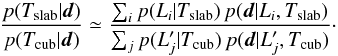 (11)Unfortunately, it is difficult to provide a physically-motivated proper prior distribution for the size of the fundamental domain. Even pleading ignorance and choosing a “naïve” uniform prior would require an arbitrary upper limit to L whose exact value would strongly influence the final conclusion. For this reason, we refrain from extending the formalism to model selection within this manuscript.
4.3.3. Bianchi models
While physically the cosmological densities describing Bianchi models should be identified with their standard ΛCDM counterparts, in previous analyses unphysical models have been considered in which the densities are allowed to differ. The first coherent analysis of Bianchi VIIh models was performed by McEwen et al. (2013), where the ΛCDM and Bianchi densities are coupled and all cosmological and Bianchi parameters are fit simultaneously. In the analysis of Planck Collaboration XXVI (2014), in order to compare with all prior studies both coupled and decoupled models were analysed. We consider the same two models here: namely, the physical open-coupled-Bianchi model where an open cosmology is considered (for consistency with the open Bianchi VIIh models), in which the Bianchi densities are coupled to their standard cosmological counterparts; and the phenomenological flat-decoupled-Bianchi model where a flat cosmology is considered and in which the Bianchi densities are decoupled.
We firstly carry out a full Bayesian analysis for these two Bianchi VIIh models, repeating the analysis performed in Planck Collaboration XXVI (2014) with updated Planck temperature data. The methodology is described in detail in McEwen et al. (2013) and summarized in Planck Collaboration XXVI (2014). The complete posterior distribution of all Bianchi and cosmological parameters is sampled and Bayesian evidence values are computed to compare Bianchi VIIh models to their concordance counterparts. Bianchi temperature signatures are simulated using the Bianchi25 code (McEwen et al. 2013), while the AniCosmo code is used to perform the analysis, which in turn uses MultiNest to sample the posterior distribution and compute evidence values.
To connect with polarization data, we secondly analyse polarization templates computed using the best-fit parameters from the analysis of temperature data. For the resulting small set of best-fit models, polarization templates are computed using the approach of Pontzen & Challinor (2007) and Pontzen (2009), and have been provided by Pontzen (priv. comm.). These Bianchi VIIh simulations are more accurate than those considered for the temperature analyses performed here and in previous works (see, e.g., Planck Collaboration XXVI 2014; McEwen et al. 2013; Bridges et al. 2008; Bridges et al. 2007; Jaffe et al. 2005, 2006a,b,c), since the recombination history is modelled. The overall morphology of the patterns are consistent between the codes; the strongest effect of incorporating the recombination history is its impact on the polarization fraction, although the amplitude of the temperature component can also vary by approximately 5% (which is calibrated in the current analysis, as described below).
Using the simulated Bianchi VIIh polarization templates computed following Pontzen & Challinor (2007) and Pontzen (2009), and provided by Pontzen (priv. comm.), we perform a maximum-likelihood fit for the amplitude of these templates using Planck polarization data (a full Bayesian evidence calculation of the complete temperature and polarization data set incorporating the more accurate Bianchi models of Pontzen & Challinor 2007; and Pontzen 2009, is left to future work). The likelihood in the Bianchi scenario is identical to that considered in Planck Collaboration XXVI (2014) and McEwen et al. (2013); however, we now consider the Bianchi and cosmological parameters fixed and simply introduce a scaling of the Bianchi template. The resulting likelihood reads: ![Mathematical equation: \begin{equation} P( \vec{d} \ \vert \ \lambda, \vec{t}) \propto \exp \biggl[-\frac{1}{2} (\vec{d} - \lambda \vec{t})^{\dagger} (\mtrx{C}+\mtrx{N})^{-1} (\vec{d} - \lambda \vec{t}) \biggr] , \end{equation}](/articles/aa/full_html/2016/10/aa25829-15/aa25829-15-eq141.png) (12)where d denotes the data vector,
(12)where d denotes the data vector,  is the Bianchi template for best-fit Bianchi parameters
  , C = C(ΘC) is the cosmological covariance matrix for the best-fit cosmological parameters
  , N is the noise covariance, and λ is the introduced scaling parameter (the effective vorticity of the scaled Bianchi component is simply λ(ω/H)0).
In order to effectively handle noise and partial sky coverage the data are analysed in pixel space. We restrict to polarization data only here since temperature data are used to determine the best-fit Bianchi parameters. The data and template vectors thus contain unmasked Q and U Stokes components only and, correspondingly, the cosmological and noise covariance matrices are given by the polarization (Q and U) subspace of Eq. (7), and again contain unmasked pixels only.
The maximum-likelihood (ML) estimate of the template amplitude is given by ![Mathematical equation: \hbox{$\lambda^{\rm ML} = \vec{t}^{\dagger} (\mtrx{C}+\mtrx{N})^{-1} \vec{d} / \left[\vec{t}^{\dagger}(\mtrx{C}+\mtrx{N})^{-1} \vec{t}\right]$}](/articles/aa/full_html/2016/10/aa25829-15/aa25829-15-eq148.png) and its dispersion by ΔλML = [t†(C + N)-1t] − 1 / 2 (see, e.g., Kogut et al. 1997; Jaffe et al. 2005). If Planck polarization data support the best-fit Bianchi model found from the analysis of temperature data we would expect λML ≃ 1. A statistically significant deviation from unity in the fitted amplitude can thus be used to rule out the Bianchi model using polarization data.
and its dispersion by ΔλML = [t†(C + N)-1t] − 1 / 2 (see, e.g., Kogut et al. 1997; Jaffe et al. 2005). If Planck polarization data support the best-fit Bianchi model found from the analysis of temperature data we would expect λML ≃ 1. A statistically significant deviation from unity in the fitted amplitude can thus be used to rule out the Bianchi model using polarization data.
As highlighted above, different methods are used to simulate Bianchi temperature and polarization components, where the amplitude of the temperature component may vary by a few percent between methods. We calibrate out this amplitude mismatch by scaling the polarization components by a multiplicative factor fitted so that the temperature components simulated by the two methods match, using a maximum-likelihood template fit again, as described above.
4.4. Simulations and validation
4.4.1. Topology
Matched circles.
Before beginning the search for pairs of matched circles in the Planck data, we validate our algorithm using the same simulations as employed for the Planck Collaboration XXVI (2014) and Bielewicz et al. (2012) papers, i.e., the CMB sky for a Universe with a three-torus topology for which the dimension of the cubic fundamental domain is  , well within the last-scattering surface. We computed the aℓm coefficients up to the multipole of order ℓ = 500 and convolved them with the same smoothing beam profile as used for the PlanckSMICA map. To the map was added noise corresponding to the SMICA map. In particular, we verified that our code is able to find all pairs of matched circles in such a map. The statistic
  for the E-mode map is shown in Fig. 6.
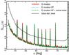 |
Fig. 6 Example |


Because for the baseline analysis we use high-pass filtered maps, we also show the analysis of the SMICAE-mode map high-pass filtered so that the lowest order multipoles (ℓ< 20) are removed from the map (the multipoles in the range 20 ≤ ℓ ≤ 40 are apodized between 0 and 1 using a cosine as defined in Planck Collaboration IX 2016). The high-pass filtering does not decrease our ability to detect a multiply-connected topology using the matched-circle method. This is consistent with the negligible sensitivity of the matched-circle statistic to the reionization signal, studied by Bielewicz et al. (2012). This is a consequence of the weighting of the polarization data by a factor proportional to ℓ2 employed in the transformation from the Stokes parameters Q and U to an E-mode map, which effectively filters out the largest-scale multipoles from the data. This test shows that the matched-circle method, contrary to the likelihood method, predominantly exploits the topological signal in the CMB anisotropies at moderate angular scales.
We also checked robustness of detection with respect to noise level in order to account for small discrepancies between the noise level in the Planck FFP8 simulations and the 2015 data (Planck Collaboration XII 2016). We repeated the analysis for the high-pass filtered map with added noise with 5% larger amplitude than for the original map. As we can see in Fig. 6, the statistic changes negligibly.
The intersection of the peaks in the matching statistic with the false detection level estimated for the CMB map corresponding to the simply-connected Universe defines the minimum radius of the correlated circles that can be detected for this map. We estimate the minimum radius by extrapolating the height of the peak with radius 18° seen in Fig. 6 towards smaller radii. This allows for a rough estimation of the radius, with a precision of a few degrees. However, better precision is not required, because for small minimum radius (as obtains here) constraints on the size of the fundamental domain are not very sensitive to differences of the minimum radius of order a few degrees. As we can see in Fig. 6, the minimum radius αmin takes a value in the range from 10° to around 15°. To be conservative we use the upper end of this range for the computation of constraints on the size of the fundamental domain, and we thus take αmin ≃ 15°.
Likelihood.
To validate and compare the performance of the two likelihood methods, we perform two sets of tests: a null test using a simulation of a simply connected Universe, and a signal test using a simulation of a toroidal Universe with  . The two test maps are generated at Nside = 16 and are band-limited using a 640′ Gaussian beam. Diagonal (white) noise is added with pixel variances
  and
and  , comparable to the expected eventual level of Planck’s 143 GHz channel. For clarity of interpretation, no mask is used in these tests; in this setting, the eigenmodes of the fiducial covariance matrix are linear combinations of the spherical harmonics at fixed wavenumber ℓ. As fully exploring the likelihood is much more time-consuming than profiling it, we generate a complete set of test results – analyses of the two test maps using cubic torus and slab covariance matrices on a fine grid of fundamental domain scales – using the profile-likelihood code, and aim to verify the main cubic torus results using the marginalized likelihood generated with AniCosmo. Note that to speed up the calculation of the marginalized likelihood we use a slightly smaller band-limit (ℓmax = 32) than in the profile-likelihood calculation (ℓmax = 40); with our choice of smoothing scale and mode count, and considering the full sky for validation purposes, we obtain the same eigenbasis (and therefore analyse the same projected data) in both cases.
The results for the null test – in the form of the likelihood function for the fundamental domain scale of the assumed topology – are plotted in Fig. 7 for cubic tori and Fig. 8 for slabs. Concentrating initially on the cubic tori, we see that the likelihoods derived from the two codes agree. In both cases, the likelihood is found to be maximal for fundamental domain scales larger than the horizon, and the small-L cubic tori are very strongly disfavoured:  . Note that the AniCosmo likelihood curve contains errors on the likelihood at each L considered, but these are orders of magnitude smaller than the changes in likelihood between points (typical MultiNest uncertainties yield errors of order 0.1 in log-likelihood).
In both cases, the profile likelihood exhibits a mild rise around the horizon scale, due to chance alignments along the matched faces of the fundamental domain. It is slightly stronger in the slab case since the probability of such alignments is greater with only a single pair of faces.
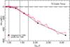 |
Fig. 7 Likelihood function for the fundamental domain scale of a cubic torus derived from simulations of a simply-connected Universe, calculated through marginalization (black, filled circles) and profiling (pink, empty circles). The horizontal axis gives the inverse of the length of a side of the fundamental domain, relative to the distance to the last-scattering surface. The vertical lines mark the positions where χrec is equal to various characteristic sizes of the fundamental domain, namely the radius of the largest sphere that can be inscribed in the domain, ℛi = L/ 2, the smallest sphere in which the domain can be inscribed, |


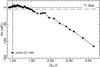 |
Fig. 8 Profile likelihood function for the fundamental domain scale of a slab topology derived from simulations of a simply-connected Universe. The vertical line marks the position where χrec is equal to the radius of the largest sphere that can be inscribed in the domain, ℛi = L/ 2 (for slab spaces, the other two characteristic sizes are infinite). |
The results for the tests on the toroidal simulation are shown in Fig. 9 for toroidal covariance matrices and Fig. 10 for slab covariance matrices. Concentrating first on the results employing toroidal covariance matrices, the correct fundamental domain scale is clearly picked out by both the profile and full likelihood codes, with the simply connected case strongly disfavoured at a likelihood ratio of  . Turning to the results derived using slab covariance matrices, we see that – as expected from the Kullback-Leibler divergence analysis of Sect. 3.1.2 – the correct fundamental domain scale is also found using the slab profile likelihood. Although, as also expected, the peak is not quite as pronounced when using the wrong covariance matrix, the simply connected Universe is still overwhelmingly disfavoured at a ratio of
  .
.
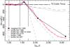 |
Fig. 9 Likelihood function for the fundamental domain scale of a cubic torus derived from a simulation of a toroidal Universe with |

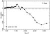 |
Fig. 10 Profile likelihood function for the fundamental domain scale of a slab derived from a simulation of a toroidal Universe with |
The speed of the profile-likelihood analysis allows for the effects of changing the mode count, composition, and noise level to be investigated. We repeat the toroidal test using intensity-only (I) and full (IQU) covariance matrices, retaining between 837 and 2170 modes at a time. For the smoothing scale employed in our tests, the 838th mode is the first to be dominated by polarization; runs using up to 837 IQU modes are therefore dominated by intensity information. The results of this investigation are contained in Fig. 9. The most striking conclusion is that the impact of adding temperature modes to the analysis is dwarfed by the impact of adding low-ℓ polarization information, even though the temperature modes are effectively noiseless. This conclusion is supported by the observation from Fig. 1 that the KL divergence grows most rapidly at low ℓ.
4.4.2. Bianchi
The Bayesian analysis of Bianchi VIIh models using temperature data is performed using the AniCosmo code, which has been extensively validated by McEwen et al. (2013), and was used to perform the Bianchi analysis of Planck Collaboration XXVI (2014). The maximum-likelihood template fitting method used to analyse polarization data is straightforward and has been validated on simulations, correctly recovering the amplitude of templates artificially embedded in simulated CMB observations.
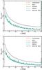 |
Fig. 11
|


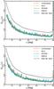 |
Fig. 12
|
5. Results
5.1. Topology
5.1.1. Matched circles
We show the matched-circle statistic for the CMB temperature and E-mode maps in Figs. 11 and 12, respectively. We do not find any statistically significant correlation of circle pairs in any map. Results for the temperature maps are consistent with the Planck Collaboration XXVI (2014) results. As discussed in Sect. 4.4.1, the minimum radius at which the peaks expected for the matching statistic are larger than the false detection level for the polarization map is around αmin ≃ 15°. Thus, we can exclude, at the confidence level of 99%, any topology that predicts matching pairs of back-to-back circles larger than this radius, assuming that the relative orientation of the fundamental domain and mask allows its detection. This implies that in a flat Universe described otherwise by the fiducial ΛCDM model, a 99% confidence-limit lower bound on the size of the fundamental domain is ℛi = L/ 2 ≳ χreccos(αmin) = 0.97 χrec or  . This is slightly stronger than the constraint obtained for the analysis of the 2013 Planck temperature maps, i.e., 0.94 χrec (Planck Collaboration XXVI 2014). Note that the limits from polarization are at least as strong as those from temperature despite the considerably smaller amount of sky considered in the polarization analysis (40% compared to 74%).
5.1.2. Likelihood
The results of applying the two likelihood codes to the Planck low-ℓ data are plotted in Fig. 13 for cubic tori and Fig. 14 for slabs. As with the null test, small-L topologies are strongly ruled out, and the likelihoods are maximized at scales approaching or exceeding the horizon. In the marginalized case, we find that the maximum-likelihood fundamental domain scale of a cubic torus is  , with scales of
  disfavoured at greater than 3.2 σ; for slabs, we find the likelihood to be peaked at
  (just inside the last-scattering surface), though is allowed at 1.9σ.
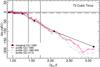 |
Fig. 13 Likelihood for the fundamental domain scale of a cubic torus derived from the Planck low-ℓ data set. As in testing, the likelihoods calculated via profiling (pink, clear circles) and marginalization (black, solid circles) agree well. The impact of increasing the polarization content through additional smoothing (purple, dashed) or modes (green, dot dashed) is diminished compared to the test setting due to boosted noise. |
We have investigated the shape of the likelihood as a function of the slab orientation, and find that it is strongly peaked at an orientation such that the induced matched circles lie partially within the large polarization mask (retaining only 47% of the sky). These orientations therefore do not benefit from the extra discriminatory power of the polarization and its correlation with temperature.
As noted when analysing simulations of simply-connected models (Figs. 7, 8), the profile likelihoods also show a mild rise around the horizon scale for the Planck data: this rise therefore cannot be interpreted as evidence for a multiply connected topology. We found a similar effect with both profile and marginalized likelihoods in Planck Collaboration XXVI (2014) using simulations of simply connected universes and the Planck temperature data, though this peak was considerably more pronounced for the profile likelihood. Further investigation is required to determine whether this extra-horizon rise is still present in the marginalized likelihood with the present data.
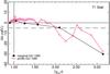 |
Fig. 14 Likelihood for the fundamental domain scale of a slab topology derived from the Planck low-ℓ data set via profiling (pink, clear circles) and marginalization (black, solid circles). |
Though the small-L topologies are strongly constrained by the data, we note that the dropoff in likelihood is not as sharp as that observed in our null test (or, indeed, the signal test) presented in Sect. 4.4.1. There are several reasons for this behaviour. The default smoothing scale used in the low-ℓPlanck data set (440′ Gaussian for intensity, no smoothing for polarization) means all of the first 1085 modes are in fact temperature-dominated. As our eigenbasis is constructed in decreasing-eigenvalue order, the greater the smoothing scale, the more small-scale temperature modes are damped in comparison to large-scale polarization modes, and thus the earlier polarization modes appear in the basis. Reducing the smoothing scale from 640′ (as used in testing) to 440′ (as used in the data) means the first polarization-dominated mode no longer appears in the 1085 highest-eigenvalue modes we take as our fiducial basis. Exploiting once more the speed of the profile likelihood code, we therefore explore the dependence of the likelihoods on the number of modes and their composition in Fig. 13. We introduce polarization-dominated eigenmodes into the analysis in two ways: by simply doubling the number of modes and by retaining the mode count but applying additional smoothing (to bring the effective Gaussian smoothing FWHM to 640′). Though the constraints on small-L topologies do become tighter when polarization-dominated modes are included, their impact remains weaker than in testing. This is because the noise in the low-ℓ data is significantly higher than in our tests – the typical diagonal covariance matrix element is  – and, finally, because we must use a sky cut, which can hide excess correlations. This strongly motivates repeating this analysis with the full multifrequency Planck polarization data when they become available.
Natural log-Bayes factors of Bianchi models relative to equivalent ΛCDM model (positive favours Bianchi model).
Converting these likelihoods into Bayesian constraints on the size of the fundamental domain is not straightforward. Absent a proper prior giving an upper limit on the size of the fundamental domain, there is always infinite parameter volume available for ever-larger fundamental domains. Hence, these likelihood plots should be considered the full summary of the 2015 Planck data for these models. Nonetheless, it is often useful to consider a fall-off in the likelihood of Δlnℒ < −5 as roughly equivalent to a 3σ–99% confidence level–limit, the location of which we approximate by interpolating between calculated likelihood points. For the cubic T3 torus, we find that the marginal likelihoods of the combined temperature and polarization lowT,P data require that the length of an edge of the fundamental domain satisfies  at this significance, or equivalently that the radius of the largest inscribed sphere in the fundamental domain is ℛi> 0.97 χrec (recall that is the comoving distance to the last-scattering surface.) The profile likelihood gives the somewhat weaker limit, ℛi> 0.79 χrec. For the T1 slab, we have
  or ℛi> 0.56 χrec. Because the temperature data on the relevant scales are still dominated by the cosmological signal, and the polarization noise remains large, these results are only slightly stronger than those presented in Planck Collaboration XXVI (2014).
5.2. Bianchi
Planck temperature data are masked and analysed for evidence of a Bianchi VIIh component, using the prior parameter ranges adopted in McEwen et al. (2013) and Planck Collaboration XXVI (2014). Cleaned temperature maps for each of the four component separation techniques are examined, where the mask defined for each technique is applied. The natural log-Bayes factors for the Bianchi models relative to their standard cosmological counterparts are shown in Table 1. The Bayes factors are broadly consistent across the component separation methods. Most Bayes factors are similar to the values computed in Planck Collaboration XXVI (2014), with the exception of the analysis of the left-handed flat-decoupled-Bianchi model with SEVEM data, which has increased, but which is now more consistent with the other component separation methods.
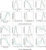 |
Fig. 15 Marginalized posterior distributions of Bianchi parameters recovered from PlanckSMICA (solid blue curves), SEVEM (dashed green curves), NILC (dot-dashed yellow curves), and Commander (dotted red curves) component-separated data for left-handed models. Planck data provide evidence in support of a Bianchi component in the phenomenological flat-decoupled-Bianchi model (panel a)) but not in the physical open-coupled-Bianchi model (panel b)). Significant differences exist between the posterior distributions shown in panel b) for each component separation method; this model is not favoured by data and parameters are in general poorly constrained. |
Parameters recovered for the left-handed flat-decoupled-Bianchi model.
For the phenomenological flat-decoupled-Bianchi model, evidence in support of a left-handed Bianchi template is again found (Table 1). The Bayes factors providing evidence for this model range between the values 2.3 ± 0.2 and 3.2 ± 0.2, corresponding to odds ratios of approximately 1:10 and 1:25, respectively (which on the Jeffreys scale are categorized as significant and strong, respectively; Jeffreys 1961). Recovered posterior distributions of the Bianchi parameters of this model for each component separation technique are shown in Fig. 15a. The posterior distributions are consistent across component separation techniques, are similar to those recovered in Planck Collaboration XXVI (2014), and are reasonably well constrained (with the exception of the known  –
– Bianchi parameter degeneracy Jaffe et al. 2006c; Bridges et al. 2007). Recall that the Bianchi densities ( and ) are decoupled from the standard cosmology in the flat-decoupled-Bianchi model considered here and, as found previously, are inconsistent with standard estimates of the densities. The maximum-a-posteriori (MAP) and mean-posterior Bianchi parameter estimates for this model are given in Table 2, while the corresponding MAP best-fit Bianchi temperature maps are shown in Fig. 16. Note that the maximum of a marginalized one-dimensional posterior (e.g., Fig. 15) will not in general coincide with the global MAP estimate for the full set of parameters. The best-fit maps for the left-handed flat-coupled-Bianchi model are consistent across component separation techniques and similar to the best-fit maps found in previous Planck (Planck Collaboration XXVI 2014) and WMAP (see, e.g., Jaffe et al. 2005; and McEwen et al. 2013) temperature data.
For the physical open-coupled-Bianchi model where the Bianchi VIIh model is coupled to the standard cosmology, there is again no evidence in support of a Bianchi contribution (Table 1). Recovered posterior distributions of the parameters of this model for each component separation technique are shown in Fig. 15b. The posterior distributions show some similarity across component separation techniques and with the distributions recovered in Planck Collaboration XXVI (2014). However, significant differences exist since the parameters are in general poorly constrained and the model is not favoured by the Bayesian evidence. The MAP and mean-posterior Bianchi parameter estimates for this model are given in Table 3, while the corresponding MAP best-fit Bianchi temperature maps are shown in Fig. 17. While the posterior distributions show differences between component separation techniques, the estimated parameters are consistent. Note that, although the mean parameter estimates have not changed markedly from Planck Collaboration XXVI (2014), the MAP estimates have indeed changed. Intriguingly, for each component separation technique, the MAP best-fit maps for the open-coupled-Bianchi model (Fig. 17), for which there is no evidence in support of a Bianchi contribution, show a similar but not identical morphology to the MAP best-fit maps for the flat-decoupled-Bianchi model (Fig. 16), for which the Bayesian evidence supports the inclusion of a Bianchi component. This was not the case in the previous Planck analysis (Planck Collaboration XXVI 2014, Fig. 22). A parameter combination is found for the physical open-coupled-Bianchi model that is broadly consistent with a standard open cosmology and that produces a Bianchi temperature map similar to the one found in the unphysical flat-decoupled-Bianchi model. This parameter combination lies on the known – Bianchi parameter degeneracy (Jaffe et al. 2006c; Bridges et al. 2007) and lies close to but not directly on the well-known CMB geometric degeneracy (determined by an independent CMB analysis), since both the cosmological and Bianchi components are fitted simultaneously. It is important to stress that Planck temperature data do not favour the physical open-coupled-Bianchi model, but neither is it possible to rule out this model using temperature data alone (Planck polarization data are considered subsequently). An overall constraint on the vorticity of Bianchi VIIh models, from Planck temperature data alone, of (ω/H)0< 7.6 × 10⁻¹⁰ (95% confidence level) is obtained from the analysis of the physical open-coupled-Bianchi model, which is consistent across all component separation techniques, as illustrated in Table 4.
To further constrain Bianchi VIIh models using Planck polarization data we simulate Bianchi polarization maps, computed using the approach of Pontzen & Challinor (2007) and Pontzen (2009), and provided by Pontzen (priv. comm.) for the best-fit Bianchi parameters determined from the temperature analysis. E- and B-mode Bianchi maps for the best-fit flat-decoupled-Bianchi model and the open-coupled-Bianchi model are displayed in Figs. 18 and 19, respectively. As described in Sect. 4.3.3, we estimate the maximum-likelihood amplitude of these Bianchi polarization templates in Planck polarization data, performing the analysis in the pixel space defined by the Q and U Stokes components, where noise and partial sky coverage can be handled effectively. The maximum-likelihood amplitudes estimated for each component separation technique are given in Table 5. The estimated amplitudes are close to zero and consistent across component separation techniques. The difference between the estimated amplitudes and zero is more likely due to small residual foreground contamination than a Bianchi component. Indeed, the amplitude estimates are at least 24 standard deviations from unity, the expected value for the best-fit Bianchi models determined from the temperature analysis. Both the best-fit flat-decoupled-Bianchi model and the open-decoupled-Bianchi model are thus strongly disfavoured by the Planck polarization data. This is not surprising since these models produce relatively strong E- and B-mode contributions (see Figs. 18 and 19), as highlighted already by Pontzen & Challinor (2007). However, the full freedom of Bianchi models remains to be explored using temperature and polarization data simultaneously, for example through a complete Bayesian analysis, which is left to future work.
Parameters recovered for the left-handed open-coupled-Bianchi model.
Upper bounds on vorticity (ω/H)0 at 95% confidence level.
Maximum-likelihood amplitude estimates λML and 1 σ errors computed using polarization data.
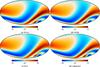 |
Fig. 16 Best-fit temperature maps for the left-handed flat-decoupled-Bianchi model. |
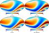 |
Fig. 17 Best-fit temperature maps for the left-handed open-coupled-Bianchi model. |
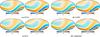 |
Fig. 18 Polarization maps for the best-fit left-handed flat-decoupled-Bianchi model fitted to temperature data. In each panel E- (left) and B-mode (right) maps are shown. These polarization maps are simulated using the approach of Pontzen & Challinor (2007) and Pontzen (2009), and provided by Pontzen (priv. comm.). |
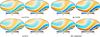 |
Fig. 19 Polarization maps for the best-fit left-handed open-coupled-Bianchi model fitted to temperature data. In each panel E- (left) and B-mode (right) maps are shown. These polarization maps are simulated using the approach of Pontzen & Challinor (2007) and Pontzen (2009), and provided by Pontzen (priv. comm.). |
6. Discussion
We have used Planck intensity and polarization data to evaluate specific departures from the large-scale isotropy of the Universe. Using both frequentist and Bayesian methods applied for the first time to polarization data, we find no evidence for a multi-connected topology with a scale less than roughly the distance to the last-scattering surface. Specifically, a frequentist search for antipodal matched circles on Nside = 512 maps finds a lower bound on the size of the fundamental domain of 0.97 χrec from polarization data alone. Using Bayesian methods applied to low-resolution (Nside = 16) maps of both temperature and polarization, we also find a lower limit of 0.97 χrec for the T3 cubic torus (for the T1 slab, the limit is 0.56 χrec). These results are both consistent and complementary, giving coincidentally identical limits but with very different statistical foundations and data selections. The addition of polarization data at current levels of accuracy does not significantly improve the limits from intensity alone, but we have found that the polarization sensitivity of the full set of Planck detectors should give quantitative improvements in the limits, decreasing the likelihood of fundamental domains with scales smaller than the distance to the last-scattering surface by many orders of magnitude.
We also find no evidence for a Bianchi VIIh model which departs from global isotropy via the presence of both rotation and shear. Although the large-scale temperature pattern measured by Planck has some similar features to that induced by focusing in a Bianchi VIIh Universe, it requires unphysical parameters. Fixed to those parameters, we have further shown that the polarization pattern induced by such models is strongly disfavoured by the Planck data.
The results outlined here show no evidence for departures from isotropic and simply-connected models. Improved computational techniques, along with future polarization data from Planck (and beyond), will allow yet stronger checks of even wider classes of models. For the multi-connected case, we can expand to models without antipodal matched circles and with the scale of the fundamental domain closer to (and even slightly beyond) the last-scattering surface. For the likelihood method, this will require computation of the correlation matrix with higher-wavenumber modes to capture more of the available information.
For anisotropic models, we can explicitly perform parameter estimation and model selection using polarization data, beyond the simple template-fitting performed here.
Although the evidence thus far corroborates the conventional wisdom that we live in the simplest FLRW Universe, this is likely to be only an approximation vastly beyond the Hubble scale. Detection of a multiply-connected topology or anisotropic geometry is one of the few ways to probe the global structure of spacetime. We have shown that Planck data give the best handle to date on these possibilities.
Planck (http://www.esa.int/Planck) is a project of the European Space Agency (ESA) with instruments provided by two scientific consortia funded by ESA member states and led by Principal Investigators from France and Italy, telescope reflectors provided through a collaboration between ESA and a scientific consortium led and funded by Denmark, and additional contributions from NASA (USA).
The active zyz Euler convention is adopted, corresponding to the rotation of a physical body in a fixed coordinate system about the z, y, and z axes by γ, β, and α, respectively.
Acknowledgments
The Planck Collaboration acknowledges the support of: ESA; CNES and CNRS/INSU-IN2P3-INP (France); ASI, CNR, and INAF (Italy); NASA and DoE (USA); STFC and UKSA (UK); CSIC, MINECO, JA, and RES (Spain); Tekes, AoF, and CSC (Finland); DLR and MPG (Germany); CSA (Canada); DTU Space (Denmark); SER/SSO (Switzerland); RCN (Norway); SFI (Ireland); FCT/MCTES (Portugal); ERC and PRACE (EU). A description of the Planck Collaboration and a list of its members, indicating which technical or scientific activities they have been involved in, can be found at http://www.cosmos.esa.int/web/planck/planck-collaboration. The authors thank Andrew Pontzen for computing Bianchi VIIh polarization templates for the best-fit models resulting from the analysis of temperature data. We acknowledge the UCL Legion High Performance Computing Facility (Legion@UCL) and associated support services in the completion of this work. Parts of the computations were performed on the Andromeda and Perseus clusters of the University of Geneva, as well as the Carver IBM iDataPlex, the Hopper Cray XE6, and the Edison Cray XC30 at NERSC, and on the GPC supercomputer at the SciNet HPC Consortium. SciNet is funded by: the Canada Foundation for Innovation under the auspices of Compute Canada; the Government of Ontario; Ontario Research Fund − Research Excellence; and the University of Toronto.
References
- Aurich, R. 1999, ApJ, 524, 497 [NASA ADS] [CrossRef] [Google Scholar]
- Aurich, R., & Lustig, S. 2013, MNRAS, 433, 2517 [NASA ADS] [CrossRef] [Google Scholar]
- Aurich, R., & Lustig, S. 2014, Class. Quant. Grav., 31, 165009 [NASA ADS] [CrossRef] [Google Scholar]
- Aurich, R., Lustig, S., Steiner, F., & Then, H. 2004, Class. Quant. Grav., 21, 4901 [NASA ADS] [CrossRef] [Google Scholar]
- Aurich, R., Lustig, S., & Steiner, F. 2005, Class. Quant. Grav., 22, 2061 [Google Scholar]
- Aurich, R., Lustig, S., & Steiner, F. 2006, MNRAS, 369, 240 [NASA ADS] [CrossRef] [Google Scholar]
- Aurich, R., Janzer, H. S., Lustig, S., & Steiner, F. 2008, Class. Quant. Grav., 25, 125006 [NASA ADS] [CrossRef] [Google Scholar]
- Barrow, J. D. 1986, Can. J. Phys., 64, 152 [NASA ADS] [CrossRef] [Google Scholar]
- Barrow, J. D., Juszkiewicz, R., & Sonoda, D. H. 1985, MNRAS, 213, 917 [NASA ADS] [CrossRef] [Google Scholar]
- Bennett, C. L., Banday, A. J., Gorski, K. M., et al. 1996, ApJ, 464, L1 [NASA ADS] [CrossRef] [Google Scholar]
- Bielewicz, P., & Banday, A. J. 2011, MNRAS, 412, 2104 [NASA ADS] [CrossRef] [Google Scholar]
- Bielewicz, P., & Riazuelo, A. 2009, MNRAS, 396, 609 [NASA ADS] [CrossRef] [Google Scholar]
- Bielewicz, P., Banday, A. J., & Górski, K. M. 2012, MNRAS, 421, 1064 [NASA ADS] [CrossRef] [Google Scholar]
- Bond, J. R., & Efstathiou, G. 1987, MNRAS, 226, 655 [NASA ADS] [Google Scholar]
- Bond, J. R., Jaffe, A. H., & Knox, L. E. 1998a, Phys. Rev. D, 57, 2117 [NASA ADS] [CrossRef] [Google Scholar]
- Bond, J. R., Pogosyan, D., & Souradeep, T. 1998b, Class. Quant. Grav., 15, 2671 [NASA ADS] [CrossRef] [Google Scholar]
- Bond, J. R., Pogosyan, D., & Souradeep, T. 2000, Phys. Rev. D, 62, 043006 [NASA ADS] [CrossRef] [Google Scholar]
- Bridges, M., McEwen, J. D., Lasenby, A. N., & Hobson, M. P. 2007, MNRAS, 377, 1473 [NASA ADS] [CrossRef] [MathSciNet] [Google Scholar]
- Bridges, M., McEwen, J. D., Cruz, M., et al. 2008, MNRAS, 390, 1372 [NASA ADS] [Google Scholar]
- Bunn, E. F., Ferreira, P. G., & Silk, J. 1996, Phys. Lett., 77, 2883 [Google Scholar]
- Caillerie, S., Lachièze-Rey, M., Luminet, J.-P., et al. 2007, A&A, 476, 691 [NASA ADS] [CrossRef] [EDP Sciences] [Google Scholar]
- Cayón, L., Banday, A. J., Jaffe, T., et al. 2006, MNRAS, 369, 598 [NASA ADS] [CrossRef] [Google Scholar]
- Collins, C. B., & Hawking, S. W. 1973, MNRAS, 162, 307 [NASA ADS] [CrossRef] [Google Scholar]
- Cornish, N. J., Spergel, D. N., & Starkman, G. D. 1998, Class. Quant. Grav., 15, 2657 [Google Scholar]
- Cornish, N. J., Spergel, D. N., Starkman, G. D., & Komatsu, E. 2004, Phys. Rev. Lett., 92, 201302 [NASA ADS] [CrossRef] [PubMed] [Google Scholar]
- de Oliveira-Costa, A., & Smoot, G. F. 1995, ApJ, 448, 477 [NASA ADS] [CrossRef] [Google Scholar]
- Dineen, P., Rocha, G., & Coles, P. 2005, MNRAS, 358, 1285 [NASA ADS] [CrossRef] [Google Scholar]
- Fagundes, H. V., & Wichoski, U. F. 1987, Nature, 322, L5 [Google Scholar]
- Fang, L.-Z., & Sato, H. 1983, Commun. Theor. Phys., 2, 1055 [Google Scholar]
- Feroz, F., & Hobson, M. P. 2008, MNRAS, 384, 449 [NASA ADS] [CrossRef] [Google Scholar]
- Feroz, F., Hobson, M. P., & Bridges, M. 2009, MNRAS, 398, 1601 [NASA ADS] [CrossRef] [Google Scholar]
- Feroz, F., Hobson, M. P., Cameron, E., & Pettitt, A. N. 2013, ArXiv e-prints [arXiv:1306.2144] [Google Scholar]
- Fujii, H., & Yoshii, Y. 2011, A&A, 529, A121 [NASA ADS] [CrossRef] [EDP Sciences] [Google Scholar]
- Ghosh, T., Hajian, A., & Souradeep, T. 2007, Phys. Rev. D, 75, 083007 [Google Scholar]
- Jaffe, T. R., Banday, A. J., Eriksen, H. K., Górski, K. M., & Hansen, F. K. 2005, ApJ, 629, L1 [NASA ADS] [CrossRef] [Google Scholar]
- Jaffe, T. R., Banday, A. J., Eriksen, H. K., Górski, K. M., & Hansen, F. K. 2006a, A&A, 460, 393 [NASA ADS] [CrossRef] [EDP Sciences] [Google Scholar]
- Jaffe, T. R., Banday, A. J., Eriksen, H. K., Górski, K. M., & Hansen, F. K. 2006b, ApJ, 643, 616 [NASA ADS] [CrossRef] [Google Scholar]
- Jaffe, T. R., Hervik, S., Banday, A. J., & Górski, K. M. 2006c, ApJ, 644, 701 [NASA ADS] [CrossRef] [Google Scholar]
- Jarosik, N., Bennett, C. L., Dunkley, J., et al. 2011, ApJS, 192, 14 [NASA ADS] [CrossRef] [Google Scholar]
- Jeffreys, H. 1961, Theory of probability, 3rd edn. (Oxford: Oxford University Press) [Google Scholar]
- Key, J. S., Cornish, N. J., Spergel, D. N., & Starkman, G. D. 2007, Phys. Rev. D, 75, 084034 [NASA ADS] [CrossRef] [Google Scholar]
- Kim, J. 2011, A&A, 531, A32 [NASA ADS] [CrossRef] [EDP Sciences] [Google Scholar]
- Kogut, A., Hinshaw, G., & Banday, A. J. 1997, Phys. Rev. D, 55, 1901 [NASA ADS] [CrossRef] [Google Scholar]
- Kosowsky, A. 1996, Ann. Phys., 246, 49 [NASA ADS] [CrossRef] [Google Scholar]
- Kunz, M., Aghanim, N., Cayon, L., et al. 2006, Phys. Rev. D, D73, 023511 [NASA ADS] [CrossRef] [Google Scholar]
- Kunz, M., Aghanim, N., Riazuelo, A., & Forni, O. 2008, Phys. Rev. D, 77, 23525 [Google Scholar]
- Lachieze-Rey, M., & Luminet, J. 1995, Phys. Rep., 254, 135 [NASA ADS] [CrossRef] [Google Scholar]
- Land, K., & Magueijo, J. 2006, MNRAS, 367, 1714 [NASA ADS] [CrossRef] [Google Scholar]
- Lehoucq, R., Lachieze-Rey, M., & Luminet, J. P. 1996, A&A, 313, 339 [NASA ADS] [Google Scholar]
- Levin, J. 2002, Phys. Rep., 365, 251 [NASA ADS] [CrossRef] [Google Scholar]
- Levin, J., Scannapieco, E., & Silk, J. 1998, Nature, 58, 103516 [Google Scholar]
- Lew, B., & Roukema, B. 2008, A&A, 482, 747 [NASA ADS] [CrossRef] [EDP Sciences] [Google Scholar]
- Luminet, J.-P., Weeks, J. R., Riazuelo, A., Lehoucq, R., & Uzan, J.-P. 2003, Nature, 425, 593 [NASA ADS] [CrossRef] [PubMed] [Google Scholar]
- McEwen, J. D., Hobson, M. P., Lasenby, A. N., & Mortlock, D. J. 2006, MNRAS, 369, 1858 [NASA ADS] [CrossRef] [Google Scholar]
- McEwen, J. D., Josset, T., Feeney, S. M., Peiris, H. V., & Lasenby, A. N. 2013, MNRAS, 436, 3680 [NASA ADS] [CrossRef] [Google Scholar]
- Niarchou, A., & Jaffe, A. H. 2007, Phys. Rev. Lett., 99, 81302 [Google Scholar]
- Niarchou, A., Jaffe, A. H., & Pogosian, L. 2004, Phys. Rev. D, 69, 063515 [Google Scholar]
- Phillips, N. G., & Kogut, A. 2006, ApJ, 645, 820 [NASA ADS] [CrossRef] [Google Scholar]
- Planck Collaboration XXVI. 2014, A&A, 571, A26 [NASA ADS] [CrossRef] [EDP Sciences] [Google Scholar]
- Planck Collaboration I. 2016, A&A, 594, A1 [NASA ADS] [CrossRef] [EDP Sciences] [Google Scholar]
- Planck Collaboration II. 2016, A&A, 594, A2 [NASA ADS] [CrossRef] [EDP Sciences] [Google Scholar]
- Planck Collaboration III. 2016, A&A, 594, A3 [NASA ADS] [CrossRef] [EDP Sciences] [Google Scholar]
- Planck Collaboration IV. 2016, A&A, 594, A4 [NASA ADS] [CrossRef] [EDP Sciences] [Google Scholar]
- Planck Collaboration V. 2016, A&A, 594, A5 [NASA ADS] [CrossRef] [EDP Sciences] [Google Scholar]
- Planck Collaboration VI. 2016, A&A, 594, A6 [NASA ADS] [CrossRef] [EDP Sciences] [Google Scholar]
- Planck Collaboration VII. 2016, A&A, 594, A7 [NASA ADS] [CrossRef] [EDP Sciences] [Google Scholar]
- Planck Collaboration VIII. 2016, A&A, 594, A8 [NASA ADS] [CrossRef] [EDP Sciences] [Google Scholar]
- Planck Collaboration IX. 2016, A&A, 594, A9 [NASA ADS] [CrossRef] [EDP Sciences] [Google Scholar]
- Planck Collaboration X. 2016, A&A, 594, A10 [NASA ADS] [CrossRef] [EDP Sciences] [Google Scholar]
- Planck Collaboration XI. 2016, A&A, 594, A11 [NASA ADS] [CrossRef] [EDP Sciences] [Google Scholar]
- Planck Collaboration XII. 2016, A&A, 594, A12 [NASA ADS] [CrossRef] [EDP Sciences] [Google Scholar]
- Planck Collaboration XIII. 2016, A&A, 594, A13 [NASA ADS] [CrossRef] [EDP Sciences] [Google Scholar]
- Planck Collaboration XIV. 2016, A&A, 594, A14 [NASA ADS] [CrossRef] [EDP Sciences] [Google Scholar]
- Planck Collaboration XV. 2016, A&A, 594, A15 [NASA ADS] [CrossRef] [EDP Sciences] [Google Scholar]
- Planck Collaboration XVI. 2016, A&A, 594, A16 [NASA ADS] [CrossRef] [EDP Sciences] [Google Scholar]
- Planck Collaboration XVII. 2016, A&A, 594, A17 [NASA ADS] [CrossRef] [EDP Sciences] [Google Scholar]
- Planck Collaboration XVIII. 2016, A&A, 594, A18 [NASA ADS] [CrossRef] [EDP Sciences] [Google Scholar]
- Planck Collaboration XIX. 2016, A&A, 594, A19 [NASA ADS] [CrossRef] [EDP Sciences] [Google Scholar]
- Planck Collaboration XX. 2016, A&A, 594, A20 [NASA ADS] [CrossRef] [EDP Sciences] [Google Scholar]
- Planck Collaboration XXI. 2016, A&A, 594, A21 [NASA ADS] [CrossRef] [EDP Sciences] [Google Scholar]
- Planck Collaboration XXII. 2016, A&A, 594, A22 [NASA ADS] [CrossRef] [EDP Sciences] [Google Scholar]
- Planck Collaboration XXIII. 2016, A&A, 594, A23 [NASA ADS] [CrossRef] [EDP Sciences] [Google Scholar]
- Planck Collaboration XXIV. 2016, A&A, 594, A24 [NASA ADS] [CrossRef] [EDP Sciences] [Google Scholar]
- Planck Collaboration XXV. 2016, A&A, 594, A25 [NASA ADS] [CrossRef] [EDP Sciences] [Google Scholar]
- Planck Collaboration XXVI. 2016, A&A, 594, A26 [NASA ADS] [CrossRef] [EDP Sciences] [Google Scholar]
- Planck Collaboration XXVII. 2016, A&A, 594, A27 [NASA ADS] [CrossRef] [EDP Sciences] [Google Scholar]
- Planck Collaboration XXVIII. 2016, A&A, 594, A28 [NASA ADS] [CrossRef] [EDP Sciences] [Google Scholar]
- Pontzen, A. 2009, Phys. Rev. D, 79, 103518 [NASA ADS] [CrossRef] [Google Scholar]
- Pontzen, A., & Challinor, A. 2007, MNRAS, 380, 1387 [NASA ADS] [CrossRef] [Google Scholar]
- Pontzen, A., & Challinor, A. 2011, Class. Quant. Grav., 28, 185007 [NASA ADS] [CrossRef] [Google Scholar]
- Press, W. H., Teukolsky, S. A., Vetterling, W. T., & Flannery, B. P. 1992, Numerical Recipes in C: The Art of Scientific Computing, 2nd edn. (New York, NY, USA: Cambridge University Press) [Google Scholar]
- Riazuelo, A., Uzan, J.-P., Lehoucq, R., & Weeks, J. 2004a, Phys. Rev. D, 69, 103514 [NASA ADS] [CrossRef] [Google Scholar]
- Riazuelo, A., Weeks, J., Uzan, J.-P., Lehoucq, R., & Luminet, J.-P. 2004b, Phys. Rev. D, 69, 103518 [NASA ADS] [CrossRef] [Google Scholar]
- Riazuelo, A., Caillerie, S., Lachièze-Rey, M., Lehoucq, R., & Luminet, J.-P. 2006, ArXiv e-prints [arXiv:astro-ph/0601433] [Google Scholar]
- Rocha, G., Cayón, L., Bowen, R., et al. 2004, MNRAS, 351, 769 [NASA ADS] [CrossRef] [Google Scholar]
- Roukema, B. F. 1996, MNRAS, 283, 1147 [NASA ADS] [Google Scholar]
- Roukema, B. F. 2000a, Class. Quant. Grav., 17, 3951 [NASA ADS] [CrossRef] [Google Scholar]
- Roukema, B. F. 2000b, MNRAS, 312, 712 [NASA ADS] [CrossRef] [Google Scholar]
- Roukema, B. F., Buliński, Z., & Gaudin, N. E. 2008, A&A, 492, 657 [Google Scholar]
- Seljak, U., & Zaldarriaga, M. 1996, ApJ, 469, 437 [NASA ADS] [CrossRef] [Google Scholar]
- Skilling, J. 2004, in AIP Conf. Ser. 735, eds. R. Fischer, R. Preuss, & U. V. Toussaint, 395 [Google Scholar]
- Sokolov, I. Y. 1993, Sov. J. Exp. Theor. Phys. Lett., 57, 617 [Google Scholar]
- Sokolov, D. D., & Shvartsman, V. F. 1974, Sov. J. Exp. Theor. Phys., 39, 196 [Google Scholar]
- Starobinskij, A. A. 1993, Sov. J. Exp. Theor. Phys. Lett., 57, 622 [Google Scholar]
- Stevens, D., Scott, D., & Silk, J. 1993, Phys. Rev. Lett., 71, 20 [NASA ADS] [CrossRef] [Google Scholar]
- Vaudrevange, P. M., Starkman, G. D., Cornish, N. J., & Spergel, D. N. 2012, Phys. Rev. D, 86, 083526 [NASA ADS] [CrossRef] [Google Scholar]
- Weatherley, S. J., Warren, S. J., Croom, S. M., et al. 2003, Nature, 342, L9 [Google Scholar]
All Tables
Natural log-Bayes factors of Bianchi models relative to equivalent ΛCDM model (positive favours Bianchi model).
Maximum-likelihood amplitude estimates λML and 1 σ errors computed using polarization data.
All Figures
|
Fig. 1 KL divergence of slab (T1) topologies relative to an infinite Universe as a function of ℓmax with sizes |
| In the text | |
|
Fig. 2 KL divergence of fixed cubic, rod, and slab topologies with fundamental domain side |
| In the text | |
|
Fig. 3 KL divergence of a slab space relative to a cubic topology, as a function of rotation angle of the slab space (blue curve). Both spaces have |
| In the text | |
|
Fig. 4 Mode structure plotted as maps for the eigenvector corresponding to the highest-signal eigenvalue of the fiducial simply-connected model. The top map corresponds to temperature, middle to Q polarization, and bottom to U polarization. Masked pixels are plotted in grey. |
| In the text | |
|
Fig. 5 Mode structure plotted as maps for the eigenvector corresponding to the 301st-highest-signal eigenvalue of the fiducial simply-connected model. The top map corresponds to temperature, middle to Q polarization, and bottom to U polarization. Masked pixels are plotted in grey. |
| In the text | |
|
Fig. 6 Example |
| In the text | |
|
Fig. 7 Likelihood function for the fundamental domain scale of a cubic torus derived from simulations of a simply-connected Universe, calculated through marginalization (black, filled circles) and profiling (pink, empty circles). The horizontal axis gives the inverse of the length of a side of the fundamental domain, relative to the distance to the last-scattering surface. The vertical lines mark the positions where χrec is equal to various characteristic sizes of the fundamental domain, namely the radius of the largest sphere that can be inscribed in the domain, ℛi = L/ 2, the smallest sphere in which the domain can be inscribed, |
| In the text | |
|
Fig. 8 Profile likelihood function for the fundamental domain scale of a slab topology derived from simulations of a simply-connected Universe. The vertical line marks the position where χrec is equal to the radius of the largest sphere that can be inscribed in the domain, ℛi = L/ 2 (for slab spaces, the other two characteristic sizes are infinite). |
| In the text | |
|
Fig. 9 Likelihood function for the fundamental domain scale of a cubic torus derived from a simulation of a toroidal Universe with |
| In the text | |
|
Fig. 10 Profile likelihood function for the fundamental domain scale of a slab derived from a simulation of a toroidal Universe with |
| In the text | |
|
Fig. 11
|
| In the text | |
|
Fig. 12
|
| In the text | |
|
Fig. 13 Likelihood for the fundamental domain scale of a cubic torus derived from the Planck low-ℓ data set. As in testing, the likelihoods calculated via profiling (pink, clear circles) and marginalization (black, solid circles) agree well. The impact of increasing the polarization content through additional smoothing (purple, dashed) or modes (green, dot dashed) is diminished compared to the test setting due to boosted noise. |
| In the text | |
|
Fig. 14 Likelihood for the fundamental domain scale of a slab topology derived from the Planck low-ℓ data set via profiling (pink, clear circles) and marginalization (black, solid circles). |
| In the text | |
|
Fig. 15 Marginalized posterior distributions of Bianchi parameters recovered from PlanckSMICA (solid blue curves), SEVEM (dashed green curves), NILC (dot-dashed yellow curves), and Commander (dotted red curves) component-separated data for left-handed models. Planck data provide evidence in support of a Bianchi component in the phenomenological flat-decoupled-Bianchi model (panel a)) but not in the physical open-coupled-Bianchi model (panel b)). Significant differences exist between the posterior distributions shown in panel b) for each component separation method; this model is not favoured by data and parameters are in general poorly constrained. |
| In the text | |
|
Fig. 16 Best-fit temperature maps for the left-handed flat-decoupled-Bianchi model. |
| In the text | |
|
Fig. 17 Best-fit temperature maps for the left-handed open-coupled-Bianchi model. |
| In the text | |
|
Fig. 18 Polarization maps for the best-fit left-handed flat-decoupled-Bianchi model fitted to temperature data. In each panel E- (left) and B-mode (right) maps are shown. These polarization maps are simulated using the approach of Pontzen & Challinor (2007) and Pontzen (2009), and provided by Pontzen (priv. comm.). |
| In the text | |
|
Fig. 19 Polarization maps for the best-fit left-handed open-coupled-Bianchi model fitted to temperature data. In each panel E- (left) and B-mode (right) maps are shown. These polarization maps are simulated using the approach of Pontzen & Challinor (2007) and Pontzen (2009), and provided by Pontzen (priv. comm.). |
| In the text | |
Current usage metrics show cumulative count of Article Views (full-text article views including HTML views, PDF and ePub downloads, according to the available data) and Abstracts Views on Vision4Press platform.
Data correspond to usage on the plateform after 2015. The current usage metrics is available 48-96 hours after online publication and is updated daily on week days.
Initial download of the metrics may take a while.