| Issue |
A&A
Volume 589, May 2016
|
|
|---|---|---|
| Article Number | A116 | |
| Number of page(s) | 26 | |
| Section | Galactic structure, stellar clusters and populations | |
| DOI | https://doi.org/10.1051/0004-6361/201527554 | |
| Published online | 21 April 2016 | |
Multiwavelength study of the flaring activity of Sagittarius A in 2014 February−April⋆
1
Observatoire astronomique de Strasbourg, Université de Strasbourg, CNRS,
UMR 7550, 11 rue de
l’Université, 67000
Strasbourg, France
e-mail: This email address is being protected from spambots. You need JavaScript enabled to view it.
2
Space Telescope Science Institute (STScI),
3700 San Martin Drive,
Baltimore, MD
21218,
USA
3 Physikalisches Institut der
Universität zu Köln, Zülpicher Str.
77, 50937
Köln,
Germany
4
Max-Planck-Institut für Radioastronomie,
Auf dem Hügel 69, 53121
Bonn,
Germany
5
Department of Physics and Astronomy, CIERA, Northwestern
University, Evanston,
IL
60208,
USA
6
Radio Astronomy Laboratory, University of
California, Berkeley,
CA
94720,
USA
7
National Radio Astronomy Observatory, Charlottesville, VA
22903,
USA
Received: 14 October 2015
Accepted: 1 March 2016
Abstract
Context. The supermassive black hole named Sgr A* is located at the dynamical center of the Milky Way. This closest supermassive black hole is known to have a luminosity several orders of magnitude lower than the Eddington luminosity. Flares coming from the Sgr A* environment can be observed in infrared, X-ray, and submillimeter wavelengths, but their origins are still debated. Interestingly, the close passage of the Dusty S-cluster Object (DSO)/G2 near Sgr A* may increase the black hole flaring activity and could therefore help us to better constrain the radiation mechanisms from Sgr A*.
Aims. Our aim is to study the X-ray, infrared, and radio flaring activity of Sgr A* close to the time of the DSO/G2 pericenter passage in order to constrain the physical properties and origin of the flares.
Methods. Simultaneous observations were made with XMM-Newton and WFC3 onboard HST during the period Feb.–Apr. 2014, in addition to coordinated observations with SINFONI at ESO’s VLT, VLA in its A-configuration, and CARMA.
Results. We detected two X-ray flares on 2014 Mar. 10 and Apr. 2 with XMM-Newton, three near-infrared (NIR) flares with HST on 2014 Mar. 10 and Apr. 2, and two NIR flares on 2014 Apr. 3 and 4 with VLT. The X-ray flare on 2014 Mar. 10 is characterized by a long rise (~7700 s) and a rapid decay (~844 s). Its total duration is one of the longest detected so far in X-rays. Its NIR counterpart peaked well before (4320 s) the X-ray maximum, implying a dramatic change in the X-ray-to-NIR flux ratio during this event. This NIR/X-ray flare is interpreted as either a single flare where variation in the X-ray-to-NIR flux ratio is explained by the adiabatic compression of a plasmon, or two distinct flaring components separated by 1.2 h with simultaneous peaks in X-rays and NIR. We identified an increase in the rising radio flux density at 13.37 GHz on 2014 Mar. 10 with the VLA that could be the delayed radio emission from a NIR/X-ray flare that occurred before the start of our observation. The X-ray flare on 2014 Apr. 2 occurred for HST during the occultation of Sgr A* by the Earth, therefore we only observed the start of its NIR counterpart. With NIR synchrotron emission from accelerated electrons and assuming X-rays from synchrotron self-Compton emission, the region of this NIR/X-ray flare has a size of 0.03−7 times the Schwarzschild radius and an electron density of 108.5–1010.2 cm-3, assuming a synchrotron spectral index of 0.3−1.5. When Sgr A* reappeared to the HST view, we observed the decay phase of a distinct bright NIR flare with no detectable counterpart in X-rays. On 2014 Apr. 3, two 3.2-mm flares were observed with CARMA, where the first may be the delayed (4.4 h) emission of a NIR flare observed with VLT.
Conclusions. We observed a total of seven NIR flares, with three having a detected X-ray counterpart. The physical parameters of the flaring region are less constrained for the NIR flare without a detected X-ray counterpart, but none of the possible radiative processes (synchrotron, synchrotron self-Compton, or inverse Compton) can be ruled out for the production of the X-ray flares. The three X-ray flares were observed during the XMM-Newton total effective exposure of ~256 ks. This flaring rate is statistically consistent with those observed during the 2012 Chandra XVP campaign, implying that no increase in the flaring activity was triggered close to the pericenter passage of the DSO/G2. Moreover, higher flaring rates had already been observed with Chandra and XMM-Newton without any increase in the quiescent level, showing that there is no direct link between an increase in the flaring rate in X-rays and the change in the accretion rate.
Key words: Galaxy: center / X-rays: individuals: Sgr A* / radiation mechanisms: general
The tables of the data used for the light curves are only available at the CDS via anonymous ftp to cdsarc.u-strasbg.fr (130.79.128.5) or via http://cdsarc.u-strasbg.fr/viz-bin/qcat?J/A+A/589/A116
© ESO, 2016
1. Introduction
Sgr A*, located at the dynamical center of our Galaxy, is currently a dormant supermassive black hole (SMBH) of mass M about 4 × 10⁶M⊙ (Schödel et al. 2002; Ghez et al. 2008; Gillessen et al. 2009). Its bolometric luminosity (Lbol ~ 1036 erg s-1) is lower than the Eddington luminosity (LEdd = 3.3 × 10⁴M/M⊙L⊙ = 3 × 1044 erg s-1) (Yuan et al. 2003). This low luminosity can be explained by radiatively inefficient accretion flow models (RIAF) such as advection-dominated accretion flows (ADAF; Narayan et al. 1998) and jet-disk models. Because of its proximity (d = 8 kpc; Genzel et al. 2010; Falcke & Markoff 2013), Sgr A* is the best target to study the accretion and ejection physics for the case of low accretion rate, which is a regime where SMBH’s are supposed to spend most of their lifetime. Its physical understanding can be applied to a large number of normal galaxies that are supposed to host a SMBH.
Above Sgr A* quiescent emission, some episodes of increased flux are observed in X-rays, near-infrared (NIR), and sub-millimeter/radio. These flaring events from Sgr A* were first discovered in X-rays (Baganoff et al. 2001) and were then also observed in NIR (Genzel et al. 2003) and sub-millimeter wavelengths (Zhao 2003). NIR flares, which happen several times per day and have various amplitude up to 32 mJy (Witzel et al. 2012), are interpreted as synchrotron emission from accelerated electrons close to the black hole (Eisenhauer et al. 2005; Eckart et al. 2006). In the NIR, the synchrotron emission is optically thick and the spectral index between the H and L band is α = −0.62 ± 0.1 with Sν ∝ να (Witzel et al. 2014b). The X-ray flaring rate is 1.0−1.3 flares per day (Neilsen et al. 2013), but two episodes of higher flaring activity in X-rays have been observed (Porquet et al. 2008; Neilsen et al. 2013). Most X-ray flares have moderate amplitude (Neilsen et al. 2013) with 2–45 times the quiescent luminosity of Sgr A* (about 3.6 × 1033 erg s-1 in 2−8 keV; Baganoff et al. 2003; Nowak et al. 2012), but brighter flares with amplitudes up to 160 times the quiescent level have also been observed (Porquet et al. 2003, 2008; Nowak et al. 2012). Several emission mechanism models are proposed in order to explain X-ray flares, such as: synchrotron (Dodds-Eden et al. 2009; Barrière et al. 2014), synchrotron self-Compton (Eckart et al. 2008), and inverse Compton (Yusef-Zadeh et al. 2006b; Wardle 2011; Yusef-Zadeh et al. 2012) emissions. During simultaneous NIR/X-ray observations, X-ray flares always have a NIR counterpart and their light curves have similar shapes, with an apparent delay less than 3 min between the peaks of flare emission (Eckart et al. 2006; Yusef-Zadeh et al. 2006a; Dodds-Eden et al. 2009). The sub-millimeter and radio flare peaks, however, are delayed several tens of minutes and hours, respectively (Marrone et al. 2008; Yusef-Zadeh et al. 2008, 2009), and are proposed to be due to synchrotron radiation of an expanding relativistic plasma blob with an adiabatic cooling (Yusef-Zadeh et al. 2006a). Considering the intrinsic size of Sgr A* at a wavelength λ of (0.52 ± 0.03) mas × (λ/ cm)1.3 ± 0.1, the time lag between the sub-millimeter and radio light curves suggests a collimated outflow (Brinkerink et al. 2015). On 2012 May 17, a NIR flare was followed 4.5 ± 0.5 h later by a 7-mm flare that was observed with the Very Long Baseline Array (VLBA) and localized 1.5 mas southeast of Sgr A*, providing evidence for an adiabatically expanding jet with a speed of 0.4 ± 0.3c (Rauch et al. 2016).
Gillessen et al. (2012) reported the detection of the object named G2 on its way towards Sgr A* in an eccentric Keplerian orbit with the 2004 data from the Very Large Telescope (VLT) using the Spectrograph for INtegral Field Observations in the Near-Infrared (SINFONI) and the Nasmyth Adaptive Optics System (NAOS) and COudé Near-IR Camera (CONICA), i.e., NACO. Their observations of the redshifted emission lines Brγ, Brδ, and HeI in the NIR between 2004 and 2011 allowed them to determine the pericenter passage of 2013.51 ± 0.04. They developed the first interpretation of the nature of the G2 object based on the observation of these lines: a compact gas blob. From the M-band they showed that G2 has a dust temperature consistent with 450 K. They predicted that, because G2 moves supersonically through the ambient hot gas, a bow shock should be created close to the pericenter passagei, which should be seen from radio to X-rays. The observation of such X-ray emission could help to put some constraints on the physical characteristics of the ambient medium around Sgr A*. The compact gas blob interpretation was still favored by Gillessen et al. (2013a) who analyzed the Brγ line width using data from SINFONI and NACO in March−July 2012. They derived a pericenter passage of 2013.69 ± 0.04, adding their observations to those between 2004 and 2011. A velocity-position diagram of G2 was computed by Gillessen et al. (2013b) using the emission lines Brγ, HeI, and Paα from SINFONI and NACO observations in April 2013. An elongation of G2 in the direction of its orbit was seen in the velocity-position diagram, which, together with the low dust temperature, favored the interpretation of an ionized gas cloud.
Two other interpretations based on the observations of these emission lines were also developed. The first one was proposed by Burkert et al. (2012): a spherical gas shell, which was supported by a simulation that reproduced the observed elongated structure in the velocity profile. They also simulated the effects of tidal shearing produced by Rayleigh-Taylor and Kelvin-Helmholtz instabilities during its approach to Sgr A* (Morris 2012). The shearing should produce a fragmentation of the envelope of G2 and provide fresh matter that would accrete onto Sgr A*. This should increase the flaring activity of Sgr A*, depending on the filling factor, or (re-)activate the Active Galactic Nuclei (AGN) phase during the subsequent years. The other interpretation is a dust-enshrouded stellar source, first developed by Eckart et al. (2013), which leads to the second name of G2: a Dusty S-cluster Object (DSO). This classification is supported by its detection in the Ks- and K′-bands in observations from NACO and the NIRC2 camera of the Keck Observatory, respectively. The M-band measurements showed that the integrated luminosity of this object is 5−10 L⊙. Moreover, the L-band emission remained constant and spatially unresolved from 2004 to 2014, which ruled out a coreless model (Witzel et al. 2014a). The compact nature of the source is also supported by SINFONI observations between February and September 2014 (Valencia-S. et al. 2015). They showed that the wide range of Brγ line widths (200−700 km s-1) is reproduced well by the emission from a pre-main sequence star, because the magnetospheric accretion of circumstellar matter on the photosphere of these young stars emits the Brγ line. The tidal stretching of the accretion disk around the star as DSO/G2 approaches pericenter may explain the increase of the Brγ line width. A star with a mass of 1−2 M⊙ and a luminosity less than 10 L⊙ agrees with the dust temperature of 450 K found by Gillessen et al. (2012). As Valencia-S. et al. (2015) observed the blueshifted Brγ line after 2014 May, they were able to improve the estimation of the time of the pericenter passage to 2014.39 ± 0.14 and a distance of ~163 au (4075 gravitational radius) from Sgr A*. For comparison, the B0 spectral-type star S2 with a 15.2-year orbit around Sgr A* has a 1.3 times smaller pericenter distance (Schödel et al. 2002). The absence of a redshifted counterpart after the pericenter passage favored the interpretation of the nature of DSO/G2 as a compact object and still ruled out the coreless model.
The multiwavelength campaign presented here was designed in 2012 to study the impact of the passage of the DSO/G2 object close to the SMBH (based on the pericenter date predicted by Gillessen et al. 2012) from the NIR/X-ray flaring activity of Sgr A*. We report the results of joint observations of Sgr A* between February and April 2014 with the X-ray Multi-Mirror mission (XMM-Newton) and the Hubble Space Telescope (HST) (XMM-Newton AO-12; PI: N. Grosso), close to the pericenter passage of DSO/G2. We also obtained coordinated observations with the VLT, the Combined Array for Research in Millimeter-wave Astronomy (CARMA), and the Karl Jansky Very Large Array (VLA) to investigate NIR flaring emission and delayed millimeter/radio flaring emission. In Sect. 2 we present the observations and data reduction. In Sect. 3 we report the analysis of these observations. In Sect. 4 we determine the X-ray emission related to each NIR flare observed during this campaign. In Sect. 5 we constrain the physical parameters of the flaring region associated with the NIR flares and their X-ray counterparts. In Sect. 6 we discuss the X-ray flaring rate observed during this campaign. Finally, in Sect. 7 we summarize our main results and discuss their possible implications.
2. Observations and data reduction
Here we present the schedule of the coordinated observations of the 2014 Feb.−Apr. campaign (Fig. 1) followed by a description of the data reduction for each facility used during this campaign.
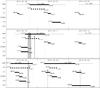 |
Fig. 1 Time diagram of the 2014 Feb.−Apr. campaign. The horizontal dashed lines are the XMM-Newton orbital visibility times of Sgr A* labeled with revolution numbers. The thick solid lines are the time slot of the observations for each instrument with start and stop hours. The vertical dotted lines are the limits of the XMM-Newton observations. The vertical gray blocks are the X-ray (Arabic numerals) and near-IR (Roman numerals) flares reported in this work. |
2.1. XMM-Newton observations
Table 1 reports the log of the
XMM-Newton campaign for 2014 Feb.−Apr. (AO-12; PI: N. Grosso). The last X-ray
observation is an anticipated Target of Opportunity (ToO) that was triggered to observe
the new flaring magnetar SGR J1745-29 (AO-12; PI: G.L.
Isra l). We only use the data from the EPIC
camera since the optical extinction towards the Galactic center is too high to get optical
or soft X-ray photons from Sgr A* with the Optical-UV Monitor or the Reflection Grating Spectrometers.
l). We only use the data from the EPIC
camera since the optical extinction towards the Galactic center is too high to get optical
or soft X-ray photons from Sgr A* with the Optical-UV Monitor or the Reflection Grating Spectrometers.
XMM-Newton observation log for the 2014 Feb.− Apr. campaign.
During the first three XMM-Newton observations, the two EPIC/MOS cameras (Turner et al. 2001) and the EPIC/pn camera (Strüder et al. 2001) observed in frame window mode. During the last observation, the two MOS cameras were in small window mode and the pn camera observed in frame window mode. All observations were made with the medium filter. The effective observation start and end times are reported in Table 1 in Universal Time (UT). During these observations, the conversion from the Terrestrial Time (TT) registered aboard XMM-Newton to UT is UT = TT−67.108s (NASA’s HEASARC Tool: xTime1). The total effective exposure for the four XMM-Newton observations during this campaign is ≈ 256 ks.
The XMM-Newton data reduction is the same as presented in Mossoux et al. (2015a). We used the Science Analysis Software (SAS) package (version 13.5) with the 2014 Apr. 4 release of the Current Calibration files (CCF) to reduce and analyze the data. The tasks emchain and epchain were used to create the event lists for the MOS and pn camera, respectively. The soft proton flare count rate in the full detector light curve in the 2−10 keV energy range was high (up to 0.02 count s-1 arcmin-2 in EPIC/pn) only during the last two hours of the third observation.
As we looked for variability of the X-ray emission from Sgr A*, we extracted events of the
source+background region from a disk of 10″-radius centered on the VLBI radio position of Sgr A*:  ,
,  (Reid et al. 1999). The contribution of the background events was estimated by
extracting a ≈ 3′ × 3′ region
at ≈ 4′ -north of Sgr
A* on the same CCD where the
X-ray emission is low. For the last observation, the background extraction region was a
≈ 3′ × 3′ area at
≈ 7′ -east of Sgr
A* on the adjacent CCD
because of the small window mode.
(Reid et al. 1999). The contribution of the background events was estimated by
extracting a ≈ 3′ × 3′ region
at ≈ 4′ -north of Sgr
A* on the same CCD where the
X-ray emission is low. For the last observation, the background extraction region was a
≈ 3′ × 3′ area at
≈ 7′ -east of Sgr
A* on the adjacent CCD
because of the small window mode.
The light curves of the source+background and background regions were created from events with PATTERN ≤ 12 and #XMMEA_SM and PATTERN ≤ 4 and FLAG==0 for the MOS and pn cameras, respectively. These light curves are computed in the 2−10 keV energy range using a time bin of 300 s. The task epiclccorr applies relative corrections to those light curves. We then summed the background-subtracted light curves of the three cameras to produce the total EPIC light curves. Missing values were inferred using a scaling factor between the pn camera and the sum of the MOS1 and MOS2 cameras. This factor was computed during the full time period where all detectors are observing and leads to a number of pn counts that is equal, on average, to 1.46 ± 0.03 times the sum of the number of MOS counts.
To perform the timing analysis of the light curves we adapted the Bayesian-blocks method developed by Scargle (1998) and refined by Scargle et al. (2013a) to the XMM-Newton event lists, using a two-step algorithm to correct for any detector flaring background (Mossoux et al. 2015a,b)2. We used the false detection probability p1 = exp(−3.5) (Neilsen et al. 2013; Mossoux et al. 2015a) and geometric priors of 7, 6.9, and 6.9 for pn, MOS1, and MOS2, respectively. We created smoothed light curves by applying a density estimator (Silverman 1986; Feigelson & Babu 2012) and using the same method as in Mossoux et al. (2015a) to correct the exposure time and the background contribution to the source+background event list. The amplitude and time of the flare maximum were computed on the smoothed light curve with a window width of 100 s and 500 s and a time grid interval of 10 s.
2.2. HST observations
The NIR observations of Sgr A* were obtained with the Wide Field Camera 3 (WFC3) on HST, under joint XMM-Newton/HST programs 13403 (AO-12, PI: N. Grosso) and 13316 (Cycle 21, PI: H. Bushouse) in order to measure the delay between X-ray flares and their NIR counterparts. Sgr A* was observed in four visits with 7−10 consecutive HST orbits, whose observation start and end times are reported in UT in Table 2. The total effective exposure for these four HST visits during the 2014 Feb.−Apr. campaign is about 69 ks. Exposures were taken constantly during each part of these windows in which Sgr A* was visible to HST, usually resulting in an uninterrupted cadence of exposures lasting for 40−50 min at a time, and then interrupted for the remaining 40−50 min of each HST orbit in which Sgr A* is occulted by the Earth. The four visits were planned to have the maximum number of consecutive orbits before HST entered the South Atlantic Anomaly (SAA), in order to maximize the simultaneous observing time in NIR and X-ray.
Observation log of WFC3 on board HST for the 2014 Feb.−Apr. campaign.
Each WFC3 exposure was taken with the IR channel of the camera, which has a
1024 × 1024 pixel HgCdTe
array, with a pixel scale of  . We used the F153M filter, which is a
medium-bandwidth filter (Δλ =
0.683 μm) with an effective wavelength λeff = 1.53157
μm (from the Spanish Virtual Observatory3). Each exposure used the predefined readout sequence
“SPARS25” with NSAMP = 12 or 13, which produces non-destructive readouts of the detector
every 25 secs throughout the exposure, and a total of 12 or 13 readouts, resulting in a
total exposure time of 275−300
s after discarding the first short (2.932 s) readout. The exposures were obtained in a 4-point dither
pattern centered on Sgr A*,
with a spacing of ~0.6
arcsec (~4 pixels) per
step to improve the sampling of the Point Spread Function (PSF) of
. We used the F153M filter, which is a
medium-bandwidth filter (Δλ =
0.683 μm) with an effective wavelength λeff = 1.53157
μm (from the Spanish Virtual Observatory3). Each exposure used the predefined readout sequence
“SPARS25” with NSAMP = 12 or 13, which produces non-destructive readouts of the detector
every 25 secs throughout the exposure, and a total of 12 or 13 readouts, resulting in a
total exposure time of 275−300
s after discarding the first short (2.932 s) readout. The exposures were obtained in a 4-point dither
pattern centered on Sgr A*,
with a spacing of ~0.6
arcsec (~4 pixels) per
step to improve the sampling of the Point Spread Function (PSF) of
 (1.136 detector pixels) at 1.50
μm (Dressel 2012)4.
All of the WFC3 exposures were calibrated using the standard STScI calibration pipeline
task calwf3. Once the pointing information was set for each WFC3
exposure, we could safely use the known relative position of Sgr A* for positioning a photometry aperture (Sgr
A* itself cannot be easily
identified in the WFC3 images because it is in the PSF wings of the star S2 located at
(1.136 detector pixels) at 1.50
μm (Dressel 2012)4.
All of the WFC3 exposures were calibrated using the standard STScI calibration pipeline
task calwf3. Once the pointing information was set for each WFC3
exposure, we could safely use the known relative position of Sgr A* for positioning a photometry aperture (Sgr
A* itself cannot be easily
identified in the WFC3 images because it is in the PSF wings of the star S2 located at
 during our observational epoch
according to the orbital elements of Gillessen et al.
2009).
during our observational epoch
according to the orbital elements of Gillessen et al.
2009).
The absolute coordinates of HST exposures are limited by uncertainties in the positions of the guide stars that are used to acquire and track the target. We therefore used the radio position of IRS-16C (also known as S96; Yusef-Zadeh et al. 2014), a star near Sgr A*, as an astrometric reference to accurately register the pointing of each WFC3 exposure. The radio position of IRS-16C came from VLA observations in February 2014, which is nearly co-eval with the HST observations.
The accumulating, non-destructive readouts of each calibrated exposure were “unraveled” by taking the difference of adjacent readouts, which results in a series of independent samples taken at 25 s intervals, thereby increasing the time resolution for the subsequent photometric analysis. Photometry of Sgr A* was performed with the IRAF routine phot, using a 3-pixel (~0.4 arcsec) diameter circular aperture centered on the known radio coordinates of Sgr A* (Petrov et al. 2011; Yusef-Zadeh et al. 2014).
Initial analysis of the photometry results for Sgr A* and other stars in the field revealed an overall tendency for the fluxes of individual sources to gradually decrease on the order of ~3% during the course of each individual exposure (i.e., across the span of multiple readouts). We believe this effect is due to persistence within an individual exposure, as the total signal level reaches fairly high levels by the end of each ~5 min exposure. We measured this trend for stars near Sgr A* and applied the results to the Sgr A* photometry to remove the effect. When applied to other stars in the field, the corrected photometry was constant, on average, throughout each exposure. The error on the photometry obtained in each of the four visits, within an individual 25 s readout interval, is 0.0044, 0.0046, 0.0022, and 0.0042 mJy, respectively, which has been estimated from the standard deviation of the flux density of a reference star. For comparison, similar observations obtained in the past using NICMOS camera 1 have an uncertainty within a bin of 32 s of 0.002 mJy at 1.60 μm (Yusef-Zadeh et al. 2006b).
Aperture and extinction corrections were also applied to the Sgr A* photometry. The aperture correction was determined by measuring the curves of growth of several isolated stars in the field, using a series of apertures of increasing size. The correction factor for an aperture diameter of 3 pixels is 1.414. The extinction correction was derived from A(H) = 4.35 ± 0.12 mag and A(Ks) = 2.46 ± 0.03 mag (Schödel et al. 2010) with λeff(NACO H) = 1.63725 μm and λeff(NACO Ks) = 2.12406 μm (from the Spanish Virtual Observatory), respectively, assuming a power law leading to A(λ) ∝ λ−2.19 ± 0.06. Thus, the computed extinction for the effective wavelength of the WFC3 F153M filter (λeff = 1.53157 μm) used is 5.03 ± 0.20 mag, which corresponds to a multiplicative factor of 103.2 ± 19.0 to correct the observed flux density for extinction.
2.3. VLT observations
Coordinated observation log with SINFONI at ESO’s VLT for the 2014 Feb.–Apr. campaign.
Near-infrared integral-field observations of the Galactic Center were performed using SINFONI at the VLT in Chile (Eisenhauer et al. 2003; Bonnet et al. 2004). Sgr A* was monitored nine times in 2014 Feb.−Apr.. Table 3 summarizes the observing log, including the amount of exposures that were selected for the analysis. The selection criteria is described below. These observations were planned to be coordinated with those carried out with XMM-Newton. Two of these observations were simultaneous with XMM-Newton observations and one was partially simultaneous. They are part of the ESO programs 092.B-0183(H) (PI: A. Eckart), 093.B-0932(A) (PI: N. Grosso), and 092.B-0920(A) (PI: N. Grosso) presented in Valencia-S. et al. (2015) for the DSO/G2 study.
The SINFONI instrument is an integral-field unit fed by an adaptive optics (AO) module.
The AO module was locked on a bright star 8 85
east and 1554
north of Sgr A*. The
H +
K grating used in these observations covers the
1.45 μm−2.45
μm range and exhibits a spectral resolution of
R ~
1500 (which corresponds to approximately 200 km s-1 at 2.16 μm). The smallest
SINFONI field of view (
85
east and 1554
north of Sgr A*. The
H +
K grating used in these observations covers the
1.45 μm−2.45
μm range and exhibits a spectral resolution of
R ~
1500 (which corresponds to approximately 200 km s-1 at 2.16 μm). The smallest
SINFONI field of view ( ) was jittered around the position of
S2. Observations of different B- and G-type stars were performed for further telluric
corrections.
) was jittered around the position of
S2. Observations of different B- and G-type stars were performed for further telluric
corrections.
Exposure times of 400 s were used to observe the Galactic center region, followed or preceded by observations on a dark cloud located about 12′45″ west and 5′36″ north of the Sgr A* sky position. These integration times were chosen to fully sample the variations of Sgr A* flux density over typical flare lengths, while optimizing the quality of the data.
The data processing and calibration was performed as described in Valencia-S. et al. (2015) and it is outlined here for completeness. First, bad lines were corrected using the procedure suggested in the SINFONI user manual. Then, a rough cosmic-ray correction in the sky and target exposures was performed using the algorithm of Pych (2004). Some science and calibration files showed random patterns that were detected and removed following the algorithms proposed by Smajić et al. (2014). Afterwards, the SINFONI pipeline was used for the standard reduction steps (e.g., flat fielding and bad pixel corrections) and for the wavelength calibration. A deep correction of cosmic rays and the atmospheric refraction effects were done using our own DPUSER routines (Thomas Ott, MPE Garching; see also Eckart & Duhoux 1991).
The quality of individual exposures was judged based on the point-spread function (PSF) at the moment of the observation. The PSF was estimated by fitting a 2D Gaussian to the bright star S2. Data cubes where the full width at half maximum of the Gaussian was higher than 96 mas (or 7.65 detector pixels) were discarded in the analysis. The 2014 Feb. 28, Mar. 1, and Mar. 2 observations are thus not used because of their poor quality. On 2014 Apr. 2 two data cubes of larger field-of-view were used for pointing. They were not included in the light curves since they map regions just beside the central S-cluster. Flux calibration on individual data cubes was performed using aperture photometry on the deconvolved K-band image. The deconvolution was done using the Lucy–Richardson algorithm in DPUSER. For calibration we used the stars S2 (Ks = 14.13), S4 (Ks = 14.61), S10 (Ks = 14.12), and S12 (Ks = 15.49), and adopted the Ks-band extinction correction A(Ks) = 2.46 ± 0.03 mag (Schödel et al. 2010). Additional information on the flux estimation is given by Witzel et al. (2012). The final flux densities were extracted by fitting a 2D Gaussian to the calibrated continuum images for all time steps.
2.4. VLA observations
VLA observation log for the 2014 Feb.−Apr. campaign.
Radio continuum observations were carried out with the Karl G. Jansky Very Large Array (VLA) on 2014 March 1, March 10 and April 2 (observing program 14A-231). The VLA was in its A-configuration during these three days of observations, with start and stop times reported in Table 4. In all observations, we used 3C 286 to calibrate the flux density scale, both 3C286 and NRAO530 to calibrate the bandpass, and J1744-3116 to calibrate the complex gains.
On 2014 Mar. 1 we observed Sgr A* at 8−10 GHz (X-Band) using the 8-bit sampler system with 2 GHz total bandwidth, each consisting of 64 channels each 2 MHz wide. On 2014 Mar. 10 we used the same correlator setup as 2014 Mar. 1, except using the Ku-Band between 13 and 15 GHz. On 2014 Apr. 2 we used the two bands 5−7 GHz (C-band) and 1−2 GHz (L-band), and alternated between these bands every 7 minutes. The C-band correlator was set-up similarly to that of X-band. The L-band correlator, however, used 1 GHz of bandwidth, which consisted of 16 IFs with channel widths of 1 MHz each. After primary calibration using OBIT (Cotton 2008), a self-calibration procedure was applied using AIPS in phase only, to remove atmospheric phase errors.
2.5. CARMA observations
CARMA 95 GHz observation log for the 2014 Feb.− Apr. campaign.
Observations of Sgr A* at 95 GHz (corresponding to 3.2 mm) were obtained with CARMA on 2014 Mar. 10, Apr. 2, and Apr. 3 (see Table 5). The array was in the C-configuration, with antenna separations ranging from 30–350 meters. The correlator processed frequencies range was 88.76−93.24 GHz in the lower sideband of the receivers and 96.76−101.24 GHz in the upper sideband. The spectral resolution was 25 MHz after Hanning smoothing. Channels corresponding to strong absorption lines of HCO+ (89.19 GHz), HNC (90.65 GHz), and CS (97.98 GHz) were dropped from Sgr A* data before averaging to get the continuum flux density. Only visibility data corresponding to telescope separations larger than 20 kλ were used for the flux measurements, to reduce contamination from extended emission near Sgr A*.
Observations of 3C279 were used to calibrate the instrumental passband. The flux density
scale was established from observations of Neptune, assuming it is a
22
diameter disk with brightness temperature 123 K (consistent with the Butler-JPL-Horizons
2012 model shown in ALMA memo 594). Observations of a secondary flux calibrator (the
blazar 1733−130, a.k.a. NRAO
530) were interleaved with the Sgr A* observations every 15 minutes to monitor the antenna gains. The flux
density of 1733−130 was
measured to be 2.7 ± 0.3 Jy on
2014 Mar. 10, and 2.5 ± 0.3 Jy
on Apr. 2 and Apr. 3, relative to Neptune.
The data on Mar. 10 were obtained in turbulent weather and are of poor quality, therefore we do not use it in this work. On 2014 Apr. 2 we only use the data before the beginning of the snow at about 12:30 UT.
3. Data analysis
3.1. XMM-Newton data
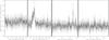 |
Fig. 2 XMM-Newton/EPIC (pn+MOS1+MOS2) light curves of Sgr A* in the 2−10 keV energy range obtained 2014 Feb.−Apr. The time interval used to bin the light curve is 300 s. The X-ray flares are labeled with Arabic numerals. The horizontal lines below these labels indicate the flare durations. |
Figure 2 shows the XMM-Newton/EPIC
(pn+MOS1+MOS2) background-subtracted light curves of Sgr A* binned to 300 s in the 2−10 keV energy range. The non-flaring level
(i.e., the longest interval of the Bayesian blocks) during 2014 Feb.−Apr. is about 3 times the typical value of
0.18 count s-1
(e.g., Porquet et al. 2008; Mossoux et al. 2015a). This is due to the flaring magnetar SGR J1745-29
located only 24
from Sgr A* (Rea et al. 2013). Because the radius enclosing 50% of
the energy for EPIC/pn at 1.5 keV on-axis is about 10″ (Ghizzardi
2002), we extract the events from a 10″-radius circle centered on Sgr A* as done in previous studies. This
extraction region therefore includes events from SGR J1745-29, which artificially
increases the non-flaring level of Sgr A* (Fig. 2).
3.1.1. Impact of the magnetar on the flare detection
Degenaar et al. (2013) reported a large flare
towards Sgr A* detected by
Swift on 2013 Apr. 24. The detection of a hard X-ray burst by BAT near Sgr
A* on 2013 Apr. 25 led
Kennea et al. (2013) to attribute this flux
increase to a new Soft Gamma Repeater unresolved from Sgr A*: SGR J1745-29. The X-ray spectrum of
this magnetar is an absorbed blackbody with 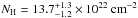 and kTBB = 1.06 ±
0.06 keV (Kennea et al. 2013).
But the Chandra X-ray Observatory (CXO) results between 1 and 10 keV
from Coti Zelati et al. (2015) show that the
temperature of the blackbody emitting region decreases with time: kTBB/ keV =
(0.85 ± 0.01)−(1.77 ± 0.04) × 10-4(t −
t0) with t0 the time of
the peak outburst (i.e., 2013 Apr. 24 or 56 406 in MJD). They show that before 100 d
from outburst, the magnetar luminosity between 1 and 10 keV is characterized by a linear
model plus an exponential decay whose e-folding time is 37 ± 2 d. After 100 d from the burst
activation, the magnetar flux is well fitted by an exponential with an e-folding time of
253 ± 5 d. This flux decay
is one of the slower decays observed for a magnetar. Thanks to 8 months of observations
with the Green Bank Telescope and 18 months of observations with the Swift’s X-Ray
Telescope, the evolution of the X-ray flux and spin period of the magnetar have been
well constrained by Lynch et al. (2015). The
X-ray flux between 2 and 10 keV in a 20″-radius extraction region centered on the magnetar decreases as
the sum of two exponentials: F(t) = (1.00 ± 0.06) e−(t −
t0)/(55 ± 7 d) + (0.98 ± 0.07)
e−(t − t0)/(500 ± 41
d) in unit of 10-11 erg s-1 cm-2 with
t0 the same as in Coti Zelati et al. (2015).
and kTBB = 1.06 ±
0.06 keV (Kennea et al. 2013).
But the Chandra X-ray Observatory (CXO) results between 1 and 10 keV
from Coti Zelati et al. (2015) show that the
temperature of the blackbody emitting region decreases with time: kTBB/ keV =
(0.85 ± 0.01)−(1.77 ± 0.04) × 10-4(t −
t0) with t0 the time of
the peak outburst (i.e., 2013 Apr. 24 or 56 406 in MJD). They show that before 100 d
from outburst, the magnetar luminosity between 1 and 10 keV is characterized by a linear
model plus an exponential decay whose e-folding time is 37 ± 2 d. After 100 d from the burst
activation, the magnetar flux is well fitted by an exponential with an e-folding time of
253 ± 5 d. This flux decay
is one of the slower decays observed for a magnetar. Thanks to 8 months of observations
with the Green Bank Telescope and 18 months of observations with the Swift’s X-Ray
Telescope, the evolution of the X-ray flux and spin period of the magnetar have been
well constrained by Lynch et al. (2015). The
X-ray flux between 2 and 10 keV in a 20″-radius extraction region centered on the magnetar decreases as
the sum of two exponentials: F(t) = (1.00 ± 0.06) e−(t −
t0)/(55 ± 7 d) + (0.98 ± 0.07)
e−(t − t0)/(500 ± 41
d) in unit of 10-11 erg s-1 cm-2 with
t0 the same as in Coti Zelati et al. (2015).
We determined the exponential decay of the magnetar flux between 2 and 10 keV by applying a chi-squared fitting of the non-flaring level of each observation computed using the Bayesian-blocks algorithm: on Feb. 28, Mar. 10, and Apr. 2 and 3 the non-flaring level is 0.562 ± 0.003, 0.528 ± 0.004, 0.489 ± 0.003 and 0.499 ± 0.002 EPIC count s-1, respectively. The magnetar flux variation can be described as N(t) = N0 e−(t − t0) /τ with t the time corresponding to the middle of each observation, t0 and N0 the time and count rate of the non-flaring level of the first observation, and τ the decay time scale. Our best fit parameters with corresponding 1σ uncertainties are: N0 = 0.558 ± 0.003 count s-1 and τ = 281 ± 15 days. The decay time scale is about 2 times shorter than those computed from the formula of Lynch et al. (2015) for this date. However, as we can see in Fig. 2 of Lynch et al. (2015), the magnetar flux is not a perfect exponential decay and has some local increase of the flux, in particular during our observing period. This is seen in the last XMM-Newton/EPIC pn observation on 2014 Apr. 3, which is characterized by two blocks whose change point is at 16:27:48 (UTC). The corresponding count rates for the first and second blocks are 0.254 ± 0.03 and 0.299 ± 0.03 pn count s-1. By folding light curves for each block on this date with the magnetar spin period of 3.76398106 s computed in Appendix B, we see that the pulse shape has not changed, but the flux increased by a factor of about 1.2, as determined by the Bayesian-blocks algorithm. Moreover, the Chandra monitoring of DSO/G2 shows that there is no significant increase of Sgr A* flux on 2014 Apr. 4 (Haggard et al. 2014).
This contamination of the non-flaring level implies a decrease of the detection level of the faintest and shortest flares, as explained in details in Appendix A. Comparing the detection probability of an XMM-Newton observation with the distribution of flares during the 2012 Chandra XVP campaign (Neilsen et al. 2013), we estimate that we lost no more than one flare during our four XMM-Newton observations due to the magnetar contribution.
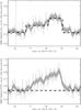 |
Fig. 3 XMM-Newton light curve binned on 500 s of the 2014 Mar. 10 flare from Sgr A* in the 2−10 keV energy range. Top panel: the crosses are the data points of the EPIC/pn light curve. The dashed lines represent the Bayesian blocks. The solid line and the gray curve are the smoothed light curve and the associated errors (h = 500 s). Bottom panel: the total (pn+MOS1+MOS2) light curve. The horizontal dashed line and the solid line are the sum of the non-flaring level and the smoothed light curve for each instrument. The vertical gray stripe is the time during which the camera did not observe. |
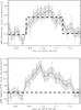 |
Fig. 4 XMM-Newton light curve binned on 100 s of the 2014 Apr. 2 flare from Sgr A* in the 2−10 keV energy range. The window width of the smoothed light curve is 100 s. See caption of Fig. 3 for panel description. |
3.1.2. X-ray flare detection
By applying the Bayesian-blocks analysis on the EPIC event lists, we are able to detect two flares: one on 2014 Mar. 10 and one on 2014 Apr. 2. These flares are labeled 1 to 2 in Fig. 2. Figures 3 and 4 focus on the EPIC (pn+MOS1+MOS2) and EPIC/pn flare light curves with a bin time interval of 500 and 100 s, respectively. The comparison of the flare light curves observed by each EPIC cameras can be found in Appendix C. The second flare is detected by the Bayesian-blocks algorithm in pn, but not in MOS1 or MOS2. This is explained by the lower sensitivity of the MOS cameras, resulting in a lower detection level of the algorithm (see Fig. A.1). Table 6 gives the temporal characteristics of these X-ray flares.
Characteristics of the X-ray flares observed by XMM-Newton in 2014 after removing the magnetar contribution.
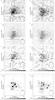 |
Fig. 5 XMM-Newton/MOS1 (left column) and MOS2
(right column) images of Sgr A* on 2014 Mar. 10. The energy range
is 2–10 keV. The field of view is 20″ ×
20″, the pixel size is |

We removed the magnetar contribution from the Sgr A* EPIC/pn event list in order to increase the detection level of the flares. This was done by computing the period and period derivative of SGR J1745-29 and filtering out time intervals where the magnetar flux is less than 50% of its total flux (see Appendix B for details). We only work with EPIC/pn, because it has a better temporal resolution (73.4 ms) than the EPIC/MOS cameras (2.6 s; ESA: XMM-Newton SOC 2013). By applying the Bayesian-blocks analysis on the filtered pn event lists, we find no additional flares, and the start and end times of the already detected flares do not change significantly.
The flare detected on 2014 Mar. 10 is characterized by a long rise (~7700 s) and a rapid decay (~844 s). This is one of the longest flares ever observed in X-ray, with a duration of about 8.5 ks. For comparison, the largest flare observed during the Chandra XVP 2012 campaign has a duration of 7.9 ks and the first flare detected from Sgr A* observed by Baganoff et al. (2001) had a duration of ~10 ks. In EPIC/pn, the Bayesian-blocks algorithm divides the flare into two blocks, but in EPIC/MOS1 and MOS2 this flare is described with only one Bayesian block.
To localize the origin of this flaring emission we focus on the MOS observations, which
provide a good sampling of the X-ray PSF ( ) thanks to their
 pixels. We first compute sky images
that match the detector sampling for the flaring and non-flaring periods, and then we
look for any significant excess counts during the flaring period compared to the
non-flaring one, using the Bayesian method of Kraft et
al. (1991).
pixels. We first compute sky images
that match the detector sampling for the flaring and non-flaring periods, and then we
look for any significant excess counts during the flaring period compared to the
non-flaring one, using the Bayesian method of Kraft et
al. (1991).
We have suppressed the randomization of the event position inside the detector pixel
during the production of the event list, therefore the event is assigned to the center
of the detector pixel and its sky coordinates are reconstructed from the spacecraft
attitude with an angular resolution of  . We filter the X-ray events using
the (softer) #XMMEA_EM flag (e.g., bad rows are filtered out,
keeping adjacent rows) and we select only events with the best positioning (single-pixel
events, corresponding to pattern=0) and 2–10 keV energy. We first
assess the mean sky position of the detector pixel that was the closest to Sgr
A* by comparing the event
sky positions with the pattern of the spacecraft offsets from the mean pointing that we
derived from the attitude history file (*SC*ATS.FIT). We then
compute images and exposure maps centered on this sky position with
sky-pixels for the flaring and
non-flaring periods (see Appendix C for the
definition of the Bayesian blocks). There is no moiré effect in these images, because
the mean position-angle of the detector (90.̊78) is very close to 90°. Panels a and b of Fig. 5 show the MOS1 and MOS2 count numbers during the
flaring period. Following Kraft et al. (1991) we
denote this image N. The horizontal row with no counts in the MOS1
image is due to a bad row. Panels c and d of Fig. 5
show the MOS1 and MOS2 count numbers during the non-flaring period, scaled-down to the
flaring-period exposure using the exposure map ratios. This image is our estimate of the
mean count numbers during the non-flaring period. Following Kraft et al. (1991) we denote this image B, as background. Panels
e and f of Fig. 5 show the difference between the
previous panels, shown only for potential count excesses (N − B>
0). Following Kraft et al.
(1991) we denote this image S, as source. Poisson statistics are required due
to the low number of counts, hence we have to carefully determine the confidence limits
of the observed count excesses to select only pixels that exclude null values at the
confidence level CL.
. We filter the X-ray events using
the (softer) #XMMEA_EM flag (e.g., bad rows are filtered out,
keeping adjacent rows) and we select only events with the best positioning (single-pixel
events, corresponding to pattern=0) and 2–10 keV energy. We first
assess the mean sky position of the detector pixel that was the closest to Sgr
A* by comparing the event
sky positions with the pattern of the spacecraft offsets from the mean pointing that we
derived from the attitude history file (*SC*ATS.FIT). We then
compute images and exposure maps centered on this sky position with
sky-pixels for the flaring and
non-flaring periods (see Appendix C for the
definition of the Bayesian blocks). There is no moiré effect in these images, because
the mean position-angle of the detector (90.̊78) is very close to 90°. Panels a and b of Fig. 5 show the MOS1 and MOS2 count numbers during the
flaring period. Following Kraft et al. (1991) we
denote this image N. The horizontal row with no counts in the MOS1
image is due to a bad row. Panels c and d of Fig. 5
show the MOS1 and MOS2 count numbers during the non-flaring period, scaled-down to the
flaring-period exposure using the exposure map ratios. This image is our estimate of the
mean count numbers during the non-flaring period. Following Kraft et al. (1991) we denote this image B, as background. Panels
e and f of Fig. 5 show the difference between the
previous panels, shown only for potential count excesses (N − B>
0). Following Kraft et al.
(1991) we denote this image S, as source. Poisson statistics are required due
to the low number of counts, hence we have to carefully determine the confidence limits
of the observed count excesses to select only pixels that exclude null values at the
confidence level CL.
Since the Bayesian method of Kraft et al. (1991) requires that the background estimate is close to the true value (see also Helene 1983), we limit our statistical analysis to the pixels where the count number during the non-flaring period is larger or equal to 20, in order to reduce the Poisson noise (see the boxed pixel areas in panels g and h of Fig. 5). We compute the confidence level for each count excess using Eq. (9) of Kraft et al. (1991)5 and convert it to a Gaussian equivalent in units of σ. Panels g and h of Fig. 5 show pixels with confidence levels that are larger or equal to 3σ. The barycenters of these pixels weighted by their count excesses (diamonds in panels g and h of Fig. 5) are consistent with the position of Sgr A* when considering the absolute astrometry uncertainty of EPIC, which confirms that the flaring emission detected on 2014 Mar. 10 came from Sgr A*.
3.1.3. Spectral analysis of the X-ray flares
Spectral properties of the X-ray flares observed by XMM-Newton.
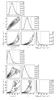 |
Fig. 6 Best-fit parameters of the 2014 Mar. 10 (top) and 2014 Apr. 2 (bottom) flares. The diagonal plots are the marginal density distribution of each parameter. The median values of each parameter are represented by the vertical dotted lines in diagonal plots and by a cross in other panels; the vertical dashed lines define the 90% confidence interval (see Table 7 for the exact values). The contours are 68%, 90% and 99% of confidence levels. |
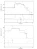 |
Fig. 7 XMM-Newton/EPIC pn spectrum of the 2014 Mar. 10 (top) and 2014 Apr 2 (bottom) flares. The model is the best spectrum obtained with MCMC (see text for details). The lower panel in the two graphs is the residual. The horizontal and vertical lines are the spectral bins and the error on the data, respectively. |
To analyze the spectrum of the two flares seen by XMM-Newton on 2014 Mar. 10 and 2014 Apr. 2, we extracted events from a circle of 10″ radius centered on the Sgr A* radio position, as we did for the temporal analysis. The X-ray photons were selected with PATTERN≤ 4 and FLAG==0 for the pn camera. We did not work with photons from MOS1 and MOS2, because the number of events is too small to constrain the spectral properties. The source+background time interval is the range between the beginning and the end of the flare computed by the Bayesian-blocks algorithm (see Table 6). The background time interval is the whole observation minus the time range during the flare. We also rejected 300 s on either side of the flare to avoid any bias. This extraction is the same as used in Mossoux et al. (2015a). We computed the spectrum, ancillary files, and response matrices with the SAS task especget.
The model used to fit the spectrum with XSPEC (version 12.8.1o) is the same as that in Mossoux et al. (2015a): an absorbed power law created using TBnew (Wilms et al. 2000) and pegpwrlw with a dust scattering model from dustscat (Predehl & Schmitt 1995). TBnew uses the cross-sections from Verner et al. (1996). Interstellar medium abundances of Wilms et al. (2000) imply a decrease of the column density by a factor of 1.5 (Nowak et al. 2012). The extracted spectrum was grouped using the SAS task specgroup. The spectral binning begins at 2 keV with a minimum signal-to-noise ratio6 of 4 and 3 for the first and second flares, respectively. The number of net counts during the first flare is 900 (see Table 6) and the number of spectral bins is 12. This gives an average of about 75 counts in each spectral bin. If we perform the same computation for the second flare, which has 180 net counts for 6 spectral bins, we have 31 counts per spectral bin.
We used the Markov Chain Monte Carlo (MCMC) algorithm to constrain the three parameters
of the model: the hydrogen column density (NH), the photon index of the power law
(Γ), and the unabsorbed
flux between 2 and 10 keV ( ). The MCMC makes a random walk of
nstep
steps in parameter space for several walkers (nwalkers), which evolve simultaneously. The
position of each walker at a step in the parameter space is determined by the positions
of the walker at the previous step. Convergence was achieved using the probability
function of the parameters. The resulting MCMC chain reports all these steps. This
method give us a complete view of the spectral parameters distribution and correlation.
). The MCMC makes a random walk of
nstep
steps in parameter space for several walkers (nwalkers), which evolve simultaneously. The
position of each walker at a step in the parameter space is determined by the positions
of the walker at the previous step. Convergence was achieved using the probability
function of the parameters. The resulting MCMC chain reports all these steps. This
method give us a complete view of the spectral parameters distribution and correlation.
We use Jeremy Sanders’ XSPEC_emcee7 program that allows MCMC analyses of X-ray spectra in XSPEC using emcee8 (Foreman-Mackey et al. 2013), an extensible, pure Python implementation of Goodman & Weare (2010)’s affine invariant MCMC ensemble sampler. We follow the operating mode explained in the XSPEC_emcee homepage to find the optimal value for the MCMC sampler parameters. Two criteria must be fulfilled to have a good sampling in the chain: the chain length must be greater than the autocorrelation time and the mean acceptance fraction must be between 0.2 and 0.5 (Foreman-Mackey et al. 2013). We created a chain containing 30 walkers. The Python function acor computes the auto-correlation time (τacor) needed to have an independent sampling of the target density. The burn-in period (nburn) and chain length (nstep) are defined as 20 × τacor (Sokal 1997) and 30 × nburn (Foreman-Mackey et al. 2013), respectively. For the spectral model used here, τacor = 5.1 and 5.3 for the 2014 Mar. 10 and 2014 Apr. 2 flares, respectively. Thus we used nburn = 102, nwalkers = 30, and nstep = 3060 for the March 10 flare and nburn = 106, nwalkers = 30, and nstep = 3180 for the April 2 flare. The mean acceptance fraction is around 0.6 for the two flares, which is a reliable value.
The diagonal plots in Fig. 6 are the marginal distribution of each parameter (i.e., the probability to have a certain value of one parameter independently from others). The other panels in Fig. 6 represent the joint probability for each pair of parameters. The contours indicate the parameter region where there are 68%, 90% and 99% of the points (i.e., nwalkers × nstep). The best-fit parameter values are the median (i.e., 50th percentile) of each parameter obtained from the marginal distribution. We also define a 90% confidence range for each parameter as the 5th and 95th percentile of the marginal distribution. These numbers are reported in Table 7. The corresponding best spectrum is over-plotted on the data in Fig. 7.
We can compare the spectral parameters of this flare with those of the two brightest flares detected with XMM-Newton, which have the better constrained spectral parameters thanks to the high throughput and no pileup (Porquet et al. 2003, 2008). Their spectral properties are reported in Table 7. The magnetar has a soft spectrum, which implies that the soft part (0.5−3 keV) of the background is very high. Thus we have only one spectral bin in this energy band (see Fig. 7), implying that the hydrogen column density is not well constrained. The hydrogen column density and the photon index of the two brightest flares are well within the 90% confidence range of the 2014 Mar. 10 and 2014 Apr. 2 flares even if the parameters of the latter are less constrained than the former.
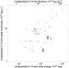 |
Fig. 8 Unabsorbed total energy vs. unabsorbed peak luminosity of the X-ray flares (adapted from Mossoux et al. 2015a). The top x-axis is the unabsorbed fluence. The crosses represent the X-ray flares from the Chandra XVP campaign (Neilsen et al. 2013), the triangles are the two brightest flares seen with XMM-Newton (Porquet et al. 2003, 2008), the diamond and the two squares are the 2011 March 30 flare and its subflares, respectively (Mossoux et al. 2015a). The empty circles are X-ray flares 1 and 2 of this work with their 1σ error bars. The filled circles are the components 1a and 1b of flare 1 (see Sect. 4.1.2). |
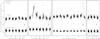 |
Fig. 9 Light curves of Sgr A* obtained with WFC3 on board HST during 2014 Feb.−Apr. The NIR flares are labeled with Roman numerals. The horizontal lines below these labels indicate the flare durations. The error bar in each panel is standard deviation of the photometry. |
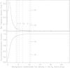 |
Fig. 10 Histogram of the NIR flux densities from Sgr A* observed in the Ks-band with NACO at ESO’s VLT (adapted from Fig. 3 of Witzel et al. 2012). Top panel: the solid line is the normalized distribution of the NIR flux densities corrected from the background emission. The dashed lines are the amplitude of the HST flares I, II and the lower limit of the amplitude of the flare III extrapolated to the Ks-band. We also represented the amplitude above the 3σ limit of the VLT flares IV and V extrapolated to the Ks-band. The dot-dashed line is the detection limit corresponding to 3 times the standard deviation of the quiescent flux density of HST on 2014 Mar. 10. Bottom panel: the cumulative distribution function of the NIR flux densities from Sgr A* corrected from the background emission. |
Assuming the typical spectral parameters of the X-ray bright flares, i.e., Γ = 2 and NH = 14.3 × 1022 cm-2 (Porquet et al. 2003, 2008; Nowak et al. 2012), we determined with XSPEC and the pn response files in the 2−10 keV energy range an unabsorbed-flux-to-count-rate ratio of 4.41 × 10⁻¹¹ erg s-1 cm-2/ pn count s-1 (corresponding to an absorbed-flux-to-count-rate ratio of 2.01 × 10⁻¹¹ erg s-1 cm-2/ pn count s-1). From the 8 kpc distance and the total number of counts (Table 6), we determine a total energy of 30.4 ± 1.9 × 1037 and 6.0 ± 0.4 × 1037 ergs (1σ error) for the 2014 Mar. 10 and Apr. 2 flares, respectively. These values can be compared to flares previously observed with Chandra and XMM-Newton. Figure 8 shows the total energy of these flares versus the unabsorbed peak luminosity. Flare 1 is one of the most energetic flares, due to its very long duration. The peak amplitude and total energy of flare 2 is close to the median values observed for this flare sample.
3.2. HST data
The HST light curves of Sgr A* and a reference star for the four visits are shown in Fig. 9. The error bar in each panel represents the typical uncertainty on the photometry derived for the reference star (standard deviation of the photometry). The deredened non-flaring flux density of Sgr A* and the corresponding error, computed using a 1σ-clipping method, are 59.3 ± 0.7, 60.1 ± 0.9, 60.8 ± 1.1 and 60.3 ± 0.8 mJy on 2014 Feb. 28, Mar. 10, Apr. 2, and Apr. 3, respectively (horizontal dot-dashed line of Fig. 9). The beginning and end of each flare is set by the 1σ limit on the flux density whose maximum amplitude is larger than 3σ. We only considered flux-density increases that lasted longer than 25 s, in order to discard any calibration glitchs. All observed NIR flares are labeled with Roman numerals.
The ~10 h visit on 2014 Mar. 10 detected two NIR flares. The first one (labeled I) peaks at 8.2σ and has an X-ray counterpart. It lasts from 16:29:51 to 18:52:36 (1σ limit). We can see in Table 6 that it begins and ends ~14 min before the X-ray flare. As for the X-ray flare, its shape is not a Gaussian, as it has a dip during the third HST orbit. Two interpretations can be made to explain this shape. First, this flare could be a single flare and the variation from Gaussian shape during the third orbit can be seen as substructures, as is the case for some NIR flares (Dodds-Eden et al. 2009). The second interpretation is that this NIR flare is in fact two distinct flares with a return below the 1σ limit between ~18:30 and ~18:39. The time delay between the two maxima in this scenario would be about 90 min. From 21:32:33 to 22:02:58 on 2014 Mar. 10, we can see that there is a second NIR flare (labeled II), which has no X-ray counterpart. Its maximum is about 3.4σ.
On 2014 Apr. 2 we caught the end of a NIR flare (labeled III), lasting until 17:31:15. Its amplitude is larger than 8.8σ, since its maximum occured during the Earth occultation of Sgr A*. Its beginning could correspond with the small increase in flux density seen just before the start of the Earth occultation of Sgr A*, which would lead to an upper limit on its duration of 3360 s. The duration of this NIR flare III and its possible relation with X-ray flare 2 will be discussed in Sect. 4.
The amplitudes of these flares can be compared to the sample of flux densities from Sgr A* observed in the Ks-band with NACO at ESO’s VLT and reported by Witzel et al. (2012). They constructed a histogram of all flux densities from the light curves, without distinction between the quiescent and flaring periods. This observed distribution of the flux density has a relative maximum at 3.57 mJy. Below this amplitude the distribution decreases, because of the detection limit of NACO. Above 3.57 mJy, the distribution is highly asymmetric, with a rapid decay of the frequency density followed by a long tail to 32 mJy. Figure 10 compares the amplitude of the flares detected with HST during this campaign with the relative frequency density given in Witzel et al. (2012, Fig. 3). The normalized distribution of the NIR flux densities observed with NACO (top panel of Fig. 10) is corrected for the background emission of 0.6 mJy (Witzel et al. 2012). The amplitude of the flares detected with HST are extrapolated to the Ks-band using the H − L spectral index of Sgr A* computed in Witzel et al. (2014b), which is α = −0.62.
The detection threshold of HST, which we define as the 3σ limit (dot-dashed line in Fig. 10), corresponds to 8% of the amplitude sample observed with NACO (bottom panel of Fig. 10). The amplitude of NIR flare II is about 7 times smaller than the amplitude of the brightest flare observed with NACO, whereas the amplitude of flare I is only 3 times smaller than the amplitude of this event. We can only measure a lower limit on the amplitude of NIR flare III, since its maximum occured during the Earth occultation. This lower limit is nearly as large as those of flare I.
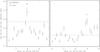 |
Fig. 11 Light curves of Sgr A* obtained with SINFONI at ESO’s VLT during 2014 Apr. 3 and 4. The dash-dotted lines represent the 3σ detection level of Sgr A*. The horizontal segments indicate the exposure length of 400 s. The NIR flares are labeled with Roman numerals. |
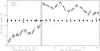 |
Fig. 12 CARMA light curves at 3.2 mm (95 GHz) of Sgr A* (white circle) and 1733-130 (black circle) in April 2014. The dash-dotted line represents the mean flux density. |
3.3. VLT data
Figure 11 shows the ratio between Sgr A* and S2 flux densities for the observations where a NIR flare was detected. Making a very conservative estimation, the 3σ detection levels of Sgr A* in the 2014 Apr. 3 and 4 data yield flux density ratios of F(Sgr A∗) /F(S2) ≈ 0.37 and 0.22, respectively (dash-dotted lines of Fig. 11). A flare (labeled IV) is observed on 2014 Apr. 3 with a peak amplitude of ~3.9σ. We clearly see its rise and decay phase below the 3σ detection level. On 2014 Apr. 4, a smaller flare (labeled V) is seen around 9:00 UT with a peak amplitude of ~5.1σ.
Using Eq. (2) of Witzel et al. (2012), with Ks(S2) = 14.13 ± 0.01 and A(Ks) = 2.46 ± 0.03 (Schödel et al. 2010), we have F(S2) = 14.32 ± 0.26 mJy. The amplitude of the two NIR flares detected with SINFONI are thus 6.92 ± 0.13 and 5.30 ± 0.09 mJy for 2014 Apr. 3 and 4, respectively. We consider that all the SINFONI light curve variations above our 3σ detection limit can be attributed to Sgr A* activity. We can therefore compare these flux densities with the sample of flux densities observed with NACO after the background subtraction of 0.6 mJy (Fig. 10). The 2014 Apr. 3 and 4 flares are within 4% of the largest amplitude, and are 5 and 6 times smaller than the brightest amplitudes observed with NACO, respectively. The 3σ detection level corresponds to 3.15 ± 0.06 mJy, which is comparable to the 11% of the largest flux density observed with NACO (Fig. 10).
3.4. CARMA data
The flux densities at 95 GHz (3.2 mm) of Sgr A* and 1733−130 shown in Fig. 12 are computed for each 10 s integration on 2014 Apr. 2 and 3. On 2014 Apr. 2 the flux density of Sgr A* increases slowly. A bump is seen at 11.3 h, but it could not be associated with the observed NIR or X-ray flares, since the CARMA observation occurred before the flares observed with HST and XMM-Newton.
On 2014 Apr. 3 the flux density decreases slowly, with two bumps occuring at 12.4 and 13.6 h. The maximum of the NIR flare IV observed with VLT occurred at 7.9 h on the same date. One of these episodes of radio flux density variation could be the delayed emission from this NIR flare, which would indicate a time delay of 4.4 or 5.6 h for the first and second bumps, respectively. The delays previously measured between the X-rays and the 850 μm light curves range between 1.3 and 2.7 h (e.g., Yusef-Zadeh et al. 2006b, 2008; Marrone et al. 2008). Assuming the expanding plasmon model, the delay between the NIR and the longer wavelength (3.2 mm) emission must be larger than these values, leading to a time delay consistent with those measured for these two bumps. One time-delay measurement was made between the X-rays and the 7 mm light curve, leading to a delay of about 5.3 h (Yusef-Zadeh et al. 2009). This measure seems to reject the second bump as being the delayed sub-mm emission from the VLT flare, since the delay is too long. The first bump, therefore, could be the delayed millimeter emission of the NIR flare IV. The second bump could then be the delayed millimeter emission of a NIR flare whose peak is lower than the 3σ detection level of VLT or which occurred after the end of the VLT observation and during Earth occultation for HST.
The flux density of Sgr A* during these observations increases with frequency as Sν ∝ ν0.2. For comparison, previous observations of Sgr A* between 43.3, 95.0, and 151 GHz (corresponding to 7.0, 3.2, and 2.0 mm; Table 2 of Falcke et al. 1998) give a similar spectra index of 0.58 ± 0.23.
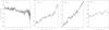 |
Fig. 13 VLA light curves of Sgr A* obtained on 2014 Mar. 1 (8.56 GHz), Mar. 10 (13.37 GHz) and Apr. 2 (1.68 and 5.19 GHz). The y-axis covers the same range of flux density for all observation and is centered on the mean of the minimum and maximum flux density in each panel. |
3.5. VLA data
We obtained light curves of Sgr A* from all three days of VLA observations, selecting (for the purpose of simplification) only one intermediate frequency channel with 30 s of averaging (analysis of the full radio dataset will be given elsewhere). In all observations we selected visibilities greater than 100 kλ in order to minimize contamination from extended thermal emission from Sgr A West. The radio light curves for the frequencies obtained with the VLA in configuration A on 2014 Mar.−Apr. are shown in Fig. 13.
We interleaved the CARMA and VLA L- and C-band observations from 2014 Apr. 2 in order to search for a time delay between the 1.68 GHz and 5.14 GHz, and the 1.68 GHz and 95 GHz light curves, using the z-transformed discrete correlation function (ZDCF; Alexander 1997). The cross-correlation graphs show no significant maximum of the likelihood function, implying that we can not derive any time delay between these light curves.
The light curves on 2014 Mar. 1 and Apr. 2 display a steady decrease and increase of flux
density. The light curve on 2014 Mar. 10 shows an obvious break in its rising flux density
around 16 h, with a clear increase of the rising slope. To better constrain the time of
this slope change, we fit the VLA light curve with a broken line. The break is located at
15.7 ± 0.2 h with a slope
increasing from 9.7 ± 0.1 to
27 ± 1 mJy h-1
( with 508 d.o.f.), which is significant. We
therefore tentatively attribute it to the onset of a radio flare, since we have only
partial temporal coverage of this radio event. For comparison purposes, the light curves
of the 2014 Mar. 10 flare observed with VLA, WFC3, and XMM-Newton are
shown in Fig 14.
with 508 d.o.f.), which is significant. We
therefore tentatively attribute it to the onset of a radio flare, since we have only
partial temporal coverage of this radio event. For comparison purposes, the light curves
of the 2014 Mar. 10 flare observed with VLA, WFC3, and XMM-Newton are
shown in Fig 14.
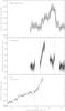 |
Fig. 14 Simultaneous X-ray, NIR and radio observations of flare I/1 from Sgr A* on 2014 Mar. 10. Top panel: the EPIC/pn smoothed light curve computed with a window width of 500 s and its error in gray. The dashed lines are the Bayesian blocks. Middle panel: the deredened HST light curve and its error in gray. The vertical dot-dashed lines are the beginning and the end of the flares. Bottom panel: the VLA light curve at 13.37 GHz. The vertical dot-dashed line is the time of the change of slope. The dashed broken line is the fit. |
The radio flare observed at 13.37 GHz (2.2 cm) could be the delayed emission from a NIR/X-ray flare that occurred either at the beginning of the observation with an amplitude lower than the detection limits of WFC3 and XMM-Newton, or before the start of our HST and XMM-Newton observations. The latter would imply a delay larger than 2.2h. As explained previously in Sect. 3.4, the largest time delay that has been measured between X-ray and sub-mm flares is 5.3 h (Yusef-Zadeh et al. 2009). Considering the expanding plasmon model (Yusef-Zadeh et al. 2006a), the delay between the X-ray and centimeter light curves must be larger than 5.3 h, and therefore the possibility of a non-detected NIR/X-ray flare is likely excluded.
4. Determination of the X-ray emission related to the NIR flares
In the following subsections we determine the X-ray emission related to each NIR flare observed with HST or VLT, with which we associate either one of the X-ray flares detected with XMM-Newton or an upper limit on the amplitude of a non-detected X-ray flare.
4.1. The NIR flare I on 2014 Mar. 10
To compare the NIR and X-ray light curves of the 2014 Mar. 10 flare, we express the NIR and X-ray flux in the same units. To convert the X-ray count rate to flux, we use the unabsorbed-flux-to-count-rate ratio derived in Sect. 3.1.3.
The NIR flux of Sgr A* is
obtained from the flux density Sν by integrating over
the F153M filter, using the filter profile T (Spanish Virtual Observatory). To be consistent
with the HST photometric calibration (Vega system), we assume a Rayleigh-Jeans regime
(Sν ∝
ν2):
 (1)with νeff the
effective frequency given by the Spanish Virtual Observatory.
(1)with νeff the
effective frequency given by the Spanish Virtual Observatory.
The ratio between the X-ray and NIR flux during the flare is shown in Fig. 15 (the error bars are on the order of the symbol size). The NIR flux is always lower than the X-ray flux, but during the third orbit of the HST visit the X-ray contribution increased by a factor of 10 compared to the NIR. We can test two interpretations: a single flare with non-simultaneous X-ray and NIR peaks, or two distinct flares with simultaneous NIR and X-ray peaks.
 |
Fig. 15 Evolution of the ratio between NIR and X-rays during flare I/1 on 2014 Mar. 10. Top panel: the dashed line surrounded by the dark gray error bars corresponds to the smoothed light curve of the X-ray flare and its flux can be seen on the left y-axis. The solid line and the light gray error bars is the NIR light curve whose flux is read on the right y-axis. Bottom panel: the flux of the X-ray light curve divided by the NIR one. |
4.1.1. A single flare with non-simultaneous peaks in NIR and X-rays
Considering that the NIR flare is produced by synchrotron emission, there are three radiative processes that can explain the X-ray flare production: synchrotron (SYN; Dodds-Eden et al. 2009; Barrière et al. 2014), inverse Compton (IC; Yusef-Zadeh et al. 2006b, 2012; Wardle 2011), and synchrotron self-Compton (SSC; Eckart et al. 2008) emission. In this section, we discuss whether each process can explain the entire observed NIR/X-ray light curve on 2014 Mar. 10.
The synchrotron−synchrotron process (SYN-SYN)
For synchrotron emission of NIR and X-ray photons by accelerated electrons in the flaring region, the electron acceleration has to be high enough to directly emit X-ray photons. It is difficult, however, to explain how to reach the required Lorentz factor of γ = 106 (Marrone et al. 2008; Yusef-Zadeh et al. 2012; Eckart et al. 2012b). Moreover, the synchrotron cooling time scale τsync = 8 × (B/ 30 G)−3/2 × (ν/ 1014 Hz)−1/2 min (Dodds-Eden et al. 2009) is very short for X-ray photons (≈ 1 s for B = 100 G and ν = 4 × 10¹⁷ Hz). Thus, we must have continuous injection of accelerated electrons to maintain the X-ray flare during the decay phase, which lasts ~30 min. If the NIR and X-ray flares are created by the same population of electrons, whose energy distribution is described by a powerlaw as N(E) = KE−p, the difference between the NIR and X-ray flux can be explained if the synchrotron spectrum has a cooling break frequency between the NIR and X-rays (Dodds-Eden et al. 2009). In this scenario, the X-ray spectrum has a spectral index of α = p/ 2, whereas the NIR spectral index is α = (p − 1)/2 (with Sν ∝ ν−α; Dodds-Eden et al. 2009). Knowing that the X-ray photons are produced by the electrons from the tail of the power law distribution, during the first part of the flare there are many more electrons that create NIR photons than those creating X-ray photons. Then, the acceleration mechanism has to become more efficient, accelerating more electrons to the tail (and thus increasing p) of the distribution and thus changing the ratio between the NIR and the X-ray flux. Hence the production of X-ray photons increases, which explains the second part of the flare.
The synchrotron−synchrotron self-Compton process (SYN-SSC)
During synchrotron self-Compton emission, X-ray photons are produced by the
scattering of the synchrotron radiation from radio to NIR on their own electron
population. If we compare the fluxes produced by the synchrotron and SSC emissions,
the variation of the X-ray/NIR ratio constrains the size evolution of the flaring
source. Let us consider a spherical source of radius R with a power law
energy distribution of relativistic electrons. Following Van der Laan (1966), the radiative transfer for the synchrotron
radiation can be computed as  (2)with κν ∝
B(p +
2)/2ν−(p +
4)/2 the absorption coefficient, ϵν ∝
B(p +
1)/2ν−(p −
1)/2 the emission coefficient, B the magnetic field
(Lang 1999) and τν(r)
the optical depth, which can be computed at each distance r from the sphere
center as:
(2)with κν ∝
B(p +
2)/2ν−(p +
4)/2 the absorption coefficient, ϵν ∝
B(p +
1)/2ν−(p −
1)/2 the emission coefficient, B the magnetic field
(Lang 1999) and τν(r)
the optical depth, which can be computed at each distance r from the sphere
center as:  (3)Assuming that we are in the optically
thin regime (i.e., τν(r) ≪
1), we utilize formula 3 of Marrone
et al. (2008): SSYN ∝ B(p +
1)/2ν−(p −
1)/2R3. For synchrotron
radiation, we have
(3)Assuming that we are in the optically
thin regime (i.e., τν(r) ≪
1), we utilize formula 3 of Marrone
et al. (2008): SSYN ∝ B(p +
1)/2ν−(p −
1)/2R3. For synchrotron
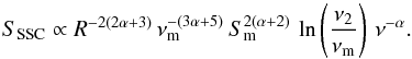
radiation, we have  with Sm the
maximum flux density of the spectral energy distribution occurring at frequency
νm (Marscher 1983). Finally, the synchrotron radiation can be expressed using
p = 2α
+ 1 as
with Sm the
maximum flux density of the spectral energy distribution occurring at frequency
νm (Marscher 1983). Finally, the synchrotron radiation can be expressed using
p = 2α
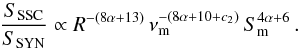
+ 1 as  (4)The SSC radiation of X-ray photons is
(formula 4 of Marscher 1983):
(4)The SSC radiation of X-ray photons is
(formula 4 of Marscher 1983):
 (5)The natural logarithm in this equation
could be approximated by c1
(ν2/νm)c2
with c1 =
1.8 and c2 = 0.201 (Eckart et al. 2012b). The synchrotron-to-SSC flux ratio is
(5)The natural logarithm in this equation
could be approximated by c1
(ν2/νm)c2
with c1 =
1.8 and c2 = 0.201 (Eckart et al. 2012b). The synchrotron-to-SSC flux ratio is
 (6)We therefore have three parameters that
may vary during the flare to explain the increased ratio of X-ray and NIR flux (Fig.
15). Considering the plasmon model, for which
a spherical source of relativistic electrons expands and cools adiabatically, we have
(Van der Laan 1966): νm ∝
R−(8α + 10)/(2α +
5) and Sm ∝ R−(14α +
10)/(2α + 5). Thus, SSSC/SSYN ∝
R−β with
β ≡
(8α2 + (30−8
c2)α + 25−10
c2)/(2α + 5). We
first consider the adiabatic expansion. For our observation, the ratio between the
X-ray and the NIR flux increases during the 2014 Mar. 10 flare, implying that
R−β must increase
as the radius R increases. This condition is satisfied if the
exponent β is negative and thus if the α value is lower than
−2.5 or is between
−2.3 and −1.25, which is inconsistent because
α must
be positive. The expansion case is thus likely to be rejected under the hypothesis of
an optically thin plasmon that expands adiabatically. We can also consider the case
where the plasmon is compressed during its motion through a bottle-neck configuration
of the magnetic field. We can still use the equations of Van der Laan (1966), since the conservation of the magnetic flux is
explicitly taken into account. The compression case is thus preferred, because it
allows positive values of α for β> 5.4. Thus, for
the SYN-SSC process, the plasmon must be adiabatically compressed with at least
SSSC/SSYN ∝
R-5.4. Therefore, the observed
increase of the X-ray-to-NIR flux ratio by a factor of 10 in 1.2 h implies a decrease
of the radius by a factor of about 0.6. The average compression velocity is estimated
as Vcomp =
ΔR/ Δt, leading to
| Vcomp |
/c< 0.0034
R/Rs with
Rs the Schwarzschild radius
(Rs = 1.2 ×
1012 cm for Sgr A*, which corresponds to 0.08 au). For
comparison, the expansion velocities computed with this model in the literature range
between 0.0028 and 0.15c (Yusef-Zadeh et
al. 2006a, 2009; Eckart et al. 2008), which is of the same order as the compression
velocity computed here. Thus, the model of an adiabatic compression of a plasmon is
the likely hypothesis to explain the variation of the ratio between X-ray and NIR
flux, in the context of the SYN-SSC process.
(6)We therefore have three parameters that
may vary during the flare to explain the increased ratio of X-ray and NIR flux (Fig.
15). Considering the plasmon model, for which
a spherical source of relativistic electrons expands and cools adiabatically, we have
(Van der Laan 1966): νm ∝
R−(8α + 10)/(2α +
5) and Sm ∝ R−(14α +
10)/(2α + 5). Thus, SSSC/SSYN ∝
R−β with
β ≡
(8α2 + (30−8
c2)α + 25−10
c2)/(2α + 5). We
first consider the adiabatic expansion. For our observation, the ratio between the
X-ray and the NIR flux increases during the 2014 Mar. 10 flare, implying that
R−β must increase
as the radius R increases. This condition is satisfied if the
exponent β is negative and thus if the α value is lower than
−2.5 or is between
−2.3 and −1.25, which is inconsistent because
α must
be positive. The expansion case is thus likely to be rejected under the hypothesis of
an optically thin plasmon that expands adiabatically. We can also consider the case
where the plasmon is compressed during its motion through a bottle-neck configuration
of the magnetic field. We can still use the equations of Van der Laan (1966), since the conservation of the magnetic flux is
explicitly taken into account. The compression case is thus preferred, because it
allows positive values of α for β> 5.4. Thus, for
the SYN-SSC process, the plasmon must be adiabatically compressed with at least
SSSC/SSYN ∝
R-5.4. Therefore, the observed
increase of the X-ray-to-NIR flux ratio by a factor of 10 in 1.2 h implies a decrease
of the radius by a factor of about 0.6. The average compression velocity is estimated
as Vcomp =
ΔR/ Δt, leading to
| Vcomp |
/c< 0.0034
R/Rs with
Rs the Schwarzschild radius
(Rs = 1.2 ×
1012 cm for Sgr A*, which corresponds to 0.08 au). For
comparison, the expansion velocities computed with this model in the literature range
between 0.0028 and 0.15c (Yusef-Zadeh et
al. 2006a, 2009; Eckart et al. 2008), which is of the same order as the compression
velocity computed here. Thus, the model of an adiabatic compression of a plasmon is
the likely hypothesis to explain the variation of the ratio between X-ray and NIR
flux, in the context of the SYN-SSC process.
The synchrotron−inverse Compton process (SYN-IC)
In the case of inverse Compton emission, X-ray photons are produced by the scattering of either the NIR photons produced by synchrotron emission from the thermal electron population associated with the accretion flow that produces the sub-millimeter photons, or the sub-millimeter photons of the accretion flow on the electron population of the external source that produces the NIR photons by synchrotron radiation.
 |
Fig. 16 NIR/X-ray peak ratio vs. time delay for the synchrotron-inverse Compton process. The asterisks are the results reported by Yusef-Zadeh et al. (2012), the solid line is a parabolic fit. The horizontal solid line and gray box are the lower limit and error bar on the NIR/X-ray peak ratio of the flare I/1 on 2014 Mar. 10 and the corresponding time-delay range. The dashed line is the ratio between the maximum NIR amplitude reported by Witzel et al. (2012) and the X-ray peak of flare 1, with the gray box being the corresponding error bar (see text for details). |
For the former process, the accretion flow is optically thin in the NIR, allowing all of the thermal electron population of the accretion flow to upscatter the NIR photons. Yusef-Zadeh et al. (2012) estimated the X-ray to NIR time delay for seven NIR/X-ray flares, which is due to upscattering of the NIR photons in the accretion flow. They identified a trend between increasing time delay and the increase of the NIR/X-ray peak ratio that is consistent with the SYN-IC process. The X-ray peak of flare 1 is defined as the maximum of the pn smoothed light curve (Table 6). We have only a lower limit on the NIR peak of flare I, which results in an estimated time delay of 25.5−73.9 min, because we have an observational gap in the HST data. Figure 16 shows a comparison of the peak ratio lower limit and time delay range of flare I/1 (horizontal solid line) with those reported in Table 2 of Yusef-Zadeh et al. (2012). This peak ratio lower limit is located below the observed trend. Assuming that the actual NIR peak can not be larger than the maximum observed amplitude (i.e., 32 mJy; Witzel et al. 2012), the actual peak ratio (dashed line) would be at least four times smaller than the value predicted by the SYN-IC process. If the actual NIR peak corresponds to this predicted value, this NIR flare would be four times brighter than the brightest flare ever observed and its shape would be completely unusual. We therefore consider this process to be very unlikely.
For the latter process, the accretion flow is optically thick in sub-millimeter, reducing the number of available sub-millimeter photons produced by the thermal electron population to be upscattered (Yusef-Zadeh et al. 2006b, 2012; Wardle 2011). If the sub-millimeter flux of the accretion flow is constant, the X-ray flare should have the same shape as the NIR flare. But in flare I/1 the X-ray flux increases while the NIR flux decreases. Since the decay of the NIR flux can only be due to the decrease of the number of accelerated electrons, the rise of the X-ray flux would require a simultaneous large increase of the sub-millimeter flux, which appears rather fine tuned. Therefore, we do not favor the SYN-IC process to explain the variation of the NIR/X-ray flux of flare I/1.
4.1.2. Two distinct flares with simultaneous NIR and X-ray peaks
The 2014 Mar. 10 flare could be decomposed into two flaring components (called Ia/1a
and Ib/1b). Each NIR/X-ray flaring component is produced by its own population of
accelerated electrons. We introduce here a general model that will be used in the next
subsections to fit the NIR and X-ray light curves. The model is composed of a linear
part (if needed), representing the non-flaring level, plus one or two Gaussian flares:
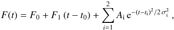 (7)with Ai the
amplitude above the non-flaring level and ti and σi the center
and the standard deviation of each Gaussian. For the X-rays, the non-flaring level is
fixed to the Bayesian-block value. The results of the fit are given in Table 8 and the corresponding light curves and residuals
are shown in Fig. 17 (top panels).
(7)with Ai the
amplitude above the non-flaring level and ti and σi the center
and the standard deviation of each Gaussian. For the X-rays, the non-flaring level is
fixed to the Bayesian-block value. The results of the fit are given in Table 8 and the corresponding light curves and residuals
are shown in Fig. 17 (top panels).
The time of the first and second peaks of the NIR and X-ray flares are consistent with each other within the 1σ errors. Flare 1b appears broader in X-rays than in the NIR, but their widths are consistent with each other within 1.5σ. The delay time between the two X-ray maxima is about 5000 s, which is longer than the time between two X-ray flares observed during the 2012 Chandra XVP campaign (about 4000 s; see Fig. 1 of Neilsen et al. 2013). This argument, in addition to the change of flux ratio between the two flares, favors the interpretation of two distinct flares.
From the unabsorbed-flux-to-count-rate ratio derived in Sect. 3.1.3, we compute the unabsorbed total energy of these flares using the total number of counts in each Gaussian. The start and stop times of the flares are defined as the 3σ distance from the time of the maximum, i.e., 16.0 and 17.6 h for flare 1a, and 17.4 and 19.8 h for flare 1b. The unabsorbed total energy is (12.7 ± 6.7) × 1037 and (21.2 ± 6.5) × 1037 ergs (1σ error) for flares 1a and 1b, respectively. The unabsorbed total energy of flare 1 is thus split nearly equally between its two components. The peak amplitude of flare 1a is close to the smallest amplitudes of flares observed (Fig. 8).
Gaussian fitting of the NIR and X-ray flares observed during the 2014 campaign.
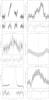 |
Fig. 17 Light curve fitting of the HST NIR flares (left panels) and the X-ray (right panels) counterparts. The solid lines are the observed light curves with the error bars in gray. The dashed lines in right panels are the Bayesian blocks. The X-ray light curves are smoothed with a window width of 500 s and 100 s for 2014 Mar. 10 and Apr. 2, respectively. The dotted lines are the individual Gaussians and the dot-dashed line is the sum of the Gaussians. The vertical dotted lines are the time of the NIR flare peak when there is no detected X-ray counterpart. The residuals are in units of σ. |
4.2. The NIR flare II on 2014 Mar. 10
This flare is only detected in the NIR with HST. We therefore fit the NIR light curve with a single Gaussian above a constant non-flaring level using Eq. (7). The best fit parameters are reported in Table 8.
The upper limit on the amplitude of the undetected X-ray counterpart was computed using the Bayesian method for the determination of the confidence limits described by Kraft et al. (1991, see also Helene 1983. We use the notations and equations of Sect. 3.1.2. We first define a confidence limit CL = 0.95 and the source N as the number of counts during the time interval of the flare maximum (i.e., between ti − 3σ and ti + 3σ with σ the error on ti reported in Table 8). The background B is the number of counts in the non-flaring Bayesian-block at the time of the NIR flare peak. We then determine smin and smax (see footnote 5 in Sect. 3.1.2) resolving the equation of CL. For flare II, N = 62 counts and the non-flaring level is defined by the Bayesian blocks as 0.315 counts s-1 between 21.65 and 21.71 h, leading to B = 68 counts and S = −6 counts. Since S is negative, smin = 0, leading to smax = 6. The upper limit on the amplitude is thus 0.028 counts s-1 at a confidence level of 95%. The value of this upper limit is also reported in Table 8.
4.3. The NIR flare III on 2014 Apr. 2
We consider that two NIR flares happened during the occultation of Sgr A* by the Earth. We thus fit the NIR light curve with two Gaussians (labeled IIIa and IIIb) above a linear component, which is used here to take into account the change in the non-flaring level between the last two HST orbits (Eq. (7)). The F-test strongly supports two Gaussian components, since this significanlty increases the goodness-of-fit (p-value of 3 × 10⁻⁴). The best-fit parameters for the X-ray and NIR flares are given in Table 8 and the resulting graphs are shown in the bottom panels of Fig. 17.
We then fit the X-ray flare 2 with a Gaussian above a quiescent level equal to the Bayesian-block value. The maximum of the X-ray flare has no time delay relative to the NIR flare IIIa above the 3σ error bars, as usually observed for X-ray flares with NIR counterparts (Eckart et al. 2006; Yusef-Zadeh et al. 2006a; Dodds-Eden et al. 2009). Moreover, the FHWM of the NIR flare IIIa (2458 s) is about 3 times larger than that of the X-ray flare (762 s), which is reminiscent of the FWHM ratio of ~2 observed by Dodds-Eden et al. (2009) for the 2007 Apr. 4 NIR/X-ray flare. The NIR flare IIIa is thus probably the counterpart of the X-ray flare 2. This conclusion is based on our Gaussian fitting of flare III, but a more complex shape cannot be excluded due to the NIR observational gap. However, since the X-ray flare 2 and the previously observed NIR/X-ray flares also have a Gaussian shape (Eckart et al. 2006; Yusef-Zadeh et al. 2006a; Dodds-Eden et al. 2009), we consider that this conclusion is the simplest and thus the most likely.
The amplitude of the flare IIIb is one of the largest observed when compared with the sample obtained with NACO (Witzel et al. 2012). No X-ray counterpart is detected for this flare. We thus obtain an upper limit on the X-ray amplitude using the same method as flare II with N = 763 counts between 16.9 and 17.5 h. The background is defined as the sum of the number of counts in non-flaring Bayesian-block values (626.4 counts) and the number of counts in the Gaussian fit of flare 2 during the maximum of the flare (121.7 counts). We thus have B = 748.1 counts, leading to S = 14.9 counts. The resulting smin is 0, with smax = 65 counts. The upper limit on the amplitude of the undetected X-ray counterpart is thus 0.030 counts s-1 at the confidence level of 95%. This value is reported in Table 8.
4.4. The NIR flare IV on 2014 Apr. 3
The VLT light curves consist of bins of 400 s exposures. The number of bins is too small and the bin size too large to fit a Gaussian to the VLT light curves. We thus consider only the bin with the largest flux density as the peak of the flare IV. This value and the time of the maximum are reported in Table 8.
No X-ray counterpart is detected with XMM-Newton on Apr. 3. We thus deduce an upper limit to the putative simultaneous X-ray flare using the same method that was used for flare II. The time interval of the maximum of flare IV is defined as the bin length of the light curve, i.e., 400 s centered on 7.89 h. The number of counts in this interval is N = 127 counts and the background is B = 119.1 counts, leading to S = 7.9 counts. The resulting smin is 0, with smax = 17 counts, leading to an upper limit on the amplitude of 0.042 counts s-1.
4.5. The NIR flare V on 2014 Apr. 4
For flare IV, we do not fit the light curve with a Gaussian and we consider the maximum of the light curve as the peak flux density of the NIR flare (Table 8).
We have no XMM-Newton observation on 2014 Apr. 4. However, as shown in
Fig. 1, there is a simultaneous legacy
Chandra observation (ObsID: 16212; PI: D. Haggard) on this date. We
used the Chandra Interactive Analysis of Observations (CIAO; version 4.6)
to analyze these data. We worked with the level = 2 event list of the ACIS-S
camera (Garmire et al. 2003), available in
the primary package of the Chandra archive. We extracted the
source+background events in the 2−8 keV energy range in a 125-radius
circle centered on the radio coordinates of Sgr A* using the dmcopy
task. We used the Bayesian-blocks analysis with a false detection probability
of e-3.5 to detect
any flaring event. No X-ray counterpart to the NIR flare was detected during this
observation. Based on N =
1 counts between 8.71 and 8.93 h and a non-flaring level of
0.0065 counts
s-1, we compute B = 3 counts and S = −2 counts. The
resulting smin is 0 with smax = 4 counts.
The upper limit to the putative simultaneous X-ray amplitude is thus 0.01 counts s-1 at the confidence
level of 95% (see flare II for explanations).
5. Constraining the physical parameters of the flaring region
In this section we constrain the physical parameters of the flaring region by considering three radiative models for the NIR and X-ray emission. After computing the NIR-to-X-ray simultaneous peak ratio sample detected during the 2014 campaign, we investigated the synchrotron-synchrotron (SYN-SYN), synchrotron Self-Compton-synchrotron Self-Compton (SSC-SSC), and the synchrotron-synchrotron Self-Compton (SYN-SSC) radiation mechanisms. These processes are called “local”, because these emissions are produced only by the electrons accelerated in the flaring region. The last subsection is dedicated to the Inverse Compton mechanism, which involves external electrons.
5.1. The sample of NIR flares and the corresponding X-ray emission
We compute the flux densities of the NIR and X-ray flare peaks to constrain the physical parameters of the flaring region needed to produce such fluxes. We extrapolate the amplitude of each NIR peak to the Ks-band using the H − L spectral index computed in Witzel et al. (2014b). The flux density of the X-ray flare peaks is computed from the spectral fitting in ISIS, using the typical spectral parameters of the X-ray bright flares (see Sect. 3.1.3). The resulting conversion factor is 1 pn count s-1 = 3.935μJy at 4 keV. The NIR peak flux density and corresponding values of the X-ray peaks (or upper limits) are reported in Table 8.
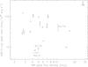 |
Fig. 18 NIR-to-X-ray peak ratio vs. amplitude of the NIR flares. Squares refer to the flares reported in Table 3 of Eckart et al. (2012b). Triangles are the simultaneous NIR/X-ray flares detected on 2007 Apr. 4 and labeled D and E in Table 2 of Trap et al. (2011). Diamonds are the delayed flares of 2004 Jul. 7, 2008 Jul. 26+27 and 2008 May 5 reported in Table 2 of Yusef-Zadeh et al. (2012). The labeled points are the NIR and X-ray flares observed during this campaign. |
Figure 18 shows the NIR-to-X-ray peak ratio as a function of the amplitude of the NIR flares observed during the 2014 campaign. The unabsorbed X-ray peak luminosities are computed using the conversion factor reported in Sect. 3.1.3. The X-ray upper limit of NIR flare V was obtained from Chandra data. The corresponding unabsorbed-flux-to-count-rate ratio of 1.97 × 10⁻¹⁰ erg s-1 cm-2/ count s-1 was computed with the same spectral parameters as for XMM-Newton.
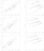 |
Fig. 19 Physical parameters of the flares observed simultaneously in X-rays and NIR for the three emission models. The flare Ia/1a, Ib/1b and IIIa/2 are in the upper, middle and bottom panels, respectively. Left panels are the size of the flaring-source region (θ) vs. the peak of the spectrum (Sm) at the frequency νm. Right panels are the density of the relativistic electrons vs. the magnetic field. The locii where the Synchrotron Self-Compton−Synchrotron Self-Compton (SSC-SSC), Synchrotron-Synchrotron Self-Compton (SYN-SSC) and Synchrotron-Synchrotron (SYN-SYN) are dominant are shown in black, blue and green, respectively. The red dots represent the turnover frequencies from 50 to 3000 GHz by step of 200 GHz. The arrows show the direction of the curves if the limit on the alternative emission processes is lowered. Dotted lines are locii of SYN-SSC where the MIR emission is larger than the observed upper-limit values (see text for details). |
We also show the flares reported by Eckart et al. (2012b), the two simultaneous flares on 2007 Apr. 4 (Porquet et al. 2008; Nowak et al. 2012) labeled D and E in Table 2 of Trap et al. (2011), and the delayed flares of 2004 Jul. 7, 2008 Jul. 26+27, and 2008 May 5 reported in Table 2 of Yusef-Zadeh et al. (2012).
The flare Ia/1a lies within the bulk of NIR flare amplitudes and peak ratio, whereas the flare IIIa/2 has the lowest NIR-to-X-ray ratio ever observed. The NIR flare IIIb is amongst the largest NIR flares (e.g., Dodds-Eden et al. 2009; Witzel et al. 2012) and has the largest NIR-to-X-ray ratio ever observed.
5.2. Investigation of the local radiative processes
With the peak flux density of the flares in X-rays and NIR, we use the formalism developed by Eckart et al. (2012b) to constrain the range of four physical parameters of the flaring emission: the size of the source region, the magnetic field, the density, and the maximum of the flux density spectrum. Eckart et al. (2012b) considered three cases, invoking the two radiative processes, implying the local electrons from the flaring source region: the SYN-SYN, SSC-SSC, and SYN-SSC emissions. A radiative process is considered as dominant when the alternative emission processes are lower than 10%. For example, the SYN-SYN case is dominant if both SSC contribution for NIR and X-rays are lower than 10% of the synchrotron contribution. Considering different values for the turnover frequency (νm), which defines the frequency at which the source becomes optically thin, we have four free physical parameters for each value of the spectral index (α): the size of the emitting region (θ), peak flux density at νm (Sm), number density of relativistic particles (ρ), and the magnetic field (B). The spectral index is given by the ratio between the NIR and X-ray amplitudes for the SYN-SYN and SSC-SSC cases, and by seven different values of α from 0.3 to 1.5 for the SYN-SSC case. Computing the SYN or SSC flux density with the equations given by Eckart et al. (2012b), we can constrain the values of the four physical parameters for each value of α and νm.
The resulting graphs for the flares detected in NIR and X-rays (labeled Ia/1a, Ib/1b and IIIa/2) are shown in Fig. 19. Each line corresponds to one value of α. The red dots are the turnover frequencies from 50 to 3000 GHz in steps of 200 GHz. The constraint on the MIR amplitude limit observed during the bright L′-band and X-ray flare on 2007 Apr. 4 of 57 mJy at 11.88 μm (Dodds-Eden et al. 2009) is also used: the lines are dashed if this limit is exceeded. This happens only for the SYN-SSC emission mechanism and for high values of α.
The physical parameters are more constrained for flare IIIa/2, since the X-ray-to-NIR amplitude ratio is high. For this flare, the SYN-SSC emission mechanism leads to a size of 0.03−7 times the Schwarzschild radius and an electron density of 108.5–1010.2 cm-3 for a synchrotron spectral-index of 0.3−1.5.
From the magnetic field values deduced for these flares, one can infer the presence of sustained heating during the decay phase of the X-ray or NIR flares for the SYN-SYN and SYN-SSC case. Indeed, if the synchrotron cooling timescale, defined as τsync = 8(B/ 30 G)−3/2(ν/ 1014 Hz)−1/2 min (Dodds-Eden et al. 2009), is shorter than the duration of the decay phase then sustained heating is needed. We define the decay phase from the time of the maximum of the Gaussian fit (see Table 8) to the time leading to 10% of the flare amplitude (corresponding to 2.1σ after the maximum) in order to still have a detectable emission of the flare.
For the SYN-SYN case, the synchrotron cooling timescale is shorter for the X-ray photons, leading to more constraints on the presence of sustained heating. We thus consider the X-ray frequency (ν = 1018 Hz) in the computation of the synchrotron cooling timescale. The synchrotron cooling timescale is shorter than the decay time of flare 2 (695 s) for B larger than 1 G, implying that sustained heating must be present during the decay phase for these values of magnetic field. A sustained heating is always needed for flares Ia/1a and Ia/1b, since they have a minimum value of the magnetic field and a decay time larger than those of flare 2 (2318 and 2781 s, respectively).
For the SYN-SSC case, we consider the NIR frequency (ν = 1014 Hz) in τsync that we have to compare to the decay time of the NIR flares. Sustained heating is now needed for flare IIIa (whose decay time is 2240 s) with a magnetic field of greater than 11 G, corresponding to an electron density larger than 1010.1 cm-3. For flares Ia and Ib (whose decay times are 1545 and 3785 s, respectively), sustained heating is needed for magnetic fields larger than 13 and 7 G, respectively. The corresponding electron density is thus larger than 108.4 and 109.5 cm-3.
We also apply the study of Eckart et al. (2012b) to constrain the physical parameters of the flaring emission for the NIR flares that have no detected X-ray counterpart (flares II, IIIb, IV and V). The resulting graphs are shown in Fig. 20. The necessary electron density and magnetic field ranges lie within lower values compared to those needed to produce detectable X-ray flares, since the efficiency of the production of X-ray photons is smaller. Moreover, for flare IIIb, the SYN−SYN process is only dominant for small values of νm. This is explained by the small X-ray-to-NIR amplitude ratio, since at large νm the synchrotron process is too efficient for the production of a small number of X-ray photons.
We can also deduce the presence of sustained heating during the decay phase of NIR flares II and IIIb for the SYN-SYN and SYN-SSC case. The synchrotron cooling timescale is shorter than the decay time of flare II (772 s) if B is larger than 22 G, requiring sustained heating during the decay phase for these values of magnetic field. For flare IIIb (whose decay times are 695 s), sustained heating is required for B larger than 1 G.
However, as argued by Eckart et al. (2012a), alternative models such as different spectral indexes for the NIR and X-ray, due to inhomogeneities of the accretion disk, can also explain the data with larger numbers of free parameters.
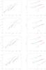 |
Fig. 20 Physical parameters of the flares only observed in NIR for the three emission models. The NIR flare II, IIIb, IV and V are in the upper, second, third and bottom panels, respectively. See Fig. 19 caption for the panel description. |
5.3. Investigation of the external radiative process
As reported in Sect. 4.1.1, Yusef-Zadeh et al. (2012) investigated the upscattering of the NIR
photons produced in the flaring region on electrons of the accretion flow. The ratio
between the Inverse Compton and the synchrotron emission is
 (8)with Uph the photon
energy density and UB = B2/
8π the magnetic energy density. Given the variation of
B with the
distance from Sgr A*
(B =
B0
(r/Rs)-1 with
B0 of several hundred of Gauss; Eatough et al. 2013), it is possible to create NIR and
X-ray flares with a large range of NIR-to-X-ray ratio. Thus, we cannot identify the IC
radiation by only considering the NIR-to-X-ray ratio.
(8)with Uph the photon
energy density and UB = B2/
8π the magnetic energy density. Given the variation of
B with the
distance from Sgr A*
(B =
B0
(r/Rs)-1 with
B0 of several hundred of Gauss; Eatough et al. 2013), it is possible to create NIR and
X-ray flares with a large range of NIR-to-X-ray ratio. Thus, we cannot identify the IC
radiation by only considering the NIR-to-X-ray ratio.
However, using the estimation of the time delay between X-ray and NIR flare peaks as a function of the NIR-to-X-ray peak ratio reported in Yusef-Zadeh et al. (2012) and shown in Fig. 16, we can estimate the time delays that we would observe during our 2014 campaign. For the detected X-ray flares, the NIR-to-X-ray peak ratio ranges between 6 and 45 mJy/1035 erg s-1 (see Fig. 18) leading to a time delay less than 10 min, which is smaller than the error bars on the time of the maximum of the Gaussians. The IC emission, therefore, is still a possible radiative process for the production of the X-ray flares observed during this campaign.
For the undetected X-ray flares II, IIIb, IV and V, the NIR-to-X-ray ratio is larger than 32, 269, 48, and 55 mJy/1035 erg s-1, respectively. The corresponding time delays are thus greater than 9, 26, 11, and 12 min, respectively. These time delays are larger than the events with detected X-ray flares. The efficiency of the flare detection with XMM-Newton and Chandra, however, does not allow us to detect such faint X-ray flares, which may have the largest delay in the inverse Compton framework.
Thus, the flares observed during the 2014 campaign leave the IC process as a possible emission mechanism for producing X-ray flares from the NIR photons.
6. Discussing the X-ray flaring rate
We can compare the X-ray flare frequency during our observations (three flares over 255.644 ks) to the one derived from the Chandra XVP campaign in 2012: 45 flares detected by Bayesian-block algorithm over 2983.93 ks (1.5 flare per day). Considering a sample of 45 flares having the same amplitude and duration distribution as those observed during the Chandra XVP campaign superimposed on the non-flaring level observed with XMM-Newton during our campaign, the Bayesian-blocks algorithm detects 36 flares over 2983.93 ks. If we sum the number of flares that we can detect during the exposure time corresponding to each observation during the XMM-Newton 2014 campaign, we arrive at a prediction of 3.1 flares during this campaign. We compare the flare rate observed during the Chandra XVP campaign to those observed during this campaign (36 flares over 2983.93 ks and 3 flares over 255.644 ks), assuming a Poisson process (Gehrels 1986; Fay 2010). The p-value for the null hypothesis that the flaring rate we have to observe and the rate we currently observe is the same, is 1, which implies that the flaring rate observed close to the pericenter passage of the DSO/G2 is consistent with that observed during the Chandra XVP campaign. The conclusion is the same if we consider only two X-ray flares instead of three (p-value = 0.54). To conclude that the measured flaring rate is statistically different from those observed during the Chandra XVP campaign, we would have to detect at least 8 flares during our campaign (p-value = 0.04), which corresponds to an increase of the flaring rate by a factor of 2.6 (95% confidence interval of 1.0−5.7).
Since the beginning of the observation of Sgr A* in X-rays, two temporary episodes of higher flaring rate were observed (Porquet et al. 2008; Neilsen et al. 2013). Porquet et al. (2008) detected four flares on 2007 Apr. 04 with XMM-Newton. Three of these flares happened during the last 39.6 ks of the observation, corresponding to a flaring rate of 8.8 flares per day. We can compare this flaring rate to the 38 flares that should be detected by the Bayesian-block algorithm. The ratio between the two rates is 5 and the 95% confidence interval is 1.3−20 (p-value = 0.03). Neilsen et al. (2013) detected 4 flares during 23.6 ks with Chandra, which corresponds to a flaring rate of 14.6 flares per day. We can directly compare this flaring rate to that computed during the 2012 Chandra XVP campaign if we remove these 4 flares from the sample of 45 flares detected by the Bayesian-blocks algorithm. Thus, we have to compare 41 flares over 2960.33 ks and 4 flares over 23.6 ks. The ratio between the two rates is 13 and the 95% confidence interval is 3.3−33.3 (p-value = 9 × 10⁻⁴). This implies that some temporary increase of Sgr A* activity in X-ray may have been observed without an increase of the quiescent level due to an increase of the accretion rate.
The radio monitoring of Sgr A* with VLA between 2012 and 2014 May showed no change in the flux density or the spectrum (Bower et al. 2015a; Yusef-Zadeh et al. 2015). Observations of Sgr A* after the DSO/G2 pericenter passage show that there is no increase of the flaring activity in radio/sub-mm (Tsuboi et al. 2015; Park et al. 2015). The 2014 Feb.−June Chandra X-ray monitoring of Sgr A* shows no rise of the quiescent flux (Haggard et al. 2014). The compactness of the object can explain the absence of any increase in the Sgr A* accretion rate during pericenter passage at 2014.39 ± 0.14 (Valencia-S. et al. 2015), which corresponds to 2014 Apr. 20 (2014 Mar. 1−2014 Jun. 10). Five flares with an absorbed fluence greater than 5 × 10⁻⁹ erg cm-2 (corresponding to an unabsorbed fluence of 10.9 × 10⁻⁹ erg cm-2 when using Γ = 2 and NH = 14.3 × 1022 cm-2) were observed with XMM-Newton and Chandra between 2014 Aug. 30 and Oct. 20, implying an increase in the rate of energetic flares, but the overall flaring rate did not change (Ponti et al. 2015).
To assess the typical timescale for the accretion of fresh matter from the DSO/G2 object onto Sgr A* at pericenter, we compute the disk accretion timescale (τacc) for Sgr A*. It is governed by the viscous timescale, which is computed for an ADAF using the self-similar solution derived by Yuan & Narayan (2014, and references therein). At the distance r of the SMBH, τacc is defined as r/Vrad with Vrad the radial velocity for the self-similar solution, which gives us: τacc ~ 3.0 (r/ 2000Rs)1.5 (α/ 0.1)-1 yrs with α ∈ [ 0,1 ] the efficiency of the mechanism of angular momentum transport introduced by Shakura & Sunyaev (1973). For a pericenter distance of about 2000 Rs (Pfuhl et al. 2015; Valencia-S. et al. 2015) and α = 0.1, we should not see any increase of the flux from Sgr A* before 2017. Moreover, the large angular momentum of the gas and dust from DSO/G2 likely increases the true accretion timescale.
Some numerical simulations of the accretion of gas in a RIAF model were made, leading to a time range for the gas accretion of some months to several ten of years after the pericenter passage (Burkert et al. 2012; Schartmann et al. 2012). However, these simulations modeled DSO/G2 as a gas cloud or a spherical shell of gas, but not as a young star with circumstellar material. The accretion time when there is no central star may thus be lower than τacc, since the gas cloud is partially tidally disrupted before the pericenter passage.
Zajaček et al. (2014) modeled the DSO/G2 as an intermediate mass star of 2 M⊙ moving in a RIAF. They studied the tidal effects on a circumstellar dusty envelope and on a circumstellar accretion disk. They showed that if the test particles are distributed in a disk-like structure, the number of particles that remain gravitationally bound to the star after the pericenter passage is larger than that for a spherical distribution of particles. From their Fig. 13, we can also infer that the accretion onto Sgr A* begins earlier for a spherical distribution than for a disk-like model. However, in these simulations, no circumstellar gas was taken into account.
7. Conclusions
The pericenter passage of the DSO/G2 object at the beginning of 2014 was predicted to produce an increase of the flaring activity of Sgr A* in several wavelengths. This 2014 Feb.−Apr. campaign was designed to follow an increase of its flaring activity simultaneously in X-rays, NIR, and radio/sub-mm.
Three NIR flares were detected with WFC3 on board HST: two on 2014 Mar. 10 (I and II) and one on Apr. 2 (III). Two additional NIR flares were detected with SINFONI at ESO’s VLT on 2014 Apr. 3 (IV) and 4 (V). All of these NIR flares are within the top 8% of the largest amplitude flares observed with NACO at ESO’s VLT (Witzel et al. 2012). Since the detection limit of WFC3 and SINFONI correspond to the 8 and 11% amplitude levels of this sample, the fact that the observed NIR flares belong to the most luminous NIR flares is statistically expected and can not be taken as any indication for an increase of NIR activity.
Two X-ray flares were detected on 2014 Mar. 10 (1) and Apr. 2 (2) using the Bayesian-blocks method on the XMM-Newton observations. The spectral parameters of these X-ray flares fitted with the MCMC method are consistent with those of the two brightest flares detected with XMM-Newton (Porquet et al. 2003, 2008).
The flare I/1 observed on 2014 Mar. 10 presents a change in the NIR to X-ray flux ratio, with an increase of the X-ray flux contribution during the second half of the flare. We tested the three radiative processes that can explain the NIR/X-ray flares from Sgr A* as a single flare, considering energetic arguments. The most likely interpretation is that the NIR and X-ray photons are produced in a plasmon in adiabatic compression by synchrotron and SSC emission mechanisms, respectively. However, the flares I and 1 can also be decomposed into two Gaussian flares with a time separation of only 1.2 h. We can thus associate the NIR flares Ia and Ib to the X-ray flares 1a and 1b, respectively. They reproduce the characteristics observed in other simultaneous NIR/X-ray flares, i.e., no apparent delay between the maxima and a similar FWHM. The flares Ia/1a lie within the bulk of NIR flare amplitudes and peak ratio, but the flare Ib/1b lies within the lowest peak ratio ever observed.
The NIR flare III is actually composed of two close Gaussian flares (IIIa and IIIb). The X-ray flare 2 is the counterpart of the NIR flare IIIa. It has the lowest NIR-to-X-ray ratio ever observed.
The NIR flares II, IIIb, IV, and V have no detectable X-ray counterpart in our XMM-Newton observation or the legacy Chandra observation. The upper limits on the X-ray amplitude were computed using the Bayesian method for the determination of the confidence limits described by Helene (1983) and Kraft et al. (1991). The flare IIIb lies within the largest NIR fluxes (e.g., Dodds-Eden et al. 2009; Witzel et al. 2012) and has the largest NIR-to-X-ray ratio ever observed.
In total, we detected seven NIR flares and three X-ray flares during the 2014 campaign.
On 2014 Mar. 10 we also identified an increase in the rising radio flux density at 13.37 GHz with the VLA, which could be the delayed radio emission from a NIR/X-ray flare that occurred before the start of our observation.
On 2014 Apr. 2 we identified a bump of the flux density on the rising 3.2-mm light curve observed with CARMA. The time range of this observation does not allow us to associate this millimeter bump to a NIR/X-ray flare. Moreover, we found no significant delay between the CARMA light curve and VLA L- and C-band data.
On 2014 Apr. 3 two millimeter flares were identified above the decaying 3.2-mm light curve. The former could be the delayed emission of the NIR flare IV.
We derived physical parameters of the flaring emission for local radiative processes, as done previously by Eckart et al. (2012b), for each NIR/X-ray flare, and also for NIR flares with no detected X-ray counterpart. Physical parameters for the flare IIIa/2 are better constrained when asssuming synchrotron and SSC emission mechanisms for the NIR and X-ray flares, respectively. This flaring region has a size of 0.03−7 times the Schwarzschild radius and an electron density of 108.5–1010.2 cm-3, for a synchrotron spectral-index of 0.3−1.5. The derived physical parameters of the flaring emission associated with the undetected X-ray counterpart are poorly constrained, since the X-ray photon production efficiency is smaller.
We also tested the SYN-IC process using the NIR-to-X-ray peak amplitude ratio and the predicted time delay between the NIR and X-ray peaks. This external radiative process is also a possible emission model for the emission of the flares observed during this campaign.
No significant increase in the X-ray flaring rate has been detected during this campaign, but continuous monitoring of Sgr A* is still important to detect any steady increase of its flaring activity that could be due to accreting material from the DSO/G2. This may put some constrains on the physical properties of the G2 object and the ambient medium inside the Bondi radius of this SMBH.
The website of xTime is: http://heasarc.gsfc.nasa.gov/cgi-bin/Tools/xTime/xTime.pl
Worpel & Schwope (2015) tested different photon-weighting in order to subtract the background during observations of bursting and eclipsing objects in X-rays. The equation for the Voronoi time-interval weighting used in Mossoux et al. (2015a,b) follows the recipe of Scargle et al. (2013b), which is identical to the “alternative” photon-weighting described in Sect. 4.6 of Worpel & Schwope (2015) since the photon-weighting is equal to the inverse of the Voronoi time-interval weighting. We can see in Fig. 12 of Worpel & Schwope (2015) that the method of Mossoux et al. (2015a,b) (labeled h in this figure) locates the eclipses, as well as their weighted-photon method (labeled f in this figure). As noticed by Worpel & Schwope (2015), their weighted-photon method may produce both negative and implausibly high count rates. Indeed, the method of Mossoux et al. (2015a,b) produces much fewer Bayesian blocks with negative count rates and no implausibly high count rates in comparison to their weighted-photon method (see for comparison panel h and f of Fig. 12 of Worpel & Schwope 2015). This last point is crucial for flare and burst detection.
The website of the Spanish Virtual Observatory is: http://svo.cab.inta-csic.es/main/index.php
For comparison, the FWHM of the NICMOS Camera 1 is
 (3.75 detector pixels) at 1.60
μm (Yusef-Zadeh et al. 2006b), i.e., better sampled than
the FWHM of the WFC3 camera.
(3.75 detector pixels) at 1.60
μm (Yusef-Zadeh et al. 2006b), i.e., better sampled than
the FWHM of the WFC3 camera.
Following Kraft et al. (1991), we first determine
the confidence interval [smin, smax] of
S ≡ N −
B at the confidence level CL where, for a count
excess, smax is defined as fN,B(smax) ≡
fN,B(smin)
and smin =
0, with  is the posterior probability distribution
function. We then compute
is the posterior probability distribution
function. We then compute  and its Gaussian equivalent in units of
σ given by
φ-1((1 −
CL)/2), with φ-1 being the
reciprocal of the cumulative distribution function of the normal distribution.
and its Gaussian equivalent in units of
σ given by
φ-1((1 −
CL)/2), with φ-1 being the
reciprocal of the cumulative distribution function of the normal distribution.
The equation computing the signal-to-noise ratio is the same as in specgroup and in ISIS (Houck 2013). We therefore use the same grouping as in Mossoux et al. (2015a).
The cutoff value is given as a lower limit in Neilsen et al. (2013) but the specific value does not influence the result of our flare distribution because we are interested by flares characterized by small amplitude and short duration since these flares may suffer of the small detection rate.
Acknowledgments
This work has been financially supported by the Programme National Hautes Énergies (PNHE). The research leading to these results has received funding from the European Union Seventh Framework Program (FP7/2007-2013) under grant agreement No. 312789. The XMM-Newton project is an ESA Science Mission with instruments and contributions directly funded by ESA Member States and the USA (NASA). This work is based on observations made with the NASA/ESA Hubble Space Telescope obtained at the Space Telescope Science Institute, which is operated by the Association of Universities for Research in Astronomy, Inc., under NASA contract NAS 5-26555. These HST observations are associated with programs 13403 and 13316. This work is based on observations made with ESO Telescopes at the Paranal Observatory under programs 091.B-0183(H), 092.B-0920(A) and 093.B-0932(A). Karl G. Jansky Very Large Array (VLA) of the National Radio Astronomy Observatory is a facility of the National Science Foundation, operated under a cooperative agreement by Associated Universities, Inc. Support for CARMA construction was derived from the states of California, Illinois, and Maryland, the James S. McDonnell Foundation, the Gordon and Betty Moore Foundation, the Kenneth T. and Eileen L. Norris Foundation, the University of Chicago, the Associates of the California Institute of Technology, and the National Science Foundation. Ongoing CARMA development and operations are supported by the National Science Foundation under a cooperative agreement, and by the CARMA partner universities.
References
- Alexander, T. 1997, in Astronomical Time Series, eds. D. Maoz, A. Sternberg, & E. M. Leibowitz, Astrophys. Space Sci. Libr., 218, 163 [Google Scholar]
- Baganoff, F. K., Bautz, M. W., Brandt, W. N., et al. 2001, Nature, 413, 45 [NASA ADS] [CrossRef] [PubMed] [Google Scholar]
- Baganoff, F. K., Maeda, Y., Morris, M., et al. 2003, ApJ, 591, 891 [NASA ADS] [CrossRef] [Google Scholar]
- Barrière, N. M., Tomsick, J. A., Baganoff, F. K., et al. 2014, ApJ, 786, 46 [NASA ADS] [CrossRef] [Google Scholar]
- Bonnet, H., Abuter, R., Baker, A., et al. 2004, The Messenger, 117, 17 [NASA ADS] [Google Scholar]
- Bower, G. C., Deller, A., Demorest, P., et al. 2015a, ApJ, 798, 120 [NASA ADS] [CrossRef] [Google Scholar]
- Bower, G. C., Markoff, S., Dexter, J., et al. 2015b, ApJ, 802, 69 [NASA ADS] [CrossRef] [Google Scholar]
- Brinkerink, C. D., Falcke, H., Law, C. J., et al. 2015, A&A, 576, A41 [NASA ADS] [CrossRef] [EDP Sciences] [Google Scholar]
- Burkert, A., Schartmann, M., Alig, C., et al. 2012, ApJ, 750, 58 [NASA ADS] [CrossRef] [Google Scholar]
- Coti Zelati, F., Rea, N., Papitto, A., et al. 2015, MNRAS, 449, 2685 [NASA ADS] [CrossRef] [Google Scholar]
- Cotton, W. D. 2008, PASP, 120, 439 [NASA ADS] [CrossRef] [Google Scholar]
- Degenaar, N., Reynolds, M., Miller, J. M., Kennea, J., & Wijnands, R. 2013, The Astronomer’s Telegram, 5006, 1 [NASA ADS] [Google Scholar]
- Dodds-Eden, K., Porquet, D., Trap, G., et al. 2009, ApJ, 698, 676 [NASA ADS] [CrossRef] [Google Scholar]
- Dressel, L. 2012, Wide Field Camera 3 Instrument Handbook for Cycle 21 v. 5.0 (Baltimore: STScI) [Google Scholar]
- Eatough, R. P., Falcke, H., Karuppusamy, R., et al. 2013, Nature, 501, 391 [NASA ADS] [CrossRef] [PubMed] [Google Scholar]
- Eckart, A., & Duhoux, P. R. M. 1991, in ASP Conf. Ser. 14, ed. R. Elston, 336 [Google Scholar]
- Eckart, A., Baganoff, F. K., Schödel, R., et al. 2006, A&A, 450, 535 [NASA ADS] [CrossRef] [EDP Sciences] [Google Scholar]
- Eckart, A., Schödel, R., García-Marín, M., et al. 2008, A&A, 492, 337 [NASA ADS] [CrossRef] [EDP Sciences] [Google Scholar]
- Eckart, A., García-Marín, M., Vogel, S. N., et al. 2012a, J. Phys. Conf. Ser., 372, 012022 [NASA ADS] [CrossRef] [Google Scholar]
- Eckart, A., García-Marín, M., Vogel, S. N., et al. 2012b, A&A, 537, A52 [NASA ADS] [CrossRef] [EDP Sciences] [Google Scholar]
- Eckart, A., Mužić, K., Yazici, S., et al. 2013, A&A, 551, A18 [NASA ADS] [CrossRef] [EDP Sciences] [Google Scholar]
- Eisenhauer, F., Abuter, R., Bickert, K., et al. 2003, in Instrument Design and Performance for Optical/Infrared Ground-based Telescopes, eds. M. Iye, & A. F. M. Moorwood, SPIE Conf. Ser., 4841, 1548 [Google Scholar]
- Eisenhauer, F., Genzel, R., Alexander, T., et al. 2005, ApJ, 628, 246 [NASA ADS] [CrossRef] [Google Scholar]
- ESA: XMM-Newton SOC 2013, XMM-Newton Users Handbook, issue 2.11 [Google Scholar]
- Falcke, H., & Markoff, S. B. 2013, Class. Quant. Grav., 30, 244003 [Google Scholar]
- Falcke, H., Goss, W. M., Matsuo, H., et al. 1998, ApJ, 499, 731 [NASA ADS] [CrossRef] [Google Scholar]
- Fay, M. P. 2010, The R Journal, 2, 53 [Google Scholar]
- Feigelson, E. D., & Babu, G. J. 2012, Modern statistical method for astronomy with R applications (Cambridge, UK: Cambridge University Press) [Google Scholar]
- Foreman-Mackey, D., Hogg, D. W., Lang, D., & Goodman, J. 2013, PASP, 125, 306 [CrossRef] [Google Scholar]
- Garmire, G. P., Bautz, M. W., Ford, P. G., Nousek, J. A., & Ricker, Jr., G. R. 2003, in X-Ray and Gamma-Ray Telescopes and Instruments for Astronomy, eds. J. E. Truemper, & H. D. Tananbaum, SPIE Conf. Ser., 4851, 28 [Google Scholar]
- Gehrels, N. 1986, ApJ, 303, 336 [NASA ADS] [CrossRef] [Google Scholar]
- Genzel, R., Schödel, R., Ott, T., et al. 2003, Nature, 425, 934 [CrossRef] [PubMed] [Google Scholar]
- Genzel, R., Eisenhauer, F., & Gillessen, S. 2010, Rev. Mod. Phys., 82, 3121 [NASA ADS] [CrossRef] [Google Scholar]
- Ghez, A. M., Salim, S., Weinberg, N. N., et al. 2008, ApJ, 689, 1044 [NASA ADS] [CrossRef] [Google Scholar]
- Ghizzardi, S. 2002, In flight calibration of the PSF for the pn camera (EPIC-MCT-TN-012) [Google Scholar]
- Gillessen, S., Eisenhauer, F., Fritz, T. K., et al. 2009, ApJ, 707, L114 [NASA ADS] [CrossRef] [Google Scholar]
- Gillessen, S., Genzel, R., Fritz, T. K., et al. 2012, Nature, 481, 51 [NASA ADS] [CrossRef] [Google Scholar]
- Gillessen, S., Genzel, R., Fritz, T. K., et al. 2013a, ApJ, 763, 78 [NASA ADS] [CrossRef] [Google Scholar]
- Gillessen, S., Genzel, R., Fritz, T. K., et al. 2013b, ApJ, 774, 44 [NASA ADS] [CrossRef] [Google Scholar]
- Goodman, J., & Weare, J. 2010, Comm. Appl. Math. Comput. Sci., 5, 65 [CrossRef] [MathSciNet] [Google Scholar]
- Guainazzi, M. 2013, XMM-Newton Calibration Technical Note; XMM-SOC-CAL-TN-0018, ESA-ESAC [Google Scholar]
- Haggard, D., Baganoff, F. K., Rea, N., et al. 2014, ATel, 6242, 1 [NASA ADS] [Google Scholar]
- Helene, O. 1983, Nucl. Inst. Meth. Phys. Res., 212, 319 [Google Scholar]
- Houck, J. C. 2013, ISIS 1.0 Technical Manual, Chandra X-Ray Observatory Center, MIT Center for Space Research One Hampshire St. Building NE80 Cambridge, MA 021394307 USA [Google Scholar]
- Kaspi, V. M., Archibald, R. F., Bhalerao, V., et al. 2014, ApJ, 786, 84 [NASA ADS] [CrossRef] [Google Scholar]
- Kennea, J. A., Burrows, D. N., Kouveliotou, C., et al. 2013, ApJ, 770, L24 [NASA ADS] [CrossRef] [Google Scholar]
- Kraft, R. P., Burrows, D. N., & Nousek, J. A. 1991, ApJ, 374, 344 [NASA ADS] [CrossRef] [Google Scholar]
- Lang, K. R. 1999, Astrophysical Formulae, 3rd edn., Vol. 1 (Springer) [Google Scholar]
- Lynch, R. S., Archibald, R. F., Kaspi, V. M., & Scholz, P. 2015, ApJ, 806, 266 [NASA ADS] [CrossRef] [Google Scholar]
- Marrone, D. P., Baganoff, F. K., Morris, M. R., et al. 2008, ApJ, 682, 373 [NASA ADS] [CrossRef] [Google Scholar]
- Marscher, A. P. 1983, ApJ, 264, 296 [NASA ADS] [CrossRef] [Google Scholar]
- Mori, K., Gotthelf, E. V., Zhang, S., et al. 2013, ApJ, 770, L23 [NASA ADS] [CrossRef] [Google Scholar]
- Morris, M. 2012, Nature, 481, 32 [NASA ADS] [CrossRef] [Google Scholar]
- Mossoux, E., Grosso, N., Vincent, F. H., & Porquet, D. 2015a, A&A, 573, A46 [NASA ADS] [CrossRef] [EDP Sciences] [Google Scholar]
- Mossoux, E., Grosso, N., Vincent, F. H., & Porquet, D. 2015b, A&A, 580, C2 [NASA ADS] [CrossRef] [EDP Sciences] [Google Scholar]
- Narayan, R., Mahadevan, R., Grindlay, J. E., Popham, R. G., & Gammie, C. 1998, ApJ, 492, 554 [NASA ADS] [CrossRef] [Google Scholar]
- Neilsen, J., Nowak, M. A., Gammie, C., et al. 2013, ApJ, 774, 42 [NASA ADS] [CrossRef] [Google Scholar]
- Nowak, M. A., Neilsen, J., Markoff, S. B., et al. 2012, ApJ, 759, 95 [NASA ADS] [CrossRef] [Google Scholar]
- Park, J.-H., Trippe, S., Krichbaum, T. P., et al. 2015, A&A, 576, L16 [NASA ADS] [CrossRef] [EDP Sciences] [Google Scholar]
- Petrov, L., Kovalev, Y. Y., Fomalont, E. B., & Gordon, D. 2011, AJ, 142, 35 [NASA ADS] [CrossRef] [Google Scholar]
- Pfuhl, O., Gillessen, S., Eisenhauer, F., et al. 2015, ApJ, 798, 111 [NASA ADS] [CrossRef] [Google Scholar]
- Ponti, G., De Marco, B., Morris, M. R., et al. 2015, MNRAS, 454, 1525 [NASA ADS] [CrossRef] [Google Scholar]
- Porquet, D., Predehl, P., Aschenbach, B., et al. 2003, A&A, 407, L17 [NASA ADS] [CrossRef] [EDP Sciences] [Google Scholar]
- Porquet, D., Grosso, N., Predehl, P., et al. 2008, A&A, 488, 549 [NASA ADS] [CrossRef] [EDP Sciences] [Google Scholar]
- Predehl, P., & Schmitt, J. H. M. M. 1995, A&A, 293, 889 [NASA ADS] [Google Scholar]
- Pych, W. 2004, PASP, 116, 148 [NASA ADS] [CrossRef] [Google Scholar]
- Rauch, C., Ros, E., Krichbaum, T. P., et al. 2016, A&A, 587, A37 [NASA ADS] [CrossRef] [EDP Sciences] [Google Scholar]
- Rea, N., Esposito, P., Pons, J. A., et al. 2013, ApJ, 775, L34 [NASA ADS] [CrossRef] [Google Scholar]
- Reid, M. J., Readhead, A. C. S., Vermeulen, R. C., & Treuhaft, R. N. 1999, ApJ, 524, 816 [NASA ADS] [CrossRef] [Google Scholar]
- Scargle, J. D. 1998, ApJ, 504, 405 [NASA ADS] [CrossRef] [Google Scholar]
- Scargle, J. D., Norris, J. P., Jackson, B., & Chiang, J. 2013a, ApJ, 764, 167 [NASA ADS] [CrossRef] [Google Scholar]
- Scargle, J. D., Norris, J. P., Jackson, B., & Chiang, J. 2013b, in The Bayesian Block Algorithm, 2012 Fermi Symp. Proc. – eConf C121028 (version 1) [arXiv:1304.2818v1] [Google Scholar]
- Schartmann, M., Burkert, A., Alig, C., et al. 2012, ApJ, 755, 155 [NASA ADS] [CrossRef] [Google Scholar]
- Schödel, R., Ott, T., Genzel, R., et al. 2002, Nature, 419, 694 [NASA ADS] [CrossRef] [PubMed] [Google Scholar]
- Schödel, R., Najarro, F., Muzic, K., & Eckart, A. 2010, A&A, 511, A18 [NASA ADS] [CrossRef] [EDP Sciences] [Google Scholar]
- Shakura, N. I., & Sunyaev, R. A. 1973, A&A, 24, 337 [NASA ADS] [Google Scholar]
- Silverman, B. W. 1986, Density Estimation for Statistics and Data Analysis, ed. C. Hall (Chapman & Hall) [Google Scholar]
- Smajić, S., Moser, L., Eckart, A., et al. 2014, A&A, 567, A119 [NASA ADS] [CrossRef] [EDP Sciences] [Google Scholar]
- Sokal, A. 1997, in Functional Integration, eds. C. DeWitt-Morette, P. Cartier, & A. Folacci (Springer US), NATO ASI Ser., 361, 131 [Google Scholar]
- Strüder, L., Briel, U., Dennerl, K., et al. 2001, A&A, 365, L18 [NASA ADS] [CrossRef] [EDP Sciences] [Google Scholar]
- Trap, G., Goldwurm, A., Dodds-Eden, K., et al. 2011, A&A, 528, A140 [NASA ADS] [CrossRef] [EDP Sciences] [Google Scholar]
- Tsuboi, M., Asaki, Y., Kameya, O., et al. 2015, ApJ, 798, L6 [NASA ADS] [CrossRef] [Google Scholar]
- Turner, M. J. L., Abbey, A., Arnaud, M., et al. 2001, A&A, 365, L27 [NASA ADS] [CrossRef] [EDP Sciences] [Google Scholar]
- Valencia-S., M., Eckart, A., Zajaček, M., et al. 2015, ApJ, 800, 125 [NASA ADS] [CrossRef] [Google Scholar]
- Van der Laan, H. 1966, Nature, 211, 1131 [NASA ADS] [CrossRef] [Google Scholar]
- Verner, D. A., Ferland, G. J., Korista, K. T., & Yakovlev, D. G. 1996, ApJ, 465, 487 [NASA ADS] [CrossRef] [Google Scholar]
- Wardle, M. 2011, in The Galactic Center: a Window to the Nuclear Environment of Disk Galaxies, eds. M. R. Morris, Q. D. Wang, & F. Yuan, ASP Conf. Ser., 439, 450 [Google Scholar]
- Wilms, J., Allen, A., & McCray, R. 2000, ApJ, 542, 914 [NASA ADS] [CrossRef] [Google Scholar]
- Witzel, G., Eckart, A., Bremer, M., et al. 2012, ApJS, 203, 18 [NASA ADS] [CrossRef] [Google Scholar]
- Witzel, G., Ghez, A. M., Morris, M. R., et al. 2014a, ApJ, 796, L8 [NASA ADS] [CrossRef] [Google Scholar]
- Witzel, G., Morris, M., Ghez, A., et al. 2014b, in IAU Symp. 303, eds. L. O. Sjouwerman, C. C. Lang, & J. Ott, 274 [Google Scholar]
- Worpel, H., & Schwope, A. D. 2015, A&A, 578, A80 [NASA ADS] [CrossRef] [EDP Sciences] [Google Scholar]
- Yuan, F., & Narayan, R. 2014, ARA&A, 52, 529 [NASA ADS] [CrossRef] [Google Scholar]
- Yuan, F., Quataert, E., & Narayan, R. 2003, ApJ, 598, 301 [NASA ADS] [CrossRef] [Google Scholar]
- Yusef-Zadeh, F., Roberts, D., Wardle, M., Heinke, C. O., & Bower, G. C. 2006a, ApJ, 650, 189 [NASA ADS] [CrossRef] [Google Scholar]
- Yusef-Zadeh, F., Wardle, M., Roberts, D. A., et al. 2006b, BAAS 38, 1062 [NASA ADS] [Google Scholar]
- Yusef-Zadeh, F., Wardle, M., Heinke, C., et al. 2008, ApJ, 682, 361 [NASA ADS] [CrossRef] [Google Scholar]
- Yusef-Zadeh, F., Bushouse, H., Wardle, M., et al. 2009, ApJ, 706, 348 [NASA ADS] [CrossRef] [Google Scholar]
- Yusef-Zadeh, F., Wardle, M., Dodds-Eden, K., et al. 2012, AJ, 144, 1 [NASA ADS] [CrossRef] [Google Scholar]
- Yusef-Zadeh, F., Roberts, D. A., Bushouse, H., et al. 2014, ApJ, 792, L1 [NASA ADS] [CrossRef] [Google Scholar]
- Yusef-Zadeh, F., Diesing, R., Wardle, M., et al. 2015, ApJ, 811, L35 [NASA ADS] [CrossRef] [Google Scholar]
- Zajaček, M., Karas, V., & Eckart, A. 2014, A&A, 565, A17 [NASA ADS] [CrossRef] [EDP Sciences] [Google Scholar]
- Zhao, J.-H. 2003, Astron. Nachr. Suppl., 324, 355 [NASA ADS] [CrossRef] [Google Scholar]
Appendix A: The magnetar impact on the flare detection efficiency
 |
Fig. A.1 Comparison of the flare detection level with the non-flaring level corresponding to those of the 2011 (left panel) and February 2014 (right panel) observations. The vertical doted-dashed line represents an example flare with the same amplitude above the non-flaring level for a 2011 and 2014 Feb.−Apr. observations. |
 |
Fig. A.2 Flare distribution seen by Chandra and the detection probability of the Bayesian-blocks algorithm during an observation with XMM-Newton. The crosses are the X-ray flares detected during the Chandra XVP campaign of 2012. Left panel: the flare amplitude above the non-flaring level seen by EPIC/pn during the 2011 campaign. Right panel: the flare amplitude above the non-flaring level seen by EPIC/pn during the 2014 Feb. 28 observation. |
The contamination of the non-flaring level of Sgr A* by the Galactic center magnetar implies a decrease of the detection level of the faintest and shortest flares. To assess the impact on our flare detection efficiency, we examine the flare detection rate (Fig. B.1. of Mossoux et al. 2015a) versus the flare peak significance, i.e., the amplitude of the flare expressed in units of the standard deviation of the non-flaring level. This scaling allows the comparison of observations with different non-flaring levels. The flares used in these simulations have a Gaussian shape whose the Full Width at Half Maximum (FWHM) corresponds to the shortest, mean, and longest duration flares observed during the Chandra XVP campaign of 2012 (Neilsen et al. 2013). In Fig. A.1, we show the flare detection rate for the 2011 (left panel) and 2014 Feb. 28 (right panel) non-flaring levels for a false detection probability of p1 = exp(−3.5).
We can see that because the non-flaring level in the 2014 Feb. 28 light curve has
increased by a factor of about three by comparison with the 2011 campaign, the standard
deviation is increased by a factor of about  . For example, if we consider a flare with
an amplitude of 0.2 count
s-1 above the non-flaring level, this corresponds to a peak
significance of 6.3σ for the 2011 light curves and this Gaussian shape
flare is always detected if its duration is ~320 s (FWHM). A flare with the same amplitude in the 2014 Feb.
28 light curve corresponds to 3.2σ and is only detected with a probability of 53%.
. For example, if we consider a flare with
an amplitude of 0.2 count
s-1 above the non-flaring level, this corresponds to a peak
significance of 6.3σ for the 2011 light curves and this Gaussian shape
flare is always detected if its duration is ~320 s (FWHM). A flare with the same amplitude in the 2014 Feb.
28 light curve corresponds to 3.2σ and is only detected with a probability of 53%.
In order to assess how many flares we cannot detect due to the magnetar contamination, we create a trial sample of flares following the duration and amplitude distribution determined during the Chandra XVP campaign of 2012 (Neilsen et al. 2013). We first compute a grid of 30 flare amplitudes and 30 flare durations in the range [ 0.06−0.4 ] count s-1 and [ 337.5−8100 ] s, respectively, regularly distributed in the logarithmic scale. For each point of the grid, we create 300 Gaussian flares characterized by the corresponding amplitude and duration (which is two times the standard deviation of the Gaussian). We then apply the Bayesian blocks algorithm on all these flares superimposed above a non-flaring level corresponding to those of the 2011 XMM-Newton campaign seen with pn and each 2014 pn observation. By computing how many flares are detected among the 300 simulated flares, we estimate the probability to detect a flare with a certain amplitude and duration.
Because Neilsen et al. (2013) detect 45 flares
during a total time of 2983.93
ks using the Bayesian-blocks method, we randomly select 100 sets of 45 flares following
the amplitudes and durations distribution given by Neilsen
et al. (2013), i.e,  and dN/ dT =
0.05T-0.1e−T/
3000 with CRCh the peak count
rate as observed by Chandra and T the flare duration9. In order to convert the Chandra
count rate to the XMM-Newton count rate (CRXMM), we can use the
relation derived in Mossoux et al. (2015a) between
the Chandra HETG count rate (zero and first order) of the flare peak and the unabsorbed
luminosity at the peak flare, i.e.,
and dN/ dT =
0.05T-0.1e−T/
3000 with CRCh the peak count
rate as observed by Chandra and T the flare duration9. In order to convert the Chandra
count rate to the XMM-Newton count rate (CRXMM), we can use the
relation derived in Mossoux et al. (2015a) between
the Chandra HETG count rate (zero and first order) of the flare peak and the unabsorbed
luminosity at the peak flare, i.e.,  . This unabsorbed luminosity is obtained
with the spectral index Γ = 2
and the hydrogen column density NH = 14.3 × 10²²
cm-2 (Neilsen et al.
2013). We determine with the arf and rmf files of pn a count rate to unabsorbed
luminosity ratio of 2.96 × 10-36 pn
count s-1/ erg s-1. We can thus convert the
Chandra count rate to the pn count rate assuming the same spectral
parameters. Since each flare can be associated to a detection probability between 0 and 1,
the sum of the probability for the 45 flares give us the total number of flares that can
be detected in average by the Bayesian-blocks method during a pn observation with an
exposure time of 2.98393 ×
106 s. The distribution of the flare duration and amplitude
seen during the Chandra XVP campaign and the detection probability of the
Bayesian-blocks algorithm is shown in Fig. A.2. The
left and right panels if this figure represents the detection probability corresponding to
the mean non-flaring level seen by XMM-Newton during the 2011 campaign
and to those observed during the 2014 Feb. 28 observation, respectively.
. This unabsorbed luminosity is obtained
with the spectral index Γ = 2
and the hydrogen column density NH = 14.3 × 10²²
cm-2 (Neilsen et al.
2013). We determine with the arf and rmf files of pn a count rate to unabsorbed
luminosity ratio of 2.96 × 10-36 pn
count s-1/ erg s-1. We can thus convert the
Chandra count rate to the pn count rate assuming the same spectral
parameters. Since each flare can be associated to a detection probability between 0 and 1,
the sum of the probability for the 45 flares give us the total number of flares that can
be detected in average by the Bayesian-blocks method during a pn observation with an
exposure time of 2.98393 ×
106 s. The distribution of the flare duration and amplitude
seen during the Chandra XVP campaign and the detection probability of the
Bayesian-blocks algorithm is shown in Fig. A.2. The
left and right panels if this figure represents the detection probability corresponding to
the mean non-flaring level seen by XMM-Newton during the 2011 campaign
and to those observed during the 2014 Feb. 28 observation, respectively.
The mean of the number of detected flares for the 100 sets shows that considering the non-flaring level of the 2011 campaign, we can detect 85.4% of the flares detected during the Chandra XVP campaign. The non-detected flares are the faintest and shortest ones. For the 2014 Feb. 28, Mar. 10, Apr. 2 and Apr. 3, we detect 79.2%, 79.4%, 80.1% and 79.8% of the flares detected during the Chandra XVP campaign, respectively. Therefore, we estimate that we missed about 20.4% of the flares from Sgr A*. Since we detected three flares this means that we lost no more than one flare.
Appendix B: Filtering out of the magnetar pulsed emission
Period and period derivative taken from the literature and from this work.
To filter out the magnetar contamination, we first computed the period (P) and period
(Ṗ)
derivative of SGR J1745-29 by folding the light curve of all XMM-Newton
observations of this campaign in which gaps between observations, GTI and exposure
correction were taken into account. The relation between events arrival times
t in the
barycentric referential (computed using the SAS task barycen) and
the magnetar phase can be written as a Taylor series on the time:  (B.1)with t0 the start
time of the first XMM-Newton observation and φ0 an arbitrary
phase. We choose φ0 in order to have the maximum of the
pulse at φ =
0.5. A χ2 fitting with a constant function was
applied on the folded light curve. The maximum χ2 give us the better period and period
derivative and the corresponding 1σ errors which are reported on Table B.1. The confidence level of the χ2 distribution
for these two parameters is given in Fig. B.2 (left
panel). A comparison with the parameters derived from the literature is also shown. For
this comparison, we use the period and period derivative given in Table B.1. The folded light curve for these parameters is
represented in Fig. B.2 (right panel). We consider
only the EPIC/pn camera because it has a better time resolution (73.4 ms) than EPIC/MOS
(2.6 s) (ESA: XMM-Newton SOC 2013).
(B.1)with t0 the start
time of the first XMM-Newton observation and φ0 an arbitrary
phase. We choose φ0 in order to have the maximum of the
pulse at φ =
0.5. A χ2 fitting with a constant function was
applied on the folded light curve. The maximum χ2 give us the better period and period
derivative and the corresponding 1σ errors which are reported on Table B.1. The confidence level of the χ2 distribution
for these two parameters is given in Fig. B.2 (left
panel). A comparison with the parameters derived from the literature is also shown. For
this comparison, we use the period and period derivative given in Table B.1. The folded light curve for these parameters is
represented in Fig. B.2 (right panel). We consider
only the EPIC/pn camera because it has a better time resolution (73.4 ms) than EPIC/MOS
(2.6 s) (ESA: XMM-Newton SOC 2013).
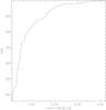 |
Fig. B.1 Evolution of the S/N as a function of CRth. |
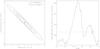 |
Fig. B.2 Left panel: χ2 distribution of the period and period derivative of the magnetar. The contours are the 68%, 90% and 99% of confidence level on the parameters. Right panel: folded light curve on the four XMM-Newton observations with our best fit parameters (see Table B.1). |
We use this folded light curve to compute the count rate threshold which maximizes the
signal-to-noise ratio. As the magnetar flux is an additional noise on the Sgr
A* light curve, magnetar
flux contribution at each phase (τ) of the folded light curve is
 with CRfold the count rate of
the folded light curve and CRSgr A∗ = 0.10 count
s-1 the non-flaring level of Sgr A* seen with pn (e.g., Mossoux et al. 2015a). The signal-to-noise ratio is
with CRfold the count rate of
the folded light curve and CRSgr A∗ = 0.10 count
s-1 the non-flaring level of Sgr A* seen with pn (e.g., Mossoux et al. 2015a). The signal-to-noise ratio is
 (B.2)The phase τ which maximizes the
S/N allows us to compute the corresponding count rate threshold
(CRth). Figure B.1 shows that there is no optimum value of the count
rate threshold maximizing the S/N. Thus, we consider a count rate
threshold which filters out 50% of the magnetar flux. This threshold is 0.27 count s-1 and keeps 50% of
the observation time. Then, from P and Ṗ, the time interval during which the count rate of
the folded light curve is lower than CRth can be computed
for all observations from Eq. (B.1). Thus
we can construct a new GTI file which is the combination of the GTI file from the event
list of pn (which contains the time interval during which the cameras do not observe) and
the GTI file created by removing the magnetar pulse using the SAS task
gtimerge.
(B.2)The phase τ which maximizes the
S/N allows us to compute the corresponding count rate threshold
(CRth). Figure B.1 shows that there is no optimum value of the count
rate threshold maximizing the S/N. Thus, we consider a count rate
threshold which filters out 50% of the magnetar flux. This threshold is 0.27 count s-1 and keeps 50% of
the observation time. Then, from P and Ṗ, the time interval during which the count rate of
the folded light curve is lower than CRth can be computed
for all observations from Eq. (B.1). Thus
we can construct a new GTI file which is the combination of the GTI file from the event
list of pn (which contains the time interval during which the cameras do not observe) and
the GTI file created by removing the magnetar pulse using the SAS task
gtimerge.
Appendix C: The two X-ray flares seen in EPIC/pn, MOS1 and MOS2 cameras
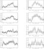 |
Fig. C.1 XMM-Newton light curve of the X-ray from Sgr A* in the 2−10 keV energy range. Left panels: the light curve of flare 1 on 2014 Mar. 10 flare binned on 500 s. Right panels: the light curve of flare 2 on 2014 Apr. 2 flare binned on 100 s. The total (pn+MOS1+MOS2) light curve is shown in the top panel. The light curves of EPIC/pn, MOS1 and MOS2 are shown in the second, third and bottom panels. The crosses are the data points of the total light curve. The horizontal dashed line and the solid line are the sum of the non-flaring level and the smoothed light curve for each instrument. The dashed lines represent the Bayesian blocks. The solid line and the gray curve are the smoothed light curve and the associated errors (h = 500 and 100 s for flare 1 and 2, respectively). The vertical gray stripe is the time during which the camera did not observe. |
Figures C.1 shows the flare light curves obtained with EPIC on board XMM-Newton on 2014 Mar. 10 (left panels) and Apr. 2 (right panels). The Bayesian-blocks algorithm characterizes the 2014 Mar. 10 flare with two blocks in the pn light curve but only with one block in the MOS1 and MOS2 light curves. Moreover, the duration of the flares seen in each camera is different (see Table C.1). This can be explained by the lower number counts in MOS1 and MOS2 because of the RGS: the number of photons recorded by pn during the flare is larger and thus the accuracy on the determination of the beginning and end of the flare is better.
The flare on 2014 Apr. 2 is not detected by the Bayesian-blocks algorithm in MOS1 and MOS2 because the amplitude and the number of counts in this flare is rather small.
Characteristics of the X-ray flare observed by EPIC/MOS on 2014 Mar. 10.
All Tables
Coordinated observation log with SINFONI at ESO’s VLT for the 2014 Feb.–Apr. campaign.
Characteristics of the X-ray flares observed by XMM-Newton in 2014 after removing the magnetar contribution.
All Figures
|
Fig. 1 Time diagram of the 2014 Feb.−Apr. campaign. The horizontal dashed lines are the XMM-Newton orbital visibility times of Sgr A* labeled with revolution numbers. The thick solid lines are the time slot of the observations for each instrument with start and stop hours. The vertical dotted lines are the limits of the XMM-Newton observations. The vertical gray blocks are the X-ray (Arabic numerals) and near-IR (Roman numerals) flares reported in this work. |
| In the text | |
|
Fig. 2 XMM-Newton/EPIC (pn+MOS1+MOS2) light curves of Sgr A* in the 2−10 keV energy range obtained 2014 Feb.−Apr. The time interval used to bin the light curve is 300 s. The X-ray flares are labeled with Arabic numerals. The horizontal lines below these labels indicate the flare durations. |
| In the text | |
|
Fig. 3 XMM-Newton light curve binned on 500 s of the 2014 Mar. 10 flare from Sgr A* in the 2−10 keV energy range. Top panel: the crosses are the data points of the EPIC/pn light curve. The dashed lines represent the Bayesian blocks. The solid line and the gray curve are the smoothed light curve and the associated errors (h = 500 s). Bottom panel: the total (pn+MOS1+MOS2) light curve. The horizontal dashed line and the solid line are the sum of the non-flaring level and the smoothed light curve for each instrument. The vertical gray stripe is the time during which the camera did not observe. |
| In the text | |
|
Fig. 4 XMM-Newton light curve binned on 100 s of the 2014 Apr. 2 flare from Sgr A* in the 2−10 keV energy range. The window width of the smoothed light curve is 100 s. See caption of Fig. 3 for panel description. |
| In the text | |
|
Fig. 5 XMM-Newton/MOS1 (left column) and MOS2
(right column) images of Sgr A* on 2014 Mar. 10. The energy range
is 2–10 keV. The field of view is 20″ ×
20″, the pixel size is |
| In the text | |
|
Fig. 6 Best-fit parameters of the 2014 Mar. 10 (top) and 2014 Apr. 2 (bottom) flares. The diagonal plots are the marginal density distribution of each parameter. The median values of each parameter are represented by the vertical dotted lines in diagonal plots and by a cross in other panels; the vertical dashed lines define the 90% confidence interval (see Table 7 for the exact values). The contours are 68%, 90% and 99% of confidence levels. |
| In the text | |
|
Fig. 7 XMM-Newton/EPIC pn spectrum of the 2014 Mar. 10 (top) and 2014 Apr 2 (bottom) flares. The model is the best spectrum obtained with MCMC (see text for details). The lower panel in the two graphs is the residual. The horizontal and vertical lines are the spectral bins and the error on the data, respectively. |
| In the text | |
|
Fig. 8 Unabsorbed total energy vs. unabsorbed peak luminosity of the X-ray flares (adapted from Mossoux et al. 2015a). The top x-axis is the unabsorbed fluence. The crosses represent the X-ray flares from the Chandra XVP campaign (Neilsen et al. 2013), the triangles are the two brightest flares seen with XMM-Newton (Porquet et al. 2003, 2008), the diamond and the two squares are the 2011 March 30 flare and its subflares, respectively (Mossoux et al. 2015a). The empty circles are X-ray flares 1 and 2 of this work with their 1σ error bars. The filled circles are the components 1a and 1b of flare 1 (see Sect. 4.1.2). |
| In the text | |
|
Fig. 9 Light curves of Sgr A* obtained with WFC3 on board HST during 2014 Feb.−Apr. The NIR flares are labeled with Roman numerals. The horizontal lines below these labels indicate the flare durations. The error bar in each panel is standard deviation of the photometry. |
| In the text | |
|
Fig. 10 Histogram of the NIR flux densities from Sgr A* observed in the Ks-band with NACO at ESO’s VLT (adapted from Fig. 3 of Witzel et al. 2012). Top panel: the solid line is the normalized distribution of the NIR flux densities corrected from the background emission. The dashed lines are the amplitude of the HST flares I, II and the lower limit of the amplitude of the flare III extrapolated to the Ks-band. We also represented the amplitude above the 3σ limit of the VLT flares IV and V extrapolated to the Ks-band. The dot-dashed line is the detection limit corresponding to 3 times the standard deviation of the quiescent flux density of HST on 2014 Mar. 10. Bottom panel: the cumulative distribution function of the NIR flux densities from Sgr A* corrected from the background emission. |
| In the text | |
|
Fig. 11 Light curves of Sgr A* obtained with SINFONI at ESO’s VLT during 2014 Apr. 3 and 4. The dash-dotted lines represent the 3σ detection level of Sgr A*. The horizontal segments indicate the exposure length of 400 s. The NIR flares are labeled with Roman numerals. |
| In the text | |
|
Fig. 12 CARMA light curves at 3.2 mm (95 GHz) of Sgr A* (white circle) and 1733-130 (black circle) in April 2014. The dash-dotted line represents the mean flux density. |
| In the text | |
|
Fig. 13 VLA light curves of Sgr A* obtained on 2014 Mar. 1 (8.56 GHz), Mar. 10 (13.37 GHz) and Apr. 2 (1.68 and 5.19 GHz). The y-axis covers the same range of flux density for all observation and is centered on the mean of the minimum and maximum flux density in each panel. |
| In the text | |
|
Fig. 14 Simultaneous X-ray, NIR and radio observations of flare I/1 from Sgr A* on 2014 Mar. 10. Top panel: the EPIC/pn smoothed light curve computed with a window width of 500 s and its error in gray. The dashed lines are the Bayesian blocks. Middle panel: the deredened HST light curve and its error in gray. The vertical dot-dashed lines are the beginning and the end of the flares. Bottom panel: the VLA light curve at 13.37 GHz. The vertical dot-dashed line is the time of the change of slope. The dashed broken line is the fit. |
| In the text | |
|
Fig. 15 Evolution of the ratio between NIR and X-rays during flare I/1 on 2014 Mar. 10. Top panel: the dashed line surrounded by the dark gray error bars corresponds to the smoothed light curve of the X-ray flare and its flux can be seen on the left y-axis. The solid line and the light gray error bars is the NIR light curve whose flux is read on the right y-axis. Bottom panel: the flux of the X-ray light curve divided by the NIR one. |
| In the text | |
|
Fig. 16 NIR/X-ray peak ratio vs. time delay for the synchrotron-inverse Compton process. The asterisks are the results reported by Yusef-Zadeh et al. (2012), the solid line is a parabolic fit. The horizontal solid line and gray box are the lower limit and error bar on the NIR/X-ray peak ratio of the flare I/1 on 2014 Mar. 10 and the corresponding time-delay range. The dashed line is the ratio between the maximum NIR amplitude reported by Witzel et al. (2012) and the X-ray peak of flare 1, with the gray box being the corresponding error bar (see text for details). |
| In the text | |
|
Fig. 17 Light curve fitting of the HST NIR flares (left panels) and the X-ray (right panels) counterparts. The solid lines are the observed light curves with the error bars in gray. The dashed lines in right panels are the Bayesian blocks. The X-ray light curves are smoothed with a window width of 500 s and 100 s for 2014 Mar. 10 and Apr. 2, respectively. The dotted lines are the individual Gaussians and the dot-dashed line is the sum of the Gaussians. The vertical dotted lines are the time of the NIR flare peak when there is no detected X-ray counterpart. The residuals are in units of σ. |
| In the text | |
|
Fig. 18 NIR-to-X-ray peak ratio vs. amplitude of the NIR flares. Squares refer to the flares reported in Table 3 of Eckart et al. (2012b). Triangles are the simultaneous NIR/X-ray flares detected on 2007 Apr. 4 and labeled D and E in Table 2 of Trap et al. (2011). Diamonds are the delayed flares of 2004 Jul. 7, 2008 Jul. 26+27 and 2008 May 5 reported in Table 2 of Yusef-Zadeh et al. (2012). The labeled points are the NIR and X-ray flares observed during this campaign. |
| In the text | |
|
Fig. 19 Physical parameters of the flares observed simultaneously in X-rays and NIR for the three emission models. The flare Ia/1a, Ib/1b and IIIa/2 are in the upper, middle and bottom panels, respectively. Left panels are the size of the flaring-source region (θ) vs. the peak of the spectrum (Sm) at the frequency νm. Right panels are the density of the relativistic electrons vs. the magnetic field. The locii where the Synchrotron Self-Compton−Synchrotron Self-Compton (SSC-SSC), Synchrotron-Synchrotron Self-Compton (SYN-SSC) and Synchrotron-Synchrotron (SYN-SYN) are dominant are shown in black, blue and green, respectively. The red dots represent the turnover frequencies from 50 to 3000 GHz by step of 200 GHz. The arrows show the direction of the curves if the limit on the alternative emission processes is lowered. Dotted lines are locii of SYN-SSC where the MIR emission is larger than the observed upper-limit values (see text for details). |
| In the text | |
|
Fig. 20 Physical parameters of the flares only observed in NIR for the three emission models. The NIR flare II, IIIb, IV and V are in the upper, second, third and bottom panels, respectively. See Fig. 19 caption for the panel description. |
| In the text | |
|
Fig. A.1 Comparison of the flare detection level with the non-flaring level corresponding to those of the 2011 (left panel) and February 2014 (right panel) observations. The vertical doted-dashed line represents an example flare with the same amplitude above the non-flaring level for a 2011 and 2014 Feb.−Apr. observations. |
| In the text | |
|
Fig. A.2 Flare distribution seen by Chandra and the detection probability of the Bayesian-blocks algorithm during an observation with XMM-Newton. The crosses are the X-ray flares detected during the Chandra XVP campaign of 2012. Left panel: the flare amplitude above the non-flaring level seen by EPIC/pn during the 2011 campaign. Right panel: the flare amplitude above the non-flaring level seen by EPIC/pn during the 2014 Feb. 28 observation. |
| In the text | |
|
Fig. B.1 Evolution of the S/N as a function of CRth. |
| In the text | |
|
Fig. B.2 Left panel: χ2 distribution of the period and period derivative of the magnetar. The contours are the 68%, 90% and 99% of confidence level on the parameters. Right panel: folded light curve on the four XMM-Newton observations with our best fit parameters (see Table B.1). |
| In the text | |
|
Fig. C.1 XMM-Newton light curve of the X-ray from Sgr A* in the 2−10 keV energy range. Left panels: the light curve of flare 1 on 2014 Mar. 10 flare binned on 500 s. Right panels: the light curve of flare 2 on 2014 Apr. 2 flare binned on 100 s. The total (pn+MOS1+MOS2) light curve is shown in the top panel. The light curves of EPIC/pn, MOS1 and MOS2 are shown in the second, third and bottom panels. The crosses are the data points of the total light curve. The horizontal dashed line and the solid line are the sum of the non-flaring level and the smoothed light curve for each instrument. The dashed lines represent the Bayesian blocks. The solid line and the gray curve are the smoothed light curve and the associated errors (h = 500 and 100 s for flare 1 and 2, respectively). The vertical gray stripe is the time during which the camera did not observe. |
| In the text | |
Current usage metrics show cumulative count of Article Views (full-text article views including HTML views, PDF and ePub downloads, according to the available data) and Abstracts Views on Vision4Press platform.
Data correspond to usage on the plateform after 2015. The current usage metrics is available 48-96 hours after online publication and is updated daily on week days.
Initial download of the metrics may take a while.