| Issue |
A&A
Volume 573, January 2015
|
|
|---|---|---|
| Article Number | A106 | |
| Number of page(s) | 27 | |
| Section | Interstellar and circumstellar matter | |
| DOI | https://doi.org/10.1051/0004-6361/201424979 | |
| Published online | 06 January 2015 | |
The dense gas mass fraction in the W51 cloud and its protoclusters⋆,⋆⋆
1 European Southern Observatory, Karl-Schwarzschild-Strasse 2, 85748 Garching bei München, Germany
e-mail: Adam.G.Ginsburg@gmail.com
2 CASA, University of Colorado, 389-UCB, Boulder, CO 80309, USA
3 Harvard-Smithsonian Center for Astrophysics, 60 Garden Street, Cambridge, MA 02138, USA
4 University of Alberta, Department of Physics, 4-181 CCIS, Edmonton AB T6G 2E1, Canada
5 Department of Astronomy, Yale University, PO Box 208101, New Haven, CT 06520-8101, USA
6 Department of Physical Sciences, University of Puerto Rico, PO Box 23323, San Juan, PR 00931, USA
Received: 12 September 2014
Accepted: 29 October 2014
Context. The density structure of molecular clouds determines how they will evolve.
Aims. We map the velocity-resolved density structure of the most vigorously star-forming molecular cloud in the Galactic disk, the W51 giant molecular cloud.
Methods. We present new 2 cm and 6 cm maps of H2CO, radio recombination lines, and the radio continuum in the W51 star forming complex acquired with Arecibo and the Green Bank Telescope at ~ 50″ resolution. We use H2CO absorption to determine the relative line-of-sight positions of molecular and ionized gas. We measure gas densities using the H2CO densitometer, including continuous measurements of the dense gas mass fraction (DGMF) over the range 104cm-3<n(H2) < 106cm-3 – this is the first time a dense gas mass fraction has been measured over a range of densities with a single data set.
Results. The DGMF in W51 A is high, f ≳ 70% above n> 104cm-3, while it is low, f< 20%, in W51 B. We did not detect any H2CO emission throughout the W51 GMC; all gas dense enough to emit under normal conditions is in front of bright continuum sources and therefore is seen in absorption instead.
Conclusions. (1) The dense gas fraction in the W51 A and B clouds shows that W51 A will continue to form stars vigorously, while star formation has mostly ended in W51 B. The lack of dense, star-forming gas around W51 C indicates that collect-and-collapse is not acting or is inefficient in W51. (2) Ongoing high-mass star formation is correlated with n ≳ 1 × 105cm-3 gas. Gas with n> 104cm-3 is weakly correlated with low and moderate mass star formation, but does not strongly correlate with high-mass star formation. (3) The nondetection of H2CO emission implies that the emission detected in other galaxies, e.g. Arp 220, comes from high-density gas that is not directly affiliated with already-formed massive stars. Either the non-star-forming ISM of these galaxies is very dense, implying the star formation density threshold is higher, or H ii regions have their emission suppressed.
Key words: turbulence / ISM: clouds / HII regions / ISM: molecules / ISM: structure / radio lines: ISM
The data set has been made public at http://dx.doi.org/10.7910/DVN/26818
Appendices are available in electronic form at http://www.aanda.org
© ESO, 2015
1. Introduction
Massive star clusters, those containing > 104M⊙ of stars, are among the most visually outstanding features in the night sky (see review by Longmore et al. 2014). In other galaxies, they are useful probes of the star formation history and can be individually identified and measured (Bastian 2008). Locally, they are the essential laboratories in which we can study the formation of massive stars (Davies 2012).
In order to utilize these clusters as laboratories, we need to understand their formation in detail. Clusters are often assumed and measured to be coeval to within a narrow range (e.g. 105 yr; Kudryavtseva et al. 2012), but uncertainties remain (Beccari et al. 2010). In the most massive clusters, there are predictions that multiple generations or an extended generation of stars should form prior to gas expulsion because the gas will remain gravitationally bound (Bressert et al. 2012). Feedback from and within young massive clusters is an active field of numerical study (Rogers & Pittard 2013; Dale et al. 2005, 2013, 2012; Dale & Bonnell 2008; Parker & Dale 2013; Myers et al. 2014; Krumholz et al. 2014). While only 5−35% of all stars form in bound clusters1 (Kruijssen 2012), these clusters form the basis of our understanding of stars and stellar evolution (Kalirai & Richer 2010), and understanding their formation is therefore crucial.
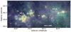 |
Fig. 1 A color composite of the W51 region with major regions, W51 A, B, and C, labeled. W51 A contains the protoclusters W51 Main and W51 IRS 2; these are blended in the light orange region around 49.5−0.38. The blue, green, and red colors are WISE bands 1, 3, and 4 (3.4, 12, and 22 μm) respectively. The yellow-orange semitransparent layer is from the Bolocam 1.1 mm Galactic Plane Survey data (Aguirre et al. 2011; this paper). Finally, the faint whitish haze filling in most of the image is from a 90 cm VLA image by Brogan et al. (2013), which primarily traces the W51 C supernova remnant. This haze is more easily seen in Fig. B.6. |
The results of cluster formation may be decided before the first stars are formed. The starless initial conditions of massive clusters have not yet been definitively observed (Ginsburg et al. 2012) though there are viable candidates such as G0.253+0.016 (Longmore et al. 2012). The initial conditions for star formation on any scale are clearly turbulent. However, there is no evidence whether these initial conditions differ in any qualitative way from turbulence in local, low-mass star-forming regions.
Star formation appears to occur efficiently only above a volume density threshold in molecular gas, specifically n(H2) ≳ 104cm-3, in the Galactic disk (Lada et al. 2010, who advocate a column density threshold corresponding to this density); note however that the threshold is smooth, not a step function as implied by the term (Padoan et al. 2014). The dense gas mass fraction has been measured for various definitions of dense (Battisti & Heyer 2014; Wu et al. 2005), but these definitions don’t always correspond to the associated threshold (Kauffmann & Pillai 2010; Parmentier et al. 2011; Parmentier 2011). Often, the dense gas threshold is observationally defined as the threshold to see a given molecule, which is sometimes incorrectly assumed to correspond to a fixed critical density for the molecule. The existence of a universal density threshold for star formation is contentious (Burkert & Hartmann 2013; Clark & Glover 2013); the star formation threshold likely varies with the turbulent properties of clouds (Longmore et al. 2013; Kruijssen 2014; Hennebelle & Chabrier 2011, 2013; Padoan & Nordlund 2011; Krumholz et al. 2005). Star formation thresholds can only be evaluated when measurements of density and column density are simultaneously available.
1.1. W51
The W51 cloud complex (Fig. 1), containing the two massive protocluster candidates W51 Main and W51 IRS 2 from Ginsburg et al. (2012), is located at ℓ ~ 49,b ~ − 0.3, very near the Galactic midplane2 at a distance of 5.1 kpc (Sato et al. 2010). It is a well-known and thoroughly studied collection of clouds massing M> 106M⊙ (Carpenter & Sanders 1998; Bieging et al. 2010; Kang et al. 2010; Parsons et al. 2012). The radio-bright regions are generally known as W51 A to the east, W51 B to the west, and W51 C for the southern component, known to trace a supernova remnant (Koo et al. 1995; Brogan et al. 2000, 2013).
1.2. Formaldehyde
Formaldehyde (H2CO) has been recognized as a useful probe of physical conditions in the molecular interstellar medium for decades (Mangum & Wootten 1993). The centimeter lines, H2CO110 − 111 (6.2 cm, 4.82966 GHz) and 211 − 212 (2.1 cm, 14.48848 GHz), have a peculiar excitation process in which collisions overpopulate the lower of the two Kc rotational states, where Kc is the quantum number representing the angular momentum projected onto the long axis of the molecule. The overpopulated lower-energy state leads to amplified absorption, or effective excitation temperatures less than the background temperature, allowing H2CO centimeter absorption to be seen against the cosmic microwave background (CMB). Because the 110 − 111 and 211 − 212 level pairs populate differently depending on the volume density of the colliding partner (a mix of p-H2, He, and o-H2), their ratio is sensitive to the local gas volume density3.
H2CO110 − 111 has been observed in the W51 Main region with the VLA (Martin-Pintado et al. 1985a) and Westerbork (Arnal & Goss 1985), and this data was used to gain some early constraints on the geometry of the region (e.g. Carpenter & Sanders 1998). Henkel et al. (1980) presented observations of the 110 − 111 and 211 − 212 lines, and Martin-Pintado et al. (1985b) presented single-dish mapping observations of the H2CO211 − 212 line toward the W51 Main region, but both treated the region as a single-density structure.
1.3. Paper overview
We present a detailed examination of the dense gas in the W51 cloud complex. Section 2 presents the observations and data reduction. Section 3 describes the analysis techniques, including measurement of the dense gas mass fraction and derivation of the cloud geometry. Section 4 discusses the implications of the density measurements for Galactic clouds and extragalactic interstellar media. Section 5 concludes. There are two appendices: Appendix A describes the radio recombination line and continuum data. Appendix B describes details of individual regions, with a focus on the cloud and H ii region line-of-sight geometry.
2. Observations and data reduction
The W51 survey was performed in September 2011 on the Green Bank Telescope (GBT) and in 2012 using the Arecibo Observatory. The data was reduced using custom-made scripts based off of both GBTIDL’s mapping routines by Glen Langston4 and Phil Perillat’s AOIDL routines. The code is available at https://github.com/keflavich/sdpy. The data reduction code and workflow are included in a corresponding git repository5.
2.1. Arecibo 6 cm
The Arecibo data were taken as part of project A2705 over the course of 4 nights, September 10, 11, 12, and 15 2012. The Mock spectrometer was used to cover the range 4.6 to 5.4 GHz with a spectral resolution ~1 km s-1, including the o - H2CO 4.82966 GHz line and the H107-H112α recombination lines. On the first night, September 10 2012, a significant fraction of the data was lost due to an internal instrument error within the Mock spectrometer, which resulted in a loss of the high spectral resolution component of the H2CO data for that night. As a result, we have focused our study on the lower-resolution (~ 1 km s-1) data.
The fields were observed with east-west maps using the C-band receiver. No crosshatching was performed with Arecibo.
The Arecibo data reduction process for W51 presented unique challenges: at C-band, the entire region surveyed contains continuum emission, so no truly suitable off position was found within the survey data. Similarly, H2CO is ubiquitous across the region, so it was necessary to mask out the absorption lines when building an off position. This was done by interpolating across the line-containing region of the spectrum with a polynomial fit. The fits were inspected interactively and tuned to avoid over-predicting the background.
The Arecibo data were corrected to main beam brightness temperature TMB using a main-beam efficiency as a function of zenith angle in degrees (za):
 This is a fit to 5 years worth of calibration data acquired at Arecibo and assembled by Phil Perrilat6.
The maps were made by computing an output grid in Galactic coordinates with 15′′ pixels and adding each spectrum to the appropriate pixel7. In order to avoid empty pixels and maximize the signal-to-noise (S/N), the spectra were added to the grid with a weight set from a Gaussian with FWHM = 20″, which effectively smooths the output images from FWHM ≈ 50″ to ≈54″. See Mangum et al. (2007) for more detail on the on-the-fly mapping technique used here.
The Arecibo data were taken at a spectral resolution of 0.68 km s-1. The spectra were regridded onto a velocity grid from − 50 to 150 km s-1 with 1 km s-1 resolution. To achieve this, they were first Gaussian-smoothed to FWHM = 1 km s-1 then downsampled appropriately.
The position-position-velocity (PPV) cubes were created with units of brightness temperature. The Arecibo cubes have contributions from 15−20 independent spectra in each pixel, though this hit rate varies in a systematic striped pattern parallel to the Galactic plane. The small overlap regions between different maps have a significantly higher number of samples; these regions constitute a small portion of the map. The resulting noise level is rms ~ 50 − 60 mK except toward the H ii regions, where it peaks at about 400 mK. The continuum is derived by averaging line-free channels; its S/N peaks at ~ 900.
The Arecibo data have smaller systematic continuum offsets than the GBT data (Fig. 2), but they are more visually pronounced because there is much more diffuse emission at 6 cm. The continuum zero-point level in the Arecibo data was set to be the 10th percentile value of each scan, which is effectively the minimum value across each scan but with added robustness against noise-generated false minima. In the eastmost and westmost blocks, this strategy was very effective, as there are clearly areas in each scan that see no continuum. However, in the central block, this approach resulted in a vertical negative filament that almost certainly represents a local minimum that should be positive. This negative filament has values ≳− 0.08 K. Given the excellent agreement between the three independently observed regions in the areas that they overlap, it is clear that the continuum is reliable above ≳0.5 K, which is the entire regime in which it is a significant contributor to the total background emission (at lower levels, the CMB is dominant).
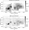 |
Fig. 2 Continuum images of (a) the 6 cm Arecibo data and (b) 2 cm GBT data. |
2.2. GBT 2 cm
The GBT data were taken as part of program AGBT10B/019. We used the GBT Spectrometer with 4 windows covering the o - H2CO 14.488479 GHz line, H77α (14.12861 GHz), and two others that were not reduced targeting H2CN (14.82579 GHz) and NaCl and SO (13.03606 GHz); online examination of the latter windows suggested that we did not detect any emission or absorption. The data presented in this paper include sessions 10, 11, 14, 16, 17, 20, 21, and 22; the other sessions from this project include maps of outer galaxy regions and a single-pointing survey of Galactic plane sources that will be presented in another paper.
Data were taken in on-the-fly mode with the GBT Ku-band dual-beam system. Cross-hatched north-south and east-west maps were created in Galactic coordinates. Each spectrum was calibrated using the first and last scans of each observation as off positions. The background level to be subtracted off of the continuum was determined by linearly interpolating between these scans.
The Green Bank data have a main beam efficiency ηMB = 0.886, or a gain of 1.98 K/Jy assuming a 51′′ beam (see Mangum et al. 2013, for additional discussion). The GBT data were also corrected for atmospheric opacity using Ron Maddalena’s getForecastValues8 with a typical zenith optical depth τz ≈ 0.02; this correction was never more than ~5%. The GBT data were taken with a spectral resolution Δv = 0.25 km s-1
Typical noise levels were ~10−20 mK per 1 km s-1 channel; the levels vary across the map.
The GBT data were mapped in an orthogonal grid pattern, so the hit coverage is more uniform on small scales than the Arecibo data, but because of the dual-beam Ku-band system, the overall noise levels are much more patchy. Additionally, the nights with better weather yielded a lower noise level. The noise ranges from ~7 mK in the W51 Main region to ~20 mK in the westmost region. As with the Arecibo data, the H ii region adds noise, but the peak noise towards an H ii region is only ~20 mK. This difference is because the diffuse H ii region is fainter at 2 cm. The S/N in the continuum peaks at ~400.
While the noise in the continuum is nominally quite low, there are significant systematic effects visible in the continuum maps. The continuum zero-point of each GBT map was determined by assuming that the first and last scan both observed zero continuum and that the sky background can be linearly interpolated between the start and end of the observations. In general, these are good assumptions, but they leave in systematic offsets of up to ≲− 0.15 K in the maps, most likely because there is a ~ 0.15 K variation in the diffuse background emission.
2.3. Optical depth data cubes
The data cubes were converted into optical depth data cubes by dividing the integrated H2CO absorption signature by the measured continuum level. We added a fixed background of 2.73 K to the reduced images to account for the CMB, which is absent from the images due to the background-subtraction process. We define an observer’s optical depth
![\begin{equation} \tau_{\rm obs} = -\ln\left[\frac{T_{\rm MB}}{T_{\rm bg}}\right] \end{equation}](/articles/aa/full_html/2015/01/aa24979-14/aa24979-14-eq46.png) (1)as opposed to the true optical depth, which is modeled in radiative transfer calculations
(1)as opposed to the true optical depth, which is modeled in radiative transfer calculations ![\begin{equation} \tau = -\ln\left[\frac{T_{\rm MB}-T_{\rm ex}}{T_{\rm bg}-T_{\rm ex}}\right]\cdot \end{equation}](/articles/aa/full_html/2015/01/aa24979-14/aa24979-14-eq47.png) (2)The approximation τobs = τ is valid for Tex ≪ Tbg, which is true when an H ii region is the backlight but generally not when the CMB is. Displaying the data on this scale makes regions of similar gas surface density appear the same, rather than being enhanced where there are backlights. The noise is correspondingly suppressed where backlighting sources are present.
(2)The approximation τobs = τ is valid for Tex ≪ Tbg, which is true when an H ii region is the backlight but generally not when the CMB is. Displaying the data on this scale makes regions of similar gas surface density appear the same, rather than being enhanced where there are backlights. The noise is correspondingly suppressed where backlighting sources are present.
H2CO absorption is ubiquitous across the map. In the Arecibo data, 8044 of 17 800 spatial pixels have peak optical depths >5σ, and 14 547 have peaks >3σ, so H2CO absorption is detected at ~ 80% of the observed positions.
The GBT H2CO211 − 212 data have lower peak signal-to-noise because the continuum background is lower. Additionally, the 211 − 212 line is expected to trace denser gas and therefore be detected along fewer lines of sight. The 211 − 212 line is detected with a peak at >5σ in 3497 pixels (20%) and > 3σ in 12 254 pixels (69%). The high detection rate validates H2CO as an efficient dense-gas tracer.
There were no detections of H2CO110 − 111 or 211 − 212 emission. The significance of the nondetection of emission is discussed in Sect. 4.3.
2.4. A note on nondetections
H213CO was not detected anywhere in the W51 complex in either the 110 − 111 or 211 − 212 lines. The peak signal-to-noise in the H2CO110 − 111 cube was 180 at 1 km s-1 resolution (corresponding to an optical depth τobs ~ 1/5 at the peak continuum detection point), so we report a 3σ upper limit on the H2CO/H213CO ratio R> 60, which is consistent with solar values of the 12C/13C ratio.
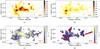 |
Fig. 3 Peak observed optical depth τobs = −ln(TMB/Tcontinuum) in the a) 110 − 111 and b) 211 − 212 lines and c) their ratio, 110 − 111/211 − 212. Figure d) shows the true optical depth ratio assuming Tex(110 − 111) = 1.0 K and Tex(211 − 212) = 1.5 K; these are reasonable and representative excitation temperatures but they are not fits to the data. The data are masked with a filter described in Sect. 3.2 and cover the range 75 >VLSR> 40 km s-1; see Figs. 4 and 5 for individual velocity components. In general, lower (redder) ratios in Figs. c) and d) indicate higher densities, however in the filament at 49.0−0.3, the low ratio is due to the geometry in which Tcontinuum is in the foreground of the molecular gas. |
3. Analysis
3.1. H2CO modeling
The H2CO line ratio can be transformed into a volume density of hydrogen n(H2) using large velocity gradient model grids. The column density of o - H2CO, the ortho-to-para-ratio of H2, and the gas temperature are the three main nuisance parameters that can be marginalized over.
The o - H2CO column density is degenerate with the velocity gradient in LVG models. The H2 column density is degenerate with this gradient and the abundance of o - H2CO. Precise measurements of the H2CO abundance are not generally available, but typical values of Xo - H2CO = 10-10 − 10-8 relative to H2 are generally assumed (Mangum & Wootten 1993; Ginsburg et al. 2011; this paper; Ao et al. 2013) and found to be consistent with the observations. Nonetheless, little is known about local variations in o - H2CO abundance, except that it freezes out in cold, dense cores (Young et al. 2004). The abundance was left as a free parameter in the model fitting.
The model grids were generated using RADEX LVG models (python wrapper9; original code van der Tak et al. 2007) and the grids were fit using https://github.com/keflavich/h2co_modeling. The RADEX models assume a velocity gradient of 1 km s-1pc-1. Ginsburg et al. (2011, this paper) discussed the effect of a local gas density distribution on the molecular excitation, but due to the complexity involved in accounting for these effects, we ignore them here. The derived physical parameters are moderately sensitive to the input collision rates, with a 50% error in collision rates yielding a factor of 2 error in derived density (Zeiger & Darling 2010), but the error on the collision rates in the low temperature regime we are modeling have recently been improved from the previously used Green (1991) rates and should not be a dominant factor in our calculations (Troscompt et al. 2009; Wiesenfeld & Faure 2013).
3.2. H2CO observables
Figure 3 shows the most important observed properties of the H2CO lines. The figures show the peak observed optical depth τobs = −ln(TMB/Tcontinuum) in each line along with the ratio of the 110 − 111 to the 211 − 212 optical depth. The noise is computed by measuring the standard deviation over a signal free region (− 50 to 0 km s-1) along each spatial pixel. The cubes were masked to show significant pixels determined by:
-
1.
Selecting all voxels withS/N> 2 in both images or S/N> 4 in either and with at least 7 (of 26 possible) neighbors also having S/N> 2
-
2.
Selecting all voxels with ≥10 neighbors having S/N> 2
-
Growing (dilating) the included mask region by 1 pixel in all directions
-
4.
Selecting all voxels with ≥5 neighbors marked as included by the above steps (this is a closing operation)
-
5.
(2D only) When used to mask 2D images, the selection mask is then collapsed along the spectral axis such that any pixel containing at least one voxel along the spectral axis is included.
This approach effectively includes all significant pixels and all reliably detected regions within the data cube, though the number of neighbors used at each step and the selected growth size are somewhat arbitrary and could be modified with little effect.
Figures 3−5 each contain peak optical depth maps and two ratio maps. The first ratio map shows the observed optical depth ratio, while the second shows the true optical depth ratio assuming an excitation temperature for each line, Tex(110 − 111) = 1.0 K and Tex(211 − 212) = 1.5 K. These excitation temperatures are representative of those expected for most of the modeled parameter space in which absorption is expected. Fitting of individual lines-of-sight confirm that good fits can be achieved using these assumed temperatures.
However, there are some clear outliers within the map: the clouds at G48.9-0.3 and G49.4-0.2 both show very low 110 − 111/211 − 212 ratios over a broad area. As discussed in Sects. B.2 and B.8, these two regions have H ii regions in the foreground of the molecular gas. The ratios displayed in Fig. 3 are therefore computed with an incorrect background assumed; we correct for the different background in the next section.
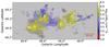 |
Fig. 6 Map of the column-weighted volume density along the line of sight averaged over all velocities. The colors are greyed out where the S/N in the 110 − 111 line is less than ~ 7, with lower-signal regions being progressively more gray. |
3.3. Density maps
We computed the density in each voxel using the χ2 minimization technique from Ginsburg et al. (2011). We measure χ2 over the full 4D parameter space (density, column density, gas temperature, and ortho-to-para ratio [OPR])  (3)The modeled brightness temperature Tmodel is different for each spatial pixel in order to account for the varying continuum background, although for some pixels with significant continuum detected, we still use the CMB as the background continuum because the molecular gas is behind the other continuum emission; see Sect. 3.4.
We have not enforced any constraints on the column density, temperature, or ortho-to-para ratio when fitting. The best-fit value of each of these parameters is taken to be the mean of those parameters over the range  , where
  is the minimum χ2 value.
The gas temperatures returned from the fitting process are, as expected, purely noise: the H2CO110 − 111/211 − 212 ratio provides virtually no constraint on the gas temperature and therefore leaving it as a free parameter has no effect on the fitted density. Similarly, the ortho-to-para ratio of H2 is unconstrained in our data. In principle, the H2 OPR has some effect on H2CO excitation (Troscompt et al. 2009), but in the regime we have modeled and observed, no effect is apparent.
The o - H2CO-column-weighted volume-density along each line of sight is shown in Figs. 6 and 7. The former shows the weighted density over all voxels and the latter shows the weighted density over the two velocity ranges previously discussed. These projections include no information about the errors in the individual fits, which are available from Eq. (3), but by weighting by column density, we have effectively selected the highest S/N points; the statistical errors are therefore negligible relative to the systematic (i.e., those caused by invalid assumptions about the single-zone nature of the models) in these maps. The maps are shown split into two velocity components, v< 62 km s-1 and v> 62 km s-1, which approximately separates out the 68 km s-1 cloud from other components, though because the lines are quite broad the separation is imperfect. Figures B.3 and B.4 show the velocity separation in more detail.
The overall picture is of a central protocluster region (W51 Main and IRS2) with most of the gas mass at a density n ~ 105.5cm-3 within a diameter of ~ 3 pc, surrounded by a rich cloud in which most of the mass is at a density ~ 104cm-3 out to a diameter d ~ 14 pc.
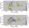 |
Fig. 7 Map of the column-weighted volume density along the line of sight, split into a) the 40−62 km s-1 component and b) the 62 to 75 km s-1 component. The similarity between the two figures is due to large line widths; the cut at 62 km s-1 is meant to highlight the low-density filament around ℓ = 49 and the clouds surrounding W51 Main. |
3.4. Model fitting and geometry
Both H2CO lines are seen only in absorption. However, in some cases the absorption is against a continuum background, while in others the absorption may be only against the CMB.
We have fit the H2CO lines constrained by the LVG models (Sect. 3.1) to spectra averaged over apertures with coherent molecular absorption signatures (e.g., Fig. 8). We compared the χ2 values for fits with the observed continuum as the background to those with the background fixed to TBG = TCMB. We then selected the better of the two fits as representative of the physical conditions. Figures 9 and 10 show the qualitative version of this analysis, highlighting CO-bright regions that lack the expected H2CO absorption signatures and therefore have a different geometry. Regions with the continuum emission in front of the molecular absorption were converted into masks that were then used to decide which models to use for the per-pixel fitting process described in the previous section. The geometric analysis of each region is discussed in detail in Appendix B.
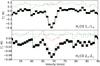 |
Fig. 8 An example of the difference in models between a continuum source (red) and the CMB (green) as the background. The top plot shows the 110 − 111 line and the bottom shows the 211 − 212 line both with the continuum level set to zero in the plot. The residuals are shown offset above the spectra, with the dashed line indicating the zero-residual level. The grey shaded regions show the 1σ error bars on each pixel. The model with the CMB as the only background is able to reproduce the absorption line, while the model with the H ii region in the background cannot account for the depth of the 211 − 212 line. The reduced χ2/n for the models are 14.1 (red) and 2.8 (green), evaluated only over the pixels where the model is greater than the local rms. |
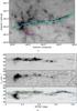 |
Fig. 9 Top figure: a column density map fitted from the Herschel Hi-Gal data with two filament extraction regions superposed in cyan and purple. The purple extracted position-velocity diagram is shown in Fig. 10. Bottom figure: a position-velocity slice of the 68 km s-1 cloud, shown in cyan in the left figure, which includes an 8 μm-dark cloud and the interaction region with the W51C supernova remnant. (bottom figure, top panel) H2CO110 − 111 observed optical depth (bottom figure, middle panel) H2CO211 − 212 observed optical depth (bottom figure, bottom panel) 13CO 1−0 emission from the Galactic Ring Survey (GRS Jackson et al. 2006) with H2CO110 − 111 contours superposed. The weakness of the H2CO absorption on the right half of the cloud corroborates the geometry inferred from comparison of the 110 − 111 and 211 − 212 lines in Fig. 8. The 13CO emission without corresponding H2CO absorption at offset 0.2 degrees is primarily background material in the 51 km s-1 cloud (see Fig. 11. These figures were made using wcsaxes12 and pvextractor13). |
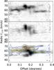 |
Fig. 10 Position-velocity diagrams of filamentary structures to the north and south of W51 Main. The panels are H2CO110 − 111, 211 − 212, and 13CO 1−0 as in Fig. 9. The 50 km s-1 component at offset ~ 0.15 degrees (ℓ ≈ 49.47,b ≈ − 0.42) is in the background of the H ii region. The extracted region is identified in purple in Fig. 9; the left side of the position-velocity diagram corresponds to the b = −0.5 end of the region. |
It is possible that there are multiple continuum emitters along the line of sight in many cases, with the absorbing molecular gas somewhere in the middle. While this possibility adds uncertainty to the measurements, there are some cases in which the dominant continuum can unambiguously be assigned a foreground or background position.
Summary figures of our geometric analysis are shown in the cartoon Fig. 11, with an accompanying labeled on-sky map in Fig. 12.
3.5. Dense gas mass fractions
Because the H2CO densitometer yields a mass-weighted10 measurement of the gas volume density, it is difficult to connect directly to the total gas mass, which is the quantity of interest when determining bulk properties like star forming efficiency. However, because the H2CO and CO chemically trace the same gas, the H2CO-derived density can be applied to the total mass measured by CO. We use the the FCRAO Galactic Ring Survey of 13CO (Jackson et al. 2006) and assume that each 13CO PPV voxel has a mass proportional to its integrated intensity and a density given by the n(H2) delivered from the H2CO densitometer.
The dense gas mass fraction (DGMF) is an oft-quoted measurement used to argue about the speed of the star formation process, the existence of density thresholds, and turbulent properties of the ISM (e.g. Fig. 5 of Krumholz et al. 2007; Battisti & Heyer 2014; Kainulainen et al. 2013; Juneau et al. 2009; Muraoka et al. 2009; Hopkins et al. 2013). However, these fractions are most often quoted as mass of gas at a single density divided by the total mass. We present an improvement on these measurements, showing the continuous distribution of the dense gas mass fraction.
Figure 13 shows the result of using our H2CO PPV density cubes to measure the DGMF from 13CO. We use a range of density thresholds from ~ 103 to ~ 106cm-3. At each density, we identify all voxels in the 13CO PPV cube above that density and integrate those. We then divide by the total integrated 13CO brightness to get the mass fraction: 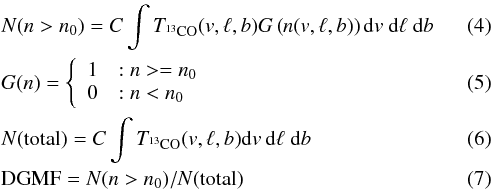 where N is the column of H2 and C = 8.1 × 1020 cm-2/ (K km s-1) is a constant used to convert 13CO brightness to H2 column; it cancels in the DGMF equation.
Figure 14 shows the same results, but for two individual regions: the W51 Main/IRS2 protoclusters and the W51 B region. Within about 10 pc of W51 Main, around half of the mass is at density n> 104cm-3. By contrast, the rest of the molecular cloud shows a consistent fraction f(n> 104 cm-3) ~ 10%.
These DGMF plots are similar to cumulative distribution functions of the column density (e.g. Battersby et al. 2014, Fig. 6), but with the added advantage of assigning a density to each resolution element in both velocity and position.
The multi-density DGMF presented here can be compared to models of global collapse in which progressively more gas should be observed in denser structures over time. They are effectively a gas density cumulative distribution function. However, to understand the systematic effects of line-of-sight stacking of different velocity components (and corresponding radiative transfer issues), similar analysis should be performed on hydrodynamic simulations.
3.5.1. Dense gas fraction assumptions and caveats
The DGMF analysis relies on the 13CO being optically thin and thermally excited, both of which are generally good assumptions for the majority of the mass. The molecular cloud probably includes no more than ~ 20% of its mass in 12CO-dark gas (Pineda & Teixeira 2013; Langer et al. 2014; Smith et al. 2014), which adds little to the overall uncertainty. Similarly, we expect that there is little 13CO-dark molecular gas (the ratio of 12CO to 13CO should not vary significantly in molecular clouds; Visser et al. 2009).
In Sect. 3.3, we discussed the various caveats and issues related to H2CO density fitting. To account for the full range of errors in that analysis, we have plotted the DGMF calculated using the minimum and maximum values of the H2CO-derived density consistent with the data at the 1σ level in Figs. 13 and 14.
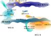 |
Fig. 11 A sketched diagram of the W51 region as viewed from the Galactic north pole, with the observer looking up the page from the bottom (i.e., W51C is the front-most labeled object along our line-of-sight). There are a few significant differences between this and Fig. 29 of Kang et al. (2010), particularly the relative geometry of the cloud and the H ii regions in W51 B. We also show a good deal more detail, revealing that there are H ii regions on both front and back of many clouds. The orange areas represent H ii regions and ionized gas (the W51 C SNR), while purple/blue/cyan regions show molecular clouds. The shapes of the clouds approximately reflect their shape on the sky, but these shapes are only intended as mnemonics to help associate this face-on view with the edge-on view of the real observations. Figure 12 shows the face-on view and can be compared side-by-side with this figure to get an approximate 3D view of the region. |
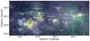 |
Fig. 12 Labeled figures of the W51A and W51B regions, highlighting H ii regions and 8 μm-dark clouds. The colors are described in Fig. 1. These labels can be compared to Fig. 11 to associate labeled regions in the plane of the sky with their counterparts in the face-on view of our Galaxy. |
We have assigned all of the mass associated with a given PPV voxel with a single, fixed density in this analysis. There is certainly some mass at a lower density in each PPV pixel associated with each voxel along that line of sight. This additional mass biases the measured DGMF upwards, but probably only by a small amount at each threshold. This systematic bias can be better characterized by performing a similar analysis on molecular cloud simulations projected into PPV space (as demonstrated for other analysis techniques by Beaumont et al. 2013).
4. Discussion
The W51 cloud complex includes a full range of star forming conditions. In the west, W51 B, there is an older generation of stars including at least one supernova remnant. In the east, there is a pair of forming, still-embedded massive clusters. We have described the geometry of these regions and features of the cloud structures, now we speculate on the broader implications of these observations.
The gas in the W51 B region, while clearly impacted by the expanding W51 C supernova, is less dense than most of the gas in the W51 A region. The supernova feedback is, if anything, destructive; a collect-and-collapse scenario does not fit the observed gas structure since there is less dense gas in the vicinity of the SNR. Given the large radius of the W51 C SNR, ≳100 pc, collection and the early stages of collapse should have happened by now if they are to happen at all.
The proximity of the 68 km s-1 filamentary high velocity stream and the W51 Main protocluster and their relative line-of-sight positions have been presented as evidence for a cloud-cloud collision (Kang et al. 2010). Examination of the H2CO line ratios has shown that the protocluster is embedded in the ~55 km s-1 molecular cloud (e.g. Fig. 10). The velocity difference and their relative positions along the line of sight unambiguously indicate that these components are approaching each other, which is consistent with the cloud-cloud collision hypothesis, though the distinction of these velocity components as individual clouds is somewhat arbitrary since they are components of the same hierarchical medium.
It is possible that the 68 km s-1 cloud is streaming in to a spiral arm, while the 50 km s-1 cloud is slowed down as it exits the spiral arm on the far side. In this scenario, W51 Main is in the deepest part of the spiral arm potential. Gas is accumulating at W51 Main, becoming compressed and undergoing a mini-starburst. The W51 B/C region, with its mature HII regions and SNR, represents a slightly older generation than W51 Main.
The line-of-sight length of the W51 complex is still uncertain, despite our constraints on the relative geometry of different regions. The best prospect for resolving the line-of-sight structure of the region is via precise constraints on distances to the individual regions. Spectrophotometric surveys of the individual stellar sub-clusters may be able to provide this and should be undertaken. Maser parallax observations of different zones may also provide differential distance estimates.
4.1. Gas density and its relation to star formation
To assess the relation between gas density and star formation rate or efficiency, one can multiply the DGMF by the total mass to get a naïve measurement of the total mass directly involved in star formation (Fig. 15 transformed to Fig. 16). We have compared this map to the distribution of Class I and flat-spectrum Spitzer YSO candidates from Kang et al. (2009) in Fig. 16. While there are some regions of decent agreement between the YSO density and the star-forming gas mass, e.g. in the W51 B cloud and some of the more diffuse filaments, the densest pockets of star-forming gas contain few or no YSOs. Spitzer mid-infrared sources are either too confused or obscured to be detected in these regions. The Herschel images are also too crowded to identify a full sample of individual YSOs.
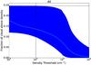 |
Fig. 13 Dense gas mass fraction as a function of volume density threshold n(H2)cm-3. The y-axis shows the sum of 13CO pixels from the GRS cube with H2CO-derived density above the value shown on the x-axis divided by the total. Both values are computed over the velocity range 40 km s-1<vLSR< 75 km s-1. The solid line represents the fraction of 13CO emitting voxels above the mean measured H2CO density as described in Sect. 3.3. The blue shaded region shows the extent of plausible model fits at each density: effectively, this is the ~ 1σ error region. The vertical line at n = 104cm-3 indicates the approximate completeness limit. The horizontal line shows the fraction of 13CO flux in pixels that had corresponding detections at > 2σ in both the H2CO110 − 111 and 211 − 212 lines: it represents the upper limit of what could have been detected if, e.g., all H2CO detections were toward regions with n> 104cm-3. The failure to converge to a fraction f → fmax indicates that there are some real detections of low-density gas. |
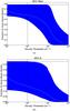 |
Fig. 14 Same as Fig. 13, but for two individual regions: W51 Main a), the region 49.4°<ℓ< 49.6°, − 0.5°<b< − 0.3°, and W51 B b) with 48.8°ℓ< 49.4° and − 0.5°<b< − 0.1°. Note that the y axes have different ranges. The area covered by the W51 B cutout is 6 × larger than the W51 A cutout, so its effect on Fig. 13 is greater. The total area covered in Fig. 13 includes some regions with no detected H2CO, which is why the peak fraction in that figure is lower. |
We also compare the star-forming gas surface density to a 21+24 μm-derived star formation rate surface density in Fig. 16 using standard extragalactic SFR calibrations (Price et al. 2001; Carey et al. 2009; Rieke et al. 2009; Kennicutt & Evans 2012)11. The map was created by filling the saturated regions of the 24 μm MIPS map with empirically scaled 21 μm values. The star formation rate density is only well-correlated with the dense gas surface density in the central portion of W51 A. At lower gas surface densities, the SFR and gas are nearly anticorrelated. This offset is due to an age difference: the gas is tracing star formation yet to begin up to ~ 1 Myr, while the infrared emission traces older (0−100 Myr, with a peak at 5 Myr; Kennicutt & Evans 2012) star formation. The small-scale anticorrelation is consistent with the 5−20′ scales required to recover a star formation law from Galactic plane survey observations (Vutisalchavakul et al. 2014) because of the Kruijssen & Longmore (2014) uncertainty principle for star formation. The improved correlation at the highest densities also implies that the massive star formation threshold is closer to 105cm-3 than the 104cm-3 often measured for nearby, low-mass star-forming regions.
In order to evaluate star formation efficiency as a function of dense gas fraction, a more complete assessment of the present-day or very recent, t< 5 Myr, star formation in the W51 clouds is needed.
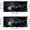 |
Fig. 15 Contours of the dense gas mass fraction using two different thresholds overlaid on the integrated 13CO map. The regions with fraction f> 0.5 should be rapidly forming stars. The background image in both frames is the GRS 13CO image integrated over the range 40 km s-1<vlsr< 75 km s-1, masked to include only pixels with TB> 0.5 K. |
4.2. The future evolution of W51
The low DGMF associated with the W51 B cloud indicates that it has a low star formation potential despite containing significant mass (M ≳ 1 × 10⁵M⊙). The presence of a supernova remnant and old, diffuse H ii regions indicates that the cloud did previously (and recently) form stars, but is now being destroyed. The fact that this cloud contains 10−30% of the total mass of W51, but has only a tiny fraction of its total mass above the purported star forming thresholds supports this story.
This cloud is therefore a good region to examine the effects of different feedback mechanisms (radiation, ionization, and supernovae) in parallel. It may also be a good location to examine how star formation comes to an end in the presence of massive star feedback.
By contrast, the W51 Main region has a dense gas fraction ~ 1 in its center, or at least ~ 50% out to nearly 5 pc. It has presumably only formed a small fraction of its total potential. It exceeds all of the various star formation and massive star formation thresholds (e.g. Lada et al. 2010; Krumholz & McKee 2008; Kauffmann & Pillai 2010), and therefore is expected to form additional stars efficiently, up to ~ 104 − 106M⊙.
4.3. Implications for extragalactic observations of H2CO
Although W51 is one of the most massive and active GMCs in the galaxy, containing 7% of the present-day massive star formation galaxy-wide (Urquhart et al. 2014), its star-forming gas mass is predominantly at a moderate density, n ~ 5 × 104cm-3; there is very little gas above 106cm-3 even in W51 Main. There were no detections of H2CO emission on the ~ 1.25 pc (50′′) scales observed.
The nondetection is not just a geometric effect, as the only gas within W51 that is capable of emitting is tightly associated with the deeply embedded UCH ii regions within W51 Main. The dense gas is spatially compact and very likely to reside along the line of sight toward the continuum sources independent of viewing angle. This geometry is confirmed by existing interferometric observations that also show only absorption (Martin-Pintado et al. 1985a; Arnal & Goss 1985) and observations in other tracers showing that the dense gas is associated on ~ 0.1 pc scales with the UCH ii regions (Zhang & Ho 1997; Zhang et al. 1998).
By contrast, in extragalactic observations of starburst galaxies, there have been detections of H2CO emission on ~ 100 pc scales. Mangum et al. (2013) report detections of H2CO110−111 emission in NGC 3079, IC 860, IR 15107+0724, and Arp 220 on ~ 10 kpc scales. The implied local column densities from their analysis are modest, but the densities are extreme: their observations imply that the local-scale chemical conditions are comparable to W51, but the densities are different.
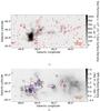 |
Fig. 16 Top: a star-forming gas mass map, created by multiplying the dense gas fraction by the integrated 13CO mass surface density. The red symbols are Class I and flat-spectrum YSOs from Kang et al. (2009) with M< 10 M⊙ (×’s) and M> 10 M⊙ (circles). They are absent from the highest density regions. Bottom: a star formation rate surface density map computed from the MSX 21 cm and MIPS 24 μm (Price et al. 2001; Carey et al. 2009) data with a star formation rate computed using the Rieke et al. (2009) calibration (Kennicutt & Evans 2012). The contours show the star-forming gas surface density above a threshold n> 104cm-3 (red) and n> 105cm-3 (blue) at levels of [100,1000] M⊙ kpc-2. At low star-forming gas surface density, the star formation surface density is essentially anticorrelated with the gas surface density. The two converge at the highest surface densities and at the highest volume densities. |
The only location in which densities n ≳ 5 × 105cm-3 (comparable to n(Arp220), etc.) are observed in W51 are in the central W51 Main region. We do not observe emission because of the bright continuum background source. It is therefore not possible to explain a H2CO-emission galaxy by constructing it from collections of UCH ii regions; such a galaxy would be continuum-bright and show only H2CO absorption. Instead, they must be assembled from huge quantities of high-density, non-star-forming gas. The presence of this gas in turn implies that the density threshold for star formation must be higher in starburst galaxies. This result is in contradiction to the idea that Giant H ii Regions are the building blocks of starburst galaxies (e.g. Miura et al. 2014).
One interpretation of the difference between the Galactic and extragalactic H2CO is that the H ii regions that form in starburst galaxies have their radio luminosity significantly suppressed. The most straightforward explanation for a lower luminosity is that they are smaller and optically thick, compressed by a much more massive and overpressured ISM. Tightly squeezed H ii regions such as these are locations where radiation pressure is likely the dominant form of feedback, with multiple photon scatterings transferring additional momentum to the surrounding medium as described in Murray et al. (2010); this scenario does not occur in the optically thin H ii regions in the Galaxy where ionized gas pressure dominates.
5. Conclusion
We have presented maps of the H2CO110 − 111 and 211 − 212 and H77α and H110α lines covering the W51 star forming complex and used these maps to examine the geometry and density structure of the complex. For the recombination lines, see Appendix A.
The H2CO110 − 111/211 − 212 line ratio was used to measure gas volume densities and dense gas mass fractions. The W51 protoclusters have the majority (> 70%) of their mass in gas with density n(H2) > 5 × 104cm-3. The rest of the cloud has a small dense gas fraction, with f(n> 1 × 104 cm-3) ~ 10%. The W51 B cloud therefore appears to be at the end of its star-forming lifetime, while W51 A will continue to form stars efficiently in the future. The relative weakness of present and future star formation in the W51 B/C region suggests that the collect-and-collapse mechanism is operating inefficiently or not at all.
Present-day high-mass star formation is associated only with W51 A, in which most of the molecular gas has density n ≳ 1 × 105cm-3. The highest gas density is closely associated with bright mid-infrared emission. W51 B and the outskirts of the W51 cloud have some gas with n> 104cm-3, but these regions exhibit limited star formation and show infrared emission anticorrelated with the dense gas. The tighter correlation with massive-star driven star formation indicators at high densities suggests that the density threshold for high-mass star formation is higher than that for low-mass star formation.
The H2CO lines and their ratios have also been used to constrain the geometry of the W51 GMC and the associated H ii regions. The Galactic-face-on view of W51 is presented in more detail than has previously been possible. Analysis of our H2CO data lead to the following conclusions about the structure of the GMC:
-
The high velocity68 km s-1 cloud is infront of the51 km s-1 cloud andthe rest of the W51 GMC complex.
-
The most luminous clusters and associated HII regions are in between the 51 km s-1 and 68 km s-1 clouds.
-
There is molecular absorption associated with W51 B both in front of and behind the W51 C supernova remnant; W51 C is therefore within the W51 B cloud.
It is possible that the foreground 68 km s-1 cloud is falling into the spiral potential from the near side, interacting with the 51 km s-1 cloud exiting the potential on the far side to produce the W51 protoclusters.
Finally, we did not detect any H2CO emission throughout the entire W51 GMC. The nondetection on scales from ~ 1 − 100 pc implies that detections of H2CO110 − 111 emission in other galaxies comes from gas that does not surround bright H ii regions. These galaxies may therefore have interstellar media dominated by very high-density gas (n(H2) > 105.5cm-3) that is not presently forming stars. The density threshold for star formation in these galaxies must therefore be larger than in the Galactic disk, confirming earlier empirical (Longmore et al. 2013) and theoretical (Krumholz et al. 2005; Hennebelle & Chabrier 2013; Padoan & Nordlund 2011) results that such a threshold cannot be universal. These results are inconsistent with a universal density threshold for star formation observed in studies of nearby clouds (Lada et al. 2010, 2012; André et al. 2013).
The data are made available in FITS cubes and images hosted at the CfA dataverse12. The entire reduction and analysis process and all associated code and scripts are made available via a git repository hosted on github13, with a snapshot of the publication version available from zenodo14.
Code Bibliography:
-
The GBT KFPA Pipeline https://safe.nrao.edu/wiki/bin/view/Kbandfpa/ObserverGuide
-
gbtidl http://gbtidl.nrao.edu/
-
astroquery astroquery.readthedocs.org (http://dx.doi.org/10.5281/zenodo.11656)
-
FITS_tools https://github.com/keflavich/FITS_tools
-
aplpy http://aplpy.github.io
-
image-registration http://image-registration.rtfd.org
-
wcsaxes wcsaxes.rtfd.org (>=0.3.dev409)
-
pvextractor pvextractor.rtfd.org
-
pyspeckit pyspeckit.bitbucket.org (Ginsburg & Mirocha 2011)
-
ipython http://ipython.org/ (Pérez & Granger 2007).
Online material
Appendix A: Continuum and RRL data
We compare various data sets to assess calibration uncertainties and provide details of reduction for archival purposes. The data presented in this section are suitable for comparisons of Galactic to extragalactic star formation rate measurements, for example, since they are among the largest angular scale maps of radio recombination lines available with sub-parsec resolution.
Appendix A.1: Comparison between GBT and GPA data
The Galactic Plane A survey (Langston et al. 2000) covered the Galactic plane at 14.35 GHz using the Green Bank Earth Station (GBES) 13.7 m telescope, with a reported FWHM beam size of 6.6′. The published images were released with a FWHM resolution of 8′. We compared our GBT continuum observations to theirs in order to determine whether a significant DC component is missing from our data. Because the GPA used 10deg long scans in Galactic latitude, it should fully recover all diffuse Galactic Plane emission. In the released brightness temperature maps, brightness down to a scale of 1.5deg is recovered. However, because the GPA data undersampled the sky (its 5′ steps between scans were larger than the Nyquist sampling scale of the 14.35 GHz beam), point source fluxes in the GPA are underestimated by 19% and flux on small angular scales may be unreliable.
We resampled the GPA image onto the GBT grid using cubic spline interpolation, then smoothed both data sets to 9.5′. There are image artifacts (particularly vertical streaking) in the GPA data that are diminished by this large smoothing kernel.
We compared the surface brightness in the GPA and GBT data, and found that the GPA data was ~ 0.2 K brighter than the GBT in the diffuse portion of the W51 Main region; the offset
is not consistent with a purely multiplicative offset (Fig. A.1). The GBT observed the W51 Main peak to be moderately brighter, which is likely a result of the sparse sampling in the GPA. The morphological agreement between the maps is imperfect, perhaps in part because of the small area mapped in our GBT data, though there also appears to be vertical (along a line of constant longitude) stretching of the W51 Main source in the unsmoothed GPA data that is not consistent with the GBT observations.
Appendix A.1.1: Comparison between Arecibo and Urumqi data
We compare the 6 cm continuum to the Urumqi 25 m data from Sun et al. (2007) and Sun et al. (2011a). Figure A.2 shows the comparison of the Urumqi data and the Arecibo continuum data smoothed to 9.5′ resolution. The Arecibo and Urumqi data agree well as long as the main beam efficiencies of the respective telescopes (0.5 and 0.67) are accounted for.
Appendix A.1.2: Comparison of GBT and Arecibo data
In order to compare the Green Bank and Arecibo continuum data, we converted the brightness temperature maps to Janskys assuming a beam FWHM of 50′′ for both surveys and central frequencies of 4.8 and 14.5 GHz for Arecibo and Green Bank respectively. Measured beam widths for both telescopes were ~ 49 − 54″, so the relative error from assuming the same beam size should be ≲10%. In this section, the target frequencies are referred to as S5 GHz and S15 GHz for brevity.
The data are well-correlated, with S5 GHz ~ 1.4S15 GHz (S15 GHz ~ 0.7S5 GHz; Fig. A.3), consistent with a spectral index αν = −0.3 slightly steeper than usually observed for optically
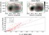 |
Fig. A.1 Comparison between the GBT and NRAO GBES (Langston et al. 2000) data. Top left: NRAO GBES 2 cm map (top right) GBT 2 cm map of the same region smoothed to about 8.9′. The colorbar applies to both figures, showing brightness temperature units in K. The red contours in both figures show the region observed by Green Bank; flux outside of those boundaries is extrapolated with the smoothing kernel. The green contours show the region where TB(GBT) >TB(GBES). Bottom: plot of the GBT vs. the GBES surface brightness measurements. The large red dots show the region within the red contours. |
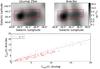 |
Fig. A.2 Comparison between the Arecibo and Urumqi 25 m (Sun et al. 2011b) data. Top left: Urumqi 6 cm map of the W51 region. Top right: Arecibo 6 cm map of the same region smoothed to the 9.5′ resolution of the Urumqi data set. The colorbar applies to both figures, showing brightness temperature units in K. The red contours in both figures show the region observed by Arecibo; flux outside of those boundaries is extrapolated with the smoothing kernel. Bottom: plot of the Arecibo vs. the Urumqi surface brightness measurements. The red dots show the region within the red contours. |
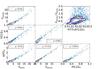 |
Fig. A.3 5 GHz and 15 GHz continuum and RRL flux densities against one another; all units are in Jy. The dashed lines show the total least squares best fit line with the slope shown in the legend. Wherever the density of points is too high to display, the points have been replaced with a contour plot showing the density of data points. The upper-right panel shows a comparison of the continuum ratio to the RRL ratio. The dashed line in the upper-right plot has slope 1, and the dotted line has slope 0.6. |
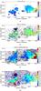 |
Fig. A.4 Ratio maps of the ionized gas in W51. a) Continuum ratio S15 GHz/S5 GHz. For α = −0.1, an optically thin free-free source, the ratio is 0.9, while for α = 2, an optically thick source, the ratio is 9. b) The ratio of the H77α peak to the H112α peak. c) The line-to-continuum ratio H112α/S5 GHz. d) The line-to-continuum ratio H77α/S15 GHz. |
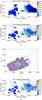 |
Fig. A.5 a) H112α electron temperature map showing |
thin brehmsstrahlung and consistent with there being some contribution from synchrotron emission. The lower-brightness regions have a lower S15 GHz/S5 GHz, indicating that these regions are more affected by synchrotron. In Fig. A.4a, a great deal of structure in the S15 GHz/S5 GHz ratio is evident in the vicinity of W51 Main: the ratio is higher towards the continuum peaks, indicating that the peaks have higher free-free optical depths, or lower relative contributions from synchrotron emission, than their envelopes.
We additionally compare the radio recombination lines observed simultaneously with the continuum and H2CO. Hydrogen RRLs are often extremely well-correlated with the continuum and are therefore good indicators of the calibration quality.
In Fig. A.4, we show the ratios between the two frequencies in RRLs and continuum and the line-to-continuum ratios at both frequencies. The line values are the integrated flux densities over the range 20 to 100 km s-1, which includes all Hα emission but no Heα.
The ratios between the x and y axis in each plot in Fig. A.3 are fitted using a total least squares approach with uniform errors for each data point. The line-to-continuum ratio is L/C(H77α) ~ 0.15 and L/C(H112α) ~ 0.04; in both cases there is little evidence for deviation from a linear relationship.
Appendix A.1.3: Comparison of the RRL and continuum data
Radio recombination lines are generally observed to be well-correlated with the corresponding radio continuum, particularly at low frequencies. At 5 and 15 GHz, the population level departure coefficients are close to 1, bn> 0.95 (Wilson et al. 2009; Walmsley 1990).
While radio recombination lines are purely thermal in nature, the large-scale continuum may include a contribution from synchrotron emission. The morphological similarity between the 90 cm and 4 m (meter – i.e., 74 MHz) images presented by Brogan et al. (2013) and our 6 and 2 cm data hint that synchrotron emission could be significant. However, the high degree of correlation between the 2 and 6 cm described below suggest that synchrotron contamination is minor at both wavelengths.
Figure A.3 shows a comparison between the integrated RRL surface brightness and radio continuum at both 2 and 6 cm15. The figure shows the total least squares best-fit slopes to the data assuming uniform error, which yield a measurement of the line-to-continuum ratio.
We use the line-to-continuum ratio in both bands to measure the electron temperature using Eq. (14.58) of Wilson et al. (2009), which assumes a plane-parallel, optically-thin emission region with lines formed in local thermodynamic equilibrium (the ∗ in  is meant to indicate these three assumptions are made). The two lines yield consistent measurements, with mean
  K; these measurements are consistent with smaller-scale measurements using the VLA with H92α (Mehringer 1994). There is little structure in the maps, with a hint of higher temperatures around G49.1-0.4, coincident with the W51C supernova remnant. Other structures are most likely due to the limited S/N.
Finally, we fit a single-component Gaussian to each pixel to produce velocity maps. These are discussed in Sect. B.11.
Appendix A.2: Carbon and helium RRLs
Helium RRLs were prevalent and reasonably well-correlated with the hydrogen RRLs, but we did not examine them in detail. He77α is detected at much higher S/N than than He107-112α. There were no clear detections of C77α or C107-112α, though there is a possible C77α signal at G49.366-0.304 with vlsr ≈ 55 km s-1 and a possible detection toward W51 Main along the wing of the He77α line. The He77α line detections are associated with regions of high Hnα but not regions of different .
Appendix B: Geometry of individual regions
Appendix B.1: W51 main and W51 IRS 2
The W51 main and IRS 2 spectra show that both have ionized gas components at vLSR ~ 55 km s-1. This velocity approximately coincides with the peak of the 13CO emission.
The H2CO110 − 111 spectra are deepest at ~ 68 km s-1, while the 211 − 212 have depths approximately equal between the ~ 58 km s-1 and ~ 68 km s-1 components. The 55−60 km s-1 components are too deep to be entirely behind the H ii regions. This indicates that the 55 km s-1 ionized gas must be embedded within the molecular cloud, with molecular gas on both sides of the ionized gas along the line of sight.
Because these are well-studied regions, the low spatial resolution H2CO spectra we present here add little new information about the gas kinematics. However, all of the velocity components observed in the W51 region are apparently kinematically connected to the W51 clusters.
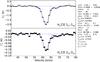 |
Fig. B.1 Spectrum extracted from G49.119-0.277 in a 55′′ radius aperture, showing a model in which the continuum is behind the 63 km s-1 component but in front of the 68 km s-1 component. The legend gives the fit parameters along with 1σ error bars. The parameters with no errors indicated (OPR, T, TBG) are assumed or independently measured values. |
Appendix B.2: The W51 B filament
The W51 B filament (right side of Fig. 11 at ~ 68 km s-1), exhibits bright CO emission ( K in the Parsons et al. 2012 CO 3−2 data) but has relatively weak H2CO absorption. The absorption models are inconsistent with the molecular gas being in front of the continuum emission, so Fig. 11 shows the continuum sources in front of the cloud at lower ℓ. Figure 8 shows an example model fit with the continuum assumed to be in front and in back, illustrating that the best-fit model parameters with continuum in the back do not reproduce the data. The relative positioning of the molecular gas behind the H ii regions suggests that the molecular gas is also behind the W51 C supernova remnant.
Appendix B.3: The edge of W51 C
W51 C is a supernova remnant that spatially overlaps with the W51 B star forming region. Brogan et al. (2013) argue that the supernova remnant must be in front of the H ii region G49.20-0.35 because the H ii-region has not absorbed all of the 4 m (74 MHz) nonthermal emission. The G49.1-0.4, G49.0-0.3, and G48.9-0.3 regions, however, show 4 m absorption signatures and may be in the foreground. There are clumps aligned along the 68 km s-1 filamentary cloud with very high CO and H i velocities (Koo & Moon 1997b,a; Brogan et al. 2013), indicating that the SNR is interacting with the molecular gas.
The clumps at G49.1-0.3, ~ 68 km s-1 are either lower density (n< 1.5 × 104cm-3) and in the background of the H ii region or high density (n> 1.5 × 105cm-3), low-column density and in the foreground. The 62 km s-1 clumps have densities a few times higher, n ~ 4 × 104cm-3, and are clearly in the foreground of the continuum emission because their absorption depths are ~ 2.5 K, which cannot occur for absorption against the CMB. Figure B.1 shows a model spectrum fitted assuming the continuum lies between the two molecular velocity components. The relative strength of the 13CO and the H2CO also suggests that the 68 km s-1 component is behind the continuum.
We are seeing molecular gas both in front of and behind the supernova. This geometry can be readily confirmed by looking for molecular absorption at much lower frequencies where the SN synchrotron emission dominates over the H ii region free-free emission, i.e. the 335 and 71 MHz p - H2CO lines.
Appendix B.4: G49.20-0.35 and G49.1-0.4
Tian & Leahy (2013) focus on the H ii regions G49.20-0.35 and G49.10-0.40 (called G49.10-0.38 in their work) to determine the relative geometry of the W51 C SNR and the W51 B H ii/star-forming region. They observe that the high-velocity H iis not detected toward either of these sources, indicating that the H ii regions must be behind the high-velocity H i features.
We detect H2CO110 − 111 at ~ 58 and ~ 63 km s-1 toward G49.10-0.40, with line ratios that are consistent with the H ii region being behind the molecular cloud complex. It also has an extreme RRL velocity, v110α ≈ 72 km s-1, the most redshifted seen in the entire W51 region (see Figs. B.3 and B.2).
G49.20-0.35 is also clearly behind the molecular cloud, as evidenced both by H2CO absorption depth and the IRDC absorption in the foreground. It has an RRL velocity v110α ≈ 70 km s-1.
Because both H ii regions are extremely redshifted, they are most likely associated with the W51 B cloud complex, contrary to the interpretation by Tian & Leahy (2013) in which they are unrelated background clouds. The Galactic rotation curve doesn’t allow for velocities red of ~ 60 km s-1, and almost none of the molecular gas exceeds ~ 70 km s-1 even on the wings. The H ii regions are therefore probably shooting out the back side of the molecular cloud in a champagne flow, perhaps accelerating ionized gas from the ~ 68 km s-1 component further to the red.
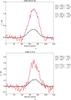 |
Fig. B.2 Fitted H110α (red) and H77α (black) spectra extracted from 55′′ apertures centered on G49.20-0.35 (top) and G49.1-0.4 (bottom). The best-fit Gaussian parameters are shown in the legends, with the lower legend corresponding to H77α. |
Appendix B.5: The 66 km s-1 8 μm dark cloud
Between W51 A and W51 B, there is a component of the 68 km s-1 cloud that is filamentary and in the foreground of all of the free-free emission. This cloud component is evident as an IRDC in the Spitzer GLIMPSE images from ℓ = 49.393, b = −0.357 to ℓ = 49.207, b = −0.338; it is labeled as IRDC G49.37-0.35 in Figs. 11 and 12.
The H ii region G49.20-0.35 is clearly behind the IRDC, though there are strong morphological hints that it is interacting with and truncated by the cloud.
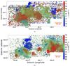 |
Fig. B.3 a) Velocity of the peak H2CO110 − 111 signal (deepest absorption) at 1 km s-1 resolution. b) Velocity of the peak H110α emission as derived from Gaussian fits to each spectrum. |
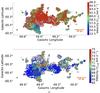 |
Fig. B.4 Maps of the fitted H2CO velocity components over the range 40 <vLSR< 66 km s-1 (left) and 66 <vLSR< 75 km s-1 (right). The regions that appear noisy have ambiguous multi-component decompositions. |
Appendix B.6: G49.27-0.34
The UCH ii region G49.27-0.34, which was considered a candidate extended green object (EGO) and subsequently rejected for lack of H2 emission (De Buizer & Vacca 2010; Lee et al. 2013), exhibits a second velocity component at ~ 68 km s-1, slightly but clearly redshifted of the rest of the IRDC. The dust component contains a gas mass ~ 2 × 10³M⊙ based on the BGPS flux and using the assumptions outlined in Aguirre et al. (2011), suggesting that the high velocity could be due to infall or virialized gas within a deep potential. The virialized velocity width, given the radius and mass from the BGPS data, is σvir = 8.8 km s-1, while the measured H2CO linewidth is FWHM(H2CO) = 7.2 km s-1, wider than in any other part of the cloud except W51 Main.
Both radio continuum and RRLs are detected toward this source. The H77α RRL velocity is ~ 58 km s-1, significantly blueshifted from the molecular gas. The H2CO lines do not independently distinguish between the continuum source being in the front or back of the cloud, but the mean density from the BGPS mass and radius n ~ 2.5 × 104cm-3 is within a factor of 2 of the H2CO-derived density, n ~ 1.4 × 104cm-3, if the continuum source is behind the gas, while the H2CO-derived density is too low, n ~ 2 × 103cm-3 if the continuum source is in front.
The implied geometry therefore has the H ii region behind the molecular gas, plowing toward it at a velocity difference Δv ~ 10 km s-1. Such a high velocity difference may indicate that the H ii region is confined by the molecular gas and on a plunging orbit into the cloud.
Appendix B.7: G49.4-0.3f, aka G49.34-0.34, aka IRAS 19209+1418
The H ii region centered at 49.34-0.34 was identified by Mehringer (1994) as part of the G49.4-0.3 complex. There are 3 distinct H2CO line components at 51, 63.70, and 68.47 km s-1. The 51 km s-1 component is behind the H ii region; the 13CO line is detected at comparable brightness at 51 km s-1 and 63 km s-1, while the H2CO110 − 111 line is ~ 10 × deeper at 63 km s-1. The RRLs associated with this source are at vLSR = 58 ± 1 km s-1.
The H2CO lines are moderately well-fit by the two-velocity-component model, but there is a relative excess of 211 − 212 absorption at 66 km s-1 (associated with the 68 km s-1 component). The extra absorption may indicate that there is a high-density, low-column component at this velocity.
The 8 μm GLIMPSE image shows that the 68 km s-1 IRDC crosses in front of this source. Herschel Hi-Gal 70 μm images reveal a ring structure that is hinted at in the 8 μm image. There is no evidence for interaction between the ring feature and the IRDC. This intriguing feature will likely be difficult to study in detail because the dusty, molecular gas feature lies in front of it.
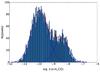 |
Fig. B.5 A histogram of the abundances derived for each spatial pixel using the LVG grid fit. The abundance shown assumes a velocity gradient 1 km s-1pc-1. The overlaid fits show that 30% of the area of W51 is consistent with an abundance X(o - H2CO) = 10− 8.4 ± 0.5 and 70% with X(o - H2CO) = 10− 9.9 ± 0.6. |
Appendix B.8: G49.4-0.3
The collection of H ii regions around G49.4-0.3 vaguely resembles a cartoon mouse. As noted in Carpenter & Sanders (1998), the molecular gas in this region is separated into two distinct components, one at 51 km s-1 and the other at 64 km s-1. The 64 km s-1 component is in the foreground, while the 51 km s-1 is in the background of most of the H ii regions.
Both cloud components are in the foreground of the central H ii regions at G49.36-0.31, the eyes of the mouse. The density of the 51 km s-1 component is an order of magnitude higher than that in the 64 km s-1 component in this region, suggesting that the gas is being compressed by the H ii region. The clean separation between the 64 and 51 km s-1 cloud components suggests that they are not interacting at this location.
Based on the absorption line depths, the G49.38-0.30, IRAS 19207+1422, and G49.37-0.30 H ii regions are behind the 51 km s-1 cloud. The 8 μm absorption features are associated with the 64 km s-1 cloud and are in front of all of the H ii regions.
The 8 μm morphology of G49.42-0.31 is bubble-like, so it is plausible that the H ii region is neither in front nor behind the 51 km s-1 cloud but embedded within it, blowing a hole in the cloud.
Appendix B.9: 8 μm dark cloud G49.47-0.27
The cloud to the north of W51 Main/IRS2 appears as a dark feature in Spitzer GLIMPSE 8 μm maps. It is detected in H2CO from 54 to 64 km s-1. Throughout, it has a high 110 − 111/211 − 212 ratio, ≳7 in most voxels, indicating a low density n ≲ 103cm-3.
Centered at 60.6 km s-1, the region has a line FWHM 5−7 km s-1, indicating that it is quite turbulent, with 3D Mach number in the range 10 < ℳ < 20 for an assumed 10 <T< 20 K. At its centroid velocity, it is connected to the W51 main cloud.
There is a previously unreported bubble HII region in the north part of this cloud, which we designate G49.47-0.26, with radius ~ 70″ (1.7 pc). The H ii has RRL velocities vlsr ≈ 50 km s-1. Because it is not detected in Brackett γ emission (from the UWISH2 survey: Froebrich et al. 2011), it is most likely behind the cloud.
The Kang et al. (2009)Spitzer survey of YSOs in the region indicates that there are no YSOs within the boundaries of this cloud; it is very likely non-star-forming at present (see also Fig. 16).
Because the cloud is continuous with the W51 Main region in velocity and is 8 μm-dark, it is most likely at the same distance as W51 Main and associated indirectly with the massive cluster forming region.
Appendix B.10: The 40 km s-1 clouds
There are clouds observed at 40 km s-1 that show only weak H2CO absorption spread across nearly the entire region. These molecular clouds are behind nearly all of the H ii regions in the W51 complex. There are additional 40 km s-1 clouds clearly seen in H i absorption (Stil et al. 2006) that are not associated with these molecular clouds, but instead represent a foreground population of neutral atomic medium clouds.
Appendix B.11: Kinematic maps
Maps showing the overall kinematics of the region are shown in Figs. B.3 and B.4. Figure B.3 shows the velocity at peak absorption of the H2CO110 − 111 line and the fitted radio recombination line centroid velocity. Figure B.4 shows the best simultaneous fit to the H2CO110 − 111 and 211 − 212 absorption features over two different velocity ranges. The 110 − 111 absorption velocity in Fig. B.3a approximately shows the velocity of the front-most molecular clouds along the line of sight at each position.
Appendix B.12: Abundances
The LVG modeling also yields measurements of abundance that are degenerate with the assumed velocity gradient. The abundance within the LVG model is defined as ![\appendix \setcounter{section}{2} \begin{equation} X = \frac{N(\ortho) \left[\persc \left/ \left(\kms\,\perpc\right)\right]\right.}{n(\hh) \left[\percc\right]} \left(\frac{1~\kms\,\perpc}{\mathrm{pc}}\right)\cdot \end{equation}](/articles/aa/full_html/2015/01/aa24979-14/aa24979-14-eq213.png) (B.1)\newpage\noindentWe show the distribution of fitted abundances under this definition in Fig. B.5. The histogram shows the average abundance along each line of sight derived from the likelihood-weighted density divided by the likelihood-weighted column. We also show a two-gaussian fit to the abundance distribution: 30% of the area is consistent with an abundance X(o - H2CO) = 10− 8.4 ± 0.5 and 70% with X(o - H2CO) = 10− 9.9 ± 0.6. We caution that these abundance measurements are highly uncertain and are contingent on both the backlighting source brightness and the assumed velocity gradient. The individual abundances going in to the histogram are generally not well-constrained. A more accurate abundance measurement could be obtained by measuring the millimeter lines of o - H2CO at 140 and 150 GHz.
(B.1)\newpage\noindentWe show the distribution of fitted abundances under this definition in Fig. B.5. The histogram shows the average abundance along each line of sight derived from the likelihood-weighted density divided by the likelihood-weighted column. We also show a two-gaussian fit to the abundance distribution: 30% of the area is consistent with an abundance X(o - H2CO) = 10− 8.4 ± 0.5 and 70% with X(o - H2CO) = 10− 9.9 ± 0.6. We caution that these abundance measurements are highly uncertain and are contingent on both the backlighting source brightness and the assumed velocity gradient. The individual abundances going in to the histogram are generally not well-constrained. A more accurate abundance measurement could be obtained by measuring the millimeter lines of o - H2CO at 140 and 150 GHz.
Appendix B.13: Supplementary picture
We include a large-scale WISE + BGPS composite image of the entire W51 cloud and its surroundings. The figure highlights the W51 C supernova remnant.
 |
Fig. B.6 A large-scale color composite that highlights the W51 C supernova remnant as a white haze using 90 cm data from Brogan et al. (2013). The colors are the same as in Fig. 1: the blue, green, and red colors are WISE bands 1, 3, and 4 (3.4, 12, and 22 μm) respectively. The yellow-orange semitransparent layer is from the Bolocam 1.1 mm Galactic Plane Survey data (Aguirre et al. 2011; this paper). |
The midplane at d = 5.1 kpc is offset approximately − 0.22 to − 0.33 degrees from b = 0 depending on our solar system’s height above the midplane, Z⊙ = 20 pc or 30 pc, respectively (Reed 2006; Joshi 2007).
Higher frequency H2CO lines show the same behavior, though the effect is progressively weaker; see Darling & Zeiger (2012) Fig. 2.
The data can be retrieved from within aoIDL with the command n=mmgetarchive(yymmdd1,yymmdd2,mm,rcvnum=9), then the ηMB data are in mm.fit.etamb. The calibration process is recorded in detail in Heiles et al. (2001).
This is a simplification; other factors in the weight include the optical depth for an optically thick line, the abundance of H2CO, and the geometry if there is a background source. For most of the W51 cloud, a fixed abundance and optically thin lines are not a bad assumption, and we account for the geometry in the discussion.
Acknowledgments
We thank Xiaohui Sun for providing the Urumqi 6 cm Stokes I image prior to its availability on the survey website. The paper benefitted from discussions with Jonathan Tan, Neal Evans, and Diederik Kruijssen. We thank our referee Jeff Mangum for a helpful and rapid referee report. We are grateful to the editor, Malcolm Walmsley, for additional comments and for catching many small but significant errors. E.R. is supported by a Discovery Grant from NSERC of Canada. This research has made use of the VizieR catalogue access tool, CDS, Strasbourg, France. The original description of the VizieR service was published in (Ochsenbein et al. 2000). This publication makes use of molecular line data from the Boston University-FCRAO Galactic Ring Survey (GRS). The GRS is a joint project of Boston University and Five College Radio Astronomy Observatory, funded by the National Science Foundation under grants AST-9800334, AST-0098562, AST-0100793, AST-0228993, & AST-0507657. This research has made use of the NASA/ IPAC Infrared Science Archive, which is operated by the Jet Propulsion Laboratory, California Institute of Technology, under contract with the National Aeronautics and Space Administration.
References
- Aguirre, J. E., Ginsburg, A. G., Dunham, M. K., et al. 2011, ApJS, 192, 4 [NASA ADS] [CrossRef] [MathSciNet] [Google Scholar]
- André, P., Francesco, J. D., Ward-Thompson, D., et al. 2013, Protostars and Planet VI (University of Arizona Press), accepted [arXiv:1312.6232] [Google Scholar]
- Ao, Y., Henkel, C., Menten, K. M., et al. 2013, A&A, 550, A135 [NASA ADS] [CrossRef] [EDP Sciences] [Google Scholar]
- Arnal, E. M., & Goss, W. M. 1985, A&A, 145, 369 [NASA ADS] [Google Scholar]
- Astropy Collaboration, Robitaille, T. P., Tollerud, E. J., et al. 2013, A&A, 558, A33 [NASA ADS] [CrossRef] [EDP Sciences] [Google Scholar]
- Bastian, N. 2008, MNRAS, 390, 759 [NASA ADS] [CrossRef] [Google Scholar]
- Battersby, C., Bally, J., Dunham, M., et al. 2014, ApJ, 786, 116 [NASA ADS] [CrossRef] [Google Scholar]
- Battisti, A. J., & Heyer, M. H. 2014, ApJ, 780, 173 [NASA ADS] [CrossRef] [EDP Sciences] [Google Scholar]
- Beaumont, C. N., Offner, S. S. R., Shetty, R., Glover, S. C. O., & Goodman, A. A. 2013, ApJ, 777, 20 [Google Scholar]
- Beccari, G., Spezzi, L., De Marchi, G., et al. 2010, ApJ, 720, 1108 [NASA ADS] [CrossRef] [Google Scholar]
- Bieging, J. H., Peters, W. L., & Kang, M. 2010, ApJS, 191, 232 [NASA ADS] [CrossRef] [Google Scholar]
- Bressert, E., Ginsburg, A., Bally, J., et al. 2012, ApJ, 758, L28 [NASA ADS] [CrossRef] [Google Scholar]
- Brogan, C. L., Frail, D. A., Goss, W. M., & Troland, T. H. 2000, ApJ, 537, 875 [NASA ADS] [CrossRef] [Google Scholar]
- Brogan, C. L., Goss, W. M., Hunter, T. R., et al. 2013, ApJ, 771, 91 [Google Scholar]
- Burkert, A., & Hartmann, L. 2013, ApJ, 773, 48 [NASA ADS] [CrossRef] [Google Scholar]
- Carey, S. J., Noriega-Crespo, A., Mizuno, D. R., et al. 2009, PASP, 121, 76 [NASA ADS] [CrossRef] [Google Scholar]
- Carpenter, J. M., & Sanders, D. B. 1998, AJ, 116, 1856 [NASA ADS] [CrossRef] [Google Scholar]
- Clark, P. C., & Glover, S. C. O. 2013 [Google Scholar]
- Dale, J. E., & Bonnell, I. A. 2008, MNRAS, 391, 2 [NASA ADS] [CrossRef] [Google Scholar]
- Dale, J. E., Bonnell, I. A., Clarke, C. J., & Bate, M. R. 2005, MNRAS, 358, 291 [NASA ADS] [CrossRef] [MathSciNet] [Google Scholar]
- Dale, J. E., Ercolano, B., & Bonnell, I. A. 2012, MNRAS, 427, 2852 [NASA ADS] [CrossRef] [Google Scholar]
- Dale, J. E., Ngoumou, J., Ercolano, B., & Bonnell, I. A. 2013, MNRAS, 436, 3430 [NASA ADS] [CrossRef] [Google Scholar]
- Darling, J., & Zeiger, B. 2012, ApJ, 749, L33 [NASA ADS] [CrossRef] [Google Scholar]
- Davies, B. 2012, in Proc. of a Scientific Meeting in Honor of Anthony F. J. Moffat, eds. L. Drissen, C. Rubert, N. St.-Louis, & A. F. J. Moffat, ASP Conf. Ser., 465, 383 [Google Scholar]
- De Buizer, J. M., & Vacca, W. D. 2010, AJ, 140, 196 [NASA ADS] [CrossRef] [Google Scholar]
- Froebrich, D., Davis, C. J., Ioannidis, G., et al. 2011, MNRAS, 413, 480 [NASA ADS] [CrossRef] [Google Scholar]
- Ginsburg, A., & Mirocha, J. 2011, Astrophysics Source Code Library, 9001 [Google Scholar]
- Ginsburg, A., Darling, J., Battersby, C., Zeiger, B., & Bally, J. 2011, ApJ, 736, 149 [NASA ADS] [CrossRef] [Google Scholar]
- Ginsburg, A., Bressert, E., Bally, J., & Battersby, C. 2012, ApJ, 758, L29 [NASA ADS] [CrossRef] [Google Scholar]
- Green, S. 1991, ApJS, 76, 979 [NASA ADS] [CrossRef] [Google Scholar]
- Heiles, C., Perillat, P., Nolan, M., et al. 2001, PASP, 113, 1247 [NASA ADS] [CrossRef] [Google Scholar]
- Henkel, C., Walmsley, C. M., & Wilson, T. L. 1980, A&A, 82, 41 [NASA ADS] [Google Scholar]
- Hennebelle, P., & Chabrier, G. 2011, ApJ, 743, L29 [NASA ADS] [CrossRef] [Google Scholar]
- Hennebelle, P., & Chabrier, G. 2013, ApJ, 770, 150 [NASA ADS] [CrossRef] [Google Scholar]
- Hopkins, P. F., Narayanan, D., Murray, N., & Quataert, E. 2013, MNRAS, 433, 69 [NASA ADS] [CrossRef] [Google Scholar]
- Jackson, J. M., Rathborne, J. M., Shah, R. Y., et al. 2006, ApJS, 163, 145 [NASA ADS] [CrossRef] [Google Scholar]
- Joshi, Y. C. 2007, MNRAS, 378, 768 [NASA ADS] [CrossRef] [Google Scholar]
- Juneau, S., Narayanan, D. T., Moustakas, J., et al. 2009, ApJ, 707, 1217 [NASA ADS] [CrossRef] [Google Scholar]
- Kainulainen, J., Federrath, C., & Henning, T. 2013, A&A, 553, L8 [Google Scholar]
- Kalirai, J. S., & Richer, H. B. 2010, Roy. Soc. London Philos. Trans. Ser. A, 368, 755 [NASA ADS] [CrossRef] [Google Scholar]
- Kang, M., Bieging, J. H., Povich, M. S., & Lee, Y. 2009, ApJ, 706, 83 [NASA ADS] [CrossRef] [Google Scholar]
- Kang, M., Bieging, J. H., Kulesa, C. A., et al. 2010, ApJS, 190, 58 [NASA ADS] [CrossRef] [Google Scholar]
- Kauffmann, J., & Pillai, T. 2010, ApJ, 723, L7 [NASA ADS] [CrossRef] [Google Scholar]
- Kennicutt, R. C., & Evans, N. J. 2012, ARA&A, 50, 531 [NASA ADS] [CrossRef] [Google Scholar]
- Koo, B.-C., Kim, K.-T., & Seward, F. D. 1995, ApJ, 447, 211 [Google Scholar]
- Koo, B.-C., & Moon, D.-S. 1997a, ApJ, 475, 194 [Google Scholar]
- Koo, B.-C., & Moon, D.-S. 1997b, ApJ, 485, 263 [Google Scholar]
- Kruijssen, J. M. D. 2012, MNRAS, 426, 3008 [NASA ADS] [CrossRef] [Google Scholar]
- Kruijssen, J. M. D. 2014, MNRAS, 440, 3370 [NASA ADS] [CrossRef] [Google Scholar]
- Kruijssen, J. M. D., & Longmore, S. N. 2014, MNRAS, 439, 3239 [NASA ADS] [CrossRef] [Google Scholar]
- Krumholz, M. R., & McKee, C. F. 2008, Nature, 451, 1082 [NASA ADS] [CrossRef] [PubMed] [Google Scholar]
- Krumholz, M. R., McKee, C. F., & Klein, R. I. 2005, Nature, 438, 332 [NASA ADS] [CrossRef] [PubMed] [Google Scholar]
- Krumholz, M. R., Klein, R. I., & McKee, C. F. 2007, ApJ, 665, 478 [NASA ADS] [CrossRef] [Google Scholar]
- Krumholz, M. R., Bate, M. R., Arce, H. G., et al. 2014, Protostars and Planet VI (University of Arizona Press), accepted [arXiv:1401.2473] [Google Scholar]
- Kudryavtseva, N., Brandner, W., Gennaro, M., et al. 2012, ApJ, 750, L44 [NASA ADS] [CrossRef] [Google Scholar]
- Lada, C. J., Lombardi, M., & Alves, J. F. 2010, ApJ, 724, 687 [NASA ADS] [CrossRef] [Google Scholar]
- Lada, C. J., Forbrich, J., Lombardi, M., & Alves, J. F. 2012, ApJ, 745, 190 [NASA ADS] [CrossRef] [Google Scholar]
- Langer, W. D., Velusamy, T., Pineda, J. L., Willacy, K., & Goldsmith, P. F. 2014, A&A, 561, A122 [NASA ADS] [CrossRef] [EDP Sciences] [Google Scholar]
- Langston, G., Minter, A., D’Addario, L., et al. 2000, AJ, 119, 2801 [NASA ADS] [CrossRef] [Google Scholar]
- Lee, K. I., Looney, L. W., Schnee, S., & Li, Z.-Y. 2013 [Google Scholar]
- Longmore, S. N., Bally, J., Testi, L., et al. 2012, ApJ, 746, 117 [NASA ADS] [CrossRef] [Google Scholar]
- Longmore, S. N., Bally, J., Testi, L., et al. 2013, MNRAS, 429, 987 [NASA ADS] [CrossRef] [Google Scholar]
- Longmore, S. N., Bally, J., Testi, L., et al. 2014, MNRAS, 433, L15 [Google Scholar]
- Mangum, J. G., & Wootten, A. 1993, ApJS, 89, 123 [NASA ADS] [CrossRef] [Google Scholar]
- Mangum, J. G., Emerson, D. T., & Greisen, E. W. 2007, A&A, 474, 679 [NASA ADS] [CrossRef] [EDP Sciences] [Google Scholar]
- Mangum, J. G., Darling, J., Henkel, C., & Menten, K. M. 2013, ApJ, 766, 108 [NASA ADS] [CrossRef] [Google Scholar]
- Martin-Pintado, J., Wilson, T. L., Henkel, C., & Gardner, F. F. 1985a, A&A, 142, 131 [NASA ADS] [Google Scholar]
- Martin-Pintado, J., Wilson, T. L., Johnston, K. J., & Henkel, C. 1985b, ApJ, 299, 386 [NASA ADS] [CrossRef] [Google Scholar]
- Mehringer, D. M. 1994, ApJS, 91, 713 [NASA ADS] [CrossRef] [Google Scholar]
- Miura, R. E., Kohno, K., Tosaki, T., et al. 2014, ApJ, 788, 167 [NASA ADS] [CrossRef] [Google Scholar]
- Muraoka, K., Kohno, K., Tosaki, T., et al. 2009, PASJ, 61, 163 [NASA ADS] [Google Scholar]
- Murray, N., Quataert, E., & Thompson, T. A. 2010, ApJ, 709, 191 [NASA ADS] [CrossRef] [Google Scholar]
- Myers, A., Klein, R., Krumholz, M., & McKee, C. 2014, MNRAS, 439, 3420 [NASA ADS] [CrossRef] [Google Scholar]
- Ochsenbein, F., Bauer, P., & Marcout, J. 2000, A&AS, 143, 23 [NASA ADS] [CrossRef] [EDP Sciences] [Google Scholar]
- Padoan, P., & Nordlund, Å. 2011, ApJ, 730, 40 [NASA ADS] [CrossRef] [Google Scholar]
- Padoan, P., Federrath, C., Chabrier, G., et al. 2014, in Protostars and Planets VI (University of Arizona Press), eds. H. Beuther, et al. [arXiv:1312.5365] [Google Scholar]
- Parker, R. J., & Dale, J. E. 2013 [Google Scholar]
- Parmentier, G. 2011, MNRAS, 413, 1899 [NASA ADS] [CrossRef] [Google Scholar]
- Parmentier, G., Kauffmann, J., Pillai, T., & Menten, K. M. 2011, MNRAS, 416, 783 [NASA ADS] [Google Scholar]
- Parsons, H., Thompson, M. A., Clark, J. S., & Chrysostomou, A. 2012, MNRAS, 424, 1658 [NASA ADS] [CrossRef] [Google Scholar]
- Pérez, F., & Granger, B. E. 2007, Comput. Sci. Eng., 9, 21 [Google Scholar]
- Pineda, J. E., & Teixeira, P. S. 2013, A&A, 555, A106 [NASA ADS] [CrossRef] [EDP Sciences] [Google Scholar]
- Price, S. D., Egan, M. P., Carey, S. J., Mizuno, D. R., & Kuchar, T. A. 2001, AJ, 121, 2819 [NASA ADS] [CrossRef] [Google Scholar]
- Reed, B. C. 2006, JRASC, 100, 146 [NASA ADS] [Google Scholar]
- Rieke, G. H., Alonso-Herrero, A., Weiner, B. J., et al. 2009, ApJ, 692, 556 [NASA ADS] [CrossRef] [Google Scholar]
- Rogers, H., & Pittard, J. M. 2013, MNRAS, 431, 1337 [NASA ADS] [CrossRef] [Google Scholar]
- Sato, M., Reid, M. J., Brunthaler, A., & Menten, K. M. 2010, ApJ, 720, 1055 [NASA ADS] [CrossRef] [Google Scholar]
- Smith, R. J., Glover, S. C. O., Clark, P. C., Klessen, R. S., & Springel, V. 2014, MNRAS, 441, 1628 [NASA ADS] [CrossRef] [Google Scholar]
- Stil, J. M., Taylor, A. R., Dickey, J. M., et al. 2006, AJ, 132, 1158 [NASA ADS] [CrossRef] [Google Scholar]
- Sun, X. H., Han, J. L., Reich, W., et al. 2007, A&A, 463, 993 [NASA ADS] [CrossRef] [EDP Sciences] [Google Scholar]
- Sun, X. H., Reich, P., Reich, W., et al. 2011a, A&A, 536, A83 [NASA ADS] [CrossRef] [EDP Sciences] [Google Scholar]
- Sun, X. H., Reich, W., Han, J. L., et al. 2011b, A&A, 527, A74 [NASA ADS] [CrossRef] [EDP Sciences] [Google Scholar]
- Tian, W. W., & Leahy, D. A. 2013, ApJ, 769, L17 [Google Scholar]
- Troscompt, N., Faure, A., Wiesenfeld, L., Ceccarelli, C., & Valiron, P. 2009, A&A, 493, 687 [NASA ADS] [CrossRef] [EDP Sciences] [Google Scholar]
- Urquhart, J. S., Figura, C. C., Moore, T. J. T., et al. 2014, MNRAS, 437, 1791 [NASA ADS] [CrossRef] [Google Scholar]
- van der Tak, F. F. S., Black, J. H., Schöier, F. L., Jansen, D. J., & van Dishoeck, E. F. 2007, A&A, 468, 627 [NASA ADS] [CrossRef] [EDP Sciences] [Google Scholar]
- Visser, R., van Dishoeck, E. F., & Black, J. H. 2009, A&A, 503, 323 [NASA ADS] [CrossRef] [EDP Sciences] [Google Scholar]
- Vutisalchavakul, N., II, N. J. E., & Battersby, C. 2014, ApJ, 797, 77 [NASA ADS] [CrossRef] [Google Scholar]
- Walmsley, C. M. 1990, A&AS, 82, 201 [NASA ADS] [Google Scholar]
- Wiesenfeld, L., & Faure, A. 2013, MNRAS, 432, 2573 [NASA ADS] [CrossRef] [Google Scholar]
- Wilson, T. L., Rohlfs, K., & Hüttemeister, S. 2009, Tools of Radio Astronomy (Springer-Verlag) [Google Scholar]
- Wu, J., Evans, II, N. J., Gao, Y., et al. 2005, ApJ, 635, L173 [NASA ADS] [CrossRef] [Google Scholar]
- Young, K. E., Lee, J.-E., Evans, II, N. J., Goldsmith, P. F., & Doty, S. D. 2004, ApJ, 614, 252 [NASA ADS] [CrossRef] [Google Scholar]
- Zeiger, B., & Darling, J. 2010, ApJ, 709, 386 [NASA ADS] [CrossRef] [Google Scholar]
- Zhang, Q., & Ho, P. T. P. 1997, ApJ, 488, 241 [NASA ADS] [CrossRef] [Google Scholar]
- Zhang, Q., Ho, P. T. P., & Ohashi, N. 1998, ApJ, 494, 636 [NASA ADS] [CrossRef] [Google Scholar]
All Figures
|
Fig. 1 A color composite of the W51 region with major regions, W51 A, B, and C, labeled. W51 A contains the protoclusters W51 Main and W51 IRS 2; these are blended in the light orange region around 49.5−0.38. The blue, green, and red colors are WISE bands 1, 3, and 4 (3.4, 12, and 22 μm) respectively. The yellow-orange semitransparent layer is from the Bolocam 1.1 mm Galactic Plane Survey data (Aguirre et al. 2011; this paper). Finally, the faint whitish haze filling in most of the image is from a 90 cm VLA image by Brogan et al. (2013), which primarily traces the W51 C supernova remnant. This haze is more easily seen in Fig. B.6. |
| In the text | |
|
Fig. 2 Continuum images of (a) the 6 cm Arecibo data and (b) 2 cm GBT data. |
| In the text | |
|
Fig. 3 Peak observed optical depth τobs = −ln(TMB/Tcontinuum) in the a) 110 − 111 and b) 211 − 212 lines and c) their ratio, 110 − 111/211 − 212. Figure d) shows the true optical depth ratio assuming Tex(110 − 111) = 1.0 K and Tex(211 − 212) = 1.5 K; these are reasonable and representative excitation temperatures but they are not fits to the data. The data are masked with a filter described in Sect. 3.2 and cover the range 75 >VLSR> 40 km s-1; see Figs. 4 and 5 for individual velocity components. In general, lower (redder) ratios in Figs. c) and d) indicate higher densities, however in the filament at 49.0−0.3, the low ratio is due to the geometry in which Tcontinuum is in the foreground of the molecular gas. |
| In the text | |
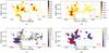 |
Fig. 4 Same as Fig. 3, but limited to 62 >VLSR> 40 km s-1. |
| In the text | |
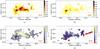 |
Fig. 5 Same as Fig. 3, but limited to 75 >VLSR> 62 km s-1. |
| In the text | |
|
Fig. 6 Map of the column-weighted volume density along the line of sight averaged over all velocities. The colors are greyed out where the S/N in the 110 − 111 line is less than ~ 7, with lower-signal regions being progressively more gray. |
| In the text | |
|
Fig. 7 Map of the column-weighted volume density along the line of sight, split into a) the 40−62 km s-1 component and b) the 62 to 75 km s-1 component. The similarity between the two figures is due to large line widths; the cut at 62 km s-1 is meant to highlight the low-density filament around ℓ = 49 and the clouds surrounding W51 Main. |
| In the text | |
|
Fig. 8 An example of the difference in models between a continuum source (red) and the CMB (green) as the background. The top plot shows the 110 − 111 line and the bottom shows the 211 − 212 line both with the continuum level set to zero in the plot. The residuals are shown offset above the spectra, with the dashed line indicating the zero-residual level. The grey shaded regions show the 1σ error bars on each pixel. The model with the CMB as the only background is able to reproduce the absorption line, while the model with the H ii region in the background cannot account for the depth of the 211 − 212 line. The reduced χ2/n for the models are 14.1 (red) and 2.8 (green), evaluated only over the pixels where the model is greater than the local rms. |
| In the text | |
|
Fig. 9 Top figure: a column density map fitted from the Herschel Hi-Gal data with two filament extraction regions superposed in cyan and purple. The purple extracted position-velocity diagram is shown in Fig. 10. Bottom figure: a position-velocity slice of the 68 km s-1 cloud, shown in cyan in the left figure, which includes an 8 μm-dark cloud and the interaction region with the W51C supernova remnant. (bottom figure, top panel) H2CO110 − 111 observed optical depth (bottom figure, middle panel) H2CO211 − 212 observed optical depth (bottom figure, bottom panel) 13CO 1−0 emission from the Galactic Ring Survey (GRS Jackson et al. 2006) with H2CO110 − 111 contours superposed. The weakness of the H2CO absorption on the right half of the cloud corroborates the geometry inferred from comparison of the 110 − 111 and 211 − 212 lines in Fig. 8. The 13CO emission without corresponding H2CO absorption at offset 0.2 degrees is primarily background material in the 51 km s-1 cloud (see Fig. 11. These figures were made using wcsaxes12 and pvextractor13). |
| In the text | |
|
Fig. 10 Position-velocity diagrams of filamentary structures to the north and south of W51 Main. The panels are H2CO110 − 111, 211 − 212, and 13CO 1−0 as in Fig. 9. The 50 km s-1 component at offset ~ 0.15 degrees (ℓ ≈ 49.47,b ≈ − 0.42) is in the background of the H ii region. The extracted region is identified in purple in Fig. 9; the left side of the position-velocity diagram corresponds to the b = −0.5 end of the region. |
| In the text | |
|
Fig. 11 A sketched diagram of the W51 region as viewed from the Galactic north pole, with the observer looking up the page from the bottom (i.e., W51C is the front-most labeled object along our line-of-sight). There are a few significant differences between this and Fig. 29 of Kang et al. (2010), particularly the relative geometry of the cloud and the H ii regions in W51 B. We also show a good deal more detail, revealing that there are H ii regions on both front and back of many clouds. The orange areas represent H ii regions and ionized gas (the W51 C SNR), while purple/blue/cyan regions show molecular clouds. The shapes of the clouds approximately reflect their shape on the sky, but these shapes are only intended as mnemonics to help associate this face-on view with the edge-on view of the real observations. Figure 12 shows the face-on view and can be compared side-by-side with this figure to get an approximate 3D view of the region. |
| In the text | |
|
Fig. 12 Labeled figures of the W51A and W51B regions, highlighting H ii regions and 8 μm-dark clouds. The colors are described in Fig. 1. These labels can be compared to Fig. 11 to associate labeled regions in the plane of the sky with their counterparts in the face-on view of our Galaxy. |
| In the text | |
|
Fig. 13 Dense gas mass fraction as a function of volume density threshold n(H2)cm-3. The y-axis shows the sum of 13CO pixels from the GRS cube with H2CO-derived density above the value shown on the x-axis divided by the total. Both values are computed over the velocity range 40 km s-1<vLSR< 75 km s-1. The solid line represents the fraction of 13CO emitting voxels above the mean measured H2CO density as described in Sect. 3.3. The blue shaded region shows the extent of plausible model fits at each density: effectively, this is the ~ 1σ error region. The vertical line at n = 104cm-3 indicates the approximate completeness limit. The horizontal line shows the fraction of 13CO flux in pixels that had corresponding detections at > 2σ in both the H2CO110 − 111 and 211 − 212 lines: it represents the upper limit of what could have been detected if, e.g., all H2CO detections were toward regions with n> 104cm-3. The failure to converge to a fraction f → fmax indicates that there are some real detections of low-density gas. |
| In the text | |
|
Fig. 14 Same as Fig. 13, but for two individual regions: W51 Main a), the region 49.4°<ℓ< 49.6°, − 0.5°<b< − 0.3°, and W51 B b) with 48.8°ℓ< 49.4° and − 0.5°<b< − 0.1°. Note that the y axes have different ranges. The area covered by the W51 B cutout is 6 × larger than the W51 A cutout, so its effect on Fig. 13 is greater. The total area covered in Fig. 13 includes some regions with no detected H2CO, which is why the peak fraction in that figure is lower. |
| In the text | |
|
Fig. 15 Contours of the dense gas mass fraction using two different thresholds overlaid on the integrated 13CO map. The regions with fraction f> 0.5 should be rapidly forming stars. The background image in both frames is the GRS 13CO image integrated over the range 40 km s-1<vlsr< 75 km s-1, masked to include only pixels with TB> 0.5 K. |
| In the text | |
|
Fig. 16 Top: a star-forming gas mass map, created by multiplying the dense gas fraction by the integrated 13CO mass surface density. The red symbols are Class I and flat-spectrum YSOs from Kang et al. (2009) with M< 10 M⊙ (×’s) and M> 10 M⊙ (circles). They are absent from the highest density regions. Bottom: a star formation rate surface density map computed from the MSX 21 cm and MIPS 24 μm (Price et al. 2001; Carey et al. 2009) data with a star formation rate computed using the Rieke et al. (2009) calibration (Kennicutt & Evans 2012). The contours show the star-forming gas surface density above a threshold n> 104cm-3 (red) and n> 105cm-3 (blue) at levels of [100,1000] M⊙ kpc-2. At low star-forming gas surface density, the star formation surface density is essentially anticorrelated with the gas surface density. The two converge at the highest surface densities and at the highest volume densities. |
| In the text | |
|
Fig. A.1 Comparison between the GBT and NRAO GBES (Langston et al. 2000) data. Top left: NRAO GBES 2 cm map (top right) GBT 2 cm map of the same region smoothed to about 8.9′. The colorbar applies to both figures, showing brightness temperature units in K. The red contours in both figures show the region observed by Green Bank; flux outside of those boundaries is extrapolated with the smoothing kernel. The green contours show the region where TB(GBT) >TB(GBES). Bottom: plot of the GBT vs. the GBES surface brightness measurements. The large red dots show the region within the red contours. |
| In the text | |
|
Fig. A.2 Comparison between the Arecibo and Urumqi 25 m (Sun et al. 2011b) data. Top left: Urumqi 6 cm map of the W51 region. Top right: Arecibo 6 cm map of the same region smoothed to the 9.5′ resolution of the Urumqi data set. The colorbar applies to both figures, showing brightness temperature units in K. The red contours in both figures show the region observed by Arecibo; flux outside of those boundaries is extrapolated with the smoothing kernel. Bottom: plot of the Arecibo vs. the Urumqi surface brightness measurements. The red dots show the region within the red contours. |
| In the text | |
|
Fig. A.3 5 GHz and 15 GHz continuum and RRL flux densities against one another; all units are in Jy. The dashed lines show the total least squares best fit line with the slope shown in the legend. Wherever the density of points is too high to display, the points have been replaced with a contour plot showing the density of data points. The upper-right panel shows a comparison of the continuum ratio to the RRL ratio. The dashed line in the upper-right plot has slope 1, and the dotted line has slope 0.6. |
| In the text | |
|
Fig. A.4 Ratio maps of the ionized gas in W51. a) Continuum ratio S15 GHz/S5 GHz. For α = −0.1, an optically thin free-free source, the ratio is 0.9, while for α = 2, an optically thick source, the ratio is 9. b) The ratio of the H77α peak to the H112α peak. c) The line-to-continuum ratio H112α/S5 GHz. d) The line-to-continuum ratio H77α/S15 GHz. |
| In the text | |
|
Fig. A.5 a) H112α electron temperature map showing |
| In the text | |
|
Fig. B.1 Spectrum extracted from G49.119-0.277 in a 55′′ radius aperture, showing a model in which the continuum is behind the 63 km s-1 component but in front of the 68 km s-1 component. The legend gives the fit parameters along with 1σ error bars. The parameters with no errors indicated (OPR, T, TBG) are assumed or independently measured values. |
| In the text | |
|
Fig. B.2 Fitted H110α (red) and H77α (black) spectra extracted from 55′′ apertures centered on G49.20-0.35 (top) and G49.1-0.4 (bottom). The best-fit Gaussian parameters are shown in the legends, with the lower legend corresponding to H77α. |
| In the text | |
|
Fig. B.3 a) Velocity of the peak H2CO110 − 111 signal (deepest absorption) at 1 km s-1 resolution. b) Velocity of the peak H110α emission as derived from Gaussian fits to each spectrum. |
| In the text | |
|
Fig. B.4 Maps of the fitted H2CO velocity components over the range 40 <vLSR< 66 km s-1 (left) and 66 <vLSR< 75 km s-1 (right). The regions that appear noisy have ambiguous multi-component decompositions. |
| In the text | |
|
Fig. B.5 A histogram of the abundances derived for each spatial pixel using the LVG grid fit. The abundance shown assumes a velocity gradient 1 km s-1pc-1. The overlaid fits show that 30% of the area of W51 is consistent with an abundance X(o - H2CO) = 10− 8.4 ± 0.5 and 70% with X(o - H2CO) = 10− 9.9 ± 0.6. |
| In the text | |
|
Fig. B.6 A large-scale color composite that highlights the W51 C supernova remnant as a white haze using 90 cm data from Brogan et al. (2013). The colors are the same as in Fig. 1: the blue, green, and red colors are WISE bands 1, 3, and 4 (3.4, 12, and 22 μm) respectively. The yellow-orange semitransparent layer is from the Bolocam 1.1 mm Galactic Plane Survey data (Aguirre et al. 2011; this paper). |
| In the text | |
Current usage metrics show cumulative count of Article Views (full-text article views including HTML views, PDF and ePub downloads, according to the available data) and Abstracts Views on Vision4Press platform.
Data correspond to usage on the plateform after 2015. The current usage metrics is available 48-96 hours after online publication and is updated daily on week days.
Initial download of the metrics may take a while.