| Issue |
A&A
Volume 571, November 2014
Planck 2013 results
|
|
|---|---|---|
| Article Number | A19 | |
| Number of page(s) | 23 | |
| Section | Cosmology (including clusters of galaxies) | |
| DOI | https://doi.org/10.1051/0004-6361/201321526 | |
| Published online | 29 October 2014 | |
Planck 2013 results. XIX. The integrated Sachs-Wolfe effect
1 APC, AstroParticule et
Cosmologie,Université Paris Diderot, CNRS/IN2P3, CEA/lrfu, Observatoire de
Paris, Sorbonne Paris Cité, 10 rue
Alice Domon et Léonie Duquet, 75205
Paris Cedex 13,
France
2 Aalto University Metsähovi Radio
Observatory, Metsähovintie
114, 02540
Kylmälä,
Finland
3 African Institute for Mathematical
Sciences, 6−8 Melrose Road,
Muizenberg, 7945
Cape Town, South
Africa
4 Agenzia Spaziale Italiana Science
Data Center, via del Politecnico snc, 00133
Roma,
Italy
5 Agenzia Spaziale Italiana, Viale
Liegi 26, 00198
Roma,
Italy
6 Astrophysics Group, Cavendish
Laboratory, University of Cambridge, J J Thomson Avenue, Cambridge
CB3 0HE,
UK
7 Astrophysics & Cosmology Research
Unit, School of Mathematics, Statistics & Computer Science, University of
KwaZulu-Natal, Westville Campus,
Private Bag X54001, 4000
Durban, South
Africa
8 CITA, University of
Toronto, 60 St. George St.,
Toronto, ON
M5S 3H8,
Canada
9 CNRS, IRAP, 9 Av. colonel Roche, BP 44346, 31028
Toulouse Cedex 4,
France
10 California Institute of
Technology, Pasadena,
California,
USA
11 Centre for Theoretical Cosmology,
DAMTP, University of Cambridge, Wilberforce Road, Cambridge
CB3 0WA,
UK
12 Centro de Estudios de Física del
Cosmos de Aragón (CEFCA), Plaza San Juan 1, planta 2, 44001
Teruel,
Spain
13 Computational Cosmology Center,
Lawrence Berkeley National Laboratory, Berkeley, California, USA
14 Consejo Superior de Investigaciones
Científicas (CSIC), 28006
Madrid,
Spain
15 DSM/Irfu/SPP,
CEA-Saclay, 91191
Gif-sur-Yvette Cedex,
France
16 DTU Space, National Space
Institute, Technical University of Denmark, Elektrovej 327, 2800
Kgs. Lyngby,
Denmark
17 Département de Physique Théorique,
Université de Genève, 24 quai E.
Ansermet, 1211
Genève 4,
Switzerland
18 Departamento de Física Fundamental,
Facultad de Ciencias, Universidad de Salamanca, 37008
Salamanca,
Spain
19 Departamento de Física, Universidad
de Oviedo, Avda. Calvo Sotelo
s/n, 33007
Oviedo,
Spain
20 Department of Astronomy and
Astrophysics, University of Toronto, 50 Saint George Street, Toronto, Ontario,
Canada
21 Department of Astrophysics/IMAPP,
Radboud University Nijmegen, PO Box
9010, 6500 GL
Nijmegen, The
Netherlands
22 Department of Electrical
Engineering and Computer Sciences, University of California,
Berkeley, California,
USA
23 Department of Physics &
Astronomy, University of British Columbia, 6224 Agricultural Road, Vancouver,
British Columbia,
Canada
24 Department of Physics and
Astronomy, Dana and David Dornsife College of Letter, Arts and Sciences, University of
Southern California, Los
Angeles, CA
90089,
USA
25 Department of Physics and
Astronomy, University College London, London
WC1E 6BT,
UK
26 Department of Physics, Carnegie
Mellon University, 5000 Forbes
Ave, Pittsburgh,
PA
15213,
USA
27 Department of Physics, Florida
State University, Keen Physics
Building, 77 Chieftan Way, Tallahassee, Florida, USA
28 Department of Physics, Gustaf
Hällströmin katu 2a, University of Helsinki, 00014
Helsinki,
Finland
29 Department of Physics, Princeton
University, Princeton, New
Jersey, USA
30 Department of Physics, University
of California, Berkeley, California, USA
31 Department of Physics, University
of California, One Shields
Avenue, Davis,
California,
USA
32 Department of Physics, University
of California, Santa
Barbara, California, USA
33 Department of Physics, University
of Illinois at Urbana- Champaign, 1110 West Green Street, Urbana, Illinois,
USA
34 Dipartimento di Fisica e Astronomia
G. Galilei, Università degli Studi di Padova, via Marzolo 8, 35131
Padova,
Italy
35 Dipartimento di Fisica e Scienze
della Terra, Università di Ferrara, via Saragat 1, 44122
Ferrara,
Italy
36 Dipartimento di Fisica, Università
La Sapienza, P.le A. Moro
2, 00185
Roma,
Italy
37 Dipartimento di Fisica, Università
degli Studi di Milano, via Celoria,
16, 20133
Milano,
Italy
38 Dipartimento di Fisica, Università
degli Studi di Trieste, via A.
Valerio 2, 34127
Trieste,
Italy
39 Dipartimento di Fisica, Università
di Roma Tor Vergata, via della
Ricerca Scientifica, 1, 00133
Roma,
Italy
40 Discovery Center, Niels Bohr
Institute, Blegdamsvej
17, 2100
Copenhagen,
Denmark
41 Dpto. Astrofísica, Universidad de
La Laguna (ULL), 38206 La
Laguna, Tenerife,
Spain
42 European SpaceAgency, ESAC, Planck
Science Office, Camino bajo del Castillo s/n, Urbanización Villafranca del Castillo,
28692 Villanueva de la Cañada, Madrid, Spain
43 European Space Agency, ESTEC,
Keplerlaan 1, 2201
AZ
Noordwijk, The
Netherlands
44 Haverford College Astronomy
Department, 370 Lancaster
Avenue, Haverford,
Pennsylvania,
USA
45 Helsinki Institute of Physics,
Gustaf Hällströmin katu 2, University of Helsinki, 00014
Helsinki,
Finland
46 INAF − Osservatorio Astrofisico di
Catania, via S. Sofia 78, 95123
Catania,
Italy
47 INAF − Osservatorio Astronomico di
Padova, Vicolo dell’Osservatorio 5, Padova, Italy
48 INAF − Osservatorio Astronomico di
Roma, via di Frascati 33, Monte Porzio Catone, 00040
Rome,
Italy
49 INAF − Osservatorio Astronomico di
Trieste, via G.B. Tiepolo 11, 34143
Trieste,
Italy
50 INAF Istituto di Radioastronomia,
via P. Gobetti 101, 40129
Bologna,
Italy
51 INAF/IASF Bologna, via Gobetti
101, 40129
Bologna,
Italy
52 INAF/IASF Milano, via E. Bassini
15, 20133
Milano,
Italy
53 INFN, Sezione di Bologna, via
Irnerio 46, 40126
Bologna,
Italy
54 INFN, Sezione di Roma 1, Università
di Roma Sapienza, Piazzale Aldo
Moro 2, 00185
Roma,
Italy
55 INFN/National Institute for Nuclear
Physics, via Valerio
2, 34127
Trieste,
Italy
56 IPAG: Institut de Planétologie et
d’Astrophysique de Grenoble, Université Joseph Fourier, Grenoble 1/CNRS-INSU, UMR
5274, 38041
Grenoble,
France
57 IUCAA, Post Bag 4, Ganeshkhind,
Pune University Campus, Pune
411 007,
India
58 Imperial College London,
Astrophysics group, Blackett Laboratory, Prince Consort Road, London, SW7
2AZ, UK
59 Infrared Processing and Analysis
Center, California Institute of Technology, Pasadena, CA
91125,
USA
60 Institut Néel, CNRS, Université
Joseph Fourier Grenoble I, 25 rue
des Martyrs, 38042
Grenoble,
France
61 Institut Universitaire de
France, 103 bd
Saint-Michel, 75005
Paris,
France
62 Institut d’Astrophysique Spatiale,
CNRS (UMR 8617) Université Paris-Sud 11, Bâtiment 121, 91405
Orsay,
France
63 Institut d’Astrophysique de Paris,
CNRS (UMR 7095), 98bis boulevard
Arago, 75014
Paris,
France
64 Institut de Ciències de l’Espai,
CSIC/IEEC, Facultat de Ciències, Campus UAB, Torre C5 par-2, 08193
Bellaterra,
Spain
65 Institute for Space
Sciences, 76900
Bucharest-Magurale,
Romania
66 Institute of Astronomy and
Astrophysics, Academia Sinica, Taipei, Taiwan
67 Institute of Astronomy, University
of Cambridge, Madingley
Road, Cambridge
CB3 0HA,
UK
68 Institute of Theoretical
Astrophysics, University of Oslo, Blindern, 0315
Oslo,
Norway
69 Instituto de Astrofísica de
Canarias, C/Vía Láctea s/n, 38200
La Laguna, Tenerife, Spain
70 Instituto de Física de Cantabria
(CSIC-Universidad de Cantabria), Avda. de los Castros s/n, 39005
Santander,
Spain
71 Jet Propulsion Laboratory,
California Institute of Technology, 4800 Oak Grove Drive, Pasadena, California, USA
72 Jodrell Bank Centre for
Astrophysics, Alan Turing Building, School of Physics and Astronomy, The University of
Manchester, Oxford
Road, Manchester,
M13 9PL,
UK
73 Kavli Institute for Cosmology
Cambridge, Madingley
Road, Cambridge,
CB3 0HA,
UK
74 LAL, Université Paris-Sud,
CNRS/IN2P3, 91898
Orsay,
France
75 LERMA, CNRS, Observatoire de Paris,
61 avenue de l’Observatoire, 75014
Paris,
France
76 Laboratoire AIM, IRFU/Service
d’Astrophysique − CEA/DSM − CNRS − Université Paris Diderot, Bât. 709,
CEA-Saclay, 91191
Gif-sur-Yvette Cedex,
France
77 Laboratoire Traitement et
Communication de l’Information, CNRS (UMR 5141) and Télécom ParisTech,
46 rue Barrault, 75634
Paris Cedex 13,
France
78 Laboratoire de Physique Subatomique
et de Cosmologie, Université Joseph Fourier Grenoble I, CNRS/IN2P3, Institut National
Polytechnique de Grenoble, 53 rue
des Martyrs, 38026
Grenoble Cedex,
France
79 Laboratoire de Physique Théorique,
Université Paris-Sud 11 & CNRS, Bâtiment 210, 91405
Orsay,
France
80 Lawrence Berkeley National
Laboratory, Berkeley,
California,
USA
81 Max-Planck-Institut für
Astrophysik, Karl-Schwarzschild-Str. 1, 85741
Garching,
Germany
82 McGill Physics, Ernest Rutherford
Physics Building, McGill University, 3600 rue University, Montréal, QC, H3A 2T8,
Canada
83 MilliLab, VTT Technical Research
Centre of Finland, Tietotie 3, 02044
Espoo,
Finland
84 Niels Bohr Institute,
Blegdamsvej 17, Copenhagen,
Denmark
85 Observational Cosmology, Mail
Stop367-17, California Institute of Technology, Pasadena, CA
91125,
USA
86 Optical Science Laboratory,
University College London, Gower
Street, London,
UK
87 SB-ITP-LPPC, EPFL,
1015
Lausanne,
Switzerland
88 SISSA, Astrophysics Sector, via
Bonomea 265, 34136
Trieste,
Italy
89 School of Physics and Astronomy,
Cardiff University, Queens
Buildings, The Parade, Cardiff, CF24
3AA, UK
90 School of Physics and Astronomy,
University of Nottingham, Nottingham
NG7 2RD,
UK
91 Space Research Institute (IKI),
Russian Academy of Sciences, Profsoyuznaya Str, 84/32, Moscow
117997,
Russia
92 Space Sciences Laboratory,
University of California, Berkeley, California, USA
93 Special Astrophysical Observatory,
Russian Academy of Sciences, Nizhnij Arkhyz, Zelenchukskiy region, 369167
Karachai-Cherkessian Republic,
Russia
94 Stanford University,
Dept of Physics, Varian Physics Bldg, 382 via
Pueblo Mall, Stanford, California, USA
95 Sub-Department of Astrophysics,
University of Oxford, Keble
Road, Oxford
OX1 3RH,
UK
96 Theory Division, PH-TH,
CERN, 1211
Geneva 23,
Switzerland
97 UPMC Univ. Paris 06, UMR
7095, 98bis boulevard
Arago, 75014
Paris,
France
98 Universität Heidelberg, Institut
für Theoretische Astrophysik, Philosophenweg 12, 69120
Heidelberg,
Germany
99 Université de
Toulouse, UPS-OMP,
IRAP, 31028
Toulouse Cedex 4,
France
100 University Observatory, Ludwig
Maximilian University of Munich, Scheinerstrasse 1, 81679
Munich,
Germany
101 University of Granada,
Departamento de Física Teórica y del Cosmos, Facultad de Ciencias,
18071
Granada,
Spain
102 Warsaw University
Observatory, Aleje Ujazdowskie
4, 00-478
Warszawa,
Poland
Received:
21
March
2013
Accepted:
25
November
2013
Based on cosmic microwave background (CMB) maps from the 2013 Planck Mission data release, this paper presents the detection of the integrated Sachs-Wolfe (ISW) effect, that is, the correlation between the CMB and large-scale evolving gravitational potentials. The significance of detection ranges from 2 to 4σ, depending on which method is used. We investigated three separate approaches, which essentially cover all previous studies, and also break new ground. (i) We correlated the CMB with the Planck reconstructed gravitational lensing potential (for the first time). This detection was made using the lensing-induced bispectrum between the low-ℓ and high-ℓ temperature anisotropies; the correlation between lensing and the ISW effect has a significance close to 2.5σ. (ii) We cross-correlated with tracers of large-scale structure, which yielded a significance of about 3σ, based on a combination of radio (NVSS) and optical (SDSS) data. (iii) We used aperture photometry on stacked CMB fields at the locations of known large-scale structures, which yielded and confirms a 4σ signal, over a broader spectral range, when using a previously explored catalogue, but shows strong discrepancies in amplitude and scale when compared with expectations. More recent catalogues give more moderate results that range from negligible to 2.5σ at most, but have a more consistent scale and amplitude, the latter being still slightly higher than what is expected from numerical simulations within ΛCMD. Where they can be compared, these measurements are compatible with previous work using data from WMAP, where these scales have been mapped to the limits of cosmic variance. Planck’s broader frequency coverage allows for better foreground cleaning and confirms that the signal is achromatic, which makes it preferable for ISW detection. As a final step we used tracers of large-scale structure to filter the CMB data, from which we present maps of the ISW temperature perturbation. These results provide complementary and independent evidence for the existence of a dark energy component that governs the currently accelerated expansion of the Universe.
Key words: cosmic background radiation / large-scale structure of Universe / dark energy / galaxies: clusters: general / methods: data analysis
© ESO, 2014
1. Introduction
This paper, one of a set associated with the 2013 data release from the Planck1 mission (Planck Collaboration I 2014), presents the first results on the integrated Sachs-Wolfe (ISW) effect using Planck data. The ISW effect (Sachs & Wolfe 1967; Rees & Sciama 1968; Martinez-Gonzalez et al. 1990; Hu & Sugiyama 1994) is a secondary anisotropy in the cosmic microwave background (CMB), caused by the interaction of CMB photons with the time-evolving potentials from large-scale structure (LSS). Photons follow a geodesic that is weakly perturbed by the Newtonian gravitational potential, Φ, and experience a fractional shift in their temperature given by  (1)where the integral is expressed in terms of the conformal time η, defined differentially by dη/ da = 1 / (a2H(a)), with H(a) the Hubble function and a the scale factor. The integration limits here extend from the recombination time (η∗) to the present time (η0).
The sensitivity of the ISW effect to gravitational potentials (that can extend over Gpc scales) causes the power of the ISW to be concentrated on the largest scales. The largest scales for the CMB have been mapped out by the Wilkinson Microwave Anisotropy Probe (WMAP) to the statistical limit of cosmic variance. Some systematics (like foreground removal) can have an impact on the reconstruction of the CMB especially at the largest scales where our Galaxy can introduce significant residuals on the reconstructed CMB map. The superior sensitivity of Planck together with its better angular resolution and wider frequency coverage allows for a better understanding (and hence removal) of Galactic and extagalactic foregrounds, which reduces the possible negative impact of these residuals. Planck allows us to improve on previous measurements through a better systematic control, an improved removal of foregrounds (which permits us to explore the achromatic nature of the ISW signal on a wider frequency range), and a better understanding of systematics affecting tracer catalogues.
For cosmological models where Ωm = 1, gravitational potentials remain constant during linear structure formation, and the ISW signal is negligible (to first order, although second-order nonlinear ISW is always expected around smaller over- and underdense regions). In the presence of dark energy, decaying potentials due to the accelerated expansion rate result in a net ISW effect that is positive when the CMB photons cross overdense regions and negative when the CMB photons cross underdense regions. Therefore, the ISW effect is an indicator of either nonzero curvature (Kamionkowski & Spergel 1994)2, any form of dark energy, such as a cosmological constant Λ (Crittenden & Turok 1996), modified gravity (Hu 2002), or a combination of these possibilities. By measuring the rate at which gravitational potentials in the LSS decay (up to a redshift of about 2), the ISW effect can be used as an independent probe of cosmology and provides complementary and independent evidence for dark energy.
Detection of the ISW effect was first made possible with all-sky CMB maps from WMAP. Based on these data, many works can be found in the literature where the authors aim at making, and subsequectly improving, the measurement of the ISW effect through correlations with tracer catalogues: 2MASS (an infrared catalogue out to low redshifts around 0.1, Afshordi et al. 2004; Rassat et al. 2007; Francis & Peacock 2010b; Dupé et al. 2011), HEAO (an X-ray survey at low redshift, with the first positive claim of detection, Boughn & Crittenden 2004), Sloan Digital Sky Survey (SDSS, an optical survey at intermediate redshifts, Fosalba et al. 2003; Scranton et al. 2003; Fosalba & Gaztañaga 2004; Padmanabhan et al. 2005; Cabré et al. 2006; Giannantonio et al. 2006; Granett et al. 2009; Xia 2009; Bielby et al. 2010; López-Corredoira et al. 2010; Sawangwit et al. 2010), the NRAO VLA Sky Survey (NVSS, a radio catalogue with high-redshift sources, Boughn & Crittenden 2005; Vielva et al. 2006; Pietrobon et al. 2006a; McEwen et al. 2007; Raccanelli et al. 2008; Hernández-Monteagudo 2010; Massardi et al. 2010; Schiavon et al. 2012), and combined measurements with multiple tracers (Nolta et al. 2004; Ho et al. 2008; Corasaniti et al. 2005; Gaztañaga et al. 2006; Giannantonio et al. 2008, 2012). The significance of the ISW detections that can be found in the literature range between 0.9σ and 4.7σ. There are a number of peculiarities related to some of the detection claims, as noted by Hernández-Monteagudo (2010) and López-Corredoira et al. (2010). They both found lower significance levels than some previous studies and pointed out the absence of the signal at low multipoles where the ISW effect should be most prominent and the presence of point source emission on small scales for radio surveys.
The main result that is obtained from an ISW detection is a constraint on the cosmological constant (or dark energy), ΩΛ. The general consensus from the variety of ISW analyses is for a value of ΩΛ ≃ 0.75 with an error of about 20%, which provides independent evidence for the existence of dark energy (Fosalba et al. 2003; Fosalba & Gaztañaga 2004; Nolta et al. 2004; Corasaniti et al. 2005; Padmanabhan et al. 2005; Cabré et al. 2006; Giannantonio et al. 2006; Pietrobon et al. 2006b; Rassat et al. 2007; Vielva et al. 2006; McEwen et al. 2007; Ho et al. 2008; Schiavon et al. 2012). All tests on spatial flatness found an upper limit for ΩK of a few percent (Nolta et al. 2004; Gaztañaga et al. 2006; Ho et al. 2008; Li & Xia 2010). Using a prior on spatial flatness, the dark energy equation of state parameter, w, was found to be close to −1 (Giannantonio et al. 2006; Vielva et al. 2006; Ho et al. 2008), and a strong time evolution has been excluded (Giannantonio et al. 2008; Li & Xia 2010).
The ISW effect is achromatic, that is, it conserves the Planck spectrum of the CMB. Nevertheless, it can be separated from other CMB fluctuations through cross-correlations with catalogues that trace the LSS gravitational potentials (see for instance Crittenden & Turok 1996). This cross-correlation can be studied in different ways: through angular cross-correlations in real space between the CMB and the catalogues tat trace the LSS; through the corresponding angular cross-power spectrum of the Fourier-transformed maps; or through the covariance of wavelet-filtered maps as a function of wavelet scale. The studies using WMAP data mentioned above follow this survey cross-correlation techique.
An alternative approach, similar to the angular cross-correlation in real space, consists of stacking CMB fields centred on known supersclusters or supervoids (Granett et al. 2008a,b; Pápai & Szapudi 2010). The advantage of this technique is that it allows for a detailed study of the profile of the CMB fluctuations caused by this secondary anisotropy.
A novel and powerful approach takes advantage of the fact that the same potentials that cause CMB photons to gain or lose energy along their path (ISW) create lensing distortions that can be directly measured from the CMB map (e.g., Hu & Okamoto 2002). The interplay between weak gravitational lensing and the ISW effect causes a non-Gaussian contribution to the CMB, which can be measured through the lensing-induced bispectrum between small and large angular scales. The measurement of the lensing potential requires a large number of modes that could not be measured before the arrival of Planck data.
This paper presents new measurements of the ISW effect carried out with Planck. Even although our detections are not in every case as strong as some previously claimed significance levels, we believe that our results are an improvement over earlier studies. This is because we can use the additional power enabled by the frequency coverage and sensitivity of Planck. To establish this we carried out a comprehensive study of all the main approaches that have previously been taken to estimate the ISW signal. We also present new results in relation to the non-Gaussian structure induced by the ISW effect.
The paper is organized as follows: in Sect. 2 we describe the data used in this work (both for the CMB and large-scale structure). The first-ever results of estimating the lensing-induced bispectrum are presented in Sect. 3. Cross-correlations with external surveys are investigated in Sect. 4, and in Sect. 5 we present the results for the stacking analysis on the temperature maps, and aperture photometry on superclusters and supervoids. The recovery of the ISW all-sky map is described in Sect. 6. Finally, we discuss our main results and their cosmological implications in Sect. 7.
2. Data description
In this section we describe the different data sets. This includes Planck data (the CMB temperature and lensing potential maps, see Planck Collaboration I 2014; Planck Collaboration II 2014; Planck Collaboration VI 2014; Planck Collaboration XII 2014; Planck Collaboration XVII 2014, for details), and external data sets (large-scale structure tracers) used in determining the ISW: the radio NVSS catalogue, optical luminous galaxies (CMASS/LOWZ) and the main galaxy sample from the Sloan Digital Sky Survey (SDSS), and several superstructure catalogues.
2.1. Planck data
Planck data and products are described in the following sections, in particular the foreground-cleaned CMB maps produced by the Planck component separation pipelines, and related products, such as dedicated component-separated frequency maps (Planck Collaboration XII 2014), and the Planck lensing map (Planck Collaboration XVII 2014).
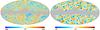 |
Fig. 1 Left: one of the CMB maps, constructed using SEVEM (given at Nside = 64). Other Planck CMB maps are Commander-Ruler, NILC and SMICA, in addition to clean SEVEM maps from 44 to 353 GHz. Right: Planck lensing map, optimally filtered to perform the ISW–lensing cross-correlation (given at Nside = 1024). See Planck Collaboration XII (2014) and Planck Collaboration XVII (2014) for a detailed description of these maps. |
2.1.1. CMB maps
We used the Planck foreground-cleaned CMB maps provided by the data processing centres (as described in the Planck component separation paper, Planck Collaboration XII 2014). In particular, to test their reliability, some of the results are presented for different cleaned CMB maps, which were constructed using four different component separation techniques: Commander-Ruler (C-R, which uses physical parametrization), NILC (an internal linear combination technique), SEVEM (a template-fitting method), and SMICA (which uses spectral matching). Since the contribution of the ISW signal is only significant on large scales, we used low-resolution maps, with HEALPix Górski et al. (2005) parameter Nside = 64 and a pixel size of about 55 arcmin for most of the analyses. One exception is the study of the correlation between the ISW and lensing signals, which requires the use of full-resolution maps (Nside = 2048, pixel size of 1.7 arcmin). The maps were degraded directly from the original full resolution to the corresponding Nside.
In addition, foreground-cleaned maps per frequency (from 44 to 353 GHz) at resolution Nside = 512 were used for the stacking analysis presented in Sect. 5. These maps were constructed by subtracting a linear combination of internal templates using SEVEM (for a detailed description of the method see the SEVEM appendix of Planck Collaboration XII 2014). As an example, the SEVEM CMB map is shown in Fig. 1 (left panel).
Finally, to minimize the foreground contamination in the maps, we used the official mask described in Planck Collaboration XII (2014), which excludes regions with stronger Galactic and point-source contamination (the U73 mask). This mask is given at the full Planck resolution and is downgraded to the required levels. The downgrading procedure consists of the following steps: the mask (originally a map with zero and one values) is convolved with a Gaussian beam of FWHM three times the characteristic pixel size of the final Nside resolution; this convolved map is then degraded to the required Nside, and, subsequently, a threshold of 0.75 is imposed (i.e., pixels with a value higher than this threshold are set to one, whereas the rest are set to zero).
2.1.2. Lensing potential map
Weak gravitational lensing distorts the CMB temperature anisotropy pattern. This effect is sensitive to the projected matter distribution in the large-scale structure at high redshifts, where structure growth is linear and the statistics are close to Gaussian. Weak lensing causes correlations between different multipoles, which are proportional to the lensing deflection field. These correlations can be exploited to reconstruct the density field and to measure its statistical properties (Hu & Okamoto 2002; Okamoto & Hu 2003). The lensing effect in the CMB can be estimated by this homogeneity breaking, and in this way, individual modes of the lensing potential at multipoles ℓ < 100 can be reconstructed with a significance of about 0.5σ, which shows that a statistical treatment is necessary. Nevertheless, the overall effect of the lensing is measured to better than 25σ (Planck Collaboration XVII 2014). The additional lensing effect in the temperature power spectrum is detectable with a significance of about 10σ (Planck Collaboration XV 2014).
With Planck data, we aim at detecting a correlation between the ISW effect and the lensing potential, where the latter is a tracer of the large-scale structure at high redshift. This correlation is restricted to 9σ, even in the ideal case, limited by cosmic variance and the weakness of the ISW effect in comparison to the primary CMB (Lewis et al. 2011). The data products used in this study are the Planck lensing potential reconstruction and specific lensing maps obtained from the component separation pipelines. The lensing potential is available as part of the first Planck data release. Its detailed development is described in the Planck lensing paper (Planck Collaboration XVII 2014). In Fig. 1 we reproduce (right panel) an optimally filtered version of the Planck lensing map, suitable for the ISW-lensing cross-correlation.
In addition to a direct correlation between the CMB sky and the reconstructed lensing map, we measured the bispectrum generated by weak lensing by applying a range of estimators: the KSW-bispectrum estimator, bispectra binned in multipole intervals and a modal decomposition of the bispectrum. This meassurement is made possible for the first time thanks to the Planck data. In addition, we used information from the lensing field as a tracer for an ISW map reconstruction at high redshift (see Sect. 6).
2.2. External data sets
As described in the introduction, the achromatic nature of the ISW effect requires a tracer of the gravitational potentials from the large-scale structure, so that by cross-correlating the CMB temperature map with that tracer distribution the fluctuations generated by the ISW effect are singled out. The prerequisites for a tracer catalogue to be used in ISW studies are a large survey volume, well-understood biasing properties, and low or at least well-modelled systematics. The radio NVSS catalogue and the optical luminous galaxies (SDSS-CMASS/LOWZ) and main photometric galaxy sample (SDSS-MphG) catalogues possess these qualities. Table 7 summarizes some basic properties of these catalogues. In addition, the redshift distributions of these catalogues are shown in Fig. 2. Note that NVSS presents the widest redshift coverage. The SDSS-CMASS/LOWZ sample peaks at about z ≈ 0.5, whereas the SDSS-MphG sample peaks at about z ≈ 0.3.
Figure 3 shows the all-sky density projection for these maps, where the grey area indicates regions not observed by these surveys (or that were discarded because they were contaminated or had a low galaxy number density, see next subsections for details). In Fig. 4 we give the angular power spectra (blue points) of the surveys (corrected for with a procedure similar to MASTER, e.g., Hivon et al. 2002), and the theoretical spectra (black lines) and their 1σ error bars (grey areas), estimated from the MASTER approach as well.
Main characteristics of the galaxy catalogues used as tracers of the gravitational potential.
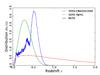 |
Fig. 2 Redshift distributions of the different surveys used as LSS tracers, to be correlated with the Planck CMB maps. To facilitate comparison, these distributions have been normalized to unity. |
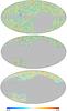 |
Fig. 3 Density contrast maps obtained from the galaxy catalogues at Nside = 64. From top to bottom: NVSS, SDSS-CMASS/LOWZ and SDSS-MphG. |
In addition to the cross-correlation between CMB and LSS tracers (Sect. 4), we present results from a different methodology in Sect. 5, where we used catalogues of superstructures to study the ISW through stacking of the CMB fluctuations on the positions of these superstructures. The relevant catalogues are described in Sect. 2.2.4.
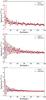 |
Fig. 4 Angular power spectra from the maps in Fig. 3. From top to bottom: NVSS, SDSS-CMASS/LOWZ, and SDSS-MphG. The observed spectra are the red points, while the theoretical models are represented by the black lines (the grey areas correspond to the sampling variance). |
2.2.1. NVSS radio catalogues
Luminous active galactic nuclei (hereafter AGN) are known to be powerful radio sources that are visible out to high redshifts. These sources are hence able to probe the cosmic density field during the entire redshift range from matter domination to accelerated expansion due to dark energy. If AGN are fair tracers of the underlying density field, these sources should likewise probe the spatial distribution of the large-scale potential wells that decay at late times after the accelerated expansion sets in and generates the ISW effect.
We focused on a single radio survey that has the level of sensitivity and sky coverage required for ISW studies, namely the NRAO VLA Sky Survey (hereafter NVSS, Condon et al. 1998). This survey was conducted using the Very Large Array (VLA) at 1.4 GHz, and covers up to an equatorial latitude of bE = − 40deg, with an average noise level of 0.45 mJy beam-1. It results in roughly 1.4 × 10⁶ sources above a flux threshold of 2.5 mJy. Figure 3 displays the number density map computed from the NVSS survey (top panel). The AGN population is known to be dominant in radio catalogues at 1.4 GHz in the high flux density regime. Condon et al. (1998) showed that at this frequency, star-forming galaxies (SFGs) contribute about 30% of the total number of weighted source counts above 1 mJy, but their presence decreases rapidly as higher flux thresholds are adopted. The NVSS SFGs are nearby sources (z< 0.01), and hence may distort the ability of our radio template to probe the intermediate and high-redshift density field.
We next address the systematic effects in the NVSS survey. Two different antenna configurations were used while conducting the NVSS survey: the D-configuration (for bE ∈ [ − 10deg, 78deg ]), and the DnC-configuration for large zenith angles (bE< − 10deg,bE> 78deg). This change in the antenna configuration is known to introduce changes in the source number density above 2.5 mJy, as first pointed out by Blake & Wall (2002). The NVSS map at 2.5 mJy was corrected for this declination systematic using the following procedure: the sky was divided into equatorial strips and the mean number of sources in each strip was re-normalized to the full sky mean (see e.g., Vielva et al. 2006). With this procedure the average number of sources in the NVSS map is the same as before the correction, and hence the shot noise level does not change. The number of strips into which the map was divided is 70, but the results are independent of this choice.
Regarding the galaxy bias, we adopted the Gaussian bias-evolution model of Xia et al. (2011). If n(M,z) is the halo mass function and b(M,z) is the bias of halos with comoving mass M, then the bias of the survey is given by a mass-weighted integral,  (2)This model depends on the minimum mass Mmin of halos present in the survey. The upper limit in the mass is taken to be infinity because the effect of the high-mass end on the bias is negligible. Marcos-Caballero et al. (2013) proposed a theoretical model for the NVSS angular power spectrum, which also takes into account the information of the redshift distribution given by CENSORS data (Brookes et al. 2008). The redshift distribution is parametrized by
  (3)where z0 = 0.33 and α = 0.37. The parameter n0 is a constant to obtain a distribution normalized to unity. This function is represented in Fig. 2. The bias follows the prescription of Eq. (2), with Mmin equal to 1012.67M⊙, where the Sheth-Tormen (Sheth & Tormen 1999) mass function is adopted. Hereafter this model is our fiducial model for NVSS.
2.2.2. SDSS luminous galaxies
For this analysis we used the photometric luminous galaxy (LG) catalogue from the Baryonic Oscillation Spectroscopic Survey (BOSS) of the SDSS III. The data used consist of two sub-samples: CMASS and LOWZ. The two samples were combined to form a unique LG map (see Fig. 3, second panel). Hereafter, these samples are referred to as SDSS-CMASS, SDSS-LOWZ, and SDSS-CMASS/LOWZ for the combination.
SDSS-CMASS
We used the BOSS targets to obtain an approximately constant stellar mass; this is known as the photometric CMASS sample. This sample is mostly contained in the redshift range z = 0.4 − 0.7, with a galaxy number density close to 110 deg-2, and was selected after applying the colour cuts explained in Ross et al. (2011).
While this colour selection yields a catalogue of about 1 600 000 galaxies, more cuts were needed to be applied to account for dust extinction (based on the maps by Schlegel et al. 1998 with the criterion E(B − V) < 0.08), for seeing in the r band (required to be <2.0′′), and for the presence of bright stars, similar to Ho et al. (2012). Finally, we neglected all pixels with a mask value inferred from the footprint below 0.9 on a HEALPix map of resolution Nside = 64. This procedure left about one million sources 10 500 deg2. Photometric redshifts of this sample were calibrated using a selection of about 100 000 BOSS spectra as a training sample for the photometric catalogue. These LGs are among the most luminous galaxies in the Universe and therefore allow for a good sampling of the largest scales. Given the large number of the sources included in the sample, shot-noise does not dominate clustering errors. According to Ross et al. (2011), about 3.7% of these objects are either stars or quasars, which necessitates additional corrections, as explained at the end of this section.
SDSS-LOWZ
The photometric LOWZ sample is one of the two galaxy samples targeted by the BOSS of Sloan III. It selectd luminous, highly biased, mostly red galaxies, placed at an average redshift of ⟨ z ⟩ ~ 0.3 and below the redshifts of the CMASS sample (z< 0.4). Our selection criteria in terms of the Sloan five-model magnitudes ugriz followed those given in Sect. 2 of Parejko et al. (2013). With a total number of sources close to 600 000, this photometric sample contains a higher number density of galaxies in the southern part of the footprint than in the northern one (by more than 3%), which seems to be at odds with ΛCDM predictions. However, most of this effect vanishes after subtracting the dipole in the effective area under analysis in such a way that the low ℓ range of the auto power spectrum is consistent with a ΛCDM model and a constant bias b ≃ 2 (Hernández-Monteagudo et al. 2013).
The SDSS-CMASS and SDSS-LOWZ samples were also corrected for scaling introduced by possible systematics such as stars, mask value, seeing, sky emission, airmass, and dust extinction. Following exactly the same procedure as in Hernández-Monteagudo et al. (2013), we found that both LG samples were contaminated by stars in the sense that the galaxy number density decreased in areas with higher star density, since the latter tend to “blind” galaxy detection algorithms.
2.2.3. Main photometric SDSS galaxy sample
We used a sample of photometrically selected galaxies from the SDSS-DR8 catalogue, which covers a total sky area of 14 555 deg2 (Aihara et al. 2011). The total number of objects labelled as galaxies in this data release is 208 million. From this catalogue, and following Cabré et al. (2006), we defined a subsample by selecting only objects within the range 18 <r< 21, where this r-band model magnitude corrected for extinction. Following Giannantonio et al. (2008), we also restricted our subsample to objects with redshifts 0.1 <z< 0.9 and with measured redshift errors such that σz< 0.5z. We relied on the photometric redshift estimates of the SDSS photo-z primary galaxy table, which were obtained through a kd-tree nearest-neighbour technique by fitting the spectroscopic objects observed with similar colour and inclination angle. The total number of galaxies in our final sample is about 42 million, with redshifts distributed around a median value of about 0.35, as shown in Fig. 2. To avoid possible errors introduced by singularities in the photometric redshift estimates, instead of using the real observed redshift distribution in our analysis, we resorted to the analytical function  (4)which was fitted to the data with parameters m = 1.5, β = 2.3 and z0 = 0.34, which are identical to those found by Giannantonio et al. (2012). For the galactic bias we used the value b = 1.2, which was found by Giannantonio et al. (2012) by fitting the ΛCDM prediction to the observed auto-correlation function of the galaxies, and we adopted the mask proposed by them.
2.2.4. SDSS superstructures
Granett et al. (2008b) produced a sample3 of 50 superclusters and 50 supervoids identified from the luminous red galaxies (LRGs) in the SDSS (sixth data release, DR6, Adelman-McCarthy et al. 2008), which covers an area of 7500 deg2 on the sky. They used publicly available algorithms, based on the Voronoi tessellation, to find 2836 superclusters (using VOBOZ, VOronoi BOund Zones, Neyrinck et al. 2005) and 631 supervoids (using ZOBOV, ZOnes Bordering On Voidness, Neyrinck 2008) above a 2σ significance level (defined as the probability of obtaining, in a uniform Poisson point sample, the same density contrasts as those of clusters and voids). The 50 superclusters and 50 supervoids they published in their catalogue correspond to density contrasts of about 3σ and 3.3σ, respectively. They span a redshift range of 0.4 <z< 0.75, with a median of around 0.5, and inhabit a volume of around 5 h-3 Gpc3. These superstructures can potentially produce measurable ISW signals, as suggested in Granett et al. (2008a,b). For each structure, the catalogue provides the position on the sky of the centre, the mean and maximum angular distance between the galaxies in the structure and its centre, the physical volume and three different measures of the density contrast (calculated from all its Voronoi cells, from only its over- or underdense cells, and from only its most over- or underdense cells). We concentrated here on using the supervoid catalogue by Granett et al. (2008b) because it can be compared with two other, more recent catalogues of voids.
The second catalogue of cosmic voids that we considered here was published by Pan et al. (2012)4. It has been built from the seventh data release (DR7) of the SDSS. Using the VoidFinder algorithm (Hoyle & Vogeley 2002), the authors identified 1055 voids with redshifts lower than z = 0.1. Each void is listed with its position on the sky, its physical radius (defined as the radius of the largest sphere enclosing the void), an effective radius defined as the radius of a sphere of the same volume, its physical distance to us, its volume, and its mean density contrast. The filling factor of the voids in the sample volume is 62%. The largest void is just over 47 Mpc in effective radius, while the median effective radius of the void sample is about 25 Mpc. Some of the voids are both very close to us and relatively large (larger than 30 Mpc in radius), which results in large angular sizes of up to 15deg.
The third void catalogue that we used has been released by Sutter et al. (2012) and was also made publicly available5. Note that it is being updated regularly, and the results reported here are based on the version of 21 February 2013 of the catalogue. Using their own modified version of ZOBOV, these authors identified 1495 voids distributed across the 0–0.44 redshift range. They subdivided their catalogue into six subsamples: dim1, dim2, bright1, and bright2, constructed from the main SDSS, and lrgdim and lrgbright built from the SDSS LRG sample. For each void, the information provided includes the position of the centre, the redshift, the volume, the effective radius, and the density contrast.
3. ISW-lensing bispectrum
There is an interesting interplay between gravitational lensing of the CMB and the ISW effect, which manifests itself as a non-Gaussian feature. CMB-lensing can be described by a convolution of the CMB-temperature map T with the weak-lensing potential φ (e.g., Lewis & Challinor 2006), 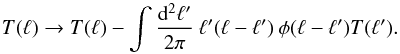 (5)The CMB lensing can be measured by a direct estimate of the CMB bispectrum, because the bispectrum acquires first-order terms proportional to the product of two power spectra
  , where
  is the lensed temperature power spectrum and
  is the temperature-potential cross-power spectrum. The potential field φ and the temperature field T are correlated, because φ, which deflects the CMB photons, also gives rise to the ISW effect in T (Hu & Okamoto 2002; Seljak & Zaldarriaga 1999; Verde & Spergel 2002; Giovi et al. 2003). This secondary bispectrum contains new information about the cosmological redshift, because it is generated mainly at redshifts higher than unity, and biases measurements of the primordial bispectrum. The term correlates the CMB temperature on small scales with the lensing potential on large scales, and causes the bispectrum to assume large amplitudes in the squeezed-triangles configuration (see e.g., Goldberg & Spergel 1999; Seljak & Zaldarriaga 1999; Hu 2000; Giovi et al. 2003; Okamoto & Hu 2003; Giovi & Baccigalupi 2005; Lewis & Challinor 2006; Serra & Cooray 2008; Mangilli & Verde 2009; Hanson et al. 2009, 2010; Smith & Zaldarriaga 2011; Lewis et al. 2011).
Owing to the rotational invariance of the sky, the CMB angular bispectrum ⟨ aℓ1m1aℓ2m2aℓ3m3 ⟩ can be factorized as follows: 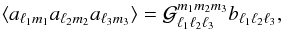 (6)where
  is the Gaunt-integral and bℓ1ℓ2ℓ3 is the so-called reduced bispectrum. When the bispectral signal on the sky is generated by the ISW-lensing effect,
 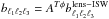 , where ATφ parametrizes the amplitude of the effect and
 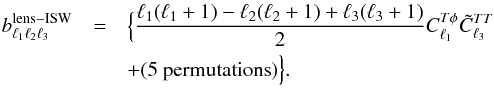 (7)A more general expression for intensity and polarization can be found in Lewis et al. (2011). Estimating the bispectrum then yields a measurement of ATφ.
We can also define an alternative rotationally invariant reduced bispectrum Bℓ1ℓ2ℓ3 as 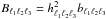 , where
 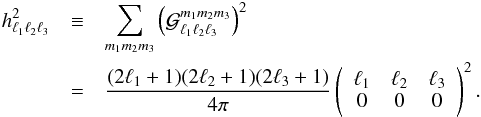 (8)The interest in Bℓ1ℓ2ℓ3 is that it can be directly estimated from the observed map using the expression
 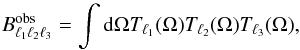 (9)where the filtered maps Tℓ(Ω) are defined as
  (10)By basically combining the single-ℓ estimates Bobs/Blens − ISW for ATφ using inverse variance weighting, the ISW-lensing bispectrum estimator can be written as (see Planck Collaboration XXIV 2014, for more details)
  (11)where the inner product is defined by
  (12)Here, Blin is a linear correction that has zero average but reduces the variance of the estimator in the presence of anisotropic noise and a mask. Furthermore,
  , with g being a simple permutation factor (g = 6 when all ℓ are equal, g = 2 when two ℓ are equal and g = 1 otherwise). As in all expressions in this section, we implicitly took the beam and noise of the experiment into accout, which means that Cℓ should actually be
  , with bℓ the beam transfer function and Nℓ the noise power spectrum.
In Eq. (11) we have also used the fact that, as discussed in detail in Planck Collaboration XXIV (2014), the full inverse covariance weighting can be replaced by a diagonal covariance term, (C-1a)ℓm → aℓm/Cℓ, without loss of optimality, if the masked regions of the map are filled in with a simple diffusive inpainting scheme.
The normalization of the lensing-ISW estimator in the denominator of Eq. (11) can be replaced by (see e.g. Lewis et al. 2011)  (13)where
  parameterizes the deviation from the Cauchy-Schwarz relation and Fℓ is given in terms of the ISW-lensing bispectrum (see for example Lewis et al. 2011). The first term in Eq. (13) corresponds to the Fisher errors assuming Gaussian aℓm. However, contrary to the null hypothesis that is assumed, for example, in the primordial bispectra (Gaussianity), there is an actual non-Gaussian signal already present in the ISW-lensing bispectrum. This guarantees a larger variance for the estimators than are included in the additional terms present in the previous equations.
An important issue is the impact of the ISW-lensing bispectrum on estimates of the primordial non-Gaussianity. Assuming weak levels of non-Gaussianity and considering both the primordial bispectrum  and the ISW-lensing bispectrum
  , one can compute the expected bias Δ induced in the primordial bispectrum using the formula:
  (14)with the inner product defined in Eq. (12). Predictions of this bias on the primordial fNL for the Planck resolution can be seen for example in Hanson et al. (2009), Mangilli & Verde (2009), Smith & Zaldarriaga (2011), and Lewis et al. (2011). The most important bias is introduced to the local shape and, considering ℓmax ~ 2000, is expected to be Δlocal ~ 7 (Planck Collaboration XXIV 2014).
3.1. ISW-lensing estimators
There are several implementations of the optimal estimator given in Eq. (11). For a detailed description in the context of Planck see Planck Collaboration XXIV (2014) and Planck Collaboration XVII (2014). We applied four of these implementations to Planck data to constrain the ISW-lensing bispectrum. Three of them represent a direct bispectrum estimation: the KSW estimator (Komatsu et al. 2005; Creminelli et al. 2006), the binned bispectrum (Bucher et al. 2010), and the modal decomposition (Fergusson et al. 2010).The remaining approach is based on a previous estimation of the gravitational lensing potential field Lewis et al. (2011). These estimators differ in the implementation and approximations that are used to compute the expression given in Eq. (11), the direct computation of which is beyond current computing facilities. They are reviewed in the next subsections.
3.1.1. Lensing potential reconstruction
The estimator given in Eq. (6) can be written in terms of the lensing potential amplitude reconstruction  as
as  (15)where
  can be estimated using a quadratic estimator (Okamoto & Hu 2003) and
  is given in terms of the ISW-lensing bispectrum (Lewis et al. 2011). Therefore, this estimator quantifies the amount of cross-correlation between the temperature map and the reconstruction of the lensing signal, and most of the correlation is found at multipoles below 100.
Amplitudes ATφ, errors σA, and significance levels (S/N) of the non-Gaussianity generated by the ISW effect for all component separation algorithms (C-R, NILC, SEVEM, and SMICA) and all the estimators (potential reconstruction, KSW, binned, and modal).
3.1.2. KSW-estimator
The KSW bispectrum estimator (Komatsu et al. 2005) for the ISW-lensing signal can be written as  (16)where Ŝ can be computed from data as
 ![\begin{eqnarray} \hat{S} &\equiv & \frac16\sum_{\ell_1 m_1}\sum_{\ell_2 m_2}\sum_{\ell_3 m_3} {\cal G}_{\ell_1\ell_2\ell_3}^{m_1m_2m_3}b_{\ell_1\ell_2\ell_3}^{\rm lens-ISW} \\ & & \times \bigg[ (C^{-1}a)_{\ell_1m_1}(C^{-1}a)_{\ell_2m_2}(C^{-1}a)_{\ell_3m_3} \nonumber \\ & &- 3(C^{-1})_{\ell_1m_1,\ell_2m_2}(C^{-1}a)_{\ell_3m_3} \bigg],\nonumber \end{eqnarray}](/articles/aa/full_html/2014/11/aa21526-13/aa21526-13-eq152.png) (17)and (F-1) is the inverse of the ISW-lensing Fisher matrix F of Eq. (13). Details on the implementation of the KSW estimator for the ISW-lensing signal can be found in Mangilli et al. (2013). In particular, Eq. (16) takes the form
(17)and (F-1) is the inverse of the ISW-lensing Fisher matrix F of Eq. (13). Details on the implementation of the KSW estimator for the ISW-lensing signal can be found in Mangilli et al. (2013). In particular, Eq. (16) takes the form  (18)where Ŝcubic is the term that extracts the amplitude information from the data contained in the bispectrum, while Ŝlinear is a zero-mean term that reduces estimator variance when the experimental setup breaks rotational invariance, that is, in the presence of sky cut and anisotropic noise. To estimate ÂTφ we used the KSW estimator with an implementation of the linear term truncated at ℓmax as described in Munshi & Heavens (2010) and Planck Collaboration XXIV (2014).
3.1.3. Binned bispectrum
The binned bispectrum estimator (Bucher et al. 2010) achieves the required computational reduction in determining ATφ by binning Eq. (11). In particular, the maximally filtered maps in Eq. (10) are replaced by  (19)where the Δi are suitably chosen intervals (bins) of multipole values (chosen in such a way as to minimize the variance of the quantities to be estimated). These maps were then used in Eq. (9) to obtain the binned observed bispectrum, and analogously for Blin. The bispectrum template Blens − ISW and inverse-variance weights V were also binned by summing them over all ℓ values in the bin. Finally, these binned quantities were inserted into the general expression for ATφ (Eq. (11)), with the sum over ℓ replaced by a sum over bin indices i. Since most bispectrum shapes change rather slowly (with features on the scale of the acoustic peaks, like the power spectrum), the binned estimator works very well, increasing the variance only slightly, while achieving an enormous computational reduction (from about 2000 multipoles in each of the three directions to only about 50 bins).
3.1.4. Modal bispectra
Modal decomposition of bispectra has been introduced by Fergusson et al. (2010) as a way to compute reduced bispectra that uses a diagonalization ansatz such that the shape function in Fourier space can be separated, which reduces the dimensionality of the integration. At the same time, it greatly reduces the complexity of estimating bispectra from data. The separation of the bispectrum shape function into coefficients  allows the derivation of a filtered map
  ,
,  (20)from the coefficients aℓm of the temperature map. With that expression, one can obtain a mode expansion coefficient β,
  (21)With that decomposition, the estimator of the bispectrum assumes a particularly simple diagonal shape,
  (22)where the αprs are the equivalent coefficients obtained by performing the modal decomposition of the theoretical bispectrum shape function. The relation between modal bispectra and wavelet bispectra was derived by Regan et al. (2013).
3.2. Results
The detection of the ISW effect via the non-Gaussian signal induced by the gravitational lensing potential is summarized in Table 2. We provide the estimates of the ISW-lensing amplitude ATφ, its uncertainty σA, and the signal-to-noise ratio obtained with the different estimator pipelines described in Sect. 3.1. The estimators were applied to the official Planck CMB maps made using C-R, NILC, SEVEM, and SMICA (Planck Collaboration XII 2014). The quantity σA was obtained from 200 simulations representative of the analysed CMB data maps. These Monte Carlo simulations (FFP-6, see Planck Collaboration I 2014) account for the expected non-Gaussian ISW-lensing signal, according to the Planck best-fit model, and were passed through the different component separation pipelines, as described in Planck Collaboration XII (2014). A more detailed description of the lensed simulations can be found in Planck Collaboration XVII (2014). The mask used in the analysis was the combined Galactic and point-source common mask (U73, Planck Collaboration I 2014) with sky fraction fsky = 0.73.
The KSW and the Tφ estimators show similar sensitivity, finding ATφ = 0.81 ± 0.31 and ATφ = 0.70 ± 0.28, respectively, from the SMICA CMB map, which corresponds to a significance at about the 2.5σ level. The modal and binned estimators are slightly less optimal, but give consistent results, which is consistent with the imperfect overlap of the modal estimator templates with the ISW-lensing signal; the ISW-lensing bispectrum has a rapidly oscillating shape in the squeezed limit and both the binned and modal estimates are better suited (and originally implemented) to deal with smooth bispectra of the type predicted by primordial inflationary theories. Since the correlation coefficient of the binned and modal ISW-lensing templates relative to the actual ISW-lensing bispectrum (Eq. (8)) is generally 0.8 <r< 0.9 (to be compared with r = 0.99, achieved by both estimators for local, equilateral, and orthogonal primordial templates, Planck Collaboration XXIV 2014), the corresponding estimator’s weights are expected to be about 20 % suboptimal, consistent with observations.
The Tφ estimator was also applied to the specific Planck lensing baseline, that is, the MV map, which is a noise-weighted combination of the 217 GHz and 143 GHz channel maps, previously cleaned from infrared contamination through subtraction of the 857 GHz map, taken as a dust template. From this map the lensing potential was recovered and then correlated with that potential field to estimate the amplitude ATφ. The official baseline adopts a more conservative high-pass filtering, such that bacause only multipoles ℓ ≥ 10 are considered, and the mask with fsky = 0.7 was used. In this case, the ISW-lensing estimate is 0.78 ± 0.32 (a 2.4σ detection, where the error bars are obtained from 1000 simulations), as reported in the first subrow for Tφ in Table 2. The full multipole range is considered in the second subrow, obtaining about 7% better sensitivity.
According to all the estimators, the C-R CMB map provides lower significance for ISW-lensing, since its resolution is slightly lower than that of the other maps. NILC and SMICA exhibit a somewhat larger detection of the ISW signal, since they are the least noisy maps.
For each pair of estimators, we give the mean difference among the amplitudes estimated from the data (ΔATφ), the dispersion of the differences between the amplitudes estimated from the simulations (sA), the ratio of this dispersion to the larger of the corresponding sensitivities (η), and the correlation coefficient (ρ).
To explore the agreement among the different estimators, we performed a validation test based on 200 lensed simulations processed through the SMICA pipeline. The results are summarized in Table 3. For each pair of statistics, we provide the difference in amplitudes estimated for the data (ΔATφ), the dispersion of the difference of amplitudes obtained from the simulations (sA), the ratio between this dispersion and the highest corresponding sensitivities (η, according to Table 2), and the correlation coefficient (ρ). As can be seen from the table, the agreement among estimators is good and the discrepancies are only around 0.5σ, which is the expected scatter, given the correlation between the weights of different estimators discussed above. Overall, the bispectrum estimators provide a higher value of the amplitude ATφ than the Tφ estimator.
We also explored the joint estimation of the two bispectra that are expected to be found in the data: the ISW-lensing and the residual point sources. A detailed description of the non-Gaussian signal coming from point sources can be found in Planck Collaboration XXIV (2014). The joint analysis of these two signals performed with the KSW estimator and the binned and modal estimators has shown that the ISW-lensing amplitude estimation can be considered almost completely independent of the non-Gaussian signal induced by the residual sources, and that the two bispectra are nearly perfectly uncorrelated.
There is no unique way of extracting a single signal-to-noise value from Table 2. However, all the estimators show evidence of ISW-lensing at about the 2.5σ level.
Finally, we estimate that the bias introduced by the ISW-lensing signal on the estimation of the primordial local shape bispectrum (Eq. (14)) is Δprim ≃ 7, corresponding to the theoretical expectation, as described in detail in Planck Collaboration XXIV (2014).
4. Cross-correlation with surveys
The ISW effect can be probed through several different approaches. Among those previously explored in the literature, the classical test is to study the cross-correlation of the CMB temperature fluctuations with a tracer of the matter distribution, typically a galaxy or cluster catalogue. As mentioned in the introduction, the correlation of the CMB with LSS tracers was first proposed by Crittenden & Turok (1996) as a natural way to amplify the ISW signal, which is otherwise very subdominant with respect to the primordial CMB fluctuations. Indeed, this technique led to the first reported detection of the ISW effect (Boughn & Crittenden 2004).
Several methods have been proposed in the literature to study statistically the cross-correlation of the CMB fluctuations with LSS tracers, and they can be divided into real-space statistics (e.g., the cross-correlation function, CCF), harmonic space statistics (e.g., the cross-angular power spectrum, CAPS), and wavelet space statistics (e.g., the covariance of the spherical mexican hat wavelet coefficients, SMHWcov). These statistics are equivalent (in the sense of the significance of the ISW detection) under ideal conditions. However, the ISW data analysis presents several problems (incomplete sky coverage, selection biases in the LSS catalogues, foreground residuals in the CMB map, etc.). Hence, the use of several different statistical approaches provides a more reliable framework for studying the ISW-LSS cross-correlation, since different statistics may have different sensitivity to these systematic effects. The individual methods are described in more detail in Sect. 4.1.
In addition to the choice of specific statistical tool, the ISW cross-correlation can be studied from two different (and complementary) perspectives. On the one hand, we can determine the amplitude of the ISW signal, as well as the corresponding signal-to-noise ratio, by comparing the observed cross-correlation with the expected one. On the other hand, we can postulate a null hypothesis (i.e., that there is no correlation between the CMB and the LSS tracer) and study the probability of obtaining the observed cross-correlation. Whereas the former answers a question regarding the compatibility of the data with the ISW hypothesis (and provides an estimate of the signal-to-noise ratio associated with the observed signal), the latter tells us how incompatible the measured signal is with the no-correlation hypothesis, that is, against the presence of dark energy (assuming that the Universe is spatially flat). Obviously, both approaches can be extended to account for the cross-correlation signal obtained from several surveys at the same time. These two complementary tests are described in detail in Sect. 4.2, with the results presented in Sect. 4.3.
4.1. Cross-correlation statistics
We denote the expected cross-correlation of two signals (x and y) by  , where a stands for a distance measure (e.g., the angular distance θ between two points in the sky, the multipole ℓ of the harmonic transformation, or the wavelet scale R). For simplicity, we assume that the two signals are given in terms of a fluctuation field (i.e., with zero mean and dimensionless).
This cross-correlation could represent either the CCF, the CAPS, or the SMHWcov. It has to be understood as a vector of amax components, where amax is the maximum number of considered distances. Obviously, when x ≡ y, represents an auto-correlation. The specific forms for and Cξxy for the different cross-correlation statistics (CAPS, CCF, and SMHWcov) are given below.
4.1.1. Angular cross-power spectrum
The angular cross-power spectrum (CAPS) is a natural tool for studying the cross-correlation of the CMB fluctuations and tracers of the LSS. Under certain conditions, it provides a statistical tool with uncorrelated (full-sky coverage) or nearly uncorrelated (binned spectrum for incomplete sky coverage) components. Even the unbinned CAPS, estimated on incomplete signals, can be easily worked out, since the correlations are mostly related to the geometry of the mask. This is the case for the CAPS obtained through MASTER approach (e.g., Hivon et al. 2002; Hinshaw et al. 2003). Another approach is to work in the map domain, making use of a quadratic maximum-likelihood (QML) estimator (Tegmark 1997) for the CAPS (Padmanabhan et al. 2005; Schiavon et al. 2012). This approach is optimal, that is, leads to unbiased estimates for the CAPS with minimum error bars.
Pseudo-angular power spectrum
We denote the CAPS between the CMB field T(p) and an LSS tracer G(p) map (where p = (θ,φ) represents a given pixel) as:  (i.e.,
  for this cross-correlation estimator). In the full-sky case, an optimal estimator of the CAPS is given by:
  (23)where tℓm and gℓm are the spherical harmonic coefficients of the CMB and the LSS maps, respectively. This CAPS can be seen as a vector with ℓmax components, where ℓmax is the highest multipole considered in the analysis. Here we adopted 3Nside − 1, which suffices for ISW analysis, since it is know that most of the ISW signal is contained within ℓ ≲ 80 (Afshordi 2004; Hernández-Monteagudo 2008). When a mask Π(p) is applied to the maps, it acts as a weight that modifies the underlying harmonic coefficients. Now, we have
  and
and  , where
  (24)and Yℓm(θ,φ) are the spherical harmonic functions. In these circumstances, the estimator in Eq. (23) is no longer optimal and is referred to as pseudo-CAPS. A nearly optimal estimator is given by decoupling the masked CAPS (denoted by
  ) through the masking kernel B (e.g., Xia et al. 2011):
 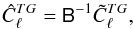 (25)where
 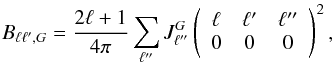 (26)with
  the cross-angular power spectrum of the T and G masks.
The estimator in Eq. (25) is nearly optimal because has to be understood as the mean value over an ensemble average of skies. When more than a single CAPS is considered, for instance, when one is interested in the cross-correlation of the Planck CMB map with more than one LSS tracer map, the CAPS estimator can be seen as a single vector with Nℓmax components, with N being the number of surveys.
It can be shown that the element Cℓℓ′,ij of the covariance matrix of the CAPS estimator in Eq. (25) (for the case of a masked sky and for N surveys) is given by 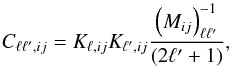 (27)where
 ![\begin{equation} K_{\ell, i j} = \left[ C_{\ell}^{{TG}_i}C_{\ell}^{{TG}_j} + C _{\ell}^{T}\left(C_{\ell}^{{G}_i {G}_j} + N_{\ell}^{{G}_i {G}_j}\delta_{ij} \right) \right]^{1/2}\!,\label{eq:cov_caps2} \end{equation}](/articles/aa/full_html/2014/11/aa21526-13/aa21526-13-eq237.png) (28)and
(28)and  is the (ℓ,ℓ′) element of the inverse matrix of M for surveys i and j fixed, such as
 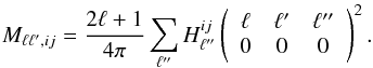 (29)Here
  is the angular cross-power spectrum of the two joint masks, that is, the masks resulting from the multiplication of the T with Gi and Gj, respectively. The quantities
  are expected or fiducial spectra,
  is the Poissonian noise of the y survey (deconvolved by any beam or pixel filter), and δij is the Kronecker delta. In Eq. (28), the instrumental noise associated with the CMB data has been ignored, since the Planck sensitivity is such that the noise contribution on the scales of interest is negligible. When more than one survey has poor sky coverage, then the complexity of the correlations is not well reflected by the previous expression. Therefore, we computed Cℓℓ′,ij from coherent CMB and LSS Monte Carlo simulations. For each simulation, we generated four independent, Gaussian, and white realizations (at Nnside = 64), which were afterwards properly correlated using the expected auto- and cross-correlations of the signals. Corresponding Poissonian shot-noise realizations were added to each survey map. The resulting four maps were masked with the corresponding masks (i.e., one for the CMB and one for mask for each survey).
The computation of the CAPS in Eq. (25) is extremely fast (especially for the resolutions used in the study of the ISW). However, as stated above, it is only a nearly optimal estimator of the underlying CAPS. Moreover, its departure from optimality is largest at the smallest multipoles (largest scales), where the ISW signal is more important.
The QML angular power spectrum
The QML method for the power spectrum estimation of temperature CMB anisotropies was introduced by Tegmark (1997) and later extended to polarization by Tegmark & de Oliveira-Costa (2001). For an application to temperature and polarization to WMAP data see Gruppuso et al. (2009) and Paci et al. (2013). The same method was employed to measure the cross-correlation between the CMB and LSS in Padmanabhan et al. (2005), Ho et al. (2008), and Schiavon et al. (2012). The QML method is usually stated to be optimal, since it provides unbiased estimates and the smallest error bars allowed by the Fisher-Cramér-Rao inequality. As a drawback from the computational point of view, the QML is a very expensive approach. We denote the QML estimator of the CAPS between the CMB map T and an LSS tracer G (at multipole ℓ) by  (i.e.,
  for this cross-correlation estimator).
A detailed description of the algebra of the QML is given in Schiavon et al. (2012). We briefly recall here the basics of the CAPS estimator, which is given by ![\begin{equation} \label{eq:qmlcaps} \hat{Q}_\ell^{{TG}} = \sum_{\ell' X'} (F^{-1})^{{{TG}} ~ X'}_{\ell\ell'} \left[ \vec{x}^{T} \tens{E}_{\ell'}^{X'} \vec{x} -{\rm Tr}(\tens{N}\tens{E}_{\ell'}^{X'}) \right], \end{equation}](/articles/aa/full_html/2014/11/aa21526-13/aa21526-13-eq252.png) (30)where X represents any of the following spectra: X = {T,TG,G}. The vector x has 2Npix elements (with Npix being the total number of pixels allowed by the joint CMB and LSS mask): the first set of Npix corresponds to the CMB map, and the second one accounts for the LSS map. The
(30)where X represents any of the following spectra: X = {T,TG,G}. The vector x has 2Npix elements (with Npix being the total number of pixels allowed by the joint CMB and LSS mask): the first set of Npix corresponds to the CMB map, and the second one accounts for the LSS map. The  is the Fisher matrix defined as
 ![\begin{equation} \label{eq:fisher} F_{\ell\ell'}^{{TG}~ X'}=\frac{1}{2}{\rm Tr} \left[\tens{C}^{-1}\frac{\partial {\tens{C}}}{\partial C_\ell^{{TG}}}\tens{C}^{-1}\frac{\partial \tens{C}}{\partial C_{\ell'}^{X'}}\right], \end{equation}](/articles/aa/full_html/2014/11/aa21526-13/aa21526-13-eq259.png) (31)and the E matrix is given by
(31)and the E matrix is given by 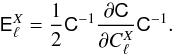 (32)The object
  is the global covariance matrix, including the signal S and noise N contributions, with
  being the fiducial theoretical angular power spectrum. The uncertainties in the QML estimates are given by the inverse of the Fisher matrix, which includes the correlation among different multipoles. The error associated with the shot noise of the galaxy surveys is modelled in the galaxy submatrix of N.
The results presented here are based on  , while
  is used as a cross-check, applied to a lower-resolution version of the maps of Nside = 32. In addition, the maximum multipole considered in this case is ℓmax = 2Nside, which has been already verified as a conservative limit for the QML.
4.1.2. Cross-correlation function
The cross-correlation function (CCF) is a suitable tool for studying the ISW effect via cross-correlation of the CMB fluctuations and tracers of the LSS, and it has been one of the most extensively used in this context (e.g., Boughn & Crittenden 2002; Giannantonio et al. 2008; Xia et al. 2009). On the one hand, the signal only appears at very large scales and, therefore, it is sufficient to work at resolutions at which the low performance of the CCF (in terms of computational time) is not a serious handicap. On the other hand, neither the CMB nor the LSS data are available with full sky coverage and, in some cases, the geometry of the masks is very complicated: the CCF adapts perfectly to the effects of partial sky coverage, since it is defined in real space. As a drawback, the Poissonian noise of the galaxy tracer appears at the smallest angular scales, where the signal-to-noise ratio of the ISW effect is higher for this estimator. Therefore, a proper characterization of the shot-noise is especially important for the CCF to obtain a good estimation of the uncertainties.
We denote the CCF between the CMB map T and an LSS tracer G (at an angular distance of θ) as CTG(θ) (i.e.,  for this cross-correlation statistic). The CCF estimator is defined as
 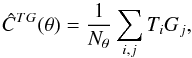 (33)where the sum runs over all pixels with a given angular separation. For each angular bin centred around θ, Nθ is the number of pixel pairs separated by an angle within the bin. Only the pixels allowed by the joint CMB and LSS mask are considered. The angular bins used here are θ1 ∈ [0,1]°; θ2 ∈ (1,3]°; θ3 ∈ (3,5]°; ...; and θ61 ∈ (119,121]°. The choice of binning does not affect the results significantly.
The covariance of the CCF estimator can be easily derived from the one already computed for the CAPS in Eq. (27). It is sufficient to know that the CCF can be expressed in terms of the CAPS as 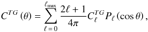 (34)where Pℓ(cosθ) are the Legendre polynomials. Hence, it is straightforward to prove that the covariance between the θ and θ′ components of the CCF for the surveys i and j, respectively, is given by
 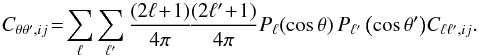 (35)
(35)
4.1.3. Wavelet covariance
Wavelets provide an interesting alternative to more traditional tools (e.g., CCF or CAPS) for studying the CMB-LSS correlation. They exploit the fact that the ISW signal is mostly concentrated at scales of a few degrees (e.g., Afshordi 2004). Wavelets are ideal kernels to enhance features with a characteristic size, since the wavelet analysis at an appropriate scale R amplifies those features over the background. Therefore, wavelets could provide most of the signal-to-noise ratio of the ISW effect by just analysing a narrow range of scales. They were first proposed for the ISW detection by Vielva et al. (2006), where the SMHW (Martínez-González et al. 2002) was proposed as the filtering kernel. The basic idea of this approach is to estimate the covariance of the SMHW coefficients (SMHWcov) as a function of the wavelet scale (see e.g., Vielva et al. 2006, for details). Other wavelet kernels can be considered, such as needlets (Pietrobon et al. 2006a), directional wavelets (McEwen et al. 2007), or steerable wavelets (McEwen et al. 2008).
We denote the SMHWcov between the CMB map T and a LSS tracer G (at a wavelet scale R) as  , i.e.,
  for this cross-correlation statistic). The SMHWcov estimator is defined as
  (36)where
  and
and  are the SMHW coefficients for the CMB and the LSS at scale R, respectively (note that wavelet coefficients are forced to have zero mean on the observed sky). The scales considered in our study are R = { 60, 90, 120, 150, 200, 250, 300, 350, 400, 500, 600 } in arcminutes.
As for the CCF, the covariance of the SMHWcov estimator can be easily derived from the one already computed for the CAPS in Eq. (27). It is sufficient to know that the SMHWcov can be expressed in terms of the CAPS as  (37)where
  is the SMHW window function at the scale R. Hence, it is straightforward to prove that the covariance between the R and R′ components of the SMWHcov for surveys i and j, respectively, is given by
  (38)
(38)
4.2. Cross-correlation tests
For any of the cross-correlation estimators described above, we performed two different statistical tests. First, if the observed cross-correlation is given by  , a simple χ2 can be proposed to estimate the amplitude A, such that
  is the closest solution to :
 ![\begin{equation} \chi^2\left(A\right) = \left[\hat{\xi}_a^{xy} - A\xi_a^{xy} \right]^{T} \tens{C}_{\xi^{xy}}^{-1} \left[\hat{\xi}_a^{xy} - A\xi_a^{xy}\right]\!, \label{eq:xcorr_fit} \end{equation}](/articles/aa/full_html/2014/11/aa21526-13/aa21526-13-eq297.png) (39)where Cξxy is the covariance matrix (of dimension amax × amax) of the expected cross-correlation , that is,
(39)where Cξxy is the covariance matrix (of dimension amax × amax) of the expected cross-correlation , that is,  . It is straightforward to show that the best-fit amplitude A and its dispersion are given by
![\begin{eqnarray} \label{eq:fit} &&A=\left[\hat{\xi}_a^{xy}\right]^t \tens{C}_{\xi^{xy}}^{-1} \xi_a^{xy} \left[\left[\xi_a^{xy}\right]^t \tens{C}_{\xi^{xy}}^{-1} \xi_a^{xy} \right]^{-1}\!, \\ &&\sigma_A=\left[\left[\xi_a^{xy}\right]^t \tens{C}_{\xi^{xy}}^{-1} \xi_a^{xy} \right]^{-1/2} \nonumber\!. \end{eqnarray}](/articles/aa/full_html/2014/11/aa21526-13/aa21526-13-eq301.png)
An analogy with Eq. (39) can be defined for the null hypothesis case: ![\begin{equation} {\chi^2}_{\mathrm{null}} = \left[\hat{\xi}_a^{xy}\right]^{T} \tens{D}_{\xi^{xy}}^{-1} \hat{\xi}_a^{xy}, \label{eq:xcorr_null} \end{equation}](/articles/aa/full_html/2014/11/aa21526-13/aa21526-13-eq302.png) (41)where Dξxy is the covariance of the cross-correlation of the two signals, in the absence of an intrinsic dependence, that is, when
(41)where Dξxy is the covariance of the cross-correlation of the two signals, in the absence of an intrinsic dependence, that is, when  . The ISW signal is very weak and, therefore it is a good approximation to assume that Dξxy ≈ Cξxy.
For Gaussian statistics, χ2null already provides the direct probability of the observed cross-correlation under the null hypothesis. However, several problems (sky coverage, systematics, foregrounds residuals, etc.) forced us to use alternative approaches to estimate the probability. One of the most common options is to perform the cross-correlation of survey signal y with realistic simulations of the CMB, x, and compute a joint statistics (e.g., χ2null) for each simulation. The probabiltiy value associated with the data is then the fraction of simulations with a value of χ2null equal to or higher than the one obtained for the data. Both Cξxy and Dξxy can be derived either analytically or numerically (via simulations).
The latter approach is computationally expensive, but in some cases could provide a more accurate defence against certain systematics, in particular, the incomplete sky coverage. There are several options to perform this type of simulations. The standard approach is the one mentioned above, that is, cross-correlation of the LSS map with CMB simulations. This is a very reliable approach, since it is usually hard to reproduce the systematics present in the LSS tracers, but incomplete because the LSS is fixed, resulting in a lack of randomness. An alternative method is to use a jack-knife test, which unfortunately tends to underestimate the errors. Finally, one can produce simulations of both the CMB and the LSS, assuming perfect knowledge of the properties of both signals, in particular of the LSS field (which, as mentioned above, is almost never the case). Comprehensive discussions of these approaches are given in Cabré et al. (2007) and Giannantonio et al. (2008).
4.3. Results
Expected significance A/σA of the CMB-LSS cross-correlation.
In this section we present the results obtained from the cross-correlation of the galaxy catalogues described in Sect. 2.2 (NVSS, SDSS-CMASS/LOWZand SDSS-MphG) with the four Planck CMB maps presented in Sect. 2.1.1 (C-R, NILC, SEVEM, and SMICA). All these maps were analysed at a HEALPix resolution of Nside = 64. The cross-correlation estimators described in the previous section were applied to all cases. This comprehensive analysis will help to achieve a reliable estimate of the ISW.
As already mentioned, the covariance among all the components of the estimators were obtained from coherent Gaussian simulations of the CMB and the three galaxy catalogues. Since we only considered large-scale effects (above about 1°), the same set of CMB simulations are equally valid for the four CMB maps, since they are nearly identical on such scales (see Planck Collaboration XII 2014, for details). We used 70 000 coherent Monte Carlo simulation sets (as described in Sect. 4.1.1) to compute the correlations; this is enough to characterize the covariance.
The expected signal-to-noise ratio for the ISW effect detection is summarized in Table 4. Values for all the cross-correlation estimators are given. We considered a survey-by-survey detection as well as the joint analysis of all the surveys. A signal-to-noise ratio of about 3σ is expected for the joint analysis, which is dominated by the NVSS cross-correlation. This is expected, since, firstly, NVSS covers a much larger portion of the sky compared to other surveys, and secondly, it extends over a redshift interval ideal for the detection of the ISW signal (e.g. Afshordi 2004).
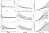 |
Fig. 5 Observed and expected cross-correlation signal versus multipole ℓ for several surveys and different cross-correlation estimators. Columns from left to right correspond to CAPS, CCF, and SMHWcov. Rows from top to bottom represent NVSS, SDSS-CMASS/LOWZ, and SDSS-MphG. In each panel we show the expected cross-correlation (black line) and the ±1σ region (grey area). |
The differences among estimators are not significant, indicating that none of them is clearly better than the others. To explore this agreement further, we analysed an extra set of 1000 CMB and LSS clustered simulations and compared, simulation by simulation, the ISW amplitude estimation derived for each cross-correlation estimator ( ,
,  and
and  ). In Table 5 we summarize the comparison. We only report values for the joint fit to the ISW amplitude for the three surveys. Similar results are found survey by survey. For each pair of estimators, we provide the mean difference among the amplitude estimations (ΔA), the dispersion of these differences (sA), the ratio (η) of this dispersion to the expected sensitivity (i.e., the inverse of the signal-to-noise ratio numbers given in the last column of Table 4), and the correlation coefficient (ρ). It is clear that the agreement between estimators is very high and that differences are, on average, lower than half the statistical uncertainty imposed by the sampling variance.
For each pair of estimators, we give the mean difference among the amplitude estimate (ΔA), the dispersion of these differences (sA), the ratio (η) of this dispersion to the expected sensitivity (i.e., the inverse of the signal-to-noise ratio numbers given in the last column of Table 4), and the correlation coefficient (ρ).
We fitted the observed cross-correlations to the expected ISW signal (, , and , see Fig. 5), following Eq. (40), that is, allowing for a free amplitude of the expected signal. Results are summarized in Table 6. Note that the plots only show partial information on the total detection level of the ISW signal, specifically those from the diagonal of the covariance matrix Cξxy. The level of correlation among the components (i.e., the multipoles, angles or scales) varies considerably for the different estimators, and, therefore the whole picture is only obtained when the full covariance is considered, as in Eq. (40).
Overall, the ISW detection is at about the 3σ level and, as expected, it is clearly dominated by the NVSS signal. There are only small differences among estimators and CMB maps (as expected from the above discussion), indicating that this is a reliable result. Note that all the estimated amplitudes are compatible with unity within the error bars (especially for NVSS and SDSS-CMASS/LOWZ). This is an additional validation of how CMB and LSS are modelled. Values of A that deviate significantly from unity would indicate some tension between the observed cross-correlation and the model (in particular on the LSS modelling, which is more complex). The CAPS-QML, applied to the SEVEM and NVSS (i.e., the survey with the highest signal-to-noise ratio), yields a value of A = 0.73 ± 0.33, which is compatible with the CAPS when applied to the same Nside = 32 and ℓmax = 2Nside resolution (A = 0.84 ± 0.34). Preliminary tests indicated that running the CAPS-QML at Nside = 64 resolution may increase the sensitivity for detecting the ISW effect with NVSS by ≈20%.
Amplitudes A, errors σA, and significance levels A/σA of the CMB-LSS cross-correlation (survey-by-survey and all together) generated by the ISW effect for all component separation algorithms for the different estimators.
Our results indicate a somewhat lower signal-to-noise ratio than in some previous analyses of WMAP data, where several (and in some case quite similar) surveys were also considered. For instance, Ho et al. (2008) and Giannantonio et al. (2012) found 3.7σ and 4.4σ detections, respectively. Compatibility with the former is below 1σ, while there is more tension (about 1.5σ) with the latter. A fraction of about 0.3σ of these differences might be explained in terms of the comological parameters adopted to defined the theoretical expectations. In particular, the lower values of H0 and ΩΛ found by Planck (Planck Collaboration XVI 2014) with respect to WMAP (e.g., Larson et al. 2011) imply a lower sensitivity for the ISW by ≈10%. The rest of the differences come either from the LSS side or from the error characterization, which depends on the presence of a correlated signal between CMB and LSS simulations (see for instance Cabré et al. 2007, for a discussion). Survey modelling is another important aspect: in addition to systematic errors associated with the galaxy identification and redshift estimation procedures, there are complicated aspects, such as the bias characterization. As was mentioned already, a strong point of our results is the excellent compatibility between the ISW amplitude estimates with respect to the expected value. While our estimation deviates by about 0.5σ from the expected value, the Giannantonio et al. (2012) result exceeds it by about 1σ and Ho et al. (2008) is higher by 2σ.
Nevertheless, the value of the ISW effect that we measured by means of NVSS (which is probably the best current catalogue for studying the ISW effect because of its large sky coverage, redshift range, and density of galaxies) is significant and agrees with previously published results using WMAP.
We also studied the ISW signal from the point of view of its compatibility with the null hypothesis. We considered in this analysis only the NVSS catalogue, since it provides the highest detection of the ISW effect and therefore is the best-suited of the existing surveys to challenge the null hypothesis. Probability values are summarized in Table 7. As mentioned in Sect. 4.2, there is no unique way of computing the null hypothesis. Our approach follows Eq. (41), where Dξxy was computed out of 90 000 CMB simulations that were cross-correlated with the LSS data. This matrix was used to compute  from the data. This value was then compared with its distribution for the null hypothesis, obtained from 1000 realistic CMB simulations (FFP-6) uncorrelated with NVSS, which were processed in the same way as the Planck data set. CAPS provides the lowest probability value, but the null hypothesis is rejected at about 10% only; this result is expected since the ISW effect is weak.
The fact that the CAPS statistic provides tighter limits than the CCF and SMHWcov could have been anticipated. In our implementation, the CAPS explores the maximum angular range allowed for a given map, while the CCF and the SMHWcov approaches are only evaluated at certain angles/scales. This limitation is not a problem in the analysis devoted to estimating the ISW amplitude, since these angles/scales are suitable for detecting the ISW. However, to discard the null hypothesis, the larger the number of “distances”, the better.
The previous approach is a frequentist one. However, there is an alternative way of addressing the null hypothesis compatibility in the framework of a hypotheses test. In particular, we can study the ratio of Bayesian evidence for both scenarios, comparing the alternative (there is ISW signal) and the null (there is no correlation between the CMB and the LSS) hypotheses. To compute the Bayesian evidence we just need the likelihoods and the priors associated with each hypothesis, which are already available. The likelihood for the alternative hypothesis is obtained from Eq. (39), peaked at the best-fit value for the ISW amplitude, and its prior can be described as a Gaussian probability peaked at A = 1 and with a dispersion given by σA in Eq. (40). Conversely, the likelihood for the null hypothesis is the function given by Eq. (41), and its prior would be like the one for the alternative hypothesis, but peaked at A ≡ 0 (notice that this is justified, since, as explained in the previous section, Dξxy ≈ Cξxy). Following this approach, we obtain a Bayesian evidence ratio of about 30, which provides strong support for the assumption that there is an ISW signal.
Probability values of the CMB-LSS cross-correlation for the NVSS survey under the null hypothesis for the four component separation methods and for the different estimators.
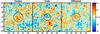 |
Fig. 6 Stacked regions of Planck maps corresponding to the locations of the superstructures identified by GR08. From left to right we show the images resulting from stacking of the 50 superclusters, the 50 supervoids, and the difference of the two. The black circles superimposed indicate the angular radius at which the signal-to-noise ratio is highest. See Fig. 7 for the corresponding temperature and photometry profiles, as well as their statistical significance. |
5. Stacking of large-scale structures
An alternative approach for measuring the ISW effect in Planck maps is to search for an ISW signal directly at the positions of positive and/or negative peaks in the potential. Since the expected (and observed) signal is very weak, a stacking technique needs to be applied for individual structures. Using the WMAP data, it has been shown that CMB maps show hot spots and cold spots in the direction of superclusters and supervoids, respectively (Granett et al. 2008a,b, GR08 hereafter), which appear to be barely consistent with the predictions of standard ΛCDM (see also Hernández-Monteagudo & Smith 2013). These structures, which are not yet virialized, are evolving while the CMB photons travel across them and this should contribute to the ISW effect. We applied here the same approach to the different Planck maps, using the catalogues of superstructures introduced in Sect. 2.2.4, and we tested the reliability of our findings. We first discuss our method and the results obtained using the catalogue provided by GR08 and then present the results obtained with the other catalogues.
5.1. Method
Our analysis was performed on the SMICA CMB map, although we verified that the results are compatible for the other three Planck maps. We also used the cleaned frequency maps from SEVEM (see Sect. 2.1.1) for some of the tests. We first removed the monopole and dipole of the maps (outside the U73 mask) and then applied a compact source mask based on the Planck Legacy Point Source Catalogue (Planck Collaboration XII 2014) to remove the contamination from individual point sources.
For the purpose of comparison with the results of GR08, we smoothed the CMB maps with a common Gaussian kernel of 30′ FWHM. We then projected them onto patches around each position in the supervoid and supercluster catalogue. The GR08 structures have a relatively small size on the sky (a few degrees), but the other two catalogues considered here contain many larger and closer voids, covering larger angular sizes. Therefore we worked with 30deg × 30deg CMB patches and chose the pixel size to be 6′, so that all voids considered are fully enclosed. We then co-added (stacked) the maps, taking into account the mask used. On the stacked images, we calculated both the radial temperature profile and the aperture photometry to characterize the signal around density structures. The temperature profile was obtained by computing the mean of the pixels in rings of fixed width and increasing angular radius; in practice, it was calculated for 150 radii between 0deg and 15deg, with a width of  . The photometry profile was obtained by applying a compensated filter that subtracts the average temperature of a ring from the average temperature within the disk, whose radius θ is the inner radius ring, and where the outer radius was chosen to be
  , so that the disc and ring have the same area. This is expected to enhance fluctuations of typical angular size θ against fluctuations at smaller or larger scales. Aperture photometry results were also provided for at 150 angles, this time between 0deg and 15/
 . In addition to the monopole and dipole, we also removed from the CMB maps the contribution of large-scale angular modes, namely ℓ = 2 − 10. These modes correspond to angular scales much larger than those of the structures under investigation, and for our purposes their only effect is to introduce gradients in the stacked images; the high-pass filter essentially stops from gradients entering the stacked map (which is equivalent to removing gradients at the end). The contribution of the large-scale angular modes has no impact on the aperture photometry profiles and only introduces an offset in the temperature profiles (Ilić et al. 2013).
To estimate the significance of the resulting photometry and temperature profiles, we followed a Monte Carlo approach based on stacked CMB images chosen at random positions. In detail, we computed the photometry and the temperature profiles for 16 000 sets of 50 CMB patches randomly distributed over the SDSS area. We then compared the profiles obtained from the stacking at the location of the GR08 superstructures to these random profiles to compute their signal-to-noise ratio.
5.2. Results
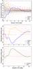 |
Fig. 7 Temperature (top) and photometry (middle and bottom) profiles of the stacked CMB patches at the location of the 50 supervoids and 50 superclusters of GR08. The lower panel shows the combined photometry profile (i.e., the average cluster profile minus the average void profile). The significance is represented by 1, 2, 3, and 4σ level curves (dashed and dotted lines represent positive and negative error bars, respectively). These curves represent the dispersion of the 16 000 stacks of 50 CMB patches chosen at random positions (for illustration, we represent in grey 300 of the random profiles in the top panel). |
We show in Fig. 6 the stacked images of the 50 supervoids and 50 superclusters of GR08 in the Planck map. The corresponding temperature and photometry profiles along with their significance levels are shown in Fig. 7. First, although the signatures are fairly weak, the sign of the effect certainly seems to be correct. Using the same catalogue and the Planck CMB map, we found a reasonable agreement with GR08. The highest photometric decrement −10.8 μK (essentially identical with the −11.3 μK found by GR08) induced by supervoids is obtained for a preferred scale of about  (4deg in GR08) and a signal-to-noise ratio of 3.3 (3.7σ in GR08), as shown in Fig. 7. Superclusters produce a photometric increment of about 8.5 μK (slightly above the 7 μK in GR08), with a significance of 3.0σ (compared with 2.6σ in GR08) at a slightly larger angle of
  . Finally, the stack of the combined sample (clusters minus voids) gives a temperature deviation of 8.7 μK with a signal strength of 4.0σ at
  , which is consistent with the values reported in GR08. The values of statistical significance for our aperture photometry results are closely related to those for the temperature profiles. Indeed, as shown in the top panel of Fig. 7, the temperature profile for the void stack shows a deficit of about 2σ at small angular radii and an excess of about 2σ extending to large radii. Since the aperture photometry is essentially an integral of the temperature profile with a compensated filter, it picks up enhanced significance because of the shape of the temperature profile.
As noted previously by several authors (e.g., Hernández-Monteagudo & Smith 2013), the amplitude and shape of the photometric profile found for voids and clusters disagrees (around 2σ) with the values expected from pure ISW within ΛCDM. However, it is not straightforward to associate this entire signal with a pure ISW effect. As seen in the Fig. 6, many small-scale structures – both cold and hot – are present around the region delineated by the angular radius at which the signal-to-noise ratio of the aperture photometry is highest. This small-scale structure contributes to the amplitude of the photometric decrement, but at a few tens of μK, which is incompatible with the ΛCDM predictions for the ISW effect. These are rather simply background CMB fluctuations, and linger because of the small number (50) of patches that were used to produce the stack.
It is intriguing that the angular sizes of the catalogued superstructures are smaller than the angular sizes suggested by the photometry profiles. This result was more apparent when we repeated the stacking analysis after rescaling each CMB patch by the effective radius of the structure it contains. Since the voids and super clusters identified by GR08 are approximately the same size, the photometric results are similar after rescaling (−10 μK for voids and 7.9 μK for superclusters). However, the deviations have significance levels of 3.3σ and 2.7σ for supervoids and superclusters, respectively, at angular sizes of 0.9 (voids) and 2.6 (clusters) times the effective radius of the structures. This mismatch, especially for clusters, could be a result of underestimation of the structure extent of the ZOBOV and VOBOZ algorithms (as previously suggested by GR08) or because larger potential hills and valleys underlie the detected superstructures. Since structure in the potential is related to the density field through the Poisson equation, gravitational potential features are expected to cover larger scales than structures in the density field. Nevertheless, the factor of 2.6 for the case of superclusters seems high. It is also true that the GR08 superstructures were identified in the LRG subsample of the SDSS, and LRGs are known to be biased tracers of the matter density field (e.g., Tegmark et al. 2006). This bias might help to explain why structures are larger than the scales identified by the VOBOZ algorithm, although the argument would go in the opposite sense for the voids. Another way of stating this is (Hunt & Sarkar 2010) that the relatively strong effect decrement found for the GR08 voids can only be attributed to the ISW effect if the underdensities have been significantly underestimated or if the LRGs are under-biased.
It is therefore difficult to be confident that the signal is caused entirely by the ISW effect. We know, however, that the ISW signal generated by superstructures is expected to be achromatic, since it generates a fractional perturbation of the CMB temperature. To determine if the signal we measure is indeed independent of frequency, we applied the same technique to Planck individual SEVEM cleaned frequency maps from 44 to 353 GHz. Lower (higher) frequency maps may be contaminated by radio (IR) signals coming from our Galaxy and may thus introduce a bias in the measurement. Figure 8 shows the photometry profiles of supercluster- and supervoid-stacked maps at 44, 70, 100, 143, 217, and 353 GHz. The flux measured appears to be quite constant, which supports the idea that the signal is generated by the ISW effect induced by structures. In the remainder of this section, we therefore apply our analysis only to the SMICA CMB map.
5.3. Discussion and alternative catalogues
We that although the GR08 structures are considered to be good tracers of the cosmic matter distribution on scales larger than 10 h-1 Mpc, they are also known for their sparsity at these redshifts (z ≈ 0.4–0.7). This sparsity could lead to biased estimates of the properties of the reconstructed voids, their sizes and depths in particular could be biased. Moreover, some of the structures overlap on the sky, which could lead to systematic effects in the stacking analysis.
We therefore turned to other samples, for example, to the catalogue of Pan et al. (2012) introduced in Sect. 2.2.4. The 1054 statistically significant voids it contains are larger than 10 h-1 Mpc in radius and, with redshifts lower than 0.1, they are much closer to us than the structures of GR08. Direct stacking gives only a weak signal at about the 1σ level, which is difficult to reconcile with the previous results. This may be due to the inclusion of a large number of small voids that may dilute the signal. Moreover, unlike the voids of GR08, the voids of Pan et al. (2012) have a large scatter in angular sizes on the sky, from about 2deg to 20deg (e.g., Ilić et al. 2013). To try to enhance the signal, we repeated the stacking after rescaling the voids to their effective sizes. We also subdivided the catalogue into subsamples based on redshift, radius, and/or angular size. However, none of these attempts yielded any statistically significant result, in agreement with Ilić et al. (2013).
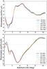 |
Fig. 8 Coherence of the signal across the SEVEM frequency channels. The aperture photometry profiles measured in the stacked patches centred on superclusters (top) and supervoids (bottom) are virtually identical for all frequencies, as it is expected for the ISW signal. |
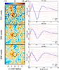 |
Fig. 9 Stacked images (left) and photometry profiles (right) obtained for the voids of Sutter et al. (2012) after rescaling. From top to bottom, we show results obtained from stacking the largest 231, 589, and 936 voids. The black superimposed circles indicate the angular radius in terms of the effective radius after rescaling, at which the signal is highest. The statistical dispersion is reduced when more voids are stacked. However, the amplitude of the cold spot at about 0.5 times the effective void radius is mostly due to the surrounding hot shell, which is easiest to see in the bottom panel. This is also demonstrated by the 3σ signal detected using aperture photometry, seen at radii above 1.2 times the effective radius (for the case with 936 void). Dashed and dotted lines in the right-hand panels represent positive and negative error bars, respectively, from 1 to 4σ. |
Finally, we applied our procedure to the catalogue of voids published by Sutter et al. (2012). These cover a rather extended range of angular scales (about 2–10deg), and accordingly we rescaled all the CMB patches by the effective radius of each void. Stacking subsample by subsample (dim1, dim2, bright1, bright2, lrgdim, lrgbright) did not yield any significant signal. Similarly, when stacked together, the entire catalogue does not yield an ISW detection. However, since the ISW signal is expected to be stronger for the largest and closest voids (e.g., Flender et al. 2013) we tried starting from the largest void and adding them one by one, looking for the optimal number of voids, that is, that for which the signal-to-noise ratio is highest (see Fig. 10). We found that stacking 231, 589, or 936 voids gives about the same signal-to-noise ratio (2.5σ, 2.0σ and 2.2σ, respectively). However, the more voids we stacked, the smaller was the amplitude of the photometry signal (see Fig. 9, this was about −2.0 μK for 936 voids, −2.1 μK for 589 voids and −4.1 μK for 231 voids, at an angular size of about 0.5 times the common rescaled radius. These amplitudes are lower than those found with the 50 GR08 voids, but higher than expected from numerical simulations (see e.g., Hernández-Monteagudo & Smith 2013, for higher redshift and larger voids), but see also Cai et al. (2013).
The apparent angular size detected (about 0.5 times the effective void radius) in the photometry profile is smaller than that for the GR08 voids, but agrees with expectations from simulations (Cai et al. 2013) and is consistent with the sizes detected using WMAP data (Ilić et al. 2013).
The profiles in Fig. 9 show intriguing hints (significance about 2σ) of a positive excess below about 0.2 times the effective void radius. This is somewhat surprising, since the centre of each void of the Sutter et al. (2012) catalogue has been defined as the volume-weighted barycentre of all the galaxies contained in the void volume. This definition in principle removes most of the bias that may arise in other methods, such as choosing the most underdense galaxy position, which would lead to a slight overdensity at the centre. Figure 9 also shows positive excess for larger apertures, partly caused by the large hot ring surrounding the cold feature in the stacked images, which raises the mean temperature of the stacked image for discs of radii of about 0.8−1.2 times the void radius.
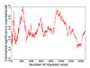 |
Fig. 10 Estimate of the optimal number of patches/voids to stack using the catalogue of Sutter et al. (2012). Starting from the largest void and adding one CMB patch at a time to the stack, we find at each step N the minimum of the aperture photometry profile and multiply this value by |

6. ISW map recovery
In recent years, some effort has been invested not only to obtain the statistical cross-correlation signal between the CMB and LSS data, but also to recover a map of the ISW signal itself (Barreiro et al. 2008, 2013; Francis & Peacock 2010a; Dupé et al. 2011). In particular, assuming the existence of a correlation between the CMB and the gravitational potential, it is possible to recover a map of the ISW fluctuations using a filtering method when one has a tracer of the gravitational potential (e.g., the galaxy catalogues described in Sect. 2.2) and the CMB fluctuations. Given the weakness of the signal, the main objective of this section is to provide a qualitative image of the ISW fluctuations for visual inspection, and an additional consistency test of the validity of the assumed fiducial model, by comparing the statistical properties of the recovered and expected signals. In addition, this secondary anisotropy map can also be used to study the large-scale properties of the CMB and its possible relation to some possible large-angle anomalies found in the Planck data (Planck Collaboration XXIII 2014).
6.1. Method
We followed the methodology of Barreiro et al. (2008), which applies a linear filter to the CMB and to a gravitational potential tracer map to reconstruct an ISW map, assuming that the cross- and auto-spectra of the signals are known. This technique has recently been applied to reconstruct the ISW map from the WMAP data and NVSS galaxy map (Barreiro et al. 2013). The filter was implemented in harmonic space and the estimated ISW map ŝℓm at each harmonic mode is given by (see Barreiro et al. 2008 for details) 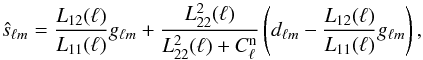 (42)where L(ℓ) corresponds to the Cholesky decomposition of the covariance matrix between the considered tracer of the potential and the ISW signal at each multipole, which satisfies C(ℓ) = L(ℓ)LT(ℓ). Here dℓm and gℓm are the CMB data and the gravitational potential tracer map, respectively, and
  is the power spectrum of the CMB signal excluding the ISW effect. If full-sky coverage is not available, the covariance matrix is obtained from the corresponding pseudo-spectra. It can be shown that the expected value of the power spectrum for the reconstructed signal is given by
 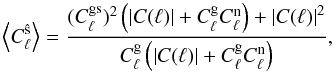 (43)where | C(ℓ) | is the determinant of the tracer-ISW covariance matrix at each multipole, and
  and
and  are the assumed cross-spectrum and gravitational potential tracer spectra, respectively. Note that the recovered ISW power spectrum will not contain the full ISW signal, since it can only account for the part of the ISW signal probed by the tracer considered. It is also worth noting that in detail the expected cross-correlation depends on the assumed model. However, in practice, given the weakness of the signal, it would be difficult to distinguish between two mild variants of the standard ΛCDM model. Nevertheless, this approach still provides a useful consistency check.
6.2. Results
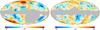 |
Fig. 11 Reconstructed ISW map from the Planck CMB and NVSS data (left) and from the Planck CMB and lensing potential maps (right). Note that the maps are not expected to look exactly the same, since each of them provides a partial reconstruction of the noisy ISW signal (see Sect. 6.2 for details). |
We applied the filter described above to two different cases: combining information from the CMB and the NVSS galaxy catalogue, and applying the filter to the CMB and the recovered lensing potential map described in 2.1.2. Results were obtained for the four Planck maps, C-R, NILC, SEVEM, and SMICA. For simplicity, we show the reconstructions only for the SEVEM CMB map, since the four methods give very similar results. The resolution considered for both analyses is Nside = 64.
For the first case, we used the Planck fiducial model for the CMB and cross-power spectrum, while for the NVSS map we assumed the model described in Sect. 2.2.1. We also took into account the presence of Poissonian noise. We excluded the area obtained from combining the CMB mask at Nside = 64 (described in Sect. 2.1.1) and the area that has not been observed by NVSS. The final mask represents about 62% of the sky. Since the filter is constructed in harmonic space, we used an apodized version of the mask to reduce the mask-induced correlations. In any case, the degradation introduced by a mask is small (Barreiro et al. 2008).
For the second case, the lensing map involved applying a high-pass filter, which removed all multipoles with ℓ < 10. This filtering was made in harmonic space with a mask. To take this effect into account we used a direct estimate of the pseudo-power spectrum of these data for the power spectrum of the lensing map after applying the corresponding apodized mask. We used the Planck fiducial model for the other power spectra involved, but set the cross-power for ℓ < 10 to zero. A mask wasconstructed by combining the CMB mask plus that provided for the lensing potential map (described in Planck Collaboration XVII 2014), which represents about 67% of the sky. The corresponding apodized version of this mask was applied before reconstructing the ISW map. Note that the map given in Fig. 1 (right panel) corresponds, to a good approximation, to the first term of the right-hand side of Eq. (42).
Figure 11 shows the reconstructed ISW map using the Planck CMB map and NVSS (left panel) and that obtained combining the CMB with the lensing potential map (right panel). There are similar structures present in both maps, but they are not expected to look exactly the same, since each of them provides only a partial reconstruction of the ISW signal. This is because that the reconstruction accounts for the part of the ISW effect probed by the considered tracer, which is different (although correlated) for each case. Moreover, because of the high-pass filter applied to the lensing potential map, the power at ℓ < 10 for this case corresponds to the Wiener-filtered map of the CMB (to which the filter given by Eq. (42) defaults, if the cross-correlation is set to zero, as in this case), without additional information from the considered tracer.
For both cases, we tested that the power spectrum of the recovered ISW signal, as well as that of the cross-power between the reconstructed ISW and the considered gravitational potential tracer, are consistent with the corresponding expected values. This indicates the compatibility between the assumed fiducial model and the underlying statistical properties of the data.
7. Conclusions
We presented the first study of the ISW effect using Planck data. We derived results based on three different approaches: the detection of the interplay between weak lensing of the CMB and the ISW effect by looking at non-Gaussian signatures, the conventional cross-correlations with tracers of large-scale structure, and aperture photometry on stacks of the CMB field at the positions of known superstructures. A reconstruction of the ISW map inferred from the CMB and LSS tracers was also provided.
The correlation with lensing allows, for the first time, the detection of the ISW effect using only CMB data. This is an effective approach, because the gravitational potential responsible for deflecting CMB photons also generates ISW temperature perturbations. Using different estimators, we investigated the correlation of the Planck temperature map with a reconstruction of the lensing potential on the one hand, and the estimation of the ISW-lensing generated non-Gaussian signature on the other. We found that the signal strength is close to 2.5σ for several combinations of estimator implementation and foreground-cleaned CMB maps.
We computed cross-correlations between the Planck CMB temperature map and tracers of large-scale structure, namely the NVSS survey of radio sources; and the SDSS-CMASS/LOWZ, and SDSS-MphG galaxy samples. As estimators we considered the angular cross-correlation function, the angular cross-spectra, and the variance of wavelet coefficients as a function of angular scale. We performed a comparison on different component-separation maps, where we considered C-R, NILC, SEVEM, and SMICA, and found remarkable agreement between the results, indicating that the the low multipoles are reliably reconstructed. Covariance matrices between the cross-correlation quantities were estimated for a set of Gaussian realizations of the CMB for the Planck fiducial model. For the ISW effect, we report detection significance levels of 2.9σ (NVSS), 1.7σ (SDSS-CMASS/LOWZ), and 2.0σ (SDSS-MphG), which are consistent among the different estimators considered. Although these numbers are compatible with previous claims that used WMAP data, they are generally smaller. We believe that this discrepancy is mainly due to the different characterization of the surveys and treatment of uncertainties, since the measurement of the CMB fluctuations at the scales that contribute to the ISW detection are very similar for Planck and WMAP. Only a fraction of these differences (about 0.3σ) can be understood in terms of the different cosmological models used by each experiment – in particular, that the values of H0 and ΩΛ reported by Planck are lower than those of WMAP.
A strength of our new study lies in the fact that the amplitudes derived for the expected signals are largely consistent with unity (i.e., the model expectation), which indicates good modelling of the surveys. The CMB and LSS cross-correlation was also tested against the null hypothesis, that is, whether the observed signal was compatible with a null correlation. As expected for such a weak signal, there is no strong evidence of incompatibility with the lack of correlation. In this respect, the CAPS approach seems to provide better constraints than the other estimators investigated here (CCF and the SMHWcov).
We explored the aperture photometry of stacked CMB patches at the positions of superstructures identified in the SDSS galaxy distribution. Our analysis of the Granett et al. (2008a) catalogue (50 supervoids and 50 superstructures) reproduced previous results with similarly strong amplitude and significance levels (somewhat higher and lower than 3σ for voids and clusters, respectively). While the most plausible source of this signal is the ISW effect associated with these structures, it slightly disagrees with expectations, both in terms of amplitude and scale. The same type of analysis was carried on the latest and much larger void catalogues of Sutter et al. (2012) (about 1500 voids) and Pan et al. (2012) (about 1000 voids). The results range from negligible to evidence at the 2−2.5σ level, with a more moderate amplitude and a smaller scale, in better agreement with theoretical predictions found in the literature. The broad spectral coverage of Planck allows us to confirm the achromatic nature of these signals across the 44 to 353 GHz range, which supports the idea that they have a cosmological origin.
We reconstructed maps of the ISW effect using a linear filter by combining the Planck CMB and a gravitational potential tracers. In particular, we considered both the NVSS catalogue and the reconstructed CMB lensing map as LSS tracers. Again we found good agreement between different component separation methods and consistency between the expected and reconstructed auto- and cross-power spectra for the recovered ISW map.
We conclude that the ISW effect is present in Planck data at the level expected for ΛCDM-cosmologies, using a range of measurement methods, although there is a possible disagreement with the results from stacking of CMB fields centred on superstructures. Generally, our results are more conservative than previous claims using WMAP data, but the agreement with the expected signal is better. Future Planck data releases, including polarization information and improved understanding of foregrounds, may be able to improve on these results, in particular for ISW-lensing correlation and ISW-lensing map reconstruction.
Planck (http://www.esa.int/Planck) is a project of the European Space Agency (ESA) with instruments provided by two scientific consortia funded by ESA member states (in particular the lead countries France and Italy), with contributions from NASA (USA) and telescope reflectors provided by a collaboration between ESA and a scientific consortium led and funded by Denmark.
Available at http://ifa.hawaii.edu/cosmowave/supervoids/
Available at http://www.physics.drexel.edu/~pan/
Available at http://www.cosmicvoids.net.
Acknowledgments
The development of Planck has been supported by: ESA; CNES and CNRS/INSU-IN2P3-INP (France); ASI, CNR, and INAF (Italy); NASA and DoE (USA); STFC and UKSA (UK); CSIC, MICINN, J.A. and RES (Spain); Tekes, AoF and CSC (Finland); DLR and MPG (Germany); CSA (Canada); DTU Space (Denmark); SER/SSO (Switzerland); RCN (Norway); SFI (Ireland); FCT/MCTES (Portugal); and PRACE (EU). A description of the Planck Collaboration and a list of its members, including the technical or scientific activities in which they have been involved, can be found at http://www.sciops.esa.int/index.php?project=planck&page=Planck_Collaboration. The modal and KSW bispectrum estimator analysis was performed on the COSMOS supercomputer, part of the STFC DiRAC HPC Facility. We acknowledge the computer resources, technical expertise and assistance provided by the Spanish Supercomputing Network (RES) node at Universidad de Cantabria, and the support provided by the Advanced Computing and e-Science team at IFCA.
References
- Adelman-McCarthy, J. K., Agüeros, M. A., Allam, S. S., et al. 2008, ApJS, 175, 297 [NASA ADS] [CrossRef] [Google Scholar]
- Afshordi, N. 2004, Phys. Rev. D, 70, 083536 [NASA ADS] [CrossRef] [Google Scholar]
- Afshordi, N., Loh, Y., & Strauss, M. A. 2004, Phys. Rev. D, 69, 083524 [NASA ADS] [CrossRef] [Google Scholar]
- Aihara, H., Allen de Prieto, C., An, D., et al. 2011, ApJS, 193, 29 [NASA ADS] [CrossRef] [Google Scholar]
- Barreiro, R. B., Vielva, P., Hernandez-Monteagudo, C., & Martinez-Gonzalez, E. 2008, IEEE J. Select. Topics Signal Process., 2, 747 [NASA ADS] [CrossRef] [Google Scholar]
- Barreiro, R. B., Vielva, P., Marcos-Caballero, A., & Martínez-González, E. 2013, MNRAS, 430, 259 [NASA ADS] [CrossRef] [Google Scholar]
- Bielby, R., Shanks, T., Sawangwit, U., et al. 2010, MNRAS, 403, 1261 [NASA ADS] [CrossRef] [Google Scholar]
- Blake, C., & Wall, J. 2002, MNRAS, 329, L37 [NASA ADS] [CrossRef] [Google Scholar]
- Boughn, S. P., & Crittenden, R. G. 2002, Phys. Rev. Lett., 88, 021302 [NASA ADS] [CrossRef] [Google Scholar]
- Boughn, S., & Crittenden, R. 2004, Nature, 427, 45 [NASA ADS] [CrossRef] [EDP Sciences] [PubMed] [Google Scholar]
- Boughn, S. P., & Crittenden, R. G. 2005, New Astron. Rev., 49, 75 [NASA ADS] [CrossRef] [Google Scholar]
- Brookes, M. H., Best, P. N., Peacock, J. A., Röttgering, H. J. A., & Dunlop, J. S. 2008, MNRAS, 385, 1297 [NASA ADS] [CrossRef] [Google Scholar]
- Bucher, M., van Tent, B., & Carvalho, C. S. 2010, MNRAS, 407, 2193 [NASA ADS] [CrossRef] [Google Scholar]
- Cabré, A., Gaztañaga, E., Manera, M., Fosalba, P., & Castander, F. 2006, MNRAS, 372, L23 [NASA ADS] [Google Scholar]
- Cabré, A., Fosalba, P., Gaztañaga, E., & Manera, M. 2007, MNRAS, 381, 1347 [NASA ADS] [CrossRef] [Google Scholar]
- Cai, Y.-C., Neyrinck, M. C., Szapudi, I., Cole, S., & Frenk, C. S. 2013, ApJ, submitted [arXiv:1301.6136] [Google Scholar]
- Condon, J. J., Cotton, W. D., Greisen, E. W., et al. 1998, AJ, 115, 1693 [NASA ADS] [CrossRef] [Google Scholar]
- Corasaniti, P.-S., Giannantonio, T., & Melchiorri, A. 2005, Phys. Rev. D, 71, 123521 [NASA ADS] [CrossRef] [Google Scholar]
- Creminelli, P., Nicolis, A., Senatore, L., Tegmark, M., & Zaldarriaga, M. 2006, J. Cosmol. Astropart. Phys., 5, 4 [Google Scholar]
- Crittenden, R. G., & Turok, N. 1996, Phys. Rev. Lett., 76, 575 [NASA ADS] [CrossRef] [Google Scholar]
- Dupé, F.-X., Rassat, A., Starck, J.-L., & Fadili, M. J. 2011, A&A, 534, A51 [NASA ADS] [CrossRef] [EDP Sciences] [Google Scholar]
- Fergusson, J. R., Liguori, M., & Shellard, E. P. S. 2010, Phys. Rev. D, 82, 023502 [NASA ADS] [CrossRef] [Google Scholar]
- Flender, S., Hotchkiss, S., & Nadathur, S. 2013, JCAP, 2013, 013 [NASA ADS] [CrossRef] [Google Scholar]
- Fosalba, P., & Gaztañaga, E. 2004, MNRAS, 350, L37 [NASA ADS] [CrossRef] [Google Scholar]
- Fosalba, P., Gaztañaga, E., & Castander, F. J. 2003, ApJ, 597, L89 [NASA ADS] [CrossRef] [Google Scholar]
- Francis, C. L., & Peacock, J. A. 2010a, MNRAS, 406, 14 [Google Scholar]
- Francis, C. L., & Peacock, J. A. 2010b, MNRAS, 406, 2 [NASA ADS] [CrossRef] [Google Scholar]
- Gaztañaga, E., Manera, M., & Multamäki, T. 2006, MNRAS, 365, 171 [NASA ADS] [CrossRef] [Google Scholar]
- Giannantonio, T., Crittenden, R. G., Nichol, R. C., et al. 2006, Phys. Rev. D, 74, 063520 [NASA ADS] [CrossRef] [Google Scholar]
- Giannantonio, T., Scranton, R., Crittenden, R. G., et al. 2008, Phys. Rev. D, 77, 123520 [NASA ADS] [CrossRef] [Google Scholar]
- Giannantonio, T., Crittenden, R., Nichol, R., & Ross, A. J. 2012, MNRAS, 426, 2581 [NASA ADS] [CrossRef] [Google Scholar]
- Giovi, F., & Baccigalupi, C. 2005, in Gravitational Lensing Impact on Cosmology, eds. Y. Mellier, & G. Meylan, IAU Symp., 225, 117 [Google Scholar]
- Giovi, F., Baccigalupi, C., & Perrotta, F. 2003, Phys. Rev. D, 68, 123002 [NASA ADS] [CrossRef] [Google Scholar]
- Goldberg, D. M., & Spergel, D. N. 1999, Phys. Rev. D, 59, 103002 [NASA ADS] [CrossRef] [Google Scholar]
- Górski, K. M., Hivon, E., Banday, A. J., et al. 2005, ApJ, 622, 759 [NASA ADS] [CrossRef] [Google Scholar]
- Granett, B. R., Neyrinck, M. C., & Szapudi, I. 2008a, ApJ, 683, L99 [NASA ADS] [CrossRef] [Google Scholar]
- Granett, B. R., Neyrinck, M. C., & Szapudi, I. 2008b [arXiv:0805.2974] [Google Scholar]
- Granett, B. R., Neyrinck, M. C., & Szapudi, I. 2009, ApJ, 701, 414 [NASA ADS] [CrossRef] [Google Scholar]
- Gruppuso, A., de Rosa, A., Cabella, P., et al. 2009, MNRAS, 400, 463 [NASA ADS] [CrossRef] [Google Scholar]
- Hanson, D., Smith, K. M., Challinor, A., & Liguori, M. 2009, Phys. Rev. D, 80, 083004 [NASA ADS] [CrossRef] [Google Scholar]
- Hanson, D., Challinor, A., & Lewis, A. 2010, Gen. Relativ. Grav., 42, 2197 [Google Scholar]
- Hernández-Monteagudo, C. 2008, A&A, 490, 15 [NASA ADS] [CrossRef] [EDP Sciences] [Google Scholar]
- Hernández-Monteagudo, C. 2010, A&A, 520, A101 [NASA ADS] [CrossRef] [EDP Sciences] [Google Scholar]
- Hernández-Monteagudo, C., & Smith, R. E. 2013, MNRAS, 435, 1094 [NASA ADS] [CrossRef] [Google Scholar]
- Hernández-Monteagudo, C., Ross, A. J., Cuesta, A., et al. 2013, MNRAS [Google Scholar]
- Hinshaw, G., Spergel, D. N., Verde, L., et al. 2003, ApJS, 148, 135 [NASA ADS] [CrossRef] [Google Scholar]
- Hivon, E., Górski, K. M., Netterfield, C. B., et al. 2002, ApJ, 567, 2 [NASA ADS] [CrossRef] [Google Scholar]
- Ho, S., Hirata, C., Padmanabhan, N., Seljak, U., & Bahcall, N. 2008, Phys. Rev. D, 78, 043519 [NASA ADS] [CrossRef] [Google Scholar]
- Ho, S., Cuesta, A., Seo, H.-J., et al. 2012, ApJ, 761, 14 [NASA ADS] [CrossRef] [Google Scholar]
- Hoyle, F., & Vogeley, M. S. 2002, ApJ, 566, 641 [NASA ADS] [CrossRef] [Google Scholar]
- Hu, W. 2000, Phys. Rev. D, 62, 043007 [NASA ADS] [CrossRef] [Google Scholar]
- Hu, W. 2002, Phys. Rev. D, 65, 023003 [NASA ADS] [CrossRef] [Google Scholar]
- Hu, W., & Okamoto, T. 2002, ApJ, 574, 566 [Google Scholar]
- Hu, W., & Sugiyama, N. 1994, Phys. Rev. D, 50, 627 [NASA ADS] [CrossRef] [Google Scholar]
- Hunt, P., & Sarkar, S. 2010, MNRAS, 401, 547 [NASA ADS] [CrossRef] [Google Scholar]
- Ilić, S., Langer, M., & Douspis, M. 2013, A&A, 556, A51 [NASA ADS] [CrossRef] [EDP Sciences] [Google Scholar]
- Kamionkowski, M., & Spergel, D. N. 1994, ApJ, 432, 7 [NASA ADS] [CrossRef] [Google Scholar]
- Komatsu, E., Spergel, D. N., & Wandelt, B. D. 2005, ApJ, 634, 14 [NASA ADS] [CrossRef] [Google Scholar]
- Larson, D., Dunkley, J., Hinshaw, G., et al. 2011, ApJS, 192, 16 [NASA ADS] [CrossRef] [Google Scholar]
- Lewis, A., & Challinor, A. 2006, Phys. Rep., 429, 1 [Google Scholar]
- Lewis, A., Challinor, A., & Hanson, D. 2011, J. Cosmol. Astropart. Phys., 3, 18 [Google Scholar]
- Li, H., & Xia, J. 2010, J. Cosmol. Astropart. Phys., 4, 26 [NASA ADS] [CrossRef] [Google Scholar]
- López-Corredoira, M., Sylos Labini, F., & Betancort-Rijo, J. 2010, A&A, 513, A3 [NASA ADS] [CrossRef] [EDP Sciences] [Google Scholar]
- Mangilli, A., & Verde, L. 2009, Phys. Rev. D, 80, 123007 [NASA ADS] [CrossRef] [Google Scholar]
- Mangilli, A., Wandelt, B., Elsner, F., & Liguori, M. 2013 [Google Scholar]
- Marcos-Caballero, A., Vielva, P., Martinez-Gonzalez, E., et al. 2013, MNRAS, submitted [arXiv:1312.0530] [Google Scholar]
- Martinez-Gonzalez, E., Sanz, J. L., & Silk, J. 1990, ApJ, 355, L5 [NASA ADS] [CrossRef] [Google Scholar]
- Martínez-González, E., Gallegos, J. E., Argüeso, F., Cayón, L., & Sanz, J. L. 2002, MNRAS, 336, 22 [NASA ADS] [CrossRef] [Google Scholar]
- Massardi, M., Bonaldi, A., Negrello, M., et al. 2010, MNRAS, 404, 532 [NASA ADS] [Google Scholar]
- McEwen, J. D., Vielva, P., Hobson, M. P., Martínez-González, E., & Lasenby, A. N. 2007, MNRAS, 376, 1211 [NASA ADS] [CrossRef] [Google Scholar]
- McEwen, J. D., Wiaux, Y., Hobson, M. P., Vandergheynst, P., & Lasenby, A. N. 2008, MNRAS, 384, 1289 [NASA ADS] [CrossRef] [Google Scholar]
- Munshi, D., & Heavens, A. 2010, MNRAS, 401, 2406 [NASA ADS] [CrossRef] [Google Scholar]
- Neyrinck, M. C. 2008, MNRAS, 386, 2101 [NASA ADS] [CrossRef] [Google Scholar]
- Neyrinck, M. C., Gnedin, N. Y., & Hamilton, A. J. S. 2005, MNRAS, 356, 1222 [NASA ADS] [CrossRef] [Google Scholar]
- Nolta, M. R., Wright, E. L., Page, L., et al. 2004, ApJ, 608, 10 [NASA ADS] [CrossRef] [Google Scholar]
- Okamoto, T., & Hu, W. 2003, Phys. Rev. D, 67, 083002 [NASA ADS] [CrossRef] [Google Scholar]
- Paci, F., Gruppuso, A., Finelli, F., et al. 2013, MNRAS, 434, 3071 [NASA ADS] [CrossRef] [Google Scholar]
- Padmanabhan, N., Hirata, C. M., Seljak, U., et al. 2005, Phys. Rev. D, 72, 043525 [NASA ADS] [CrossRef] [Google Scholar]
- Pan, D. C., Vogeley, M. S., Hoyle, F., Choi, Y.-Y., & Park, C. 2012, MNRAS, 421, 926 [NASA ADS] [CrossRef] [Google Scholar]
- Pápai, P., & Szapudi, I. 2010, ApJ, 725, 2078 [NASA ADS] [CrossRef] [Google Scholar]
- Parejko, J. K., Sunayama, T., Padmanabhan, N., et al. 2013, MNRAS, 429, 98 [NASA ADS] [CrossRef] [Google Scholar]
- Pietrobon, D., Balbi, A., & Marinucci, D. 2006a [arXiv:astro-ph/0611797] [Google Scholar]
- Pietrobon, D., Balbi, A., & Marinucci, D. 2006b, Phys. Rev. D, 74, 043524 [NASA ADS] [CrossRef] [Google Scholar]
- Planck Collaboration I. 2014, A&A, 571, A1 [NASA ADS] [CrossRef] [EDP Sciences] [Google Scholar]
- Planck Collaboration II. 2014, A&A, 571, A2 [NASA ADS] [CrossRef] [EDP Sciences] [Google Scholar]
- Planck Collaboration III. 2014, A&A, 571, A3 [NASA ADS] [CrossRef] [EDP Sciences] [Google Scholar]
- Planck Collaboration IV. 2014, A&A, 571, A4 [NASA ADS] [CrossRef] [EDP Sciences] [Google Scholar]
- Planck Collaboration V. 2014, A&A, 571, A5 [NASA ADS] [CrossRef] [EDP Sciences] [Google Scholar]
- Planck Collaboration VI. 2014, A&A, 571, A6 [NASA ADS] [CrossRef] [EDP Sciences] [Google Scholar]
- Planck Collaboration VII. 2014, A&A, 571, A7 [NASA ADS] [CrossRef] [EDP Sciences] [Google Scholar]
- Planck Collaboration VIII. 2014, A&A, 571, A8 [NASA ADS] [CrossRef] [EDP Sciences] [Google Scholar]
- Planck Collaboration X. 2014, A&A, 571, A9 [NASA ADS] [CrossRef] [EDP Sciences] [Google Scholar]
- Planck Collaboration X. 2014, A&A, 571, A10 [NASA ADS] [CrossRef] [EDP Sciences] [Google Scholar]
- Planck Collaboration XI. 2014, A&A, 571, A11 [NASA ADS] [CrossRef] [EDP Sciences] [Google Scholar]
- Planck Collaboration XII. 2014, A&A, 571, A12 [NASA ADS] [CrossRef] [EDP Sciences] [Google Scholar]
- Planck Collaboration XIII. 2014, A&A, 571, A13 [NASA ADS] [CrossRef] [EDP Sciences] [Google Scholar]
- Planck Collaboration XIV. 2014, A&A, 571, A14 [NASA ADS] [CrossRef] [EDP Sciences] [Google Scholar]
- Planck Collaboration XV. 2014, A&A, 571, A15 [NASA ADS] [CrossRef] [EDP Sciences] [Google Scholar]
- Planck Collaboration XVI. 2014, A&A, 571, A16 [NASA ADS] [CrossRef] [EDP Sciences] [Google Scholar]
- Planck Collaboration XVII. 2014, A&A, 571, A17 [NASA ADS] [CrossRef] [EDP Sciences] [Google Scholar]
- Planck Collaboration XVIII. 2014, A&A, 571, A18 [NASA ADS] [CrossRef] [EDP Sciences] [Google Scholar]
- Planck Collaboration XIX. 2014, A&A, 571, A19 [NASA ADS] [CrossRef] [EDP Sciences] [Google Scholar]
- Planck Collaboration XX. 2014, A&A, 571, A20 [NASA ADS] [CrossRef] [EDP Sciences] [Google Scholar]
- Planck Collaboration XXI. 2014, A&A, 571, A21 [NASA ADS] [CrossRef] [EDP Sciences] [Google Scholar]
- Planck Collaboration XXII. 2014, A&A, 571, A22 [NASA ADS] [CrossRef] [EDP Sciences] [Google Scholar]
- Planck Collaboration XXIII. 2014, A&A, 571, A23 [NASA ADS] [CrossRef] [EDP Sciences] [MathSciNet] [PubMed] [Google Scholar]
- Planck Collaboration XXIV. 2014, A&A, 571, A24 [NASA ADS] [CrossRef] [EDP Sciences] [Google Scholar]
- Planck Collaboration XXV. 2014, A&A, 571, A25 [NASA ADS] [CrossRef] [EDP Sciences] [Google Scholar]
- Planck Collaboration XXVI. 2014, A&A, 571, A26 [NASA ADS] [CrossRef] [EDP Sciences] [Google Scholar]
- Planck Collaboration XXVII. 2014, A&A, 571, A27 [NASA ADS] [CrossRef] [EDP Sciences] [Google Scholar]
- Planck Collaboration XXVIII. 2014, A&A, 571, A28 [NASA ADS] [CrossRef] [EDP Sciences] [Google Scholar]
- Planck Collaboration XXIX. 2014, A&A, 571, A29 [NASA ADS] [CrossRef] [EDP Sciences] [Google Scholar]
- Planck Collaboration XXX. 2014, A&A, 571, A30 [NASA ADS] [CrossRef] [EDP Sciences] [Google Scholar]
- Planck Collaboration XXXI. 2014, A&A, 571, A31 [NASA ADS] [CrossRef] [EDP Sciences] [Google Scholar]
- Raccanelli, A., Bonaldi, A., Negrello, M., et al. 2008, MNRAS, 386, 2161 [NASA ADS] [CrossRef] [Google Scholar]
- Rassat, A., Land, K., Lahav, O., & Abdalla, F. B. 2007, MNRAS, 377, 1085 [NASA ADS] [CrossRef] [Google Scholar]
- Rees, M. J., & Sciama, D. W. 1968, Nature, 217, 511 [NASA ADS] [CrossRef] [Google Scholar]
- Regan, D., Mukherjee, P., & Seery, D. 2013, Phys. Rev. D, 88, 043512 [NASA ADS] [CrossRef] [Google Scholar]
- Ross, A. J., Ho, S., Cuesta, A. J., et al. 2011, MNRAS, 417, 1350 [NASA ADS] [CrossRef] [Google Scholar]
- Sachs, R. K., & Wolfe, A. M. 1967, ApJ, 147, 73 [NASA ADS] [CrossRef] [Google Scholar]
- Sawangwit, U., Shanks, T., Cannon, R. D., et al. 2010, MNRAS, 402, 2228 [NASA ADS] [CrossRef] [Google Scholar]
- Schiavon, F., Finelli, F., Gruppuso, A., et al. 2012, MNRAS, 427, 3044 [NASA ADS] [CrossRef] [Google Scholar]
- Schlegel, D. J., Finkbeiner, D. P., & Davis, M. 1998, ApJ, 500, 525 [NASA ADS] [CrossRef] [Google Scholar]
- Scranton, R., Connolly, A. J., Nichol, R. C., et al. 2003 [arXiv:astro-ph/0307335] [Google Scholar]
- Seljak, U., & Zaldarriaga, M. 1999, Phys. Rev. D, 60, 043504 [NASA ADS] [CrossRef] [Google Scholar]
- Serra, P., & Cooray, A. 2008, Phys. Rev. D, 77, 107305 [NASA ADS] [CrossRef] [Google Scholar]
- Sheth, R. K., & Tormen, G. 1999, MNRAS, 308, 119 [NASA ADS] [CrossRef] [Google Scholar]
- Smith, K. M., & Zaldarriaga, M. 2011, MNRAS, 417, 2 [NASA ADS] [CrossRef] [Google Scholar]
- Sutter, P. M., Lavaux, G., Wandelt, B. D., & Weinberg, D. H. 2012, ApJ, 761, 44 [NASA ADS] [CrossRef] [Google Scholar]
- Tegmark, M. 1997, Phys. Rev. D, 55, 5895 [Google Scholar]
- Tegmark, M., & de Oliveira-Costa, A. 2001, Phys. Rev. D, 64, 063001 [NASA ADS] [CrossRef] [Google Scholar]
- Tegmark, M., Eisenstein, D. J., Strauss, M. A., et al. 2006, Phys. Rev. D, 74, 123507 [Google Scholar]
- Verde, L., & Spergel, D. N. 2002, Phys. Rev. D, 65, 043007 [NASA ADS] [CrossRef] [Google Scholar]
- Vielva, P., Martínez-González, E., & Tucci, M. 2006, MNRAS, 365, 891 [NASA ADS] [CrossRef] [Google Scholar]
- Xia, J. 2009, Phys. Rev. D, 80, 103514 [NASA ADS] [CrossRef] [Google Scholar]
- Xia, J.-Q., Viel, M., Baccigalupi, C., & Matarrese, S. 2009, J. Cosmol. Astropart. Phys., 9, 3 [NASA ADS] [CrossRef] [Google Scholar]
- Xia, J.-Q., Baccigalupi, C., Matarrese, S., Verde, L., & Viel, M. 2011, J. Cosmol. Astropart. Phys., 8, 33 [NASA ADS] [CrossRef] [Google Scholar]
All Tables
Main characteristics of the galaxy catalogues used as tracers of the gravitational potential.
Amplitudes ATφ, errors σA, and significance levels (S/N) of the non-Gaussianity generated by the ISW effect for all component separation algorithms (C-R, NILC, SEVEM, and SMICA) and all the estimators (potential reconstruction, KSW, binned, and modal).
For each pair of estimators, we give the mean difference among the amplitudes estimated from the data (ΔATφ), the dispersion of the differences between the amplitudes estimated from the simulations (sA), the ratio of this dispersion to the larger of the corresponding sensitivities (η), and the correlation coefficient (ρ).
For each pair of estimators, we give the mean difference among the amplitude estimate (ΔA), the dispersion of these differences (sA), the ratio (η) of this dispersion to the expected sensitivity (i.e., the inverse of the signal-to-noise ratio numbers given in the last column of Table 4), and the correlation coefficient (ρ).
Amplitudes A, errors σA, and significance levels A/σA of the CMB-LSS cross-correlation (survey-by-survey and all together) generated by the ISW effect for all component separation algorithms for the different estimators.
Probability values of the CMB-LSS cross-correlation for the NVSS survey under the null hypothesis for the four component separation methods and for the different estimators.
All Figures
|
Fig. 1 Left: one of the CMB maps, constructed using SEVEM (given at Nside = 64). Other Planck CMB maps are Commander-Ruler, NILC and SMICA, in addition to clean SEVEM maps from 44 to 353 GHz. Right: Planck lensing map, optimally filtered to perform the ISW–lensing cross-correlation (given at Nside = 1024). See Planck Collaboration XII (2014) and Planck Collaboration XVII (2014) for a detailed description of these maps. |
| In the text | |
|
Fig. 2 Redshift distributions of the different surveys used as LSS tracers, to be correlated with the Planck CMB maps. To facilitate comparison, these distributions have been normalized to unity. |
| In the text | |
|
Fig. 3 Density contrast maps obtained from the galaxy catalogues at Nside = 64. From top to bottom: NVSS, SDSS-CMASS/LOWZ and SDSS-MphG. |
| In the text | |
|
Fig. 4 Angular power spectra from the maps in Fig. 3. From top to bottom: NVSS, SDSS-CMASS/LOWZ, and SDSS-MphG. The observed spectra are the red points, while the theoretical models are represented by the black lines (the grey areas correspond to the sampling variance). |
| In the text | |
|
Fig. 5 Observed and expected cross-correlation signal versus multipole ℓ for several surveys and different cross-correlation estimators. Columns from left to right correspond to CAPS, CCF, and SMHWcov. Rows from top to bottom represent NVSS, SDSS-CMASS/LOWZ, and SDSS-MphG. In each panel we show the expected cross-correlation (black line) and the ±1σ region (grey area). |
| In the text | |
|
Fig. 6 Stacked regions of Planck maps corresponding to the locations of the superstructures identified by GR08. From left to right we show the images resulting from stacking of the 50 superclusters, the 50 supervoids, and the difference of the two. The black circles superimposed indicate the angular radius at which the signal-to-noise ratio is highest. See Fig. 7 for the corresponding temperature and photometry profiles, as well as their statistical significance. |
| In the text | |
|
Fig. 7 Temperature (top) and photometry (middle and bottom) profiles of the stacked CMB patches at the location of the 50 supervoids and 50 superclusters of GR08. The lower panel shows the combined photometry profile (i.e., the average cluster profile minus the average void profile). The significance is represented by 1, 2, 3, and 4σ level curves (dashed and dotted lines represent positive and negative error bars, respectively). These curves represent the dispersion of the 16 000 stacks of 50 CMB patches chosen at random positions (for illustration, we represent in grey 300 of the random profiles in the top panel). |
| In the text | |
|
Fig. 8 Coherence of the signal across the SEVEM frequency channels. The aperture photometry profiles measured in the stacked patches centred on superclusters (top) and supervoids (bottom) are virtually identical for all frequencies, as it is expected for the ISW signal. |
| In the text | |
|
Fig. 9 Stacked images (left) and photometry profiles (right) obtained for the voids of Sutter et al. (2012) after rescaling. From top to bottom, we show results obtained from stacking the largest 231, 589, and 936 voids. The black superimposed circles indicate the angular radius in terms of the effective radius after rescaling, at which the signal is highest. The statistical dispersion is reduced when more voids are stacked. However, the amplitude of the cold spot at about 0.5 times the effective void radius is mostly due to the surrounding hot shell, which is easiest to see in the bottom panel. This is also demonstrated by the 3σ signal detected using aperture photometry, seen at radii above 1.2 times the effective radius (for the case with 936 void). Dashed and dotted lines in the right-hand panels represent positive and negative error bars, respectively, from 1 to 4σ. |
| In the text | |
|
Fig. 10 Estimate of the optimal number of patches/voids to stack using the catalogue of Sutter et al. (2012). Starting from the largest void and adding one CMB patch at a time to the stack, we find at each step N the minimum of the aperture photometry profile and multiply this value by |
| In the text | |
|
Fig. 11 Reconstructed ISW map from the Planck CMB and NVSS data (left) and from the Planck CMB and lensing potential maps (right). Note that the maps are not expected to look exactly the same, since each of them provides a partial reconstruction of the noisy ISW signal (see Sect. 6.2 for details). |
| In the text | |
Current usage metrics show cumulative count of Article Views (full-text article views including HTML views, PDF and ePub downloads, according to the available data) and Abstracts Views on Vision4Press platform.
Data correspond to usage on the plateform after 2015. The current usage metrics is available 48-96 hours after online publication and is updated daily on week days.
Initial download of the metrics may take a while.