| Issue |
A&A
Volume 551, March 2013
|
|
|---|---|---|
| Article Number | A98 | |
| Number of page(s) | 35 | |
| Section | Interstellar and circumstellar matter | |
| DOI | https://doi.org/10.1051/0004-6361/201220477 | |
| Published online | 01 March 2013 | |
The Earliest Phases of Star Formation (EPoS): a Herschel key project
The thermal structure of low-mass molecular cloud cores⋆,⋆⋆,⋆⋆⋆
1
Max-Planck-Institut für Astronomie (MPIA), Königstuhl 17, 69117
Heidelberg,
Germany
e-mail:
This email address is being protected from spambots. You need JavaScript enabled to view it.
2
Universität zu Köln, Zülpicher Strasse 77, 50937
Köln,
Germany
3
ESA/ESTEC, Keplerlaan 1, Postbus 299, 2200 AG
Noordwijk, The
Netherlands
4
Laboratoire AIM Paris-Saclay, Service d’Astrophysique, CEA/IRFU –
CNRS/INSU – Université Paris Diderot, Orme des Merisiers Bat. 709, 91191
Gif-sur-Yvette Cedex,
France
5
Max-Planck-Institut für Radioastronomie (MPIfR),
Auf dem Hügel 69, 53121
Bonn,
Germany
6
SRON Netherlands Institute for Space Research,
PO Box 800, 9700 AV
Groningen, The
Netherlands
7
Leiden Observatory, Leiden University,
PO Box 9513, 2300 RA, Leiden, The Netherlands
8
Steward Observatory, 933 North Cherry Avenue, Tucson, AZ
85721,
USA
9
Thüringer Landessternwarte Tautenburg,
Sternwarte 5, 07778
Tautenburg,
Germany
10
Institut de Planétologie et d’Astrophysique de Grenoble,
Université de Grenoble, BP
53, 38041
Grenoble Cedex 9,
France
Received:
1
October
2012
Accepted:
11
December
2012
Abstract
Context. The temperature and density structure of molecular cloud cores are the most important physical quantities that determine the course of the protostellar collapse and the properties of the stars they form. Nevertheless, density profiles often rely either on the simplifying assumption of isothermality or on observationally poorly constrained model temperature profiles. The instruments of the Herschel satellite provide us for the first time with both the spectral coverage and the spatial resolution that is needed to directly measure the dust temperature structure of nearby molecular cloud cores.
Aims. With the aim of better constraining the initial physical conditions in molecular cloud cores at the onset of protostellar collapse, in particular of measuring their temperature structure, we initiated the guaranteed time key project (GTKP) “The Earliest Phases of Star Formation” (EPoS) with the Herschel satellite. This paper gives an overview of the low-mass sources in the EPoS project, the Herschel and complementary ground-based observations, our analysis method, and the initial results of the survey.
Methods. We study the thermal dust emission of 12 previously well-characterized, isolated, nearby globules using FIR and submm continuum maps at up to eight wavelengths between 100 μm and 1.2 mm. Our sample contains both globules with starless cores and embedded protostars at different early evolutionary stages. The dust emission maps are used to extract spatially resolved SEDs, which are then fit independently with modified blackbody curves to obtain line-of-sight-averaged dust temperature and column density maps.
Results. We find that the thermal structure of all globules (mean mass 7 M⊙) is dominated by external heating from the interstellar radiation field and moderate shielding by thin extended halos. All globules have warm outer envelopes (14–20 K) and colder dense interiors (8–12 K) with column densities of a few 1022 cm-2. The protostars embedded in some of the globules raise the local temperature of the dense cores only within radii out to about 5000 AU, but do not significantly affect the overall thermal balance of the globules. Five out of the six starless cores in the sample are gravitationally bound and approximately thermally stabilized. The starless core in CB 244 is found to be supercritical and is speculated to be on the verge of collapse. For the first time, we can now also include externally heated starless cores in the Lsmm/Lbol vs. Tbol diagram and find that Tbol < 25 K seems to be a robust criterion to distinguish starless from protostellar cores, including those that only have an embedded very low-luminosity object.
Key words: stars: formation / stars: low-mass / stars: protostars / ISM: clouds / dust, extinction / infrared: ISM
Herschel is an ESA space observatory with science instruments provided by European-led Principal Investigator consortia and with important participation from NASA.
Partially based on observations carried out with the IRAM 30 m Telescope, with the Atacama Pathfinder Experiment (APEX), and with the James Clerk Maxwell Telescope (JCMT). IRAM is supported by INSU/CNRS (France), MPG (Germany) and IGN (Spain). APEX is a collaboration between Max Planck Institut für Radioastronomie (MPIfR), Onsala Space Observatory (OSO), and the European Southern Observatory (ESO). The JCMT is operated by the Joint Astronomy Centre on behalf of the Particle Physics and Astronomy Research Council of the United Kingdom, the Netherlands Association for Scientific Research, and the National Research Council of Canada.
Appendices A, B and C are available in electronic form at http://www.aanda.org
© ESO, 2013
1. Introduction and scientific goals
The formation of stars from diffuse interstellar matter (ISM) is one of the most fundamental and fascinating transformation processes in the universe. Stars form through the gravitational collapse of the densest and coldest cores inside molecular clouds. The initial temperature and density structure of such cores are the most important physical quantities that determine the course of the collapse and its stellar end product (e.g., Larson 1969; Penston 1969; Shu 1977; Shu et al. 1987; Commerçon et al. 2010); however, deriving the physical properties of such cores from observations and thus constraining theoretical collapse models is a nontrivial problem. More than 98% of the core mass is locked up in H2 molecules and in He atoms that do not have a permanent electric dipole moment and that therefore do not radiate when cold. The excitation of ro-vibrational and electronic states of H2 requires temperatures much higher than are present in these cores (e.g., Burton 1992). This problem is usually overcome by observing radiation from heavier asymmetric molecules, which are much less abundant, but have rotational transitions that are easily excited via collisions with hydrogen molecules (e.g., CO, CS; Bergin & Tafalla 2007). However, at the high densities (nH ≥ 106 cm-3) and low temperatures (T ≤ 10 K; e.g., Crapsi et al. 2007) inside such cloud cores, most of these heavier molecules freeze out from the gas phase and settle on dust grains, where they remain “invisible” (e.g., Bergin & Langer 1997; Charnley 1997; Caselli et al. 1999; Hily-Blant et al. 2010). The few remaining “slow depleters” (e.g., NH3 or N2H+, ncrit(1−0) ~ 105 cm-3) or deuterated molecular ions that profit from the gas phase depletion of CO (e.g., N2D+ and DCO+; Caselli et al. 2002) can be used to identify prestellar cores and infer their kinematical and chemical properties. However, the respective observational data, in particular for the deuterated species, are still sparse and their complex chemical evolution has not been understood well enough yet to derive reliable density profiles. A very promising and robust alternative tracer for the matter in such cores is therefore the dust, which constitutes about 1% of the total mass of the ISM in the solar neighborhood.
Interstellar dust can be traced by its effect on the attenuation of background light (Lada et al. 1994), scattering of ambient starlight (“cloudshine”: Foster & Goodman 2006; “coreshine”: Steinacker et al. 2010; Pagani et al. 2010), or by its thermal emission (e.g., Smith et al. 1979). In principle, it is preferable to use extinction measurements to trace the column density because they are to first order independent of the dust temperature (unlike emission). However, extinction measurements require that at least some measurable amount of light from background sources passes through the cloud, which is no longer the case at the highest column densities in the core centers (NH > few × 1022 cm-2). Another limitation of this technique is the inability to exactly measure the extinction toward individual sources with a priori unknown spectral energy distributions (SEDs), and that it relies on statistically relevant ensembles of background stars, which restricts this method to fields with high background star density (i.e., close to the Galactic plane) and limits the effective angular resolution. Consequently, most attempts to derive the density structure of cloud cores from extinction maps have been done in the near-infrared (NIR) and have targeted less-opaque cloud cores and envelopes (AV ≤ 20 mag; e.g., Alves et al. 2001; Lada et al. 2004; Kandori et al. 2005; Kainulainen et al. 2006). Going to wavelengths longer than optical or NIR, where the opacity is lower, also usually does not help much since the background stars also become dimmer at longer wavelengths.
In addition to the conventional NIR extinction mapping techniques, mid and far-IR (MIR, FIR) shadows, or absorption features, where the densest portions of cores are observed in absorption against the background interstellar radiation field (ISRF), can be used to map structure at high resolution. Provided the absolute background level in the images can be accurately calibrated, they provide good measurements of the line-of-sight (LoS) projected structure and column density in very dense regions. Such features have been used to study cores at 8, 24, and 70 μm (Bacmann et al. 2000; Stutz et al. 2009a,b; Tobin et al. 2010). One of the main results from these studies is that the LoS-projected geometry often drastically departs from spherical geometry both in the prestellar and protostellar phases.
Observations of scattered interstellar radiation in the form of cloudshine, although permitting certain diagnostics of cloud structure (Padoan et al. 2006; Juvela et al. 2006), also do not trace the interiors of dense cores. Scattered MIR interstellar light can penetrate most low-mass cores producing coreshine (Steinacker et al. 2010). However, the effect requires the presence of larger dust grains for scattering to be efficient and is visible in only half of the cores (Pagani et al. 2010). Beside the advantage of an only weak dependence on temperature effects, scattered light is also sensitive to the 3D structure of the core and could allow the actual density structure to be traced. But to use this information, the outer radiation field and the scattering phase function of the dust particles needs to be known precisely, which poses a problem for many cores in the complex environment of star-formation regions.
Hence, the thermal emission from dust grains remains as a superior tracer of matter in the coldest and densest molecular cloud cores where stars form. Consequently, most of our current information on the density structure of prestellar cores and protostellar envelopes comes from submm and mm dust continuum maps (e.g., Ward-Thompson et al. 1994, 1999; Launhardt & Henning 1997; Henning & Launhardt 1998; Evans et al. 2001; Motte & André 2001; Shirley et al. 2002; André et al. 2004; Kirk et al. 2005; Kauffmann et al. 2008; Launhardt et al. 2010). Nevertheless, ultimately we will need to combine information from different tracers and methods to calibrate the dust opacities as well as to derive quantities that cannot be derived from the dust emission alone (see discussion and outlook at the end of Sect. 7).
To relate the thermal dust emission at a given wavelength to the mass of the emitting matter, three main pieces of information are needed: the temperature of the dust grains, Td, their mass absorption coefficient, κν, and the gas-to-dust mass ratio. The mean opacity of the dust mixture is a function of grain optical properties, wavelength, and temperature (e.g., Henning & Stognienko 1996; Agladze et al. 1996; Draine 2003; Boudet et al. 2005) and may actually vary locally and in time as a function of the physical conditions. However, observational constraints of such opacity variations are very difficult to obtain due to various degeneracies and often insufficient data (e.g., Shetty et al. 2009a,b; Shirley et al. 2011; Kelly et al. 2012). Therefore, the conversion of flux into mass is usually done by adopting one or the other “standard” dust model that is assumed to be constant throughout the region of interest.
The definition of a common temperature for the dust requires that the grains are in local thermal equilibrium (LTE), which is fortunately the case, to first order, in the well-shielded dense interiors of molecular cloud cores where collisions with H2 molecules occur frequently and stochastic heating of individual grains (timescales τcool ≪ τheat), e.g., by UV photons, does not play a significant role (e.g., Siebenmorgen et al. 1992; Pavlyuchenkov et al. 2012). However, with typical dust temperatures inside such dense cores being in the range 8–15 K (e.g., di Francesco et al. 2007; Bergin & Tafalla 2007), the submm emission represents only the Rayleigh-Jeans tail of the Planck spectrum. Therefore, the dust temperature is only very poorly constrained by these data, which results in large uncertainties in the derived total masses and in the radial density profiles. E.g., at λ = 1 mm, where the thermal emission of low-mass cores is practically always optically thin, more than twice the amount of 8 K dust is needed to emit the same flux density as 12 K dust. Hence, a dust temperature estimate of 10 ± 2 K still leaves the mass and the (local) column density uncertain to a factor of two. The effect of unaccounted temperature gradients on the derived density profile is even more significant and leads to large uncertainties in the observational constraints on protostellar collapse models. Earlier attempts to reconstruct the dust temperature profiles of starless and star-forming cores from, e.g., SCUBA 450/850 μm flux ratio maps or self-consistent radiative transfer modeling are discussed in Sect. 6.3, but remain observationally poorly constrained and uncertain.
This situation is currently improving as new observing capabilities start to provide data that can potentially help to better constrain the dust temperatures. The Herschel Space Observatory with its imaging photometers that cover the wavelengths range from 70 to 500 μm (Pilbratt et al. 2010) provides for the first time the opportunity to fully sample the SED of the thermal dust emission from these cold objects1 at a spatial resolution that is both appropriate to resolve these cores and comparable to that of the largest ground-based submm telescopes, which extend the wavelength coverage into the Rayleigh-Jeans regime of the SEDs.
To make use of Herschel’s new capabilities and improve our knowledge on the initial conditions of star formation by overcoming some of the above-mentioned limitations, we initiated the GTKP “The Earliest Phases of Star Formation” (EPoS). The main goal of our Herschel observations of low-mass pre- and protostellar cores in the framework of this project is to derive the spatial temperature and density structure of these cores with the aim of constraining protostellar collapse models. For this purpose, we selected 12 individual, isolated, nearby, and previously well-characterized molecular cloud cores and obtained spatially resolved FIR dust emission maps at five wavelengths around the expected peak of the emission spectrum. This paper gives an overview of the observations, data reduction, analysis methods, and initial results on the temperature and column density structure of the entire low-mass sample. Initial results on one of the sources (CB 244) were already published by Stutz et al. (2010). A first detailed follow-up study of another source from this sample (B 68) was published by Nielbock et al. (2012). Initial results on the high-mass cores observed in the framework of EPoS are published by Beuther et al. (2010, 2012), Henning et al. (2010), and Linz et al. (2010). An overview on the high-mass part of EPoS is given in Ragan et al. (2012).
This paper is organized as follows. Section 2 describes the target selection criteria and the sample of target sources. Section 3 describes the Herschel and complementary ground-based observations and the corresponding data reduction. In Sect. 4 we introduce our method of deriving dust temperature and column density maps from the data. Section 5 gives an overview of the initial results from the survey, and in Sect. 6 we discuss the uncertainties and limitations of our approach and compare our results to earlier work by other authors. Section 7 summarizes the paper.
2. Sources
Source list.
Based on the results of earlier studies (e.g., Launhardt & Henning 1997; Launhardt et al. 1997; Henning & Launhardt 1998; Stutz et al. 2009a; Launhardt et al. 2010), we selected 12 well-isolated low-mass pre- and protostellar molecular cloud cores in regions of exceptionally low cirrus confusion noise. The absolute background levels and the point source confusion noise (PSCN) were important selection criteria to obtain deep maps at 100 μm, which is essential for a precise estimate of the dust temperature. For this purpose, contributions from spatial fluctuations of the extragalactic background are derived from Negrello et al. (2004). Estimates of the Galactic cirrus confusion noise are based on the ISOPHOT confusion noise measurements, scaled down in the power spectrum to the resolution of Herschel/PACS (Kiss et al. 2005). The selected globules have typical 100 μm background levels of 1 mJy/□′′ or lower and PSCN ≤ 1 mJy/beam. For comparison, typical 100 μm background levels in the Taurus cloud are in the range 2−4 mJy/□′′, about 5 mJy/□′′ in Ophiuchus, and reach values of >100 mJy/□′′ in regions of high-mass star formation and infrared-dark clouds (IRDCs). This specific source selection strategy enabled us to obtain deeper 100 μm maps than most large-area surveys and to derive robust dust temperature estimates.
Our target list contains only established and previously well-characterized sources and does not cover regions with unknown source content. All sources are nearby (100–400 pc, with a mean distance of 240 ± 100 pc), have angular diameters of 3′ to 6′, linear sizes between 0.2 and 1.0 pc, and total gas masses of 1 to 25 M⊙ (see Table 6). Coordinates, distances, spectral (evolutionary) classes, and references are listed in Table 1. Figure 1 shows the distribution of the target sources on the sky. Figure 2 illustrates that even those globules in our source list that are loosely associated with larger dark cloud complexes (like ρ Oph) are still isolated and located outside the regions of high extinction and source confusion.
Seven out of the 12 target globules were known to contain starless cores (Ward-Thompson et al. 1994). Of these, only CB 17 was already shown before to be prestellar3 in nature (Pavlyuchenkov et al. 2006), while the star-forming potential of the other sources is not known. CB 17 contains, in addition to the prestellar core, a low-luminosity Class I young stellar object (YSO) at a projected separation of ~25′′ (~6000 AU; Launhardt et al. 2010). CB 26 contains, in addition to the starless core (Stutz et al. 2009a), a well-studied Class I YSO at a projected separation of ~3.6′ (~0.15 pc; Launhardt & Sargent 2001; Stecklum et al. 2004; Launhardt et al. 2009; Sauter et al. 2009). Five out of the 12 target globules were known to host Class 0 protostars. Of these, three cores contain additional sources with other evolutionary classifications. CB 130 contains an additional low-mass starless core as well as a Class I YSO. BHR 12 contains an additional Class I core at a projected separation of ~20′′ (~8000 AU). CB 244 contains an additional starless core at a projected separation of ~90′′ (~18 000 AU; Launhardt et al. 2010; Stutz et al. 2010). Two out of the 12 target globules (CB 6 and CB 230) are dominated by embedded Class I YSOs, i.e., the extended emission in them supposedly arises from remnant post-collapse envelopes. Of these, CB 230 is known to be a binary source with a projected separation of ~10′′ (~4000 AU; Launhardt et al. 2010).
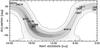 |
Fig. 1 All-sky map (gnomonic projection), showing the mean stellar K-band
flux density distribution of the Milky Way (grayscale, derived from COBE-DIRBE NIR
all-sky maps |

We also re-evaluated the distance estimates toward all globules, confirming the previously- used distances for 7 sources (e.g., Launhardt et al. 2010), and adjusting the distances for 5 sources. CB 4 and CB 6, which we earlier associated with the so-called “−12 km s-1” H I clouds at 600–800 pc, are unlikely to be that far away, as suggested by the lack of foreground stars within a 3′ diameter area toward the cores. Despite their vLSR ~−12 km s-1, they are more likely associated with the Cas A dark clouds in Gould’s Belt at ~350 pc (Perrot & Grenier 2003). CB 68 is associated with the ρ Oph dark clouds, for which we adopt the new precise trigonometric distance of 120 pc from Loinard et al. (2011). B 68 is located within the Pipe nebula and somewhat farther away from ρ Oph. Various direct and indirect estimates suggest a distance of 135 pc ± 15 pc (de Geus et al. 1989; Lombardi et al. 2006; Alves & Franco 2007). For CB 130, which is associated with the Aquila Rift clouds, we adopt the distance estimate of 250 pc ± 50 pc from Straižys et al. (2003).
3. Observations and data reduction
The Herschel FIR continuum data are complemented by submm dust continuum emission maps at 450 μm, 850 μm, and 1.2 mm, obtained with ground-based telescopes. Observations and reduction of both the Herschel and complementary ground-based data are described in the following two subsections. Representative general observing parameters are listed in Table 2, and the observations of individual sources are summarized in Table 3.
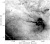 |
Fig. 2 IRAS 100 μm dust continuum emission map, showing the ρ Oph region and the location of two of our target sources (B 68 and CB 68). The plane of the Milky Way is visible at the lower left corner of the map. Compare to Figs. A.7 and C.7. |
3.1. Herschel FIR observations
FIR continuum maps at five wavelength bands were obtained with two different instruments on board the Herschel Space observatory: PACS at 100 and 160 μm, and SPIRE at 250, 350, and 500 μm.
3.1.1. PACS data
All 12 sources were observed with the Herschel Photodetector Array Camera and Spectrometer (PACS; Poglitsch et al. 2010) in the scan map mode at 100 and 160 μm simultaneously. For each source, we obtained two scan directions oriented perpendicular to each other to eliminate striping in the final combined maps of effective size ~10′ × 10′. The scan speed was set to 20″ s-1, and a total of 30 repetitions were obtained in each scan direction, resulting in a total integration time of ~2.6 h per map. We emphasize that the accurate recovery of extended emission is the main driver for the following discussion and exploration of reduction schemes. The PACS data at 100 μm and 160 μm were processed in an identical fashion. They were reduced to level 1 using HIPE v. 6.0.1196 (Ott 2010), except for CB4 (processed with HIPE v. 6.0.2044), CB26 (processed with v. 6.0.2055), and CB6 (processed with v. 7.0.1931).
The rationale for using different versions of HIPE for different sources is that the latter three sources were observed much later (OD 660-770) than the other sources (OD 230-511) and the data were reduced with the respective latest HIPE version and calibration tree available at that time. Since processing of the PACS scanning data is very time-consuming, a re-reduction of all data with every new HIPE version with modifications relevant for our data is not feasible. Instead, we re-reduced the data for one source with the latest version of HIPE to verify how much the data reduction and post-processing modifications affect our results on the derived dust temperature and column density maps. Since this comparison, which is discussed in Sect. 6.1, shows that the effects are well within the range of the other uncertainties, we do not re-reduce all data, but incorporate these effects into our uncertainty assessment in Sect. 6.1.
General observing parameters.
Apart from the standard reduction steps, we applied “2nd level deglitching” to remove outliers in the time series data (“time-ordered” option) by applying a clipping algorithm (based on the median absolute deviation) to all flux measurements in the data stream that will ultimately contribute to the respective map pixel. For our data sets we applied an “nsigma” value of 20.
After producing level 1 data, we generated final level 2 maps using two different methods: high-pass filtering with photproject (within HIPE) and Scanamorphos (Roussel 2012), which does not use straightforward high-pass filtering, but instead applies its own heuristic algorithms to remove artifacts caused by detector flickering noise as well as spurious bolometer temperature drifts. Based on the high-pass median-window subtraction method, the photproject images turned out to suffer from more missing flux and striping than the Scanamorphos images. Because the correct recovery of extended emission is critical for accurate temperature mapping, high-pass filtering is clearly disadvantageous for our science goals. We also note that in a previous reduction, we found that the MADmap4 processing of our brighter sources (e.g., B 335) produces large artifacts5 in the final maps due to the relatively bright central protostar; therefore we do not utilize this reduction scheme in this work.
For these reasons we decided to use Scanamorphos v. 9 as our standard level 2 data
reduction algorithm. A comparison of final maps processed with different Scanamorphos
v. 9 options showed that the “galactic” option recovered the highest
levels of extended emission and was thus the best-suited for our data set and scientific
goals. We use a uniform final map pixel scale of  pix-1 at 100
μm and
pix-1 at 100
μm and  pix-1 at 160
μm for all objects. Furthermore, these data were processed including
the non-zero-acceleration telescope turn-around data, with no additional deglitching
(“noglitch” setting).
pix-1 at 160
μm for all objects. Furthermore, these data were processed including
the non-zero-acceleration telescope turn-around data, with no additional deglitching
(“noglitch” setting).
3.1.2. SPIRE data
All 12 sources were also observed with the Spectral and Photometric Imaging Receiver (SPIRE; Griffin et al. 2010) at 250, 350, and 500 μm. The scan maps of each source were obtained simultaneously at all three bands at the nominal scan speed of 30′′/s and over a (16′−20′)2 area, resulting in a total integration time of 10−16 mins per map. These data were processed up to level 1 with HIPE v. 5.0.1892 and calibration tree 5.1, which was the most up-to-date version at the time all data became available. In Sect. 6.1, we show that using the newest HIPE v. 9.1.0 only leads to nonsignificant minor changes in the SPIRE maps that are well below all other uncertainties. For this reason, we considered it unnecessary to re-reduce the data. Up to level 1 (i.e., the level where the pointed photometer timelines are derived), we performed the steps of the official pipeline (POF5_pipeline.py, dated 2.3.2010) provided by the SPIRE Instrument Control Center (ICC). The level 1 frames were then processed with the Scanamorphos software version 9 (Roussel 2012). All maps were reduced using the “galactic” option. The final map pixel sizes are 6, 10, and 14″ at 250, 350, and 500 μm, respectively.
Photometric color corrections for both PACS and SPIRE data, that account for the difference in spectral slopes between flux calibration (flat spectrum) and actually observed source spectrum, are applied only in the subsequent data analysis and are described in Sect. 4.1.
3.2. (Sub)mm continuum observations
We also use complementary submm dust continuum emission maps at 450 μm, 850 μm, and 1.2 mm from ground-based telescopes for all 12 sources. Part of these complementary data we obtained and published in the past or retrieved from public archives. References to these data are given in Table 3.
Additional dedicated maps of the 1.2 mm dust emission from 6 sources were obtained with the 117-pixel MAMBO-2 bolometer array of the Max-Planck-Institut für Radioastronomie (Kreysa et al. 1999) at the IRAM 30 m-telescope on Pico Veleta (Spain) during two pool observing runs in October and November 2010. The mean frequency (assuming a flat-spectrum source) is 250 GHz (λ0 ~ 1.2 mm) with a half power (HP) bandwidth of ~80 GHz. The HP beam width (HPBW) on sky is 11′′, and the field of view (FoV) of the array is 4′ (20′′ pixel spacing). Weather conditions were good, with zenith optical depths between 0.1 and 0.35 for most of the time and low sky noise. Pointing, focus, and zenith optical depth (by skydip) were measured before and after each map. The pointing stability was better than 3′′ rms. Absolute flux calibration was obtained by observing Uranus several times during the observing runs and monitored by regularly observing several secondary calibrators. The flux calibration uncertainty is dominated by the uncertainty in the knowledge of the planet fluxes and is estimated to be ~20%. The sources were observed with the standard on-the-fly dual-beam technique, with the telescope scanning in azimuth direction at a speed of 8′′/s while chopping with the secondary mirror along the scan direction at a rate of 2 Hz. Most sources were mapped twice, with different projected scanning directions (ideally orthogonal) and different chopper throws (46′′ and 60′′) to minimize scanning artifacts in the final maps. For one source (CB 27), we could obtain only one coverage. Effective map sizes (central pixel coverage) were adapted to the individual source sizes and were in the range 5′–10′, resulting in total mapping times per coverage of 40 min to 1.5 h.
Summary of FIR and submm observations.
The raw data were reduced using the standard pipeline “mapCSF” provided with the MOPSIC software6. Basic reduction steps include de-spiking from cosmic ray artifacts, correlated signal filtering to reduce the skynoise, baseline fitting and subtraction, restoring single-beam maps from the dual-beam scan data using a modified EKH algorithm (Emerson et al. 1979), and transformation and averaging of the individual horizontal maps into the equatorial system. Correlated skynoise correction was performed iteratively, starting with no source model in the first run. The resulting map is smoothed and the region with source flux is selected manually to represent the first source model, which is then iteratively improved in 20 successive correlated skynoise subtraction runs. Since our sources are faint, we follow the recommendation to apply this algorithm only up to level 1, except for the brightest source B335, where we go up to level 3. A third-order polynomial baseline fit to the time-ordered data stream and first-order fits to the individual scan legs are subtracted from the data, after masking out the region with source flux, to correct for slow atmospheric and instrumental drifts. Despite some unsolved electronic problems during these observing runs, which limited the efficiency of the correlated skynoise subtraction, the resulting noise levels in the final maps are ~6 mJy/beam, except for CB 27, where it is ~11 mJy/beam because only one coverage could be obtained.
The assumption of a flat-spectrum source in the definition of the nominal wavelength of the MAMBO detectors in combination with the broad bandpass made it necessary to apply a “color correction”. In contrast to the Herschel FIR observations, (sub)mm wavelengths are sufficiently close to the Rayleigh-Jeans regime and the emission is optically thin for all our sources, such that the slope of the SED follows Sν ∝ λ-4 (for the dust opacity submm spectral index β = 2). Therefore, we follow Schnee et al. (2010) and correct the reference wavelength for all MAMBO data to 1100 μm. Color corrections for the SCUBA data are negligibly small (cf. Schnee et al. 2010) and are not applied.
We also verified the pointing in the final maps by comparing the emission peak positions with interferometric positions where available (CB 26, CB 68, CB 230, CB 244, B 335, BHR 12) and found that deviations are in all cases <2′′, hence confirming the pointing stability and making additional pointing corrections unnecessary. The final maps of those sources for which we had both old and new 1.2 mm data (CB 6, CB 17, CB 26, and CB 230) were generated by weighted averaging, after adapting beam sizes and correcting small pointing offsets.
Additional complementary NIR extinction maps as well as different molecular spectral line maps were also obtained with the aim of studying the relation between density, temperature, and dust properties on the one side, and gas phase abundances and chemistry on the other side. These latter data will be described and analyzed in forthcoming papers and are not presented here.
4. Modeling approach
4.1. Strategy and data preparation
The calibrated dust emission maps at the various wavelengths were used to compile spatially and spectrally resolved data cubes that cover the full extent of these relatively isolated sources on both sides of the peak of their thermal SEDs. Ideally, one would want to compare such data to synthetic maps from radiative transfer models convolved with the respective beams (forward-modeling, virtual observations) to constrain the physical properties of the sources. However, to avoid circular averaging with its well-known caveats, one would need 3D modeling to account for the complex structure present even in these relatively simple and isolated sources. Furthermore, not all of the observed features (like, e.g., the core-envelope temperature contrast, see Sects. 5.6 and 5.7) may be easily reproducible with existing self-consistent models, making the fully self-consistent forward-modeling approach very time-consuming. This will therefore be dealt with in forthcoming papers modeling individual cores.
For this survey overview paper, we take a simpler and more direct approach, giving up some of the spatial information in the short-wavelength maps and directly recovering and modeling beam and LoS optical-depth-averaged (hereafter LOS-averaged for short) SEDs, thus introducing as few as possible model-dependent assumptions into our analysis. For this purpose, the calibrated maps are prepared in the following way:
-
1.
all maps are registered to a common coordinate system;
-
2.
pointing corrections are applied where necessary (see below);
-
3.
all maps are converted to the same physical surface brightness units (here Jy/□′′) and extended emission calibration corrections are applied where necessary (see below);
-
5.
background levels are determined and subtracted from the maps (see below), and finally;
-
6.
all maps are convolved to the SPIRE 500 μm beam (FWHM 36.′′4).
PACS pointing corrections: since the Herschel spacecraft absolute 1σ pointing error was ~2′′ and the PACS and SPIRE maps were not obtained simultaneously, random relative pointing errors between PACS and SPIRE maps can add up to ~3′′–4′′, which is about half the PACS 100 μm FWHM beam size (Aniano et al. 2011). This could severely hamper the usefulness of flux ratio (SED) maps, in particular around compact sources, if not corrected properly. For the long-wavelength SPIRE maps with beam sizes ~18′′–36′′ and no readily available astrometric reference, the pointing errors are fortunately negligible. For the PACS maps we utilize the fact that many 100 μm point sources are also detected in the Spitzer MIPS 24 μm images. We select in each field three stars detected in both the PACS 100 μm and MIPS 24 μm images to align the PACS astrometry in both the 100 μm and 160 μm images to the Spitzer images. The pointing corrections were found to be ≤3′′ in all cases, i.e., small compared to the SPIRE 500 μm beam.
Surface brightness calibration corrections: since the PACS images are calibrated to Jy pix-1, the conversion to Jy/□′′ does not involve an assumption of the beam sizes. The SPIRE data, on the other hand, are calibrated to Jy beam-1; to convert to surface brightness units we adopt the FWHM beam sizes from Aniano et al. (2011) listed in Table 2. The (sub)mm data have also been converted to Jy/□′′ assuming the appropriate effective beam sizes for the respective observations (see references in Table 3). Since the standard calibration is done on point sources, but we are using the surface brightness to compile spatially resolved SEDs, we applied the recommended extended emission calibration corrections to the SPIRE data (see SPIRE Observer’s Manual: HERSCHEL-DOC-0798, version 2.4, June 7, 2011).
PACS and SPIRE map background subtraction: the Scanamor-phos “galactic” option preserves the large spatial frequency modes of the bolometer signal in the Herschel scan-maps. However, the absolute flux level of the background and spatial structures more extended than the scan-maps cannot be recovered since the exact level of the strong thermal background from the only passively cooled mirrors M1 and M2 of the observatory is unknown. Therefore, it is not clear how the extended, large-scale emission levels in the final Herschel maps are related to the absolute flux level of the background, which is composed of emission features larger than the map size, the general Galactic background ISRF, the cosmic microwave background (CMB), and other possible contributions, all varying differently with wavelength. Since uncertainties in additive flux contributions affect flux ratio measurements and the respective derivation of physical parameters from the SEDs, in particular at low flux levels, we subtract the background levels from all Herschel maps, thus making them consistent with the chopped (sub)mm data (although chopping is much more aggressive than the spatial filtering present in the Herschel maps). The consequences and uncertainties of this background removal on the data analysis are discussed in Sects. 4.2 and 6.1. We emphasize that this approach was feasible only because our sources were already initially selected to be relatively isolated on the sky (see Sect. 2).
To accomplish this re-zeroing, we adopt a method similar to that applied to Spitzer MIPS images in Stutz et al. (2009a). For each object we identify a 4′ × 4′ region in the PACS and SPIRE images that is relatively free from spatially varying emission and appears “dark” relative to the globule extended emission levels. We impose the additional requirement that this region is in or near a region in our complementary molecular line maps which is relatively free of 12CO(2–1) emission. We always use the same region in all five Herschel scan-maps. For each band, we then calculate the representative flux level, fDC, in the 4′ × 4′ region by implementing an iterative Gaussian fitting and σ-clipping scheme to the pixel value distribution at each wavelength. We do not consider pixels below 2σ from the mean and fit the main peak of the pixel value distribution. The fDC value is then determined by iteratively fitting a Gaussian function to the histogram of pixel values, where at each iteration we include one more adjacent higher flux bin. The final adopted value of fDC is defined as the mean value of the best-fit Gaussian that has the minimum σ value for all iterations. In this way we exclude pixels with higher flux which effectively broaden the distribution and would cause a bias in the fDC calculation. The fDC values are then subtracted from the corresponding Herschel maps at the respective wavelength (see Table 4 for the fDC and σ values and coordinates of the reference region).
Image convolution: finally, all maps are convolved to the beam of the SPIRE 500 μm map, using the azimuthally averaged Herschel convolution kernels provided by Aniano et al. (2011). For the convolution of the (sub)mm maps, we use a Gaussian convolution kernel of width equal to the difference in quadrature between the effective FWHM of the (sub)mm observations and the SPIRE 500 μm FWHM of 36.′′4.
DC–flux levels in the Herschel data.
After re-gridding to a common Nyquist-sampled pixel grid, we thus compile pixel-by-pixel SEDs for the wavelength range from 100 μm through 1.2 mm. Photometric color corrections for each pixel and each band are iteratively derived from the 100–160 μm and 250–500 μm spectral indices and polynomial fits to color correction factors provided for PACS in Table 2 of Müller et al. (2011) and in Table 5.3 of the SPIRE Observers Manual, and are applied in the subsequent SED modeling only.
The nominal point-source calibration uncertainty of the PACS photometers listed in the latest calibration notes is 3% at 100 μm and 5% at 160 μm. However, additional uncertainites that are hard to quantify are introduced by, e.g., the conversion to surface brightness units for extended emission, the beam convolution (imperfect kernels), and the color corrections. Likewise, the final recommended calibration uncertainty of 7% for SPIRE does not account for some of the uncertainties introduced in the post-processing. Recent systematic comparisons between the Herschel and Spitzer surface brightness calibrations showed that they agree to within about 10%, with intrinsic uncertainties on both sides7. Therefore, we adopt for all Herschel data the conservative value of 15% for the relative calibration uncertainty in the final maps. This number is used for calculating the weights of the individual data points and with respect to the ground-based data in the subsequent fitting procedure (Sect. 4.2).
4.2. Deriving dust temperature and column density maps
The subtraction (or chopping out) of a flat background level from the emission maps
implies that the remaining emission in the map at each image pixel is given by
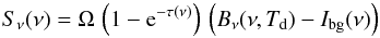 (1)with
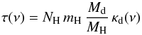 (2)where
Sν(ν) is the observed flux
density at frequency ν, Ω the solid angle from which the flux arises
(here normalized to 1 arcsec2), τ(ν) the
optical depth through the cloud,
Bν(ν,Td)
the Planck function, Td the dust temperature,
Ibg(ν) the background flux level,
NH = 2 × N(H2) + N(H)
the total hydrogen column density, mH the proton mass,
Md/MH the
dust-to-hydrogen mass ratio, and κd(ν) the
dust mass absorption coefficient. Td and
κd may vary along the LoS, in which case Eq. (1) has to be written in differential form and
integrated along the LoS. However, for this overview paper we assume both parameters to be
constant along the LoS and discuss the uncertainties and limitations of this approach in
Sect. 6.2.
(2)where
Sν(ν) is the observed flux
density at frequency ν, Ω the solid angle from which the flux arises
(here normalized to 1 arcsec2), τ(ν) the
optical depth through the cloud,
Bν(ν,Td)
the Planck function, Td the dust temperature,
Ibg(ν) the background flux level,
NH = 2 × N(H2) + N(H)
the total hydrogen column density, mH the proton mass,
Md/MH the
dust-to-hydrogen mass ratio, and κd(ν) the
dust mass absorption coefficient. Td and
κd may vary along the LoS, in which case Eq. (1) has to be written in differential form and
integrated along the LoS. However, for this overview paper we assume both parameters to be
constant along the LoS and discuss the uncertainties and limitations of this approach in
Sect. 6.2.
For κd(ν), we assume for all sources in this paper the tabulated values listed by Ossenkopf & Henning (1994) for mildly coagulated (105 yrs coagulation time at gas density 106 cm-3) composite dust grains with thin ice mantles (Col. 5 in their Table 1, usually called “OH5”), logarithmically interpolated to the respective wavelength where necessary. For the hydrogen-to-dust mass ratio in the Solar neighborhood, we adopt MH/Md = 110 (e.g., Sodroski et al. 1997). Note that the total gas-to-dust mass ratio, accounting for helium and heavy elements, is about 1.36 times higher, i.e., Mg/Md ≈ 150.
The exact background flux levels at the location of the individual clouds, Ibg(ν), are a priori unknown as explained in Sect. 4.1. At the frequencies relevant for this paper, this background radiation is composed mainly of the cmB, the extragalactic cosmic infrared background (CIB), and the diffuse Galactic background (DGB). While the first contribution (CMB) is well-known and dominates at wavelength >500 μm, the mean levels of the CIB have been compiled by, e.g., Hauser & Dwek (2001) from flux measurements in the “Lockman Hole” by various space observatories (e.g., COBE and ISO) and ground-based (sub)mm instruments (e.g., SCUBA). However, at wavelengths <350 μm, the DGB, which strongly varies with position, dominates over cmB and CIB. Here we follow the approach of Stutz et al. (2010) and use the Schlegel et al. (1998) 100 μm IRAS maps and the ISO Serendipity Survey observations at 170 μm to extrapolate approximate mean flux levels at the typical Galactic locations of our sources. Since the uncertainty in the resulting temperature and column density estimates introduced by the uncertainty in the exact knowledge of the Ibg levels is negligible, as discussed quantitatively in Sect. 6.1, we do not attempt to derive the local values of the DGB for each source separately. Instead, we adopt the following mean values for all sources: 0.3, 0.8, 0.5, 0.3, 0.2, 2.9, and 6.5 mJy/arcsec2 at λ 100, 160, 250, 350, 500, 850, and 1100 μm, respectively.
From the calibrated and background-subtracted dust emission maps, we extract for each image pixel the SED with up to 8 data points between 100 μm and 1.2 mm. These individual SEDs are independently fit (χ2 minimization) with a single-temperature modified blackbody of the form of Eqs. (1) and (2) with Td and NH being the free parameters. The individual flux data points are weighted with σ-2, where σ is the quadratic sum of flux times the relative calibration uncertainty (see Sect. 4.1) and the mean rms noise in the respective map measured in regions of zero or lowest emission outside the sources (see Table 4). In order to minimize the effect of T − NH degeneracies in the fitting, because at the low temperatures in these cores, T ≤ 10 K, even the 1.2 mm emission does not represent the Rayleigh-Jeans regime where the SED slope is independent of T, the weight of data points with Sν < σ was set to zero, i.e., these points were not considered in the fitting. To further avoid erroneous extrapolations of the SED fit to unconstrained shorter wavelengths, only pixels with valid fluxes in all 5 Herschel bands were considered. This latter criterion was usually constrained by the PACS 100 μm maps. The best-fitting parameters were derived by employing a least squares fit to all flux values between 100 μm and 1.2 mm at a given image pixel, using a “robust” combination of the classical simplex amoeba search and a modified Levenberg Marquardt method with adaptive steps, as implemented in the “mfit” tool of GILDAS8.
This procedure yields LoS-averaged dust temperature and column density maps of the sources, which are presented in Sect. 5.2. The temperature maps provide a robust estimate of the actual dust temperature of the envelope in the projected outer regions, where the emission is optically thin at all wavelengths and LoS temperature gradients are negligible. Toward the source centers, where cooling and shielding or embedded heating sources can produce significant LoS temperature gradients and the observed SEDs are therefore broader than single-temperature SEDs, the central dust temperatures will be overestimated (in the case of a positive gradient in cold sources) or underestimated (negative gradient in internally heated sources). For these reasons, the column density maps are corrupted and exhibit artifacts in regions of ~20′′–40′′ radius around the warm protostars (see, e.g., Figs. B.7 or B.6). These caveats are discussed and quantified in Sect. 6.2, including some already worked-on solutions.
5. Results
5.1. Herschel FIR maps
The resulting calibrated dust emission maps at λ100, 160, 250, 350, and 500 μm and at original angular resolution are presented in Figs. A.1 through A.12. The Herschel maps are accompanied by optical (red) images from the second Digitized Sky Survey (DSS29), which were obtained through the SkyView10 interface. These optical images clearly show the regions of highest extinction as well as, in several cases, extended cloudshine structures. All maps are overlaid with contours of the (sub)mm dust continuum emission observed with ground-based telescopes.
The 160 through 500 μm maps are usually very similar to each other in appearance, outlining the thermal dust emission from the dense cores along with the often filamentary or tail-like, more tenuous envelopes. Except for some filamentary or tail-like extensions like, e.g., in CB 17 (Fig. A.3), the ~18′ SPIRE maps usually cover the entire extent of the detectable FIR dust emission down to the more or less flat background levels. The slightly smaller PACS maps (~10′) also usually cover the entire extent of the clouds, but in some cases cut off a bit more of some filamentary or tail-like extensions (e.g., Fig. A.3).
The PACS 100 μm maps often show significantly fainter or less extended emission than the maps at longer wavelengths, owing to the fact that 100 μm samples the steep short-wavelength side of the SED at the low temperature of the dust in these clouds (Fig. 4). In some cases, the diffuse 100 μm emission even exhibits a “hole” or “shadow” at the location of the column density peak (e.g., CB 27; Fig. A.5), hinting at extremely cold and dense (high column density) cores with thin warmer envelopes, which are thus good candidates of cores on the verge of protostellar collapse (see Stutz et al. 2009a, for a discussion of 24 μm and 70 μm shadows in dense cores).
On the other hand, the 100 μm maps, which also have the highest angular resolution (≈7′′) of all our Herschel maps, are most sensitive to embedded heating sources like, e.g., protostars. Although even the previously known very low-luminosity object (VeLLO) in CB 130 (Kim et al. 2011; see also Dunham et al. 2008) is well-detected (Fig. A.9), our maps do not reveal any obvious previously unknown warm compact source in any of the globules, confirming that all our presumably starless cores are indeed starless. The only possible exception might be CB 17 (see Fig. A.3), where we find hints of an extremely low-luminosity (Lbol < 0.04 L⊙) cold embedded source very close (in projection) to CB17 - IRS (Chen et al. 2012; Schmalzl et al., in prep.).
5.2. Dust temperature and column density maps and radial profiles
Column density and dust temperature profiles.
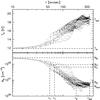 |
Fig. 3 Radial profiles of column density and LoS-averaged dust temperature of B 68 (cf. Fig. 9 of Nielbock et al. 2012 for the ray-tracing results of the same data). Small black dots show the data pixel values over radial distance from the column density peak (see Fig. B.8). Solid gray lines show best fits to these data with Eqs. (3) and (8) and the parameters listed in Table 5. The parameters are also labeled on the diagram axes to illustrate their meaning, with the following characteristic radii: r1 = flat core profile radius (Eq. (3)), r1′ = radius to define consistent dense core boundary (Eqs. (10) and (11)), r2 = cloud radius at transition to halo (Eq. (6)), and rout = outer cloud boundary (Eq. (3)). |
The LoS-averaged dust temperature and hydrogen column density maps derived with the fitting procedure described in Sect. 4.2 are presented in Figs. B.1 through B.12. All sources show systematic dust temperature gradients with cold interiors (11–14 K) and significantly warmer outer rims (14–20 K). Embedded heating sources like protostars, including the VeLLO in CB 130 (Fig. B.9; Kim et al. 2011), show up very clearly in the temperature maps.
To characterize the column density profiles quantitatively, we fit circular profiles
around the column density peak to the maps, using a “Plummer-like” profile (Plummer 1911; see also Whitworth & Ward-Thompson 2001), modified by a constant term to account
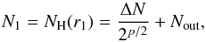
for the observed outer column density “plateau” (see discussion in Sect. 5.7): 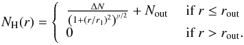 (3)The
peak column density is then
(3)The
peak column density is then  (4)This profile accounts for
an inner flat (column) density core at
r < r1 where
(4)This profile accounts for
an inner flat (column) density core at
r < r1 where
 (5)approaches a power-law
with index p at r ≫ r1,
turns over into a flat outer column density “plateau” outside
(5)approaches a power-law
with index p at r ≫ r1,
turns over into a flat outer column density “plateau” outside 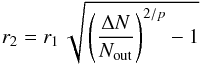 (6)where
 (7)and is cut off at
rout. This outer boundary of the thin envelope or halo is
not well-recovered in most cases because filamentary extensions emphasize deviations from
circular/spherical geometry with increasing distance from the core center and the flux
levels gradually decline below the noise cut-off (see Sect. 4.2). For the same reason, the flatness of the outer column density profile at
level Nout might be partially an artifact of circularly
averaging noncircular structure at a level just above the noise.
(7)and is cut off at
rout. This outer boundary of the thin envelope or halo is
not well-recovered in most cases because filamentary extensions emphasize deviations from
circular/spherical geometry with increasing distance from the core center and the flux
levels gradually decline below the noise cut-off (see Sect. 4.2). For the same reason, the flatness of the outer column density profile at
level Nout might be partially an artifact of circularly
averaging noncircular structure at a level just above the noise.
To empirically fit and parameterize the radial temperature profiles of purely externally
heated cores, we use a similar profile of the form:  (8)The central temperature
minimum is then given by
(8)The central temperature
minimum is then given by  (9)Before fitting
radial profiles to the maps, we mask some of the spurious low-SNR edge features and
tail-like (asymmetric) extensions, always applying the same spatial mask in both the
column density and dust temperature maps. For cores with embedded heating sources
(protostars), we also mask the region with local temperature increase before fitting the
radial profiles with Eqs. (3) and (8) and also list in Table 5 the value of the central temperature maximum
Tpeak. The radius of the masked region varied between
20′′ and 40′′. This extrapolation for
N0 and Tin of the outer profile
into the core center, where both the local temperature and the column density estimates
are very uncertain due to large and unresolved LoS temperature gradients, leads to an
increased uncertainty in particular of the value for N0 in the
protostellar cores. This and other shortcomings of this model and the interpretation of
its parameters are discussed in Sect. 6.2.
(9)Before fitting
radial profiles to the maps, we mask some of the spurious low-SNR edge features and
tail-like (asymmetric) extensions, always applying the same spatial mask in both the
column density and dust temperature maps. For cores with embedded heating sources
(protostars), we also mask the region with local temperature increase before fitting the
radial profiles with Eqs. (3) and (8) and also list in Table 5 the value of the central temperature maximum
Tpeak. The radius of the masked region varied between
20′′ and 40′′. This extrapolation for
N0 and Tin of the outer profile
into the core center, where both the local temperature and the column density estimates
are very uncertain due to large and unresolved LoS temperature gradients, leads to an
increased uncertainty in particular of the value for N0 in the
protostellar cores. This and other shortcomings of this model and the interpretation of
its parameters are discussed in Sect. 6.2.
To illustrate the quality of these radial profile fits and the meaning of the various parameters, we show in Fig. 3 the radial distribution of NH and Td values in the resulting maps for B 68 along with the best-fit profiles and the parameters labeled on the diagram axes. The best-fit parameter values for N0, Nout, r1, r2, rout, p, Tin, Tpeak (for cores with embedded heating sources), and Tout of all sources are listed in Table 5. We do not list parameters rT and q, but note that from the core centers outward, the LoS-averaged dust temperature typically raises by 1 K at a radius of (1 ± 0.3) × 104 AU.
Note that in the next section, we define core and cloud sizes via the mean extent of certain column density contours in the maps, and not via the radial profile fit parameters r1 and rout. In particular for very elliptical sources and sources with extended halos, the derived mean diameters are therefore not necessarily identical to twice the corresponding radial profile-fit radii.
5.3. Source morphologies, integral properties, and SEDs
In addition to the pixel-by-pixel SEDs and the column density and dust temperature maps, we also derive integrated source properties using certain column density levels to define the integration areas. Total cloud sizes are derived by measuring the major and minor extent of the Nout contour in the column density maps, which is marked as the outer yellow contour in Figs. B.1 through B.12. The resulting linear diameters (invoking the distances listed in Table 1) are listed in Table 6. The mean radii of the globules in our sample range from 0.1 pc (CB 130) to 0.5 pc (CB 230), with a mean of 0.22 ± 0.1 pc (4.8 ± 2.2 × 10⁴ AU), which is about twice the typical Jeans lengths of these clouds (≈0.13 pc, assuming the mean radius and mass and a mean temperature of 13 K; see also stability discussion in Sect. 5.5). The mean projected aspect ratio of the clouds is 0.66 ± 0.16, with the most extreme cases CB 6 and BHR 12 (0.4) and B 335 (0.98). These measures do not account for the long tails, e.g., in CB 17 or CB 68, nor do they accurately reflect the actual aspect ratios of the individual sources, since the 3D projection of the elliptical clouds onto the plane of sky remains unknown. Note that these and the following uncertainty values only represent the variance of the mean and do not include systematic uncertainties, which are discussed in Sect. 6.
Since cometary tails in globules appear to be failry ubiquitous (see Table 6 and Sect. 5.8), we have also assessed the possibility that some of the apparently tail-less globules (e.g., B 335 or CB 130) could also have a tail pointing at us or away from us. However, given the length of the tails observed, e.g., in CB 6 (Fig. C.2), CB 17 (Fig. C.3), or CB 68 (Fig. C.7), it is extremely unlikely that a globule like B 335 has a tail that is directly aligned with the line of sight. Another argument against this possibility comes from the fact that, at least in the starless cores, the (LoS-averaged) temperature minimum always agrees with the column density maximum. Should a long tail, like the one seen in e.g., CB 17, be oriented along the line of sight, then its total column density would sum up to a value similar to or even higher than the actually observed ones. However, since the tails are not as well-shielded from the IRSF as spherical cores and therefore have approximately the same average temperature as the envelopes, such a projection could not result in a clear temperature minimum at the position of the column density maximum, as observed in all starless cores.
Physical parameters of globules and embedded cores.
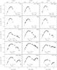 |
Fig. 4 Integrated spectral energy distributions of the dense cores and embedded sources listed in Table 6. Fluxes are integrated within the N1′ contour (Eq. (10)), as are the core masses and luminosities listed in Table 6. Solid lines between 3 mm and 100 μm mark the modified blackbody fits to the data points, while dashed lines only represent a logarithmic interpolation of the data points shortward of 100 μm (see Sect. 5.3). |
Total hydrogen masses are derived by integrating the column density maps within the Nout contour and are also listed in Table 6. These masses range from 0.8 M⊙ (B 335) to 18 M⊙ (CB 230), with a mean value of ⟨ Mcloud ⟩ = 5.4 ± 5.0 M⊙. Using the somewhat more conservative column density threshold N2 (Eq. (7)) would have the benefit of being less susceptible to inhomogeneities of the background level and having closed contours in all sources, but would cut off some of the extended emission that most likely originates from the globule. Using N2 instead of Nout would lead to ≈10–15% lower masses and smaller sizes for the globules compared to the values listed in Table 6.
Integral cloud SEDs (not shown) are obtained by integrating the various emission maps within the Nout contour. Where available and appropriate, we also include ground-based optical and NIR data, Spitzer IRAC and MIPS maps, as well as ISO and IRAS fluxes (see Launhardt et al. 2010). We then fit the resulting SEDs between λ 100 μm and 1.2 mm in the same way as the individual image pixel SEDs (Sect. 4.2). To facilitate integration of the SEDs at wavelengths shortward of the SED peak, fluxes at λ ≤ 100 μm are logarithmically interpolated as described in Launhardt et al. (2010). Bolometric luminosities (Lbol) are derived by integrating the SEDs over the complete wavelength range. Submillimeter luminosities (Lsmm) are derived by integrating the SEDs at wavelengths longward of 350 μm. The resulting total cloud luminosities range from 1.3 L⊙ (CB 17, B 68, B 335) to 29 L⊙ (BHR 12), with a mean of ⟨ Lcloud ⟩ ~ 6.7 L⊙. See Table 6 and Fig. 7 for the distribution of masses and luminosities.
In four out of the twelve globules, the Herschel and submm maps reveal multiple cores (CB 26, BHR 12, CB 130, CB 244 - all known before to be multiple), while the other eight globules appear single-cored at the Herschel resolution. In the temperature and column density maps, the double cores are only resolved clearly in CB 26 and CB 244.
The identification of a common criterion for characterizing the extent and measuring
masses and luminosities of the dense cores was less straight-forward. Since the (column)
density profile of a single-cored globule continuously decreases from the center toward
the outer boundary of the globule, there is no simple way to observationally distinguish
between a “core” and an “envelope”, like in larger molecular clouds where the outer
boundary of a core is usually judged to be where the (column) density profile merges with
the surrounding cloud level. The flat core radius, r1, of the
column density profile is also not a good criterion since its value depends on the derived
power-law index p (Eq. (3)), which is not well-constrained in most cases since
r24r1, i.e., the range where the
column density profile approaches a power-law and p can be derived is too
small in many cases. Therefore, we define an empirical, but well-reproducible column
density threshold for all dense cores by  (10)where e
is Euler’s number and
(10)where e
is Euler’s number and  (11)For
p = 2/ln(2) (~2.9, which is actually very close to the mean
⟨ p ⟩ of our sample), we obtain
N1′ = N1 and
r1′ = r1 (Eq. (5)). This column density threshold is high
enough to permit a reasonable separation of the subcores in CB 26 (Fig. B.4) and CB 244 (Fig. B.12), while at the same time being low enough to fully include the regions of
corrupted column density values around embedded protostars (due to strong unresolved LoS
temperature gradients; cf. Sect. 4.2). Note that
this is an observationally driven definition of “core” that is not based on a
well-characterized physical transition between core and envelope (see also discussion in
Sect. 5.4). In a few cases, we had to use ellipses
to define the core areas, which were however guided by the
N1′ contour. In CB 26 (Fig. B.4), the N1′
contour still includes a bridge between cores SMM1 and SMM2, such that an artifical
cut-off by an ellipse was necessary. In addition, the corruption of the column density map
around SMM1 by unresolved LoS temperature gradients leads to an offset between the column
density peak (artifact) and the temperature peak (actual location of the embedded YSO).
This latter effect required to also use ellipses for CB 244-SMM1 (Fig. B.12) and BHR 12 (Fig. B.6).
(11)For
p = 2/ln(2) (~2.9, which is actually very close to the mean
⟨ p ⟩ of our sample), we obtain
N1′ = N1 and
r1′ = r1 (Eq. (5)). This column density threshold is high
enough to permit a reasonable separation of the subcores in CB 26 (Fig. B.4) and CB 244 (Fig. B.12), while at the same time being low enough to fully include the regions of
corrupted column density values around embedded protostars (due to strong unresolved LoS
temperature gradients; cf. Sect. 4.2). Note that
this is an observationally driven definition of “core” that is not based on a
well-characterized physical transition between core and envelope (see also discussion in
Sect. 5.4). In a few cases, we had to use ellipses
to define the core areas, which were however guided by the
N1′ contour. In CB 26 (Fig. B.4), the N1′
contour still includes a bridge between cores SMM1 and SMM2, such that an artifical
cut-off by an ellipse was necessary. In addition, the corruption of the column density map
around SMM1 by unresolved LoS temperature gradients leads to an offset between the column
density peak (artifact) and the temperature peak (actual location of the embedded YSO).
This latter effect required to also use ellipses for CB 244-SMM1 (Fig. B.12) and BHR 12 (Fig. B.6).
The resulting integral SEDs of the core regions enclosed by the N1′ contours or the respective ellipses (where marked in Figs. B.1 through B.12) are shown in Fig. 4. These SEDs were derived in the same way as described above for the integral cloud SEDs. The integral properties derived from these subregions are much more representative of the cold starless cores or warm protostellar cores than the total globule quantities which include the extended envelopes that are dominated by external heating from the ISRF. Resulting sizes, aspect ratios, masses, and bolometric luminosities of the cores are listed in Table 6. The relation between SEDs and evolutionary stages is discussed in Sect. 5.4.
The mean core diameters, as defined by the N1′ contour and listed in Table 6, range from 8.5 × 10³ AU (0.04 pc; B 335) to 5.2 × 10⁴ AU (0.25 pc; CB 4), with a mean of (2.5 ± 1) × 104 AU (0.12 ± 0.05 pc). The mean aspect ratio of the cores is ⟨ b:a ⟩ = 0.8 ± 0.14, i.e., they are somewhat rounder than the globule envelopes. However, this latter difference is not significant since beam-smoothing does affect the cores more than the envelopes. The mean angular diameter of the cores derived this way is for all sources more than twice as large than the beam (HPBW 36.′′4), and for half of the sources more than three times larger. Hence, the effect of the beam size on the core definition is weak, although not completely negligible in some sources. A more severe limitation on the accuracy of core mass estimates may come from the fact that in the presence of unresolved warm protostars and large LoS temperature gradients, the column density maps are corrupted at the location of the protostar and the peak column density can be underestimated (see Sect. 4.2). In these cases, the core masses are underestimated and the core sizes have larger uncertainties.
The mean total hydrogen mass of all dense cores in our sample is 1.2 ± 0.9 M⊙, with the lowest-mass core being in B 335 (0.2 M⊙), the highest-mass core in BHR 12 (3.7 M⊙), and no significant systematic difference between starless and protostellar cores. The cores in single-core globules contain on average 25 ± 6% of the total mass of the globule, irrespective of whether they already contain a protostar or not. In globules with two cores (CB 26 and CB 244), the total core mass fraction is comparable (30 ± 5%), but the individual cores constitute only 15 ± 6% of the total globule mass. In terms of their luminosity, starless and protostellar cores are more distinct from each other. The mean bolometric luminosity of the seven starless cores (Table 6, including CB 130) is 0.43 ± 0.15 L⊙, while that of the cores with embedded protostars is 4.5 L⊙ with a large scatter ranging from 0.5 L⊙ to 15 L⊙ (excluding CB 17 - IRS). The dense starless cores emit on average 20 ± 5% of the total luminosity of their hosting globules, while protostellar cores emit on average 40 ± 10%. These relations are discussed in more detail and in the context of the thermal structure of the globules and the relative effects of external and internal heating in Sect. 5.6.
5.4. Evolutionary stage tracers
The spectral classes and the approximate evolutionary stages of the sources in our sample were already known from earlier observations and modeling (see Table 1 and Launhardt et al. 2010). With the Herschel data in hand, which provide a much more complete coverage of the thermal SEDs and allow for more robust mass, luminosity, and Tbol estimates than before, we re-evaluate the classical evolutionary tracers Lsmm/Lbol (André et al. 1993) and Tbol (Myers & Ladd 1993). Figure 5 shows the Lsmm/Lbol ratio vs. Tbol for all dense cores in the 12 globules of our sample. Uncertainties of these values are not straigt-forward to assess because the formal error bars are much smaller than the effect of exactly how a core and the respective integration area are defined. Based on tests with slightly different core definitions we estimate the relative uncertainties to be about 10%. In contrast to earlier “pre-Herschel” papers, the new Lsmm/Lbol vs. Tbol diagram now also includes purely externally heated starless cores. At the end of this section, we also use complementary information to relate the empirical “Class” of the individual sources to their actual evolutionary stage.
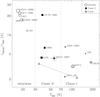 |
Fig. 5 Lbol/Lsubmm ratio vs. bolometric temperature of the globule cores (see Table 6 and Sect. 5.4). The size of the symbols scales with the peak column density of the respective sources. Error bars on CB 244 - SMM1 illustrate the 10% relative uncertainity on both values (Sect. 5.4). The “classical” Tbol boundaries for Class 0 protostars are indicated by the vertical dashed lines. The two triangles, connected by a dotted line, represent one synthetic protostar-envelope system taken from (Robitaille et al. 2006), once seen close to edge-on (Tbol = 34 K) and once seen nearly pole-on into the outflow cavity (Tbol = 119 K; see discussion in Sect. 5.4). |
All starless cores in our sample, i.e., cores that do not have a compact 100 μm source or any other signs of central heating or star formation, have Tbol < 25 K and 10% < Lsmm/Lbol < 30%. We also find a correlation between Tbol and Lsmm/Lbol ratios and both mass and peak column density of starless cores in the sense that colder cores (lower Tbol) with higher Lsmm/Lbol ratios tend to be more massive (see Fig. 5). Since these cores have no significant internal heating sources, this correlation is likely to reflect purely the degree of external heating by the ISRF and shielding rather than an evolutionary effect (see also discussion in Sect. 5.7). Massive cores with higher column densities are better shielded and can cool down more than less-massive and less-shielded cores. Even in the unlikely case that some of these cores would already have undetected first hydrostactic cores (FHSCs), their existence would have no measurable effect on Tbol or the Lsmm/Lbol ratio. Furthermore, an evolution of these integral quantities through the lifetmine of the FHSC is for the same reasons also not expected theoretically (e.g., Commerçon et al. 2012). On the other hand, cores in larger molecular clouds with active star formation may be expected to have both more shielding and a stronger local ISRF, which may lead to different temperature profiles and different location in the Lsmm/Lbol vs. Tbol diagram as compared to isolated cores.
All cores with embedded sources previously classified as Class 0 protostars are confirmed to have 30 K < Tbol < 70 K and and have 3% < Lsmm/Lbol < 7%. The only exception is the core of CB 130 with the embedded VeLLO, which has Lsmm/Lbol ~ 21%. All cores with embedded sources previously classified as Class I YSOs are confirmed to have Tbol > 70 K and have 2% < Lsmm/Lbol < 7%.
While the Lsmm/Lbol ratios we
derive for the isolated Class 0 sources agree well with the upper half of the range of the
values listed by, e.g., André et al. (2000) for
Class 0 sources in larger molecular clouds, we find significantly higher (up to a factor
of 10) Lsmm/Lbol ratios for the
more evolved Class I YSOs than derived and proposed as threshold by André et al. (1993) and André et al.
(2000, Lsmm/ . In fact, we do not find a
significant systematic difference in the
Lsmm/Lbol ratios between Class 0
protostars and Class I YSOs, but see at most a slight trend. As in Launhardt et al. (2010), we argue here that this systematic difference
in Lsmm/Lbol ratios between
isolated and embedded Class I YSOs is unlikely to be an artifact of distance bias, angular
resolution, or SED coverage, but rather reflects a combination of different methods of
identifying the core boundaries and possibly real environmental differences. Luminosities
for these earlier embedded samples were derived by Andre
& Montmerle (1994), Moriarty-Schieven et
al. (1994), and others based on IRAS point source fluxes and ground-based 800 and
1100 μm or 1.3 mm maps only. The compact, warm embedded sources dominate
the small submm maps completely and the remaining low-level emission from a possible
envelope was most likely chopped out to a large extent against the extended emission from
the surrounding cloud (inter-core) material. Hence, these older observations could not
correctly account for the envelope emission. In contrast, the column density profile of a
globule core continuously decreases toward the “edge” of the small cloud, the isolated
envelopes are heated more by the ISRF, and we do have spatially resolved emission maps at
wavelengths between 100 μm and 1.3 mm at hand. The net effect is that we
recover more envelope emission than those earlier observations and the envelopes of the
isolated sources are more luminous than those of the embedded sources, thus elevating the
Lsmm/Lbol ratios.
. In fact, we do not find a
significant systematic difference in the
Lsmm/Lbol ratios between Class 0
protostars and Class I YSOs, but see at most a slight trend. As in Launhardt et al. (2010), we argue here that this systematic difference
in Lsmm/Lbol ratios between
isolated and embedded Class I YSOs is unlikely to be an artifact of distance bias, angular
resolution, or SED coverage, but rather reflects a combination of different methods of
identifying the core boundaries and possibly real environmental differences. Luminosities
for these earlier embedded samples were derived by Andre
& Montmerle (1994), Moriarty-Schieven et
al. (1994), and others based on IRAS point source fluxes and ground-based 800 and
1100 μm or 1.3 mm maps only. The compact, warm embedded sources dominate
the small submm maps completely and the remaining low-level emission from a possible
envelope was most likely chopped out to a large extent against the extended emission from
the surrounding cloud (inter-core) material. Hence, these older observations could not
correctly account for the envelope emission. In contrast, the column density profile of a
globule core continuously decreases toward the “edge” of the small cloud, the isolated
envelopes are heated more by the ISRF, and we do have spatially resolved emission maps at
wavelengths between 100 μm and 1.3 mm at hand. The net effect is that we
recover more envelope emission than those earlier observations and the envelopes of the
isolated sources are more luminous than those of the embedded sources, thus elevating the
Lsmm/Lbol ratios.
When trying to interpret the quantities Tbol and Lsmm/Lbol as evolutionary tracers, one has to keep in mind that, as soon as an outflow starts to open a cavity in the envelope, i.e., already early in the Class 0 collapse phase, the observed SED at wavelengths shortward of the thermal peak at λ ≈ 160 μm becomes highly dependent on the viewing angle (e.g., Whitney et al. 2003; Enoch et al. 2009; Offner et al. 2012). Correspondingly, as long as one does not take into account the full source geometry, but instead simply integrates the observed fluxes over 4 π, quantities derived from the SED also become projection-dependent. To illustrate this, we take one specific synthetic protostar - envelope system from Robitaille et al. (2006, model ID: 3008984) with properties similar to our “Class 0” sources (stellar and envelope mass, luminosity, envelope radius, etc.), and analyze its synthetic SED in the same way as our real sources. This synthetic source is once “observed” close to edge-on (i = 87°, w.r.t. the outflow axis), and once close to pole-on (i = 18°). Although the absolute Lsmm/Lbol ratios derived for this model are systematically somewhat lower than those of our real sources, possibly due to a combination of the simplicity of the specific model and the same physical reasons as discussed above, the Tbol values for the two projections (34 K and 119 K) and the Lsmm/Lbol trend cover the full range of “Class 0” and “Class I” sources (see Fig. 5). Hence, without involving more specific information on the opening angle and orientation of the outflow cavities, e.g., from NIR images and high-resolution molecular line maps, together with radiative transfer modeling, a robust evolutionary classification of sources with Tbol > 30 K just from the SEDs is not possible. Protostars seen pole-on have SEDs that can be very similar to those of more evolved YSOs (“Class I” stage) seen edge-on, i.e., for individual sources there is no clear one-to-one correspondence between spectral Class and evolutionary stage.
For CB 26 - SMM1, we know that it is seen nearly edge-on (Launhardt et al. 2009), i.e., its classification as YSO in the Class I evolutionary stage seems to be robust. BHR 12 is harder to judge since the two sub-cores with misaligned outlows are not resolved in our SED. However, the NIR images also seem to indicate that we are viewing them nearly edge-on (e.g., Hodapp & Ladd 1995). Hence, their classification as YSOs in the Class I evolutionary stage seems also robust. For CB 6 and CB 230, the NIR images suggest that we are at least partially looking into the outflow cones (Launhardt et al. 2010), i.e., they could well be protostars (Class 0 evolutionary stage) seen pole-on.
5.5. Stability of starless cores
We evaluate the total gravitational potential and thermal kinetic energies of the starless cores and compare their central densities with the theoretically predicted maximum stable central density of self-gravitating cores to assess which cores are unstable against gravitational collapse und must therefore be prestellar in nature, and which ones are stable.
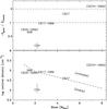 |
Fig. 6 Stability of starless cores. Top: ratio of gravitational potential to thermal kinetic energy vs. total gas mass (1.36 × MH), both integrated within the N2 column density contours (Table 5). The lower dashed horizontal line marks the bounding limit of − Egrav/Etherm = 1, while the upper line marks the state of virialization at − Egrav/Etherm = 2. Bottom: estimated central density (see Sect. 5.5) vs. total gas mass for the same starless cores. The dashed line marks the maximum stable density of a pressure-supported, self-gravitating modified (nonisothermal) BES (with photelectric heating at the core boundary taken into account) as calculated by Keto & Caselli (2008, their Fig. 14). Typical estimated uncertainties on the source parameters are indicated as Y error bars on CB 4. The uncertainty in mass corresponds to the size of the label. |
In a first step, we calculate the gravitational potential energy of the cores as
 (12)with
G being the gravitational constant, and using
R = r2 (Eq. (6) and Table 5),
M = M2 the total gas mass enclosed in the
N2 contour (Eq. (7), mass not explicitely listed here), and the profile shape correction factor
αvir = 0.75(± 0.15) (Bertoldi & McKee 1992; Sipilä et al.
2011). The thermal kinetic energy is calculated as follows:
(12)with
G being the gravitational constant, and using
R = r2 (Eq. (6) and Table 5),
M = M2 the total gas mass enclosed in the
N2 contour (Eq. (7), mass not explicitely listed here), and the profile shape correction factor
αvir = 0.75(± 0.15) (Bertoldi & McKee 1992; Sipilä et al.
2011). The thermal kinetic energy is calculated as follows:  (13)with k
being the Boltzmann constant, μ = 2.33 the mean molecular weight,
mH the proton mass, and
NH × T being integrated within the
N2 contour. Figure 6
(top) shows for the starless cores in our sample the ratio of gravitational to thermal
energy vs. total gas mass M2. The turbulent energy content of
the starless cores (derived from C18O(2–1) line widths; Lippok et al., in
prep.). is by a factor 20–50 lower than the thermal energy for all cores and is thus
negligible in this balance. Given the uncertainties involved in this estimate, this energy
ratio indicates that CB17 - SMM, CB 26 - SMM2, CB 27, and B 68 are all gravitationally
bound and approximately stable. CB244 - SMM2 must be supercritical, which is consistent
with the conclusion derived by Stutz et al.
(2010), and CB 4 does not seem to be gravitationally bound.
(13)with k
being the Boltzmann constant, μ = 2.33 the mean molecular weight,
mH the proton mass, and
NH × T being integrated within the
N2 contour. Figure 6
(top) shows for the starless cores in our sample the ratio of gravitational to thermal
energy vs. total gas mass M2. The turbulent energy content of
the starless cores (derived from C18O(2–1) line widths; Lippok et al., in
prep.). is by a factor 20–50 lower than the thermal energy for all cores and is thus
negligible in this balance. Given the uncertainties involved in this estimate, this energy
ratio indicates that CB17 - SMM, CB 26 - SMM2, CB 27, and B 68 are all gravitationally
bound and approximately stable. CB244 - SMM2 must be supercritical, which is consistent
with the conclusion derived by Stutz et al.
(2010), and CB 4 does not seem to be gravitationally bound.
We also estimate the central volume number density of the starless cores by assuming spherical symmetry and dividing the peak column density N0 by the flat core radius r1 (Eqs. (3), (4) and Table 5) and plot it in Fig. 6 (bottom) against the total gas mass M2. Also indicated in this plot is the maximum stable central density of a pressure-supported, self-gravitating modified (nonisothermal) Bonnor-Ebert sphere (BES; Bonnor 1956; Ebert 1955), calculated by Keto & Caselli (2008, their Fig. 14). For comparison with the isolated globule cores, we adopt their results for the model with photoelectric heating at the core boundary. This evaluation supports the previous conclusions even more clearly, i.e., CB17 - SMM, CB 26 - SMM2, CB 27, and B 68 are all gravitationally bound but seem to be thermally subcritical and just at the limit of stability.
This complies well with the notion that the mean radii of the globules are similar to or only slightly larger than their Jeans lengths (Sect. 5.3). Interestingly, the projected separations between the two sub-cores in CB 26 (0.15 pc) and CB 244 (0.09 pc) agrees quite well with the typical Jeans lengths in these clouds (~0.13 pc; see Sect. 5.3), indicating that large globules tend to fragment gravitationally on the Jeans scale. Also interesting in this respect is that in both globules one of the two cores has already formed a protostar, while the other one is still starless/prestellar.
CB 4 is clearly a subcritical globule and must be purely pressure-confined. CB 244 - SMM2 must be a supercritical prestellar core on the verge of collapse, unless it has significant other nonthermal support like, e.g., strong magnetic fields. The CB 244 region was studied by Wolf et al. (2003) with sub-mm polarization observations. The SMM1 core was indeed found to exhibit a relatively strong magnetic field (257 μG). However, the snr for the SMM2 core was too low to derive a meaningful field strength. Hence, CB 244 - SMM2 is a good candidate to look for kinematic infall signatures or signs of a possibly already existing FHSC.
The finding that the majority of starless cores are bound and approximately stable is a natural consequence of a selection effect. Due to the short collapse time scales (at most 104 yrs, e.g., Schönke & Tscharnuter 2011), unstable cores should be indeed much less frequent than stable cores which can have lifetimes of up to 106 yrs (e.g., Enoch et al. 2008).
5.6. Thermal structure of the cores
Figure 7 shows the bolometric luminosity vs. total hydrogen mass of the entire globules, the dense cores only, and the envelopes only (globule minus core). All globules turn out to have about the same luminosity-to-mass ratio of 1.1 ± 0.6 L⊙/M⊙, irrespective of whether they harbor starless cores or protostars. The mean luminosity-to-mass ratio of the envelopes (cores subracted) is very similar, with somewhat lower scatter (1.0 ± 0.5 L⊙/M⊙). A significant difference in the luminosity-to-mass ratios between starless and protostar-harboring sources exists only for the central dense cores, with starless cores having 0.5 ± 0.25 L⊙/M⊙ and protostellar cores having 2.5 ± 1 L⊙/M⊙. This alone already points toward the dominating effect of the externally heated envelopes for the globules and the very local effect of internal heating by embedded (low-mass) protostars. The embedded protostars have very little effect on the overall energy balance of their host globule.
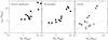 |
Fig. 7 Bolometric luminosity vs. total hydrogen mass of the entire globules (left), the envelopes only (without the dense cores; center) and the dense cores only (right; see Table 6 and Sect. 5.6). Filled quares in the right-most panel mark protostellar cores, empty circels mark starless cores, and the open square marks the core of CB 130 with the embedded VeLLO. |
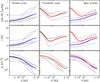 |
Fig. 8 Radially averaged column density profiles (bottom), LoS-averaged dust temperature (center), and luminosity-to-mass ratio profiles (top), for individual sources (thin black solid lines) as well as mean profiles (thick lines) of starless and protostellar cores. Note that the latter ones are fits to the mean profiles, while we list the means of the indivudual profile parameters in Table 5, which is not exactly the same. Thin lines in the rightmost panels indicate the 1σ uncertainty ranges of the mean profiles. |
This dominating effect of external heating and shielding becomes even more evident in the radial profiles of the dust temperature and the local luminosity-to-mass ratios. Figure 8 shows these radial profiles along with the column density profiles for all resolved starless and protostellar cores as well as the mean profiles for these two groups. Both starless globules and globules harboring protostars approach at their outer boundaries, at radii of ~5 × 10⁴ AU and column densities of ~1021 cm-2, dust temperatures of 15.5 ± 1.5 K and local luminosity-to-mass ratios of 2 ± 1 L⊙/M⊙. From the outer boundaries inward, both the dust temperatures and local luminosity-to-mass ratios decrease to reach mean values of 12–13 K and ~0.4 L⊙/M⊙ at radii of ~5000 AU. Hence, all of these cores are far from being isothermal. They are heated externally by the IRSF and their innermost dense centers are well-shielded from the energetic short-wavelength radiation of this heating source. Local heating by the embedded protostars raises the dust temperature and local luminosity-to-mass ratio only inside radii of ~5000 AU, where the derived local temperature is only a lower limit due to the effects of beam-convolution and LoS-averaging. However, there are also some systematic differences between certain globules, which we attribute to differences in the shielding by extended halos and difference in the local ISRF. This is discussed in the next section. Table 5 also lists the column density and temperature profile fit parameters of the mean profiles of protostellar and starless cores in our sample. Note that these mean profile parameters are averages of the individual source profile parameters, while the mean profiles shown in Fig. 8 are derived by fitting the averaged profiles. These observationally derived mean profile parameters can be used to construct representative cores for radiative transfer models. Such models must be able to explain not only the outer and inner dust temperatures, but also the temperature contrast between core and envelope.
5.7. Constraints on the interstellar radiation field
Figure 9 shows the central minimum (LoS-averaged) dust temperature, Tin, of all starless cores in our sample vs. their peak column density N0 (see Table 5). The tight anti-correlation between total column density and central dust temperature indicates very clearly that the inner temperatures of passive molecular cloud cores (without internal heating sources) are controled by the shielding against the ISRF. It also indicates that these nearby and isolated globules are all exposed to about the same ISRF. The correlated errors between Tin and N0 are much smaller than the range of values for these sources and therefore do not affect this conclusion.
We also use the observed outer dust temperatures and halo column densities (Nout) of our sources to derive constraints on the mean ISRF. For this purpose, we compare the observed temperature profiles of the cores in this paper to a grid of 1D radiative transfer models (Shirley et al., in prep.). Dust temperatures are self-consistently calculated using the CSDUST3 code (Egan et al. 1988) for an input density profile, input dust opacities, and input heating conditions. The density profiles are isothermal BES with the BES temperature derived iteratively at the half-central density point of the profile from the radiative transfer calculation. The central densities of the BESs vary from 9 × 103 cm-3 to 6 × 106 cm-3 with the outer radius set to 30 000 AU. The dust opacities are taken from Ossenkopf & Henning (1994, OH5) and are augmented by scattering coefficients according to the prescription given in Young & Evans (2005). The heating is derived from the ISRF plotted in Fig. 3 of Shirley et al. (2005) and is modified in two ways: the overall strength of the UV to FIR ISRF is multiplied by a factor (SISRF), and the model core is assumed to be embedded within a medium with extinction given by AV(Rout) affecting only the shortest wavelengths (λ < few μm) of the ISRF. The final grid consists of 3600 models with self-consistently calculated dust temperature profiles.
Figure 10 compares the modeled relation between the outer temperature (at Rout = 30 000 AU), the relative strengths of the ISRF, and the additional shielding of the cloud against the ISRF by a halo for a model core that matches the mean column density profile of the observed starless globules (Fig. 8) with the observed outer dust temperature and column densities of the outer halos (see Table 5). The observed outer temperatures range from 13.1 K to 19.5 K and occupy the upper half of the model outer temperatures which range from 8.1 K to 17.8 K. The general shape of the observed dependency of the outer temperature on the shielding against the ISRF agrees well with the model calculations, suggesting that the outer temperature is indeed controled to first order by the shielding against an approximately uniform (not necessarily isotropic) ISRF. The only source that deviates significantly from the observed relation toward higher outer temperature or stronger ISRF is BHR 12 (CG 30). This cometary globule in the Gum nebula region is exposed to the Vela pulsar and supernova remnant (Large et al. 1968) and to the O4 supergiant star ζ Puppis, and might thus indeed experience a stronger local ISRF than the other globules (Fig. C.6).
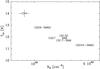 |
Fig. 9 Central minimum (LoS-averaged) dust temperature, Tin, of starless cores vs. peak column density N0. Representative error bars are indicated only for CB 4. |
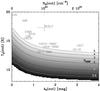 |
Fig. 10 Observed mean outer dust temperatures of the globules vs. column density of the outer halo (see Table 5). The conversion to AV was done with the mean AV-to-NH ratio of (1.5 ± 0.5) × 10-21 derived from the comparison of NIR extinction maps (not used further in this paper) of 9 globules and the NH maps derived in this paper and thus remains somewhat uncertain. Errorbars on BHR12 mark uncertainties of ±0.5 K for Td and 20% for NH (out), repectively. Plotted as grayscale and contours is the dust temperature at the outer radius (30 000 AU) of a model cloud, derived with the radiative transfer modeling descibed in Sect. 5.7, versus shielding of the cloud against the ISRF by a halo and as function of the relative strengths of the ISRF. |
However, the comparison between observations and model calculations also shows that the isolated globules have on average higher outer dust temperatures than predicted by Shirley et al. (2005). This is probably due to a combination of a stronger ISRF than adopted and lower submm opacities for grains with a smaller size distribution than OH5. For this calculation, we used the same dust opacity model for both the dense cold cores and for the thin extended envelopes. OH5 opacities, which are calculated for coagulated dust grains with ice mantles, are certainly not appropriate for the thin extended halos around the globules. Though opacity models for smaller grains will not significantly affect the observational derivation of dust temperatures from the SEDs, they would lead to lower values of the derived outer column densities (by a factor of a few). At the same time, smaller grains would lead to higher outer dust temperatures in the self-consistently calculated models. These issues require further modeling before robust conclusions on the strength of the ISRF can be drawn and will be addressed in a forthcoming paper that will also include information from NIR extinction maps.
Nevertheless, the observed relation between outer dust temperatures and halo column densities complies very well with the general picture of external heating by the ISRF and, at the same time, suggests that our background flux level treatment and extended emission recovery (Sect. 4.1) worked well and that the detected “halos” indeed belong to the globules and do not represent unrelated background material.
5.8. Environmental effects
Although all globules selected for this study appear at first glance compact and not very filamentary, eight out of the 12 globules are cometary-shaped with one sharp rim and either a long cometary tail seen both in the optical cloudshine as well as in the FIR dust emission (e.g. CB 6, CB 17, CB 68), or at least a very diffuse side opposite the sharp rim (e.g., CB 26, CB 230; see Table 6 and Figs. C.1 through C.12). Most of these globules were not classified originally as cometary globules like, e.g., BHR 12 (CG 30; Zealey et al. 1983), but appear at first glance rather round and isolated when seen on less deep optical images or older dust emission maps. The diffuse tails have projected physical lengths between 0.3 pc (CB 27; Fig. C.5) and 2.6 pc (CB 6; Fig. C.2). In some cases, like CB 68, the long diffuse tail connects the globule to larger (diffuse) clouds (Figs. 2 and C.7). In other cases, like BHR 12, the cometary tail is pointing away from an energetic irradiating source (Fig. C.6). In some sources, like CB 17, neither a connection of the long tail to another structure nor an illuminating source could be clearly identified. This diversity suggests that cometary shape and tails may not have the same physical origin in all sources.
We also evaluated the location and orientation of warm rims on the outer edges of the globules (like, e.g., CB 26: Fig. B.4) and their relation to (potential) external heating sources, like nearby stars or the Galactic plane. Even though the one-sided warm rim appears at first glance questionable in some cases because we have recorded no information for the temperature of the opposite rim (e.g., CB 4 and CB 17: Figs. B.1 and B.3), the existence and location of the one-sided warm rims is indeed significant. The warm rims, were present, are on average 2 ± 0.4 K warmer than the opposite cold rims. Their presence can be understood by inspecting the PACS and SPIRE maps of, e.g., CB 4 (Fig. A.1). While the long-wavelength SPIRE maps, which are to first order sensitive to column density, show an approximate symmetry between northern and southern side of the globule (apart from the cometary tail), the shorter-wavelength PACS maps, which are more sensitive to temperature, show a significant asymmetry with much stronger emission on the southern side. Indeed, after fitting the data, the column density contours indicate an approximate symmetry between northern and southern side down to a few times 1020 cm-2 (Fig. B.1). At lower column densities, we can still derive the temperature at the warm southern rim where the short-wavelength PACS emission is sufficiently strong. But on the northern side, the short-wavelength PACS flux densities drop below the detection threshold. Hence, we can no longer reliably derive a temperature for the cold material which is still traced by the SPIRE maps and may have the same column density as the warmer material on the southern side. When allowing the fitting routine to derive temperatures from only three (SPIRE) wavelengths (cf. Sect. 4.2), we obtain a temperature map that fully confirms the above result and rules out a misinterpretation due to a detection bias driven the data reduction. However, these SPIRE-only derived temperature maps are too unreliable and noisy to be used in the analysis of the source structure presented in this paper. Furthermore, the comparison of the results for CB 244 obtained with different versions of the data reduction and calibration pipeline (Sect. 6.1) also show that the extent and location of the warm south-eastern rim in CB 244 (Fig. B.12) remains unaffected by the specific data reduction version or background subtraction level.
Figures C.1 through C.12 show the large-scale morphology and surroundings of all regions studied in this paper, including the schematic indication of the warm rims and the location of potential external illumination sources. We find no clear indication for a general link between the loaction of the warm rim side in a globule and the location of identified potential external heating sources. In some globules, the warm rim points toward the Galactic plane (CB 26, B 68, CB 68, CB 230, CB 244: Figs. C.4, C.8, C.7, C.11, and C.12), in others it points in the opposite direction (CB 4, CB 27, CB 130: Figs. C.1, C.5, and C.9). In CB 6 (Fig. C.2) and CB 17 (Fig. C.3), there are bright nearby stars identified that could be located at the same distance and thus illuminate the globules directly. However, the warm rims do not point toward the potential illuminators. Except for BHR 12, no other nearby heating or illuminating sources could be uniquely identified. However, even in this globule, the tail pointing away from the illuminating source is significantly warmer than the side facing it (Figs. B.6 and C.6). Hence, we have to conclude that, as with the cometary tails, the link between warm rims and illuminating sources or the physical reason for the asymmetric warm rims remains inconclusive and needs to be addressed by future studies.
6. Discussion
6.1. Calibration and data reduction uncertainties
The total flux scale uncertainty of the Herschel data is assumed to be 15% (Sect. 4.1), while that for the ground-based submm bolometer data is about 20% (Sect. 3.2). These flux calibration uncertainties propagate directly into the column density and mass estimates. However, the effect on the dust temperature estimates should be much weaker for the following reason. Since all bands within one of the Herschel instruments were photometrically calibrated in a consistent way, any systematic uncertainties in the effective temperature of the calibrators should be correlated between the bands and thus to first order not affect the flux ratios that determine the temperature. There could still be a systematic offset between PACS and SPIRE due to different calibration procedures. However, if such an offset exists, it would have become immediately evident in the combined pixel-by-pixels SEDs since we have more than one wavelength band from each instrument. Since, after the background offset subtraction (Sect. 4.1), we did not notice any such offset, it must be very small (see also the integrated SEDs in Fig. 4). Similarly, any systematic errors that we could have possibly introduced in the various post-processing steps described in Sect. 4.1 (e.g., spatial filtering) should also be correlated to first order between the Herschel bands. Here we assess these effects quantitatively and estimate the uncertainties introduced by using different and older versions of HIPE and Scanamorphos for different sources (Sect. 3.1). In particular, we reprocessed all Herschel data from one source (CB 244, originally reduced with HIPE v. 5/6 and Scanamorphos v. 9) with the newest versions of HIPE (v. 9) and Scanamorphos (v. 18), with all additional post-processing steps (e.g., background subtraction) unchanged. The new reduction resulted in up to 20% lower PACS fluxes (as compared to the old reduction), but left the SPIRE fluxes unchanged within ≈1%. As a result, the LoS-averaged dust temperatures derived with the newly processed Herschel maps are on average 2.2% lower than the old values, and the resulting column densities are on average 7.5% higher. We also interpret these numbers here as a general assessment of the possible changes that new data reduction versions might bring, since HIPE v. 9.1.0 may not be the “final” version.
The complementary ground-based submm data were obtained independently with different instruments and processed with the respective instrument pipelines. Not only are the calibration uncertainties between the instruments and with respect to Herschel no longer correlated, these data are also much more and in a different way affected by spatial filtering. The sum of these effects would make any results based on simple submm flux ratio maps very susceptible to a number of calibration uncertainites. However, in this paper we use all data in a combined analysis in which the dust temperature estimate is to first order determined by the flux ratios of the Herschel bands, while the column density is to first order determined by the long-wavelength SPIRE bands and the submm data. In order to quantify the effect of the calibration uncertainties on our temperature estimates, we carried out a Monte Carlo test on one pixel in the center of B 68, artificially increasing all Herschel fluxes by 15% and randomly modifying the three individual submm fluxes with an rms of 20% and fitting the SEDs in the same way as we did for the normal analysis. As a result, the mean temperature of that pixel was elevated by 0.2 K from 11.8 K to 12.0 K with an rms scatter of 0.2 K. The mean column density was elevated by 6% with an rms scatter of 10%.
The background subtraction described in Sect. 4.2 could have potentially introduced additional uncertainties. However, since Ibg ≪ Bν(10 K) at all wavelengths for all our sources, thanks to the initial source selection in regions of low background, the difference in the final temperature estimates between considering Ibg or setting Ibg = 0 is ΔT ≤ 0.15 K. The uncertainty introduced by not knowing the exact level of the background, but still subtracting a mean guess of Ibg, is correspondingly smaller, i.e., negligible. We therefore estimate the overall relative 1σ uncertainty introduced by flux calibration and data processing uncertainties to be σT ≈ 3% and σN ≈ 15% (quadratic sums of individual contributions described above).
6.2. Uncertainties and limitations of the modeling approach
Throughout this paper, we used OH5 opacities (Ossenkopf & Henning 1994) for all sources and regions. Although this opacity model seems to be a reasonable assumption for this kind of sources, it is not well-constrained observationally and may not accurately reflect the actual dust properties of the individual objects. Furthermore, a single opacity model may not apply to both the dust in the cold dense cores, where coagulation and ice mantle growth may have affected the effective optical properties of the grains, and that in the thin and warm outer envelopes. Since the data do not provide a direct and unambiguous constraint on the dust opacities (this will be subject of a subsequent paper), we tested the dependency of the temperature and column density estimation on different opacity models and report the results here in the form of an uncertainty discussion. In particular, we test for one source (B 68) how the temperature and column density estimates derived with the following five dust opacity models differ with respect to the use of OH5 opacities: (1) OH1 (MRN size distribution, Mathis et al. 1977); (2) OH8 (coagulated grains like OH5, but with thick ice mantles); (3) Weingartner & Draine (WD01) opacities for RV = 5.5 (Weingartner & Draine 2001; Draine 2003)11; and (4, 5) two pure beta models with β = 1.5 and β = 2.5, normalized to OH5 (which has β ≈ 1.9) at λ = 500 μm. The first three of these models lead to deviations in the derived temperature w.r.t. OH5 of about 4% (0.4 K at 10 K), with the maximum deviation occuring for WD01 in the warm envelope (9% or 1.6 K lower than the 18 K derived with OH5). The two extreme beta models result in ≈10% higher temperatures (w.r.t. OH5) for β = 1.5 or 14−18% lower temperatures for β = 2.5, respectively. Hence, we can safely assume that the systematic uncertainty of the dust temperatures listed in Table 5 and introduced by the uncertainty in the dust opacity model is ΔT ≈ ± 1 K. Since the assumption of ISM-like dust (e.g., OH1), which is probably more appropriate for the envelopes than OH5, leads to a reduction of the derived temperature by only a few per cent (w.r.t. OH5), the LOS-averaged temperature contrast between cores and envelopes could be systematically overestimated by ≈0.5 K, i.e., less than the absolute temperature uncertainty.
The LoS-averaged dust temperature maps presented in this paper provide a robust estimate
of the actual dust temperature only for the envelopes in the projected outer regions,
where the emission is optically thin at all wavelengths and LoS temperature gradients are
negligible. Toward the core centers, where cooling and shielding or embedded heating
sources can produce significant LoS temperature gradients and the observed SEDs are
therefore broader than single-temperature SEDs, the local central dust temperature is
overestimated (in the case of a positive gradient in cold sources) or underestimated
(negative gradient in internally heated sources). E.g., for B 68, where we already derived
a model that accounts for LoS gradients, we derive a local central dust temperature of
 K (Nielbock et al. 2012), which is 3.7 ± 1 K lower
than the LoS-averaged temperature of 11.9 ± 1 K we derive in this survey overview paper.
For CB 17, where the outer dust temperature is lower than in B 68 (Table 5), we derive a local central dust temperature that is
only ≈1 K lower than the LoS-averaged dust temperature derived in this paper (Schmalzl et
al., in prep.). Dust opacity model uncertainties cancel out to first order if we compare
only results obtained with the same opacity curves. Thus, we systematically overestimate
the minimal inner dust temperatures by 1–4 K, underestimate the outer envelope dust
temperature by <0.5 K, and underestimate the temperature contrast
between cold core and envelope by 1−4 K.
K (Nielbock et al. 2012), which is 3.7 ± 1 K lower
than the LoS-averaged temperature of 11.9 ± 1 K we derive in this survey overview paper.
For CB 17, where the outer dust temperature is lower than in B 68 (Table 5), we derive a local central dust temperature that is
only ≈1 K lower than the LoS-averaged dust temperature derived in this paper (Schmalzl et
al., in prep.). Dust opacity model uncertainties cancel out to first order if we compare
only results obtained with the same opacity curves. Thus, we systematically overestimate
the minimal inner dust temperatures by 1–4 K, underestimate the outer envelope dust
temperature by <0.5 K, and underestimate the temperature contrast
between cold core and envelope by 1−4 K.
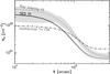 |
Fig. 11 Comparison of radial column density profiles of B 68, derived with the LoS-averaged temperature recovery method described in this paper (black solid line, uncertainty range marked by dotted lines), with the assumption of isothermal dust emission (dash-dotted line), and with a ray-tracing approach that takes LoS temperature gradients into account (gray dashed line, uncertainty range marked by gray-shaded area, Nielbock et al. 2012, corrected for OH5 opacities). |
The effect of systematically overestimating the actual minimum inner dust temperatures on the column density and mass estimates is also not negligible and can be quite significant in individual cases. Figure 11 compares the column density profiles of B 68 derived with an isothermal assumption, the LoS-averaged SED fitting used in this paper, and the full RT approach used in Nielbock et al. (2012). In this rather extreme case (one of the highest core–envelope temperature contrasts in our sample), the LoS-averaged SED fitting underestimates the peak column density by a factor of ≈1.7 and the total mass by ≈15%. In sources with less-pronounced temperature contrast between core and envelope, like CB 17 (Schmalzl et al., in prep.), these systematic effects are weaker. Still, Fig. 11 also illustrates that the column density profiles recovered by our SED fitting approach are a much better approximation to the actual underlying source structure than those derived with an isothermal assumption.
The local temperature minimum and column density peak values are also affected by the angular resolution of our analysis. The 36.′′4 beam size we use for all data may smooth out the central parts of the more centrally peaked profiles in some sources. Although we do not consider this effect being very significant for the starless cores, since the derived flat core radii are all significantly larger than the beam (see Sect. 5.3), it can only be verified quantitatively by using all data in their original resolution and employing full forward modeling. Beam-smoothing does affect the temperature and column density estimates much more at the position of embedded protostars where temperature and density gradients are far more pronounced and definitely not resolved. Here, the local temperatures at the position of embedded protostars are usually strongly underestimated and the temperature and column density maps are often corrupted by even very small residual pointing mismatches.
Hence, we can summarize that the uncertainties introduced by calibration and data reduction issues amount to ≈3% for the temperature and ≈15% for the column density. The uncertainties related to the dust opacity models are significantly larger and amount to ±1 K (≈10%) for the temperature and a factor of up to 3 for the column density and mass. Ignoring LoS temperature gradients leads to an overestimation of the central temperature minima in starless cores by about 1–3 K and an underestimation of the central column density by up to 50%. The temperatures and column densities of the outer envelopes are much less affected by this LoS-averaging.
The largest (systematic) uncertainties of the derived temperatures and (column) densities are clearly related to our uncertain knowledge of the underlying dust mass absorption coefficient and its spectral dependence. Therefore, our goal in future work will be to exploit the Herschel data presented here along with additional complementary data to derive specific observational constraints on the properties of the dust in these globules (see also end of Sect. 7).
6.3. Comparison with earlier observations and models of dense cores
In this section we discuss some examples of previous work based on resolved observations of starless low-mass cores. For comparison with our new Herschel results, we specifically discuss published measurements of density and temperature profiles, as well as different attempts to model said temperature and density profiles.
The observed nonisothermality of dense clouds, derived from Herschel data, was already reported by other authors (e.g., Stutz et al. 2010; Peretto et al. 2010; Battersby et al. 2011; Wilcock et al. 2012; Pitann et al. 2013). While the Stutz et al. (2010) paper was the pilot study for the globule survey presented here, Peretto et al. (2010), Battersby et al. (2011), Wilcock et al. (2012), and Pitann et al. (2013) found that the LoS-averaged dust temperatures in IRDCs also systematically drop toward the highest column densities. Wilcock et al. (2012, Fig. 5) found temperature profiles of IRDCs that are qualitatively very similar to the profiles of the starless globules we report in this paper (Fig. 8), although their outer temperatures are on average ~5 K higher than those found here (20 K vs. 15 K). This is not surprising because IRDCs are generally located in distant regions of high-mass star formation with strong MIR background and may on average be exposed to a stronger ISRF than the nearby isolated globules in the local spiral arm. In more nearby sources, low central temperatures and positive temperature gradients were also inferred from observations and modeling of molecular lines in prestellar cores (e.g., Pagani et al. 2007; Crapsi et al. 2007).
Ward-Thompson et al. (2002) already found observational evidence for temperature gradients and colder interriors of starless cores using flux ratio maps of 170 and 200 μm observed with ISOPHOT. Bacmann et al. (2000) observed 24 dense starless cores in absorption with ISOCAM at 6′′ angular resolution. From modeling of the 7 μm absorption against the MIR background, they derived core structures characterized by a central flat region of Rflat ≈ 4000−8000 AU, central column densities of a few 1022 cm-2, and outer radial column density profiles close to NH ∝ r-1. While the Bacmann et al. (2000) mean peak column densities agree well with the values we derive, our analysis results in somewhat larger flat-core radii and significantly steeper column density profiles (Table 5), which might at least partially be attributable to the larger beam sizes of our maps as compared to the Bacmann work.
Schnee & Goodman (2005) used 450 and 850 μm SCUBA observations to derive the dust temperature profile of the nearby starless core TMC-1C from the 450/850 μm flux ratio (assuming optically thin emission and a fixed β = 1.5). They found a positive temperature gradient with a central dust temperature of 6 K and an outer temperature of 12 K at the edge of the core (at 0.08 pc). They derived similar column densities as we find for the globule sources and modeled the density profile with a broken power-law with a shallow density profile inside ~4000 AU and n ∝ r-1.8 outside. Since the break radius of a broken power-law model of the density is not the same as the parameter r1 of our column density profile fits (Eq. (3)) and should be somewhat smaller, their flat core radius is comparable or slightly smaller (up to a factor of two) than what we derive for the globule cores. Their outer density profile exponent of 1.8 is significantly lower than what would be implied by the column density profiles we derive here (Table 5) and the density profile of B 68 we derive in Nielbock et al. (2012). However, both the dependence of the resulting temperature on the above-mentioned assumptions as well as the nonnegligible calibration uncertainties of the SCUBA data, in particular at 450 μm, make the temperature scale and the (column) density profile derived from such flux ratios rather uncertain.
Shirley et al. (2000) also observed with SCUBA the 450 and 850 μm dust emission of 21 low-mass cores in different evolutionary stages. Based on these observations, Evans et al. (2001) modeled the emission of three starless cores within the context of a self-consistent radiative transfer analysis assuming a nonisothermal BES, modified OH5 dust opacities, and a modified Black (1994) and Draine (1978) ISRF. They found central densities between 105 and 106 cm-3 and required only fractions (0.3–0.6) of the adopted ISRF to reproduce the 450/850 μm flux ratios. They also derived positive temperature gradients with central dust temperatures of 7−8 K and outer temperatures of 12−13 K and found that the ISRF was the dominant heating source in the absence of a nearby star (see also Zucconi et al. 2001). Given the fact that our LoS-averaged dust temperatures overestimate the actual central temperatures by 1−4 K, their derived central temperatures are still 2−3 K lower than what we find here. However, one has to keep in mind that this is based on very low-number statistics and that their three cores are on average denser and more massive than ours. Therefore, this small difference in central temperatures might be real and reflect different source properties. Their outer temperatures, which are not well-constrained by the observations, are also 2−3 K below the observationally well-constrained values we derive. However, without comparing the same sources, it is not possible to verify whether this reflects real differences in the shielding or is the result of the specific assumptions for the dust properties and the strength of the ISRF they made (see also discussion in Sect. 5.7). However, the same remarks apply as made above about the uncertainty of such quantities that are based only on SCUBA flux ratios.
Shirley et al. (2002) modeled the Class 0 cores from the Shirley et al. (2000) sample by including the internal radiation field from the protostar in addition to the heating from the ISRF to reproduce the 450 and 850 μm fluxes. They found that the dust temperature exceeded 20 K only in the inner ≈103 AU, reached ≈10 K at r ≈ 5000−8000 AU, and increased again slightly toward the outer boundary of the core at a few 104 AU. This is consistent with what we find, including the temperature rise at r > 104 AU, taking again into account that we overestimate the inner minimum temperature by up to 3 K, and that their models appear to underestimate the outer temperatures by 2−3 K.
Stamatellos et al. (2005) calculated temperature profiles in the context of an evolutionary model, starting with a 5.4 M⊙ BES and assuming OH5 dust opacities and a modified Black (1994) ISRF. In the initial stage, when only the ISRF heats the core, they found a central temperature of ~7 K and outer temperatures of up to ~20 K. Stamatellos et al. (2007) further studied the influence of external heating and shielding on the temperature profile of cores in the ρ Oph cloud, taking into account also the surrounding molecular cloud extinction. They found again that the inner core temperatures (at r < 104 AU) are always below 10 K, but derived rim temperatures (at r ≈ 2 × 10⁴ AU) of only ~13–15 K. They noted that in Taurus, where the ambient radiation field is weaker, the core temperatures are found to be somewhat lower with a central value of ≈7 K and rim temperature of ≈12 K for TMC-1C. These temperatures and temperature contrasts are again consistent with what we now measure from the Herschel data in similar cores. In particular the outer temperatures we measure for the isolated globules with their thin halos are all in between the values these authors derived for the unshielded and the well-shielded cores.
7. Summary and conclusions
We study the thermal dust emission from 12 nearby isolated globules using FIR dust continuum maps at five wavelength bands between 100 and 500 μm obtained with the Herschel satellite and submm continuum maps at up to three wavelengths beween 450 μm and 1.2 mm obtained with ground-based telescopes. Great care is taken in both the selection of truly isolated and previously well-characterized sources in regions of exceptionally low background emission and in restoring and calibrating all maps in a consistent manner to enable a combined in-depth analysis of all data. This careful preselection, data treatment, and the very deep 100 μm maps (~50 μJy/arcsec2 rms) are essential to enable our analysis method and lead to the results presented here.
We calibrate all data to the same flux scale, subtract all general background levels in a constistent way, convolve all maps to the same angular resolution, assign weights to each pixel according to calibration uncertainties and rms noise, and extract full SEDs from 100 μm to 1.2 mm for each image pixel. These individual SEDs are independently fit (least squares) with single-temperature modified blackbody curves, using OH5 opacities for mildy coagulated dust grains with thin ice mantles. Thus, we obtain for each image pixel a column density and an LoS-averaged dust temperature. The resulting dust temperature maps have rms noise levels of only a few tenth of a K and systematic uncertainties of less than ±1 K. We then analyze the dust temperature and column density maps along with the integrated SEDs of all sources, including additional archival data at shorter wavelengths, and obtain the following main results:
-
1.
The globules in our sample have a mean distance from the Sun of240 ± 100 pc, mean total gas mass of 7.3 ± 6.8 M⊙, meanbolometric luminosity of ≈6.7 L⊙, and mean outerdiameter of 0.45 ± 0.2 pc. Typical peak column densities(averaged over the 36.′′4 beam) are ⟨ NH ⟩ ≈ 3 × 1022 cm-2, whichcorresponds to peak visual extinctions of about45 mag.
-
2.
The dense cores of the globules have a mean total gas mass of 1.6 ± 1.2 M⊙ and a mean diameter of 0.12 ± 0.05 pc. They constitute on average 25 ± 6% of the total globule mass.
-
3.
Out of the 12 globules in our sample, four contain one starless core each, six contain a protostellar core (Class 0 or I), and two globules contain each one starless and one protostellar core.
-
4.
We confirm the earlier classifications of protostars and embedded YSOs, but the better-sampled thermal SEDs do not allow for better evolutionary stage determination from the SEDs alone since projection effects dominate the spectral appearance of even Class 0 protostars. However, the Herschel data allow us now to also include starless cores in the Lsmm/Lbol vs. Tbol diagram (Fig. 5). We find that all starless cores have Tbol < 25 K and 10% < Lsmm/Lbol < 30%. In particular the criterion Tbol < 25 K can be used to identify isolated and externally heated starless cores, since even an embedded VeLLO will elevate Tbol above 30 K.
-
5.
Most globules are surrounded by a thin (AV ≈ 1−3 mag) and warm (Td ≈ 15–20 K) outer halo, the full extent of which we could not properly recover in most cases. These halos are evident in the dust emission-based column density maps, NIR extinction maps, as well as in many cases on optical images as cloudshine.
-
6.
The thermal structure of all globules is dominated by external heating through the ISRF, with warm outer envelopes (15.5 ± 1.8 K) and colder interiors (<13 ± 1 K). We find a very tight anti-correlation between the minimal central temperatures in starless cores and the total column density toward the outer edge that provides shielding against the ISRF (Fig. 9).
-
7.
The outer dust temperature of the globules is to first order determined by external heating from an approximately uniform ISRF and shielding by thin extended halos. We find a clear anti-correlation between the outer dust temperatures and the mean column density/AV of the halos (Fig. 10). Only one of the globules is exposed to a significantly higher than average local ISRF (BHR 12).
-
8.
The embedded (low-mass and low-luminosity) protostars raise the local temperature of the dense cores only within radii out to about 5000 AU, but do not significantly affect the overall thermal balance of the globules.
-
9.
Our LoS-averaged dust temperatures are accurate to about ±1 K at the outer boundaries of the globules (accounting for both statistical and systematic errors), but systematically overestimate the local central temperature minima by 1–4 K, depending on the temperature contrast to the outer rim. Thus, these globules have central dust temperatures in the range 8–12 K and temperature contrasts to the outer rim of 3–8 K. Note that the gas temperature is expected to be closely coupled to the dust temperature only in the central dense cores, but is likely decoupled and can be significantly higher toward the outer rim where the gas density drops well below 104−105 cm-3.
-
10.
Out of the six starless cores in our sample, five cores are found to be thermally stabilized against gravitational collapse. Of these, four cores (CB 17 - SMM, CB 26 - SMM2, CB 27, and B 68) have central densities that are very close to the maximum stable density of a pressure-supported, self-gravitating cloud, i.e., we cannot distinguish wheter they are starless stable or prestellar. CB 4 is thermally sub-critical and must be a purely pressure-confined starless core. The starless core in CB 244 - SMM2 is clearly super-critical and should very likely be a prestellar core on the verge of collapse.
-
11.
The radius of the single-core globules is very similar to or only slightly larger than their Jeans length (~0.13 pc). The projected core separation in the two double-core globules agrees well with the Jeans lengths in these clouds, indicating that large globules tend to fragment gravitationally on the Jeans scale.
-
12.
Many of the globules have one side that is signifcantly warmer than the other side at the outer rim. Although in some cases the warm side faces the direction toward the Galactic plane, we could not identify a consistent relation between warm side and potential external illuminating sources.
As a next step, we are currently analyzing individual starless cores by employing a ray-tracing algorithm that is able to restore LoS temperature gradients and derive the actual volume density structure of the cores by starting from a 1D model and allowing for local deviations from spherical symmetry (Nielbock et al. 2012; Schmalzl et al., in prep.). This way we hope to better and most robustly constrain the dust temperature structure of these cores without introducing too many model-dependent assumptions into the analysis. We are also working toward better constraining the dust opacity models. For this purpose, we have already obtained deep NIR extinction maps that recover the same angular resolution as the Herschel data and are currently obtaining additional deep submm and mm continuum maps. We are planning to employ and compare different approaches, including SED fitting and ray-tracing like in this paper and in Nielbock et al. (2012), self-consistent radiative transfer modeling like in Shirley et al. (2011), as well as Bayesian approaches like in Kelly et al. (2012). Furthermore, we are currently also using complementary molecular line data to derive constraints on the distribution of turbulence and molecular gas-phase freeze-out onto dust grains in the sources studied in this paper (Lippok et al., in prep.).
Online material
Appendix A: Dust temperature and column density maps
These figures are described and discussed in Sect. 5.2.
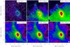 |
Fig. A.1 CB 4 (starless core): visual (red) DSS2 image and Herschel FIR maps (color; log scale) at 100, 160, 250, 350, and 500 μm, with 1.2 mm continuum contours overlaid (20 and 40 mJy/30′′ beam). Herschel beam sizes are indicated as gray circles in the lower right corners. |
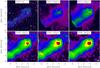 |
Fig. A.2 CB 6 (Class I YSO): visual (red) DSS2 image and Herschel FIR maps (color; log scale) at 100, 160, 250, 350, and 500 μm, with 850 μm continuum contours overlaid (180 and 300 mJy/20′′ beam). Herschel beam sizes are indicated as gray circles in the lower right corners. |
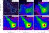 |
Fig. A.3 CB 17 (starless core and embedded Class I YSO): visual (red) DSS2 image and Herschel FIR maps (color; log scale) at 100, 160, 250, 350, and 500 μm, with 1.2 mm continuum contours overlaid (20, 40, and 65 mJy/20′′ beam). Herschel beam sizes are indicated as gray circles in the lower right corners. |
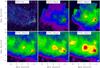 |
Fig. A.4 CB 26 (starless core and embedded Class I YSO): visual (red) DSS2 image and Herschel FIR maps (color; log scale) at 100, 160, 250, 350, and 500 μm, with 1.2 mm continuum contours overlaid (10, 26, and 150 mJy/30′′ beam). Herschel beam sizes are indicated as gray circles in the lower right corners. |
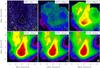 |
Fig. A.5 CB 27 (starless core): visual (red) DSS1 image and Herschel FIR maps (color; log scale) at 100, 160, 250, 350, and 500 μm, with 1.2 mm continuum contours overlaid (40 and 70 mJy/30′′ beam). Herschel beam sizes are indicated as gray circles in the lower right corners. |
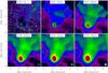 |
Fig. A.6 BHR 12 (Class 0/I protostars): visual (red) DSS2 image and Herschel FIR maps (color; log scale) at 100, 160, 250, 350, and 500 μm, with 850 μm continuum contours overlaid (SCUBA; 120, 300, and 900 mJy/15′′ beam). Herschel beam sizes are indicated as gray circles in the lower right corners. |
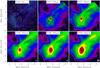 |
Fig. A.7 CB 68 (Class 0 protostar): visual (red) DSS2 image and Herschel FIR maps (color; log scale) at 100, 160, 250, 350, and 500 μm, with 850 μm continuum contours overlaid (150, 300, and 600 mJy/20′′ beam). Herschel beam sizes are indicated as gray circles in the lower right corners. |
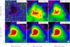 |
Fig. A.8 B 68 (starless core): visual (red) DSS2 image and Herschel FIR maps (color; log scale) at 100, 160, 250, 350, and 500 μm, with 870 μm continuum contours overlaid (40, 120, and 220 mJy/27′′ beam). Herschel beam sizes are indicated as gray circles in the lower right corners. |
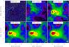 |
Fig. A.9 CB 130 (Class 0 protostar): visual (red) DSS2 image and Herschel FIR maps (color; log scale) at 100, 160, 250, 350, and 500 μm, with 1.2 mm continuum contours overlaid (20, 60, and 100 mJy/20′′ beam). Herschel beam sizes are indicated as gray circles in the lower right corners. |
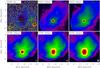 |
Fig. A.10 B 335 (Class 0 protostar): visual (red) DSS2 image and Herschel FIR maps (color; log scale) at 100, 160, 250, 350, and 500 μm, with 850 μm continuum contours overlaid (100, 300, and 900 mJy/20′′ beam). Herschel beam sizes are indicated as gray circles in the lower right corners. |
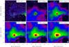 |
Fig. A.11 CB 230 (Class I YSO): visual (red) DSS2 image and Herschel FIR maps (color; log scale) at 100, 160, 250, 350, and 500 μm, with 850 μm continuum contours overlaid (70, 200, and 700 mJy/20′′ beam). Herschel beam sizes are indicated as gray circles in the lower right corners. |
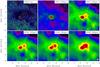 |
Fig. A.12 CB 244 (Class 0 protostar and starless core): Visual (red) DSS2 image and Herschel FIR maps (color; log scale) at 100, 160, 250, 350, and 500 μm, with 1.2 mm continuum contours overlaid (30, 80, and 180 mJy/20′′ beam). Herschel beam sizes are indicated as gray circles in the lower right corners. |
Appendix B: Dust emission maps
These dust emission maps are described in Sect. 5.1.
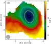 |
Fig. B.1 Dust temperature map of CB 4 (color scale), overlaid with contours of the hydrogen column density (white: 1021 cm-2, black: 0.2, 0.5, 2, and 4 × 1021 cm-2). Yellow contours mark Nout (Eq. (3)) and N1′ (Eq. (10)). The yellow square marks the column density peak and the reference position listed in Table 5. |
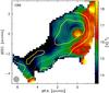 |
Fig. B.2 Dust temperature map of CB 6 (color scale), overlaid with contours of the hydrogen column density (white: 1021 cm-2, black: 2, 4, and 6 × 1021 cm-2). Yellow contours mark Nout (Eq. (3)) and N1′ (Eq. (10)). The dotted yellow ellipse marks the N1′ approximation described in Sect. 5.3. The asterisk marks the position of the embedded YSO. |
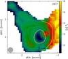 |
Fig. B.3 Dust temperature map of CB 17 (color scale), overlaid with contours of the hydrogen column density (white: 1021 – masked by the yellow Nout contour – and 1022 cm-2, black: 2, 4, 6, 8, and 20 × 1021 cm-2). Yellow contours mark Nout (Eq. (3)) and N1′ (Eq. (10)). The yellow square marks the column density peak and position of CB 17-SMM. The asterisk marks the position of CB 17-IRS (Table 5; see also Launhardt et al. 2010). |
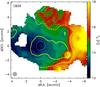 |
Fig. B.4 Dust temperature map of CB 26 (color scale), overlaid with contours of the hydrogen column density (white: 1021 and 1022 cm-2, black: 0.5, 2, 4, 6, and 8 × 1021 cm-2). Yellow contours mark Nout (Eq. (3)) and N1′ (Eq. (10), referring to the starless core SMM2). Dotted yellow ellipses mark the N1′ approximations for the two subcores described in Sect. 5.3. The yellow square marks the column density peak and position of CB 26-SMM2; the asterisk marks the position of CB 26-SMM1 (Table 5). |
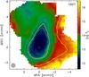 |
Fig. B.5 Dust temperature map of CB 27 (color scale), overlaid with contours of the hydrogen column density (white: 1021 and 1022 cm-2, black: 2, 4, 6, and 8 × 1021 cm-2). Yellow contours mark Nout (Eq. (3)) and N1′ (Eq. (10)). The yellow square marks the column density peak and the reference position listed in Table 5. |
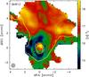 |
Fig. B.6 Dust temperature map of BHR 12 (color scale), overlaid with contours of the hydrogen column density (white: 1021 – masked by yellow Nout contour – and 1022 cm-2, black: 0.5, 2, 4, 6, 8, and 20 × 1021 cm-2). Yellow contours mark Nout (Eq. (3)) and N1′ (Eq. (10)). The dotted yellow ellipse marks the N1′ approximation described in Sect. 5.3. The two asterisks mark the positions of embedded sources SMM1 and SMM2 (see Launhardt et al. 2010). |
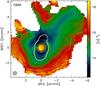 |
Fig. B.7 Dust temperature map of CB 68 (color scale), overlaid with contours of the hydrogen column density (white: 1021 and 1022 cm-2, black: 0.5 – masked by yellow Nout contour – 2, 4, 6, 8, and 20 × 1021 cm-2). Yellow contours mark Nout (Eq. (3)) and N1′ (Eq. (10)). The dotted yellow ellipse marks the N1′ approximation described in Sect. 5.3. The asterisk marks the position of the protostar and the reference position listed in Table 5. |
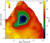 |
Fig. B.8 Dust temperature map of B 68 (color scale), overlaid with contours of the hydrogen column density (white: 1021 and 1022 cm-2, black: 0.5, 2, 4, 6, 8 and 20 × 1021 cm-2). Yellow contours mark Nout (Eq. (3)) and N1′ (Eq. (10)). The yellow square marks the column density peak and the reference position listed in Table 5. |
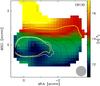 |
Fig. B.9 Dust temperature map of CB 130 (color scale), overlaid with contours of the hydrogen column density (white: 1021 and 1022 cm-2, black: 0.5, 2 – masked by yellow Nout contour – 4, 6, 8, and 20 × 1021 cm-2). Yellow contours mark Nout (Eq. (3)) and N1′ (Eq. (10)). The yellow circle marks the position of the protostellar core CB 130-SMM1 with the embedded Class 0 VeLLO. The yellow square marks the position of the secondary starless core CB 130-SMM2. The asterisk marks the position of the Class I-II YSO CB 130-IRS, which most likely associated with CB 130, but not embedded in its dense core (see Launhardt et al. 2010). |
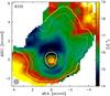 |
Fig. B.10 Dust temperature map of B 335 (color scale), overlaid with contours of the hydrogen column density (white: 1021 and 1022 cm-2, black: 0.5, 2, 4, 6, 8, and 20 × 1021 cm-2). Yellow contours mark Nout (Eq. (3)) and N1′ (Eq. (10)). The asterisk marks the position of the protostar and the reference position listed in Table 5. |
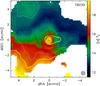 |
Fig. B.11 Dust temperature map of CB 230 (color scale), overlaid with contours of the hydrogen column density (white: 1021 and 1022 cm-2, black: 2, 4, 6, 8, and 20 × 1021 cm-2). Yellow contours mark Nout (Eq. (3)) and N1′ (Eq. (10)). The two asterisks mark the positions of the embedded YSOs (see Launhardt et al. 2010). |
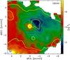 |
Fig. B.12 Dust temperature map of CB 244 (color scale), overlaid with contours of the hydrogen column density (white: 1021 and 1022 cm-2, black: 0.5, 2, 4, 6, 8, and 20 × 1021 cm-2). Yellow contours mark Nout (Eq. (3)) and N1′ (Eq. (10)) for the starless core CB 244-SMM2. The dotted yellow ellipse marks the N1′ approximation for CB244-SMM1 described in Sect. 5.3. The yellow square marks the column density peak of CB 244-SMM2 and the reference position listed in Table 5. The asterisk marks the position of of the protostar CB244-SMM1. |
Appendix C: Images on large-scale morphology
These optical images on the larger-scale morphology of the globules are discussed in Sect. 5.8.
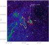 |
Fig. C.1 CB 4: visual (red) DSS2 image with SPIRE 500 μm continuum contours overlaid. The red arc marks the warm rim of CB 4. |
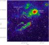 |
Fig. C.2 CB 6: visual (red) DSS2 image with SPIRE 500 μm continuum contours overlaid. The red arc marks the warm rim of CB 6. |
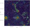 |
Fig. C.3 CB 17: visual (red) DSS2 image with SPIRE 500 μm continuum contours overlaid. The red arc marks the warm rim of CB 17. |
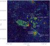 |
Fig. C.4 CB 26: visual (red) DSS2 image with SPIRE 500 μm continuum contours overlaid. The red arc marks the warm rim of CB 26. |
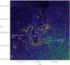 |
Fig. C.5 CB 27: visual (red) DSS1 image with SPIRE 500 μm continuum contours overlaid. The red arc marks the warm rim of CB 27. |
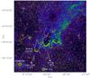 |
Fig. C.6 BHR 12: visual (red) DSS2 image with SPIRE 500 μm continuum contours overlaid. The tail side is warmer than the head side, but there is nor clear warm rim side. |
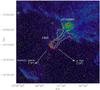 |
Fig. C.7 CB 68: visual (red) DSS2 image with SPIRE 500 μm continuum contours overlaid. The red arc marks the warm rim of CB 68. |
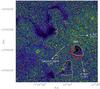 |
Fig. C.8 B 68: visual (red) DSS1 image with SPIRE 500 μm continuum contours overlaid. The red arc marks the warm rim of B 68. The B2 IV star Θ Oph is located at a distance from the Sun of 134 pc, i.e., its physical distance from B 68 is only ≈2.8 pc. |
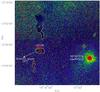 |
Fig. C.9 CB 130: visual (red) DSS2 image with SPIRE 500 μm continuum contours overlaid. The red arc marks the warm rim of CB 130. |
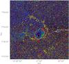 |
Fig. C.10 B 335: visual (red) DSS2 image with SPIRE 500 μm continuum contours overlaid. The red arc marks the warm rim of B 335. |
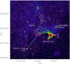 |
Fig. C.11 CB 230: visual (red) DSS2 image with SPIRE 500 μm continuum contours overlaid. The red arc marks the warm rim of CB 230. |
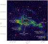 |
Fig. C.12 CB 244: visual (red) DSS2 image with SPIRE 500 μm continuum contours overlaid. The red arc marks the warm rim of CB 244. |
The peak of the flux density of a blackbody with T = 10−20 K is at λ ≈ 290−145 μm. The peak of the energy density (ν Sν) of the optically thin globules at these temperatures is at only slightly shorter wavelengths (230−130 μm).
We use the term “prestellar” only for those starless cores that have been shown to be gravitationally unstable or on the verge of collapse.
This problem has eventually been solved in the most recent MADmap implementation.
Created and continuously updated by Zylka, IRAM, Grenoble; see http://www.iram.es/IRAMES/mainWiki/CookbookMopsic
See PICC-NHSC-TR-034 and PICC-NHSC-TN-029 under https://nhscsci.ipac.caltech.edu/
The Digitized Sky Surveys were produced at the Space Telescope Science Institute under US Government grant NAG W-2166. The images of these surveys are based on photographic data obtained using the Oschin Schmidt Telescope on Palomar Mountain and the UK Schmidt Telescope. The plates were processed into the present compressed digital form with the permission of these institutions.
SkyView has been developed with generous support from the NASA AISR and ADP programs (P.I. Thomas A. McGlynn) under the auspices of the High Energy Astrophysics Science Archive Research Center (HEASARC) at the NASA/ GSFC Astrophysics Science Division.
Acknowledgments
The authors gratefully acknowledge the valuable help from Hélène Roussel in the production of Scanamorphos PACS and SPIRE maps as well as Gonzalo Aniano’s assistance and careful work with the Herschel convolution kernels used in this work. We greatly benefitted from discussions with Yaroslav Pavlyuchenkov (Moscow) on the data analysis. We also thank the anonymous referee for comments and suggestions that helped to improve the clarity and completeness of the paper. Part of this work was supported by the German Deutsche Forschungsgemeinschaft, DFG project number Ts 17/2–1. This publication makes use of data products from the Two Micron All Sky Survey, which is a joint project of the University of Massachusetts and the Infrared Processing and Analysis Center/California Institute of Technology, funded by the National Aeronautics and Space Administration and the National Science Foundation. The work of A.M.S., S.R., and J.K. was supported by the Deutsche Forschungsgemeinschaft priority program 1573 (“Physics of the Interstellar Medium”). H.L., M.N., and Z.B. are supported by Deutsches Zentrum für Luft- und Raumfahrt (DLR).
References
- Agladze, N. I., Sievers, A. J., Jones, S. A., Burlitch, J. M., & Beckwith, S. V. W. 1996, ApJ, 462, 1026 [NASA ADS] [CrossRef] [Google Scholar]
- Alves, F. O., & Franco, G. A. P. 2007, A&A, 470, 597 [NASA ADS] [CrossRef] [EDP Sciences] [Google Scholar]
- Alves, J. F., Lada, C. J., & Lada, E. A. 2001, Nature, 409, 159 [NASA ADS] [CrossRef] [PubMed] [Google Scholar]
- Andre, P., & Montmerle, T. 1994, ApJ, 420, 837 [NASA ADS] [CrossRef] [Google Scholar]
- Andre, P., Ward-Thompson, D., & Barsony, M. 1993, ApJ, 406, 122 [NASA ADS] [CrossRef] [Google Scholar]
- Andre, P., Ward-Thompson, D., & Barsony, M. 2000, Protostars and Planets IV, 59 [Google Scholar]
- André, P., Bouwman, J., Belloche, A., & Hennebelle, P. 2004, Ap&SS, 292, 325 [NASA ADS] [CrossRef] [Google Scholar]
- Aniano, G., Draine, B. T., Gordon, K. D., & Sandstrom, K. 2011, PASP, 123, 1218 [NASA ADS] [CrossRef] [Google Scholar]
- Bacmann, A., André, P., Puget, J.-L., et al. 2000, A&A, 361, 555 [Google Scholar]
- Battersby, C., Bally, J., Ginsburg, A., et al. 2011, A&A, 535, A128 [NASA ADS] [CrossRef] [EDP Sciences] [Google Scholar]
- Bergin, E. A., & Langer, W. D. 1997, ApJ, 486, 316 [NASA ADS] [CrossRef] [Google Scholar]
- Bergin, E. A., & Tafalla, M. 2007, ARA&A, 45, 339 [NASA ADS] [CrossRef] [Google Scholar]
- Bertoldi, F., & McKee, C. F. 1992, ApJ, 395, 140 [NASA ADS] [CrossRef] [Google Scholar]
- Beuther, H., Henning, T., Linz, H., et al. 2010, A&A, 518, L78 [NASA ADS] [CrossRef] [EDP Sciences] [Google Scholar]
- Beuther, H., Tackenberg, J., Linz, H., et al. 2012, A&A, 538, A11 [NASA ADS] [CrossRef] [EDP Sciences] [Google Scholar]
- Bianchi, S., Gonçalves, J., Albrecht, M., et al. 2003, A&A, 399, L43 [NASA ADS] [CrossRef] [EDP Sciences] [Google Scholar]
- Black, J. H. 1994, in The First Symposium on the Infrared Cirrus and Diffuse Interstellar Clouds, 58, 355 [Google Scholar]
- Bonnor, W. B. 1956, MNRAS, 116, 351 [CrossRef] [Google Scholar]
- Boudet, N., Mutschke, H., Nayral, C., et al. 2005, ApJ, 633, 272 [NASA ADS] [CrossRef] [Google Scholar]
- Bourke, T. L., Hyland, A. R., Robinson, G., James, S. D., & Wright, C. M. 1995, MNRAS, 276, 1067 [NASA ADS] [Google Scholar]
- Burton, M. G. 1992, Aust. J. Phys., 45, 463 [Google Scholar]
- Caselli, P., Walmsley, C. M., Tafalla, M., Dore, L., & Myers, P. C. 1999, ApJ, 523, L165 [NASA ADS] [CrossRef] [Google Scholar]
- Caselli, P., Walmsley, C. M., Zucconi, A., et al. 2002, ApJ, 565, 344 [NASA ADS] [CrossRef] [Google Scholar]
- Charnley, S. B. 1997, MNRAS, 291, 455 [NASA ADS] [CrossRef] [Google Scholar]
- Chen, X., Arce, H. G., Dunham, M. M., et al. 2012, ApJ, 751, 89 [NASA ADS] [CrossRef] [Google Scholar]
- Commerçon, B., Hennebelle, P., Audit, E., Chabrier, G., & Teyssier, R. 2010, A&A, 510, L3 [NASA ADS] [CrossRef] [EDP Sciences] [Google Scholar]
- Commerçon, B., Launhardt, R., Dullemond, C. P., & Henning, T. 2012, A&A, 545, A98 [NASA ADS] [CrossRef] [EDP Sciences] [Google Scholar]
- Crapsi, A., Caselli, P., Walmsley, M. C., & Tafalla, M. 2007, A&A, 470, 221 [NASA ADS] [CrossRef] [EDP Sciences] [Google Scholar]
- Draine, B. T. 1978, ApJS, 36, 595 [NASA ADS] [CrossRef] [Google Scholar]
- Draine, B. T. 2003, ARA&A, 41, 241 [NASA ADS] [CrossRef] [Google Scholar]
- Dunham, M. M., Crapsi, A., Evans, N. J., II, et al. 2008, ApJS, 179, 249 [NASA ADS] [CrossRef] [Google Scholar]
- Ebert, R. 1955, Z. Astrophys., 37, 217 [Google Scholar]
- Egan, M. P., Leung, C. M., & Spagna, G. F., Jr. 1988, Comput. Phys. Comm., 48, 271 [Google Scholar]
- Enoch, M. L., Evans, N. J., II, Sargent, A. I., & Glenn, J. 2009, ApJ, 692, 973 [NASA ADS] [CrossRef] [Google Scholar]
- Foster, J. B., & Goodman, A. A. 2006, ApJ, 636, L105 [NASA ADS] [CrossRef] [Google Scholar]
- Di Francesco, J., Evans, N. J., II, Caselli, P., et al. 2007, Protostars and Planets V, 17 [Google Scholar]
- Di Francesco, J., Johnstone, D., Kirk, H., MacKenzie, T., & Ledwosinska, E. 2008, ApJS, 175, 277 [NASA ADS] [CrossRef] [Google Scholar]
- Evans, N. J., II, Rawlings, J. M. C., Shirley, Y. L., & Mundy, L. G. 2001, ApJ, 557, 193 [NASA ADS] [CrossRef] [Google Scholar]
- Emerson, D. T., Klein, U., & Haslam, C. G. T. 1979, A&A, 76, 92 [NASA ADS] [Google Scholar]
- Enoch, M. L., Evans, N. J., II, Sargent, A. I., et al. 2008, ApJ, 684, 1240 [NASA ADS] [CrossRef] [Google Scholar]
- de Geus, E. J., de Zeeuw, P. T., & Lub, J. 1989, A&A, 216, 44 [NASA ADS] [Google Scholar]
- Griffin, M. J., Abergel, A., Abreu, A., et al. 2010, A&A, 518, L3 [Google Scholar]
- Hauser, M. G., & Dwek, E. 2001, ARA&A, 39, 249 [NASA ADS] [CrossRef] [Google Scholar]
- Henning, T., & Launhardt, R. 1998, A&A, 338, 223 [NASA ADS] [Google Scholar]
- Henning, T., & Stognienko, R. 1996, A&A, 311, 291 [NASA ADS] [Google Scholar]
- Henning, T., Linz, H., Krause, O., et al. 2010, A&A, 518, L95 [NASA ADS] [CrossRef] [EDP Sciences] [Google Scholar]
- Hily-Blant, P., Walmsley, M., Pineau Des Forêts, G., & Flower, D. 2010, A&A, 513, A41 [NASA ADS] [CrossRef] [EDP Sciences] [Google Scholar]
- Hodapp, K.-W., & Ladd, E. F. 1995, ApJ, 453, 715 [NASA ADS] [CrossRef] [Google Scholar]
- Juvela, M., Pelkonen, V.-M., Padoan, P., & Mattila, K. 2006, A&A, 457, 877 [NASA ADS] [CrossRef] [EDP Sciences] [Google Scholar]
- Kainulainen, J., Lehtinen, K., & Harju, J. 2006, A&A, 447, 597 [NASA ADS] [CrossRef] [EDP Sciences] [Google Scholar]
- Kainulainen, J., Beuther, H., Henning, T., & Plume, R. 2009, A&A, 508, L35 [NASA ADS] [CrossRef] [EDP Sciences] [Google Scholar]
- Kandori, R., Nakajima, Y., Tamura, M., et al. 2005, AJ, 130, 2166 [NASA ADS] [CrossRef] [Google Scholar]
- Kauffmann, J., Bertoldi, F., Bourke, T. L., Evans, N. J., II, & Lee, C. W. 2008, A&A, 487, 993 [NASA ADS] [CrossRef] [EDP Sciences] [Google Scholar]
- Kelly, B. C., Shetty, R., Stutz, A. M., et al. 2012, ApJ, 752, 55 [NASA ADS] [CrossRef] [Google Scholar]
- Keto, E., & Caselli, P. 2008, ApJ, 683, 238 [NASA ADS] [CrossRef] [Google Scholar]
- Kim, H. J., Evans, N. J., II, Dunham, M. M., et al. 2011, ApJ, 729, 84 [NASA ADS] [CrossRef] [Google Scholar]
- Kirk, J. M., Ward-Thompson, D., & André, P. 2005, MNRAS, 360, 1506 [NASA ADS] [CrossRef] [Google Scholar]
- Kiss, C., Klaas, U., & Lemke, D. 2005, A&A, 430, 343 [NASA ADS] [CrossRef] [EDP Sciences] [Google Scholar]
- Kreysa, E., Gemünd, H.-P., Gromke, J., et al. 1999, Infrared Phys. Technol., 40, 191 [NASA ADS] [CrossRef] [EDP Sciences] [Google Scholar]
- Kun, M. 1998, ApJS, 115, 59 [NASA ADS] [CrossRef] [Google Scholar]
- Lada, C. J., Lada, E. A., Clemens, D. P., & Bally, J. 1994, ApJ, 429, 694 [NASA ADS] [CrossRef] [Google Scholar]
- Lada, C. J., Huard, T. L., Crews, L. J., & Alves, J. F. 2004, ApJ, 610, 303 [NASA ADS] [CrossRef] [Google Scholar]
- Large, M. I., Vaughan, A. E., & Mills, B. Y. 1968, Nature, 220, 340 [NASA ADS] [CrossRef] [Google Scholar]
- Larson, R. B. 1969, MNRAS, 145, 271 [NASA ADS] [CrossRef] [Google Scholar]
- Launhardt, R., & Henning, T. 1997, A&A, 326, 329 [NASA ADS] [Google Scholar]
- Launhardt, R., & Sargent, A. I. 2001, ApJ, 562, L173 [NASA ADS] [CrossRef] [Google Scholar]
- Launhardt, R., Ward-Thompson, D., & Henning, T. 1997, MNRAS, 288, L45 [NASA ADS] [CrossRef] [Google Scholar]
- Launhardt, R., Pavlyuchenkov, Y., Gueth, F., et al. 2009, A&A, 494, 147 [NASA ADS] [CrossRef] [EDP Sciences] [Google Scholar]
- Launhardt, R., Nutter, D., Ward-Thompson, D., et al. 2010, ApJS, 188, 139 [NASA ADS] [CrossRef] [Google Scholar]
- Linz, H., Krause, O., Beuther, H., et al. 2010, A&A, 518, L123 [NASA ADS] [CrossRef] [EDP Sciences] [Google Scholar]
- Loinard, L., Mioduszewski, A. J., Torres, R. M., et al. 2011, Rev. Mex. Astron. Astrofis. Conf. Ser., 40, 205 [NASA ADS] [Google Scholar]
- Lombardi, M., Alves, J., & Lada, C. J. 2006, A&A, 454, 781 [NASA ADS] [CrossRef] [EDP Sciences] [Google Scholar]
- Mathis, J. S., Rumpl, W., & Nordsieck, K. H. 1977, ApJ, 217, 425 [NASA ADS] [CrossRef] [Google Scholar]
- Moriarty-Schieven, G. H., Wannier, P. G., Keene, J., & Tamura, M. 1994, ApJ, 436, 800 [NASA ADS] [CrossRef] [Google Scholar]
- Myers, P. C., & Ladd, E. F. 1993, ApJ, 413, L47 [NASA ADS] [CrossRef] [Google Scholar]
- Motte, F., & André, P. 2001, A&A, 365, 440 [NASA ADS] [CrossRef] [EDP Sciences] [Google Scholar]
- Müller, T., Okumura, K, & Klaas, U. 2011, PACS Photometer Passbands and Colour Correction Factors for Various Source SEDs [Google Scholar]
- Negrello, M., Magliocchetti, M., Moscardini, L., et al. 2004, MNRAS, 352, 493 [NASA ADS] [CrossRef] [Google Scholar]
- Nielbock, M., Launhardt, R., Steinacker, J., et al. 2012, A&A, 547, A11 [NASA ADS] [CrossRef] [EDP Sciences] [Google Scholar]
- Nutter, D., Stamatellos, D., & Ward-Thompson, D. 2009, MNRAS, 396, 1851 [NASA ADS] [CrossRef] [Google Scholar]
- Offner, S. S. R., Robitaille, T. P., Hansen, C. E., McKee, C. F., & Klein, R. I. 2012, ApJ, 753, 98 [NASA ADS] [CrossRef] [Google Scholar]
- Olofsson, S., & Olofsson, G. 2009, A&A, 498, 455 [NASA ADS] [CrossRef] [EDP Sciences] [Google Scholar]
- Ossenkopf, V., & Henning, T. 1994, A&A, 291, 943 [NASA ADS] [Google Scholar]
- Ott, S. 2010, in ADASS XIX, ASP Conf. Ser., 434, 139 [Google Scholar]
- Padoan, P., Juvela, M., & Pelkonen, V.-M. 2006, ApJ, 636, L101 [NASA ADS] [CrossRef] [Google Scholar]
- Pagani, L., Bacmann, A., Cabrit, S., & Vastel, C. 2007, A&A, 467, 179 [NASA ADS] [CrossRef] [EDP Sciences] [Google Scholar]
- Pagani, L., Steinacker, J., Bacmann, A., Stutz, A., & Henning, T. 2010, Science, 329, 1622 [NASA ADS] [CrossRef] [PubMed] [Google Scholar]
- Pavlyuchenkov, Y., Wiebe, D., Launhardt, R., & Henning, T. 2006, ApJ, 645, 1212 [NASA ADS] [CrossRef] [Google Scholar]
- Pavlyuchenkov, Y. N., Wiebe, D. S., Akimkin, V. V., Khramtsova, M. S., & Henning, T. 2012, MNRAS, 421, 2430 [NASA ADS] [CrossRef] [Google Scholar]
- Penston, M. V. 1969, MNRAS, 144, 425 [NASA ADS] [CrossRef] [Google Scholar]
- Peretto, N., Fuller, G. A., Plume, R., et al. 2010, A&A, 518, L98 [NASA ADS] [CrossRef] [EDP Sciences] [Google Scholar]
- Perrot, C. A., & Grenier, I. A. 2003, A&A, 404, 519 [NASA ADS] [CrossRef] [EDP Sciences] [Google Scholar]
- Pilbratt, G. L., Riedinger, J. R., Passvogel, T., et al. 2010, A&A, 518, L1 [CrossRef] [EDP Sciences] [Google Scholar]
- Pitann, J., Linz, H., Ragan, S., et al. 2013, ApJ, accepted [arXiv:1301.1163] [Google Scholar]
- Plummer, H. C. 1911, MNRAS, 71, 460 [CrossRef] [Google Scholar]
- Poglitsch, A., Waelkens, C., Geis, N., et al. 2010, A&A, 518, L2 [NASA ADS] [CrossRef] [EDP Sciences] [Google Scholar]
- Ragan, S., Henning, T., Krause, O., et al. 2012, A&A, 547, A49 [NASA ADS] [CrossRef] [EDP Sciences] [Google Scholar]
- Robitaille, T. P., Whitney, B. A., Indebetouw, R., Wood, K., & Denzmore, P. 2006, ApJS, 167, 256 [NASA ADS] [CrossRef] [Google Scholar]
- Roussel, H. 2012 [arXiv:1205.2576] [Google Scholar]
- Saraceno, P., Andre, P., Ceccarelli, C., Griffin, M., & Molinari, S. 1996, A&A, 309, 827 [NASA ADS] [Google Scholar]
- Sauter, J., Wolf, S., Launhardt, R., et al. 2009, A&A, 505, 1167 [NASA ADS] [CrossRef] [EDP Sciences] [Google Scholar]
- Schlegel, D. J., Finkbeiner, D. P., & Davis, M. 1998, ApJ, 500, 525 [NASA ADS] [CrossRef] [Google Scholar]
- Schnee, S., & Goodman, A. 2005, ApJ, 624, 254 [NASA ADS] [CrossRef] [Google Scholar]
- Schnee, S., Enoch, M., Noriega-Crespo, A., et al. 2010, ApJ, 708, 127 [Google Scholar]
- Schönke, J., & Tscharnuter, W. M. 2011, A&A, 526, A139 [NASA ADS] [CrossRef] [EDP Sciences] [Google Scholar]
- Shetty, R., Kauffmann, J., Schnee, S., Goodman, A. A., & Ercolano, B. 2009a, ApJ, 696, 2234 [NASA ADS] [CrossRef] [Google Scholar]
- Shetty, R., Kauffmann, J., Schnee, S., & Goodman, A. A. 2009b, ApJ, 696, 676 [NASA ADS] [CrossRef] [Google Scholar]
- Shirley, Y. L., Evans, N. J., II, Rawlings, J. M. C., & Gregersen, E. M. 2000, ApJS, 131, 249 [NASA ADS] [CrossRef] [Google Scholar]
- Shirley, Y. L., Evans, N. J., II, & Rawlings, J. M. C. 2002, ApJ, 575, 337 [NASA ADS] [CrossRef] [Google Scholar]
- Shirley, Y. L., Nordhaus, M. K., Grcevich, J. M., et al. 2005, ApJ, 632, 982 [NASA ADS] [CrossRef] [Google Scholar]
- Shirley, Y. L., Huard, T. L., Pontoppidan, K. M., et al. 2011, ApJ, 728, 143 [NASA ADS] [CrossRef] [Google Scholar]
- Shu, F. H. 1977, ApJ, 214, 488 [NASA ADS] [CrossRef] [Google Scholar]
- Shu, F. H., Adams, F. C., & Lizano, S. 1987, ARA&A, 25, 23 [Google Scholar]
- Siebenmorgen, R., Kruegel, E., & Mathis, J. S. 1992, A&A, 266, 501 [NASA ADS] [Google Scholar]
- Sipilä, O., Harju, J., & Juvela, M. 2011, A&A, 535, A49 [NASA ADS] [CrossRef] [EDP Sciences] [Google Scholar]
- Smith, J., Werner, M. W., Lynch, D. K., & Cudaback, D. 1979, ApJ, 234, 902 [NASA ADS] [CrossRef] [Google Scholar]
- Sodroski, T. J., Odegard, N., Arendt, R. G., et al. 1997, ApJ, 480, 173 [NASA ADS] [CrossRef] [Google Scholar]
- Stamatellos, D., Whitworth, A. P., Boyd, D. F. A., & Goodwin, S. P. 2005, A&A, 439, 159 [NASA ADS] [CrossRef] [EDP Sciences] [Google Scholar]
- Stamatellos, D., Whitworth, A. P., & Ward-Thompson, D. 2007, MNRAS, 379, 1390 [NASA ADS] [CrossRef] [Google Scholar]
- Stecklum, B., Launhardt, R., Fischer, O., et al. 2004, ApJ, 617, 418 [NASA ADS] [CrossRef] [Google Scholar]
- Steinacker, J., Pagani, L., Bacmann, A., & Guieu, S. 2010, A&A, 511, A9 [NASA ADS] [CrossRef] [EDP Sciences] [Google Scholar]
- Straižys, V., Černis, K., & Bartašiūtė, S. 2003, A&A, 405, 585 [NASA ADS] [CrossRef] [EDP Sciences] [Google Scholar]
- Stutz, A. M., Rubin, M., Werner, M. W., et al. 2008, ApJ, 687, 389 [NASA ADS] [CrossRef] [Google Scholar]
- Stutz, A. M., Rieke, G. H., Bieging, J. H., et al. 2009a, ApJ, 707, 137 [NASA ADS] [CrossRef] [Google Scholar]
- Stutz, A. M., Bourke, T. L., Rieke, G. H., et al. 2009b, ApJ, 690, L35 [NASA ADS] [CrossRef] [Google Scholar]
- Stutz, A., Launhardt, R., Linz, H., et al. 2010, A&A, 518, L87 [NASA ADS] [CrossRef] [EDP Sciences] [Google Scholar]
- Tobin, J. J., Hartmann, L., Looney, L. W., & Chiang, H.-F. 2010, ApJ, 712, 1010 [NASA ADS] [CrossRef] [Google Scholar]
- Ward-Thompson, D., Scott, P. F., Hills, R. E., & Andre, P. 1994, MNRAS, 268, 276 [NASA ADS] [CrossRef] [Google Scholar]
- Ward-Thompson, D., Motte, F., & Andre, P. 1999, MNRAS, 305, 143 [NASA ADS] [CrossRef] [Google Scholar]
- Ward-Thompson, D., André, P., & Kirk, J. M. 2002, MNRAS, 329, 257 [NASA ADS] [CrossRef] [Google Scholar]
- Weingartner, J. C., & Draine, B. T. 2001, ApJ, 548, 296 [NASA ADS] [CrossRef] [Google Scholar]
- Whitney, B. A., Wood, K., Bjorkman, J. E., & Wolff, M. J. 2003, ApJ, 591, 1049 [Google Scholar]
- Whitworth, A. P., & Ward-Thompson, D. 2001, ApJ, 547, 317 [NASA ADS] [CrossRef] [Google Scholar]
- Wilcock, L. A., Ward-Thompson, D., Kirk, J. M., et al. 2012, MNRAS, 424, 716 [NASA ADS] [CrossRef] [Google Scholar]
- Wolf, S., Launhardt, R., & Henning, T. 2003, ApJ, 592, 233 [NASA ADS] [CrossRef] [Google Scholar]
- Young, C. H., & Evans, N. J., II 2005, ApJ, 627, 293 [NASA ADS] [CrossRef] [Google Scholar]
- Young, C. H., Shirley, Y. L., Evans, N. J., II, & Rawlings, J. M. C. 2003, ApJS, 145, 111 [NASA ADS] [CrossRef] [Google Scholar]
- Zealey, W. J., Ninkov, Z., Rice, E., Hartley, M., & Tritton, S. B. 1983, Astrophys. Lett., 23, 119 [NASA ADS] [Google Scholar]
- Zucconi, A., Walmsley, C. M., & Galli, D. 2001, A&A, 376, 650 [NASA ADS] [CrossRef] [EDP Sciences] [Google Scholar]
All Tables
All Figures
|
Fig. 1 All-sky map (gnomonic projection), showing the mean stellar K-band
flux density distribution of the Milky Way (grayscale, derived from COBE-DIRBE NIR
all-sky maps |
| In the text | |
|
Fig. 2 IRAS 100 μm dust continuum emission map, showing the ρ Oph region and the location of two of our target sources (B 68 and CB 68). The plane of the Milky Way is visible at the lower left corner of the map. Compare to Figs. A.7 and C.7. |
| In the text | |
|
Fig. 3 Radial profiles of column density and LoS-averaged dust temperature of B 68 (cf. Fig. 9 of Nielbock et al. 2012 for the ray-tracing results of the same data). Small black dots show the data pixel values over radial distance from the column density peak (see Fig. B.8). Solid gray lines show best fits to these data with Eqs. (3) and (8) and the parameters listed in Table 5. The parameters are also labeled on the diagram axes to illustrate their meaning, with the following characteristic radii: r1 = flat core profile radius (Eq. (3)), r1′ = radius to define consistent dense core boundary (Eqs. (10) and (11)), r2 = cloud radius at transition to halo (Eq. (6)), and rout = outer cloud boundary (Eq. (3)). |
| In the text | |
|
Fig. 4 Integrated spectral energy distributions of the dense cores and embedded sources listed in Table 6. Fluxes are integrated within the N1′ contour (Eq. (10)), as are the core masses and luminosities listed in Table 6. Solid lines between 3 mm and 100 μm mark the modified blackbody fits to the data points, while dashed lines only represent a logarithmic interpolation of the data points shortward of 100 μm (see Sect. 5.3). |
| In the text | |
|
Fig. 5 Lbol/Lsubmm ratio vs. bolometric temperature of the globule cores (see Table 6 and Sect. 5.4). The size of the symbols scales with the peak column density of the respective sources. Error bars on CB 244 - SMM1 illustrate the 10% relative uncertainity on both values (Sect. 5.4). The “classical” Tbol boundaries for Class 0 protostars are indicated by the vertical dashed lines. The two triangles, connected by a dotted line, represent one synthetic protostar-envelope system taken from (Robitaille et al. 2006), once seen close to edge-on (Tbol = 34 K) and once seen nearly pole-on into the outflow cavity (Tbol = 119 K; see discussion in Sect. 5.4). |
| In the text | |
|
Fig. 6 Stability of starless cores. Top: ratio of gravitational potential to thermal kinetic energy vs. total gas mass (1.36 × MH), both integrated within the N2 column density contours (Table 5). The lower dashed horizontal line marks the bounding limit of − Egrav/Etherm = 1, while the upper line marks the state of virialization at − Egrav/Etherm = 2. Bottom: estimated central density (see Sect. 5.5) vs. total gas mass for the same starless cores. The dashed line marks the maximum stable density of a pressure-supported, self-gravitating modified (nonisothermal) BES (with photelectric heating at the core boundary taken into account) as calculated by Keto & Caselli (2008, their Fig. 14). Typical estimated uncertainties on the source parameters are indicated as Y error bars on CB 4. The uncertainty in mass corresponds to the size of the label. |
| In the text | |
|
Fig. 7 Bolometric luminosity vs. total hydrogen mass of the entire globules (left), the envelopes only (without the dense cores; center) and the dense cores only (right; see Table 6 and Sect. 5.6). Filled quares in the right-most panel mark protostellar cores, empty circels mark starless cores, and the open square marks the core of CB 130 with the embedded VeLLO. |
| In the text | |
|
Fig. 8 Radially averaged column density profiles (bottom), LoS-averaged dust temperature (center), and luminosity-to-mass ratio profiles (top), for individual sources (thin black solid lines) as well as mean profiles (thick lines) of starless and protostellar cores. Note that the latter ones are fits to the mean profiles, while we list the means of the indivudual profile parameters in Table 5, which is not exactly the same. Thin lines in the rightmost panels indicate the 1σ uncertainty ranges of the mean profiles. |
| In the text | |
|
Fig. 9 Central minimum (LoS-averaged) dust temperature, Tin, of starless cores vs. peak column density N0. Representative error bars are indicated only for CB 4. |
| In the text | |
|
Fig. 10 Observed mean outer dust temperatures of the globules vs. column density of the outer halo (see Table 5). The conversion to AV was done with the mean AV-to-NH ratio of (1.5 ± 0.5) × 10-21 derived from the comparison of NIR extinction maps (not used further in this paper) of 9 globules and the NH maps derived in this paper and thus remains somewhat uncertain. Errorbars on BHR12 mark uncertainties of ±0.5 K for Td and 20% for NH (out), repectively. Plotted as grayscale and contours is the dust temperature at the outer radius (30 000 AU) of a model cloud, derived with the radiative transfer modeling descibed in Sect. 5.7, versus shielding of the cloud against the ISRF by a halo and as function of the relative strengths of the ISRF. |
| In the text | |
|
Fig. 11 Comparison of radial column density profiles of B 68, derived with the LoS-averaged temperature recovery method described in this paper (black solid line, uncertainty range marked by dotted lines), with the assumption of isothermal dust emission (dash-dotted line), and with a ray-tracing approach that takes LoS temperature gradients into account (gray dashed line, uncertainty range marked by gray-shaded area, Nielbock et al. 2012, corrected for OH5 opacities). |
| In the text | |
|
Fig. A.1 CB 4 (starless core): visual (red) DSS2 image and Herschel FIR maps (color; log scale) at 100, 160, 250, 350, and 500 μm, with 1.2 mm continuum contours overlaid (20 and 40 mJy/30′′ beam). Herschel beam sizes are indicated as gray circles in the lower right corners. |
| In the text | |
|
Fig. A.2 CB 6 (Class I YSO): visual (red) DSS2 image and Herschel FIR maps (color; log scale) at 100, 160, 250, 350, and 500 μm, with 850 μm continuum contours overlaid (180 and 300 mJy/20′′ beam). Herschel beam sizes are indicated as gray circles in the lower right corners. |
| In the text | |
|
Fig. A.3 CB 17 (starless core and embedded Class I YSO): visual (red) DSS2 image and Herschel FIR maps (color; log scale) at 100, 160, 250, 350, and 500 μm, with 1.2 mm continuum contours overlaid (20, 40, and 65 mJy/20′′ beam). Herschel beam sizes are indicated as gray circles in the lower right corners. |
| In the text | |
|
Fig. A.4 CB 26 (starless core and embedded Class I YSO): visual (red) DSS2 image and Herschel FIR maps (color; log scale) at 100, 160, 250, 350, and 500 μm, with 1.2 mm continuum contours overlaid (10, 26, and 150 mJy/30′′ beam). Herschel beam sizes are indicated as gray circles in the lower right corners. |
| In the text | |
|
Fig. A.5 CB 27 (starless core): visual (red) DSS1 image and Herschel FIR maps (color; log scale) at 100, 160, 250, 350, and 500 μm, with 1.2 mm continuum contours overlaid (40 and 70 mJy/30′′ beam). Herschel beam sizes are indicated as gray circles in the lower right corners. |
| In the text | |
|
Fig. A.6 BHR 12 (Class 0/I protostars): visual (red) DSS2 image and Herschel FIR maps (color; log scale) at 100, 160, 250, 350, and 500 μm, with 850 μm continuum contours overlaid (SCUBA; 120, 300, and 900 mJy/15′′ beam). Herschel beam sizes are indicated as gray circles in the lower right corners. |
| In the text | |
|
Fig. A.7 CB 68 (Class 0 protostar): visual (red) DSS2 image and Herschel FIR maps (color; log scale) at 100, 160, 250, 350, and 500 μm, with 850 μm continuum contours overlaid (150, 300, and 600 mJy/20′′ beam). Herschel beam sizes are indicated as gray circles in the lower right corners. |
| In the text | |
|
Fig. A.8 B 68 (starless core): visual (red) DSS2 image and Herschel FIR maps (color; log scale) at 100, 160, 250, 350, and 500 μm, with 870 μm continuum contours overlaid (40, 120, and 220 mJy/27′′ beam). Herschel beam sizes are indicated as gray circles in the lower right corners. |
| In the text | |
|
Fig. A.9 CB 130 (Class 0 protostar): visual (red) DSS2 image and Herschel FIR maps (color; log scale) at 100, 160, 250, 350, and 500 μm, with 1.2 mm continuum contours overlaid (20, 60, and 100 mJy/20′′ beam). Herschel beam sizes are indicated as gray circles in the lower right corners. |
| In the text | |
|
Fig. A.10 B 335 (Class 0 protostar): visual (red) DSS2 image and Herschel FIR maps (color; log scale) at 100, 160, 250, 350, and 500 μm, with 850 μm continuum contours overlaid (100, 300, and 900 mJy/20′′ beam). Herschel beam sizes are indicated as gray circles in the lower right corners. |
| In the text | |
|
Fig. A.11 CB 230 (Class I YSO): visual (red) DSS2 image and Herschel FIR maps (color; log scale) at 100, 160, 250, 350, and 500 μm, with 850 μm continuum contours overlaid (70, 200, and 700 mJy/20′′ beam). Herschel beam sizes are indicated as gray circles in the lower right corners. |
| In the text | |
|
Fig. A.12 CB 244 (Class 0 protostar and starless core): Visual (red) DSS2 image and Herschel FIR maps (color; log scale) at 100, 160, 250, 350, and 500 μm, with 1.2 mm continuum contours overlaid (30, 80, and 180 mJy/20′′ beam). Herschel beam sizes are indicated as gray circles in the lower right corners. |
| In the text | |
|
Fig. B.1 Dust temperature map of CB 4 (color scale), overlaid with contours of the hydrogen column density (white: 1021 cm-2, black: 0.2, 0.5, 2, and 4 × 1021 cm-2). Yellow contours mark Nout (Eq. (3)) and N1′ (Eq. (10)). The yellow square marks the column density peak and the reference position listed in Table 5. |
| In the text | |
|
Fig. B.2 Dust temperature map of CB 6 (color scale), overlaid with contours of the hydrogen column density (white: 1021 cm-2, black: 2, 4, and 6 × 1021 cm-2). Yellow contours mark Nout (Eq. (3)) and N1′ (Eq. (10)). The dotted yellow ellipse marks the N1′ approximation described in Sect. 5.3. The asterisk marks the position of the embedded YSO. |
| In the text | |
|
Fig. B.3 Dust temperature map of CB 17 (color scale), overlaid with contours of the hydrogen column density (white: 1021 – masked by the yellow Nout contour – and 1022 cm-2, black: 2, 4, 6, 8, and 20 × 1021 cm-2). Yellow contours mark Nout (Eq. (3)) and N1′ (Eq. (10)). The yellow square marks the column density peak and position of CB 17-SMM. The asterisk marks the position of CB 17-IRS (Table 5; see also Launhardt et al. 2010). |
| In the text | |
|
Fig. B.4 Dust temperature map of CB 26 (color scale), overlaid with contours of the hydrogen column density (white: 1021 and 1022 cm-2, black: 0.5, 2, 4, 6, and 8 × 1021 cm-2). Yellow contours mark Nout (Eq. (3)) and N1′ (Eq. (10), referring to the starless core SMM2). Dotted yellow ellipses mark the N1′ approximations for the two subcores described in Sect. 5.3. The yellow square marks the column density peak and position of CB 26-SMM2; the asterisk marks the position of CB 26-SMM1 (Table 5). |
| In the text | |
|
Fig. B.5 Dust temperature map of CB 27 (color scale), overlaid with contours of the hydrogen column density (white: 1021 and 1022 cm-2, black: 2, 4, 6, and 8 × 1021 cm-2). Yellow contours mark Nout (Eq. (3)) and N1′ (Eq. (10)). The yellow square marks the column density peak and the reference position listed in Table 5. |
| In the text | |
|
Fig. B.6 Dust temperature map of BHR 12 (color scale), overlaid with contours of the hydrogen column density (white: 1021 – masked by yellow Nout contour – and 1022 cm-2, black: 0.5, 2, 4, 6, 8, and 20 × 1021 cm-2). Yellow contours mark Nout (Eq. (3)) and N1′ (Eq. (10)). The dotted yellow ellipse marks the N1′ approximation described in Sect. 5.3. The two asterisks mark the positions of embedded sources SMM1 and SMM2 (see Launhardt et al. 2010). |
| In the text | |
|
Fig. B.7 Dust temperature map of CB 68 (color scale), overlaid with contours of the hydrogen column density (white: 1021 and 1022 cm-2, black: 0.5 – masked by yellow Nout contour – 2, 4, 6, 8, and 20 × 1021 cm-2). Yellow contours mark Nout (Eq. (3)) and N1′ (Eq. (10)). The dotted yellow ellipse marks the N1′ approximation described in Sect. 5.3. The asterisk marks the position of the protostar and the reference position listed in Table 5. |
| In the text | |
|
Fig. B.8 Dust temperature map of B 68 (color scale), overlaid with contours of the hydrogen column density (white: 1021 and 1022 cm-2, black: 0.5, 2, 4, 6, 8 and 20 × 1021 cm-2). Yellow contours mark Nout (Eq. (3)) and N1′ (Eq. (10)). The yellow square marks the column density peak and the reference position listed in Table 5. |
| In the text | |
|
Fig. B.9 Dust temperature map of CB 130 (color scale), overlaid with contours of the hydrogen column density (white: 1021 and 1022 cm-2, black: 0.5, 2 – masked by yellow Nout contour – 4, 6, 8, and 20 × 1021 cm-2). Yellow contours mark Nout (Eq. (3)) and N1′ (Eq. (10)). The yellow circle marks the position of the protostellar core CB 130-SMM1 with the embedded Class 0 VeLLO. The yellow square marks the position of the secondary starless core CB 130-SMM2. The asterisk marks the position of the Class I-II YSO CB 130-IRS, which most likely associated with CB 130, but not embedded in its dense core (see Launhardt et al. 2010). |
| In the text | |
|
Fig. B.10 Dust temperature map of B 335 (color scale), overlaid with contours of the hydrogen column density (white: 1021 and 1022 cm-2, black: 0.5, 2, 4, 6, 8, and 20 × 1021 cm-2). Yellow contours mark Nout (Eq. (3)) and N1′ (Eq. (10)). The asterisk marks the position of the protostar and the reference position listed in Table 5. |
| In the text | |
|
Fig. B.11 Dust temperature map of CB 230 (color scale), overlaid with contours of the hydrogen column density (white: 1021 and 1022 cm-2, black: 2, 4, 6, 8, and 20 × 1021 cm-2). Yellow contours mark Nout (Eq. (3)) and N1′ (Eq. (10)). The two asterisks mark the positions of the embedded YSOs (see Launhardt et al. 2010). |
| In the text | |
|
Fig. B.12 Dust temperature map of CB 244 (color scale), overlaid with contours of the hydrogen column density (white: 1021 and 1022 cm-2, black: 0.5, 2, 4, 6, 8, and 20 × 1021 cm-2). Yellow contours mark Nout (Eq. (3)) and N1′ (Eq. (10)) for the starless core CB 244-SMM2. The dotted yellow ellipse marks the N1′ approximation for CB244-SMM1 described in Sect. 5.3. The yellow square marks the column density peak of CB 244-SMM2 and the reference position listed in Table 5. The asterisk marks the position of of the protostar CB244-SMM1. |
| In the text | |
|
Fig. C.1 CB 4: visual (red) DSS2 image with SPIRE 500 μm continuum contours overlaid. The red arc marks the warm rim of CB 4. |
| In the text | |
|
Fig. C.2 CB 6: visual (red) DSS2 image with SPIRE 500 μm continuum contours overlaid. The red arc marks the warm rim of CB 6. |
| In the text | |
|
Fig. C.3 CB 17: visual (red) DSS2 image with SPIRE 500 μm continuum contours overlaid. The red arc marks the warm rim of CB 17. |
| In the text | |
|
Fig. C.4 CB 26: visual (red) DSS2 image with SPIRE 500 μm continuum contours overlaid. The red arc marks the warm rim of CB 26. |
| In the text | |
|
Fig. C.5 CB 27: visual (red) DSS1 image with SPIRE 500 μm continuum contours overlaid. The red arc marks the warm rim of CB 27. |
| In the text | |
|
Fig. C.6 BHR 12: visual (red) DSS2 image with SPIRE 500 μm continuum contours overlaid. The tail side is warmer than the head side, but there is nor clear warm rim side. |
| In the text | |
|
Fig. C.7 CB 68: visual (red) DSS2 image with SPIRE 500 μm continuum contours overlaid. The red arc marks the warm rim of CB 68. |
| In the text | |
|
Fig. C.8 B 68: visual (red) DSS1 image with SPIRE 500 μm continuum contours overlaid. The red arc marks the warm rim of B 68. The B2 IV star Θ Oph is located at a distance from the Sun of 134 pc, i.e., its physical distance from B 68 is only ≈2.8 pc. |
| In the text | |
|
Fig. C.9 CB 130: visual (red) DSS2 image with SPIRE 500 μm continuum contours overlaid. The red arc marks the warm rim of CB 130. |
| In the text | |
|
Fig. C.10 B 335: visual (red) DSS2 image with SPIRE 500 μm continuum contours overlaid. The red arc marks the warm rim of B 335. |
| In the text | |
|
Fig. C.11 CB 230: visual (red) DSS2 image with SPIRE 500 μm continuum contours overlaid. The red arc marks the warm rim of CB 230. |
| In the text | |
|
Fig. C.12 CB 244: visual (red) DSS2 image with SPIRE 500 μm continuum contours overlaid. The red arc marks the warm rim of CB 244. |
| In the text | |
Current usage metrics show cumulative count of Article Views (full-text article views including HTML views, PDF and ePub downloads, according to the available data) and Abstracts Views on Vision4Press platform.
Data correspond to usage on the plateform after 2015. The current usage metrics is available 48-96 hours after online publication and is updated daily on week days.
Initial download of the metrics may take a while.