| Issue |
A&A
Volume 536, December 2011
|
|
|---|---|---|
| Article Number | A81 | |
| Number of page(s) | 23 | |
| Section | Astronomical instrumentation | |
| DOI | https://doi.org/10.1051/0004-6361/201117656 | |
| Published online | 13 December 2011 | |
Accurate galactic 21-cm H I measurements with the NRAO Green Bank Telescope
1
Canadian Institute for Theoretical Astrophysics, University of
Toronto,
60 St. George Street,
Toronto,
Ontario,
M5S 3H8,
Canada
e-mail: This email address is being protected from spambots. You need JavaScript enabled to view it.
; This email address is being protected from spambots. You need JavaScript enabled to view it.
; This email address is being protected from spambots. You need JavaScript enabled to view it.
2
National Radio Astronomy Observatory, PO Box 2, Green Bank, WV
24944,
USA
e-mail: This email address is being protected from spambots. You need JavaScript enabled to view it.
3
Department of Astronomy and Astrophysics, University of Toronto 50
St. George Street, Toronto, Ontario
M5S 3H4,
Canada
e-mail: This email address is being protected from spambots. You need JavaScript enabled to view it.
4
NRAO Technology Center, 1180 Boxwood Estate Rd.,
Charlottesville,
VA
22901,
USA
e-mail: This email address is being protected from spambots. You need JavaScript enabled to view it.
Received:
7
July
2011
Accepted:
6
October
2011
Abstract
Aims. We devise a data reduction and calibration system for producing highly-accurate 21-cm H i spectra from the Green Bank Telescope (GBT) of the NRAO.
Methods. A theoretical analysis of the all-sky response of the GBT at 21 cm is made, augmented by extensive maps of the far sidelobes. Observations of radio sources and the Moon are made to check the resulting aperture and main beam efficiencies.
Results. The all-sky model made for the response of the GBT at 21 cm is used to correct for “stray” 21-cm radiation reaching the receiver through the sidelobes rather than the main beam. This reduces systematic errors in 21-cm measurements by about an order of magnitude, allowing accurate 21-cm H i spectra to be made at about 9′ angular resolution with the GBT. At this resolution the procedures discussed here allow for measurement of total integrated Galactic H i line emission, W, with errors of 3 K km s-1, equivalent to errors in optically thin NHI of 5 × 1018 cm-2.
Key words: methods: observational / instrumentation: detectors / methods: data analysis / radio lines: ISM
© ESO, 2011
1. Introduction
Accurate spectra of Galactic H i are needed for many areas of research, from studies of interstellar gas and dust (e.g., Heiles et al. 1981; Boulanger & Perault 1988; Boulanger et al. 1996; Lockman & Condon 2005; Kalberla & Kerp 2009; Planck Collaboration et al. 2011a), to determination of the distribution and abundances in interstellar gas (e.g., Hobbs et al. 1982; Albert et al. 1993; Shull et al. 2009), to correction of extragalactic radiation for absorption by the ISM and removal of foregrounds (e.g., Jahoda et al. 1985; Hasinger et al. 1993; Snowden et al. 1994; Hauser et al. 1998; Puccetti et al. 2011; Planck Collaboration et al. 2011b). Although the highest resolution H i observations are obtained with aperture synthesis techniques, Galactic H i emission is smoothly distributed across the sky, i.e., most of the power is in the lowest spatial frequencies, and so filled aperture (i.e., single dish) observations are essential for determining accurate H i spectra (e.g., Heiles & Wrixon 1976; Green 1993; Dickey et al. 2001; Kalberla & Kerp 2009). The most accurate single-dish Galactic H i measurements are now capable of determining W, the integrated emission over the line profile, with an error of just a few percent, and hence yield NHI, the total column density of Galactic H i to the same precision provided that opacity effects are small (Wakker et al. 2011).
The Robert C. Byrd Green Bank Telescope (GBT) is a 100-m diameter filled-aperture radio telescope that has been used for many studies of Galactic H i and the extended H i emission around nearby galaxies (e.g., Hunter et al. 2011). In this paper we describe techniques whereby we are able to produce high-quality 21-cm spectra with this instrument with overall calibration errors of only a few percent. For illustration, we consider data from recent H i surveys undertaken to study the gas-dust correlation and dynamics of high latitude cirrus (Blagrave et al. 2010; Planck Collaboration et al. 2011a; Martin et al. 2011, in prep.), although the methods described here can be applied to any 21-cm H i data taken with the GBT. It is important to note that measurement of accurate extragalactic H i is much more straightforward than for Galactic H i as there is little confusing emission entering through sidelobes at |v| ≳ 200 km s-1; errors in extragalactic H i profiles can be as small as 3%, arising largely from instrumental baseline effects (e.g., Hogg et al. 2007).
In Sect. 2 we describe the telescope and its instrumentation. Section 3 considers the observing techniques used for our Galactic H i measurements. In Sect. 4 we describe the steps taken to reduce and calibrate the data. Section 5 describes a theoretical calculation of the main beam properties, the calibration of the antenna temperature scale, conversion to brightness temperature, and several independent cross-checks of the accuracy of these steps. In Sect. 6 measurements of the antenna response up to 60° from the main beam are described, leading to an all-sky antenna response suitable for correcting for “stray radiation” detected through the sidelobes rather than the main beam. Section 6.5 illustrates the effects of the correction on several 21 cm spectra. In Sect. 7 several tests of the data reduction method and our estimates of the errors are documented. In Sect. 8 we discuss the absolute calibration. Section 9 presents a summary and conclusions.
2. The Green Bank Telescope and its instrumentation
The GBT is a 100-m diameter dual offset Gregorian reflector with a large, unblocked aperture on an azimuth-elevation mount (Figs. 1–3; Prestage et al. 2009). The surface consists of 2004 panels mounted on motor-driven actuators capable of real-time adjustment to compensate for gravitational astigmatism and other surface distortions allowing it to achieve a surface rms <250 μ. We used the telescope with the surface in passive mode where it has a typical rms error ≈ 900 μ, and thus at 21 cm (1420 MHz) a typical surface efficiency of 0.997. Because of gravitational distortions and thermal effects, the passive surface rms accuracy of the GBT is expected to vary between 500 μ and 1200 μ at the extremes. This would cause a slight change in the main beam shape and a point-source gain change with a range of up to 0.4%. The effect on H i observations is more complex and likely less important as it depends on the convolution of the detailed beam shape with the H i sky brightness. The main beam has a FWHM that is 9.1′ × 9.0′ in the cross-elevation and elevation directions, respectively. At 21 cm, the aperture efficiency ηa = 0.65 and the main beam efficiency ηmb = 0.88. The derivation of these quantities will be discussed in Sect. 5.1 and Appendix A.
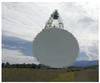 |
Fig. 1 The Green Bank Telescope in a view that shows its unblocked 100-m diameter aperture. |
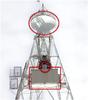 |
Fig. 2 The focal area of the GBT as seen from the surface of the main reflector, showing outlined in red, bottom to top, (i) the receiver room; with (ii) the L-band feed horn pointing upward at (iii) the 8-m subreflector. Just below the lower edge of the subreflector the lower portion of a screen is visible. This functions to direct feed spillover radiation that would otherwise strike the telescope arm back into the main reflector and onto the sky. |
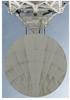 |
Fig. 3 The GBT subreflector and feed arm seen from the secondary focal point atop the receiver room. The screen redirects feed spillover away from the arm and down into the main reflector. |
The 21-cm “L-band” receiver used for these measurements is located at the secondary Gregorian focus and illuminates an 8-m diameter subreflector with an average edge taper of −14.7 dB (Srikanth 1993). The receiver is cryogenically cooled, accepts dual linear polarization, and has a total system temperature, Tsys, at the zenith of 18 K. A diode injects a fixed amount of noise into the waveguide just after the feed horn, before the polarizer and amplifier, and can be modulated rapidly for calibration. This was used to establish a preliminary scale for the antenna temperature, Ta. These noise sources are typically very stable; we see no evidence for variation of the L-band receiver calibration diode over several years (Sect. 7).
3. H I 21-cm line data acquisition
3.1. Mapping
The H i 21-cm observations discussed here were made with on-the-fly mapping: “scanning” or moving the telescope in one direction, typically Galactic longitude or right ascension, while taking data continuously. The integration time and telescope scan rate must be chosen so that samples are taken no more coarsely than at the Nyquist interval, ≈ FWHM/2.4 = 3.8′ for the GBT at 21 cm, and ideally at half that interval to avoid beam broadening in the scanning direction (Mangum et al. 2007). Areas were mapped by stepping the scans in the fixed coordinate (the cross-scan direction) and reversing the scan direction. In the H i surveys discussed here (Martin et al., in prep.) scans up to 5° long were made, but for practical purposes larger regions were broken up into smaller areas with dimensions between 2° × 2° and 4° × 4° that were mapped independently.
3.2. Spectrometer setup
The GBT autocorrelation spectrometer as configured for these measurements has 16k channels over a 12.5 MHz band with nine-level sampling in each linear polarization, for a velocity resolution of 0.16 km s-1 in the 21-cm line. Early in the data reduction procedure the resolution was reduced to 0.80 km s-1 by filtering the spectra with an eleven-channel Hanning smoothing function and resampling every fifth channel. This maintains the independence of each channel, while minimizing aliasing effects.
The local oscillator was modulated to move the center of the spectrometer band between a “signal” and “reference” frequency, separated by 2.5 MHz (528 km s-1). The noise source was modulated synchronously with the frequency switching to calibrate the receiver gain at both signal and reference frequencies every second. Because the modulated separation is much smaller than the 12.5 MHz covered instantaneously by the spectrometer, the emission in the 21-cm line was always being observed. This “in-band” frequency switching gives a factor of two increase in observing speed over “out-of-band” frequency switching, and an rms noise in antenna temperature, σTa, of approximately 0.25 K in a 1 km s-1 channel in 1 second for the average of the two polarizations. For the basic integration time for the survey data, 4 s, and velocity resolution 0.80 km s-1, the resulting rms noise is 0.16 K for emission-free channels (see Sect. 7.1). Some regions were measured several times to check the reproducibility and to improve the sensitivity.
3.3. Spectral baselines
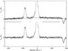 |
Fig. 4 Brightness temperature spectrum from the North Ecliptic Pole (NEP) data cube at
|

The frequency-switched spectra produced by the GBT spectrometer (e.g., Fig. 4) have remarkably flat instrumental baselines over the central 4 MHz, even more so for the XX compared to the YY polarization. Nevertheless, an important step in our GBT data reduction procedure (Sect. 4) is removal of any residual instrumental baseline. As is usual, the baseline is approximated by a low-order polynomial whose coefficients are fit by linear least-squares to the “emission-free” channels of each spectrum. For the GBT spectra we found that over the central ~4 MHz (−450 < v < +400 km s-1) a third-order polynomial was adequate, the next order term being not statistically justified. Except for diagnostic purposes, we fit baselines to spectra after correction for stray radiation and assembly into a data cube (Sect. 4.2). In a very few spectra, out-of-band interference results in unsalvageable spectra with high-order polynomial baselines. These are easily identified by eye, and in most cases we were able to reobserve these positions. Alternatively, these spectra are flagged for exclusion from the map-making process.
For our mapping observations with the GBT, the instrumental baseline was found to change slowly with time, so that the coefficients of the polynomial fit are highly correlated between spectra along a scan. For noisy spectra there are potential advantages to fitting a baseline to the average of sequential spectra (Lockman et al. 1986), but we did not implement this as fitting of individual polynomials gave adequate results. It is possible to take advantage of an iterative baseline fitting technique. This brings in more channels than one normally obtains from a conservative estimate of the location of the emission-free end channels for a particular map, even locating emission-free parts of the spectrum between emission features.
We fit baselines following the iterative technique used by Hartmann (1994) for the Leiden/Dwingeloo Survey. Prior to any fitting, each spectrum is smoothed by a 20-channel (roughly 16 km s-1) boxcar to accentuate real velocity features. We used Hartmann’s definition of a “velocity feature” present in a residual spectrum from which an estimated baseline has been removed. These are found by first identifying a significant (4.0σ) positive peak and then adding neighbouring channels until the residual goes negative; ten additional channels (about 8 km s-1) at both ends of each velocity feature are also flagged for omission. Following the identification of all such features, there remain the “emission-free” baseline channels to be used in the next fit. The smoothed baseline spectrum is fit successively with a series of polynomials monotonically increasing from linear to third-order, after every iteration subtracting this updated baseline and identifying and flagging new velocity features with significant residual peaks. Because the spectra are frequency-switched, any velocity emission feature will show up as a half-amplitude inverted feature offset by the switching frequency, 2.5 MHz. These channels are also flagged for exclusion. Finally, a third-order polynomial is fit to the remaining list of emission-free channels in the original spectrum and subtracted. Usually ~600 emission-free channels are used for the fit. Figure 4 illustrates a typical result of the iterative baseline fitting process, for a typical instrumental baseline.
Occasionally we found H i emission from background galaxies in our spectra, usually in the end channels beyond the Galactic emission, but sometimes even overlapping it. This makes determining the instrumental baseline challenging. While this can be treated on a case-by-case basis, these pixels are simply masked as unsuitable for analysis of Galactic H i.
3.4. Treatment of radio frequency interference (RFI)
The main source of RFI in these data is an oscillator in the GBT receiver room which can produce narrow-band spurious signals in the data. These are extremely stable and ≪ 1 kHz in width. They can be identified easily and removed. A series of eight frequency ranges in which RFI had been seen were systematically inspected by averaging many spectra together in the topocentric velocity frame of reference. Any 3.5σ positive deviations from the median over the suspect frequency range were flagged. Finally data in a group of five channels around the flagged frequency were replaced with values from a linear interpolation of the surrounding channels. This channel replacement is done at the highest velocity resolution (0.16 km s-1) on the four observed spectrometer phases (sig/calon, sig/caloff, ref/calon, ref/caloff) prior to producing the final calibrated frequency-switched spectra and prior to any subsequent spectral smoothing. Efforts are underway to replace the interfering device.
4. Data reduction
The measured quantity, Ta, is related to the
21-cm H i sky brightness Tb by 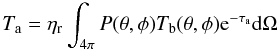 (1)where
e−τa is the direction-dependent atmospheric
extinction and P is the antenna power pattern; the integration is over the
entire 4π sr and this “all-sky” integral of P is unity
(later we also refer to the antenna gain G = 4πP relative
to isotropic, where by definition
Gisotropic(θ,φ) = 1). The quantity
ηr accounts for resistive losses in the system which are less
than 1%. Our procedure in Sect. 5.2 for calibration
of Ta produces an antenna temperature scale that is
independent of ηr and we will thus drop this factor from
subsequent equations. Equation (1) can be
separated into terms that come from the main beam and from elsewhere on the sky:
(1)where
e−τa is the direction-dependent atmospheric
extinction and P is the antenna power pattern; the integration is over the
entire 4π sr and this “all-sky” integral of P is unity
(later we also refer to the antenna gain G = 4πP relative
to isotropic, where by definition
Gisotropic(θ,φ) = 1). The quantity
ηr accounts for resistive losses in the system which are less
than 1%. Our procedure in Sect. 5.2 for calibration
of Ta produces an antenna temperature scale that is
independent of ηr and we will thus drop this factor from
subsequent equations. Equation (1) can be
separated into terms that come from the main beam and from elsewhere on the sky:
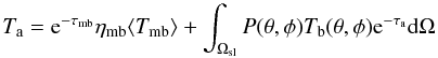 (2)where
e−τmb is the atmospheric extinction in the
direction of the main beam, ηmb, the main beam efficiency, is
the fraction of the total power accounted for by the main beam over Ωmb,
Ωsl is the area of the sky outside the main beam
(Ωsl = 4π−Ωmb). The desired quantity to be
measured, ⟨ Tmb ⟩ , is the H i brightness temperature
averaged over the main beam:
(2)where
e−τmb is the atmospheric extinction in the
direction of the main beam, ηmb, the main beam efficiency, is
the fraction of the total power accounted for by the main beam over Ωmb,
Ωsl is the area of the sky outside the main beam
(Ωsl = 4π−Ωmb). The desired quantity to be
measured, ⟨ Tmb ⟩ , is the H i brightness temperature
averaged over the main beam: 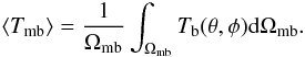 (3)While
Tb and Ta are functions of
frequency because of Doppler shift, it is assumed that the other quantities are constant
over the relatively narrow frequency range of Galactic HI emission. Equation (2) can thus be written
(3)While
Tb and Ta are functions of
frequency because of Doppler shift, it is assumed that the other quantities are constant
over the relatively narrow frequency range of Galactic HI emission. Equation (2) can thus be written ![Mathematical equation: \begin{equation} \langle T_{\mathrm{mb}} \rangle = {\mathrm{e}^{\tau_{\mathrm{mb}}}\over{\eta_{\mathrm{mb}}}} \left[ T_{\mathrm{a}} - \int_{\Omega_{\mathrm{sl}}} P(\theta,\phi) T_{\mathrm{b}}(\theta,\phi)\mathrm{e}^{-\tau_{\mathrm a}} \mathrm{d}\Omega \right]. \label{removestray} \end{equation}](/articles/aa/full_html/2011/12/aa17656-11/aa17656-11-eq55.png) (4)The aperture efficiency
ηa and beam efficiency ηmb are not
necessarily independent (e.g., Goldsmith 2002). For a
dish of diameter, D, at wavelength, λ, with a Gaussian
main beam, θFWHM, and with typical values for
the main reflector edge taper, we have
ηmb ≡ Ωmb/Ωa,
Ωa = 4λ2/(ηaπD2),
(4)The aperture efficiency
ηa and beam efficiency ηmb are not
necessarily independent (e.g., Goldsmith 2002). For a
dish of diameter, D, at wavelength, λ, with a Gaussian
main beam, θFWHM, and with typical values for
the main reflector edge taper, we have
ηmb ≡ Ωmb/Ωa,
Ωa = 4λ2/(ηaπD2),
 , and
θFWHM ≈ 1.25λ/D.
Thus, ηmb ≈ 1.4ηa for the GBT at
21 cm. However, this relationship is not necessarily precise for real systems, and so we
treat the two terms as independent quantities that have to be derived and checked
separately.
, and
θFWHM ≈ 1.25λ/D.
Thus, ηmb ≈ 1.4ηa for the GBT at
21 cm. However, this relationship is not necessarily precise for real systems, and so we
treat the two terms as independent quantities that have to be derived and checked
separately.
For simplicity, the observable ⟨ Tmb ⟩ will be referred to as Tmb or simply T from henceforth.
4.1. Stray radiation
The second term in Eq. (4) accounts for
H i emission that enters the receiver through the sidelobes of the telescope
rather than through the main beam. This is called “stray” radiation. Just as the main beam
efficiency, ηmb, reflects the fraction of the power pattern in
the main beam, we define a sidelobe efficiency, ηsl,
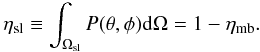 (5)The unblocked
aperture of the GBT eliminates the scattering sidelobes that plague most other radio
telescopes, but at 21 cm the relatively low edge taper of the feed (originating from
mechanical limitations on its size and weight, see Norrod
& Srikanth 1996) results in a “spillover lobe” past the secondary
reflector. Because there is 21-cm H i emission from all directions of the sky at
a level NHI ≳ 4 × 1019 cm-2 (Lockman et al. 1986; Jahoda et al. 1990), there will be a contribution to every spectrum from
H i emission entering through the sidelobes, and so the “stray” radiation
spectrum must be calculated and removed as a part of data reduction and calibration. Prior
to construction of the GBT the only unblocked radio telescope useful for 21-cm
measurements was the Bell Labs horn-reflector which had a main beam size ≈ 3° × 2° and a
spillover lobe as well (Wrixon & Heiles
1972; Kuntz & Danly 1992)
(5)The unblocked
aperture of the GBT eliminates the scattering sidelobes that plague most other radio
telescopes, but at 21 cm the relatively low edge taper of the feed (originating from
mechanical limitations on its size and weight, see Norrod
& Srikanth 1996) results in a “spillover lobe” past the secondary
reflector. Because there is 21-cm H i emission from all directions of the sky at
a level NHI ≳ 4 × 1019 cm-2 (Lockman et al. 1986; Jahoda et al. 1990), there will be a contribution to every spectrum from
H i emission entering through the sidelobes, and so the “stray” radiation
spectrum must be calculated and removed as a part of data reduction and calibration. Prior
to construction of the GBT the only unblocked radio telescope useful for 21-cm
measurements was the Bell Labs horn-reflector which had a main beam size ≈ 3° × 2° and a
spillover lobe as well (Wrixon & Heiles
1972; Kuntz & Danly 1992)
Stray radiation originating from large angles is Doppler-shifted with respect to the direction of the main beam, so that the stray radiation spectrum correctly shifted to the local standard of rest (LSR) depends not only on the location of the sidelobe on the sky but also on the date and time of the observation (Kalberla et al. 2005). For an Alt-Az telescope like the GBT, the sidelobe pattern, which is fixed in telescope coordinates, also rotates on the sky about the main beam as the Local Sidereal Time (LST) changes. A direction observed at varying LST will have a varying component of stray radiation.
Stray radiation has been an issue for Galactic 21-cm science for 50 years (van Woerden et al. 1962; Heiles & Wrixon 1976) and many groups have devised methods to suppress or remove it (e.g., Wrixon & Heiles 1972; Kalberla et al. 1980; Lockman et al. 1986; Hartmann et al. 1996; Higgs et al. 2005; Kalberla et al. 2010). The most accurate methods solve Eq. (4) for ⟨ Tmb ⟩ using models of the antenna power pattern, P, and all-sky Tb(θ,φ) maps.
Because the most important sidelobes of the GBT cover large areas of the sky, relatively low angular resolution 21-cm surveys can be used for the Tb(θ,φ) term in estimating the stray component, e.g., the Leiden/Argentine/Bonn (LAB) survey (Kalberla et al. 2005). However, this is not true for the first few diffraction sidelobes that lie close to the main beam. These have angular structure on scales like that of the main beam and would require knowledge of the H i sky at that level of detail for their removal. For the GBT, however, the near sidelobes are quite small and contain <1% of the telescope response (Sect. 5.1). We do not correct for these, in effect assuming that their small component of the telescope’s response samples nearly the same emission as the main beam.
4.2. Procedure
The data reduction procedure thus involves calibration of the intensity scale to antenna temperature, calculation and subtraction of the stray radiation spectrum, and correction for the main beam efficiency and the atmosphere. Data reduction additionally requires removal of an instrumental baseline, and for maps, interpolation of the sampled spectra into a data cube. The latter two steps are sometimes interchanged; the interpolated spectra, especially if combining several observations of a region, are less noisy so that baseline removal at that final stage might be preferable.
The initial calibration of the data to an approximate Ta antenna temperature scale used values for the receiver calibration noise source that were determined by measurements in the laboratory for each receiver polarization channel. This part of the data reduction was performed using the NRAO program GBTIDL. A constant calibration temperature was assumed over the 12.5-MHz band. We checked this part of the calibration, and we correct it by a small amount using our own measurements and calculations as described below in Sect. 5.2.
Our implementation of the stray radiation correction is described in Sect. 6.4 and Appendix C, making use of the sidelobe pattern established in Sect. 6.1.
Calculation of the main beam efficiency is described in Sect. 5.1. The NRAO data reduction program GBTIDL will perform an approximate correction for atmospheric extinction1 but we chose to make the correction independently, using τzenith = 0.01036 ± 0.00059, the weighted mean of the measured values of Williams (1973) and van Zee et al. (1997), with a model for the atmospheric air mass (Appendix C).
After the spectra were calibrated and corrected for stray radiation, an instrumental baseline was removed from each spectrum by fitting a third-order polynomial to emission-free velocities. It is important that the stray radiation be removed before baseline fitting, lest weak stray wings be mistaken for instrumental baseline. For mapped regions, data cubes were constructed in classic AIPS, averaging together spectra from the two polarizations, using the optimal tapered Bessel function for interpolation (Mangum et al. 2007). In our data reduction procedure, baselines were removed after creating the cubes. For details see Sect. 3.3.
Note that nowhere during this procedure are “standard” H i regions, like S6 (Williams 1973) and S8 (Kalberla et al. 1982), used to calibrate the GBT intensity scale. Because of the clean optics of the GBT, we preferred to determine its characteristics from basic calculations and radio continuum flux density calibration sources. We did, however, observe the above two standard H i directions and we discuss these measurements in Sects. 7.4 and 8.1. We also compared our spectra to those of the LAB survey (Sect. 8.2).
5. Aperture and main beam efficiencies
5.1. Calculation of the efficiencies
A theoretical estimate of the all-sky response of the GBT was calculated using a
reflector antenna code developed at the Ohio State University as described in
Appendix A. This incorporates information on the
detailed illumination pattern of the 21-cm feed on the GBT subreflector as measured after
construction of the receiver (Srikanth 1993).
Table 1 shows the calculated on-axis or forward
gain and aperture efficiency as a function of frequency for the L-band
receiver. The variation in ηa results from measured changes in
the L-band receiver illumination pattern with frequency. The calculated
gain G(θ,φ) of the GBT at 1.4 GHz within
 of the main beam is shown in
Fig. 5 for radial cuts along polar angle
θ in planes at several angles φ (see the angle
definitions in Appendix A). The units are dBi
(logarithmic units relative to an isotropic beam) and the value at
θ = 0° is that in Table 1. The first sidelobe is calculated to be 29 dB below the forward peak of the
main beam. Observations also indicate that the GBT’s main beam is exceptionally clean with
near-in sidelobes all about 30 dB below the main beam gain (Robishaw & Heiles 2009).
of the main beam is shown in
Fig. 5 for radial cuts along polar angle
θ in planes at several angles φ (see the angle
definitions in Appendix A). The units are dBi
(logarithmic units relative to an isotropic beam) and the value at
θ = 0° is that in Table 1. The first sidelobe is calculated to be 29 dB below the forward peak of the
main beam. Observations also indicate that the GBT’s main beam is exceptionally clean with
near-in sidelobes all about 30 dB below the main beam gain (Robishaw & Heiles 2009).
Table 2 gives the fraction of the total power
pattern lying within a given radius around the main beam, at radii corresponding to the
minima in Fig. 5. This shows that 87.7% of the
antenna response lies within  of the main beam, increasing by
only a small amount to 88.1% at radius, consistent with the
observations that the near sidelobes are at very low levels. We adopt a value
ηmb = 0.88. This value was also derived independently during
the initial calibration of the L-band receiver on the GBT (Heiles et al. 2003).
of the main beam, increasing by
only a small amount to 88.1% at radius, consistent with the
observations that the near sidelobes are at very low levels. We adopt a value
ηmb = 0.88. This value was also derived independently during
the initial calibration of the L-band receiver on the GBT (Heiles et al. 2003).
We define the “far” sidelobes as those arising at angles
θ > 1° from the main beam. Compared to
ηsl ≈ 0.1, the potential for stray radiation arising within
 of the
main beam is negligible (Δη ≈ 0.004); furthermore, the brightness of this
radiation Tb will not be grossly different from that seen on
axis, and it will not be Doppler shifted as in the far sidelobes.
of the
main beam is negligible (Δη ≈ 0.004); furthermore, the brightness of this
radiation Tb will not be grossly different from that seen on
axis, and it will not be Doppler shifted as in the far sidelobes.
Calculated forward gain and aperture efficiency for the GBT L-band receiver.
Calculated fractional power pattern at 1.4 GHz as a function of angle from the beam center.
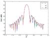 |
Fig. 5 GBT antenna gain above isotropic for the main beam and near sidelobes at 1.4 GHz, as a function of polar angle θ from the main beam in several planes defined by φ (see Appendix A for the antenna code used for this calculation). The forward gain is 61.6 dBi (Table 1). |
5.2. Establishing the antenna temperature scale
The preliminary antenna temperature calibration assumes that the noise source has no frequency dependence over the range of our observations. To check this we observed the standard radio continuum source 3C 286 in spectral line mode and measured the precise value of the receiver noise source averaged in 50 km s-1 intervals around the Galactic 21-cm line. When the two linearly polarized channels are averaged the noise source varies little with frequency, with a peak-to-peak fluctuation about the mean of only 1.2% over 600 km s-1 around the 21-cm line. Thus the assumption of a constant calibration noise across our band will not contribute a significant uncertainty to the H i measurements when both polarizations are combined.
The absolute value of the noise source was checked using the flux density standard 3C 286 (Ott et al. 1994) and the aperture efficiency derived from the electromagnetic calculations (Sect. 5.1). From 13 measurements at two epochs we derive a calibration temperature of 1.495 ± 0.013 K (1σ), a value that is in the ratio 1.024 ± 0.009 to that measured in the laboratory. As 3C 286 has significant linear polarized emission this is for the average of the two polarizations. A smaller number of measurements on 3C 295 gives a result that is identical to within the uncertainties. We thus increased the preliminary antenna temperatures by this ratio to place spectra on an accurate Ta scale. Note that this calibration, derived from an external radio source, subsumes within it any correction necessary for ohmic losses in the entire system.
5.3. A check using the Moon
The Ta scale and value of ηmb were further checked by continuum observations of the Moon, assumed to have a constant brightness temperature of 225 ± 5 K at 1.4 GHz (Keihm & Langseth 1975) and taking into account that only a part of the response pattern shown in Fig. 5 lies within the disk of the Moon. Measurements at several epochs give a measured to expected ratio 0.97 ± 0.025 (1σ), where the uncertainty includes the scatter in the measurements and in the assumed Tb of the Moon. Because we measure the Moon relative to the nearby sky, these observations are not susceptible to radiation in the far sidelobes and so are an uncomplicated test of both the Ta scale and ηmb determination. We conclude that our calibration does not have systematic errors that exceed a few percent.
6. GBT all-sky response
Calculating the stray 21-cm component requires knowledge of the antenna response in all directions on the sky. Important sidelobes can occur at a level 50 dB below that of the main beam, and thus be quite difficult to measure. Nonetheless, they can contain several percent of the telescope’s total response because they cover a large area on the sky. In an analysis of the 21-cm beam pattern of the Effelsberg 100-m antenna, Kalberla et al. (1980) found 70% of the response within 15′ of the main beam, another 12% in the range 15′ < θ < 4°, and the remaining 18% at 4° < θ < 180°. An unblocked antenna like the GBT has much lower sidelobe levels, but at 21 cm there is still an important contribution to stray radiation due to spillover past the subreflector. Note that the sidelobe pattern for the GBT is not symmetrical about the main beam, but for comparison more than 87% of the response is within 15′ of the main beam (Table 2), with another 1.8% in the range 15′ < θ < 4°.
To determine the all-sky response P of the GBT we first used the reflector antenna code (Sect. 5.1) to find the calculated response. The results were used to set the aperture efficiency, main beam efficiency, and the power pattern within θ < 1° of the main beam.
These calculations also give a general picture of the location and amplitude of the far sidelobes. Key features of the sidelobes can also be understood using simple near-field diffraction theory as discussed in Appendix B. Because the antenna code uses only an approximation to the complex structure of the GBT, a more accurate determination was accomplished by measuring the sidelobes directly over much of the region within 60° of the main beam, exploiting the Sun as a strong radio continuum source. The Sun can be treated as a point source relative to the angular size of most of the structure in the sidelobes.
6.1. Sidelobe measurements using the Sun
6.1.1. Observations
The observations were made on three different occasions, during times of the year when confusion with radio emission from the Galactic plane would be minimized. Data were taken over a 20 MHz band centered on 1420 MHz. The mapping procedure consisted of raster scans, moving the telescope either in elevation (“vertical” scans) or azimuth (“horizontal” scans). Figure 6 shows the position of the Sun relative to the main beam during the scans used to determine the sidelobes, in terms of the vertical separation in elevation V from the beam center, and the horizontal separation in the perpendicular (cross-elevation) direction H. If the beam is pointed at the horizon at an azimuth of 0°, then V corresponds to elevation and H to azimuth. We define H = θcosφ and V = −θsinφ, where θ is the angular distance from the beam center and φ is the azimuthal angle around the beam, with φ = 0° orthogonal to the antenna symmetry plane and φ = 90° corresponding to the downward direction in elevation (away from the GBT arm; see Fig. 1 and Appendix A).
The sunscans cover the most of the region −20° < V < +55° and −17° < H < +55°. The left-right reflection symmetry of the telescope implies that a sunscan at –H should be identical to one at H. The data were recorded at intervals of between 2 and 10 s, corresponding to separations of a few arcminutes on the sky at the adopted scan rates.
The initial data set consisted of “vertical” raster scans spaced 2°−4° apart. Among these, the “distant vertical” scans lying beyond H ~ 35° from the main beam (dotted lines at right in Fig. 6) showed no evidence of sidelobes above the noise level. The theoretical values for these scans are small enough to be consistent with a measured value of zero, considering the uncertainties in the data.
The second data set consisted of “horizontal” scans spaced by about 1° in V. The third set consisted of “vertical” scans, most spaced by about 1° in H, but including a group with 30′ spacing refining the coverage of the range |H| < 3°. Although we were not able to measure the power pattern to large negative angles H, both the theoretical calculations and our observations indicate that the pattern is symmetric about a vertical line (H = 0°) through the center of the main beam.
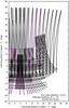 |
Fig. 6 Mapping the GBT sidelobe pattern using the Sun. Heavy lines indicate the position of the Sun relative to the main beam during the scan. Thin magenta lines indicate scans reflected in the beam’s line of symmetry (i.e., with the H coordinate replaced by −H). Dotted lines at high H show measurements that were not used because they showed no visible sidelobes above the noise. The center of the subreflector is 12.3° above the main beam. |
6.1.2. Data reduction and relative calibration of the observations of the Sun
A baseline was set using the longest scans, assuming that the sidelobes many tens of degrees from the main beam are relatively negligible; the calculations suggest that away from the spillover lobe the typical sidelobe has an amplitude of −75 dB with respect to the main beam. Backgrounds had to be subtracted, consisting of a large constant component plus a smaller elevation-dependent component with a slight amount of curvature which was well fitted by an exponential which accounts for atmospheric emission variations with elevation. The most distant vertical scans that showed no strong sidelobes were used to examine the elevation dependence of the background signal in the recorded data. Both background components varied to some extent from scan to scan, with the constant component also being slightly different for the two polarizations. Spikes in the data due to RFI were also removed. The numerous scan crossings were used to fix the amplitude of the shorter scans. Consistency of these scan crossings, and of the scans symmetric about H = 0°, indicated an accuracy of approximately 10% in the background-subtracted scans; the horizontal scans appeared somewhat less accurate, possibly due to the variation in the height of the horizon along a horizontal scan.
At 1.4 GHz the Sun can have significant temporal variations in its emission. Relative normalizations of the three datasets were determined from the numerous scan crossing points. We could not find 21 cm measurements of the solar flux for the periods of our observations, and so we used the solar flux monitor measurements at 10.6 cm from the DRAO2 to check that the relative normalization factors were consistent with the ratios of the solar flux. The second and third datasets were obtained near the solar activity minimum, and required only a small relative normalization factor; the first dataset had been obtained at at time when the solar emission was approximately twice as large, requiring a relative normalization factor of about two.
Scans were smoothed along the scan direction, and linear interpolation was used to estimate values between the scans in a direction approximately perpendicular to the scan direction. Observations at negative azimuth angles were “flipped” to positive azimuth, providing additional coverage and consistency checks. Where scans crossed or approached closer than 30′ to each other, a weighted average was used at their positions to avoid any sudden jumps. Separate interpolations were made for each of the three datasets, with a weighting approximately proportional to the density of the observations on the sky.
The result is a map of the relative GBT beam pattern covering the important sidelobes within the range |H| < 32° (horizontal extent) and −20° < V < +55° (vertical extent).
6.1.3. Determining the amplitude scale of the measured sidelobes
The power pattern measured using the Sun needs to be scaled by an amount determined below, because the absolute brightness of the Sun at the times of observation is not known to the required precision. Because the sidelobes are fixed with respect to the GBT, as a given direction is observed the sidelobes will cross regions of different 21-cm Tb causing the stray radiation component to vary throughout the day. There are also different Doppler shifts. We took advantage of these temporal changes to estimate the scaling of the measured sidelobes by mapping a large area around the north ecliptic pole (NEP) containing >4 × 10⁴ unique positions. H i spectra were measured at each position on three separate occasions at different ranges in azimuth and elevation. For each position the spectra were reduced, calibrated, and corrected for stray radiation using Eq. (4) with a range of scalings which, when added to the calculated part of the sidelobe pattern, gave a range of values of ηsl. The amount of the telescope response in the calculated portion of the far sidelobes, which is generally the region at θ ≳ 60°, is 0.0187.
A histogram of the differences between each of the three observations of the integral over the H i line profile (W, in K km s-1) and their mean is shown in Fig. 7 for different representative ηsl. The black dotted curve shows the large scatter in the measurements when there is no correction for stray radiation. The stray radiation correction is quite effective: the dispersion decreases to a minimum as the scaling increases, then subsequently increases. The optimum scaling of the empirical sidelobe pattern is the one that minimizes the dispersion, near ηsl = 0.097.
A similar analysis, looking directly at differences in Tmb channel by channel instead of differences in the area W, was performed on the NEP field and on other areas that were observed multiple times during the course of the Martin et al. (in prep.) surveys. For the spectra in the NEP field, this analysis yields a value of ηsl = 0.1014 ± 0.0018, where the uncertainty is solely a measure of the statistical accuracy of ηsl; it does not take into account the accuracy of the sidelobe pattern. This places the above NEP W result within 2σ, indicating the consistency of the two analyses. For all additional (non-NEP) spectra – most of which only have two repeat visits – the Tmb analysis yields a value of ηsl = 0.0947 ± 0.0032. The statistical error was obtained by a chi-squared analysis; to determine the number of degrees of freedom, it was assumed that each continuously-observed “chunk” of sky (i.e., wherein all spectra have similar sky positions and LST values) could be considered an independent measurement of ηsl. There are proportionally a larger number of spectra in the NEP field, but they are all representative of a single patch of the sky with three repeated observations, and statistically will have more similar LST values – observations of nearly the same patch of sky at nearly the same LST do not yield entirely independent measurements of ηsl. Obtaining the best ηsl separately for all nine subregions observed in the NEP survey yields values that are all within 0.5σ of the best overall NEP value, according to their individual statistical errors, unlike the 13 separate non-NEP regions, where the scatter is consistent with the statistical errors. Thus the formal statistical error from the NEP measurement underestimates its true error, which is probably closer to the non-NEP error estimate, and so we decided that an average of the two values (NEP and non-NEP) would yield a less biased result for ηsl. Consequently, we have adopted ηsl = 0.0981 ± 0.0023 to set the amplitude of the measured sidelobes on a correct scale relative to the GBT main beam.
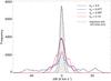 |
Fig. 7 Estimating the optimal value of ηsl using three repeated observations at more than 4 × 10⁴ positions near the NEP, each repeat having different stray radiation. For different assumed ηsl, the difference between each observation of W and the mean of the three was calculated for every position. Histograms of the resulting distributions of differences show the sensitivity to ηsl, including the dotted curve for no stray radiation correction. Correction is clearly beneficial, and a minimum dispersion occurs for ηsl ≈ 0.097. Note that the dispersion does not quite reach the minimum predicted from line noise and baseline uncertainties alone (dashed line, see Sect. 7.2). |
Note that ηmb + ηsl ≈ 0.98; we cannot account for about 2% of the power. Cases were tested where an isotropic component ηiso was added to the sidelobes to bring the total beam power closer to unity. However, even ηiso = 0.01 (i.e., an increase of 0.005 in the sidelobe power seen by the sky) yielded significantly more overcorrection, with parts of stray-corrected spectra going negative. The formal uncertainty of 0.0023 refers to overall increases or decreases in the measured sidelobe. Modifications to the shape of the measured sidelobes (e.g., an isotropic component; see also Appendix B.6), would yield a different “best ηsl” value. Considering possible variations yields a somewhat larger error estimate of 0.005.
6.2. Combining the calculated and measured power pattern
The adopted power pattern P is a combination of the calculations of
Sect. 5.1 with the measurements of the Sun of
Sect. 6.1. Measured values at
 begin to differ from the
calculated values, while at
begin to differ from the
calculated values, while at  the coarse, half-degree spacing
of the measurements is insufficient to probe the smaller-scale beam structure there; for
both these regions, differences between measurement and calculation can exceed a factor
of 2. However, for θ ≈ 1°, measured values (P convolved
with the Sun) typically agree to better than 20% with smoothed calculated values
(P convolved with a paraboloid to yield a resolution of
0
the coarse, half-degree spacing
of the measurements is insufficient to probe the smaller-scale beam structure there; for
both these regions, differences between measurement and calculation can exceed a factor
of 2. However, for θ ≈ 1°, measured values (P convolved
with the Sun) typically agree to better than 20% with smoothed calculated values
(P convolved with a paraboloid to yield a resolution of
0 5) – this is
nearly the best that can be expected from the inherent uncertainties in the measurements.
Therefore, for
5) – this is
nearly the best that can be expected from the inherent uncertainties in the measurements.
Therefore, for  , we make a smooth
switchover from the (convolved) calculated P to the measured one. As we
correct for sidelobes only at θ ≳ 1°, this switchover has a negligible
effect on the results.
, we make a smooth
switchover from the (convolved) calculated P to the measured one. As we
correct for sidelobes only at θ ≳ 1°, this switchover has a negligible
effect on the results.
The theoretical values for P outside the region measured using the Sun
are small enough to be consistent with a measured value of zero, considering the
uncertainties in the data. Some of the back sidelobes are simply not accessible, being
below the horizon; they are also not used in our evaluation of the stray radiation
(Sect. 6.4). Therefore at angles beyond where we
were able to probe directly, the theoretical calculations of P were again
adopted with a smooth switchover at the outer 05 edge of the
measured region to prevent any possible discontinuities in the adopted P.
6.3. Properties of the adopted response pattern
Figure 8 is a contour map of the inner part of the derived GBT power pattern probed with the Sun; this is G in dBi. The obvious symmetry about a vertical line through the center of the main beam (H = 0°) is by construction, as discussed above in Sect. 6.1.1. Other displays of the GBT sidelobe pattern are given in Figs. 9 and 10; these are on a linear scale and are for P = 4πG.
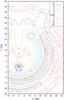 |
Fig. 8 Contours of the measured GBT far sidelobe gain G, relative to isotropic. The main beam is at the origin (indicated by the solid dot), and would peak at + 61.6 dBi. The H and V coordinates are the same as in Fig. 6. Elevation increases upward in the plot and the direction to the center of the subreflector is at V = 12.3°. The main “spillover lobe” is outlined by the yellow 0 dBi contour, with the blue 4 dBi and magenta 5 dBi contours defining its ridge; curving as a ring from below the main beam at (H,V) ~ (0°, −7°), it extends to about (H,V) ~ (12°,28°), beyond which it is blocked by the screen on the telescope arm (note that this blockage also yields a ridge stretching upward from the subreflector center along the edge of the gap at an angle about 35° from the vertical; this ridge passes through the end of the spillover lobe). Complementary to this missing part of the spillover lobe caused by the screen are the twin peaks below the main beam, at (H,V) ~ (± 1°, −3°), visible in the heavy black 10 dBi and thin gray 15 dBi contours. Outside the spillover lobe are three lower-amplitude rings (at radii θ ~ 26°, 29.5°, and 33° from the subreflector center). Inside is the Arago spot and surrounding rings centred at 11.879° on the axis above the main beam. Some features are easier to see in the 3Dplots of Figs. 9 and 10. Outside the faint spillover rings and outside the region (| H| < 35°,20° < V < 53°), the sidelobe levels are taken from the antenna code calculations. |
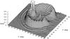 |
Fig. 9 GBT response pattern P, as measured from scans of the Sun, on a linear scale. The H and V coordinates are the same as in Figs. 6 and 8. Note that this plot has been rotated so that its features are more easily visible – the vertical coordinate V increases from left to right in this figure. The truncated peak at center-left in this figure comprises both the main beam at (H,V) = (0,0) and the double-peak feature at (H,V) ~ (± 1°, −3°); the peak of the main beam would be far offscale at P = 1.12 × 10⁵. Near the center of the spillover lobe, the Arago spot is visible. The gap at high V in the spillover lobe and its surrounding rings arises from the presence of the reflecting screen at the subreflector edge. |
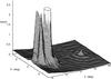 |
Fig. 10 Measured GBT response pattern P, as in Fig. 9, but for sidelobes closer to the main beam. The Arago spot, peaking at ≈ 0.25, is visible at the right, along with its surrounding rings. The double-peak feature at (H,V) ~ (±1°, −3°) appears just to the left of the (truncated) main beam, with height P ≈ 2.6. This contains the power scattered from the forward spillover lobe by the reflecting screen on the feed arm (Fig. 3). The peak of the main beam would be far offscale at P = 1.12 × 10⁵. |
Away from the main beam, the power pattern is dominated by the forward spillover sidelobe, the arc of radiation from the secondary feed spilled past the subreflector (see Fig. 9). In symmetric antennas such spillover sidelobes are symmetrical about the main beam, but with the offset subreflector of the GBT (Norrod & Srikanth 1996) it is centered roughly on the cone axis defining the secondary, displaced by about V = 12° above the main beam in elevation (it retains left-right symmetry but is not circularly symmetric). This spillover lobe results from near-field (Fresnel) diffraction of the feed illumination from the sharp edge of the subreflector, which can be thought of as a disk occulting the sky. Our measurements of the diameters of the main spillover lobe and the fainter rings outside it are consistent with this, given the GBT geometry (Appendix B). The peak level along the ridge of this main spillover lobe is quite low, about +5 dB above isotropic and therefore about 57 dB below the main beam, but because of the large area it contributes substantially to ηsl and the stray radiation.
The gap in the spillover lobe at (H,V) ~ (0°,30°) is caused by the arm that supports the GBT subreflector, specifically a reflecting screen attached to that arm (Fig. 3). It deflects the spillover radiation back into the main dish over a 40° segment of the spillover lobe. The reflected radiation emerges on the sky as a pair of sidelobes well away from the main beam on the opposite side, at about H = ± 1°,V = −3° (Fig. 8). Each peak is elongated by about 1°, approximately along the azimuthal direction as seen at the left in Fig. 10. They have a peak amplitude about ten times that of the spillover lobe, but comprise only a small part of the total beam integral, comparable to the portion of the major ring removed in the wedge, qualitatively consistent with conservation of energy. This is discussed in more detail in Sect. B.4.
A more minor, but interesting, feature in the GBT beam pattern is the Poisson-Arago spot at H = 0°,V = 11.879° on the axis above the main beam (Figs. 8–10). As expected from simple near-field diffraction theory, this is nearly the same direction as the center of the subreflector (12.3°). The width of the Arago spot and the set of rings seen around it are also in detailed agreement with simple diffraction theory (Appendix B.2).
There is a feature in the (calculated) beam pattern located at V ≈ −96°, with a peak amplitude about 57 dB below the main beam, slightly above isotropic (see Fig. A.4). It has a width of several degrees in V, is somewhat wider in H, and is part of a ring, very asymmetric in both amplitude and position about the main beam. This sidelobe arises from spillover past the edges of the main telescope reflector (Appendix A). Along with this is another Arago spot in the direction from the prime focus along the cone axis defining the primary (Norrod & Srikanth 1996). These “backlobes” contain roughly 2% of the total power, i.e., roughly 20% of the total sidelobes. However, because all but a tiny fraction of these are always below the horizon, they do not “see” the sky and so do not contribute significantly to the 21 cm stray radiation.
6.4. Implementation of the stray radiation correction
Stray radiation was calculated for the GBT spectra following the integral in Eq. (4), with a program described more extensively in Appendix C. A model H i sky was constructed from the LAB survey data to give the input Tb(θ,φ) for the integral, on a tiled grid in Galactic latitude and longitude. Given a specific GBT observation in a particular direction at a specific time, the GBT response was calculated for each tile location in the model sky more than 1° from the main beam. The model sky spectrum was accumulated from all directions above the local horizon after weighting by the beam response, accounting for atmospheric attenuation, and making the appropriate velocity shift. This integrated stray radiation spectrum was then subtracted from the observed Ta spectrum, before correcting for atmospheric attenuation, and scaling by ηmb. Implemented in the language C on a modern workstation, the program can calculate the stray-radiation correction at a rate of several spectra per second, or of order a square degree per minute for our mapped data cubes. The program is now available for use by any GBT observer.
6.5. Examples of the effects of stray radiation
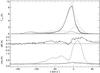 |
Fig. 11 Example of correction for stray radiation for a subregion in the NEP field. Upper panel: dashed curves show spectra taken at different LST (black and gray) with different stray radiation. Each curve is the average of 280 contiguous H i spectra on the Tmb scale; averaging is essential for lowering the noise, to reveal more clearly the effects of stray radiation. Dotted curves: our calculation of the expected stray radiation. Solid curves: spectra corrected for stray radiation, now well aligned. Middle panel: mean difference of the corrected spectra (note that the difference of the uncorrected spectra, or of the stray radiation, would be far offscale). Lower panel: spectra showing the rms of the 280 individual differences before (dashed) and after (solid) the correction for the stray radiation. |
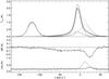 |
Fig. 12 Like Fig. 11, but based on 264 contiguous spectra in a subregion of N1. The stray correction at one LST is slightly too large, pushing the corrected spectrum slightly negative in the high-velocity wing. However, overall the correction is as effective as in the NEP example; note that the middle and lower panels are on the same scales as in Fig. 11. |
Examples of the stray radiation and our ability to remove it are shown in Figs. 11 and 12. Depending largely on where the spillover lobe is positioned on the sky, the stray radiation correction ranges in peak amplitude from a fraction of a K to several K. Most stray radiation tends to lie relatively close to zero velocity but is typically broader in velocity than the corrected/intrinsic spectra; the total velocity range over which stray radiation exceeds 0.1 K varies from a few tens of km s-1 to about 150 km s-1.
In these examples we compare spectra of the same region taken at different LST so that they will have different stray radiation. To reduce the noise and reveal the subtle changes after correction for stray radiation we have averaged many contiguous spectra that will have rather similar stray radiation. Figure 11 illustrates a case where there are large stray corrections that produce consistent results. For one of the epochs (gray lines in Fig. 11), the stray correction removes excess emission on both wings of the main peak, and the stray correction is significant all the way out to v ~ −120 km s-1. Compared to the up to 2 K differences in the uncorrected spectra, the difference between the corrected spectra is an order of magnitude smaller (middle panel). The difference after correction is not, however, zero, and some residual effects of stray radiation must still be present in the spectra.
Figure 12 provides another illustration from the N1 region, a region of low signal where the stray correction can have a relatively large effect on the derived line profile and its integral W. Here, for one observation (gray lines in Fig. 12) the stray correction overcorrects somewhat on either side of the main peak, yielding a slight dip below zero near v ~ 30 km s-1 and v ~ −60 km s-1. However, the stray correction still significantly reduces the difference between the two observations and the amplitude of the rms difference spectrum, as shown in the middle and lower panels of Fig. 12, respectively. Note that these panels are on the same scales as the corresponding panels in Fig. 11; the residual effects remaining in the corrected spectra are similar.
The quantification of the errors remaining because of imperfections in the stray radiation correction, and the cumulative effects on W, will be discussed further in Sect. 7.3 in the context of the other sources of error. Judging from many more comparisons of repeat measurements of different fields, the largest errors in the stray radiation correction tend to occur within a few tens of km s-1 of zero velocity, with a typical amplitude of 0.1 to 0.2 K, although in the worst cases the error can exceed 0.5 K.
7. Error estimates
In this section we evaluate the various contributions to the errors in the GBT H i spectra. The effects of errors are manifested in the non-reproducibility of measurements. Comparisons between spectra can be done on a channel by channel basis, T(v), or for a line integral W (in K km s-1) of T(v) over some velocity range. Because of different applications of H i spectra, it is relevant to address the errors for each metric.
7.1. Line noise
The individual survey spectra from Martin et al. (in prep.) have an rms noise in
emission-free channels of σ0 = 0.16 K. When the spectra are
interpolated into the data cube at Nyquist sampling this is reduced to
σ0 = 0.11 K (Mangum et al.
2007). The 21-cm line emission itself can significantly increase the noise at
velocities where it is bright:  (6)where
Tsys is the system temperature
(Tsys ≈ 20 K, Sect. 2).
For clarity, T(v) is referred to simply
as T for the remainder of this discussion.
(6)where
Tsys is the system temperature
(Tsys ≈ 20 K, Sect. 2).
For clarity, T(v) is referred to simply
as T for the remainder of this discussion.
All the GBT H i observations measure spectra in two orthogonal linear polarizations, labeled XX and YY, which should be receiving essentially identical 21-cm emission and identical stray radiation. Therefore, we are able to check the above equation by comparing spectra in the two polarizations. Both were processed in identical parallel streams prior to removal of distinct instrumental baselines. The difference in the baseline-subtracted XX and YY spectra provides a good indication of the error inherent in a single measurement. It eliminates the additional uncertainty arising from the stray radiation subtraction which is in common, but includes channel noise and baseline error. This difference would also reveal any mis-calibration of the two receiver channels and any real differences in the received H i signal because of differences in beam shape, pointing, or sidelobes. These latter effects, however, are thought to be small compared to the other error terms.
Because the errors in XX and YY are independent, and ultimately the XX and YY spectra are
averaged together to form
T = (TXX + TYY)/2,
the estimator of interest in assessing errors in T is the dispersion
σT, the standard deviation about the mean
of
ΔTpol = (TXX − TYY)/2.
Figure 13 displays this dispersion based on all of
our NEP spectra. The data over the v range of −50 km s-1 to
+ 25 km s-1 have been binned by T, each bin containing
2 × 10⁵ points. The T-dependence of the standard deviation
follows the prediction from Eq. (6),
overplotted in Fig. 13 using
 K as measured in the
individual spectra and a typical Tsys of 20 K.
K as measured in the
individual spectra and a typical Tsys of 20 K.
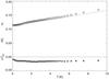 |
Fig. 13 Estimating the noise in a spectrum T using ΔTpol. Open circles give the standard deviation of ΔTpol within bins of 2 × 10⁵ data points as a function of T, using spectra from all NEP pointings. This agrees closely with the prediction (dotted line) from Eq. (6) with σ0 = 0.111 K and Tsys = 20 K. Also shown is the mean of ΔTpol for each bin. |
7.2. Baselines
The mean of the distribution of ΔTpol within each bin, also shown in Fig. 13, is slightly offset from zero, indicating a systematic difference in XX and YY that can be attributed to imperfect baseline removal. This offset – though well-characterized by a mean of −15 mK – does vary from spectrum to spectrum with a standard deviation of ~27 mK. This gives some sense of the size of the baseline error in the polarization-averaged spectrum T; it is so small compared to σ(v) that it has little effect on the dispersion described above. However, because a baseline error is systematic over many channels, it can accumulate as a significant error in W.
We illustrate this using the same NEP data, defining W to be the line
integral over Nch = 94 channels of width
Δv = 0.8 km s-1 over the range −50 km s-1 to
+25 km s-1. We calculated the dispersion
σW of
ΔWpol = (WXX − WYY)/2
for bins in W (2400 points each), plotting this in the upper part of
Fig. 14. The upper dashed line is a prediction of
this dispersion, combining in quadrature the minimal channel noise
 (dotted line) and a baseline
error of 0.027NchΔv (both in
K km s-1); note that the latter is now the larger contribution, because of
how it accumulates systematically. The larger values of W often result
from larger T and thus larger σ(v),
although this is not necessarily the case with very broad lines. The slight upward trend
in the observed dispersion toward larger W could therefore be a result of
the increasing contribution of σ(v) to the overall
error. For completeness, we show the mean of ΔWpol as well and
the prediction
−0.015NchΔv K km s-1.
(dotted line) and a baseline
error of 0.027NchΔv (both in
K km s-1); note that the latter is now the larger contribution, because of
how it accumulates systematically. The larger values of W often result
from larger T and thus larger σ(v),
although this is not necessarily the case with very broad lines. The slight upward trend
in the observed dispersion toward larger W could therefore be a result of
the increasing contribution of σ(v) to the overall
error. For completeness, we show the mean of ΔWpol as well and
the prediction
−0.015NchΔv K km s-1.
The uncertainty in W = (WXX + WYY)/2 should also be on the order of 2 K km s-1; for optically thin emission, this corresponds to an uncertainty of only 4 × 1018 cm-2 in column density. Note, however, how this varies with the number of channels used in the W integral; it should be determined self-consistently for the W appropriate to each different region or application.
An independent estimate of the baseline errors can be made directly from the third-order polynomial models used to fit the residual baselines in the spectra (3.3). A Monte Carlo analysis based on the uncertainties of the coefficients of the Legendre polynomials yields errors in W of ~0.7 K km s-1 over the same −50 km s-1 to + 25 km s-1 velocity range, suggesting that the errors derived from ΔWpol are an upper limit. For the remainder of this paper we adopt this upper limit as it includes potential systematic errors (e.g., offsets) between XX and YY which are not detectable in their average, W.
The good agreement between the data and the predictions in Figs. 13 and 14 indicates that we have a good understanding of the origins of the errors that arise from noise and instrumental baselines and that there are not large differences in the H i signal measured in the two polarizations of a single observation. However, we still need to assess the errors arising from the stray radiation correction (Sect. 7.3), and any other time-varying error contribution (Sect. 7.4).
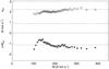 |
Fig. 14 Estimating the noise in the line integral W using ΔWpol. Open circles give the standard deviation of ΔWpol within bins of 2400 data points as function of W, using spectra from all NEP pointings as in Fig. 13. This agrees closely with the prediction (dashed line) based on the accumulation of line noise (dotted line) and baseline errors. Note that the baseline error is dominant in measurements of W, even though it is not dominant for measurements of the spectrum T (Fig. 13). Also shown are the data (filled circles) and the prediction (lower dashed line) for the mean ΔWpol. |
7.3. Stray radiation
As seen in the rms curves in Figs. 11 and 12, the baseline error and line noise are not the entire story. Changes that affect both XX and YY simultaneously and systematically can only be diagnosed with repeated observations at the same position.
The data from the NEP field, covering 44 100 spatial pixels three times each, are used
here to examine the reproducibility of spectra with a large range in T
and W. This allows us to assess how the uncertainty in the stray
radiation correction contributes to the overall error. To estimate the errors in a single
observation,
T = (TXX + TYY)/2,
for comparison with the results in the subsections above, we examine the statistics of
 ,
where i and j denote two separate observations, obtained
at different LST and elevation as this region was mapped over several months (2006/10 to
2007/01).
,
where i and j denote two separate observations, obtained
at different LST and elevation as this region was mapped over several months (2006/10 to
2007/01).
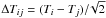
The dispersion of ΔTij for data binned (2 × 10⁵ per bin) in T, as in Sect. 7.1, is plotted as open circles in the upper part of Fig. 15 for each of the three observation pairs. The expected standard deviation from line noise (plus a minimal baseline component of 0.027 K added in quadrature) is plotted as a dashed line for Tsys = 20 K. Also shown as solid circles is the mean of ΔTij in each bin. We attribute both the excess of the observed dispersion above this prediction and the non-zero means to errors or imperfections in the stray radiation correction. A simplistic estimate of the total error can be obtained (crosses in Fig. 15) by including some fraction (here 6%) of the rms of the stray radiation corrections, in quadrature with the line noise.
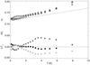 |
Fig. 15 Estimating the error in a spectrum T following stray radiation removal, using repeated observations in the NEP field. Open circles give the standard deviation of ΔTij within bins of 2 × 10⁵ data points as a function of T, using spectra from the three pairs of NEP observations (dark gray: 3−2, light gray: 1−3, black: 2−1). These lie slightly in excess of the prediction based on only line noise plus baseline errors (dashed line). Also shown is the mean of ΔTij for each bin for each ij combination. Both the excess and non-zero means arise from imperfect stray radiation removal. Crosses show a simple estimate of the total error which combines 6% of the rms spectrum of the stray radiation correction in quadrature with the line noise. |
The mean difference does vary from spectrum to spectrum with a standard deviation of
~0.041 K. This is about 40% of the typical dispersion in T attributed
to stray radiation. This gives some sense of the size of the systematic
error from the stray radiation correction (see also Figs. 11 and 12); it is small compared
to the dispersion of ΔTij but because it can
be systematic over many channels, it can accumulate as a significant error
in W. This is illustrated using the same NEP data. Again
defining W to be the line integral over
Nch = 94 channels of width
Δv = 0.8 km s-1 over the range −50 km s-1 to
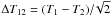
+25 km s-1, we calculated 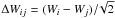 for bins (800 points) in W. As shown in Fig. 16, the mean of ΔWij is
typically <1.5 K km s-1 (lower points) across all
W bins. The dispersion in
ΔWij over all ij
combinations is plotted as open circles in the upper part of Fig. 16.
for bins (800 points) in W. As shown in Fig. 16, the mean of ΔWij is
typically <1.5 K km s-1 (lower points) across all
W bins. The dispersion in
ΔWij over all ij
combinations is plotted as open circles in the upper part of Fig. 16.
This analysis of observations of W in NEP, taken over a large range of time and with very different stray radiation corrections, indicate that the data are reproducible to an accuracy of 3 K km s-1 in a single mapping. This represents an accuracy of 1% to 3%, depending on W. As in Fig. 14, the dotted line in Fig. 16 is the predicted dispersion from channel noise alone, whereas the dashed line accounts for baseline errors as well. The upper dashed-dotted line is our prediction combining the channel noise in quadrature with a systematic error from the stray radiation correction of 0.041NchΔv. This systematic error includes both baseline and stray radiation errors as it is not possible to disentangle these here. The prediction is in close agreement with the observed dispersion.
 |
Fig. 16 Estimating the noise in the line integral W using ΔWij. Open circles give the standard deviation of ΔWij over all ij combinations within bins of 800 data points as a function of W, using repeated observations of spectra from all NEP pointings as in Fig. 15. This agrees closely with the prediction (dashed-dotted line) based on the accumulation of systematic errors in the stray radiation and baseline corrections added in quadrature with the line noise. The line noise and baseline errors (dotted and dashed lines from Fig. 14) are shown for comparison. Note that the error arising from the stray radiation and baseline correction is dominant in measurements of W, even though it is not dominant for measurements of the spectrum T (Fig. 15). Also shown are the data (filled circles) for the means ΔWij for each ij combination. |
The largest source of uncertainty in the stray radiation correction appears to be from incomplete knowledge of the sidelobe pattern for the telescope. Other sources of uncertainty in the stray radiation correction are discussed in Appendix D. Note that the velocity range used in this example was selected to accentuate errors from stray radiation. Because there is little significant stray contamination at |vLSR| ≫ 0 km s-1, measurements of W for intermediate and high-velocity H i components will have uncertainties closer to those predicted from the appropriate ΔWpol.
For high-latitude regions of very low Tb and W, the stray radiation from sidelobes overlapping H i near the Galactic plane can be as strong as the actual signal from the main beam at some velocities. The highest accuracy measurements can be obtained by timing the observations so that the spillover lobe does not lie near the bright H i in the Galactic plane, since that minimizes the stray radiation and the errors associated with its removal. With our knowledge of the extent and location of the sidelobes, we are able to determine the ideal LST range and successfully apply this strategy to the very faint ELAIS N1 field Martin et al. (in prep.).
7.4. Repeated observations of H I calibration standards
The long-term reproducibility of the GBT spectra can be gauged using our observations of standard H i calibration regions, S6 (Williams 1973, hereafter W73) and S8 (Kalberla et al. 1982, hereafter KMR), made over the period 2005/10 to 2008/03. The integration time for each spectrum obtained was 180 s and so these have much lower Tsys noise than the typical map spectra. Nevertheless they are affected by other sources of error, principally in the stray radiation correction. The spectra were reduced using the standard procedures (Sect. 4). For each region we created an average spectrum ⟨T⟩ from all the data.
There were 31 and 29 repeated observations of S6 and S8, respectively, each consisting of
two spectra, T1 and T2, from
consecutive 180 s integrations. The stray radiation correction, and also the baselines,
ought to be very similar for the two spectra in each pair. We therefore examined
 channel by channel. The standard deviation of ΔT12 for the
29 pairs in S8 is shown by the plus symbols in the lower part of Fig. 17, for channels in the velocity range used for the KMR calibration
(Sect. 8.1). As expected, this tracks closely the
prediction (dashed line) based on line noise alone from Eq. (6) with σ0 = 0.026 K as measured in
emission-free channels, and Tsys = 20 K.
channel by channel. The standard deviation of ΔT12 for the
29 pairs in S8 is shown by the plus symbols in the lower part of Fig. 17, for channels in the velocity range used for the KMR calibration
(Sect. 8.1). As expected, this tracks closely the
prediction (dashed line) based on line noise alone from Eq. (6) with σ0 = 0.026 K as measured in
emission-free channels, and Tsys = 20 K.
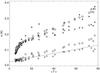 |
Fig. 17 Estimating the noise in the spectrum T of S8, using repeated observations. Plus symbols show the observed standard deviation of ΔT12 from channel by channel comparisons of two consecutive spectra, which ought to have very similar stray radiation and baselines. The measurements agree closely with the prediction (dotted line) from Eq. (6) for line noise alone. Open circles give the standard deviation of ΔTpol; these lie slightly above the prediction because of baseline errors. The filled circles give the standard deviation of ΔT = T − ⟨T⟩, which reflects all errors. As a prediction of this, the crosses show the result of adding 7% of the rms spectrum of the stray radiation correction in quadrature to the standard deviation of ΔTpol. The diamonds result from further addition of the effects of tiny 0.3% gain changes. The S8 data are consistent with errors in stray ~7% and scaling (e.g., gain) errors of <0.3%. |
As a second check, we examined the standard deviation of ΔTpol as in Fig. 13 (Sect. 7.1). These data are drawn as open circles in Fig. 17 and lie slightly above the dotted line because of baseline errors, which for these long integrations with lower Tsys noise have relatively more importance.
Next we examined the standard deviation of ΔT = T − ⟨T⟩. This is shown by the upper filled circles in Fig. 17. This somewhat larger dispersion (but note that it is still less than 1%) is from additional errors from the stray radiation corrections and potentially tiny changes of gain with time. We computed the rms spectrum of the actual stray radiation corrections and take some percentage of this as a rough estimate of what the error of the stray radiation correction might be. The crosses in Fig. 17 show the result of taking just 7% of the rms spectrum and adding this error estimate in quadrature to the other errors given by the standard deviation of ΔTpol. Although a simplistic description, it provides a reasonable explanation for both the magnitude of the standard deviation of ΔT and its dependence on ⟨T⟩.
Pursuing another approach that might reveal, for example, gain variations, we looked at the channel by channel correlation of T with ⟨T⟩, the slope of the regression being s. We carried out these regressions for data in the velocity ranges as defined by W73 and KMR for their calibration. By definition s will have a mean of unity, but it might vary from observation to observation due to various errors. Histograms of s are presented in Fig. 18. The standard deviations are 0.008 and 0.006 for S6 and S8, respectively. The GBT spectra are thus reproducible to better than 1% and thus any changes in gain are smaller than 1% as well. The smallest values of s occurred for observations taken during periods of rain, suggesting an additional source of atmospheric opacity not currently included in our reduction procedure; these outliers (one pair for S6 and two pairs for S8) were omitted in the above analysis of ΔT.
These two analyses of S8 are not decisive as to the presence of tiny secular changes in gain along with the errors from the stray radiation correction. S6 provides an opportunity to discriminate because the stray radiation is relatively weaker compared to the Tmb signal. Repeating the same analysis as for Fig. 17 for the case of S6, we found that the dispersion in ΔT, though smaller than in Fig. 17, is too large and has the wrong ⟨T⟩ dependence to be explained by an error of 5−10% of the rms stray radiation correction, suggesting that gain changes of order 0.5% might be present. In summary, a common explanation for S6 and S8 suggests gain changes of order 0.3% to 0.5% combined with stray correction error of size 7% of the rms stray radiation correction. The additional effect of 0.3% gain changes in S8, added in quadrature with the other errors, is illustrated by the diamonds in Fig. 17. We have also reproduced Fig. 18 for the case of S8 using simulated spectra starting with ⟨T⟩ and adding line noise, 7% of the rms stray radiation correction, and 0.3% gain changes with independent random seeds, verifying the self-consistency of this identification and quantification of the sources of error. Note that in the NEP (analysis in Fig. 15) and our other H i survey regions the signal Tmb is so small that any tiny gain errors would have a small effect.
This excellent reproducibility is to be contrasted to the assertions by Robishaw & Heiles (2009) that the GBT spectra suffer from 10% errors in the calibrated gain. Their analysis depended on solving simultaneously for gain and several parameters describing the amplitude of their adopted sidelobe pattern. However, their sidelobe pattern was only approximate, so that the resulting relatively large errors in the stray radiation correction become confused as implying significant changes in gain. We have seen such an ambiguity above, but at a level <1%, and our joint analysis for S6 and S8 via Figs. 17 and 18 is consistent with contributions from errors in the stray radiation correction and only tiny secular gain changes. The tiny gain changes found are consistent with what might be expected from the effects of gravitational and thermal distortions on the passive surface of the main paraboloid of the GBT, as described in Sect. 2.
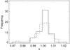 |
Fig. 18 The distribution of slopes s from regressions of T on ⟨T⟩ for S6 (dashed) and S8 (solid) from observations made over 2.5 years. The dispersions of 0.007 and 0.008, respectively, result from line noise, baseline errors, and errors in the stray radiation correction, and potentially from gain variations. |
7.5. Error budget and benefits from repeated observations
The contributions to the total error in the H i spectral data are summarized in Table 3 for both the T spectra and the integrated W. In the case that these errors are all independent, these can be added in quadrature to assess the total error.
Summary of errors in GBT H i spectral data.
Observations are often repeated to “beat down the errors”. This is certainly beneficial
for the errors arising from line noise and even for the baseline errors. However, it is
apparent that the dominant source of error in W for our NEP map is from
imperfect stray radiation removal. Furthermore, it is not clear how the dispersion of
ΔWij is to be interpreted in assessing the
errors in even a single observation. In the worst case, the measured dispersion could be
entirely due to the uncertainty in one of the observations, and so the uncertainty in that
single observation of W would be  times larger, on the order of 4 K km s-1 or up to a few percent of the values
typical in NEP. An error of this size corresponds to roughly 10% of the typical stray
radiation contamination for these NEP observations, compared to the estimated 7% in
Table 3. Note that additional observations will
not necessarily make the resulting average more accurate. One can hope that there will be
some cancellation, but it will depend on the accuracy of the stray radiation correction
for the times of observation.
times larger, on the order of 4 K km s-1 or up to a few percent of the values
typical in NEP. An error of this size corresponds to roughly 10% of the typical stray
radiation contamination for these NEP observations, compared to the estimated 7% in
Table 3. Note that additional observations will
not necessarily make the resulting average more accurate. One can hope that there will be
some cancellation, but it will depend on the accuracy of the stray radiation correction
for the times of observation.
8. Absolute calibration
8.1. Standard H I calibration directions
S8 at  is among the IAU primary
H i calibrators and has been studied extensively by KMR using the Effelsberg
100-m telescope. To compare our repeated GBT observations with KMR we computed the line
integral W over the prescribed velocity range
−5.1 < v < +22.3 km s-1,
finding WGBT = 831 ± 5 K km s-1, the standard
deviation being consistent with the expectation from Fig. 17. At the same angular resolution, KMR found
WEffel = 846 ± 14 K km s-1, the estimated error
combining a general scale uncertainty of 1.5% and an approximate 0.2 K systematic
uncertainty from their stray radiation correction. Thus
WEffel/WGBT = 1.018 ± 0.018.
We conclude that our independent calibration procedure produces 21-cm spectra in agreement
with this detailed previous calibration at the level of the uncertainties, 2%.
is among the IAU primary
H i calibrators and has been studied extensively by KMR using the Effelsberg
100-m telescope. To compare our repeated GBT observations with KMR we computed the line
integral W over the prescribed velocity range
−5.1 < v < +22.3 km s-1,
finding WGBT = 831 ± 5 K km s-1, the standard
deviation being consistent with the expectation from Fig. 17. At the same angular resolution, KMR found
WEffel = 846 ± 14 K km s-1, the estimated error
combining a general scale uncertainty of 1.5% and an approximate 0.2 K systematic
uncertainty from their stray radiation correction. Thus
WEffel/WGBT = 1.018 ± 0.018.
We conclude that our independent calibration procedure produces 21-cm spectra in agreement
with this detailed previous calibration at the level of the uncertainties, 2%.
S8 is a calibrator (along with the secondary calibrator S7) for the Leiden/Dwingeloo
Survey which forms the northern part of the LAB survey. The LAB resolution after
regridding the spatially-sampled data is about 40′ (Kalberla et al. 2005). To study changes in the spectrum with angular resolution,
KMR made a small 1° map sampled on a rectangular grid at 5′ intervals centred on S8.
Similarly, we made a  map with our standard scanning
setup. Errors from the stray radiation correction and baselines ought to be fairly uniform
over the map. Convolving our map to ever lower resolution, we reproduced the resolution
dependence found by KMR (their Fig. 5). From the GBT resolution to the LAB resolution,
W increases by a factor 1.017 ± 0.009. Using this to scale our pointed
observations gives W = 845 ± 9 K km s-1, to be compared to
849 ± 9 K km s-1 independently from our convolved small map, and
856 ± 14 K km s-1 found by KMR. The value computed from the LAB cube (with
the Wakker correction – see the following section) is 844 ± 12 K km s-1, in
close agreement at less than the 1% level.
map with our standard scanning
setup. Errors from the stray radiation correction and baselines ought to be fairly uniform
over the map. Convolving our map to ever lower resolution, we reproduced the resolution
dependence found by KMR (their Fig. 5). From the GBT resolution to the LAB resolution,
W increases by a factor 1.017 ± 0.009. Using this to scale our pointed
observations gives W = 845 ± 9 K km s-1, to be compared to
849 ± 9 K km s-1 independently from our convolved small map, and
856 ± 14 K km s-1 found by KMR. The value computed from the LAB cube (with
the Wakker correction – see the following section) is 844 ± 12 K km s-1, in
close agreement at less than the 1% level.
The other region that we measured repeatedly was S6 at
 .
Determining W over the range
−6.86 < v < +5.86 km s-1
(approximating W73; see KMR for a discussion) gives
WGBT = 289 ± 2 K km s-1. From a
scanned map we find that the
correction to the 35′ (40′) angular resolution of Hat Creek (LAB) is 0.990 ± 0.006
(0.993 ± 0.006) giving 286 ± 3 K km s-1 (287 ± 3). The value directly from the
convolved map is 289 ± 3 K km s-1 (290 ± 3). S6 is not a primary standard and
has not been measured as accurately as S8. W73 reports 299 ± 22 K km s-1 which
is probably systematically several percent high because it has not been corrected for
stray radiation. Within the large 7% uncertainty, it agrees with our measurement. The
value computed from the LAB data, interpolated to the S6 position, is
292 ± 5 K km s-1, again in close agreement with our measurements at the 2%
level.
.
Determining W over the range
−6.86 < v < +5.86 km s-1
(approximating W73; see KMR for a discussion) gives
WGBT = 289 ± 2 K km s-1. From a
scanned map we find that the
correction to the 35′ (40′) angular resolution of Hat Creek (LAB) is 0.990 ± 0.006
(0.993 ± 0.006) giving 286 ± 3 K km s-1 (287 ± 3). The value directly from the
convolved map is 289 ± 3 K km s-1 (290 ± 3). S6 is not a primary standard and
has not been measured as accurately as S8. W73 reports 299 ± 22 K km s-1 which
is probably systematically several percent high because it has not been corrected for
stray radiation. Within the large 7% uncertainty, it agrees with our measurement. The
value computed from the LAB data, interpolated to the S6 position, is
292 ± 5 K km s-1, again in close agreement with our measurements at the 2%
level.
8.2. Comparison with the LAB survey
For comparison with the LAB Survey, the GBT H i maps were convolved to the 40′ angular resolution of that survey. The convolution results in spectra with a negligible error from line noise, but any errors from the baseline and stray radiation corrections are not significantly reduced. For repeated observations of a region, we used the average spectrum.
Where the GBT observations completely cover a LAB beam, we interpolated the convolved GBT
data to the LAB positions in Galactic coordinates ( grid in l
and b) and to the slightly coarser velocity grid. The LAB and
convolved-GBT spectra almost always exhibited very similar spectral features, usually with
a small difference in overall scale. The line integral W is used to
quantify this scale; W is defined as the integral over all channels with
T > 1 K in either spectrum.
grid in l
and b) and to the slightly coarser velocity grid. The LAB and
convolved-GBT spectra almost always exhibited very similar spectral features, usually with
a small difference in overall scale. The line integral W is used to
quantify this scale; W is defined as the integral over all channels with
T > 1 K in either spectrum.
We performed a regression of WLAB on
WGBT, and since the LAB-survey-cube points at high Galactic
latitudes b are not independent, weights of cos b
were applied. This regression yields  (7)Wakker et al. (2011) has recommended that a Gaussian of peak amplitude
0.048 K, FWHM = 167 km s-1 (equivalent to 8.5
K km s-1 over the entire LAB velocity range), and center
v = −22 km s-1 be subtracted from all LAB
spectra. After making this “Wakker correction” to the LAB spectra we find
(7)Wakker et al. (2011) has recommended that a Gaussian of peak amplitude
0.048 K, FWHM = 167 km s-1 (equivalent to 8.5
K km s-1 over the entire LAB velocity range), and center
v = −22 km s-1 be subtracted from all LAB
spectra. After making this “Wakker correction” to the LAB spectra we find  (8)The intercept is now
significantly lower, and so our data support the application of the Wakker correction to
the LAB Survey data. The following analysis adopts this correction. However, note that
this correction is statistically based and might be different in different regions of the
survey and from spectrum to spectrum.
(8)The intercept is now
significantly lower, and so our data support the application of the Wakker correction to
the LAB Survey data. The following analysis adopts this correction. However, note that
this correction is statistically based and might be different in different regions of the
survey and from spectrum to spectrum.
If we adopt the hypothesis that the true intercept is zero, then  (9)We conclude that
overall the LAB scale is about 3% higher than for the GBT. This is taken into account in
the model H i sky used for stray radiation correction; see Appendix C.1.
(9)We conclude that
overall the LAB scale is about 3% higher than for the GBT. This is taken into account in
the model H i sky used for stray radiation correction; see Appendix C.1.
A single scale factor or a single intercept might be too simplistic. This is illustrated in Fig. 19 which shows the ratio WLAB/WGBT for every spectrum compared. In agreement with the conclusions of Higgs et al. (2005), we find that the LAB Survey appears to have random “calibration” errors, typically of a few percent. About 20% of the LAB spectra appear to be mis-scaled (up and down) by between 5% and 10% and another 7% of the spectra by more than 10%. There are a few very large outliers where a LAB spectrum has been mis-scaled by as much as 30%; these outliers were not included in the above analysis (though they are plotted in Fig. 19). Errors in the LAB Survey are discussed in more detail in Appendix D.2 (note that random LAB calibration errors tend to cancel out in the stray radiation calculation).
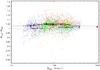 |
Fig. 19 WLAB/WGBT for every spectrum that could be compared (dots, color-coded by region). Filled circles show, for each of the observed regions, the weighted average ratio and its uncertainty (smaller than the filled circle for the typical uncertainty of ~0.004 in the regional averages), along with the region’s average WGBT and its dispersion (indicated by the horizontal errorbars). These comparisons suggest that a single scale factor (horizontal solid line, from Eq. (9)) might be too simplistic. |
Also shown in Fig. 19 are the weighted average ratios and their uncertainties for the 17 regions that we mapped, as obtained from regressions such as in Eq. (9) for each region. The differences from region to region are significantly more than the formal errors, suggesting that there might be systematic normalization errors of a few percent in the LAB survey data which vary with position in the sky. However, we have not found any systematic trend in the WLAB/WGBT ratio as a function of position.
Figure 19 does not show any clear trend of WLAB/WGBT or its dispersion vs. W. The S6 and S8 maps discussed above (Sect. 8.1) have the largest W values; based on six independent comparison positions in each of them, we find WLAB/WGBT = 1.015 ± 0.010 and 1.019 ± 0.007 for S6 and S8, respectively. Restricting the comparison to the four positions farthest from the GBT map edges reduces the ratios to 1.007 ± 0.008 and 1.010 ± 0.007, respectively. Though smaller than the overall ratio, these are still compatible with a 3% difference between LAB and GBT scales.
8.3. Comparison with Lyman-α measurements of H I
Using a sample of 28 bright QSOs and AGN as targets, Wakker et al. (2011) have compared measurements of the foreground Galactic NHI as determined by UV spectroscopy in the Lyman-α absorption line with measurements of NHI from 21-cm GBT observations in the same directions. The GBT data were reduced as described in this paper, and the correction for stray radiation was often significant. Third-order polynomials were fit to channels between −300 ≤ vLSR ≤ −150 km s-1 and + 100 ≤ vLSR ≤ + 200 km s-1. For some directions showing emission from high-velocity clouds the lower velocity range was changed to −300 ≤ vLSR ≤ −200 km s-1. Each 21-cm spectrum was examined for quality and a third-order polynomial baseline was found to be a good fit to the instrumental baseline. The ratio NHI(Lyα)/NHI(21 cm) = 1.00 ± 0.07 (1σ) indicating excellent agreement between the two entirely independent sets of measurements and independent tracers of H i. Some of the scatter must certainly result from structure in H i within the GBT beam as there is an enormous difference between the angular scales sampled by the UV absorption and 21-cm emission. We take this result as confirmation of the accuracy of our overall calibration procedure and an indication that the total error in GBT values of NHI must be significantly less than 7%.
9. Summary and conclusions
This paper describes the results of a program to develop a calibration procedure that allows accurate measurement of 21-cm H i spectra with the Green Bank Telescope of the NRAO. Using a combination of measurement and calculation we have developed a model for the all-sky response of the telescope and use it to correct for stray radiation in the GBT 21-cm spectra.
Several methods were used to estimate errors in the final spectra. Stochastic noise and instrumental baseline uncertainties are well understood and can be made quite low in long integrations (Sect. 7.1). The overall calibration to an absolute brightness scale appears to be correct to within a few percent as judged against measurements of standard radio continuum sources and the moon (Sect. 5).
The correction for stray radiation is the most uncertain, and can produce errors at any given velocity of as much as 0.5 K, though these occur mainly at |vLSR| ≲ 20 km s-1 (Sect. 6.5). Errors in the total W caused by errors in the stray radiation correction are typically less than 3 K km s-1 or 4 K km s-1 in the worst case (Sects. 7.3 and 7.5). These are equivalent to an error in optically thin NHI of ~5 × 10¹⁸ and 7 × 1018 cm-2. Overall the system is quite stable. We see no evidence for the “10% gain fluctuations” reported by Robishaw & Heiles (2009). An independent investigation of the H i content of nearby galaxies with the GBT (Hogg et al. 2007) achieved accuracies of 3.5%, where the main source of error was baseline uncertainties.
The corrected GBT data are in good agreement with other measurements of H i. Most interestingly, the GBT data give, on average, identical values of NHI as those derived from Lyman-α measurements towards a sample of AGN and QSOs (Wakker et al. 2011, and our Sect. 8.3). The GBT data also agree to within a few percent with previous measurements of “standard” H i calibration directions and with other H i observations at lower angular resolution. We have shown, however, that applying the “Wakker correction” to the LAB survey (Wakker et al. 2011) improves the agreement between that survey and the GBT spectra.
For the GBT at 1.42 GHz we find that 0.88 of the telescope’s response is within 1° of the
main beam, with most concentrated within  of the main beam, while another
0.098 ± 0.005 of the telescope’s response is in sidelobes more than one degree from the main
beam. We thus account for 0.978 ± 0.005 of the telescope’s response including that which
always lies on the ground, although the uncertainty of ± 0.005 applies
only to that part of the sidelobe that sees the sky: the part that sees only the ground
cannot be measured, only calculated. These results are very constrained. Given the
measurements of the sidelobes there are only two parameters that can be varied:
ηmb and ηsl. The value of
ηsl has been optimized from the observations (Sect. 6.1.3); any change in ηmb
would increase discrepancies with other measurements (Sect. 7). Attempts to add an isotropic component to the GBT beam pattern gave
unacceptable results for the stray correction, implying
ηiso < 0.01. Strictly speaking, only
the part of the isotropic component lying above the horizon is constrained by this analysis.
However, the magnitude of any extra component of P in a backlobe is also strongly
constrained by the low receiver Tsys. Given that our model
already has nearly 2% of P intersecting the ground, any additional component that lies on
the ground must have much less than 1% of the total P.
of the main beam, while another
0.098 ± 0.005 of the telescope’s response is in sidelobes more than one degree from the main
beam. We thus account for 0.978 ± 0.005 of the telescope’s response including that which
always lies on the ground, although the uncertainty of ± 0.005 applies
only to that part of the sidelobe that sees the sky: the part that sees only the ground
cannot be measured, only calculated. These results are very constrained. Given the
measurements of the sidelobes there are only two parameters that can be varied:
ηmb and ηsl. The value of
ηsl has been optimized from the observations (Sect. 6.1.3); any change in ηmb
would increase discrepancies with other measurements (Sect. 7). Attempts to add an isotropic component to the GBT beam pattern gave
unacceptable results for the stray correction, implying
ηiso < 0.01. Strictly speaking, only
the part of the isotropic component lying above the horizon is constrained by this analysis.
However, the magnitude of any extra component of P in a backlobe is also strongly
constrained by the low receiver Tsys. Given that our model
already has nearly 2% of P intersecting the ground, any additional component that lies on
the ground must have much less than 1% of the total P.
The calibration techniques are illustrated using data from H i maps made in connection with studies of interstellar dust and the cosmic infrared background (Martin et al., in press; Planck Collaboration et al. 2011a). Overall, the data reduction process described here reduces systematic uncertainties in GBT H i spectra by at least an order of magnitude. Extra precision might be obtained with a better model for the far sidelobes including the possibility of reflections from the ground, allowance for the slight changes in telescope geometry with elevation angle, and more detailed consideration of atmospheric opacity during periods of rain. Given the unblocked optics of the GBT it should be possible, in principle, to construct a receiver for 21-cm work with negligible forward sidelobes and a stray radiation component that is likewise negligible. This could be achieved in the near future with phased-array feed receivers (Landon et al. 2010; Jeffs et al. 2010).
Jim Braatz, October 30, 2009: Calibration of GBT Spectral Line Data in GBTIDL v2.1, from http://www.gb.nrao.edu/GBT/DA/gbtidl/gbtidl_calibration.pdf
This is the projected center as seen along the direction of the main beam, z; the projected aperture diameter is 100 m.
Acknowledgments
We thank Ron Maddalena, Rick Fisher, and Roger Norrod for many helpful discussions and Ron Maddalena for a critical reading of the manuscript. Bob Anderson supplied Fig. 3. We also thank the referee, Peter Kalberla, for his detailed reading and comments. The National Radio Astronomy Observatory is a facility of the National Science Foundation, operated under a cooperative agreement by Associated Universities, Inc. This work was supported in part by the Natural Sciences and Engineering Research Council of Canada.
References
- Albert, C. E., Blades, J. C., Morton, D. C., et al. 1993, ApJS, 88, 81 [NASA ADS] [CrossRef] [Google Scholar]
- Blagrave, K., Lockman, F. J., & Martin, P. G. 2010, in The Dynamic Interstellar Medium: A Celebration of the Canadian Galactic Plane Survey, ed. R. Kothes, T. L. Landecker, & A. G. Willis (San Francisco: ASP), 156 [Google Scholar]
- Boulanger, F., & Perault, M. 1988, ApJ, 330, 964 [NASA ADS] [CrossRef] [Google Scholar]
- Boulanger, F., Abergel, A., Bernard, J., et al. 1996, A&A, 312, 256 [NASA ADS] [Google Scholar]
- Dauger, D. E. 1996, Comp. Phys., 10, 591 [CrossRef] [Google Scholar]
- Dickey, J. M., McClure-Griffiths, N. M., Stanimirović, S., Gaensler, B. M., & Green, A. J. 2001, ApJ, 561, 264 [NASA ADS] [CrossRef] [MathSciNet] [Google Scholar]
- Goldsmith, P. F. 2002, in Single-Dish Radio Astronomy: Techniques and Applications, ed. S. Stanimirovic, D. Altschuler, P. Goldsmith, & C. Salter, ASP Conf. Ser., 278, 45 [Google Scholar]
- Green, D. A. 1993, MNRAS, 262, 327 [NASA ADS] [CrossRef] [Google Scholar]
- Hartmann, D. 1994, Ph.D. Thesis [Google Scholar]
- Hartmann, D., & Burton, W. B. 1997, Atlas of Galactic Neutral Hydrogen (Cambridge, UK: Cambridge University Press) [Google Scholar]
- Hartmann, D., Kalberla, P. M. W., Burton, W. B., & Mebold, U. 1996, A&AS, 119, 115 [NASA ADS] [CrossRef] [EDP Sciences] [Google Scholar]
- Hasinger, G., Burg, R., Giacconi, R., et al. 1993, A&A, 275, 1 [NASA ADS] [Google Scholar]
- Hauser, M. G., Arendt, R. G., Kelsall, T., et al. 1998, ApJ, 508, 25 [NASA ADS] [CrossRef] [Google Scholar]
- Heiles, C., & Wrixon, G. T. 1976, Meth. Exp. Phys., 12, 58 [CrossRef] [Google Scholar]
- Heiles, C., Kulkarni, S., & Stark, A. A. 1981, ApJ, 247, L73 [NASA ADS] [CrossRef] [Google Scholar]
- Heiles, C., Robishaw, T., Troland, T., & Roshi, D. A. 2003, A Preliminary Report: March 16, 2003 Calibrating the GBT at L, C, and X bands, NRAO GBT Comissioning Memo 23 [Google Scholar]
- Higgs, L. A., Landecker, T. L., Asgekar, A., et al. 2005, AJ, 129, 2750 [NASA ADS] [CrossRef] [Google Scholar]
- Hobbs, L. M., Morgan, W. W., Albert, C. E., & Lockman, F. J. 1982, ApJ, 263, 690 [NASA ADS] [CrossRef] [Google Scholar]
- Hogg, D. E., Roberts, M. S., Haynes, M. P., & Maddalena, R. J. 2007, AJ, 134, 1046 [NASA ADS] [CrossRef] [Google Scholar]
- Hovenac, E. A. 1989, Am. J. Phys., 57, 79 [NASA ADS] [CrossRef] [Google Scholar]
- Hunter, D. A., Zahedy, F., Bowsher, E. C., et al. 2011, AJ, 142, 173 [NASA ADS] [CrossRef] [Google Scholar]
- Jahoda, K., McCammon, D., Dickey, J. M., & Lockman, F. J. 1985, ApJ, 290, 229 [NASA ADS] [CrossRef] [Google Scholar]
- Jahoda, K., Lockman, F. J., & McCammon, D. 1990, ApJ, 354, 184 [NASA ADS] [CrossRef] [Google Scholar]
- Jeffs, B. D., Warnick, K. F., Landon, J., et al. 2010, in CALIM 2010, ASTRON, Dwingeloo The Netherlands, 22–27 August [Google Scholar]
- Kalberla, P. M. W., & Kerp, J. 2009, ARA&A, 47, 27 [NASA ADS] [CrossRef] [Google Scholar]
- Kalberla, P. M. W., Mebold, U., & Reich, W. 1980, A&A, 82, 275 [NASA ADS] [Google Scholar]
- Kalberla, P. M. W., Mebold, U., & Reif, K. 1982, A&A, 106, 190 [NASA ADS] [Google Scholar]
- Kalberla, P. M. W., Burton, W. B., Hartmann, D., et al. 2005, A&A, 440, 775 [NASA ADS] [CrossRef] [EDP Sciences] [Google Scholar]
- Kalberla, P. M. W., McClure-Griffiths, N. M., Pisano, D. J., et al. 2010, A&A, 521, A17 [NASA ADS] [CrossRef] [EDP Sciences] [Google Scholar]
- Keihm, S. J., & Langseth, M. G. 1975, Icarus, 24, 211 [NASA ADS] [CrossRef] [Google Scholar]
- Kerp, J., Winkel, B., Ben Bekhti, N., Floeer, L., & Kalberla, P. 2011, Astron. Nachr., 332, 637 [NASA ADS] [CrossRef] [Google Scholar]
- Kerr, F. J., Bowers, P. F., Jackson, P. D., & Kerr, M. 1986, A&AS, 66, 373 [NASA ADS] [Google Scholar]
- Kouyoumjian, R. G., & Pathak, P. H. 1974, Proc. Inst. Elec. Eng., 62, 1448 [CrossRef] [Google Scholar]
- Kuntz, K. D., & Danly, L. 1992, PASP, 104, 1256 [NASA ADS] [CrossRef] [Google Scholar]
- Landon, J., Elmer, M., Waldron, J., et al. 2010, AJ, 139, 1154 [NASA ADS] [CrossRef] [Google Scholar]
- Lee, S. H., & Ruddick, R. C. 1985, IEEE Trans. on Antennas and Propagation, AP-33, 189 [Google Scholar]
- Lee, S. H., Ruddick, R. C., Burnside, W. D., & Wang, N. 1979, IEEE AP-S International Symposium Digest, 1, 63 [Google Scholar]
- Lee, S. H., Ruddick, R. C., & Lambert, K. M. 1990, IEEE Trans. on Antennas and Propagation, AP-38, 889 [Google Scholar]
- Lockman, F. J., & Condon, J. J. 2005, AJ, 129, 1968 [NASA ADS] [CrossRef] [Google Scholar]
- Lockman, F. J., Jahoda, K., & McCammon, D. 1986, ApJ, 302, 432 [NASA ADS] [CrossRef] [Google Scholar]
- Mangum, J. G., Emerson, D. T., & Greisen, E. W. 2007, A&A, 474, 679 [NASA ADS] [CrossRef] [EDP Sciences] [Google Scholar]
- Nikolic, B., Prestage, R. M., Balser, D. S., Chandler, C. J., & Hills, R. E. 2007, A&A, 465, 685 [NASA ADS] [CrossRef] [EDP Sciences] [Google Scholar]
- Norrod, R., & Srikanth, S. 1996, A Summary of the GBT Optics Design, NRAO GBT Memo 155 [Google Scholar]
- Ott, M., Witzel, A., Quirrenbach, A., et al. 1994, A&A, 284, 331 [NASA ADS] [Google Scholar]
- Planck Collaboration 2011a, A&A, 536, A24 [Google Scholar]
- Planck Collaboration 2011b, A&A, 536, A18 [NASA ADS] [CrossRef] [EDP Sciences] [Google Scholar]
- Prestage, R. M., Constantikes, K. T., Hunter, T. R., et al. 2009, IEEE Proc., 97, 1382 [NASA ADS] [CrossRef] [Google Scholar]
- Puccetti, S., Capalbi, M., Giommi, P., et al. 2011, A&A, 528, A122 [NASA ADS] [CrossRef] [EDP Sciences] [Google Scholar]
- Robishaw, T., & Heiles, C. 2009, PASP, 121, 272 [NASA ADS] [CrossRef] [Google Scholar]
- Sheppard, C. J. R., & Hrynevych, M. 1992, J. Opt. Soc. Am. A, 9, 274 [NASA ADS] [CrossRef] [Google Scholar]
- Shull, J. M., Jones, J. R., Danforth, C. W., & Collins, J. A. 2009, ApJ, 699, 754 [NASA ADS] [CrossRef] [Google Scholar]
- Snowden, S. L., Hasinger, G., Jahoda, K., et al. 1994, ApJ, 430, 601 [NASA ADS] [CrossRef] [Google Scholar]
- Srikanth, S. 1993, Profile Corrugated Horn for the GBT: Prototype Design and Measurement, NRAO GBT Memo 98 [Google Scholar]
- Srikanth, S., King, L., & Norrod, R. 1994, in IEEE Antennas and Propagation Society International Symposium, AP-S. Digest Publication Date: 20–24 June 1994, 1, 54 [Google Scholar]
- Stark, A. A., Gammie, C. F., Wilson, R. W., et al. 1992, ApJS, 79, 77 [NASA ADS] [CrossRef] [Google Scholar]
- van Woerden, H., Takakubo, K., & Braes, L. L. E. 1962, Bull. Astron. Inst. Netherlands, 16, 321 [Google Scholar]
- van Zee, L., Maddalena, R. J., Haynes, M. P., Hogg, D. E., & Roberts, M. S. 1997, AJ, 113, 1638 [NASA ADS] [CrossRef] [Google Scholar]
- Wakker, B. P., Lockman, F. J., & Brown, J. M. 2011, ApJ, 728, 159 [NASA ADS] [CrossRef] [Google Scholar]
- Williams, D. R. W. 1973, A&AS, 8, 505 [NASA ADS] [Google Scholar]
- Wrixon, G. T., & Heiles, C. 1972, A&A, 18, 444 [NASA ADS] [Google Scholar]
Appendix A: Calculation of the GBT antenna pattern
The main beam and the sidelobes of the GBT at 1.40 GHz were calculated using a reflector antenna code developed at the Ohio State University. This code, called the Antenna Workbench (Kouyoumjian & Pathak 1974; Lee et al. 1979; Lee & Ruddick 1985; Lee et al. 1990), can be used to analyze single or multiple reflectors. It is capable of calculating both near-field and far-field radiation patterns. The theoretical approach is based on a combination of geometrical theory of diffraction (GTD) and aperture integration (AI) techniques. Typically, AI is used for computing the main beam and the near sidelobes while GTD is used for computing the far sidelobes including the backlobes. For near-field calculations, GTD is used in some cases for the whole region including the near axis region. In addition, the code has the conventional physical optics (PO) method option, where the currents on the reflector surface over a two-dimensional grid system are integrated to obtain the radiation pattern. The code usually uses the PO option for antennas with multiple reflectors. The Antenna Workbench was modified specifically for the large main reflector of the GBT. In the present analysis, the multiple reflector option using the PO technique was not used because it does not include edge effects and hence cannot compute the far sidelobes accurately.
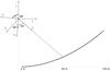 |
Fig. A.1 Geometry of the GBT used in Antenna Workbench calculations. SF and PF are the two foci of the ellipsoid of which the subreflector is a segment. PF is also the primary focus of the main parabolic reflector. The “s” coordinate system used for the near-field subreflector patterns is aligned with the zs axis running along the ellipsoid axis from PF toward SF. The illumination of the primary by these patterns is given in the “p” coordinate system, rotated with respect to “s”, so that the zp axis runs from PF toward the projected center of the primary. The all-sky far-field response is given in the non-subscripted coordinate system, where the z axis runs from PF in the direction of the main beam. All have y and z in the symmetric plane of the antenna. |
Figure A.1 shows the geometry of the primary and secondary reflectors of the GBT in the antenna symmetric plane that is vertical given the Alt-Az mounting. Three coordinate systems to be described further below are indicated. The non-subscripted one is associated with the primary, for the all-sky power pattern. That associated with the subreflector is subscripted “s”. A third coordinate system subscripted “p” is used for subreflector illumination of the primary, including for calculations of spillover past the primary. These are right-handed x − y − z systems, with the x axis directed up out of the page and yz in the antenna symmetric plane. In these coordinate systems we define φ to be the azimuthal angle (range −90° to 90°) around the z axis, measured relative to the x axis (φ = 0°) toward the y axis (φ = 90°). The polar angle θ is measured in half-planes of constant φ with an edge along z, relative to the z axis (θ = 0°) and ranging over 180° to the –z axis.
The radiation pattern of the GBT was computed in two steps. First, the pattern of the subreflector was calculated, in the “s” coordinate system whose origin is at one of the foci of the ellipsoid of which the subreflector is a segment. This focus is also the primary focus (PF) of the main reflector (Fig. A.1) and is the phase reference point for the subreflector patterns. The L-band feed horn is at the other focus of the ellipsoid, which is the GBT Gregorian (secondary) focus (SF). The zs axis runs from PF toward SF. These calculations used the measured far-field patterns of the L-band feed horn (Srikanth 1993) to illuminate the subreflector. The grids on the subreflector were set at 5 × 5 cm. Since the main reflector is in the near field of the subreflector, the near-field option in the code was used.
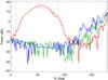 |
Fig. A.2 Subreflector near-field patterns in the “s” coordinate system as a
function of angle θs from the ellipsoid
axis zs, in half-planes with different
values of φs:
φs = −90°, red; 0°, green; 90°,
blue. Vertical lines indicate the near edge ( |


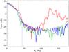 |
Fig. A.3 Subreflector illumination patterns on the main reflector as a function of angle
θp from
zp, the direction from PF to the
center of the primary, for three values of
φp in the main reflector (“p”)
coordinate system: φp = −90°, red;
0°, green; 90°, blue. Vertical lines indicate the near
( |

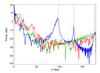 |
Fig. A.4 Calculated all-sky response of the GBT at 1.4 GHz, the main beam and far sidelobes,
as a function of angle from the main beam, θ, for three values of
φ in this coordinate system: φ = −90° (towards
the feed arm in the antenna symmetry plane), red; 0° (perpendicular to the antenna
symmetry plane), green; 90° (away from the feed arm), blue. To show details of the
sidelobes the scale has been magnified so that the forward gain of the main beam,
61.6 dBi at θ = 0° (Fig. 5,
Table 1), is beyond the range of this
figure. Vertical lines indicate the far edge
( |
Figure A.2 shows the power patterns calculated for
the subreflector in five φs half-planes.
Given the orientation of the “s” coordinate system, it is the patterns in
the half-planes approaching φs = −90° that
illuminate the main reflector. In this coordinate system, in the antenna symmetry plane
the near edge of the main reflector is at  and the far edge is at
 . At 54° is the center of the
main reflector3. The power pattern shown for
φs = −90° is appropriately peaked to
provide good illumination.
. At 54° is the center of the
main reflector3. The power pattern shown for
φs = −90° is appropriately peaked to
provide good illumination.
To calculate the illumination of the main reflector and the spillover past its edge,
these patterns were transformed from the “s” to the “p”
coordinate system with origin at PF and axis
zp oriented from PF to the projected center
of the 100-m main reflector (Fig. A.1). Figure A.3 shows the illumination of the main reflector from
the subreflector transformed to this coordinate system, for three different
φp half-planes. The edge of the main
reflector subtends an angle that varies between  and
and
 as
φp changes from −90° (far edge) to 90°
(near edge). As can be seen from both Figs. A.2
and A.3, the illumination taper in the antenna
symmetry plane at the far edge of the main reflector is about 5 dBi and somewhat lower,
−13 dBi, at the near edge, so that the spillover lobe from the main reflector is not
symmetrical around zp (see below).
as
φp changes from −90° (far edge) to 90°
(near edge). As can be seen from both Figs. A.2
and A.3, the illumination taper in the antenna
symmetry plane at the far edge of the main reflector is about 5 dBi and somewhat lower,
−13 dBi, at the near edge, so that the spillover lobe from the main reflector is not
symmetrical around zp (see below).
The second step was to determine the all-sky response of the GBT, expressed in the
non-subscripted coordinate system in Fig. A.1.
Subreflector patterns as calculated by Antenna Workbench for 72 half-planes in the range
of −90° ≤ φs ≤ 90° were used. The main
reflector was gridded into regions 30 × 30 cm, which is about 1.4λ,
adequate for the present work using AI. Far-field patterns were calculated at
 intervals in
φ and
intervals in
φ and  intervals in
θ. The computation of this pattern switches from AI to GTD at
intervals in
θ. The computation of this pattern switches from AI to GTD at
 where
Aw is the aperture diameter in wavelengths
in any given φ plane.
where
Aw is the aperture diameter in wavelengths
in any given φ plane.
Figure A.4 shows the main beam and the far
sidelobes of the GBT calculated for three different φ half-planes. The
on-axis (forward) gain is 61.61 dBi. An expanded view of the response near the main beam
is given in Fig. 5. The calculated half-power beam
width at 1.40 GHz is  , which differs from the
measured values by <1% and <2%,
respectively.
, which differs from the
measured values by <1% and <2%,
respectively.
The sidelobes stay mostly below -20 dBi. The peaks at about 10 dBi seen for φ = 90° at 5° and for φ = 0° at 13° are the spillover sidelobe from the subreflector (Appendix B.3). This can be appreciated in Figs. 8 and 9, noting that the –V axis there corresponds to φ = 90° and the H axis to φ = 0°.
The φ = 90° plane is in the symmetric plane of the GBT structure in the
direction away from the feed arm and so as θ increases the main reflector
is crossed. The two sidelobe peaks near 96° and 178° are caused by the spillover of the
subreflector illumination (Fig. A.3) past the far
edge ( ) and near edge
(
) and near edge
( ) of the main reflector,
respectively. Note that the former is stronger because as shown above the illumination
from the subreflector is larger at the far edge. This spillover lobe is manifested as an
asymmetrical ring around zp as
φp changes. The peak near
θ = 131°, which lies close to
zp (
) of the main reflector,
respectively. Note that the former is stronger because as shown above the illumination
from the subreflector is larger at the far edge. This spillover lobe is manifested as an
asymmetrical ring around zp as
φp changes. The peak near
θ = 131°, which lies close to
zp ( ), is caused by the diffracted
rays off the main reflector edge, similar to the backlobe that is observed on an on-axis
antenna. This is like the Arago spot from the subreflector discussed in Appendix B.2. Note that it is offset from the cone axis defining
the main reflector (
), is caused by the diffracted
rays off the main reflector edge, similar to the backlobe that is observed on an on-axis
antenna. This is like the Arago spot from the subreflector discussed in Appendix B.2. Note that it is offset from the cone axis defining
the main reflector ( ) to lower θ,
toward the far edge, because of the tilt of the reflector as seen from PF.
) to lower θ,
toward the far edge, because of the tilt of the reflector as seen from PF.
Appendix B: Calculation of diffraction from the subreflector using Fresnel diffraction theory
The primary reflector of the GBT is an offset segment of a symmetric parabola designed to eliminate aperture blockage and attendant sidelobes (Prestage et al. 2009). The Gregorian secondary subreflector is an offset section of an ellipsoid with the prime and secondary foci of the GBT at its two foci (Fig. A.1). The GBT L-band receiver feed horn is at the secondary focus. The geometric path from feed to subreflector to main reflector is clear of any obstruction. However, to a receiver feed that does not have a perfectly sharp cutoff of its field pattern at the subreflector edge, the subreflector appears as a blockage of the sky and so its diffractive effects must be considered. The GBT L-band feed does indeed somewhat over-illuminate (“spills over the edge of”) the subreflector, because a feed having a more sharply tapered beam pattern would be too large and heavy for the feed turret (Norrod & Srikanth 1996). Therefore the field pattern of the feed couples to the diffracted radiation, producing a modified Fresnel diffraction pattern, whose main “edge” feature is a set of annular peaks (rings) centered on the subreflector and beyond its projected edge. The dominant first ring is often called the “spillover sidelobe”. Here we present a calculation of the full power pattern.
B.1. Simple diffraction pattern of the subreflector
The shape of the subreflector is defined by the intersection of a cone, with apex at the secondary focus and an opening half-angle θH = 14.99°, with an offset ellipsoid of revolution (a prolate spheroid). As seen from the feed, the subreflector is to a first approximation a circular blockage defined by radius a = 3.775 m at distance d = 14.1 m from the secondary focus. At the operating wavelength of 21 cm, the secondary focus is in the near-field (d < a2/4λ) with respect to the subreflector and therefore satisfies the Fresnel condition. Furthermore, a4/d38λ < 1 so that the usual quadratic expansion of the phase used in the “Fresnel approximation” is valid (e.g., Sheppard & Hrynevych 1992; Dauger 1996). Thus the characteristics of the sidelobe pattern are closely related to the familiar near-field Fresnel diffraction by a circular blockage. This can be calculated for a receiving system with a plane wave arriving along the cone (negative zc) axis or, by reciprocity, for a transmitting system with an isotropic source at the feed. We have evaluated this from the analytic solution for a receiving system by Hovenac (1989) and obtained the same results numerically using the phasor approach described by Dauger (1996), in which reciprocity is implicit in the calculation. Dauger’s Fresnel Diffraction Explorer (FDE)4 can also be used to explore this interactively.
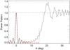 |
Fig. B.1 Radial profile of the familiar diffraction power pattern of a circular blockage, θ being with respect to the axis of the cone defining the subreflector. The vertical dashed line marks the edge of the subreflector as seen from the secondary focus. The dashed curve approximating the pattern near the central Arago spot is the lowest-order term in the analytic solution by Hovenac (1989). |
A radial profile of the axially-symmetric power pattern is shown in Fig. B.1. In this pattern, and in the GBT sidelobe pattern, there are two main phenomena of interest: (i) the finely-spaced ring structure near the cone axis with related modulations continuing at angles beyond the edge of the subreflector; and (ii) the coarser ring structure existing only beyond the edge. The existence of the diffraction spot on axis depends on interference of waves arising from all around the circumference of the subreflector in this circularly-symmetric geometry. On the other hand, the outer coarse ring structure is an “edge effect”, depending only locally on the sharp boundary, and so is qualitatively similar for a circular, square, or knife-edge configuration. As discussed below, the actual GBT sidelobe pattern shows the effects of three other factors: (i) the tapered beam of the L-band feed at the secondary focus; (ii) a screen (Fig. 3) adjacent to the subreflector edge in front of the supporting feed arm to redirect feed spillover; and (iii) the tilt of the subreflector.
B.2. The Arago spot
In the center of the diffraction pattern, at θ = 0, is the Arago (or
Poisson) spot, surrounded by a series of fine rings of comparable width. This pattern is
described accurately by the lowest-order term in the solution by Hovenac (1989), i.e., the square of the zero-order Bessel function of
the first kind,  , where
v = kar/d,
k = 2π/λ,
r is the radial coordinate in the image plane and
θ = arctan(r/d).
For the inner rings, the positions of the minima and maxima are near the zeros and peaks
of the function 1 + sin(2v), and thus at
(4n + zp)(π/4)/ka,
n = 1,2,... and
zp = −1 or 1, respectively. The first maximum is at
, where
v = kar/d,
k = 2π/λ,
r is the radial coordinate in the image plane and
θ = arctan(r/d).
For the inner rings, the positions of the minima and maxima are near the zeros and peaks
of the function 1 + sin(2v), and thus at
(4n + zp)(π/4)/ka,
n = 1,2,... and
zp = −1 or 1, respectively. The first maximum is at
 . In these units, the
half-power point of the main peak, at v = 1.1263, is at angle
1.434(π/4)/ka,
and so the FWHM of the Arago spot is
. In these units, the
half-power point of the main peak, at v = 1.1263, is at angle
1.434(π/4)/ka,
and so the FWHM of the Arago spot is
 ; this is inversely
proportional to a and, for fixed cone angle, also d.
The predicted FWHM and ring positions are in close agreement with the
properties of the actual scans of the GBT sidelobe using the Sun.
; this is inversely
proportional to a and, for fixed cone angle, also d.
The predicted FWHM and ring positions are in close agreement with the
properties of the actual scans of the GBT sidelobe using the Sun.
B.3. The main spillover sidelobe
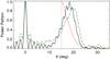 |
Fig. B.2 Solid (black): simulation of the effect of the tapered beam on the diffraction pattern, normalized to unity at the Arago spot. Step function (red): tapered field pattern of the L-band feed, relative to unity at the edge of the subreflector. Dashed (green): radial profile in the H direction through the observed sidelobe pattern. |
The dashed curve in Fig. B.2 shows the actual radial profile of the observed sidelobe through the Arago spot along the H direction. The oscillating coarse ring structure beyond the subreflector is an edge effect. However, the angular extent and amplitude are not the same as the pattern shown in Fig. B.1, because the strongly tapered feed pattern, already down 14.7 dB at the edge of the subreflector, does not illuminate the region beyond the edge of the subreflector uniformly. Thus the contribution to the diffraction pattern from radiation at large angles is strongly suppressed. We have simulated this as a steadily increasing “blockage” beyond the edge of the subreflector by implementing a method for treating variable transmission suggested by Dauger (1996). The amplitude and phase of the far-field pattern have been measured for the prototype L-band feed (Srikanth 1993) and as assumed in Appendix A should be approximately valid for the distance of the subreflector. The phase is roughly constant and we have taken the transmission (coupling) to decrease following the field pattern. The resulting diffraction pattern is shown in Fig. B.2, normalized to the amplitude of the Arago spot. The outer sidelobe pattern is systematically and differentially diminished: the peak intensity of the major spillover lobe compared to the Arago spot is lower and the outer rings are suppressed even more. As expected, the position of the peak of the major ring moves closer to the edge of the subreflector. These effects are evident in the observed sidelobe pattern, although the details are somewhat different; this might arise in part because of the large angles encountered in the actual GBT configuration.
B.4. Effects of the screen
The diffraction pattern is altered by the screen (Fig. 3) because it eliminates the contributions of interfering waves from a wedge with angular range φs ≈ 40° along the circumference of the subreflector centered on the positive V axis (away from the main beam). The amplitude of the Arago spot is reduced by a factor (1.−φs/360)2 ≈ 0.8. In the simulation for Fig. B.2 we have not included the screen; this would lower the Arago spot while leaving the major spillover lobe unaffected along the H profile thus bringing the relative deflections even closer to that observed.
Our calculations incorporating the screen indicate that in the profile along H the first fine ring is enhanced but in the orthogonal direction, along V, the ring amplitudes are reduced while the radial offset of the rings increases. These more subtle effects are discernable in the observations.
Because the spillover sidelobe is an edge effect, the disruption of the edge of the subreflector by the screen has a profound effect locally. This is clear in the observed pattern (see Figs. 8 and 9) where there is a bite out of the spillover ring pattern, about a 40° wedge out from the Arago spot at positive V centered on the feed leg. The screen apparently acts as an edge too, brightening the adjacent portion of the spillover sidelobe.
Superimposed on the inner edge of the observed main spillover lobe at negative V near H = 0, on the side of the main beam opposite to the direction of the screen, there is a pair of features in excess of the simple diffraction pattern (see Figs. 8 and 10). These have about the same beam integral as the portion of the major spillover lobe removed in the wedge, qualitatively consistent with conservation of energy. The screen has been well designed so that these features too lie well away from the main beam.
B.5. Effect of the tilt and motion of the subreflector
The required GBT geometry (Norrod & Srikanth
1996) is such that the subreflector is not quite perpendicular to the axis of
the cone, but rather tilted by
t =  ; relative to the defining
cone axis, the most distant edge is toward the main reflector and the direction of the
main beam (Fig. A.1). The semi-major axis, in the
antenna symmetric plane and joining the edges of the subreflector along the direction of
tilt, is of dimension 3.975 m, and the semi-minor axis is a = 3.775 m.
The distance along the cone axis from the secondary focus to the center of the minor
axis is then d = 14.1 m. These were the values of a
and d used above. The tilt shifts the position of the Arago peak
relative to the direction to the subreflector center, such that there is still
constructive interference between waves from the distant and near edges. Solving
Eq. (A7) of Dauger (1996), phases for the ends of
the major axis are equalized for an offset
; relative to the defining
cone axis, the most distant edge is toward the main reflector and the direction of the
main beam (Fig. A.1). The semi-major axis, in the
antenna symmetric plane and joining the edges of the subreflector along the direction of
tilt, is of dimension 3.975 m, and the semi-minor axis is a = 3.775 m.
The distance along the cone axis from the secondary focus to the center of the minor
axis is then d = 14.1 m. These were the values of a
and d used above. The tilt shifts the position of the Arago peak
relative to the direction to the subreflector center, such that there is still
constructive interference between waves from the distant and near edges. Solving
Eq. (A7) of Dauger (1996), phases for the ends of
the major axis are equalized for an offset  in the direction toward the
main beam. For the specified tilt, our estimate of the offset is
in the direction toward the
main beam. For the specified tilt, our estimate of the offset is
 . The angle between the
nominal cone axis defining the subreflector center and the main beam is
. The angle between the
nominal cone axis defining the subreflector center and the main beam is
 (Norrod & Srikanth 1996) at the rigging angle, elevation
 (Nikolic et al. 2007), the geometry used in the above calculations.
Thus the expected offset of the Arago spot at the rigging angle would be
(Nikolic et al. 2007), the geometry used in the above calculations.
Thus the expected offset of the Arago spot at the rigging angle would be
 along the
V axis above the main beam.
along the
V axis above the main beam.
At the rigging angle the main reflector is a perfect paraboloid to 21-cm radiation and the feed and subreflector are located optimally. At any other elevation angle, the main reflector deforms, displaces, and rotates while the feed and subreflector displace laterally in the symmetry plane, resulting in a slight misalignment of the optics (Srikanth et al. 1994). To track the primary focus position and maintain optimal efficiency together with precision pointing, the subreflector is moved to compensate (see, e.g., GBT Commissioning Memos 7 and 115). Thus the angle between the cone axis of the subreflector and the main beam changes slightly while tracking a source during an observation.
The elevation of the telescope when the Arago spot crossed the Sun during two different
nearly vertical scans was  and
and
 . Allowing for the change with
elevation we estimated that the position of the Arago spot would be at
. Allowing for the change with
elevation we estimated that the position of the Arago spot would be at
 . The two scans gave identical
observed offsets,
. The two scans gave identical
observed offsets,  . The good agreement is
perhaps fortuitous, given the complexity of the calculation.
. The good agreement is
perhaps fortuitous, given the complexity of the calculation.
B.6. Comments on the derived sidelobe model
These simple simulations reveal potential subtle issues regarding our method of deriving the sidelobe pattern by scanning it with the Sun. One involves the data reduction, where of necessity the scans have had a baseline removed. This introduces some uncertainty in the derived pattern. For example, in the area of the Arago spot there is a plateau not explained by the above simple diffraction theory (Fig. B.2). Even though this plateau is relatively weak, its subtended area could potentially lead to a significant contribution to the stray radiation. Another possibility, with an effect of the opposite sign, is that the derived pattern does not sink quite to zero in between the main spillover lobe and next minor rings. Again, because of the large area, even weak perturbations like this could have considerable power. To compensate for inadequate baseline removal, an approach could be to introduce a smooth parameterized sidelobe contribution centered on the subreflector and a function only of θ, e.g., a low order polynomial plus exponential. The parameters could be optimized during the procedure described in Sect. 6.1.2 to determine the optimal scaling of the sidelobe pattern. The effective coverage of different parts of the sky by the sidelobe pattern would therefore be reweighted.
A second issue concerns how the actual diffraction pattern might change in position with elevation of the telescope away from the rigging angle. As discussed in connection with the position of the Arago spot, displacement of the cone axis of the subreflector with respect to the main beam is difficult to calculate precisely but it might be several tenths of a degree over the range of elevations used in our survey, from 15° almost to the zenith. A smaller range was used in our mapping of the sidelobe pattern with the Sun. Because major features of the sidelobe pattern are related to subreflector spillover, and the latter is geometrically tied to the cone axis, the whole pattern can shift slightly with elevation. As a further complication, the screen is fixed to the feed arm, not moving with the subreflector during focus tracking. Thus the sidelobe pattern as measured and implemented will not be perfect; this might account (at least in part) for the slight differences among the optimal values of ηsl derived independently in different survey regions (Sect. 6.1.3) and for the stray radiation correction errors – which are nevertheless small (Sects. 7.3 and 7.4).
Appendix C: Stray radiation correction algorithm
The stray radiation correction is computed by evaluating the integral in Eq. (4). This is based on a program written in 1997 by Edward M. Murphy to correct stray radiation for H i spectra from the 43 m (140 ft) telescope at the NRAO incorporating a multi-component semi-analytic model developed from careful measurements of the 43 m telescope and its sidelobes (Murphy, 1993, unpublished M.A. Thesis, University of Virginia). For each input H i spectrum, an output spectrum of the estimated stray radiation was produced, with the input file serving as a template for the output file. The algorithm to estimate the sidelobe was straightforward, using an empirical model of the H i sky augmenting an early version of the Leiden-Dwingeloo survey with data from the Bell Labs survey and the Parkes 60-foot survey (Kerr et al. 1986; Stark et al. 1992; Hartmann & Burton 1997). This model sky had H i spectra at half-degree intervals in Galactic latitude l and longitude b. For each (l,b) point in the model, the date and time of the input spectrum were used to determine the corresponding position on the sky as viewed from the telescope. If this point lay above the horizon (it is assumed that there is no H i emission reflected from the ground; see Appendix D.3) and was more than one degree from the main beam, then the corresponding survey spectrum was multiplied by the relevant solid angle, by a factor to account for atmospheric absorption at the corresponding zenith angle, and by the sidelobe level at that position relative to the main beam. The appropriate velocity shift relative to the LSR was applied and the spectrum was spline-interpolated onto the input-spectrum velocity grid. The sum of all such weighted velocity-shifted spectra, looping over the grid of the model H i sky, was output as the stray radiation estimate. This computation of one stray-radiation spectrum required about one minute of CPU-time on a typical workstation.
C.1. Modified algorithm for the GBT
Major modifications to support calculation of stray radiation corrections specifically for the GBT involved four main areas: adding support for the SDFITS file format used for GBT observations, modifying the sky position algorithms to account for the fact that the GBT has an altitude-azimuth mount instead of the equatorial mount of the 43 m telescope (as well as including the horizon as seen from the GBT), modifications to speed up the calculation by a couple of orders of magnitude, and finally obtaining a good map of the GBT sidelobes (Sect. 6) which is stored in and interpolated from a 2-D array.
For the empirical model H i sky we adopted the LAB all-sky survey (Kalberla et al. 2005) after first subtracting a Gaussian with peak amplitude 0.048 K, center at −22 km s-1, and FWHM = 167 km s-1 from each LAB spectrum (the so-called “Wakker correction”, Wakker et al. 2011) and then dividing by a scale factor 1.0288, as discussed in Sect. 8.2 (see Eq. (9)). The “Wakker correction” to the LAB survey has a very small effect on the calibrated GBT spectra as it enters scaled by ηsl times the fraction of ηsl that is above the horizon. As the product of these quantities is always <0.1, its effect on calibrated GBT spectra is always <0.005 K.
Air mass measurements were available for NRAO at 5° intervals in elevation
angle el for 0° ≤ el ≤ 90° and at
15 intervals
for 0° ≤ el ≤ 15° (Maddalena 2005, priv. comm.: the air mass
measurements were actually performed nearby at Hot Springs, VA, on 15 June 2005). These
measurements were used to obtain the atmospheric optical
depth τatm as a function of el: a zenith
optical depth at 1420 MHz of τzenith ≈ 0.01, and an air mass
of roughly 31 at the horizon, implies that τatm ≈ 0.32 at
el = 0° (rather than becoming infinite there). However, as the sky at
el < 1° is obscured by hills around most of
the horizon, the improved atmospheric absorption values had little effect on the
calculated stray radiation. Information on the exact weather conditions is not used at
present when calculating the opacity, though there are indications in our data that rain
can add an extra opacity that might be accounted for in the future (Sect. 7.4; Maddalena, priv. comm.). Snow might also have a
significant effect both with its precipitation and with its accumulation in the GBT dish
– any effects from the latter not being sufficiently predictable to be corrected for.
However, variations in atmospheric pressure, temperature, and humidity are expected to
have very little effect on the atmospheric absorption; this is confirmed by the fact
that the repeated observations of S6 and S8 (Sect. 7.4) show no evidence for a systematic summer-vs.-winter effect.
Refraction results in more of the sky being visible to the telescope, an extra strip
approximately  wide around the horizon.
Effects of temperature, pressure, and humidity are included in the
refraction calculations. Inclusion of refraction typically changes the calculated stray
radiation by less than 1%, but up to 10% in extreme cases.
wide around the horizon.
Effects of temperature, pressure, and humidity are included in the
refraction calculations. Inclusion of refraction typically changes the calculated stray
radiation by less than 1%, but up to 10% in extreme cases.
For integration times of a few minutes or more, there are significant changes in the position of the sky relative to the horizon and, for the GBT, in the rotation of the sidelobe beam relative to the sky with accompanying changes in the Doppler shift of the stray radiation being accumulated. For an integration time of 120 s, such as we used for “staring observations” as opposed to on-the-fly mapping, calculating the sky, horizon, and beam positions at the middle of the time interval (rather than the beginning) yields typical improvements of a fraction of a percent though in extreme cases it can be 10%. To allow for even longer integration times, calculation of stray radiation contributions at multiple times within a single observation is supported.
The calculation was sped up mainly by two modifications. First, speed-up by nearly an
order of magnitude was obtained simply by using linear rather than spline interpolation
in velocity for the spectrum being accumulated. Second, another order of magnitude was
obtained by introducing a four-level tiling tree for the model sky spectra: a four-level
tesselation of the sky. The deepest level corresponds to independent spectra in roughly
 areas on the sky, appropriate
to the LAB survey sampling. Near the Galactic equator, these tiles are at
05 intervals
in b and l, i.e., the LAB grid. Near the Galactic
poles, LAB spectra at multiple l values were averaged together to
create tiles with widths on the sky of at
least 025 but no more
than 05. The next
level up, coarser tiles of roughly 1° × 1°, comprised of averages (weighted by solid
angle) of four (or, near the poles, sometimes three) of the lowest-level spectra.
Similarly, two further higher tiling levels of roughly 2° × 2° and 4° × 4° were
obtained. The loop over the tiles of the model starts at the highest 4° × 4° level.
Since much of the sidelobe area is quite smooth, this tiling made it possible to reduce
greatly the number of spectra that had to be accumulated for each stray calculation.
Where the sidelobe varied significantly on length scales smaller than the relevant tile,
or where part of the tile would be below the horizon or adjacent to the main beam, the
appropriate tiles on the levels below were traversed instead. The magnitude of the
introduced errors was estimated by computing stray radiation corrections for a random
sample of positions, dates, and LST values. For these modifications that yield faster
sidelobe spectrum evaluation, the resulting errors are small (rms 0.2%, max 3% of the
stray correction).
areas on the sky, appropriate
to the LAB survey sampling. Near the Galactic equator, these tiles are at
05 intervals
in b and l, i.e., the LAB grid. Near the Galactic
poles, LAB spectra at multiple l values were averaged together to
create tiles with widths on the sky of at
least 025 but no more
than 05. The next
level up, coarser tiles of roughly 1° × 1°, comprised of averages (weighted by solid
angle) of four (or, near the poles, sometimes three) of the lowest-level spectra.
Similarly, two further higher tiling levels of roughly 2° × 2° and 4° × 4° were
obtained. The loop over the tiles of the model starts at the highest 4° × 4° level.
Since much of the sidelobe area is quite smooth, this tiling made it possible to reduce
greatly the number of spectra that had to be accumulated for each stray calculation.
Where the sidelobe varied significantly on length scales smaller than the relevant tile,
or where part of the tile would be below the horizon or adjacent to the main beam, the
appropriate tiles on the levels below were traversed instead. The magnitude of the
introduced errors was estimated by computing stray radiation corrections for a random
sample of positions, dates, and LST values. For these modifications that yield faster
sidelobe spectrum evaluation, the resulting errors are small (rms 0.2%, max 3% of the
stray correction).
Appendix D: Uncertainties not related to the GBT response pattern
D.1. Undersampling in the LAB survey
The correction for stray radiation relies on the LAB survey to provide a 21 cm
Tb over the entire sky visible from Green Bank. The main
contribution to the LAB survey for the part of the sky seen by the GBT is the
Leiden-Dwingeloo (LD) H i survey that consists of observations spaced
 on the sky at an angular
resolution of 35′ (Hartmann & Burton
1997). It is sometimes said that the undersampling makes the LD survey equivalent
to a survey with an angular resolution of order 1°, but this is not correct.
Because of the undersampling, the LD survey (and hence the LAB in the North) cannot be
used for accurate interpolation between the measured positions – information at spatial
frequencies that are resolvable to the Dwingeloo antenna are aliased into lower spatial
frequencies biasing our estimate of the H i sky. At present there is no remedy
for this and it contributes an unknown error to the stray radiation correction. A new
H i survey of the northern sky is underway that should provide a much more
accurate, complete, data set from which to calculate the stray component in GBT spectra
(Kerp et al. 2011).
on the sky at an angular
resolution of 35′ (Hartmann & Burton
1997). It is sometimes said that the undersampling makes the LD survey equivalent
to a survey with an angular resolution of order 1°, but this is not correct.
Because of the undersampling, the LD survey (and hence the LAB in the North) cannot be
used for accurate interpolation between the measured positions – information at spatial
frequencies that are resolvable to the Dwingeloo antenna are aliased into lower spatial
frequencies biasing our estimate of the H i sky. At present there is no remedy
for this and it contributes an unknown error to the stray radiation correction. A new
H i survey of the northern sky is underway that should provide a much more
accurate, complete, data set from which to calculate the stray component in GBT spectra
(Kerp et al. 2011).
D.2. Errors in the LAB survey
Any errors in the LAB survey spectra will propagate through the stray radiation correction, reduced in their effect by ηsl = 0.0981 and the fractional solid angle of the erroneous spectra, and by the fact that multiple errors in opposite directions might cancel out. We consider here errors in the LAB survey discovered earlier (Higgs et al. 2005) and during the course of this work.
As discussed in Sect. 8.2, a very few of the LAB survey spectra have normalization errors of up to about 30%, but only a small fraction of the spectra appear to have normalization errors even at the ten percent level.
As noted earlier by Higgs et al. (2005) when
they compared their DRAO 26-m data to the LAB survey, a very few LAB spectra have large
spurious features. These are detected by comparison of LAB with other data; the fact
that it is the LAB feature that is spurious is indicated by the fact that (1) the
feature appears in the LAB spectrum but not in the other data; (2) nor does the feature
appear in LAB spectra at adjacent latitudes; and (3) the feature often has a shape that
is not typical of any real feature. (Note that LAB survey spectra at adjacent
longitudes are not independent at high latitudes, where a spurious
feature might thus propagate with varying intensity across several longitude points.)
Only where alternative data are available can the above errors be reliably detected and
corrected. This alternative is available for only 13 165 of the 257 762 LAB spectra; in
125 of these 13 165 spectra, a total of 141 spurious features were found (including 33
in the regions surveyed by Higgs et al. 2005).
Most were small, “dips” or “peaks” with a width of about 2 km s-1
superimposed on real features an order of magnitude larger in both width and height.
However, 6 of the LAB spectra had very wide spurious “peaks” at negative velocities. The
LAB spectrum at  has a “peak” over the
range
−300 km s-1 < v < −160 km s-1,
with a plateau of height 3.6 K in the range
−240 km s-1 < v < −190 km s-1
(this region should be zero); this feature also shows up at l = 139°
and
has a “peak” over the
range
−300 km s-1 < v < −160 km s-1,
with a plateau of height 3.6 K in the range
−240 km s-1 < v < −190 km s-1
(this region should be zero); this feature also shows up at l = 139°
and  , albeit with lower amplitudes
of 0.5 and 0.1 K, respectively. The LAB spectrum at
, albeit with lower amplitudes
of 0.5 and 0.1 K, respectively. The LAB spectrum at
 has a
peak of height 0.6 K in
−190 km s-1 < v < −70 km s-1
(this region should be zero). Finally, the two LAB spectra at (l = 132°
and
has a
peak of height 0.6 K in
−190 km s-1 < v < −70 km s-1
(this region should be zero). Finally, the two LAB spectra at (l = 132°
and  have a peak of height 2 K
in
−240 km s-1 < v < −20 km s-1
(the convolved GBT spectra, and adjacent LAB spectra, have three narrower peaks in this
velocity range, with heights of about 0.2 K). Replacing the spurious features by a
linear interpolation over the relevant velocity range works very well, except in the
last two cases (where convolved GBT spectrum values can be used instead, in the relevant
velocity region).
have a peak of height 2 K
in
−240 km s-1 < v < −20 km s-1
(the convolved GBT spectra, and adjacent LAB spectra, have three narrower peaks in this
velocity range, with heights of about 0.2 K). Replacing the spurious features by a
linear interpolation over the relevant velocity range works very well, except in the
last two cases (where convolved GBT spectrum values can be used instead, in the relevant
velocity region).
The existence of spurious LAB features and random LAB calibration errors in our large GBT fields allows for some quantification of the potential propagated error. For pointings near the middle of these fields, the major contribution to the stray radiation comes from the LAB spectra that were corrected for the above two types of errors, and comparing these cases to computations without these corrections indicates that these spurious features and mis-calibrations introduce errors of at most a few percent in the computed stray radiation correction. Thus any such spurious features that cannot be corrected (i.e., in regions with no comparison data) are not expected to contribute significant errors to the stray radiation computation.
D.3. Errors from the stray-correction algorithm
The program currently assumes that no 21-cm radiation is picked up through reflection from the ground; the tree-covered mountains around the GBT can be assumed to be good absorbers, but the fields in the immediate vicinity of the telescope might have a non-trivial albedo especially when wet. This was found to be the case for the moors around Dwingeloo (Hartmann et al. 1996). However, as the dominant GBT sidelobes are near and above the main beam (Fig. 8), the fraction of the response lying on the ground is at most a few percent and so the effect of reflections should be quite small.
The “sidelobes” over which the stray radiation is accumulated are considered to begin a degree from the center of the beam. Shifting this cutoff from a 1.0° radius to 0.9° has an effect of rms 2% (max 14%) on the stray radiation, according to a set of random test cases. Such effects are expected to be most significant when the GBT beam is pointed at a region with extended strong signals, such as the Galactic plane. For pointings in regions of low signal, even much larger changes in the definition of where the sidelobes begin have little effect.
As discussed above (Sect. B.6), variations in the geometry of the optics with telescope elevation angle can shift the sidelobe pattern by several tenths of a degree (its shape and amplitude pattern might also change slightly). This is at least an order of magnitude smaller than the angular scale on which the sidelobes vary, but could nonetheless lead to significant stray radiation errors for cases where the mean sky brightness is varying significantly at the edge(s) of the spillover lobe. Typically, such errors would be expected to be no more than a few percent of the calculated stray radiation; but in extreme cases, this effect could be larger. The present stray-correction algorithm ignores this telescope elevation effect, but in principal measurements might allow at least a partial correction for it.
For pointings in bright complex regions, spectra obtained at different times might change by a few percent due to the rotation relative to the sky of the slightly asymmetric main beam and inner sidelobes within 1.0° radius. Such “near-beam” effects cannot be corrected by this program due to the coarse grid of the all-sky LAB survey. This could be approached as a deconvolution problem using the accurately known near beam if a small fully sampled map were obtained quickly with the GBT. Given our interest in high latitude emission, this has not been pursued here.
All Tables
Calculated fractional power pattern at 1.4 GHz as a function of angle from the beam center.
All Figures
|
Fig. 1 The Green Bank Telescope in a view that shows its unblocked 100-m diameter aperture. |
| In the text | |
|
Fig. 2 The focal area of the GBT as seen from the surface of the main reflector, showing outlined in red, bottom to top, (i) the receiver room; with (ii) the L-band feed horn pointing upward at (iii) the 8-m subreflector. Just below the lower edge of the subreflector the lower portion of a screen is visible. This functions to direct feed spillover radiation that would otherwise strike the telescope arm back into the main reflector and onto the sky. |
| In the text | |
|
Fig. 3 The GBT subreflector and feed arm seen from the secondary focal point atop the receiver room. The screen redirects feed spillover away from the arm and down into the main reflector. |
| In the text | |
|
Fig. 4 Brightness temperature spectrum from the North Ecliptic Pole (NEP) data cube at
|
| In the text | |
|
Fig. 5 GBT antenna gain above isotropic for the main beam and near sidelobes at 1.4 GHz, as a function of polar angle θ from the main beam in several planes defined by φ (see Appendix A for the antenna code used for this calculation). The forward gain is 61.6 dBi (Table 1). |
| In the text | |
|
Fig. 6 Mapping the GBT sidelobe pattern using the Sun. Heavy lines indicate the position of the Sun relative to the main beam during the scan. Thin magenta lines indicate scans reflected in the beam’s line of symmetry (i.e., with the H coordinate replaced by −H). Dotted lines at high H show measurements that were not used because they showed no visible sidelobes above the noise. The center of the subreflector is 12.3° above the main beam. |
| In the text | |
|
Fig. 7 Estimating the optimal value of ηsl using three repeated observations at more than 4 × 10⁴ positions near the NEP, each repeat having different stray radiation. For different assumed ηsl, the difference between each observation of W and the mean of the three was calculated for every position. Histograms of the resulting distributions of differences show the sensitivity to ηsl, including the dotted curve for no stray radiation correction. Correction is clearly beneficial, and a minimum dispersion occurs for ηsl ≈ 0.097. Note that the dispersion does not quite reach the minimum predicted from line noise and baseline uncertainties alone (dashed line, see Sect. 7.2). |
| In the text | |
|
Fig. 8 Contours of the measured GBT far sidelobe gain G, relative to isotropic. The main beam is at the origin (indicated by the solid dot), and would peak at + 61.6 dBi. The H and V coordinates are the same as in Fig. 6. Elevation increases upward in the plot and the direction to the center of the subreflector is at V = 12.3°. The main “spillover lobe” is outlined by the yellow 0 dBi contour, with the blue 4 dBi and magenta 5 dBi contours defining its ridge; curving as a ring from below the main beam at (H,V) ~ (0°, −7°), it extends to about (H,V) ~ (12°,28°), beyond which it is blocked by the screen on the telescope arm (note that this blockage also yields a ridge stretching upward from the subreflector center along the edge of the gap at an angle about 35° from the vertical; this ridge passes through the end of the spillover lobe). Complementary to this missing part of the spillover lobe caused by the screen are the twin peaks below the main beam, at (H,V) ~ (± 1°, −3°), visible in the heavy black 10 dBi and thin gray 15 dBi contours. Outside the spillover lobe are three lower-amplitude rings (at radii θ ~ 26°, 29.5°, and 33° from the subreflector center). Inside is the Arago spot and surrounding rings centred at 11.879° on the axis above the main beam. Some features are easier to see in the 3Dplots of Figs. 9 and 10. Outside the faint spillover rings and outside the region (| H| < 35°,20° < V < 53°), the sidelobe levels are taken from the antenna code calculations. |
| In the text | |
|
Fig. 9 GBT response pattern P, as measured from scans of the Sun, on a linear scale. The H and V coordinates are the same as in Figs. 6 and 8. Note that this plot has been rotated so that its features are more easily visible – the vertical coordinate V increases from left to right in this figure. The truncated peak at center-left in this figure comprises both the main beam at (H,V) = (0,0) and the double-peak feature at (H,V) ~ (± 1°, −3°); the peak of the main beam would be far offscale at P = 1.12 × 10⁵. Near the center of the spillover lobe, the Arago spot is visible. The gap at high V in the spillover lobe and its surrounding rings arises from the presence of the reflecting screen at the subreflector edge. |
| In the text | |
|
Fig. 10 Measured GBT response pattern P, as in Fig. 9, but for sidelobes closer to the main beam. The Arago spot, peaking at ≈ 0.25, is visible at the right, along with its surrounding rings. The double-peak feature at (H,V) ~ (±1°, −3°) appears just to the left of the (truncated) main beam, with height P ≈ 2.6. This contains the power scattered from the forward spillover lobe by the reflecting screen on the feed arm (Fig. 3). The peak of the main beam would be far offscale at P = 1.12 × 10⁵. |
| In the text | |
|
Fig. 11 Example of correction for stray radiation for a subregion in the NEP field. Upper panel: dashed curves show spectra taken at different LST (black and gray) with different stray radiation. Each curve is the average of 280 contiguous H i spectra on the Tmb scale; averaging is essential for lowering the noise, to reveal more clearly the effects of stray radiation. Dotted curves: our calculation of the expected stray radiation. Solid curves: spectra corrected for stray radiation, now well aligned. Middle panel: mean difference of the corrected spectra (note that the difference of the uncorrected spectra, or of the stray radiation, would be far offscale). Lower panel: spectra showing the rms of the 280 individual differences before (dashed) and after (solid) the correction for the stray radiation. |
| In the text | |
|
Fig. 12 Like Fig. 11, but based on 264 contiguous spectra in a subregion of N1. The stray correction at one LST is slightly too large, pushing the corrected spectrum slightly negative in the high-velocity wing. However, overall the correction is as effective as in the NEP example; note that the middle and lower panels are on the same scales as in Fig. 11. |
| In the text | |
|
Fig. 13 Estimating the noise in a spectrum T using ΔTpol. Open circles give the standard deviation of ΔTpol within bins of 2 × 10⁵ data points as a function of T, using spectra from all NEP pointings. This agrees closely with the prediction (dotted line) from Eq. (6) with σ0 = 0.111 K and Tsys = 20 K. Also shown is the mean of ΔTpol for each bin. |
| In the text | |
|
Fig. 14 Estimating the noise in the line integral W using ΔWpol. Open circles give the standard deviation of ΔWpol within bins of 2400 data points as function of W, using spectra from all NEP pointings as in Fig. 13. This agrees closely with the prediction (dashed line) based on the accumulation of line noise (dotted line) and baseline errors. Note that the baseline error is dominant in measurements of W, even though it is not dominant for measurements of the spectrum T (Fig. 13). Also shown are the data (filled circles) and the prediction (lower dashed line) for the mean ΔWpol. |
| In the text | |
|
Fig. 15 Estimating the error in a spectrum T following stray radiation removal, using repeated observations in the NEP field. Open circles give the standard deviation of ΔTij within bins of 2 × 10⁵ data points as a function of T, using spectra from the three pairs of NEP observations (dark gray: 3−2, light gray: 1−3, black: 2−1). These lie slightly in excess of the prediction based on only line noise plus baseline errors (dashed line). Also shown is the mean of ΔTij for each bin for each ij combination. Both the excess and non-zero means arise from imperfect stray radiation removal. Crosses show a simple estimate of the total error which combines 6% of the rms spectrum of the stray radiation correction in quadrature with the line noise. |
| In the text | |
|
Fig. 16 Estimating the noise in the line integral W using ΔWij. Open circles give the standard deviation of ΔWij over all ij combinations within bins of 800 data points as a function of W, using repeated observations of spectra from all NEP pointings as in Fig. 15. This agrees closely with the prediction (dashed-dotted line) based on the accumulation of systematic errors in the stray radiation and baseline corrections added in quadrature with the line noise. The line noise and baseline errors (dotted and dashed lines from Fig. 14) are shown for comparison. Note that the error arising from the stray radiation and baseline correction is dominant in measurements of W, even though it is not dominant for measurements of the spectrum T (Fig. 15). Also shown are the data (filled circles) for the means ΔWij for each ij combination. |
| In the text | |
|
Fig. 17 Estimating the noise in the spectrum T of S8, using repeated observations. Plus symbols show the observed standard deviation of ΔT12 from channel by channel comparisons of two consecutive spectra, which ought to have very similar stray radiation and baselines. The measurements agree closely with the prediction (dotted line) from Eq. (6) for line noise alone. Open circles give the standard deviation of ΔTpol; these lie slightly above the prediction because of baseline errors. The filled circles give the standard deviation of ΔT = T − ⟨T⟩, which reflects all errors. As a prediction of this, the crosses show the result of adding 7% of the rms spectrum of the stray radiation correction in quadrature to the standard deviation of ΔTpol. The diamonds result from further addition of the effects of tiny 0.3% gain changes. The S8 data are consistent with errors in stray ~7% and scaling (e.g., gain) errors of <0.3%. |
| In the text | |
|
Fig. 18 The distribution of slopes s from regressions of T on ⟨T⟩ for S6 (dashed) and S8 (solid) from observations made over 2.5 years. The dispersions of 0.007 and 0.008, respectively, result from line noise, baseline errors, and errors in the stray radiation correction, and potentially from gain variations. |
| In the text | |
|
Fig. 19 WLAB/WGBT for every spectrum that could be compared (dots, color-coded by region). Filled circles show, for each of the observed regions, the weighted average ratio and its uncertainty (smaller than the filled circle for the typical uncertainty of ~0.004 in the regional averages), along with the region’s average WGBT and its dispersion (indicated by the horizontal errorbars). These comparisons suggest that a single scale factor (horizontal solid line, from Eq. (9)) might be too simplistic. |
| In the text | |
|
Fig. A.1 Geometry of the GBT used in Antenna Workbench calculations. SF and PF are the two foci of the ellipsoid of which the subreflector is a segment. PF is also the primary focus of the main parabolic reflector. The “s” coordinate system used for the near-field subreflector patterns is aligned with the zs axis running along the ellipsoid axis from PF toward SF. The illumination of the primary by these patterns is given in the “p” coordinate system, rotated with respect to “s”, so that the zp axis runs from PF toward the projected center of the primary. The all-sky far-field response is given in the non-subscripted coordinate system, where the z axis runs from PF in the direction of the main beam. All have y and z in the symmetric plane of the antenna. |
| In the text | |
|
Fig. A.2 Subreflector near-field patterns in the “s” coordinate system as a
function of angle θs from the ellipsoid
axis zs, in half-planes with different
values of φs:
φs = −90°, red; 0°, green; 90°,
blue. Vertical lines indicate the near edge ( |
| In the text | |
|
Fig. A.3 Subreflector illumination patterns on the main reflector as a function of angle
θp from
zp, the direction from PF to the
center of the primary, for three values of
φp in the main reflector (“p”)
coordinate system: φp = −90°, red;
0°, green; 90°, blue. Vertical lines indicate the near
( |
| In the text | |
|
Fig. A.4 Calculated all-sky response of the GBT at 1.4 GHz, the main beam and far sidelobes,
as a function of angle from the main beam, θ, for three values of
φ in this coordinate system: φ = −90° (towards
the feed arm in the antenna symmetry plane), red; 0° (perpendicular to the antenna
symmetry plane), green; 90° (away from the feed arm), blue. To show details of the
sidelobes the scale has been magnified so that the forward gain of the main beam,
61.6 dBi at θ = 0° (Fig. 5,
Table 1), is beyond the range of this
figure. Vertical lines indicate the far edge
( |
| In the text | |
|
Fig. B.1 Radial profile of the familiar diffraction power pattern of a circular blockage, θ being with respect to the axis of the cone defining the subreflector. The vertical dashed line marks the edge of the subreflector as seen from the secondary focus. The dashed curve approximating the pattern near the central Arago spot is the lowest-order term in the analytic solution by Hovenac (1989). |
| In the text | |
|
Fig. B.2 Solid (black): simulation of the effect of the tapered beam on the diffraction pattern, normalized to unity at the Arago spot. Step function (red): tapered field pattern of the L-band feed, relative to unity at the edge of the subreflector. Dashed (green): radial profile in the H direction through the observed sidelobe pattern. |
| In the text | |
Current usage metrics show cumulative count of Article Views (full-text article views including HTML views, PDF and ePub downloads, according to the available data) and Abstracts Views on Vision4Press platform.
Data correspond to usage on the plateform after 2015. The current usage metrics is available 48-96 hours after online publication and is updated daily on week days.
Initial download of the metrics may take a while.