| Issue |
A&A
Volume 536, December 2011
Planck early results
|
|
|---|---|---|
| Article Number | A24 | |
| Number of page(s) | 30 | |
| Section | Interstellar and circumstellar matter | |
| DOI | https://doi.org/10.1051/0004-6361/201116485 | |
| Published online | 01 December 2011 | |
Planck early results. XXIV. Dust in the diffuse interstellar medium and the Galactic halo⋆
1
Aalto University Metsähovi Radio Observatory,
Metsähovintie 114,
02540
Kylmälä,
Finland
2
Agenzia Spaziale Italiana Science Data Center, c/o ESRIN, via
Galileo Galilei, Frascati, Italy
3
Astroparticule et Cosmologie, CNRS UMR7164, Université Denis
Diderot Paris 7,Bâtiment Condorcet,
10 rue A. Domon et Léonie Duquet, Paris, France
4
Astrophysics Group, Cavendish Laboratory, University of
Cambridge, J J Thomson
Avenue, Cambridge
CB3 0HE,
UK
5
Atacama Large Millimeter/submillimeter Array, ALMA Santiago
Central Offices, Alonso de Cordova 3107, Vitacura, Casilla 763
0355, Santiago,
Chile
6
CITA, University of Toronto,60 St. George St., Toronto, ON
M5S 3H8,
Canada
7
CNRS, IRAP,9
Av. colonel Roche, BP
44346, 31028
Toulouse Cedex 4,
France
8
California Institute of Technology, Pasadena, California, USA
9
DAMTP, University of Cambridge, Centre for Mathematical Sciences, Wilberforce Road, Cambridge
CB3 0WA,
UK
10
DSM/Irfu/SPP, CEA-Saclay, 91191
Gif-sur-Yvette Cedex,
France
11
DTU Space, National Space Institute, Juliane Mariesvej 30, Copenhagen, Denmark
12
Département de physique, de génie physique et d’optique,
Université Laval, Québec, Canada
13
Departamento de Física, Universidad de Oviedo,
Avda. Calvo Sotelo s/n,
Oviedo,
Spain
14
Department of Astronomy and Astrophysics, University of
Toronto, 50 Saint George Street,
Toronto, Ontario,
Canada
15
Department of Physics & Astronomy, University of
British Columbia, 6224 Agricultural
Road, Vancouver, British
Columbia, Canada
16
Department of Physics, Gustaf Hällströmin katu 2a, University of
Helsinki, Helsinki,
Finland
17
Department of Physics, Princeton University,
Princeton, New Jersey, USA
18
Department of Physics, Purdue University,
525 Northwestern Avenue,
West Lafayette, Indiana, USA
19
Department of Physics, University of California,
Berkeley, California, USA
20
Department of Physics, University of California,
One Shields Avenue,
Davis, California, USA
21
Department of Physics, University of California,
Santa Barbara, California, USA
22
Department of Physics, University of Illinois at
Urbana-Champaign, 1110 West Green
Street, Urbana,
Illinois,
USA
23
Dipartimento di Fisica G. Galilei, Università degli Studi di
Padova, Via Marzolo
8, 35131
Padova,
Italy
24
Dipartimento di Fisica, Università La Sapienza,
P.le A. Moro 2, Roma, Italy
25
Dipartimento di Fisica, Università degli Studi di
Milano, Via Celoria
16, Milano,
Italy
26
Dipartimento di Fisica, Università degli Studi di
Trieste, Via A.Valerio
2, Trieste,
Italy
27
Dipartimento di Fisica, Università di Ferrara,
Via Saragat 1, 44122
Ferrara,
Italy
28
Dipartimento di Fisica, Università di Roma Tor
Vergata, Via della Ricerca
Scientifica 1, Roma, Italy
29
Discovery Center, Niels Bohr
Institute, Blegdamsvej
17, Copenhagen,
Denmark
30
Dpto. Astrofísica, Universidad de La Laguna
(ULL), 38206 La
Laguna, Tenerife,
Spain
31
European Southern Observatory,ESO Vitacura, Alonso de Cordova 3107, Vitacura, Casilla
, 19001 Santiago,
Chile
32
European Space Agency, ESAC, Planck Science Office, Camino bajo
del Castillo s/n, Urbanización Villafranca del Castillo, Villanueva de la
Cañada, Madrid,
Spain
33
European Space Agency, ESTEC, Keplerlaan
1, 2201 AZ
Noordwijk, The
Netherlands
34
Helsinki Institute of Physics, Gustaf Hällströmin katu 2,
University of Helsinki, Helsinki, Finland
35
INAF - Osservatorio Astrofisico di Catania, Via S. Sofia
78, Catania,
Italy
36
INAF - Osservatorio Astronomico di Padova, Vicolo
dell’Osservatorio 5, Padova, Italy
37
INAF - Osservatorio Astronomico di Roma, Via di Frascati
33, Monte Porzio
Catone, Italy
38
INAF - Osservatorio Astronomico di Trieste, Via GB Tiepolo
11, Trieste,
Italy
39
INAF/IASF Bologna, Via Gobetti 101, Bologna, Italy
40
INAF/IASF Milano, Via E. Bassini 15, Milano, Italy
41
INRIA, Laboratoire de Recherche en Informatique, Université
Paris-Sud 11, Bâtiment
490, 91405
Orsay Cedex,
France
42
IPAG: Institut de Planétologie et d’Astrophysique de Grenoble,
Université Joseph Fourier, Grenoble 1 / CNRS-INSU, UMR
5274, 38041
Grenoble,
France
43
Imperial College London, Astrophysics group, Blackett
Laboratory, Prince Consort
Road, London
SW7 2AZ,
UK
44
Infrared Processing and Analysis Center, California Institute of
Technology, Pasadena,
CA
91125,
USA
45
Institut Néel, CNRS, Université Joseph Fourier Grenoble
I, 25 rue des
Martyrs, Grenoble,
France
46
Institut d’Astrophysique Spatiale, CNRS UMR8617 Université
Paris-Sud 11, Bâtiment
121, Orsay,
France
47
Institut d’Astrophysique de Paris, CNRS UMR7095, Université Pierre
& Marie Curie, 98bis
boulevard Arago, Paris, France
48
Institute of Astronomy and Astrophysics, Academia
Sinica, Taipei,
Taiwan
49
Institute of Astronomy, University of
Cambridge, Madingley
Road, Cambridge
CB3 0HA,
UK
50
Institute of Theoretical Astrophysics, University of
Oslo, Blindern,
Oslo,
Norway
51
Instituto de Astrofísica de Canarias,C/Vía Láctea s/n, La Laguna, Tenerife, Spain
52
Instituto de Física de Cantabria (CSIC-Universidad de
Cantabria),Avda. de los Castros
s/n, Santander,
Spain
53
Jet Propulsion Laboratory, California Institute of
Technology, 4800 Oak Grove
Drive, Pasadena,
California,
USA
54
Jodrell Bank Centre for Astrophysics, Alan Turing Building, School
of Physics and Astronomy, The University of Manchester, Oxford Road, Manchester
M13 9PL,
UK
55
Kavli Institute for Cosmology
Cambridge, Madingley
Road, Cambridge
CB3 0HA,
UK
56
LERMA, CNRS, Observatoire de Paris, 61 avenue de
l’Observatoire, Paris,
France
57
Laboratoire AIM, IRFU/Service d’Astrophysique - CEA/DSM - CNRS -
Université Paris Diderot, Bât. 709, CEA-Saclay, 91191
Gif-sur-Yvette Cedex,
France
58
Laboratoire Traitement et Communication de l’Information, CNRS UMR
5141 and Télécom ParisTech, 46 rue
Barrault, 75634
Paris Cedex 13,
France
59
Laboratoire de Physique Subatomique et de Cosmologie, CNRS/IN2P3,
Université Joseph Fourier Grenoble I, Institut National Polytechnique de
Grenoble, 53 rue des
Martyrs, 38026
Grenoble cedex,
France
60
Laboratoire de l’Accélérateur Linéaire, Université Paris-Sud 11,
CNRS/IN2P3, Orsay,
France
61
Lawrence Berkeley National Laboratory, Berkeley, California, USA
62
Max-Planck-Institut für Astrophysik,Karl-Schwarzschild-Str. 1, 85741
Garching,
Germany
63
MilliLab, VTT Technical Research Centre of Finland, Tietotie
3, Espoo,
Finland
64
NRAO, PO Box 2, Rt 28/92, Green Bank, WV
24944-0002,
USA
65
National University of Ireland, Department of Experimental
Physics, Maynooth,
Co. Kildare,
Ireland
66
Niels Bohr Institute, Blegdamsvej 17, Copenhagen, Denmark
67
Observational Cosmology, Mail Stop 367-17, California Institute of
Technology, Pasadena,
CA, 91125, USA
68
Optical Science Laboratory, University College
London, Gower
Street, London,
UK
69
SISSA, Astrophysics Sector, Via Bonomea
265, 34136
Trieste,
Italy
70
SUPA, Institute for Astronomy, University of Edinburgh, Royal
Observatory, Blackford
Hill, Edinburgh
EH9 3HJ,
UK
71
School of Physics and Astronomy, Cardiff
University,Queens Buildings, The
Parade, Cardiff
CF24 3AA,
UK
72
Space Sciences Laboratory, University of
California, Berkeley,
California,
USA
73
Spitzer Science Center, 1200 E. California
Blvd., Pasadena,
California,
USA
74
Stanford University, Dept of Physics, Varian Physics Bldg, 382 Via Pueblo
Mall, Stanford,
California,
USA
75
Université de Toulouse, ,UPS-OMP, IRAP, 31028
Toulouse Cedex 4,
France
76
Universities Space Research Association, Stratospheric Observatory
for Infrared Astronomy, MS
211-3, Moffett
Field, CA
94035,
USA
77
University of Granada, Departamento de Física Teórica y del
Cosmos, Facultad de Ciencias, Granada, Spain
78
University of Miami,Knight Physics Building, 1320 Campo Sano Dr.,
Coral Gables, Florida, USA
79
Warsaw University Observatory, Aleje Ujazdowskie 4, 00-478
Warszawa,
Poland
Received: 9 January 2011
Accepted: 22 September 2011
Abstract
This paper presents the first results from a comparison of Planck dust maps at 353, 545 and 857GHz, along with IRAS data at 3000 (100 μm) and 5000GHz (60 μm), with Green Bank Telescope 21-cm observations of Hi in 14 fields covering more than 800deg2 at high Galactic latitude. The main goal of this study is to estimate the far-infrared to sub-millimeter (submm) emissivity of dust in the diffuse local interstellar medium (ISM) and in the intermediate-velocity (IVC) and high-velocity clouds (HVC) of the Galactic halo. Galactic dust emission for fields with average Hi column density lower than 2 × 1020 cm-2 is well correlated with 21-cm emission because in such diffuse areas the hydrogen is predominantly in the neutral atomic phase. The residual emission in these fields, once the Hi-correlated emission is removed, is consistent with the expected statistical properties of the cosmic infrared background fluctuations. The brighter fields in our sample, with an average Hi column density greater than 2 × 1020 cm-2, show significant excess dust emission compared to the Hi column density. Regions of excess lie in organized structures that suggest the presence of hydrogen in molecular form, though they are not always correlated with CO emission. In the higher Hi column density fields the excess emission at 857 GHz is about 40% of that coming from the Hi, but over all the high latitude fields surveyed the molecular mass faction is about 10%. Dust emission from IVCs is detected with high significance by this correlation analysis. Its spectral properties are consistent with, compared to the local ISM values, significantly hotter dust (T ~ 20 K), lower submm dust opacity normalized per H-atom, and a relative abundance of very small grains to large grains about four times higher. These results are compatible with expectations for clouds that are part of the Galactic fountain in which there is dust shattering and fragmentation. Correlated dust emission in HVCs is not detected; the average of the 99.9% confidence upper limits to the emissivity is 0.15 times the local ISM value at 857 and 3000GHz, in accordance with gas phase evidence for lower metallicity and depletion in these clouds. Unexpected anti-correlated variations of the dust temperature and emission cross-section per H atom are identified in the local ISM and IVCs, a trend that continues into molecular environments. This suggests that dust growth through aggregation, seen in molecular clouds, is active much earlier in the cloud condensation and star formation processes.
Key words: infrared: ISM / methods: data analysis / dust, extinction / submillimeter: ISM / Galaxy: halo / local insterstellar matter
Corresponding author: M.-A. Miville-Deschênes, e-mail: This email address is being protected from spambots. You need JavaScript enabled to view it.
© ESO, 2011
1. Introduction
Planck1 (Tauber et al. 2010; Planck Collaboration 2011a) is the third-generation space mission to measure the anisotropy of the cosmic microwave background (CMB). It observes the sky in nine frequency bands covering 30–857GHz with high sensitivity and angular resolution from 31′ to 5′. The Low Frequency Instrument (LFI; Mandolesi et al. 2010; Bersanelli et al. 2010; Mennella et al. 2011) covers the 30, 44, and 70GHz bands with amplifiers cooled to 20K. The High Frequency Instrument (HFI; Lamarre et al. 2010; Planck HFI Core Team 2011a) covers the 100, 143, 217, 353, 545, and 857GHz bands with bolometers cooled to 0.1 K. Planck’s sensitivity, angular resolution, and frequency coverage make it a powerful instrument for Galactic and extragalactic astrophysics as well as cosmology. This paper presents the first results of the analysis of Planck observations of the diffuse interstellar medium (ISM) at high Galactic latitude.
From the pioneering work of Spitzer and Field (Spitzer 1956; Field 1965; Field et al. 1969), observations of the diffuse ISM including intermediate and high-velocity clouds (IVCs and HVCs) have been the basis of our understanding of the dynamical interplay between ISM phases and the disk-halo connection in relation to star formation. Space-based observations have given us spectacular perspectives on the diffuse Galactic infrared emission, which highlight the role of dust not only as a tracer of the diffuse ISM but also as an agent in its evolution.
The InfraRed Astronomical Satellite (IRAS) revealed the intricate morphology of infrared cirrus (Low et al. 1984) and prompted a wide range of observations. The cirrus is inferred to be inhomogeneous turbulent dusty clouds with dense CO-emitting gas intermixed with cold (CNM) and warm (WNM) neutral atomic gas and also diffuse H2. From imaging by the Spitzer Space Telescope, and very recently by the Herschel Space Observatory, their structure is now known to extend to much smaller angular scales than observable at the IRAS resolution (Ingalls et al. 2004; Martin et al. 2010; Miville-Deschênes et al. 2010). Observations from IRAS, the Infrared Space Observatory (ISO), and Spitzer have also been used to characterize changes in the spectral energy distribution (SED) from mid- to far-IR wavelengths, which have been interpreted as evidence for variations in the abundance of small stochastically-heated dust particles. The correlation with Hi spectroscopic data suggests that interstellar turbulence may play a role in changing the dust size distribution (Miville-Deschênes et al. 2002a).
The Hi fields.
Since the breakthrough discoveries made with the COsmic Background Explorer (COBE), the study of dust and the diffuse ISM structure has also become an integral part of the analysis of the CMB and the cosmic infrared extragalactic background (CIB). Our ability to model the spatial and spectral distribution of the infrared cirrus emission could limit our ability to achieve the cosmological goals of Planck, as well as of present balloon-borne and ground-based CMB experiments.
Accordingly, the Planck survey was designed to provide an unprecedented view of the structure of the diffuse ISM and its dust content. Planck extends to sub-millimeter (submm) wavelengths the detailed mapping of the infrared cirrus by the IRAS survey. Its sensitivity to faint Galactic cirrus emission is limited only by the astrophysical noise associated with the anisotropy of the CIB. The Planck survey is a major step forward from IRAS for two main reasons. First, by extending the spectral coverage to submm wavelengths, Planck allows us to probe the full SED of thermal emission from the large dust grains that are the bulk of the dust mass. Second, the dust temperatures obtained via submm SEDs also help us to disentangle the effects of dust column density, dust heating and dust emission cross-section on the brightness of the dust emission.
The scientific motivation of this paper is to trace the structure of the diffuse ISM, including its elusive diffuse H2 component, H+ components, and the evolution of interstellar dust grains within the local ISM and the Galactic halo. We analyze the Planck data in selected fields which cover the full range of hydrogen column densities from high Galactic latitude cirrus, observed away from dark molecular clouds such as, e.g., Taurus (Planck Collaboration 2011u). For all of our fields, we have deep 21-cm spectroscopic observations obtained with the Green Bank Telescope (GBT). Our data analysis makes use of, and explores, the dust/gas correlation by spatially correlating Planck and IRAS data with Hi observations. More specifically our study extends previous work on the diffuse ISM SED carried out with 7° resolution Far InfraRed Absolute Spectrophotometer (FIRAS) data (Boulanger et al. 1996) or with 5′ resolution 100μm IRAS data (Reach et al. 1998).
The paper is organized as follows. In Sect. 2 we describe the 21-cm data and the construction of the column density map for each Hi component. In Sect. 3 we describe the Planck and IRAS data. Section 4 describes the main analysis of the paper: the determination of the Hi emissivities from 353 to 5000GHz (60 to 850μm). Results are presented in Sect. 5 followed by a discussion of some implications in Sect. 6. Conclusions wrap up the paper in Sect. 7.
2. 21-cm data
2.1. The Green Bank Telescope cirrus survey
The 21-cm Hi spectra exploited here were obtained with the 100-meter GBT over the period 2005 to 2010, as part of a high-latitude survey of 14 fields (for details, see Martin et al., in prep). The total area mapped is about 825deg2. The adopted names, central coordinates, and sizes of the 14 GBT fields are given in Table 1. The brighter fields of the sample, the ones that cover the range of column densities that spans the Hi-H2 transition, are located in the North Celestial Loop region, covering the Polaris flare (POL and POLNOR), the Ursa Major cirrus (UMA and UMAEAST), the bridge between the two (SPIDER) and the interior of the loop (SPC). The largest field in our sample (NEP) is centered on the north ecliptic pole, a region of high coverage for Planck. Two fields were targeted for their specific IVC (DRACO and G86). The faintest fields of the sample were selected either because the HVC has a major contribution to the total hydrogen column density (AG, MC, SP) or because they are known CIB targets (N1 and BOOTES).
The spectra were taken with on-the-fly mapping. The primary beam of the GBT at 21-cm has a full-width half-maximum (FWHM) of 9.1′, and so the integration time (4s) and telescope scan rate were chosen to sample every 3.5′, more finely than the Nyquist interval, 3.86′. The beam is only slightly broadened to 9.4′ in the in-scan direction. Scans were made moving the telescope in one direction (Galactic longitude or Right Ascension), with steps of 3.5′ in the orthogonal coordinate direction before the subsequent reverse scan.
Data were recorded with the GBT spectrometer by in-band frequency switching, yielding spectra with a local standard of rest (LSR) velocity coverage − 450 ≤ vLSR ≤ + 355kms-1 at a resolution of 0.80kms-1. Spectra were calibrated, corrected for stray radiation, and placed on a brightness temperature (Tb) scale as described in Blagrave et al. (2010); Boothroyd et al. (2011). A third-order polynomial was fit to the emission-free regions of the spectra to remove any residual instrumental baseline. The spectra were gridded on the equiareal SFL (Sanson-Flamsteed – Calabretta & Greisen 2002) projection to produce a data cube. Some regions were mapped two or three times.
With the broad spectral coverage, all Hi components from local gas to HVCs are accessible. The total column density NHI ranges from 0.6 × 1020cm-2 in the SP field to 10 × 1020cm-2 in POL and NEP; the average column density per field ranges from 1.1 × 1020cm-2 in BOOTES to 6.3 × 1020cm-2 in POL.
2.2. The Hi components
We use channel maps from the 21-cm GBT spectra to produce maps of the Hi column density in different velocity ranges. For convenience we have separated the emission into three components for each field: Low-velocity cloud (LVC), IVC, and HVC. The selection of the velocity range for each component is based on inspection of both the median 21-cm spectrum and the spectrum made from the standard deviation of each channel map. An example of these two spectra for the N1 field is shown in Fig. 1. The dashed and solid lines show the median and standard deviation of the brightness temperature as a function of velocity. The standard-deviation spectrum, more sensitive to the structure within channel maps, is used here to establish the velocity range of the three components in cases where velocity components are blended in the median spectrum. The three shaded backgrounds in Fig. 1 show the velocity ranges used to calculate the Hi column density of the three components in this field.
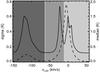 |
Fig. 1 The median 21-cm spectrum (dashed) and the standard-deviation spectrum (solid) of the N1 field; the shaded backgrounds show the LSR velocity ranges used to estimate LVC, IVC and HVC components (from light to dark grey). |
The brightness temperature of each velocity channel was converted to column density, assuming an opacity correction for Hi gas with a constant spin temperature Ts, to provide an estimate of the total Hi column density of each component: 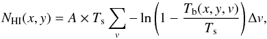 (1)where A = 1.823 × 1018cm-2(Kkms-1)-1. In the optically-thin case (assuming Ts ≫ Tb) this reduces to NHI(x,y) = A ∑ vTb(x,y,v)Δv.
We used Ts = 80K which is compatible with the collisional temperature found from the H2 observations for column densities near 1020cm-2 (Gillmon et al. 2006; Wakker 2006). It is also similar to the average Hi spin temperature (column density weighted) found by Heiles & Troland (2003). Ts will be higher for the WNM, but for these high latitude diffuse lines of sight Tb ≪ 80K for the broad WNM lines, and so adopting the wrong Ts is of no consequence. For most fields the correction is less than 3% compared to the optically-thin assumption. Indeed very few of our 21-cm spectra reach brightness temperatures above 40K – only 3% of the spectra in POL field, the brightest one in the sample. For these “extreme” cases the opacity correction to the column density reaches 35%. Figures 2 and 3 show the Hi column density maps of all fields, in units of 1020cm-2.
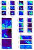 |
Fig. 2 Hi column density maps in units of 1020cm-2 for the AG, DRACO, G86, MC, NEP, SP, N1 and BOOTES fields. To show the full detail, the range is different for each Hi component for a given field. The LSR velocity range used to compute each Hi component map is given in brackets (unit iskms-1). |
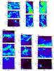 |
Fig. 3 Like Fig. 2 for fields UMAEAST, POLNOR, POL, SPIDER, UMA and SPC. The M81-M82 complex can be seen in the UMA field near l = 142.5°, b = 41.0° in the three Hi components. It was masked in the analysis (see Fig. 13). |
2.3. Uncertainties in NHI
The main analysis presented here relies on a correlation analysis between far-infrared/submm brightness and NHI of the components deduced from 21-cm emission. In order to estimate properly the uncertainties of the deduced correlation coefficients, we need to evaluate the uncertainty of the values of NHI for the Hi components. The method described in Appendix A takes advantage of the fact that the GBT observations were obtained in two polarisations. The difference between these spectra gives a direct estimate of the uncertainty in each channel, which can be integrated over the appropriate velocity ranges, providing a column density uncertainty for each Hi component. The average Hi column densities and uncertainties, expressed in units of 1020cm-2, are given in Table 1 for the three Hi components of each field. This table gives also the average velocity of each Hi component and an estimate of the half-width at half-maximum of the 21-cm feature.
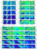 |
Fig. 4 Dust/gas correlation in N1 (top-left), MC (top-right) and BOOTES (bottom): Planck and IRAS raw maps (left column), the model of the dust emission based on the Hi observations (middle: Hi model, |

3. Planck and IRAS
3.1. Map construction
Our analysis uses infrared to submm data at 3000 and 5000GHz (100 and 60μm, respectively) from IRAS (IRIS, Miville-Deschênes & Lagache 2005) and at 353, 545, and 857GHz (850, 550, and 350μm, respectively) from Planck (DR2 release; Planck HFI Core Team 2011b), beginning with maps in Healpix form (Górski et al. 2005) with Nside = 2048 (pixel size of 1.7′). We concentrated here on the three highest frequencies of Planck to avoid the significant contamination from residual CMB fluctuations and interstellar emission other than thermal dust (CO, synchrotron, free-free and spinning dust).
To obtain infrared-submm maps corresponding to each GBT field we first projected each Healpix map, using the nearest neighbour method, onto SFL grids with a pixel size of 1.7′. Each grid was centred on a given GBT field with a size 10% larger in each direction in order to avoid edge effects in subsequent convolution steps. Each SFL map was then converted to MJysr-1 and point sources were removed and replaced by interpolation of the surrounding map2. The map was then convolved to bring it to the GBT 9.4′ resolution and finally projected, using bi-linear interpolation, on the actual GBT grid (3.5′pixel-1). The Planck and IRAS maps for our fields are shown in Figs. 4 to 11. As will be discussed in Sect. 4, these figures also show models of this emission based on Hi observations in a masked subset of the map, and the residual map on subtracting this model from the entire field. The residuals are largest for those areas in the map not used to constrain the model.
3.2. Dust brightness uncertainty
To estimate the noise level of the Planck and IRAS maps we used the method described in Sect. 5.1 of Miville-Deschênes & Lagache (2005). For both data sets we used the difference of maps of the same region of the sky obtained with different sub-samples of the data. These difference maps, properly weighted by their coverage maps, provide an estimate of the statistical properties of the noise. For Planck the noise was estimated using the difference of the first and second half ring maps (Planck HFI Core Team 2011b). In the case of IRAS, each ISSA plate is the combination of up to three maps built from independent observations over the life of the satellite. We built difference maps from these three sets of maps. The procedure used to estimate the Planck and IRAS noise levels at the GBT resolution is detailed in Appendix B. The noise levels for each field and each frequency are given in Table B.1.
4. Dust–HI correlation
4.1. Model
Many studies, mostly using the IRAS and COBE data compared with various 21-cm surveys (Boulanger & Pérault 1988; Joncas et al. 1992; Jones et al. 1995; Boulanger et al. 1996; Arendt et al. 1998; Reach et al. 1998; Lockman & Condon 2005; Miville-Deschênes et al. 2005), have revealed the strong correlation between far-infrared/submm dust emission and 21-cm integrated emission WHI3 at high Galactic latitudes. In particular Boulanger et al. (1996) studied this relation over the whole high Galactic latitude sky. They reported a tight dust–Hi correlation for WHI < 250Kkms-1, corresponding to NHI < 4.6 × 1020cm-2. For higher column densities the dust emission systematically exceeds that expected by extrapolating the correlation. Examining specific high Galactic latitude regions, Arendt et al. (1998) and Reach et al. (1998) found infrared excesses with respect to NHI, with a threshold varying from 1.5 to 5.0 × 1020cm-2.
Part of this excess is due to the effect of 21-cm self-absorption that produces a systematic underestimate of the column density when deduced with the optically thin assumption. Even though this effect is only at a level of a few percent in our case because of the low column densities, applying an opacity correction (see Sect. 2.2) helps to limit this systematic effect.
Most of the infrared/submm excess is usually attributed to dust associated with hydrogen in molecular form. This hypothesis is in accordance with UV absorption measurements that show a sudden increase of the H2 absorption at NH = (3 − 5) × 1020cm-2 (Savage et al. 1977; Gillmon et al. 2006), roughly the threshold for departure from the linear correlation between dust emission and NHI. It is also observed that the pixels showing evidence of excess are spatially correlated and correspond to, or at least are in the vicinity of, known molecular clouds traced by CO emission. See also the discussion in Sect. 6.1.
A third source of this excess emission could be dust associated with the Warm Ionized Medium (WIM) but detection of this component is difficult (Arendt et al. 1998; Lagache et al. 2000) because there is no direct tracer of the ionized gas column density; Hα depends on the square of the electron density and part of the structure seen in Hα might be back-scattering of diffuse Galactic emission on dust and not photons produced within cirrus clouds (Witt et al. 2010).
Finally, in the most diffuse regions of the high-latitude sky, the fluctuations of the CIB are a significant fraction of the brightness fluctuations in the infrared/submm. With a power spectrum flatter (k-1) than that of the interstellar dust emission (k-3) (Miville-Deschênes et al. 2002b, 2007; Lagache et al. 2007; Planck Collaboration 2011n), the CIB anisotropies contribute mostly at small angular scales, producing statistically homogeneous brightness fluctuations over any observed field, like an instrumental noise. Furthermore, because the CIB is unrelated to interstellar emission, the CIB fluctuations cannot be responsible for the excess of infrared emission seen at moderate to high NHI column density.
In the analysis presented here we go a few steps further than the previous studies by: 1) allowing for different dust emissivities for the local ISM (i.e., LVC), IVC, and HVC components; 2) applying an opacity correction to the 21-cm brightness temperatures in order to compute a more reliable NHI; and 3) taking into account explicitly the CIB fluctuations which turn out to dominate the uncertainties in the derived emissivities.
In some fields (like G86 with strong IVC emission) the distinctive morphology of the IVC column density map can be seen clearly in the line-of-sight integrated dust emission map (see Figs. 2 and 5 and Martin et al. 1994), but even faint signals can be brought out by formal correlation analysis. We use the following model: 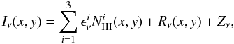 (2)where Iν(x,y) is the dust map at frequency ν (IRAS or Planck),
  the emissivity of Hi component i (LVC, IVC and HVC), and Zν is the zero level of the map. Rν represents not only the contribution from noise in the data but also any emission in the IRAS and Planck bands that is not correlated with NHIincluding the CIB anisotropies and potential dust emission coming from molecular or ionized gas. In this model we assume that the three HI components
  have a constant emissivity over the field. Any spatial variations of the emissivity would also contribute to fluctuations in Rν(x,y).
4.2. Estimating the dust emissivities
To estimate the parameters and constant Zν we used the IDL function regress which, in the case of a general linear least-squares fit, solves the following equation (Press et al. 1995): 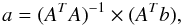 (3)where a is the vector of the parameters and b is a vector of the N IRAS or Planck data points from the map, divided by their respective error:
  (4)A is an N × M matrix that includes the NHI values of the M Hi components,
 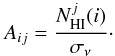 (5)Regress uses a Gaussian elimination method for the inversion.
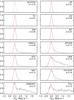 |
Fig. 12 Normalised PDF of the residual R857 of the dust-gas correlation at 857GHz for each field after convergence of the masking procedure. The red curve is the result of a Gaussian fit to the lower, rising part of the PDF. |
For the model described in Eq. (2), the least-squares fit method provides a maximum-likelihood estimation of the parameters provided that the residual term Rν(x,y) is uncorrelated with  and its fluctuations are normally distributed (i.e., white noise). In addition, in order that the parameter estimates not be biased, the uncertainties on have to be comparatively small; we will show (see Sect. 4.5) that this last condition is satisfied for our data. On the other hand, we will also show that the residual term Rν(x,y) is clearly not compatible with white noise. Even for the most diffuse fields in our sample, where the CIB fluctuations dominate the residual emission and the Probability Density Function (PDF) of Rν(x,y) is normally distributed, the condition that there be no (not even chance) correlation with NHI is not satisfied, because the power spectrum of the CIB is not white, but rather like k-1 (Planck Collaboration 2011n). For brighter fields, where spatial variation of the dust emission with respect to the Hi templates is expected (due to the presence of molecules, a poor Hi opacity correction, or spatial variation of dust properties), the residual is not even normally distributed.
To limit the influence of these effects, and in order to focus on estimating the dust emissivity of the Hi components, we relied on a masking procedure to flag and remove obvious outliers with respect to the correlation, and on Monte-Carlo simulations to estimate the uncertainties and bias (see Sect. 4.5).
4.3. Masking
In order to limit the effect of lines of sight with significant “excess” dust emission that is not associated with Hi gas, most previous authors used only data points with NHI lower than a given threshold to stay in a regime of linear correlation. This thresholding was motivated by the fact that above some NHI the extinction and self-shielding of H2 are strong enough to limit photo-dissociation, whereas below the threshold the hydrogen is mostly atomic. The threshold depends sensitively on local gas density and temperature but for typical interstellar conditions for CNM gas (n = 100cm-3, T = 80K, G = 1, where G is the scaling factor of the InterStellar Radiation Field (ISRF) as defined by Mathis et al. (1983)), it is about NHI = 2.5 × 1020cm-2 (Reach et al. 1998). Others have used a quadratic function for ϵν (Fixsen et al. 1998) based on the idea that the H2 column density depends (at least dimensionally) on  (Reach et al. 1994). Both methods introduce a bias in the parameter estimation that is difficult to quantify.
Instead of applying an arbitrary cutoff in NHI, Arendt et al. (1998) used an iterative method to exclude data points above a cut along lines perpendicular to the fit, in order to arrive at a stable solution for ϵν. We used a similar approach by iteratively masking out data points that would produce a positively-skewed residual. That way we expect to keep pixels in the maps that correspond to lines of sight where the dust emission is dominated by the atomic Hi components.
The PDF of residual map, R, defined as 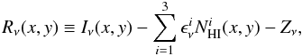 (6)is used to estimate the mask. We used the Planck 857-GHz channel because it has the best signal-to-noise ratio and is less sensitive than the IRAS channels to dust temperature-induced emissivity variations. For the most diffuse fields in our sample (AG, MC, N1, BOOTES, G86, SP) the PDF of R857 is very close to a Gaussian, which suggests that the model described by Eq. (2) is the right one in such low column density regions.
Accordingly, for the first iteration of the masking process for each field, we performed the multi-variate linear regression based on Eqs. (3) to (5) using only the faintest 10% pixels in the 857 GHz map. For further iterations this threshold was relaxed, bringing in more pixels in the map compatible with the iterated model.
As discussed above, the presence of dust emission associated with molecular gas can positively skew the PDF, and empirically the PDF of R857 is indeed positively skewed for the eight remaining fields (Fig. 12). To determine the set of pixels to be retained, we used a Gaussian fit to the lower, rising part of the PDF, up to the PDF maximum, and estimated the σ (see the red curves in Fig. 12). With the above motivation, we assume that the lower part of the PDF is representative of pixels where the fit works well (i.e., for these pixels the residual is normally distributed). Using the σ fit only to this part of the PDF, we apply a threshold in R857 by masking out all pixels with R857 > 3 × σ away from the mean. We iteratively recompute the parameters and mask to converge on a stable solution. The PDFs of R857 obtained at the end of the process are shown in Fig. 12.
Emissivities of each Hi component at 353, 545, 857, 3000, and 5000GHz.
For the six faintest fields, the masking excluded less than 1% of the points. For these fields the mask has no significant effect on the estimated parameters. For the eight other fields, the masking method excluded from 17 to 83% of the pixels. The masks for these eight fields are shown in Fig. 13. In these cases the masking has a significant effect on the result, but we have checked that the estimated parameters are similar to the ones obtained with a NHI ≤ 4 × 1020cm-2 threshold. In fact the masking method used here allows us to keep pixels that would have been excluded by a simple NHI thresholding even though they do not depart significantly from the linear correlation.
Table 2 provides the  values for each field/component/frequency. In order to visualize the results, Fig. 14 gives scatter plots together with the line of slope
  for each component, field by field. Specifically, for each HI component i we plotted
 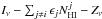 as a function of .
4.4. Statistics of the residual
Figures 4 to 11 show the IRAS and Planck maps, together with the Hi correlated emission and the residual maps Rν for all our fields. For the six faintest fields (N1, SP, BOOTES, AG, MC, and G86 – see Figs. 4–5), the structure in the residuals is, even by visual inspection, clearly spatially correlated between frequencies, especially in the Planck bands. It is dominated by small scale structures with equally negative and positive brightness fluctuations. The structure of the residual for brighter fields is also clearly correlated between frequencies but in these cases the residual is mostly positive (i.e., they are excesses with respect to the Hi). These residuals also show larger coherent structures than in the fainter fields.
The rms (about the mean) of the residual R can be approximated as: 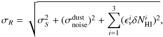 (7)where noise in the IRAS or Planck data and that induced by uncertainties in NHI are explicitly accounted for and σS includes all other contributions not in the model, including CIB anisotropies and dust emission associated with molecular gas. After quadratic subtraction Fig. 15 shows the value of σS at each frequency, as a function of the average NHI density for each field. For fields with a median column density lower than 2 × 1020cm-2, the PDFs of the residual emission all have skewness and kurtosis values compatible with a Gaussian distribution. Furthermore the width of these PDFs shows very small scatter from field to field (see Fig. 15). This is another indication that, for such diffuse fields, the model is a good description of the data; i.e., the Galactic dust emission is largely dominated by the Hi components, with very limited spatial variations of the emissivity across a given field.
The dashed line gives the average level of σS for those fields with NHI < 2 × 1020cm-2. These quantities, together with the average Planck or IRAS and GBT noise contributions to σR, are summarized in Table 3. It is clear from Table 3 and Fig. 15 that even for faint fields σS is the main contributor to the rms of the residual, and therefore the main contributor to the dispersion in the dust-gas correlation diagrams in these fields. This is in accordance with the findings of Planck Collaboration (2011n) who concluded that the CIB fluctuations dominate σS at 353GHz and higher frequencies.
At higher column densities, the PDF of the residual shows positive skewness and an rms that increases with NHI, significantly exceeding the level of CIB anisotropies. These aspects of the PDF indicate one or more extra components that contribute to the dust emission and are not taken into account in our model. Contributions to the residual that grow with NHI are compatible with the presence of a molecular gas component. This could also come from spatial variations of the dust emissivity for given Hi components or from inadequately-separated Hi components.
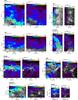 |
Fig. 13 Mask for the eight fields where more than 1% of the pixels were excluded (NEP = 17%, POL = 83%, SPC = 26%, POLNOR = 30%, SPIDER = 24%, UMA = 56%, UMAEAST = 66%, DRACO = 29%). For each field the left image is the total Hi integrated emission and the right image is the Planck 857GHz map. The regions in greyscale were excluded from the correlation analysis. Note the relationship of the masks to the regions of high residual in Figs. 5 to 11. |
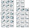 |
Fig. 14 I857 vs. NHI scatter plots, visualising the dust-gas correlation for each of the three Hi components, across a row. The fields POL and POLNOR do not have an HVC component. For a given Hi component, the remaining 857GHz emission, once the contribution of the other two Hi components has been removed, is plotted as a function of NHI of that component (i.e., |
Average of the standard deviations of the sky residual σS for the six fields with ⟨ NHI ⟩ lower than 2 × 1020cm-2 (AG, BOOTES, G86, MC, N1, and SP).
4.5. Monte-Carlo method to determine emissivity uncertainties
The statistical uncertainties estimated for the emissivities by the least-squares fit method are accurate only for the case of white Gaussian noise in Iν and (sufficiently) low noise in the NHI components. The noise in Iν includes IRAS or Planck instrumental noise, CIB anisotropies, and various interstellar contaminants, and for the most diffuse fields in our sample, its PDF is close to Gaussian. However, its power spectrum is certainly not white. First, at the angular scales of our observations (from 9′ to a few degrees), the power spectrum of the CIB anisotropies is P(k) ∝ k-1 (Planck Collaboration 2011n). Second, the spatial variation of the coverage and the convolution to the GBT resolution both introduce spatial structure in the noise that modifies its power spectrum. The addition of all those noise sources produces a net noise term nν on Iν that is not white. Because of the random chance correlation of nν with the NHI components, the uncertainties on the parameters estimated from the least-squares are systematically underestimated (the least-squares fit is not optimal). In addition, the NHI maps are not noise free; significant noise on the independent variable in a least-squares fit produces a systematic bias in the solution. Furthermore, imperfect opacity correction of the Hi spectra, the presence of molecular gas, and spatial variations of the dust properties will also produce non-random fluctuations in the residual map. For all of these reasons, an analysis of Monte-Carlo simulations is required for proper estimation of the uncertainties and biases in the .
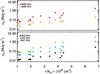 |
Fig. 15 Value of σS obtained from the standard deviation σR of the residual maps Rν(x,y) from which contributions from the IRAS or Planck and the GBT noise were removed quadratically (see Eq. (7)), plotted as a function of the average HI column density of each field (sum of LVC, IVC and HVC). The dashed line is the average of σS for fields with NHI < 2 × 1020cm-2 (see Table 3). |
To generate simulations for each field, we adopted the NHI maps obtained from the 21-cm observations as templates of the dust emission. We built dust maps  for each frequency ν by adding up these NHI maps multiplied by their respective estimated emissivities (just as in computing the residual), to which we added realizations of the IRAS or Planck noise nν appropriate to the field4 at a level compatible with Table 3 once convolved at GBT resolution, and of the sky residual aν with a k-1 power spectrum at a level to reproduce σS within the mask5:
 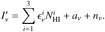 (8)Before fitting these simulated data we added white noise to each NHI component at the level estimated for the GBT data (Table 1). We then carried out the least-squares fit, using the mask already estimated for each field. From a thousand such simulations for each field, we obtained the statistics of the recovered
  so that we could determine if our original fit (fed into the simulation) was biased and could compare the dispersion of the parameters to the statistical uncertainties returned by the least-squares fitting procedure.
Table 4 summarizes the results of the Monte-Carlo simulations. Due to random correlation between nν and the NHI components, we find the Monte-Carlo-derived uncertainty in is several times higher than the analytically-derived uncertainty. The results are reported in the table in terms of φν, the ratio of  , the standard deviation of the emissivities recovered in the simulations, to
  , the standard deviation expected from the linear fit performed by Regress. Therefore, in what follows we use the values of as the uncertainties in (see Table 2).
Finally, these simulations make it possible for us to estimate any bias in which could arise from the noise in NHI. Table 4 also provides the bias in %: 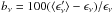 . Except for some (undetected) HVCs, the bias is only at the few percent level; in what follows we made no correction for it.
Results from the Monte-Carlo simulations.
5. Results
5.1. Planck and IRAS emissivities
The present study extends to smaller scales, and to the IVCs and HVCs, the earlier work done with the FIRAS (Boulanger et al. 1996) or IRAS (Boulanger & Pérault 1988; Reach et al. 1998) data on the dust emission of the diffuse ISM. It also extends to a much larger sample a similar analysis done on a diffuse 3° × 3° region at high Galactic latitude using IRAS and Spitzer data (Miville-Deschênes et al. 2005). The IR/submm-Hi correlation analysis allows us to determine empirically the spectral dependence of the ratio between the dust emission and the gas column density. In addition, the combination of Planck, IRAS, and NHI data can be used to trace one elusive component of the diffuse interstellar medium: the diffuse H2 gas (Sect. 6.1).
As seen in Fig. 14 there is a clear correlation between the IRAS or Planck data and NHI in all fields but, as previously seen with COBE and IRAS data, there are increasing excesses of dust emission with increasing NHI. The estimated emissivities for each field/component/frequency are compiled in Table 2 and shown in Fig. 16. We note that dust associated with the LVC and IVC components is detected in each field and at each frequency, unlike for HVCs for which we do not report any significant detection. All HVC emissivities are indeed below 3σ. The results on HVCs are discussed further in Sect. 6.3. In the following we analyse what can be drawn from the emissivities for the LVCs and IVCs.
 |
Fig. 16 SEDs from the emissivities of LVC (black) and IVC (blue) components for all the fields in our sample. For each Hi component in each cloud, the solid line is the modified black body fit using 353, 545, 857, and 3000GHz data. |
5.2. Comparison with FIRAS data
The FIRAS data provide a reference for the dust emission spectrum of the diffuse ISM. The average FIRAS SED of the high-Galactic latitude sky used by Compiègne et al. (2011) to set the diffuse ISM dust properties in the DustEM model is shown in Fig. 17. Also shown in this figure are the current results (red symbols) for the average of the emissivities for the LVCs of our sample at 353, 545, 857, 3000, and 5000GHz. The IRAS and Planck data points are found to be fully compatible with the diffuse ISM FIRAS spectrum, showing that our sample is representative of the diffuse dust emission at high Galactic latitudes. We have fit model parameters to both data sets independently using a modified black body function:  (9)where Bν(T) is the Planck function, mH the mass of hydrogen, μ the mean molecular weight and κ0 is the opacity of the dust–gas mixture at some fiducial frequency ν0. The higher-frequency (60μm) IRAS datum is not used in the fit due to contamination by non-equilibrium emission from stochastically-heated smaller grains (Compiègne et al. 2011). The top panel of Fig. 17 shows the data divided by the model to better display the quality of the fit. The values found for T and β with the two data sets are in close accord. This analysis shows that the local ISM SED can be fit well with T = 17.9K and β = 1.8.
5.3. The spectral energy distribution
Figure 16 shows the dust SED for each field and Hi component separately, with the error bars computed using the Monte-Carlo simulations. We first note that all the LVC and IVC SEDs are at a similar level showing that the power emitted per H is comparable between fields. Second, in many cases, the SED of IVCs peaks at a higher frequency than for the LVCs. That could be caused by a higher temperature or a larger abundance of smaller grains in the IVCs.
Like for the FIRAS comparison, each SED was fit using a modified black body function (solid lines). It has been shown by several studies (Dupac et al. 2003; Désert et al. 2008; Shetty et al. 2009; Veneziani et al. 2010) how difficult it is to estimate separately T and β for such an SED fit. These two parameters are significantly degenerate; their estimate depends greatly on the accuracy of the determination of the error bars on the SED data points and on the correlation of the errors between frequencies. The estimate of T and β also depends on the spectral range used to make the fit; for a typical T = 18K dust emission spectrum, the Rayleigh-Jeans range of the black body curve, where β can be well estimated, corresponds to ν < 375GHz (λ > 800μm).
Because of the above caveats relating to simultaneous fits of T and β, and because the FIRAS spectrum of the diffuse ISM is compatible with β = 1.8 (in this case the large number of data points and the broad frequency coverage over the peak of the SED give more confidence in the value of β obtained), we have carried out SED fitting assuming a fixed β = 1.8. This provides a direct way to compare not only with the FIRAS spectrum and the DustEM model, but also with similar analyses with Planck data on molecular clouds and in the Galactic plane (Planck Collaboration 2011o,q,u) that used the same convention.
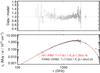 |
Fig. 17 Bottom panel: black points show the FIRAS spectrum of the diffuse ISM (Compiègne et al. 2011). The red points are the average of the IRAS or Planck emissivities for the local components of all our fields; the uncertainty is the variance of the values divided by |

5.4. Dust properties
The modified black-body fit (Eq. (9)) provides information on the properties, such as T, of the dust in each Hi component. A useful quantity used below is the emission cross-section of the interstellar material per H: 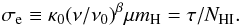 (10)It is simply the prefactor to the Planck function in Eq. (9). In what follows we adopt ν0 = 1200GHz (λ0 = 250μm) to compare directly with the value of σe(1200) = τ/NHI at 250μm given by Boulanger et al. (1996).
A key quantity is the luminosity per H atom L (in W/H) emitted by dust grains (equal to the absorbed power) computed by integrating the SED over ν: 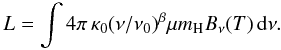 (11)Complementing the actual SEDs in Fig. 16, Fig. 18 shows the derived values of σe(1200), T and L plotted against the velocity of each Hi component (LVC and IVC) in our sample.
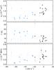 |
Fig. 18 Values of σe at 1200GHz (250μm), T and L versus the average velocity of each Hi component. These dust parameters were estimated from the SED fit over the range 353 to 3000GHz to a modified black body with β = 1.8. Black and blue symbols are for LVC and IVC, respectively. The different symbols in blue represent IVCs associated with specific complexes: IV Arch (dot), IV/LLIV Arch (triangle), Complex K (square) and PP Arch (star). In each panel the dotted line represent the value for the diffuse ISM obtained with the high-latitude FIRAS spectrum (see Fig. 17). Error bars are given for each data point, some being smaller than the symbol size. |
The average emission cross-section for the 14 LVC components of our sample is 1.0 ± 0.3 × 10⁻²⁵cm2, in good agreement with the value of 1 × 10-25cm2 obtained by Boulanger et al. (1996). The scatter of σe(1200) for the LVCs (30%) is not the result of errors.
The emission cross-section for the IVC components is different, often 50% lower compared to the LVCs. There appear to be differences among the IVCs too, perhaps related to the fact that they belong to different IVC complexes. All fields in our sample overlap with the Intermediate Velocity (IV) Arch, except MC which is in the southern Galactic sky and belongs to the PP Arch and BOOTES which is part of Complex K (Kuntz & Danly 1996). The North Celestial Loop also overlaps spatially with the Low-Latitude Intermediate Velocity (LLIV) Arch (Kuntz & Danly 1996), an Hi feature at slightly less negative velocity (~−50 kms-1) than the IV Arch (~−75 kms-1). The fields UMA and UMAEAST contain clumps identified by Kuntz & Danly (1996) as being part of the LLIV Arch (specifically LLIV1, LLIV2 and LLIV3). The field POL also contains emission that can be attributed to the LLIV Arch. These different complexes are identified with separate symbols in Fig. 18. The outliers are POL, UMAEAST (high) and MC (low). Excluding these σe = 0.5 ± 0.2 × 10⁻²⁵cm2 for the rest.
The values of T for the LVCs (T = 17.9 ± 0.9K) are in accordance with that obtained from the FIRAS spectrum at high Galactic latitude (T = 17.9 ± 0.1K; Fig. 17) and also close to the 17.5K found by Boulanger et al. (1996) assuming β = 2. Like for σe, a systematic difference in T is found between LVCs and IVCs, even though it is less statistically significant. On average the IVC group of clouds6 has T = 20.0 ± 1.0K, a value greater than in the local ISM at the 2.1σ level. Note the different IVC complexes as well.
Regarding L the striking result here is the small variation observed over all the fields and Hi components. Combined together, the LVCs and IVCs have ⟨ L ⟩ = 3.4 ± 0.6 × 10⁻³¹W/H, representing a variation of only 20% over all clouds. The fact that L is rather constant over all fields and Hi components can also be appreciated in Fig. 16, where all SEDs are at about the same level. The small variation of L is surprising as it indicates that the power absorbed by dust is also rather constant, possibly suggesting constancy of the radiation field across all fields even at the distance of IVCs.
We have made the same analysis with a floating β to evaluate the robustness of the results shown in Fig. 18. The greatest impact of a floating β is on the uncertainty of T, and to a lesser degree on σe. The values of L are particularly insensitive because the modified black-body still serves effectively as an interpolation function between the measured data points. Even though the uncertainties on T and σe increase with a floating β, the trends seen in Fig. 18 are still observed, even more pronounced. We conclude that using β = 1.8 is a reasonable and conservative approach.
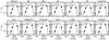 |
Fig. 19 Correlation coefficient of the residual emission with the 857GHz residual. Similar to Fig. 16, the solid line here is the normalised modified black body SED fit using 3000, 545 and 353GHz data. We assumed a fixed β = 1.8, except for the six most diffuse fields (MC, G86, AG, N1, SP and BOOTES) where the residual emission is dominated by the CIB fluctuations. In these fields β = 1.8, typical of diffuse Galactic dust emission, does not provide a good fit; these SEDs require a smaller value of β (see text). |
5.5. SED of the residual emission
As seen in Figs. 4 to 11, the residual emission once the Hi model is subtracted from the Planck and IRAS maps exhibits significant spatial coherence which reproduces from frequency to frequency. In order to estimate the SED of this residual emission in each field, we carried out a linear regression analysis between the residual map at each frequency and the residual map at 857GHz. The resulting slope of the regression (in units of MJysr-1/MJysr-1 and equal to 1 at 857GHz, by construction) can be used to estimate the shape of the spectrum of this residual emission. The results are presented in Fig. 19.
As for the SEDs of the Hi-correlated emission, the SEDs of the residual are well fit by a modified black body function. We note a significant difference in the SED shape between low Hi column density fields and brighter regions. The SEDs of brighter fields, where the residual emission is likely to come from molecular gas (Sect. 6.1), could be fit with β = 1.8 but with a slightly lower temperature (T = 16.1 ± 0.6K) than the LVC components. On the other hand, the SED of fainter fields, where the residual emission is most probably dominated by CIB anisotropies, could not be fit with β = 1.8. It is better described with T = 18.6 ± 0.9 and β = 1.1 ± 0.1. This should be taken only as a convenient fitting function, nothing physical. The significantly different value of β found here is probably the result of the complex composite nature of these fluctuations coming from the combination of all galaxies along the line of sight in slices of redshift which change with frequency (Planck Collaboration 2011n).
6. Discussion
6.1. The Hi-H2 transition
One possible contribution to the residual emission is dust associated with ionized gas. The WIM has a vertical column density of about 1 × 1020cm-2 (Reynolds 1989; Gaensler et al. 2008), a significant fraction of the total column density in the most diffuse areas of the sky. Planck Collaboration (2011n) showed that, once the emission correlated with Hi is removed from the Planck 353, 545 and 857GHz data in faint fields, the residual emission has a power spectrum compatible with k-1, much flatter than any interstellar emissions. We also showed that the amplitude of the residual in faint fields is constant from field to field (see Fig. 15), compatible with an isotropic extra-galactic emission. These are strong indications that dust emission associated with the WIM, and not correlated with Hi, is small.
In the eight fields with bright cirrus, the residuals to the IR-Hi correlation are skewed toward positive values, larger than the amplitude of the CIB fluctuations. The most straightforward interpretation is that these positive residuals trace dust emission within H2 gas. This interpretation is reinforced by the fact that in the brightest fields (e.g., UMA, UMAEAST, and POL) we have checked that the residual emission is very well correlated with CO emission (Dame et al. 2001; Planck Collaboration 2011o), confirming the previous study of Reach et al. (1998) in the North Celestial Loop region (see their Fig. 11). The lower dust temperature estimated from the SED of the residual emission in all these bright fields (see Fig. 19) is also reminiscent of what is observed in molecular clouds (Planck Collaboration 2011u).
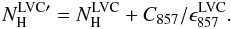
In the following we assume that the submm excess emission provides a way to estimate the molecular gas column density within the local ISM (LVC) component7. In order to estimate the fraction of H2 in our fields we carried out an analysis using the I857 dust maps and the following equation explained below:  (12)To concentrate on the local (LVC) gas, we removed the IVC and HVC-correlated emission and the constant term from I857, using the above results of the linear regression in each field. Assuming the dust emissivity is the same in the molecular gas as in the atomic gas from which it formed, we divided this by
  for each field to produce estimated maps of the total column density
  for the local/low-velocity gas. We note that this map still includes the fluctuations of the CIB (C857) that act like a noise on the true total column density
  :
:  (13)We of course have a map of the LVC atomic column density (
 ) from the GBT measurements. Therefore, we are able to compute an estimate of the molecular column density map
 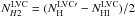 and then calculate an estimate of the fraction of mass (or fraction of H nuclei) in molecular form,
  , pixel by pixel. The results obtained by combining all pixels in all fields, except DRACO, are plotted in Fig. 20. To produce this figure we binned the data in and within each bin examined the PDF of f(H2), finding its median (dark symbol) and half-power points (error bars, which are not necessarily symmetrical).
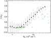 |
Fig. 20 Fraction f(H2) of hydrogen that is in molecular form in local gas/LVC, calculated from emission excess relative to the linear correlation (see text), versus the total column density estimated using the 857GHz dust emission transformed into gas column density using the emissivities ϵν. Black points show the median value of f(H2) in bins of NH computed using all lines of sight in our sample. The error bars show the half-width at half maximum of the PDF computed in each NH bin. Green symbols show the results obtained using UV absorption data from high-latitude surveys (Gillmon et al. 2006; Wakker 2006, squares) and toward O stars on lines of sight closer to the Galactic Plane (Rachford et al. 2002, 2009, triangles). |
On this figure are also plotted estimates of f(H2) using FUSE data by Gillmon et al. (2006); Wakker (2006) (squares – high-latitude lines of sight) and Rachford et al. (2009) (triangles – Galactic Plane lines of sight). The combination of these two datasets covers the column density range probed in our analysis.
The results plotted in Fig. 20 reveal an increase in f(H2) beginning at  cm-2 and reaching 0.8 for NH ~ 4 × 1021cm-2. Note that we are not sensitive to the much lower values of f(H2) found by FUSE at low column densities. For pixels with
  cm-2 the dispersion of our estimate of f(H2) is due to the fluctuations of the CIB. For these pixels,
  and therefore
 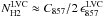 . Because C857 has a mean of zero, it produces both positive and negative values of f(H2).
Note that the UV observations toward O stars in the Galactic Plane (triangles) give some f(H2) values at the same level as we find, but also some much lower values for a given column density. This suggests that the UV observations are somewhat affected by clumpiness and/or are sampling qualitatively different lines of sight than ours at high latitude. Indeed Wakker (2006) emphasized that it is not straightforward to relate the Hi-H2 transition to physical properties of the interstellar gas, like density in the molecule-producing environment, or even a physical threshold in column density required for molecule formation, because of the summing over different environments along the line of sight. A corollary is that there can be quite different values of f(H2) for the same NH, as is seen in the figure, and so comparison of UV data with the complementary infrared/submm analysis is of great interest.
The overall correspondance between the trends seen independently in the Planck and FUSE results supports our interpretation of the submm excess being caused by dust associated with molecular hydrogen. We would call this medium “dark gas” if it were not detected via CO (Planck Collaboration 2011o). Although there are lines of sight where f(H2) is quite high, summed over all lines of sight in our survey, our study shows that the excess emission at 857GHz that is not correlated with Hi is only 10% of the total emission. Thus the fraction of the hydrogen gas mass that is in molecular form in this sample of the high latitude diffuse interstellar medium in the solar neighbourhood is quite low. Planck Collaboration (2011o) estimated a value of 35% for the entire high-latitude sky above 15°, which includes higher column density lines of sight (this introduces yet another factor, Hi self-absorption, to make the medium dark). Of this 35%, about half is traced by CO, leaving about 20% as “dark gas” not traced by CO or Hi.
The structure and nature of the diffuse molecular gas can be studied using the maps of residual (excess) dust emission. In SPIDER (see Fig. 9), an intermediate column density field where there is very little CO emission detected (Barriault et al. 2010), we observe coherent filamentary structures in the residual map that we interpret as the presence of dust in diffuse H2 gas without CO. We have checked that the structures cannot be accounted for by an underestimate of the 21-cm line opacity correction, being present even with Tspin as low as 40K. In this field the submm residual provides a way to map the first steps of the formation of molecules in the diffuse ISM.
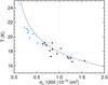 |
Fig. 21 Temperature vs emission cross-section at 1200GHz (250μm) estimated from modified black-body fit with β = 1.8 to data from 353 to 3000GHz. Black is for LVCs, blue IVCs: IV Arch (dot), IV/LLIV Arch (triangle), Complex K (square) and PP Arch (star). The solid line respresents a constant emitted luminosity L corresponding to the diffuse ISM reference values (σe = 1 × 10-25cm-2 and T = 17.9K – dotted lines). |
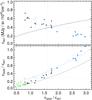 |
Fig. 22 Top: dust emission per NHI at 857GHz versus the 3000/857 GHz (100/350μm) ratio. Local (black), IVC (blue – dot is IV Arch, triangle IV/LLIV Arch, square Complex K), residual (green). Solid line is the DustEM model for the diffuse ISM (Compiègne et al. 2011), with radiation field variations from G = 0.1 to G = 5. Dashed line is the same model but with a relative abundance of VSGs four times higher than the standard diffuse ISM value. Dotted lines gives the local ISM fiducial values (G = 1.0). Typical uncertainties are shown for each Hi component. Bottom: 5000/857 GHz (60/350μm) ratio as a function of the 3000/857 GHz (100/350μm) ratio. |
6.2. Evolution of dust
6.2.1. Variations of the big grain emission cross-section
Interstellar dust evolves through grain-grain and gas-grain interactions. Fragmentation and coagulation of dust grains are expected to occur in the ISM, modifying not only the grain size distribution but also the grain structure. The data described here provide important evidence for dust processing in diffuse local clouds and IVCs. As we will elucidate, the evidence foreshadowed in Fig. 18 can be seen in Figs. 21 and 22.
Figure 21 shows the values of T and σe(1200) already shown in Fig. 18 but here as a scatter plot. The solid line shows the expected σe(1200) as a function of T for a constant emitted luminosity L (normalized to 3.8 × 10⁻³¹W/H, the average diffuse ISM values for T = 17.9K and σe(1200) = 1.0 × 10⁻²⁵cm-2).
The emission cross-section σe reflects the efficiency of thermal dust emission per unit mass. Dust that emits more efficiently will have a lower equilibrium temperature, the trend seen. Note that the dust in very different environments has close to the same integrated emission (L) and therefore is absorbing about the same power (solid line). The comparison with the values found in the Taurus molecular cloud by Planck Collaboration (2011u) (T ~ 14.5K, β = 1.8, σe ~ 2.0 × 10⁻²⁵cm-2 and L = 2.3 × 10⁻³¹W/H) suggests that the T − σe anti-correlation extends to colder dust and denser environments, although the typical power absorbed is lower because of shielding.
Because σe depends only on the dust properties and on the dust-to-gas ratio, the 30% variation observed in local ISM (LVC – see Fig. 18), where we expect little variations of the metallicity, is interpreted as a genuine variation of the dust properties from one cloud to another. An alternative explanation would be the presence of different amounts of H2 gas spatially correlated with the Hi. In this case the dust opacity σe(1200) would be overestimated due to an underestimate of the actual gas column density. Although this scenario cannot be excluded formally, the data shown here does not support an increase of σe(1200) with NHI through the Hi-H2 transition, as one might expect in this case. For this reason we favor an interpretation of the variations of σe(1200) related to modifications of the grain properties.
Figure 22 complements Fig. 21 by comparing directly measured emissivities (ϵν) with the DustEM model of the average diffuse high latitude emission. This comparison, independent of any modified black-body fit, also shows strong evidence for dust evolution. The top plot of Fig. 22 shows the 857GHz emissivity versus the 3000GHz to 857GHz ratio. This is compared to a simple DustEM model prediction for constant dust properties and a variation of the radiation field strength from G = 0.1 to G = 5 (G = 1 being the fiducial value). The prediction of DustEM is an increase of both ϵ857 and ϵ3000/ϵ857 with increasing radiation field strength, and therefore T. The former increases with G simply because of the increase of Bν(T). The ratio ϵ3000/ϵ857 increases with T as the peak of the black-body shifts towards higher frequencies. The data points do not follow this trend showing clearly that the variations in the SEDs found here in LVCs and IVCs cannot be explained by local variations of the radiation field strength. The data are consistent with a decrease of the dust emission cross-section (~ϵ857) with temperature (~ϵ3000/ϵ857), the same trend seen in Fig. 21. An evolutionary model in which dust structure changes due to aggregation (and the reverse process, fragmentation) is qualitatively consistent with these results: grains with a fluffy structure will absorb about the same amount of optical and ultraviolet radiation per unit mass as more compact grains, but compared to these more homogeneous and spherical grains they are more emissive at submm wavelengths because of their more complex structure and therefore cool more efficiently (Stepnik et al. 2003).
Upper limit for the HVC emissivities in each field.
6.2.2. Dust shattering in Intermediate Velocity clouds?
The bottom plot of Fig. 22 shows the 5000GHz to 857GHz emissivity ratio as a function of the 3000GHz to 857GHz ratio for all Hi components and the residual emission SEDs. The locus from standard ISM DustEM models shows an effect of increasing colours with increasing G. The bright cirrus clouds of the LVC components (black symbols at the left end of the plot) and the molecular residuals (green) have colours in good agreement with the standard DustEM model, consistent with some variation of G ≲ 1.
Both ratios are higher for the IVCs and the trend is offset relative to the standard locus. The qualitative interpretation is that the emission in these higher-frequency bands is more contaminated by non-equilibrium emission from an increased relative abundance of very small grains (VSGs) compared to the larger grains (BGs) in thermal equilibrium. To make this more quantitative, the dashed curve passing closer to the IVC data shows the colours for a DustEM diffuse ISM model with a relative abundance of VSGs four times higher than the standard value.
Because of their non-equilibrium emission, VSGs dominate the emission for ν > 5000GHz and, according to the standard DustEM model and for the standard radiation field (G = 1), contribute to 30% of the emission in the IRAS 60μm band even with an abundance of only 1.6% of the total dust mass. By contrast, the BGs make up 90.7% of the total dust mass, 14.2% carbon rich and 76.5% silicates. Therefore an increase of a factor four of the mass in VSGs is easy to accommodate by shattering of a small fraction of the BG dust mass. The fact that the emission cross-section of IVCs is a factor of two lower than for the local ISM can be due to a decrease of the mass in BGs (i.e., the dust-to-gas mass ratio) and/or to a decrease in the emission cross-section of a single grain, the latter affecting the equilibrium dust temperature. For the average temperature found in IVCb (T = 20.4 K), and considering a variation of the dust-to-gas mass ratio from 1 to 1/2 the local ISM value, the radiation field strength needed to explain these results would be G = 1 − 2, not an unreasonable range for IVCs. It is thus difficult to conclude at this point on the exact nature of the variation of σe in IVCs. On the other hand these results are clearly compatible with a modification of the BGs (total mass and/or grain properties) and a significant increase of the abundance of VSGs. The details would be linked to the specific dynamical and shock history of this interstellar matter that is part of the Galactic fountain (Shapiro & Field 1976; Houck & Bregman 1990).
6.3. Dust in high-velocity clouds
Dust emission in HVCs is expected to be weak for several reasons. First, their great distance from the Galactic disk (typically several kpc – Wakker 2001; van Woerden & Wakker 2004) implies a faint radiation field, hence a low dust equilibrium temperature and a low luminosity (Wakker & Boulanger 1986; Trifalenkov 1993; Miville-Deschênes et al. 2005). But the main reason comes from gas phase abundance measurements obtained from absorption lines of oxygen, silicon and iron in the far-UV. Because oxygen is mostly in the gas phase and because its ionization potential is similar to hydrogen, the ratio Oi/Hi provides the most robust measure of metallicity in diffuse clouds. Unlike oxygen, iron and silicon are depleted into dust grains in the local ISM (Savage & Sembach 1996); low ratios of Si/O and Fe/O thus trace the presence of dust. In most HVCs the Oi/Hi ratio shows that the metallicity is significantly sub-solar (of the order 0.1–0.5 solar, see Lu et al. 1998; Wakker et al. 1999; Richter et al. 2001; Tripp et al. 2003; Sembach et al. 2004; van Woerden & Wakker 2004; Fox et al. 2006; Collins et al. 2007), indicative of their extragalactic origin. In addition the Si/O and Fe/O ratios in Complex C are infered to be close to solar (Richter et al. 2001; Collins et al. 2007) indicating little silicon and iron locked in dust grains. Together the overall low abundance of metals and the fact that Si and Fe seem to be mostly in the gas phase imply a low dust to gas ratio in HVCs.
Nevertheless, because of the unknown enrichment history of HVCs that might set different intrinsic abundances than in the solar sytem8, the difficulty to estimate the effect of ionization on Siii and Feii to infer the abundances of Si and Fe9, and the unkown nature of dust in HVCs10, the link between the metallicity, the depletions and the amount of dust remains indicative. One illustrative related example, albeit for an IVC, is the finding by Richter et al. (2001) of only mild depletion of Si and Fe for the IVC IV-Arch which nevertheless has dust emission at a comparable level to the local ISM. Thus the search for dust emission from HVCs is an interesting complementary way to put contraints on the physical conditions and nature of matter in the Galactic halo.
After unsuccesful attemps to detect dust emission from HVCs using IRAS data (Wakker & Boulanger 1986; Fong et al. 1987; Bates et al. 1988; Désert et al. 1988), Miville-Deschênes et al. (2005) claimed a detection in Complex C using a combination of Spitzer, IRAS and GBT data. Compared to these previous searches, the analysis presented here extend greatly the number of fields, the surface covered and the wavelength coverage. The fields used here overlap with four HVC complexes: Complex C (DRACO, G86, N1, NEP, SP, SPIDER, BOOTES11), Complex M (AG), Complex A (SPC, UMA, UMAEAST) and the Magellanic Stream (MC). HVC-correlated emission is not detected significantly in any of these fields.
At each frequency the emissivities found are compatible with zero within 3σ, with about as many negative as positive values. At first glance, examination of the emissivities in Table 2 shows systematic behaviour across frequencies that could be taken as encouraging evidence for an HVC detection in some fields, like AG. However, this does not necessarily bolster the statistical significance of the detection in a single pass band. This is because the dust emission is intrinsically highly correlated frequency to frequency, as is the CIB, and so given the generally small noise, the fits to the correlations with (the same) NHI are to first order just scaled versions of each other. This analysis establishes the main difficulties hampering the detection of dust emission from HVCs, the contaminating foreground emission of LVCs and IVCs and the background CIB fluctuations which greatly increase the uncertainties in  (Sect. 4.5 and Table 4).
In Table 5 we focus on the upper limits to the HVC emissivities. They were computed using a Bayesian approach in the case of Gaussian errors with a bounded physical region (Feldman & Cousins 1998); we assumed that the true emissivities can only be zero or positive. Table 5 gives the value of ϵν for which there is 99.87% probability (equivalent to a 3σ upper limit) that the true emissivity is ≤ ϵν. These upper limits are compared in Table 5 to the weighted average of the measured emissivites for the LVC and IVC components; any dust in HVCs has an emissivity, on average, no more than 15% of the value found in the local ISM at 857 and 3000GHz.
We considered the null hypothesis that the HVC emissivity is zero (or a small uniform value) in all fields and find that, at any given frequency, the weighted standard deviation of the measured HVC emissivities (σ(ϵ)) is somewhat larger than expected given the uncertainties on each measurement. This is true even when considering only AG, N1, MC and SP, the fields with significant HVC Hi column density and almost no masking. For example, the probability of obtaining the measured σ(ϵ) is only 0.2% at 857GHz for these four fields. One explanation could be that we have underestimated the uncertainties on each measurement; to increase the probability of the measured σ(ϵ) to 10% at 857GHz, the uncertainties would need to be multiplied by 1.6. But even such a moderate increase of the uncertainties seems unlikely in the most diffuse fields considered here because the noise is dominated by the strongly constrained and well modeled CIB fluctuations (Planck Collaboration 2011n). A second explanation is that the σ(ϵ) reflects a variation of the true ϵ from field to field. For these four fields we verified that, if one allows for a variation of ϵ from field to field following a uniform distribution in the range between zero and the upper limit of each field, the probability of obtaining the measured σ(ϵ) reaches 15% at 857GHz without having to increase the uncertainties on the individual measurements. If this is the right explanation, the measured value of σ(ϵ) implies that ϵ is small but non-zero in some fields.
Finally, there have been many interesting discussions of the possible relationships between IVCs and HVCs (e.g., Albert & Danly 2004; Wakker 2001). Here the relative emissivity is of some relevance; as our data show, Hi-correlated emission is readily detected in IVCs, but not in HVCs. A specific example is provided by our AG field which encompasses the cloud MI in HVC Complex M (Wakker 2001). The low HVC emissivity in contrast to the fairly normal IVC emissivity (Table 2) does not support any direct relationship between MI and the intermediate velocity gas in the IV Arch in this direction (Wakker 2001).
7. Conclusions
We have presented results of a first comparison of Planck and IRAS with new Hi 21-cm line GBT data for 14 high Galactic latitudes fields, covering about 825deg2 on the sky. Using the velocity information of the 21-cm data we made column density maps of the LVC, IVC, and HVC in each field. By correlating these Hi maps with the submm/infrared dust emission maps we estimated the distinct dust emissivities for these three high-latitude components and made corresponding SEDs from 353 to 5000GHz.
On average, the dust SED of the local ISM (LVC) deduced from the IRAS and Planck data is compatible with that from the FIRAS data over the high-latitude sky and is well fit with a modified black body with parameters β = 1.8 and T = 17.9K. On the other hand, even though the energy emitted by dust is rather constant in our sample, we report significant variations of the dust SED shape, compatible with variations of the dust temperature anti-correlated with the emission cross-section. We interpret these variations as a signature of active evolution of the dust grain structure through coagulation and fragmentation in the diffuse ISM.
For faint cirrus fields with average Hi column density lower than 2 × 1020cm-2, the residual FIR-submm emission, after removal of the Hi-correlated contributions, is normally distributed with a standard deviation compatible with the expected level of CIB fluctuations. The SED of the residual is unlike any interstellar component. For such diffuse fields we also show that the interstellar dust emission is dominated by the contribution from atomic gas.
For fields with larger Hi column density there are significant FIR-submm emission excesses that, for the brightest fields, follow the structure of the CO emission. For intermediate column density regions, the residual emission shows coherent spatial structures not seen in CO, revealing the presence of H2 gas. The SED of this residual shows that it is slightly colder than the dust in the local Hi. There is a lot of variation in f(H2), the fractional mass in the form of H2, but over the whole survey of these diffuse fields the fraction is only 10%.
We report strong detection of dust emission from all IVCs in our sample. The dust emission cross-section is typically two times lower than for the local ISM and the relative abundance of small grains having non-equilibrium emission is about four times higher than normal. This evolution of the dust properties is indicative of dust shattering in halo gas with the dynamics of a Galactic fountain. We also find that, compared to the local ISM, several of these clouds have a higher dust temperature which could also be the result of globally smaller grains. The total energy emitted by dust in IVCs is comparable to what is observed in the local ISM suggesting similar radiation field strength.
Finally, we have attempted to detect HVC-correlated dust emission. We show why this is very challenging, because of the uncertainties induced by foreground contamination and the CIB anisotropies. The average of the 99.9% confidence upper limits on the emissivity, 0.15 times the average emissivity found in the local ISM at 857 and 3000GHz, is compatible with the low level of dust emission expected from HVCs based on their low metallicity and relatively low depletion of elements like Si and Fe.
Planck (http://www.esa.int/Planck) is a project of the European Space Agency (ESA) with instruments provided by two scientific consortia funded by ESA member states (in particular the lead countries France and Italy), with contributions from NASA (USA) and telescope reflectors provided by a collaboration between ESA and a scientific consortium led and funded by Denmark.
For Planck channels we removed only point sources identified in the ERCSC (Planck Collaboration 2011c). For IRAS maps we used the source removal method described in Miville-Deschênes & Lagache (2005).
Equivalent to optically-thin Hi column density.
We assumed white noise maps for both IRAS and Planck, each divided by the square root of their coverage map.
For the faintest fields this will produce a map with the statistical properties of the CIB anisotropies. For brighter fields, where the residual also includes interstellar contributions, we assumed it also follows a k-1 power spectrum, but with a greater normalisation (i.e., σS) to take into account these effects.
Excluding POL, UMAEAST and MC.
This is not true for the DRACO field where the excess emission is likely to be dominated by Intermediate-Velocity gas which has accompanying CO emission (Herbstmeier et al. 1993). For this reason this field was discarded in the current analysis.
O and Si are mostly produced in Type II supernovae, Fe is produced primarly in Type Ia supernovae.
The true abundance of Si and Fe are less than the ones infered from Siii/Hi and Feii/Hi. To take this bias into account, an ionization correction is applied (Collins et al. 2003) that depends on gas density and radiation field strength, both not well constrained.
The amount of carbonaceous dust is not constrained by gas phase abundances.
BOOTES is on the side of Complex C. It has faint emission from –80 to –100kms-1 that could also be associated with the IVC Complex K.
Acknowledgments
A description of the Planck Collaboration and a list of its members can be found at http://www.rssd.esa.int/index.php?project=PLANCK&page=Planck_Collaboration. We thank the anonymous referee for many helpful comments.
References
- Albert, C. E., & Danly, L. 2004, in High Velocity Clouds, ed. H. van Woerden, B. P. Wakker, U. J. Schwarz, & K. S. de Boer, 312, 73 [Google Scholar]
- Arendt, R. G., Odegard, N., Weiland, J. L., et al. 1998, ApJ, 508, 74 [Google Scholar]
- Barriault, L., Joncas, G., Falgarone, E., et al. 2010, MNRAS, 406, 2713 [NASA ADS] [CrossRef] [Google Scholar]
- Bates, B., Catney, M. G., & Keenan, F. P. 1988, Ap&SS, 146, 195 [NASA ADS] [CrossRef] [Google Scholar]
- Bersanelli, M., Mandolesi, N., Butler, R. C., et al. 2010, A&A, 520, A4 [NASA ADS] [CrossRef] [EDP Sciences] [Google Scholar]
- Blagrave, K., Lockman, F. J., & Martin, P. G. 2010, in The Dynamic Interstellar Medium: A Celebration of the Canadian Galactic Plane Survey, ed. A. G. W. R. Kothes, & T. L. Landecker, ASP Conf. Ser., 438, 156 [Google Scholar]
- Boothroyd, A., Blagrave, K., Lockman, F., Martin, P., et al. 2011, A&A, in press, DOI: 10.1051/0004-6361/201117656 [Google Scholar]
- Boulanger, F., & Pérault, M. 1988, ApJ, 330, 964 [NASA ADS] [CrossRef] [Google Scholar]
- Boulanger, F., Abergel, A., Bernard, J., et al. 1996, A&A, 312, 256 [NASA ADS] [Google Scholar]
- Calabretta, M. R., & Greisen, E. W. 2002, A&A, 395, 1077 [NASA ADS] [CrossRef] [EDP Sciences] [Google Scholar]
- Collins, J. A., Shull, J. M., & Giroux, M. L. 2003, ApJ, 585, 336 [NASA ADS] [CrossRef] [Google Scholar]
- Collins, J. A., Shull, J. M., & Giroux, M. L. 2007, ApJ, 657, 271 [NASA ADS] [CrossRef] [Google Scholar]
- Compiègne, M., Verstraete, L., Jones, A., et al. 2011, A&A, 525, A103 [NASA ADS] [CrossRef] [EDP Sciences] [Google Scholar]
- Dame, T. M., Hartmann, D., & Thaddeus, P. 2001, ApJ, 547, 792 [NASA ADS] [CrossRef] [Google Scholar]
- Désert, F., Macías-Pérez, J. F., Mayet, F., et al. 2008, A&A, 481, 411 [NASA ADS] [CrossRef] [EDP Sciences] [Google Scholar]
- Désert, F. X., Bazell, D., & Boulanger, F. 1988, ApJ, 334, 815 [NASA ADS] [CrossRef] [Google Scholar]
- Dupac, X., Bernard, J., Boudet, N., et al. 2003, A&A, 404, L11 [NASA ADS] [CrossRef] [EDP Sciences] [Google Scholar]
- Feldman, G. J., & Cousins, R. D. 1998, Phys. Rev. D, 57, 3873 [Google Scholar]
- Field, G. B. 1965, ApJ, 142, 531 [NASA ADS] [CrossRef] [Google Scholar]
- Field, G. B., Goldsmith, D. W., & Habing, H. J. 1969, ApJ, 155, L149 [NASA ADS] [CrossRef] [Google Scholar]
- Fixsen, D. J., Dwek, E., Mather, J. C., Bennett, C. L., & Shafer, R. A. 1998, ApJ, 508, 123 [NASA ADS] [CrossRef] [Google Scholar]
- Fong, R., Jones, L. R., Shanks, T., Stevenson, P. R. F., & Strong, A. W. 1987, MNRAS, 224, 1059 [NASA ADS] [CrossRef] [Google Scholar]
- Fox, A. J., Savage, B. D., & Wakker, B. P. 2006, ApJS, 165, 229 [NASA ADS] [CrossRef] [Google Scholar]
- Gaensler, B. M., Madsen, G. J., Chatterjee, S., & Mao, S. A. 2008, PASA, 25, 184 [NASA ADS] [CrossRef] [Google Scholar]
- Gillmon, K., Shull, J. M., Tumlinson, J., & Danforth, C. 2006, ApJ, 636, 891 [NASA ADS] [CrossRef] [Google Scholar]
- Górski, K. M., Hivon, E., Banday, A. J., et al. 2005, ApJ, 622, 759 [NASA ADS] [CrossRef] [Google Scholar]
- Heiles, C., & Troland, T. H. 2003, ApJ, 586, 1067 [NASA ADS] [CrossRef] [Google Scholar]
- Herbstmeier, U., Heithausen, A., & Mebold, U. 1993, A&A, 272, 514 [NASA ADS] [Google Scholar]
- Houck, J. C., & Bregman, J. N. 1990, ApJ, 352, 506 [NASA ADS] [CrossRef] [Google Scholar]
- Ingalls, J. G., Miville-Deschênes, M., Reach, W. T., et al. 2004, ApJS, 154, 281 [NASA ADS] [CrossRef] [Google Scholar]
- Joncas, G., Boulanger, F., & Dewdney, P. E. 1992, ApJ, 397, 165 [NASA ADS] [CrossRef] [Google Scholar]
- Jones, M. H., Rowan-Robinson, M., Branduardi-Raymont, G., et al. 1995, MNRAS, 277, 1587 [NASA ADS] [Google Scholar]
- Kuntz, K. D., & Danly, L. 1996, ApJ, 457, 703 [NASA ADS] [CrossRef] [Google Scholar]
- Lagache, G., Haffner, L. M., Reynolds, R. J., & Tufte, S. L. 2000, A&A, 354, 247 [Google Scholar]
- Lagache, G., Bavouzet, N., Fernandez-Conde, N., et al. 2007, ApJ, 665, L89 [NASA ADS] [CrossRef] [Google Scholar]
- Lamarre, J., Puget, J., Ade, P. A. R., et al. 2010, A&A, 520, A9 [NASA ADS] [CrossRef] [EDP Sciences] [Google Scholar]
- Lockman, F. J., & Condon, J. J. 2005, AJ, 129, 1968 [NASA ADS] [CrossRef] [Google Scholar]
- Low, F. J., Young, E., Beintema, D. A., et al. 1984, ApJ, 278, L19 [NASA ADS] [CrossRef] [Google Scholar]
- Lu, L., Sargent, W. L. W., Savage, B. D., et al. 1998, AJ, 115, 162 [NASA ADS] [CrossRef] [Google Scholar]
- Mandolesi, N., Bersanelli, M., Butler, R. C., et al. 2010, A&A, 520, A3 [Google Scholar]
- Martin, P. G., Rogers, C., Reach, W. T., Dewdney, P. E., & Heiles, C. E. 1994, in The First Symposium on the Infrared Cirrus and Diffuse Interstellar Clouds, ed. R. M. C. W. B. Latter, ASP Conf. Ser., 58, 188 [Google Scholar]
- Martin, P. G., Miville-Deschênes, M., Roy, A., et al. 2010, A&A, 518, L105 [NASA ADS] [CrossRef] [EDP Sciences] [Google Scholar]
- Mathis, J. S., Mezger, P. G., & Panagia, N. 1983, A&A, 128, 212 [NASA ADS] [Google Scholar]
- Mennella, A., Butler, R. C., Curto, A., et al. 2011, A&A, 536, A3 [NASA ADS] [CrossRef] [EDP Sciences] [Google Scholar]
- Miville-Deschênes, M., & Lagache, G. 2005, ApJS, 157, 302 [NASA ADS] [CrossRef] [Google Scholar]
- Miville-Deschênes, M., Boulanger, F., Joncas, G., & Falgarone, E. 2002a, A&A, 381, 209 [NASA ADS] [CrossRef] [EDP Sciences] [Google Scholar]
- Miville-Deschênes, M., Lagache, G., & Puget, J. 2002b, A&A, 393, 749 [NASA ADS] [CrossRef] [EDP Sciences] [Google Scholar]
- Miville-Deschênes, M., Boulanger, F., Reach, W. T., & Noriega-Crespo, A. 2005, ApJ, 631, L57 [NASA ADS] [CrossRef] [Google Scholar]
- Miville-Deschênes, M., Lagache, G., Boulanger, F., & Puget, J. 2007, A&A, 469, 595 [NASA ADS] [CrossRef] [EDP Sciences] [Google Scholar]
- Miville-Deschênes, M., Martin, P. G., Abergel, A., et al. 2010, A&A, 518, L104 [NASA ADS] [CrossRef] [EDP Sciences] [Google Scholar]
- Planck Collaboration 2011a, A&A, 536, A1 [NASA ADS] [CrossRef] [EDP Sciences] [Google Scholar]
- Planck Collaboration 2011b, A&A, 536, A2 [NASA ADS] [CrossRef] [EDP Sciences] [Google Scholar]
- Planck Collaboration 2011c, A&A, 536, A7 [NASA ADS] [CrossRef] [EDP Sciences] [Google Scholar]
- Planck Collaboration 2011d, A&A, 536, A8 [NASA ADS] [CrossRef] [EDP Sciences] [Google Scholar]
- Planck Collaboration 2011e, A&A, 536, A9 [NASA ADS] [CrossRef] [EDP Sciences] [Google Scholar]
- Planck Collaboration 2011f, A&A, 536, A10 [NASA ADS] [CrossRef] [EDP Sciences] [Google Scholar]
- Planck Collaboration 2011g, A&A, 536, A11 [NASA ADS] [CrossRef] [EDP Sciences] [Google Scholar]
- Planck Collaboration 2011h, A&A, 536, A12 [NASA ADS] [CrossRef] [EDP Sciences] [Google Scholar]
- Planck Collaboration 2011i, A&A, 536, A13 [NASA ADS] [CrossRef] [EDP Sciences] [Google Scholar]
- Planck Collaboration 2011j, A&A, 536, A14 [NASA ADS] [CrossRef] [EDP Sciences] [Google Scholar]
- Planck Collaboration 2011k, A&A, 536, A15 [NASA ADS] [CrossRef] [EDP Sciences] [Google Scholar]
- Planck Collaboration 2011l, A&A, 536, A16 [NASA ADS] [CrossRef] [EDP Sciences] [Google Scholar]
- Planck Collaboration 2011m, A&A, 536, A17 [NASA ADS] [CrossRef] [EDP Sciences] [Google Scholar]
- Planck Collaboration 2011n, A&A, 536, A18 [NASA ADS] [CrossRef] [EDP Sciences] [Google Scholar]
- Planck Collaboration 2011o, A&A, 536, A19 [NASA ADS] [CrossRef] [EDP Sciences] [Google Scholar]
- Planck Collaboration 2011p, A&A, 536, A20 [NASA ADS] [CrossRef] [EDP Sciences] [Google Scholar]
- Planck Collaboration 2011q, A&A, 536, A21 [NASA ADS] [CrossRef] [EDP Sciences] [Google Scholar]
- Planck Collaboration 2011r, A&A, 536, A22 [NASA ADS] [CrossRef] [EDP Sciences] [Google Scholar]
- Planck Collaboration 2011s, A&A, 536, A23 [NASA ADS] [CrossRef] [EDP Sciences] [Google Scholar]
- Planck Collaboration 2011t, A&A, 536, A24 [Google Scholar]
- Planck Collaboration 2011u, A&A, 536, A25 [NASA ADS] [CrossRef] [EDP Sciences] [Google Scholar]
- Planck Collaboration 2011v, The Explanatory Supplement to the Planck Early Release Compact Source Catalogue (ESA) [Google Scholar]
- Planck Collaboration 2011w, A&A, 536, A26 [NASA ADS] [CrossRef] [EDP Sciences] [Google Scholar]
- Planck HFI Core Team 2011a, A&A, 536, A4 [NASA ADS] [CrossRef] [EDP Sciences] [Google Scholar]
- Planck HFI Core Team 2011b, A&A, 536, A6 [NASA ADS] [CrossRef] [EDP Sciences] [Google Scholar]
- Press, W. H., Teukolsky, S. A., Vetterling, W. T., & Flannery, B. P. 1995, Numerical Recipes in C (Cambridge University Press), 994 [Google Scholar]
- Rachford, B. L., Snow, T. P., Tumlinson, J., et al. 2002, ApJ, 577, 221 [NASA ADS] [CrossRef] [Google Scholar]
- Rachford, B. L., Snow, T. P., Destree, J. D., et al. 2009, ApJS, 180, 125 [NASA ADS] [CrossRef] [Google Scholar]
- Reach, W. T., Koo, B., & Heiles, C. 1994, ApJ, 429, 672 [NASA ADS] [CrossRef] [Google Scholar]
- Reach, W. T., Wall, W. F., & Odegard, N. 1998, ApJ, 507, 507 [NASA ADS] [CrossRef] [Google Scholar]
- Reynolds, R. J. 1989, ApJ, 339, L29 [NASA ADS] [CrossRef] [Google Scholar]
- Richter, P., Sembach, K. R., Wakker, B. P., et al. 2001, ApJ, 559, 318 [NASA ADS] [CrossRef] [Google Scholar]
- Savage, B. D., & Sembach, K. R. 1996, ARA&A, 34, 279 [NASA ADS] [CrossRef] [Google Scholar]
- Savage, B. D., Bohlin, R. C., Drake, J. F., & Budich, W. 1977, ApJ, 216, 291 [NASA ADS] [CrossRef] [Google Scholar]
- Sembach, K. R., Wakker, B. P., Tripp, T. M., et al. 2004, ApJS, 150, 387 [NASA ADS] [CrossRef] [Google Scholar]
- Shapiro, P. R., & Field, G. B. 1976, ApJ, 205, 762 [NASA ADS] [CrossRef] [Google Scholar]
- Shetty, R., Kauffmann, J., Schnee, S., Goodman, A. A., & Ercolano, B. 2009, ApJ, 696, 2234 [NASA ADS] [CrossRef] [Google Scholar]
- Spitzer, Jr., L. 1956, ApJ, 124, 20 [NASA ADS] [CrossRef] [Google Scholar]
- Stepnik, B., Abergel, A., Bernard, J., et al. 2003, A&A, 398, 551 [NASA ADS] [CrossRef] [EDP Sciences] [Google Scholar]
- Tauber, J. A., Mandolesi, N., Puget, J., et al. 2010, A&A, 520, A1 [NASA ADS] [CrossRef] [EDP Sciences] [Google Scholar]
- Trifalenkov, I. A. 1993, Astron. Rep., 37, 327 [NASA ADS] [Google Scholar]
- Tripp, T. M., Wakker, B. P., Jenkins, E. B., et al. 2003, AJ, 125, 3122 [NASA ADS] [CrossRef] [Google Scholar]
- van Woerden, H., & Wakker, B. P. 2004, in High Velocity Clouds, ed. H. van Woerden, B. P. Wakker, U. J. Schwarz, & K. S. de Boer, 312, 195 [Google Scholar]
- Veneziani, M., Ade, P. A. R., Bock, J. J., et al. 2010, ApJ, 713, 959 [NASA ADS] [CrossRef] [Google Scholar]
- Wakker, B. P. 2001, ApJS, 136, 463 [NASA ADS] [CrossRef] [Google Scholar]
- Wakker, B. P. 2006, ApJS, 163, 282 [NASA ADS] [CrossRef] [Google Scholar]
- Wakker, B. P., & Boulanger, F. 1986, A&A, 170, 84 [NASA ADS] [Google Scholar]
- Wakker, B. P., Howk, J. C., Savage, B. D., et al. 1999, Nature, 402, 388 [NASA ADS] [CrossRef] [PubMed] [Google Scholar]
- Wheelock, S., Gautier, T. N., Chillemi, J., et al. 1993, ISSA Explanatory Suppl., Tech. Rep. [Google Scholar]
- Witt, A. N., Gold, B., Barnes, F. S., et al. 2010, ApJ, 724, 1551 [NASA ADS] [CrossRef] [Google Scholar]
- Zacchei, A., Maino, D., Baccigalupi, C., et al. 2011, A&A, 536, A5 [NASA ADS] [CrossRef] [EDP Sciences] [Google Scholar]
Appendix A: Noise of the Hi components
The analysis presented here relies on a correlation between far-infrared/submm data and the Hi components deduced from 21-cm emission. In order to estimate properly the uncertainties on the correlation coefficients the noise on the Hi components needs to be evaluated. We have made this estimate using two different methods which address different contributions to the noise (see Boothroyd et al. 2011).
First we applied the traditional method in which the end channels of the 21-cm spectrum, where there is no emission. The velocity channels are independent, i.e., the spectrometer resolution is better than the 0.8kms-1 channel width. A large number of end channels can be used to compute a map of the standard deviation of the noise at each (x,y) position: 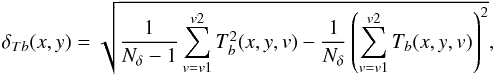 (A.1)where Nδ = v2 − v1 + 1 is of the order of 200 channels. For the GBT data, this is a very flat map, whose typical value is the same as the standard deviation of a single end channel. This is about 0.17K for a single visit to a field. Some fields were mapped two or three times.
The uncertainty map δNHI(x,y) for the column density of a given Hi component summed over N channels is ![Mathematical equation: \appendix \setcounter{section}{1} \begin{equation} \delta N_{\rm HI}(x,y) ~ [\mbox{cm}^{-2}] = A \sqrt{N} \delta_{Tb}(x,y) \Delta v, \end{equation}](/articles/aa/full_html/2011/12/aa16485-11/aa16485-11-eq949.png) (A.2)where Δv is the channel width in kms-1. For N ~ 60, this amounts to δNHI ~ 0.02 × 1020cm-2 for a single visit. This assumes, as is usual, that the noise properties estimated using the end channels are representative of the noise in channels summed to build the column density maps. Actually, the channel noise scales as roughly (1 + Tb/20K) and this can be taken into account.
(A.2)where Δv is the channel width in kms-1. For N ~ 60, this amounts to δNHI ~ 0.02 × 1020cm-2 for a single visit. This assumes, as is usual, that the noise properties estimated using the end channels are representative of the noise in channels summed to build the column density maps. Actually, the channel noise scales as roughly (1 + Tb/20K) and this can be taken into account.
We developed a second method which exploits the fact that the Hi brightness-temperature cubes were built by averaging independent data taken in different polarisations (called XX and YY). Each polarisation observation can be reduced separately, which requires separate baseline estimates for the spectra in the XX and YY cubes. Baseline fitting is another source of error. Taking the difference between the XX and YY cubes removes the common unpolarized Hiemission, leaving in each velocity channel only the thermal noise and systematic effects from the baseline subtraction. The difference cube is  (A.3)where we divide by two to give the same statistics as in the average of the cubes.
We make a map of the column density differences (divided by two) over the same channel range as for NHI: 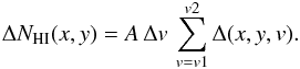 (A.4)The estimate of δNHI is then the standard deviation of this map.
This method gives an uncertainty typically 1.3 times the simple estimate using end channels (it can reach up to 2 times for the brightest components) because it includes baseline uncertainties and the increase of thermal noise with signal. The column density uncertainties evaluated with this second method for each component in each field are given in Table 1). There are additional errors from the stray radiation correction that can affect the local and IVC components. The total uncertainty including this additional contribution can be estimated in a similar way to the second method if there are two or more visits to compare (Boothroyd et al. 2011). Because in cases with multiple visits these are found to be not much larger, and because the uncertainties in NHI are not the major source of uncertainty in the correlation analysis (Sect. 4.5), adopting the values in Table 1 is satisfactory for our purposes.
Appendix B: Estimating the noise of the Planck and IRAS maps
Planck and IRAS noise levels (in MJysr-1) for each field and at each frequency.
To estimate the noise level of the IRAS and Planck maps we use the difference between independent observations of the same sky. For IRAS, the original ISSA plates (Wheelock et al. 1993) were delivered with three independent set of observations (called HCONs), each obtained at different periods during the life of the satellite. Each HCON has its own coverage map. The ISSA final product is the coverage-weighted co-addition of the three HCONs. The IRIS product (Miville-Deschênes & Lagache 2005) also contains the three HCONs.
A similar approach was used to estimate the noise of each Planck map. For each pointing period Planck scans the sky about 50 times. The Data Processing Centre delivered two maps made with data from the first half and second half of each pointing period, respectively. In this case the number of samples used to estimate the signal at a given sky position is the same in the two maps (i.e., the coverage map is identical for the two maps). Again we used the difference between these two maps of the same region of the sky to estimate the noise.
Here we want to estimate the average noise level δIν of an IRAS or Planck map Iν used for the analysis given a difference map  (B.1)obtained from independent observations, each Iν,i map having its own coverage map Nν,i. In the general case (Miville-Deschênes & Lagache 2005), δIν is obtained by taking the standard deviation of the map
 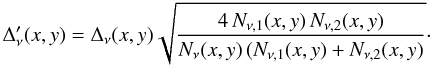 (B.2)In the case of Planck, Nν,1 = Nν,2 = Nν/2 and so
  and the standard deviation of the average map is the same for the difference map, as expected. Because the ISSA plates are the combination of three observations with different coverages such a simplification is not possible and the above more general equation has to be used.
In our analysis we used the IRAS and Planck maps convolved to the 9.4′ resolution of the GBT. Therefore, the appropriate δIν is obtained by first convolving the  map and then taking the standard deviation. These are the noise levels tabulated for each field in Table B.1.
All Tables
Average of the standard deviations of the sky residual σS for the six fields with ⟨ NHI ⟩ lower than 2 × 1020cm-2 (AG, BOOTES, G86, MC, N1, and SP).
Planck and IRAS noise levels (in MJysr-1) for each field and at each frequency.
All Figures
|
Fig. 1 The median 21-cm spectrum (dashed) and the standard-deviation spectrum (solid) of the N1 field; the shaded backgrounds show the LSR velocity ranges used to estimate LVC, IVC and HVC components (from light to dark grey). |
| In the text | |
|
Fig. 2 Hi column density maps in units of 1020cm-2 for the AG, DRACO, G86, MC, NEP, SP, N1 and BOOTES fields. To show the full detail, the range is different for each Hi component for a given field. The LSR velocity range used to compute each Hi component map is given in brackets (unit iskms-1). |
| In the text | |
|
Fig. 3 Like Fig. 2 for fields UMAEAST, POLNOR, POL, SPIDER, UMA and SPC. The M81-M82 complex can be seen in the UMA field near l = 142.5°, b = 41.0° in the three Hi components. It was masked in the analysis (see Fig. 13). |
| In the text | |
|
Fig. 4 Dust/gas correlation in N1 (top-left), MC (top-right) and BOOTES (bottom): Planck and IRAS raw maps (left column), the model of the dust emission based on the Hi observations (middle: Hi model, |
| In the text | |
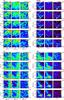 |
Fig. 5 Like Fig. 4, for AG (top-left), DRACO (top-right), SP (bottom-left) and G86 (bottom-right). |
| In the text | |
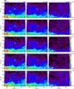 |
Fig. 6 Like Fig. 4, for field SPC. |
| In the text | |
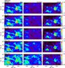 |
Fig. 7 Like Fig. 4, for field UMAEAST. |
| In the text | |
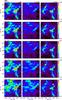 |
Fig. 8 Like Fig. 4, for field UMA. |
| In the text | |
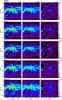 |
Fig. 9 Like Fig. 4, for field SPIDER. |
| In the text | |
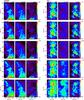 |
Fig. 10 Like Fig. 4, for fields POLNOR (left) and POL (right). |
| In the text | |
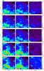 |
Fig. 11 Like Fig. 4, for field NEP, the largest. |
| In the text | |
|
Fig. 12 Normalised PDF of the residual R857 of the dust-gas correlation at 857GHz for each field after convergence of the masking procedure. The red curve is the result of a Gaussian fit to the lower, rising part of the PDF. |
| In the text | |
|
Fig. 13 Mask for the eight fields where more than 1% of the pixels were excluded (NEP = 17%, POL = 83%, SPC = 26%, POLNOR = 30%, SPIDER = 24%, UMA = 56%, UMAEAST = 66%, DRACO = 29%). For each field the left image is the total Hi integrated emission and the right image is the Planck 857GHz map. The regions in greyscale were excluded from the correlation analysis. Note the relationship of the masks to the regions of high residual in Figs. 5 to 11. |
| In the text | |
|
Fig. 14 I857 vs. NHI scatter plots, visualising the dust-gas correlation for each of the three Hi components, across a row. The fields POL and POLNOR do not have an HVC component. For a given Hi component, the remaining 857GHz emission, once the contribution of the other two Hi components has been removed, is plotted as a function of NHI of that component (i.e., |
| In the text | |
|
Fig. 15 Value of σS obtained from the standard deviation σR of the residual maps Rν(x,y) from which contributions from the IRAS or Planck and the GBT noise were removed quadratically (see Eq. (7)), plotted as a function of the average HI column density of each field (sum of LVC, IVC and HVC). The dashed line is the average of σS for fields with NHI < 2 × 1020cm-2 (see Table 3). |
| In the text | |
|
Fig. 16 SEDs from the emissivities of LVC (black) and IVC (blue) components for all the fields in our sample. For each Hi component in each cloud, the solid line is the modified black body fit using 353, 545, 857, and 3000GHz data. |
| In the text | |
|
Fig. 17 Bottom panel: black points show the FIRAS spectrum of the diffuse ISM (Compiègne et al. 2011). The red points are the average of the IRAS or Planck emissivities for the local components of all our fields; the uncertainty is the variance of the values divided by |
| In the text | |
|
Fig. 18 Values of σe at 1200GHz (250μm), T and L versus the average velocity of each Hi component. These dust parameters were estimated from the SED fit over the range 353 to 3000GHz to a modified black body with β = 1.8. Black and blue symbols are for LVC and IVC, respectively. The different symbols in blue represent IVCs associated with specific complexes: IV Arch (dot), IV/LLIV Arch (triangle), Complex K (square) and PP Arch (star). In each panel the dotted line represent the value for the diffuse ISM obtained with the high-latitude FIRAS spectrum (see Fig. 17). Error bars are given for each data point, some being smaller than the symbol size. |
| In the text | |
|
Fig. 19 Correlation coefficient of the residual emission with the 857GHz residual. Similar to Fig. 16, the solid line here is the normalised modified black body SED fit using 3000, 545 and 353GHz data. We assumed a fixed β = 1.8, except for the six most diffuse fields (MC, G86, AG, N1, SP and BOOTES) where the residual emission is dominated by the CIB fluctuations. In these fields β = 1.8, typical of diffuse Galactic dust emission, does not provide a good fit; these SEDs require a smaller value of β (see text). |
| In the text | |
|
Fig. 20 Fraction f(H2) of hydrogen that is in molecular form in local gas/LVC, calculated from emission excess relative to the linear correlation (see text), versus the total column density estimated using the 857GHz dust emission transformed into gas column density using the emissivities ϵν. Black points show the median value of f(H2) in bins of NH computed using all lines of sight in our sample. The error bars show the half-width at half maximum of the PDF computed in each NH bin. Green symbols show the results obtained using UV absorption data from high-latitude surveys (Gillmon et al. 2006; Wakker 2006, squares) and toward O stars on lines of sight closer to the Galactic Plane (Rachford et al. 2002, 2009, triangles). |
| In the text | |
|
Fig. 21 Temperature vs emission cross-section at 1200GHz (250μm) estimated from modified black-body fit with β = 1.8 to data from 353 to 3000GHz. Black is for LVCs, blue IVCs: IV Arch (dot), IV/LLIV Arch (triangle), Complex K (square) and PP Arch (star). The solid line respresents a constant emitted luminosity L corresponding to the diffuse ISM reference values (σe = 1 × 10-25cm-2 and T = 17.9K – dotted lines). |
| In the text | |
|
Fig. 22 Top: dust emission per NHI at 857GHz versus the 3000/857 GHz (100/350μm) ratio. Local (black), IVC (blue – dot is IV Arch, triangle IV/LLIV Arch, square Complex K), residual (green). Solid line is the DustEM model for the diffuse ISM (Compiègne et al. 2011), with radiation field variations from G = 0.1 to G = 5. Dashed line is the same model but with a relative abundance of VSGs four times higher than the standard diffuse ISM value. Dotted lines gives the local ISM fiducial values (G = 1.0). Typical uncertainties are shown for each Hi component. Bottom: 5000/857 GHz (60/350μm) ratio as a function of the 3000/857 GHz (100/350μm) ratio. |
| In the text | |
Current usage metrics show cumulative count of Article Views (full-text article views including HTML views, PDF and ePub downloads, according to the available data) and Abstracts Views on Vision4Press platform.
Data correspond to usage on the plateform after 2015. The current usage metrics is available 48-96 hours after online publication and is updated daily on week days.
Initial download of the metrics may take a while.