| Issue |
A&A
Volume 531, July 2011
|
|
|---|---|---|
| Article Number | A169 | |
| Number of page(s) | 18 | |
| Section | Cosmology (including clusters of galaxies) | |
| DOI | https://doi.org/10.1051/0004-6361/201116851 | |
| Published online | 08 July 2011 | |
Probing the dark-matter halos of cluster galaxies with weak lensing
1
Argelander-Institut für Astronomie, Universität Bonn, Auf dem Hügel 71, 53121 Bonn, Germany
e-mail: emilio@astro.uni-bonn.de
2
Max-Planck-Institut für Astrophysik, Karl-Schwarzschild-Straße 1, 85741 Garching, Germany
Received: 8 March 2011
Accepted: 18 May 2011
Context. Understanding the evolution of the dark matter halos of galaxies after they become part of a cluster is essential for understanding the evolution of these satellite galaxies.
Aims. We investigate the potential of galaxy-galaxy lensing to map the halo density profiles of galaxies in clusters.
Methods. We propose a method that separates the weak-lensing signal of the dark-matter halos of galaxies in clusters from the weak-lensing signal of the cluster’s main halo. Using toy cluster models as well as ray-tracing through N-body simulations of structure formation along with semi-analytic galaxy formation models, we test the method and assess its performance.
Results. We show that with the proposed method, one can recover the density profiles of the cluster galaxy halos in the range 30–300 kpc. Using the method, we find that the weak-lensing signal of cluster member galaxies in the Millennium Simulation is well described by a Navarro-Frenk-White (NFW) profile. In contrast, non-singular isothermal mass distribution (like PIEMD) models provide a poor fit. Furthermore, we do not find evidence for a sharp truncation of the galaxy halos in the range probed by our method. Instead, there is an observed overall decrease of the halo mass profile of cluster member galaxies with increasing time spent in the cluster. This trend, as well as the presence or absence of a truncation radius, should be detectable in future weak-lensing surveys like the Dark Energy Survey (DES) or the Large Synoptic Survey Telescope (LSST) survey. Such surveys should also allow one to infer the mass-luminosity relation of cluster galaxies with our method over two decades in mass.
Conclusions. It is possible to recover in a non-parametric way the mass profile of satellite galaxies and their dark matter halos in future surveys, using our proposed weak lensing method.
Key words: gravitational lensing: weak / galaxies: clusters: general / galaxies: evolution / dark matter
© ESO, 2011
1. Introduction
Astronomical observations indicate that the majority of matter in the Universe is of a yet unknown form that neither emits nor absorbs light (e.g. Komatsu et al. 2011; Percival et al. 2010; Riess et al. 2009). A unique way to study this so-called dark matter and its relation to luminous matter is provided by gravitational lensing (Schneider et al. 2006). Gravitational lensing has been used to probe the matter associated with galaxies (e.g. SLACS survey1, Hoekstra et al. 2004; Mandelbaum et al. 2006; Parker et al. 2007; Mandelbaum et al. 2008; Simon et al. 2008; Tian et al. 2009), clusters (e.g. Clowe et al. 2006; Bradač et al. 2006; Halkola et al. 2006; Halkola et al. 2008; Jee et al. 2009; Schirmer et al. 2010) and the large-scale structure (e.g. Schrabback et al. 2010; Fu et al. 2008; Benjamin et al. 2007).
According to the hierarchical structure formation paradigm, local overdensities created in the early Universe collapse into smaller dark matter halos, in which galaxies form. Larger halos, corresponding to galaxy clusters, form later through accretion and mergers. As a result, a typical galaxy cluster has a massive main halo of dark matter with a bright central galaxy (BCG) at its center. Within this main halo, there are many smaller subhalos hosting a satellite galaxy. These were once isolated objects that merged with the cluster.
An important open question is how subhalos evolve after they become part of a cluster. This is also essential to understand the evolution of the satellite galaxies embedded in them. Simple analytic models assume that subhalos are just stripped of their mass outside some tidal radius by gravitational tidal forces. On the other hand numerical simulations indicate that tidal forces also heat the subhalos causing them to expand and decrease their central density (e.g. Ghigna et al. 1998; Ghigna et al. 2000; Hayashi et al. 2003). In this picture, both tidal stripping and heating continually change the radial mass profiles of subhalos, eventually destroying them.
Most observational studies of subhalos in clusters with gravitational lensing employ parametric models for the mass distribution of the subhalos. Using parametric models has the advantage that one can obtain useful constraints on the model parameters even with a modest amount and quality of lensing data. The method analyzes individual clusters and obtains the mass model parameters as a function of the luminosity of the satellite galaxy (e.g. Limousin et al. 2007; Natarajan et al. 2007; Halkola et al. 2007; Suyu & Halkola 2010). However, a major disadvantage of this approach is that it relies on strong assumptions about the mass profiles of subhalos.
Direct measurements of the mean tangential shear profile around suitably chosen samples of massive objects provide a more direct and less biased view of their mean mass profiles. This approach has been successfully applied to study the halos of field galaxies (e.g. Mandelbaum et al. 2008), and cluster main halos (e.g. Sheldon et al. 2009; Okabe et al. 2010; Israel et al. 2010). However, this approach has a drawback when used for cluster member galaxies and their embedding subhalos: the resulting shear signal probes the subhalo profiles only very close to their center, while the signal becomes dominated at larger distances by the surrounding much more massive cluster main halo.
This problem has been previously considered and studied by Yang et al. (2006). In this work, we propose a modification of the standard weak galaxy-galaxy lensing approach that addresses the latter problem. The key idea is to “calibrate out” the cluster main halo signal by subtracting from the signal measured around the satellite galaxies the tangential shear signal around a specific set of calibration points. As shown in this paper, the additional calibration allows one to reliably probe the subhalo profiles to much larger radii than with the standard galaxy-galaxy lensing approach.
We test the proposed method and assess its performance compared to the standard approach using simulated lensing fields generated from the Millennium Run (Springel et al. 2005). Furthermore, we analyze the resulting subhalos profile as predicted by our simulations and provide forecasts for the signal-to-noise level expected for large upcoming and future surveys like the Dark Energy Survey2 (DES), or the Large Synoptic Survey Telescope3 (LSST) survey. Moreover, we discuss how weak lensing can be used to study the mass loss of subhalos during their evolution in galaxy clusters.
Our paper is organized as follows: in Sect. 2, we briefly discuss the theoretical background. In Sect. 3 we describe our proposed method in detail. A short overview of our simulations is given in Sect. 4. In Sect. 5 we test the performance of our method, we apply it to characterize the dark matter profiles of subhalos in the Millennium simulation, and we forecast signals and noise for upcoming surveys. In Sect. 6 we discuss the most relevant systematic effects for this work. The paper concludes with a summary in Sect. 7.
2. Theory
In this section, we briefly discuss the theory of gravitational lensing needed for our work. We refer the reader to the standard literature (e.g. Bartelmann & Schneider 2001; Schneider et al. 2006) for a detailed discussion.
2.1. Weak lensing basics
A massive foreground structure, the lens, deflects the light emitted by a distant galaxy in its background, the source, toward an observer. Sources at angular position β = (β1,β2) are seen by the observer at a possibly different image position θ = (θ1,θ2). Differential deflection causes distortions in the images of the background galaxies. Locally, the distortion is quantified by the Jacobian  (1)of the lens mapping θ → β. This Jacobian defines the convergence,
  (2)
(2)
the complex shear γ = γ1 + iγ2 where: 
and the reduced shear g = γ/(1 − κ).
Defining a complex ellipticity ϵ = ϵ1 + iϵ2 (Bartelmann & Schneider 2001) for the background sources, the differential light deflection, and thus the mass associated with the lens, can be inferred (statistically) from the measured shape. The relation between the intrinsic ellipticity ϵi and the observed one ϵ are related by:  (4)In the following, we assume the validity of the weak lensing approximation i.e.:
  (5)Note, however, that we test this assumption in Sect. 6.1. Under this approximation and assuming that the ϵi of the different sources are uncorrelated:
  (6)
(6)
2.2. Galaxy-galaxy lensing
In galaxy-galaxy lensing, one measures the tangential ellipticity of a background galaxy image with respect to the position of a foreground lens galaxy,  (7)where φ is the polar angle of the line connecting lens and background image. From Eq. (6) follows that ⟨ϵt⟩ = γt in the weak-lensing regime, where γt denotes the tangential component of the shear with respect to the lens position.
Under the geometrically-thin lens approximation, we can define the excess surface mass density ΔΣ(ξ) at projected physical radius ξ by:  (8)where
  denotes the average surface mass density within a circle of radius ξ, and Σ(ξ) is the average surface mass density on that circle.
The tangential shear γt(ξ) averaged on a circle with physical projected radius ξ around a lens galaxy is related to the excess surface mass density ΔΣ(ξ) by Schneider (2006):  (9)where the critical surface mass density Σcrit is a function of the angular diameter distance to the lens Dd, to the source Ds, and the distance between lens and source Dds:
  (10)An important aspect of galaxy-galaxy lensing is to combine the different measurements from different foreground-background galaxy pairs to increase the signal-to-noise. Each lens-background galaxy pair i with projected separation ξ at the lens, tangential ellipticity ϵt,i of the background galaxy image, and critical surface mass density Σcrit,i provides an estimate
  (11)for the excess surface mass density ΔΣ(ξ) of the lens. For a sample of lens and background galaxies, one can compute the final estimate
  by a weighted mean:
  (12)where the sum runs over all pairs formed by a background image and a lens galaxy. If one assumes that each lens galaxy has the same mass profile and each shear estimate from a background galaxy image carries the same uncertainty, the optimal weights are given by
  (13)The weights make our estimator sensitive to the redshift distribution of lenses and sources. These weights are a simplified version of those used, e.g., by Mandelbaum et al. (2008), since we neglect redshift errors and redshift-dependent errors in the ellipticity estimation.
In this work we also consider simulated pixelized surface mass density maps. In those cases, we estimate directly:  (14)around each mass concentration. The sum runs over all the lenses in the sample. For these weights we use the number of pixels in the annulus defined to compute
  ,
,  (15)
(15)
2.3. Analytic models for halo profiles
In the analysis of the simulated excess surface mass profiles, we consider several analytic models for the mass distribution inside galaxy halos.
2.3.1. Navarro-Frenk-White profiles
On average, the three-dimensional density profiles of the virialized inner regions of dark-matter halos in simulations are well fit by Navarro-Frenk-White (NFW) profiles (Navarro et al. 1997):  (16)where δc is a characteristic density, ρm is the mean matter density of the universe at the halo redshift, and rs is the halo scale radius.
We characterize the spatial extent of NFW halos by r200, i.e. the radius in which the average density is 200 times the mean cosmic matter density ρm. A commonly used parameter for NFW profiles is the concentration c = r200/rs.
The mass M200 within r200 is then given by ![\begin{equation} M_{200} = 4\pi \,\delta_{\rm c}\,\rho_{\rm m}\,r^3_{\rm s} \left[ \ln(1+c) -\frac{1}{1+c} \right]\cdot \end{equation}](/articles/aa/full_html/2011/07/aa16851-11/aa16851-11-eq49.png) (17)Using the parameter x = ξ/rs and the characteristic surface mass density Σs = rsδcρm, the projected surface mass density ΣNFW of the NFW profile at a projected radius ξ reads Σ(ξ) = Σs·f(ξ/rs) and the mean projected mass density
(17)Using the parameter x = ξ/rs and the characteristic surface mass density Σs = rsδcρm, the projected surface mass density ΣNFW of the NFW profile at a projected radius ξ reads Σ(ξ) = Σs·f(ξ/rs) and the mean projected mass density  where f(x) and g(x) are defined in (Wright & Brainerd 2000, see also Bartelmann 1996).
2.3.2. Truncated Navarro-Frenk-White profiles
If one integrates the mass of an NFW profile up to an infinite radius, the total mass diverges unless one introduces an additional truncation. The truncated NFW profile we consider here was derived by Baltz et al. (2009). Its density profile reads: ![\begin{equation} \rho(r)= \dfrac{\delta_{\rm c}\,\rho_{\rm m}} {(r/r_{\rm s})(1+r/r_{\rm s})^2 \left[ 1+(r/r_{\rm tr})^2\right]}, \end{equation}](/articles/aa/full_html/2011/07/aa16851-11/aa16851-11-eq57.png) (18)where rtr denotes the truncation radius. Defining x = ξ/rs, τ = rtr/rs, and the function
(18)where rtr denotes the truncation radius. Defining x = ξ/rs, τ = rtr/rs, and the function 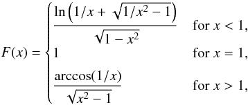 (19)one has
 ![\begin{eqnarray} \Sigma(x) &=& \frac{2\,\Sigma_{\rm s}\,\tau^2}{(\tau^2+1)^2} \Bigg[ \frac{\tau^2+1}{x^2-1}\big(1-F(x)\big)+2\,F(x) \nonumber \\ &&~~ -\frac{\pi}{\sqrt{\tau^2+x^2}}+\frac{\tau^2-1}{\tau\sqrt{\tau^2+x^2}} \log \left(\frac{x}{\sqrt{\tau^2+x^2}+\tau} \right) \Bigg]\cdot \end{eqnarray}](/articles/aa/full_html/2011/07/aa16851-11/aa16851-11-eq61.png) (20)The mean density within a radius x is:
(20)The mean density within a radius x is: ![\begin{eqnarray} &&\bar{\Sigma}(x) = \frac{4\,\Sigma_{\rm s}}{x^2} \frac{\tau^2}{(\tau^2+1)^2} \nonumber\\ &&\times\Bigg\{ \bigg[\tau^2+1+2(x^2-1)\bigg]F(x)+\tau\,\pi +(\tau^2-1)\log\tau \nonumber\\ &&\quad+\sqrt{\tau^2+x^2} \left[ -\pi+\frac{\tau^2-1}{\tau}\log \left(\frac{x}{\sqrt{\tau^2+x^2}+\tau} \right) \right] \Bigg\}\cdot \end{eqnarray}](/articles/aa/full_html/2011/07/aa16851-11/aa16851-11-eq63.png) (21)
(21)
2.3.3. Truncated Non-singular Isothermal profiles
This profile (in the following TNSI) is a truncated and spherical version of the Pseudo-Isothermal Elliptical Mass Distribution (PIEMD) profile by Kassiola & Kovner (1993). Its three dimensional distribution reads: 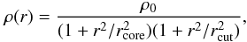 (22)with rcore denoting the profile core radius, and rcut denotes a cutoff radius. The cutoff radius rcut plays a role similar to the truncation radius rtr of the truncated NFW. The surface mass density distribution reads:
 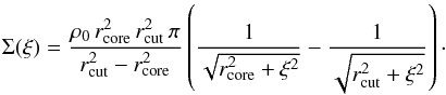 (23)By integrating, one obtains the mean surface mass density
  (24)
(24)
3. Galaxy-galaxy lensing for subhalos
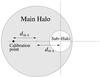 |
Fig. 1 Sketch of a cluster with the main halo and a subhalo with a cluster galaxy at its center. Also shown is the calibration point used to estimate the main halo contribution to the lensing signal around the cluster galaxy and the same distance dM − S from the cluster center. |
Figure 1 shows a schematic view of a galaxy cluster consisting of a cluster main halo and a subhalo. When galaxy-galaxy lensing in its standard form is applied to probe the mass distribution around satellite galaxies (subhalos), the resulting lensing signal has a strong contribution from the cluster main halo.
One can use an analytic model of the main halo to take its contribution into account. However, this relies on strong assumptions about the main halo mass profile. We propose a non-parametric scheme to estimate the main halo contamination and subtract it from the signal. As illustrated in Fig. 2, a calibration point can be used to estimate the contamination from the main halo. The calibration point is located at the same distance dM − S from the main halo center as the subhalo center, but on the opposite side. If the cluster is point-symmetric around its center, we can subtract the signal around the calibration point from the signal around the subhalo, and remove the contamination from the main halo. In the following, we will call this method galaxy-galaxy lensing with calibration (GGLC).
Note, however, that the calibration does not work for very large projected radii ξ. For ξ > 2 × dM − S the method fails since the calibration signal includes the subhalo signal itself. Moreover, as shown in Fig. 2, the signals around the subhalo and the calibration point are very steep for ξ around dM − S. Thus the reconstructed subhalo signal there will be very susceptible to errors introduced by shot noise or the intrinsic ellipticity of the background galaxy. This makes it impossible to reconstruct the subhalo profile for ξ > dM − S in practice.
Since the point-symmetry of any cluster sample is not perfect, our calibration is not only limited from the theoretical point of view. We discuss this in detail in Sect. 5.1.
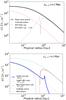 |
Fig. 2 Galaxy-galaxy lensing signals of cluster main halo and subhalo (assuming NFW profiles). The subhalo is at 0.6 Mpc from the cluster center. Top panel: the subhalo around the subhalo center (thin solid red line), the main halo around the main halo center (thick solid black line), and the main halo around the calibration point (dashed/dotted line for positive/negative part). Bottom panel: the subhalo around the subhalo center (thin dotted green line), the subhalo plus main halo around the subhalo center (black dashed line), the subhalo plus main halo around the main halo center (cyan dotted line), the subhalo plus main halo around the calibration point (red solid line), and the reconstructed subhalo (blue thick solid line). |
The excess surface mass density ΔΣsubh(ξ) measured around a sample of lens galaxies can be thought to consist of (at least) two parts. The first contribution is due the (sub)halos of the lenses we are targeting. This part usually dominates the signal close to the lens galaxy. There, ΔΣsubh(ξ) can be interpreted as the excess surface mass density profile of an average lens galaxy halo. The second contribution is due to the (sub)halos of other galaxies, and the clusters’ main halo. This contribution dominates on larger scales. There, ΔΣsubh(ξ) cannot be interpreted directly as the average lens galaxy halo profile.
For a realistic study we need a large sample of clusters, and we do not need each cluster to be perfectly point symmetric. We only need the cluster on average to be sufficiently point-symmetric. In the following the lensing results we present are given by 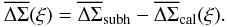 (25)
(25)
4. Simulations
In order to test our proposed galaxy-galaxy lensing method and provide forecasts for the expected signal, we use simulated lensing fields. The fields are obtained by ray-tracing through the Millennium Simulation in combination with mock galaxy catalogs from semi-analytic galaxy formation models.
4.1. The Millennium Simulation
The Millennium Simulation (MS) (Springel et al. 2005) is a large N-body simulation of cosmic structure formation in a flat ΛCDM universe. It uses 21603 dark-matter particles of 8.6 × 10⁸ h-1 M⊙ in a periodic simulation volume of 500 h-1 Mpc side length. The assumed cosmological parameters are: a Hubble constant h = 0.73 (in units of 100 km s-1 Mpc-1), a matter density Ωm = 0.25 and a cosmological constant energy density ΩΛ = 0.75 (in units of the critical density), and a normalization of the matter power spectrum σ8 = 0.9.
An important aspect of the simulation is how structure is defined. All particles which are closer than a certain threshold value are linked. Independent groups of particles are grouped with this Friends of Friends (FOF) algorithm. These FOF groups are considered main halos in the simulation. Substructures within these main halos are identified by the SUBFIND algorithm (Springel et al. 2001): each FOF group is subjected to a gravitational binding analysis, and every group of at least 20 gravitationally bound particles forms a subhalo. The algorithm also estimates a mass MSUBF for each subhalo that equals the total mass of the bound particles4.
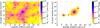 |
Fig. 3 Projected mass maps of a cluster in the MS (left panel) and the synthetic cluster created from it (right panel). |
We define a cluster as a FOF group whose main halo has a mass according to the SUBFIND algorithm larger than 1014M⊙/h. We use this criterion to certify that the selected FOF groups have a large fraction of their mass gravitationally bound and to avoid non-virialized objects.
The MS itself does not take into account baryonic physics. Galaxy formation within the evolving matter distribution of the simulation can however be followed by semi-analytic galaxy formation models (see, e.g., Springel et al. 2001; De Lucia et al. 2004). In this work we use the semi-analytic catalogues by De Lucia & Blaizot (2007) to infer the properties of galaxies in the MS. The model used by them assumes that at the center of every main halo and subhalo there is a galaxy whose evolution is determined by the merging history of the host dark-matter halo and gas-physical processes. These processes are approximated by a set of empirical equations with parameters tuned to make the resulting galaxy population consistent with many observed galaxy properties.
Furthermore, the semi-analytic model allows galaxies whose subhalos has been dissolved during a halo merger event onto a larger halo to survive for some time before merging onto the central galaxy of the main halo. The properties and merging timescales of these orphan galaxies are not known very accurately (from observations or theory), but their contribution to the lensing signal can be significant. In our primary analysis we neglect them. In Sect. 6.2 we discuss how our results are changed if these galaxies are included in the analysis.
4.2. Lensing simulations
The lensing effects caused by the matter structures in the MS are calculated by the multiple-lens-plane ray-tracing algorithm described in Hilbert et al. (2009). The ray-tracing is used to create 128 simulated fields of view of 2 × 2 deg2. Convergence and shear in these fields are stored on regular grids of 40962 pixels in the image plane for multiple source redshifts. In addition, the lensed image properties of all semi-analytic galaxies in each field with stellar masses ≥ 109 h-1 M⊙ are computed. The lens galaxy population for the galaxy-galaxy lensing simulations are selected from these lensed mock galaxy catalogs.
The ray-tracing simulations are also used to compute pixelized maps of the projected surface mass density Σ(β) of thin redshift slices of the simulated lensing light cones. We use these maps first to create simplified mock clusters for performance tests of the calibration method; and second to make a preliminary analysis of our signals.
The source galaxy populations for the galaxy-galaxy lensing simulations are created by randomly drawing image positions within the simulated fields (assuming a uniform spatial distribution in the image plane). The redshifts of the source galaxies are drawn from a distribution (Brainerd et al. 1996)  (26)where α = 2, β = 1.5 and z0 is a function of the median redshift of the survey. We then identify the lens plane that is closest in redshift to each galaxy and interpolate onto it the shear and magnification from the ray-tracing. We add an intrinsic ellipticity to the shear in order to mimic real galaxy images (Eq. (4)). The modulus of the intrinsic ellipticity is drawn from a Gaussian distribution with zero mean and standard deviation σ|ϵi|. In Sect. 5.4.2 we discuss in more detail our simulated lensing catalogues.
4.3. Mock cluster mass maps
To test our calibration scheme, we use a sample of mock clusters. This allows us to know the “true” mass profiles of main halo and subhalos, and thus to quantify how well our method can retrieve these profiles. Since we want to assess the performance of the method in situations as realistic as possible, we use the cluster sample we have from ray-tracing through the Millennium Simulation as a starting point. For each cluster in our cluster sample we create mock clusters at various levels of simplification consisting of an elliptical, or non-elliptical main halo, or no main halo at all.
The main halo of each cluster in the ray-tracing catalog is characterized first by fitting an elliptical truncated NFW profile to the projected mass profile of the cluster5. The resulting mass distribution Σellip(β) is point-symmetric. To create non-symmetric main-halos, the original projected mass Σ(β) of the cluster is first divided by the best-fitting elliptical truncated NFW profile Σellip(β). We then calculate the coefficients ![\begin{equation} \begin{split} a_{\rm n} &= \sum_p \frac{\Sigma(\vbeta_p)}{\Sigma_{\rm ellip}(\vbeta_p)} \cos\left[ n \phi(\vbeta_p) \right],\\ b_{\rm n} &= \sum_p \frac{\Sigma(\vbeta_p)}{\Sigma_{\rm ellip}(\vbeta_p)} \sin\left[ n \phi(\vbeta_p) \right], \end{split} \end{equation}](/articles/aa/full_html/2011/07/aa16851-11/aa16851-11-eq97.png) (27)
(27)
where the index p runs over all pixels in the considered patch. The angle φ(βp) is the polar angle of the pixel from the center of the cluster. The synthetic non-elliptical mass distribution is then ![\begin{eqnarray} \Sigma_{\rm non-el}({\vbeta}_p)&=&\Sigma_{\rm ellip}({\vbeta}_p) \nonumber\\ &&\times {\left( 1+\sum_{n=1}^3\left\{ a_{\rm n}\cos\left[ n \phi(\vbeta_p) \right] +b_{\rm n}\sin\left[ n \phi(\vbeta_p) \right] \right\} \right).} \end{eqnarray}](/articles/aa/full_html/2011/07/aa16851-11/aa16851-11-eq100.png) (28)The mock subhalo profiles are based on the projected mass profiles of subhalos in the MS. We group subhalos in our lensing simulations into bins of subhalo mass MSUBF. Using the proposed calibration method on the projected mass maps, we calculate the bin-averaged excess surface density ΔΣ(ξ) as a function of radius ξ for each bin. We fit NFW profiles to the resulting profiles in the range 0.03 Mpc ≤ ξ ≤ 0.2 Mpc. The relations between the subhalo mass MSUBF and the best-fitting parameters Σs and rs of the NFW profiles are then fit by power laws, yielding
(28)The mock subhalo profiles are based on the projected mass profiles of subhalos in the MS. We group subhalos in our lensing simulations into bins of subhalo mass MSUBF. Using the proposed calibration method on the projected mass maps, we calculate the bin-averaged excess surface density ΔΣ(ξ) as a function of radius ξ for each bin. We fit NFW profiles to the resulting profiles in the range 0.03 Mpc ≤ ξ ≤ 0.2 Mpc. The relations between the subhalo mass MSUBF and the best-fitting parameters Σs and rs of the NFW profiles are then fit by power laws, yielding 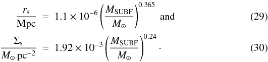
The mass of the NFW profile without truncation diverges if we integrate up to an infinite radius. Therefore, we truncate our halos to make them more realistic. We try different truncation schemes, keeping the former relations for rs and Σs. We experimented with subhalos without truncation, significantly truncated (rtr = 2 rs) and with a truncation above the maximum radius for which we can recover the subhalo lensing signal (rtr = 6.66 rs) in the least massive subhalos.
Each synthetic cluster is constructed by combining the previously described mock main halo and the mock subhalo profiles, whereby the centers of the main halo and the subhalos are used as centers for the mock halos. The mock clusters are then put onto grids having the same resolution as the projected mass maps of the original clusters. Thanks to our procedure, the mock clusters properly take into account
-
the masses and sizes of the main halo and the subhalos;
-
the spatial distribution of the subhalos within the cluster; and
-
the correlation between the main halo shape and the position of the halo center and the subhalos.
An example cluster is shown in Fig. 3.
5. Results
5.1. Performance tests
The method we proposed in Sect. 3 (GGLC) allows theoretically to clean the galaxy-galaxy lensing signal of a subhalo sample from the main halo contamination. Here, we investigate the performance of the method using the synthetic cluster sample. We quantify the range where we can recover the signal below a certain bias and compare it to the reliably range when using the “standard” GGL.
Binning according to MSUBF of all subhalos in clusters for z < 0.9.
We divide the whole mock subhalo sample into several bins according to MSUBF as listed in Table 1. For each bin, we calculate the stacked excess surface mass density profiles ΔΣ(ξ) as a function of projected radius ξ one would obtain if the subhalos were completely isolated. We then compare this “true” profile to the signal measured from our synthetic clusters.
In Fig. 4, we present the difference between GGL and GGLC for one of the truncation schemes. The different truncation schemes offer the same qualitative results. The bias with respect to the true value is reduced in all cases. For the most massive subhalos, comparable in mass to the main halo, the improvement is reduced. On the other hand, for the least massive subhalos the range in radius ξ with a small enough bias doubles. This is a significant improvement for those subhalos which are more subjected to tidal fields and therefore better tracers of the effects that we want to study.
Figure 5 shows the ratio of the measured and true signal for samples of subhalos in the clusters with truncated and non-truncated NFW subhalo profiles and various models for the mass distribution of the cluster main halo. For each mass bin in each panel, we present the results from different situations. We present ΔΣ(ξ) for the following cases: coming only from the subhalos, i.e. the main halo was not added; for an elliptical main halo plus the subhalo population; and from a realistic cluster, using a non-elliptical main halo.
 |
Fig. 4 Ratio of the measured ΔΣ(ξ) to the one we input, using GGLC and standard GGL. The dotted black line, where the ratio is one, is a visual reference. |
 |
Fig. 5 Results from mock clusters. Ratio of the measured ΔΣ(ξ) to the one we input using GGLC, versus the projected physical radius ξ. Top: non-truncated NFWs. Bottom: rtr = 2 rs. We plot only the results for a selection of mass bins, the mass ranges are given. Black dotted-dashed lines: no main halo was added. Red dashed lines: clusters with an elliptical main halo. Blue solid lines: clusters with a non-elliptical main halo. The dotted black line, where the ratio is one, is a visual reference. |
The distribution of the sub-halos is not perfectly point-symmetric with respect the cluster center. When we measure around a particular subhalo, we “see” the surrounding ones and the contribution to our measurement does not average out. This also shows a correlation of the subhalo positions independent of the mass distribution of the main halo.
A completely elliptical halo can always be calibrated properly. The observed difference with respect to the signal with subhalos only, is due to the resolution of our maps (which we also use for the synthetic cluster sample), combined with the sensitivity of the calibration for radii larger than dM−S (Sect. 3). Internal checks were able to verify the source of this discrepancy.
As a compromise between a small bias and a sufficiently large range in ξ, we measure our profiles for those radii where the bias is less than a 10% from the input model. We will only be able to detect a truncation radius if this scale is well inside the range we can measure. The difference between the truncation models does not substantially change the region that we eventually define as suitable to derive the mass profile. Since as we show later on, our simulations do not present a detectable truncation of the mass density profile, we focus in the following on subhalos without truncation.
With GGLC, the measured subhalo profile recovers the true profile within 10% accuracy up to a radius of ~200 kpc for less massive subhalos (with MSUBF ≈ 1011.5 h-1 M⊙ and rs ≈ 0.03 Mpc), and up to ~500 kpc for more massive subhalos (with MSUBF ≈ 1014 h-1 M⊙). We can also see that on scales below 40 kpc, the measured signal is affected by the limited resolution of the synthetic mass maps.
The main halo’s contribution to the bias in ΔΣ(ξ) is more important for subhalos with a small separation from the cluster center dM − S. In fact, including subhalos with a too small dM − S, may decrease the quality of the measured ΔΣ(ξ). Having this in mind, we consider different minimum values for dM − S.
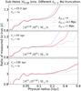 |
Fig. 6 Results from mock clusters, ratio of the measured ΔΣ(ξ) to the one we input, versus the projected physical radius ξ. Only the results for a selection of mass bins, for the case with non-truncated NFWs are presented. The mass ranges are given. Blue dashed lines: whole subhalo sample. Solid red lines: subhalos with dM − S > 0.5 Mpc. Black dashed-dotted lines: subhalos with dM − S > 1 Mpc. The dotted black line, where the ratio is one, is a visual reference. The different selection criteria do not alter significantly the mean rs. |
The results are shown in Fig. 6. Here we present again the ratio of the measured ΔΣ(ξ) to the input value versus physical radius ξ. This time we compare different selections of subhalos. The signal improves if we discard subhalos with dM − S < 0.5Mpc. The most massive subhalos are more likely to be recent mergers and lie far away from the cluster center, so the effect is small in this case (lowest panel).
Increasing the minimal dM − S, depletes the sample and limits our result to subhalos in the outskirts of the cluster. For dM − S < 1Mpc the range where the bias is below 10% increases, but only at the expense of depleting our sample. For the less massive halos, the depletion of the sample worsens the signal. For the most massive subhalos, a larger minimal dM − S improves the results, and seems to be a better choice. Nevertheless, in this work we shall discard subhalos with dM − S < 0.5Mpc, regardless of subhalo type for simplicity. We present the range in ξ defined with our mock clusters for all MSUBF mass bins in Table 2.
5.2. Main halo center detection
Range in radius ξ for which the bias is below 10%, for each subhalo bin according to MSUBF in clusters for z < 0.9.
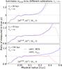 |
Fig. 7 Results from mock clusters, ratio of the measured ΔΣ(ξ) to the one we input, versus the projected physical radius ξ. Only the results for a selection of mass bins, for the case with non-truncated NFWs are presented. The mass ranges are given. Blue solid lines: subhalos with dM − S > 0.5 Mpc, the calibration point was defined using the main halo center. Red dashed lines: subhalos with dM − S > 0.5 Mpc, the calibration point was defined using the average . The dotted black line, where the ratio is one, is a visual reference. The different selection criteria do not alter significantly the mean rs. |
In the Millennium Simulation, we know where the main halo center is, namely in the potential minimum which is always occupied by a BCG. However, in real clusters, the correlation between BCG and the main halo center is supposed to be less tight. The definition of the calibration point is henceforth in principle more difficult.
Our study is targeted at large samples of clusters in optical lensing catalogues. Nonetheless, one could use additional data from other sources like X-rays surveys. Moreover, it should be possible to determine the cluster center accurately from the lensing data itself (Dietrich et al. 2011). Therefore it is not unlikely that a well determined main halo center can be used. For the rest of this work we shall assume the center of the main halo can be well determined. However, for the sake of completeness we want consider the possibility of a BCG displaced from the main halo center and the lack of another more precise way of determining the cluster center.
The expected spatial correlation between the galaxy hosted by the main halo and its center is difficult to determine. In order to quantify the effect of not knowing the main halo center, we compute the calibration, determining the cluster center as a real observer could do. In Fig. 7 we present again, using the synthetic cluster sample, the ratio between the measured signal and the true one, for a selection of sub-halo mass bins.
In blue (solid-line) we plotted the signal previously presented. Then, with a dotted black line, we present the signal where the calibration point is chosen differently. Instead of using the main halo to define the calibration point, we took the average position of all halos in the cluster (main halo and sub-halos), which is also the mean galaxy position. If we assume that the displacements between galaxies and host halos are uncorrelated among themselves, this position can be obtain even if the halos and the hosted galaxies have not a strong correlation. The center of the cluster defined in this way is independent of the possible displacement between the central galaxy and the main halo.
For clusters formed by two large mass overdensities colliding, the separation between the two different centers can be up to ~2 Mpc. The distribution of separations is highly asymmetric, with a mean of 0.215 ± 0.004 and a median of 0.137.
The new way to define the cluster center produce similar results. Note that we only consider galaxies with dM − S > 0.5Mpc, thus we omit the galaxies most sensitive to the change of the cluster center. The range radius that can be used (with an error below 10%) is basicly the same regardless of the chosen center. For the most massive subhalos (lower panel) the new center leads to an over-calibration, which can lead to a misidentification of a truncation radius.
Finally it must be noted that we could select our clusters imposing a maximum distance between the BCG and the average cluster halo position, in order to avoid unrelaxed clusters.
As a conceptually clearer procedure, in the following we use the main halo center (or BCG), to define our calibration.
5.3. Subhalo-galaxy lensing in the Millennium simulation
5.3.1. Subhalo mass profiles for different MSUBF
We now analyze the mass profiles of subhalos in the MS as obtained by applying the GGLC to the projected mass maps from the simulation. The subhalo mass ranges, numbers, and mean masses of the subhalo samples used are listed in Table 3. For the analysis, we only consider subhalos in clusters with redshift z ≤ 0.9 and with dM − S > 0.5Mpc. The resulting average excess surface mass density profiles are shown in Fig. 8.
In order to characterize the subhalo mass profiles we try to find the best fitting model. We consider an NFW profile, a truncated NFW profile and a TNSI profile. For the NFW model, we choose the characteristic surface mass density Σs and the scale radius as free parameters. For the truncated NFW model, we take the truncation radius rtr as additional parameter. For the TNSI model, we fix the core radius rcore = 10-4 Mpc and only fit the cut radius rcut and the central density ρ0. This allows us to analyze the choices made by Limousin et al. (2007) and Natarajan et al. (2007).
We conduct a Bayesian analysis to get the best fitting parameters for each model in each mass bin. We assume a Gaussian likelihood in each case. The corresponding covariance matrices are computed from the data using a bootstrap algorithm. We construct each bootstrap realization by randomly drawing sub-halos with replacements. We do so for each mass bin, producing 10 000 realizations in each case.
Binning of all subhalos in clusters for z < 0.9 according to MSUBF. All subhalos with dM − S > 0.5 Mpc.
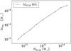 |
Fig. 8 The ΔΣ(ξ) profile measured from the projected mass maps Σ(β), for the different mass bins. Thick lines show the final range used for the analysis. The range in ξ was defined through the test in Sect. 5.1. In dashed black we show the average signal for the host cluster as a visual reference. |
We use the Bayesian evidence to rank the different models. The evidence was computed with a nested sampling algorithm (Skilling 2004). As shown by the results in Table 4, a TNSI is not a suitable model for the subhalos in the MS. Our simulation does not contain baryons, which are expected to change the mass profiles at the innermost regions. Nevertheless, our results raises questions about the choice of the PIEMD model for lensing observations of cluster galaxies. The best model (except for one mass bin, which we consider to be due to statistical fluctuations) is a simple NFW profile. The values for the truncation radii obtained by the fits were in both cases (TNSI and truncated NFW) larger or comparable to the virial radius of the average cluster, and therefore consistent with a lack of a detection.
The errors presented are the standard error from 10 realizations of the measurement except for the leftmost model where we use a raw estimate coming from the algorithm. The analysis in this case did not require a better accuracy. We write in bold the maximum in each case, which belongs to the best model.
From our simulations, it is not possible to detect a truncation radius. A truncation, if present at all, happens at ξ larger than 0.2 Mpc, where our measurements become unreliable due to bias. This is up to four times larger than the truncation radii inferred by Limousin et al. (2007), Natarajan et al. (2007) and Halkola et al. (2007) from lensing data.
Comparison of the logarithm of the evidences for the three models fitted to the ΔΣ signals.
We take the mean of the posterior from the nested sampling algorithm as the best-fitting values for the model parameters, and the posterior standard deviation as parameter errors. The best-fitting values for the concentration c and M200 assuming an NFW profile are presented in Fig. 9. The concentration c slightly decreases with increasing subhalo mass MSUBF. The mass M200 shows a tight and essentially linear relation with the subhalo mass MSUBF. Thus, M200 is a good observable to infer the subhalo mass MSUBF. Note, however, that the mass M200 is always a few times larger than MSUBF. This indicates that the subhalos as defined by SUBFIND do not fully extend to the radius r200.
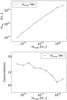 |
Fig. 9 Parameterization of the subhalo profiles using NFW profiles. Bottom panel: concentration concentration as a function of MSUBF. Top panel: M200 as a function of MSUBF. |
The use of M200 as a direct mass estimator on subhalos should be avoided. Otherwise a large fraction of the mass not bound to the subhalo (e.g. nearby subhalos) is attribute to it. We use M200 only as an observable from which we can derive the gravitationally bound mass MSUBF.
In observations, one does not know the radial range at which the GGLC signal can be reliably measured beforehand, since the range depends on the subhalo masses to be inferred from the lensing signal. Here we use the following method to resolve this problem. We infer M200 from the measured GGLC signal in a preliminary radial range, i.e. up to 1 Mpc. Based on the results in Table 5, we use a smaller more adequate range in ξ to measure M200 again and iterate until obtaining consistent results.
5.3.2. Subhalo mass estimation for magnitude-selected subhalo samples
So far, we have only studied mass-selected subhalo samples. We now explore how well one can estimate subhalo masses MSUBF from stacked subhalo samples that are selected according to the magnitudes of the hosted galaxies, which are more amenable to observation.
Binning of all subhalos according to MSUBF in clusters for z < 0.9.
Figure. 10 shows the mass M200 obtained from the GGLC versus the true mean subhalo mass MSUBF for sub-halos binned according to MSUBF, observer-frame absolute r-band magnitude, and observer-frame absolute i-band magnitude. We define 14 bins in luminosity, with a bin width of 0.33 mag, between the values − 19 and − 23.66 for the luminosity or both bands. The relation between the mean inferred mass M200 and mean subhalo mass MSUBF is roughly linear, but noticeably depends on the quantity used for binning. We characterize the relation between M200 and MSUBF by a power law, 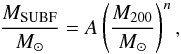 (31)with best-fitting amplitudes A and exponents n listed in Table 6.
The mass-binned and magnitude-binned subhalo samples differ, in particular in the distribution of subhalo masses and mass profiles. As a consequence, even for the same mean subhalo mass MSUBF, the mean profiles may differ substantially. While the averaging to obtain the mean MSUBF and the mean GGLC for each bin is a linear process, the computation of the best fitting parameters and M200 is not. Thus, we may not be able to estimate MSUBF with high precision through M200, but we can derive useful constraints on it.
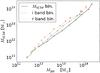 |
Fig. 10 Fitted M200 as a function of average MSUBF for different binnings using the projected mass maps Σ(β). Black solid line: binning according to MSUBF. Dotted red line: binning according to r band absolute observer frame luminosity. Dashed green line: binning according to i band absolute observer frame luminosity. |
5.3.3. Subhalo evolution
In order to observe how subhalos evolve inside the clusters we considered two new parameters, the infall mass Minf and infall time (both computed by Wang et al. 2006). The first is the mass of the main halo that evolved into the current subhalo at the last epoch when it was a central dominant object, i.e. the mass just before it was accreted by a larger structure. The infall time is the moment at which this accretion was detected and allows us to compute the subhalo age, i.e. the time spent inside the cluster at the time of its observation.
We divide our sample into three classes according to Minf, and each of these subhalo classes into three sub-classes according to their age. In order to define the classification, we maximized the signal-to-noise defined as the average ratio (over ξ), between the measured ΔΣ(ξ) and its sample variance (we also avoided too small subhalo samples). The resulting ranges for classes and sub-classes are listed in Table 7. The resulting GGLC signals are shown in Fig. 11.
As shown in Table 7, the mean subhalo masses decrease with increasing subhalo age independent of the considered infall mass range. This is clear evidence for subhalos losing mass inside clusters6. The mass loss is also seen in the subhalo GGLC signals shown in Fig. 11, which also decrease in amplitude at smaller radii with increasing subhalo age. The mean masses M200 inferred from the GGLC signals also reflect the mass loss.
The GGLC profiles also indicate that the mass loss is not due to a simple truncation but rather due to a mass loss at all radii (in the range where the subhalo profiles can be measured reliably), which corroborates the findings of Hayashi et al. (2003). At very large radii, the subhalo profiles tend to increase with increasing subhalo age. This result indicates that the surrounding subhalo’s contribution and main halo asymmetries become more important with increasing subhalo age.
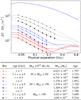 |
Fig. 11 Profiles for different infall mass and time spend inside the cluster: with error bars the regions where the bias is below 10%. The color and the line type are the same for samples selected from the same infall mass range. The symbols are the same for samples defined from the same age bin. In solid blue we plot the average signal for the host cluster as a visual reference. In the table the ranges used for the binning and the average value for each sub-sample. |
Properties of subhalo samples used to study the time evolution of subhalos.
5.4. Forecasts for future surveys
5.4.1. Galaxy observables
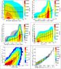 |
Fig. 12 Relations between physical subhalo properties (vertical axis) and observable proxies (horizontal axis). With black frames, we outline those finally used. Contours give the full distribution; we overplot the mean value of each subhalo property and its standard deviation for each bin in the observable (curves with error bars). Top left: age of the subhalo versus the projected radial separation of the subhalo from the main halo center. Top right: age of the subhalo versus redshift-corrected r − i. Middle left: age of the subhalo versus redshift-corrected u − r. See text for a description of the redshift correction. Middle right: age of the subhalo versus our morphology estimator. Bottom left: MSUBF versus absolute r band magnitude. Bottom right: Minf versus stellar mass (using results from Wang et al. 2006). Note that the contour levels differ between the panels. |
Understanding how different observables depend on the underlying subhalo characteristics is essential for obtaining optimal results with our method. We study these relations using the semi-analytic models of galaxy formation in the MS. A discussion of how well the model predicts such relations is beyond the scope of this work. Our aim is to show the feasibility of extracting information with the method we propose. A good review about semi-analytic models is discussed in Baugh (2006) and Benson (2010). Galaxy clustering (Blaizot et al. 2006), galaxy colors and metallicity (Springel et al. 2001) and morphology evolution (De Lucia et al. 2006), just to outline a few examples, have been successfully studied with semi-analytic models.
We only include type-1 galaxies (galaxies with a host subhalo) in our study. We justify our choice in Sect. 6.2.
For our investigation we have studied proxies for the mass as determined by SUBFIND, the infall mass and the age of the subhalos (i.e. the time spent inside the cluster). The results are shown in Fig. 12, where we have marked with a black frame the proxies that show the strongest correlations and are therefore used for our final analysis, for which we only used galaxies hosted by subhalos and imposed an apparent magnitude limit of r < 22.
The age of the subhalos is the most difficult to obtain; none of the observable that we considered displays a strong correlation with this quantity. In top left panel of Fig. 12, we plot the projected radial separation of the subhalo versus its age. Subhalos fall gradually into the main halo through dynamical friction, and so dM − S should be an indicator of the age. However, since the projected separation corresponds to a wide range of three-dimensional separations, we only find a very weak correlation.
In the top right and the middle left panels, we plot the r − i and u − r color indices as a function of subhalo age. The evolution of the stellar population and the depletion of gas to form new stars, make the color of galaxies evolve with time. We account for the redshift evolution of the galaxy colors as follows: we identify for each redshift the red cluster sequence averaged over all clusters, and subtract its mean color from all galaxy colors at the same redshift. By doing this, we can compare galaxies at different redshifts. Both observables are only weakly correlated with the subhalo age. Note that the contour levels are not equally spaced.
The most sensitive proxy for the age of the subhalos is their morphology, which we quantify using the ratio between the luminosities of the bulge and the disk (middle right panel). There are many galaxies which only have a disk component, or only have a bulge (25% of the subhalos in total). In both cases the age of these subhalos cannot be determined. We exclude these galaxies from our analysis, as they should be easy to avoid in real surveys.
The commonly used proxy for mass is luminosity. In the bottom left panel, we plot the r band absolute magnitude as a function of MSUBF. Luminosity in the i bands give qualitatively similar results.
Finally, using results from Wang et al. (2006), we study the stellar mass as a proxy for the infall mass Minf. The result is displayed in the bottom right panel, showing a strong correlation. In the semi-analytic models, galaxies loose their gas rapidly once they become part of a cluster and the star formation effectively stops. Therefore galaxies in clusters maintain on average the stellar mass which they had prior to fall into the cluster, which is then strongly correlated with the halo mass at that time.
5.4.2. Simulated surveys
We now investigate the prospects of measuring the weak lensing signal of subhalos in upcoming surveys. We focus in particular on DES and LSST, but we explore also variations of the main survey characteristics. The area simulated in our ray-tracing is not large enough to represent the total size of the surveys. We are not able, therefore, to reproduce the expected cosmic variance. However, our major concern is the detectability of the signal due to the statistical noise, since we expect that our subhalo samples to be representative. Therefore the influence in the measurements stemming from cosmic variance is assumed to be subdominant.
We create mock galaxy catalogues similar to those expected from these surveys. As described in Sect. 4.2, the redshift distribution of our sources follows that of Brainerd et al. 1996. The modulus of the intrinsic ellipticity is drawn from a Gaussian distribution with zero mean and standard deviation σ|ϵi|. This intrinsic ellipticity is the dominant source of noise in our measurement, resulting in an error in the measurement ∝  , where n is the total number of foreground-background galaxy pairs used to measure the final ΔΣ(ξ). For a single galaxy, we assume σ|ϵi| = 0.3. However, the survey areas of DES and LSST are considerably larger than the area covered by the ray-tracing. In order to simulate these surveys with their larger number of background galaxies, we therefore use a effective intrinsic ellipticity variance, which is reduced by the ratio of the survey area to the area of the simulations
 .
.
For the lens sample, we impose a maximum redshift of z = 0.9. Subhalos at higher redshift are difficult to probe with lensing since there are fewer background sources available. Henceforth, their inclusion offers no improvement in the detectability of the signal. For the LSST-like survey, we only considered lens galaxies with r < 26 in apparent magnitude, for the other three surveys is r < 22. We divide these samples further into 14 bins in absolute r-band magnitude ranging from r = −23.66 to r = −19 with a bin width of 0.33 mag.
The details of these surveys are summarized in Table 8. The LSST and the DES surveys are expected to be around 10% larger in size than the ones that we effectively consider here. In this way, we account for the reduction of the usable area due to masking. Furthermore, with the ficticious DES-WIDE survey we analyze the impact of having a survey like DES but with the solid angle of LSST, and with the INT survey the effect of having deeper observations on the same area as DES.
Parameters for the different surveys considered in our detectability study.
For simplicity, in the following the errors plotted are the combined standard errors obtained from ΣSubh and Σcal. We assessed that the correlation between ΣSubh and Σcal is subdominant. However, for the parameter fitting we use the full covariance matrix computed with bootstrapping in each case.
5.4.3. Signal-to-noise ratio
For each survey and luminosity bin, we compute a mean signal-to-noise ratio (SNR) by averaging over eight logarithmic bins in projected radius ξ in the range from 0.043 to 0.12 Mpc: ![\begin{equation} SNR= \left\langle \frac{\epsilon_{\rm t}(\xi)}{\sigma\left[\epsilon_{\rm t}(\xi)\right]} \right\rangle_{\xi}\cdot \end{equation}](/articles/aa/full_html/2011/07/aa16851-11/aa16851-11-eq256.png) (32)We use for σ[ϵt(ξ)] the combined standard error of the mean ΣSubh and Σcal. These SNR values neither take into account correlated noise nor express how well a particular feature can be detected. Nonetheless, they are compact estimators and offer a rule of thumb for the expected signal quality.
(32)We use for σ[ϵt(ξ)] the combined standard error of the mean ΣSubh and Σcal. These SNR values neither take into account correlated noise nor express how well a particular feature can be detected. Nonetheless, they are compact estimators and offer a rule of thumb for the expected signal quality.
In Fig. 13, we present the resulting SNR values for the four surveys considered. Luminous galaxies usually have a larger halo with a stronger signal, whereas faint galaxies are more numerous, corresponding to a smaller statistical error. The SNR depends on these two competing effects, resulting in a maximum of the SNR signal-to-noise ratios are around − 21.5 mag.
The least luminous bins are below the two-sigma level in all surveys except for LSST; in these cases, the signal-to-noise ratio can be improved by using broader bins.
Finally, in the left panel of Fig. 14, we present the predicted galaxy-galaxy lensing signals for a LSST-like survey, and in the right panel for a DES-like survey. The signal-to-noise is lower in a DES-like survey, requiring the use of fewer luminosity bins (from r = −24.25 to r = 19 with a width of 0.75 mag) than for LSST. This figure presents a global characterization of the expected signals, taking into account an adequate treatment of the galaxy samples. We can see the quality of the signals and how detailed our models can be.
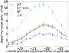 |
Fig. 13 Our compact SNR estimator, for the different luminosity bins for each mock survey considered. For each luminosity bin we plot the mean magnitude. The errors plotted are standard errors obtained from the sample. |
5.4.4. Mass-luminosity relation
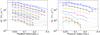 |
Fig. 14 Measured ΔΣ(ξ) profiles of galaxies binned by r-band absolute magnitude. Left panel: LSST-like survey, with r < 26 in apparent magnitude. Right panel: DES-like survey, with r < 22 in apparent magnitude. Error bars show the data used for the analysis later on, the range was derive from our results in Table 5. The solid blue line without error bars is the measurement for the host cluster shown as a visual reference. |
We now address the question how well a mass-luminosity relation for subhalos can be estimated from DES and LSST. The measurement of such a relation can help to distinguish between models of sub-structure formation. As we probe larger scales than stellar dynamics, and we consider large samples of galaxies compared to strong lensing analyses, our method is largely complementary to other methods. In Fig. 14 we present the results for DES and LSST. Note that we only plot error bars for the range where we consider our measure has a bias below 10%.
In order to obtain the subhalo mass MSUBF, one needs to derive M200 from the measured ΔΣ profiles. The subhalo mass can then be computed from a scaling relation between MSUBF and M200, which is shown in the top panel of Fig. 15. The final mass-luminosity relations, for both a LSST and a DES-like survey, are shown in Fig. 16. Using DES or LSST, one can constrain the mass-luminosity relation over two decades in mass. The systematic differences between the relation for the two surveys can be explained by the different lens samples used. The brightest bins are populated with the same objects for both surveys and therefore the scaling relations are similar. At the fainter end, the different magnitude cuts in combination with the broader luminosity bins in the DES change the mass-luminosity relation (Fig. 15, bottom panel).
Nonetheless, the relation between M200 and the mass is the same (within the errors) in both cases. The smaller number density of faint galaxies in DES compared to the LSST survey reduces in this case the range over which we can measure the mass-luminosity relation. Note that the faintest luminosity bin for the DES-like survey may not be usable as the measurement error becomes too large.
5.4.5. Evolution of subhalo profiles
In Sect. 5.3.3, we showed how the subhalo mass profiles change with time and found that it is not possible to detect a truncation in the original sense, and that the mass density decreased at all scales consistent with a heating process. We now study whether this behavior can be detected with DES or LSST using observable quantities only.
In Fig. 17, the predicted galaxy-galaxy lensing signals for both LSST (left panel) and DES (right panel) are shown with different symbols for the different stellar mass bins. Additionally, we have divided each of the stellar mass bins into two subsets according to morphology. The details of the binning in morphology and stellar mass are given in tables inside the figure.
The dashed red lines belong to galaxies with a relatively large bulge, which should belong to old subhalos. With blue dotted lines we plotted the signals from galaxies with a large disk, which should belong to younger subhalos. The number of stellar mass bins we can analyze is limited, since we need to split them further into early-type and late-type galaxies. The stellar mass ranges were obtained by experimentation; in the case of the DES-like survey we focused on a particular range where the effect was strongest. Note that we only plot error bars for the range where our measurement has a bias below 10%.
The sub-division according to morphology does not always produce the desired results. One can see from the last two rows in the top table, that for the most massive satellite galaxies, the infall mass (eighth column) of the two morphology bins are very different. Older subhalos have a significantly larger mean infall mass, which indicates that they evolved in a different manner. This difference masks any possible detection of mass loss due to tidal stripping by the cluster.
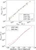 |
Fig. 15 Top: relation between the fitted parameter M200 and MSUBF. Bottom: the mass-luminosity relation obtained from the catalogues. We plot in solid black the results for a DES-like survey, and in dashed red for a LSST-like survey. |
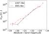 |
Fig. 16 Bottom: the relation between the fitted parameter M200 and the luminosity in absolute observer frame r band magnitude. We plot in solid black the results for a DES-like survey, and in dashed red for a LSST-like survey. |
With the exception of this particular bin, however, Fig. 17 shows that the profile amplitude of bulge-dominated galaxies is smaller than the one of disk-dominated objects, in accordance with our predictions from Sect. 5.3.3. This can be detected with high significance in the LSST; for the DES-like survey the detection is hampered by the low signal-to-noise ratio.
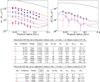 |
Fig. 17 Morphology-stellar mass classification for a LSST-like survey (left panel) and for a DES-like survey (right panel). The black solid line is the measurement for the host cluster shown for visual reference. We only plot symbols and error bars for the range where we consider that the bias is below 10%. The subhalos are at dM − S > 0.5 Mpc. Blue dotted lines correspond to galaxies with a relatively small bulge: Disk → 0 < LBulge/LTotal ≤ 0.6. Red dashed lines correspond to galaxies with a large bulge which spent more time inside a cluster: Bulge → 0.6 < LBulge/LTotal < 0.98. The different symbols distinguish different stellar mass bins (in units of 1010 M⊙). For the left panel the ranges are: 1 → [0.14:1.4 ] , II → [1.4:4.11 ] , III → [4.11:10.96 ] , 4 → [10.96:∞ ] . For the right panel the ranges are I → [1.1:4.1 ] , II → [4.1:13.7 ] . |
6. Systematic effects
6.1. Validity of the weak lensing approximation
So far, we have assumed that the weak lensing approximation is valid in our measurements, i.e. that κ ≪ 1 and thus that the reduced shear effectively equals the shear. To check the validity of this approximation, we compare the galaxy-galaxy lensing signal of subhalos measured using shear with the signal obtained using reduced shear.
In Fig. 15 we have estimated M200 by fitting NFW profiles to the ΔΣ profiles measured from galaxy catalogues obtained from the full ray-tracing using the shear γ(θ) and from similar catalogues using the reduced shear g(θ). No significant difference between the two methods is found. For the average subhalo, the impact of the environment is not important. Within internal checks, we have observed a significant discrepancy only for the most massive subhalos for the innermost radii. This is produced by the large convergence of the subhalo itself and not related to the host main halo.
6.2. Type-2 galaxies
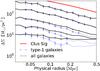 |
Fig. 18 Excess surface mass density ΔΣ(ξ) for a few luminosity bins for an LSST-like survey. The blue dashed lines correspond to the measurements only for type-1 galaxies. The solid black lines correspond to the combination of both type-1 and type-2 galaxies. The range where we assume the measurement has a bias below 10% is highlighted (derived using our results for type-1 only profiles). The solid thick red line is the signal for the average cluster, shown for visual reference. |
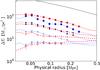 |
Fig. 19 Morphology-stellar mass classification for a LSST-like survey including both type-1 and type-2 galaxies. Blue dotted lines correspond to galaxies with a relatively small bulge, red dashed to those with a large bulge. The different symbols distinguish different stellar mass bins. The range where we assume the measurement has a bias below 10% is highlighted (derived using our results from the type-1 only profiles). The classification ranges are described in the top table in Fig. 17. The black solid line is the measurement for the host cluster shown for visual reference. |
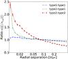 |
Fig. 20 Ratio between the galaxy number density around a galaxy and around its corresponding calibration point, as a function of distance. We also plot as visual reference the line where the ratio is 1. Dotted-dashed red: excess type-2 number density around type-2. Solid blue: type-1 number density around type-1. Green dashed: excess type-1 number density around type-2. dM − S > 0.5 Mpc. |
The semi-analytic model of galaxy formation by De Lucia & Blaizot (2007) contains galaxies that have “lost” their subhalos. Whenever a subhalo is no longer detected (e.g. because it has lost most of its mass due to tidal stripping), the hosted galaxy is still maintained and placed at the position of the most bound particle of the former subhalo. After the dynamical friction timescale, these galaxies eventually disappear as they merge into the main halo galaxy.
The results presented so far were computed excluding type-2 galaxies for the following reasons:
-
they are hosted by subhalos below or around the mass resolutionlimit;
-
they exist under the assumption that the stripping of a large part of the subhalo does not destroy the hosted galaxy;
-
the survival time is heavily influenced by the model.
Nevertheless, to understand the impact of such galaxies on our measurements, we analyze how our results are altered when including them. We present how our measurements would be affected assuming that type-2 are real and that we cannot distinguish between them and type-1 galaxies.
In Fig. 18, we present ΔΣ(ξ) for a selection of luminosity bins for type-1 galaxies (with dashed blue lines) and the same luminosity bins but for the combination of type-2 and type-1 galaxies (with solid black lines). The inclusion of type-2 galaxies change the average profile, especially at large radii. The change is larger for fainter galaxies. The new profiles are flatter, and there is a systematic error in the determination of the mass profile. This effect can also interfere with our ability to assign any kind of mass estimate.
In Fig. 19, we present the same analysis as in the top panel in Fig. 17, but with both type-2 and type-1 galaxies. Recall that the line and color type encodes the morphology (as a proxy for the subhalos’ age), and the symbol encodes the stellar mass (as a proxy for the subhalo infall mass). The inclusion of type-2 galaxies is more important if we aim to estimate the mass loss on subhalos induced by tidal stripping. Our former ability to measure this effect was small, and the change in the profiles that type-2 galaxies produce makes it impossible.
We are able to trace the mass responsible for the lensing signal in type-2 galaxies. In Fig. 20, we quantify how likely is to find a companion near a type-2 galaxy. We compare the number density as function of radius, around a galaxy and its calibration point. Type-2 galaxies are on average close to a subhalo which accounts for the lensing signal measured. We were able as well to detect type-2 galaxies associated with projected overdensities which were not detected as subhalos by SUBFIND.
The presence of galaxies with no halos makes our measurements less precise. However, if such galaxies exists, we could use our analysis to determine the fraction of galaxies of such type, and to distinguish them from galaxies with a host halo.
7. Summary and conclusions
In order to understand the evolution of galaxy clusters, it is essential to study the matter profiles of satellite galaxies. Analyzing how these profiles evolve with time can improve our knowledge on galaxy evolution and on structure formation.
In this work we analyzed the use of weak gravitational lensing on satellite galaxies inside clusters, in particular the use of galaxy-galaxy lensing. With this probe, we can measure in a non-parametric way the average projected mass profiles of the host matter halos of galaxies. This cosmological probe correlates the image distortion (shear) of a background galaxy with the mass of a foreground galaxy.
Galaxy-galaxy lensing needs large galaxy samples. For this reason it has not yet been fully exploited on cluster satellite galaxies. In our work, we forecast results for future surveys using the Millennium Simulation (Springel et al. 2005), ray-tracing simulations (Hilbert et al. 2009) and the galaxy semi-analytic catalogues by De Lucia & Blaizot (2007).
We presented the details of galaxy-galaxy lensing measurements on satellite galaxies and its contamination from the host cluster. In order to overcome the contamination from the host cluster we proposed a calibration method, which can solve the problem up to a certain range in radius. For each subhalo, we define a point at the same distance from the main halo as the subhalo, but in the opposite direction as seen from the cluster center. We can estimate the contribution of the main halo by measuring the tangential shear around this new point, under the assumption that the cluster is point-symmetric.
We created mass maps of our clusters using theoretical profiles with known parameters. With this mock cluster sample we were able to test our calibration method taking into account realistic characteristics for our cluster samples such as halo spatial distribution or mass function. We estimated the performance of our measurements at different radii and we defined a minimal separation between the subhalo and the main halo center to optimize the signals.
With the previous tests, we could characterize the subhalos in the Millennium Simulation using projected mass maps. The weak lensing signal of subhalos is well described by a simple NFW profile, and it was not possible to detect a truncation radius. Our results are consistent with an abrupt truncation of the mass profile at radii larger than 0.2 Mpc. There are certain discrepancies between our work and the previously published works from Limousin et al. (2007), Natarajan et al. (2007), Halkola et al. (2007) and Suyu & Halkola (2010). These authors measured a much smaller extent of the subhalos using gravitational lensing on a few observed clusters. The results were derived using parametric models for the mass profiles of the subhalos and the main halo. The models used by these authors do not fit subhalos in the Millennium Simulation. Since the Millennium Simulation only contains dark matter, there is not absolute certainty that NFW profiles should be the best description for halos of real galaxies. On the other hand our method did not include strong lensing constraints in comparison to the previous works. Nevertheless, our results challenge the choices made in the afore-mentioned works. The truncation radii that they measured can be also interpreted as a consequence of the parametric method used. Therefore, further analysis and better data are needed in order to solve the problem.
We also were able to characterize the evolution of the mass profiles. We showed that the lensing profiles decrease in amplitude with time. This is consistent with a mass loss at all scales. Due to the tidal forces exerted by the host halo, subhalos are stripped of the mass at the outermost radii, and at the same time the mass at the inner regions is redistributed. This is consistent with the work by Hayashi et al. (2003) and also supports the idea of large truncation radii.
After describing the subhalo profiles we used simulated galaxy catalogues to forecast signals for future surveys, focusing on DES (The Dark Energy Survey Collaboration 2005) and LSST (Ivezic et al. 2009). We analyzed the semi-analytic catalogues in order to classify the galaxy samples to optimize the measurements. With the result from this analysis we derived the following results.
We predict the detectability of the signals using a compact estimator of the signal-to-noise ratio. The cluster sample required is very large, but we can already expect signals from a DES-like survey roughly above the three sigma level. The data from a LSST-like survey is well-suited for the studies that we proposed.
There is not a unique way of separating between subhalo and host halo mass. In this work, we considered that the mass of the subhalo is well estimated in our simulations by the SUBFIND algorithm (Springel et al. 2001) (MSUBF). We modeled the relation between the measured NFW profiles and the gravitationally bound mass of the subhalo mass MSUBF. We also checked that the weak lensing approximation is valid.
According to the semi-analytic catalogues, luminosity in the SDSS r band is a good proxy for mass. We predict that it is possible even for a DES-like survey to constrain the mass-luminosity relations of subhalos over two decades in mass, from around 5 × 10¹¹ to 1014M⊙.
In order to study the time evolution of the profiles using realistic data, we binned the galaxies according the mass of the subhalo prior to falling into the cluster and the time spent inside the cluster (subhalo age). Within the semi-analytic catalogues, it is possible to infer their initial mass from their observed stellar mass. On the other hand we could not find any galaxy observable that is strongly correlated with the subhalo age. With these observables, we could only put weak constraints to the evolution of subhalo matter profiles.
In our analyses we neglected galaxies without a host subhalo which one finds in the semi-analytic catalogues of De Lucia & Blaizot (2007). A priori, these galaxies are not fully reliable as they populate mass overdensities below the resolution limit of the Millennium Simulation. Nevertheless, for completeness we considered their influence. These galaxies show a lensing signal with a high amplitude, which can be explained as being produced by correlated halos. We also were able to quantify the correlation between the position of type-2 galaxies and other subhalos. Finally, we presented how our previous analysis is affected by assuming that these galaxies are realistic and that we are not able to distinguish them from galaxies with a host subhalo. However, further simulations are needed in order to investigate galaxies of such characteristics.
Note, that there is no unique way of estimating the mass of a subhalo, and that even the same algorithm gives different values depending on the subhalo position inside the main halo (Muldrew et al. 2011).
Projected NFW profiles have been shown to be a good fit for projected cluster halo profiles of the Millennium Simulation (Hilbert & White 2010).
Acknowledgments
We thank Lan Wang for providing the infall mass and infall snapshot catalogues for this project. We thank Tim Eifler for moral support and comments, and Simon White for his comments. E.P.M. acknowledges support by the Argelander-Institut für Astronomie and by the EU Project DUEL, Projektnr. 36133. J.H. and S.H. acknowledge support by the Deutsche
Forschungsgemeinschaft within the Priority Programme 1177 under the project SCHN 342/6 and the Transregional Collaborative Research Centre TRR 33 “The Dark Universe”. The Millennium Simulation databases used in this paper and the web application providing online access to them were constructed as part of the German Astrophysical Virtual Observatory.
References
- Baltz, E. A., Marshall, P., & Oguri, M. 2009, J. Cosm. Astro-Particle Phys., 1, 15 [Google Scholar]
- Bartelmann, M. 1996, A&A, 313, 697 [NASA ADS] [Google Scholar]
- Bartelmann, M., & Schneider, P. 2001, Phys. Rep., 340, 291 [NASA ADS] [CrossRef] [Google Scholar]
- Baugh, C. M. 2006, Rep. Prog. Phys., 69, 3101 [NASA ADS] [CrossRef] [Google Scholar]
- Benjamin, J., Heymans, C., Semboloni, E., et al. 2007, MNRAS, 381, 702 [NASA ADS] [CrossRef] [Google Scholar]
- Benson, A. J. 2010, Phys. Rep., 495, 33 [NASA ADS] [CrossRef] [Google Scholar]
- Blaizot, J., Szapudi, I., Colombi, S., et al. 2006, MNRAS, 369, 1009 [NASA ADS] [CrossRef] [Google Scholar]
- Bradač, M., Clowe, D., Gonzalez, A. H., et al. 2006, ApJ, 652, 937 [NASA ADS] [CrossRef] [Google Scholar]
- Brainerd, T. G., Blandford, R. D., & Smail, I. 1996, ApJ, 466, 623 [NASA ADS] [CrossRef] [Google Scholar]
- Clowe, D., Bradač, M., Gonzalez, A. H., et al. 2006, ApJ, 648, L109 [NASA ADS] [CrossRef] [Google Scholar]
- De Lucia, G., & Blaizot, J. 2007, MNRAS, 375, 2 [NASA ADS] [CrossRef] [Google Scholar]
- De Lucia, G., Kauffmann, G., & White, S. D. M. 2004, MNRAS, 349, 1101 [NASA ADS] [CrossRef] [Google Scholar]
- De Lucia, G., Springel, V., White, S. D. M., Croton, D., & Kauffmann, G. 2006, MNRAS, 366, 499 [NASA ADS] [CrossRef] [Google Scholar]
- Dietrich, J. P., Böhnert, A., Lombardi, M., Hilbert, S., & Hartlap, J. 2011, MNRAS, submitted [arXiv:1103.4607] [Google Scholar]
- Fu, L., Semboloni, E., Hoekstra, H., et al. 2008, A&A, 479, 9 [Google Scholar]
- Ghigna, S., Moore, B., Governato, F., et al. 1998, MNRAS, 300, 146 [NASA ADS] [CrossRef] [Google Scholar]
- Ghigna, S., Moore, B., Governato, F., et al. 2000, ApJ, 544, 616 [NASA ADS] [CrossRef] [Google Scholar]
- Halkola, A., Seitz, S., & Pannella, M. 2006, MNRAS, 372, 1425 [NASA ADS] [CrossRef] [Google Scholar]
- Halkola, A., Seitz, S., & Pannella, M. 2007, ApJ, 656, 739 [NASA ADS] [CrossRef] [Google Scholar]
- Halkola, A., Hildebrandt, H., Schrabback, T., et al. 2008, A&A, 481, 65 [NASA ADS] [CrossRef] [EDP Sciences] [Google Scholar]
- Hayashi, E., Navarro, J. F., Taylor, J. E., Stadel, J., & Quinn, T. 2003, ApJ, 584, 541 [NASA ADS] [CrossRef] [Google Scholar]
- Hilbert, S., & White, S. D. M. 2010, MNRAS, 404, 486 [NASA ADS] [Google Scholar]
- Hilbert, S., Hartlap, J., White, S. D. M., & Schneider, P. 2009, A&A, 499, 31 [NASA ADS] [CrossRef] [EDP Sciences] [Google Scholar]
- Hoekstra, H., Yee, H. K. C., & Gladders, M. D. 2004, ApJ, 606, 67 [NASA ADS] [CrossRef] [Google Scholar]
- Israel, H., Erben, T., Reiprich, T. H., et al. 2010, A&A, 520, A58 [NASA ADS] [CrossRef] [EDP Sciences] [Google Scholar]
- Ivezic, Z., Tyson, J. A., Allsman, R., et al. 2009, Bull. Am. Astron. Soc., 41, 366 [Google Scholar]
- Jee, M. J., Rosati, P., Ford, H. C., et al. 2009, ApJ, 704, 672 [NASA ADS] [CrossRef] [Google Scholar]
- Kassiola, A., & Kovner, I. 1993, ApJ, 417, 450 [NASA ADS] [CrossRef] [Google Scholar]
- Komatsu, E., Smith, K. M., Dunkley, J., et al. 2011, ApJS, 192, 18 [NASA ADS] [CrossRef] [Google Scholar]
- Limousin, M., Kneib, J. P., Bardeau, S., et al. 2007, A&A, 461, 881 [NASA ADS] [CrossRef] [EDP Sciences] [Google Scholar]
- Mandelbaum, R., Seljak, U., Kauffmann, G., Hirata, C. M., & Brinkmann, J. 2006, MNRAS, 368, 715 [Google Scholar]
- Mandelbaum, R., Seljak, U., & Hirata, C. M. 2008, J. Cosmology Astropart. Phys., 8, 6 [Google Scholar]
- Muldrew, S. I., Pearce, F. R., & Power, C. 2011, MNRAS, 410, 2617 [NASA ADS] [CrossRef] [Google Scholar]
- Natarajan, P., De Lucia, G., & Springel, V. 2007, MNRAS, 376, 180 [NASA ADS] [CrossRef] [Google Scholar]
- Navarro, J. F., Frenk, C. S., & White, S. D. M. 1997, ApJ, 490, 493 [NASA ADS] [CrossRef] [Google Scholar]
- Okabe, N., Takada, M., Umetsu, K., Futamase, T., & Smith, G. P. 2010, PASJ, 62, 811 [NASA ADS] [Google Scholar]
- Parker, L. C., Hoekstra, H., Hudson, M. J., van Waerbeke, L., & Mellier, Y. 2007, ApJ, 669, 21 [Google Scholar]
- Percival, W. J., Reid, B. A., Eisenstein, D. J., et al. 2010, MNRAS, 401, 2148 [NASA ADS] [CrossRef] [Google Scholar]
- Riess, A. G., Macri, L., Casertano, S., et al. 2009, ApJ, 699, 539 [NASA ADS] [CrossRef] [Google Scholar]
- Schirmer, M., Suyu, S., Schrabback, T., et al. 2010, A&A, 514, A60 [NASA ADS] [CrossRef] [EDP Sciences] [Google Scholar]
- Schneider, P. 2006, in Saas-Fee Advanced Course 33: Gravitational Lensing: Strong, Weak and Micro, ed. G. Meylan, P. Jetzer, P. North, P. Schneider, C. S. Kochanek, & J. Wambsganss, 269 [Google Scholar]
- Schneider, P., Kochanek, C., & Wambsganss, J. 2006, Gravitational Lensing: Strong, Weak and Micro, Saas-Fee Advanced Course 33 (Berlin: Springer) [Google Scholar]
- Schrabback, T., Hartlap, J., Joachimi, B., et al. 2010, A&A, 516, A63 [NASA ADS] [CrossRef] [EDP Sciences] [Google Scholar]
- Sheldon, E. S., Johnston, D. E., Masjedi, M., et al. 2009, ApJ, 703, 2232 [NASA ADS] [CrossRef] [Google Scholar]
- Simon, P., Watts, P., Schneider, P., et al. 2008, A&A, 479, 655 [NASA ADS] [CrossRef] [EDP Sciences] [Google Scholar]
- Skilling, J. 2004, in Am. Inst. Phys. Conf. Ser., 735, ed. R. Fischer, R. Preuss, & U. V. Toussaint, 395 [Google Scholar]
- Springel, V., White, S. D. M., Tormen, G., & Kauffmann, G. 2001, MNRAS, 328, 726 [Google Scholar]
- Springel, V., White, S. D. M., Jenkins, A., et al. 2005, Nature, 435, 629 [NASA ADS] [CrossRef] [PubMed] [Google Scholar]
- Suyu, S. H., & Halkola, A. 2010, A&A, 524, A94 [NASA ADS] [CrossRef] [EDP Sciences] [Google Scholar]
- The Dark Energy Survey Collaboration. 2005 [arXiv:astro-ph/0510346] [Google Scholar]
- Tian, L., Hoekstra, H., & Zhao, H. 2009, MNRAS, 393, 885 [NASA ADS] [CrossRef] [Google Scholar]
- Wang, L., Li, C., Kauffmann, G., & De Lucia, G. 2006, MNRAS, 371, 537 [NASA ADS] [CrossRef] [Google Scholar]
- Wright, C. O., & Brainerd, T. G. 2000, ApJ, 534, 34 [NASA ADS] [CrossRef] [Google Scholar]
- Yang, X., Mo, H. J., van den Bosch, F. C., et al. 2006, MNRAS, 373, 1159 [NASA ADS] [CrossRef] [Google Scholar]
All Tables
Range in radius ξ for which the bias is below 10%, for each subhalo bin according to MSUBF in clusters for z < 0.9.
Binning of all subhalos in clusters for z < 0.9 according to MSUBF. All subhalos with dM − S > 0.5 Mpc.
Comparison of the logarithm of the evidences for the three models fitted to the ΔΣ signals.
All Figures
|
Fig. 1 Sketch of a cluster with the main halo and a subhalo with a cluster galaxy at its center. Also shown is the calibration point used to estimate the main halo contribution to the lensing signal around the cluster galaxy and the same distance dM − S from the cluster center. |
| In the text | |
|
Fig. 2 Galaxy-galaxy lensing signals of cluster main halo and subhalo (assuming NFW profiles). The subhalo is at 0.6 Mpc from the cluster center. Top panel: the subhalo around the subhalo center (thin solid red line), the main halo around the main halo center (thick solid black line), and the main halo around the calibration point (dashed/dotted line for positive/negative part). Bottom panel: the subhalo around the subhalo center (thin dotted green line), the subhalo plus main halo around the subhalo center (black dashed line), the subhalo plus main halo around the main halo center (cyan dotted line), the subhalo plus main halo around the calibration point (red solid line), and the reconstructed subhalo (blue thick solid line). |
| In the text | |
|
Fig. 3 Projected mass maps of a cluster in the MS (left panel) and the synthetic cluster created from it (right panel). |
| In the text | |
|
Fig. 4 Ratio of the measured ΔΣ(ξ) to the one we input, using GGLC and standard GGL. The dotted black line, where the ratio is one, is a visual reference. |
| In the text | |
|
Fig. 5 Results from mock clusters. Ratio of the measured ΔΣ(ξ) to the one we input using GGLC, versus the projected physical radius ξ. Top: non-truncated NFWs. Bottom: rtr = 2 rs. We plot only the results for a selection of mass bins, the mass ranges are given. Black dotted-dashed lines: no main halo was added. Red dashed lines: clusters with an elliptical main halo. Blue solid lines: clusters with a non-elliptical main halo. The dotted black line, where the ratio is one, is a visual reference. |
| In the text | |
|
Fig. 6 Results from mock clusters, ratio of the measured ΔΣ(ξ) to the one we input, versus the projected physical radius ξ. Only the results for a selection of mass bins, for the case with non-truncated NFWs are presented. The mass ranges are given. Blue dashed lines: whole subhalo sample. Solid red lines: subhalos with dM − S > 0.5 Mpc. Black dashed-dotted lines: subhalos with dM − S > 1 Mpc. The dotted black line, where the ratio is one, is a visual reference. The different selection criteria do not alter significantly the mean rs. |
| In the text | |
|
Fig. 7 Results from mock clusters, ratio of the measured ΔΣ(ξ) to the one we input, versus the projected physical radius ξ. Only the results for a selection of mass bins, for the case with non-truncated NFWs are presented. The mass ranges are given. Blue solid lines: subhalos with dM − S > 0.5 Mpc, the calibration point was defined using the main halo center. Red dashed lines: subhalos with dM − S > 0.5 Mpc, the calibration point was defined using the average . The dotted black line, where the ratio is one, is a visual reference. The different selection criteria do not alter significantly the mean rs. |
| In the text | |
|
Fig. 8 The ΔΣ(ξ) profile measured from the projected mass maps Σ(β), for the different mass bins. Thick lines show the final range used for the analysis. The range in ξ was defined through the test in Sect. 5.1. In dashed black we show the average signal for the host cluster as a visual reference. |
| In the text | |
|
Fig. 9 Parameterization of the subhalo profiles using NFW profiles. Bottom panel: concentration concentration as a function of MSUBF. Top panel: M200 as a function of MSUBF. |
| In the text | |
|
Fig. 10 Fitted M200 as a function of average MSUBF for different binnings using the projected mass maps Σ(β). Black solid line: binning according to MSUBF. Dotted red line: binning according to r band absolute observer frame luminosity. Dashed green line: binning according to i band absolute observer frame luminosity. |
| In the text | |
|
Fig. 11 Profiles for different infall mass and time spend inside the cluster: with error bars the regions where the bias is below 10%. The color and the line type are the same for samples selected from the same infall mass range. The symbols are the same for samples defined from the same age bin. In solid blue we plot the average signal for the host cluster as a visual reference. In the table the ranges used for the binning and the average value for each sub-sample. |
| In the text | |
|
Fig. 12 Relations between physical subhalo properties (vertical axis) and observable proxies (horizontal axis). With black frames, we outline those finally used. Contours give the full distribution; we overplot the mean value of each subhalo property and its standard deviation for each bin in the observable (curves with error bars). Top left: age of the subhalo versus the projected radial separation of the subhalo from the main halo center. Top right: age of the subhalo versus redshift-corrected r − i. Middle left: age of the subhalo versus redshift-corrected u − r. See text for a description of the redshift correction. Middle right: age of the subhalo versus our morphology estimator. Bottom left: MSUBF versus absolute r band magnitude. Bottom right: Minf versus stellar mass (using results from Wang et al. 2006). Note that the contour levels differ between the panels. |
| In the text | |
|
Fig. 13 Our compact SNR estimator, for the different luminosity bins for each mock survey considered. For each luminosity bin we plot the mean magnitude. The errors plotted are standard errors obtained from the sample. |
| In the text | |
|
Fig. 14 Measured ΔΣ(ξ) profiles of galaxies binned by r-band absolute magnitude. Left panel: LSST-like survey, with r < 26 in apparent magnitude. Right panel: DES-like survey, with r < 22 in apparent magnitude. Error bars show the data used for the analysis later on, the range was derive from our results in Table 5. The solid blue line without error bars is the measurement for the host cluster shown as a visual reference. |
| In the text | |
|
Fig. 15 Top: relation between the fitted parameter M200 and MSUBF. Bottom: the mass-luminosity relation obtained from the catalogues. We plot in solid black the results for a DES-like survey, and in dashed red for a LSST-like survey. |
| In the text | |
|
Fig. 16 Bottom: the relation between the fitted parameter M200 and the luminosity in absolute observer frame r band magnitude. We plot in solid black the results for a DES-like survey, and in dashed red for a LSST-like survey. |
| In the text | |
|
Fig. 17 Morphology-stellar mass classification for a LSST-like survey (left panel) and for a DES-like survey (right panel). The black solid line is the measurement for the host cluster shown for visual reference. We only plot symbols and error bars for the range where we consider that the bias is below 10%. The subhalos are at dM − S > 0.5 Mpc. Blue dotted lines correspond to galaxies with a relatively small bulge: Disk → 0 < LBulge/LTotal ≤ 0.6. Red dashed lines correspond to galaxies with a large bulge which spent more time inside a cluster: Bulge → 0.6 < LBulge/LTotal < 0.98. The different symbols distinguish different stellar mass bins (in units of 1010 M⊙). For the left panel the ranges are: 1 → [0.14:1.4 ] , II → [1.4:4.11 ] , III → [4.11:10.96 ] , 4 → [10.96:∞ ] . For the right panel the ranges are I → [1.1:4.1 ] , II → [4.1:13.7 ] . |
| In the text | |
|
Fig. 18 Excess surface mass density ΔΣ(ξ) for a few luminosity bins for an LSST-like survey. The blue dashed lines correspond to the measurements only for type-1 galaxies. The solid black lines correspond to the combination of both type-1 and type-2 galaxies. The range where we assume the measurement has a bias below 10% is highlighted (derived using our results for type-1 only profiles). The solid thick red line is the signal for the average cluster, shown for visual reference. |
| In the text | |
|
Fig. 19 Morphology-stellar mass classification for a LSST-like survey including both type-1 and type-2 galaxies. Blue dotted lines correspond to galaxies with a relatively small bulge, red dashed to those with a large bulge. The different symbols distinguish different stellar mass bins. The range where we assume the measurement has a bias below 10% is highlighted (derived using our results from the type-1 only profiles). The classification ranges are described in the top table in Fig. 17. The black solid line is the measurement for the host cluster shown for visual reference. |
| In the text | |
|
Fig. 20 Ratio between the galaxy number density around a galaxy and around its corresponding calibration point, as a function of distance. We also plot as visual reference the line where the ratio is 1. Dotted-dashed red: excess type-2 number density around type-2. Solid blue: type-1 number density around type-1. Green dashed: excess type-1 number density around type-2. dM − S > 0.5 Mpc. |
| In the text | |
Current usage metrics show cumulative count of Article Views (full-text article views including HTML views, PDF and ePub downloads, according to the available data) and Abstracts Views on Vision4Press platform.
Data correspond to usage on the plateform after 2015. The current usage metrics is available 48-96 hours after online publication and is updated daily on week days.
Initial download of the metrics may take a while.