| Issue |
A&A
Volume 525, January 2011
|
|
|---|---|---|
| Article Number | A72 | |
| Number of page(s) | 18 | |
| Section | Interstellar and circumstellar matter | |
| DOI | https://doi.org/10.1051/0004-6361/201014402 | |
| Published online | 02 December 2010 | |
Infall, outflow, and rotation in the G19.61-0.23 hot molecular core
1
Subaru Telescope, National Astronomical Observatory of Japan
650 North Aohóku Place
Hilo
HI
96720
USA
e-mail: This email address is being protected from spambots. You need JavaScript enabled to view it.
2
INAF - Osservatorio Astrofisico di Arcetri, Largo Enrico Fermi
5, 50125
Firenze,
Italy
e-mail: This email address is being protected from spambots. You need JavaScript enabled to view it.
3
Caltech Submillimeter Observatory, California Institute of
Technology, 111 Nowelo
Street, Hilo,
HI
96720,
USA
e-mail: This email address is being protected from spambots. You need JavaScript enabled to view it.
Received: 10 March 2010
Accepted: 20 June 2010
Abstract
Aims. We carried out sub-arcsecond resolution observations towards the high-mass star formation region G 19.61−0.23, in both continuum and molecular line emission. While the centimeter continuum images, representing ultra compact HII regions, will be discussed in detail in a forthcoming paper, here we focus on the (sub)mm emission, devoting special attention to the hot molecular core (HMC).
Methods. A set of multi wavelength continuum and molecular line emission data between 6 cm and 890 μm were obtained with the Very Large Array, Nobeyama Millimeter Array, Owens Valley Radio Observatory millimeter array, and Submillimeter Array (SMA). These data were analyzed in conjunction with previously published data.
Results. Our SMA observations resolve the HMC into three cores whose masses are on the order of 101−103 M⊙. No submm core exhibits detectable free-free emission in the centimeter regime, but appear to be associated with masers and thermal line emission from complex organic molecules. Towards the most massive core, SMA1, the CH3CN (18K−17K) lines provide hints of rotation about the axis of a jet/outflow traced by H2O maser and H13CO+(1−0) line emission. Inverse P-Cygni profiles of the 13CO (3−2) and C18O (3−2) lines seen towards SMA1 indicate that the central high-mass (proto)star(s) is (are) still gaining mass with an accretion rate ≥3 × 10⁻³ M⊙ yr-1. Owing to the linear scales and high accretion rate, we hypothesize that we are observing an accretion flow towards a star cluster in the making, rather than towards a single massive star.
Key words: stars: early-type / evolution / HII regions / ISM: jets and outflows / ISM: individual objects: G19.61-0.23 / submillimeter: ISM
© ESO, 2010
1. Introduction
Understanding the formation of high-mass (M∗ ≳ 8 M⊙) stars, as well as their evolution, is the key to investigating the origin of the diversity of stars and stellar clusters in the Galaxy. This is because high-mass stars not only affect the evolution of the interstellar medium in general, but are also preferentially born in clusters containing a large number of low-mass stars, as, e.g., in the Trapezium cluster in Orion (Muench et al. 2002). Despite their importance, the formation process and early evolution of OB stars remains far from being understood. Observations have shown the existence of flattened rotating disk-like structures around newly formed massive (proto)stars. In particular, Keplerian disks appear to exist around B-type stars, whereas only massive toroids have been found in association with O-type stars. These toroids are very different from circumstellar disks, as they appear to be transient, non-equilibrium entities (Cesaroni et al. 2007). In spite of the substantial difference between the two types of objects, their existence suggests that high-mass star formation may also proceed by means of accretion with angular momentum conservation, as in the case of low-mass stars.
This scenario implies that gas is infalling onto the newly formed stars. Detection of gas infall in the vicinity of high-mass stars is hampered by confusion with other processes such as outflow and rotation. Nonetheless, interferometric observations at centimeter and (sub)millimeter wavelengths have succeeded in detecting infall in a handful of cases (e.g., Keto et al. 1988; Cesaroni et al. 1992; Beltrán et al. 2006; Zapata et al. 2008; Girart et al. 2009) lending support to the accretion scenario. All these findings, however, are not sufficient to explain the clustered mode of OB-type star formation, which is another crucial issue in high-mass star formation theories. A way to shed light on high-mass star formation process is to perform detailed observational studies of selected star-forming regions containing a large number of very young OB-type (proto)stars, possibly in different evolutionary phases. Excellent signposts of these are ultra compact (UC) HII regions and hot molecular cores (HMCs) (see e.g., Kurtz et al. 2000).
Summary of interferometric continuum emission imaging.
With all of this in mind, we performed a detailed study of the G 19.61−0.23 high-mass star forming region (SFR), which is known to harbor several UC HII regions and a HMC (Garay et al. 1985, 1998; Wood & Churchwell 1989; Forster & Caswell 2000; Furuya et al. 2005a, hereafter Paper I). The HMC was firstly identified by Garay et al. (1998) in the NH3(2, 2) inversion transition. A summary of molecular line observations towards the HMC up to 2004 is given in Remijan et al. (2004, see references therein). No unambiguous evidence for the presence of OB-type (proto)stars inside the HMC, such as the detection of free-free emission, has yet been found. However, the detection of H2O (Hofner & Churchwell 1996, hereafter HC96; Forster & Caswell 2000) and OH (Garay et al. 1985) maser emission is considered evidence of their existence. All these features make the G 19.61−0.23 star-forming region an ideal target to study the early phase of the high-mass star formation process.
Based on lower quality images of the region, in Paper I, we estimated the lifetime ratio of the UC HII and the HMC phases, concluding that the former should last ~3 times longer than the latter. With the new observations presented here, we wish to place tighter constraints on the statistical study of Paper I and improve our knowledge of the HMC. In this paper, we focus on the latter issue, while a forthcoming paper will be devoted to a more general analysis of the high-mass young stellar cluster in the region.
We note that the G 19.61−0.23 SFR has been assumed to be located at the near kinematical distance, based on Hα emission and H2CO absorption-line observations towards the UC HII regions. This is why in the literature one finds distance estimates of 3.8 kpc (Georgelin & Georgelin 1976), 4.5 ± 1 kpc (Downes et al. 1980), and 3.5 kpc (Churchwell et al. 1990). However, interferometric observations of the HI line at 21 cm seen in absorption against the HII regions (Kolpak et al. 2003) established that the region is located at the far kinematical distance of 12.6 ± 0.3 kpc. A similar result was obtained by Pandian et al. (2008), who derived a value of 11.8 ± 0.5 kpc or 12.0 ± 0.4 kpc, depending on the adopted rotation curves. We note that the latter measurement was performed towards the center of the nearby G 19.61-0.13 region, which is offset by 11′ from the HMC position. For this reason, we prefer in this paper to adopt d = 12.6 kpc, which was derived from a measurement made towards the center of the region of interest for us (G 19.61−0.23).
Finally, we point out that Wu et al. (2009) reported the detection of inverse P-Cygni profiles in 13CO J = 3−2 and CN J = 3−2 lines towards the G 19.61−0.23 HMC. This result was obtained using the Submillimeter Array (SMA) archive data originally taken by us. Wu et al. (2009) conclude that these profiles are caused by infall motions inside the HMC. In this paper, we improve on this result by performing a larger study of the line emission from the HMC.
2. Observations and data reduction
Aperture synthesis observations of the continuum and molecular line emission towards the G19.61–0.23 star-forming region, from centimeter (cm) to sub-millimeter (submm) wavelengths, were carried out using the Very Large Array (VLA) of the National Radio Astronomy Observatory (NRAO)1 (Sect. 2.1), the Nobeyama Millimeter Array (NMA) of the Nobeyama Radio Observatory2 (Sect. 2.2), the Owens Valley Radio Observatory (OVRO)3 millimeter array (Sect. 2.3), and the Submillimeter Array (SMA)4 (Sect. 2.5), in the period from 2002 to 2007. We summarize our continuum imaging and spectral line observations in Tables 1 and 2, respectively.
Summary of interferometric molecular line observations.
2.1. VLA observations
We performed VLA observations of the continuum emission at 6 cm, 1.3 cm, and 7 mm as summarized in Table 1. For all the VLA observations, we used quasars J1832−105 as a phase-calibrator and J1331+305 and/or J0137+331 as flux- and bandpass-calibrator(s). In addition to the continuum emission observations, we performed H2O maser observations at 1.3 cm.
6 cm –
the A- and C-array observations were performed on November 1, 2004 (project code AF 415) and July 11, 2005 (AF 422), respectively, with the standard correlator configuration for continuum imaging providing a 172 MHz bandwidth with dual polarization.
1.3 cm –
we performed the B-array observations on May 28 and 30, 2005 (AF 415), and the C-array observation on November 18, 2006 (AF 422). We observed the continuum emission in the “BD” intermediate-frequency (IF) pair, with 25 MHz bandwidth, and the H2O maser emission in the “AC” pair with 3.125 MHz bandwidth and 64-channels, providing a velocity resolution of 0.66 km s-1. Because of hardware limitations during the EVLA transition phase, we manually supplied the sky-frequency of the maser line at the beginning of each switching cycle (12 min) instead of using Doppler tracking. We excluded all the LHCP data taken at the B-array observations because of to a 180° phase jump over the correlator band. Furthermore, all the data taken with five EVLA antennas during the D array observations were excluded due to error in the amplitude calibrations. We produced continuum images by merging the B- and D-array visibility data (Table 1). For the water maser emission, the two data sets were not merged because of the variability between the B- and D-array observations. We thus prepared a 3-dimensional (3D) data cube of the maser line emission using only the B-array data, which allowed us to attain the highest angular resolution.
7 mm –
the 7 mm observations were performed on May 8, 2007 with the D array, employing the fast-switching technique. The adopted switching cycle consisted of a 2.0-min integration on the target and a 50-s integration on the calibrator. Before producing an image, we excluded all the data taken with the nine EVLA antennas due to an unknown error in the amplitude calibrations, leaving us with data from the only 17 usable antennas.
2.2. NMA observations
The NMA observations towards G 19.61−0.23 were carried out in the period from December 2002 to May 2003 with 3 array configurations (D, C, and AB). We observed the SiO (2−1) v = 0 line in the upper-side band (USB) using the FX correlator with 32 MHz bandwidth centered on the line frequency, giving a velocity resolution of 0.108 km s-1. For the continuum and line emission, we used the Ultra Wide Band Correlator (UWBC) with a narrow 512 MHz bandwidth in each sideband. Although this correlator configuration should allow us to observe a total bandwidth of 1 GHz with the dual side bands, after removing the channels affected by line emission, the effective bandwidth usable for continuum emission measurements was ~450 MHz. We used 3C 273 as a passband calibrator and J1743−038 as a phase and gain calibrator. The flux densities of J1743−038 were bootstrapped from Uranus, and the uncertainty was estimated to be 10%. All the data were calibrated and edited using the UVPROC2 and MIRIAD packages.
2.3. OVRO observations
The OVRO observations of G 19.61−0.23 were carried out in the period from September 2003 to May 2004 in the three array configurations E, H, and UH. We observed the H13CO+ (1−0) and SiO (2−1) v = 0 lines in the lower side-band (LSB). For the continuum emission, we simultaneously used the continuum correlator with an effective bandwidth of 4 GHz and the newly installed COBRA correlator with 8 GHz bandwidth. The line contamination could not be estimated as these correlators do not have spectroscopic capabilities. For molecular lines, we used the digital correlator with 15 MHz bandwidth and 60 channels for the SiO line, and 7.75 MHz and 62 channels for the H13CO+ line. We used 3C 273 and 3C 454.3 as passband calibrators, and J1743−038 as phase and gain calibrators. The flux densities of NRAO 530 and J1743−038 were determined from observations of Uranus and Neptune. We estimate the uncertainty in the flux calibration to be 10%. The data were calibrated and edited using the MMA and MIRIAD packages.
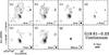 |
Fig. 1 Continuum emission maps toward the G 19.61−0.23 high-mass star-forming region. All the contour levels are drawn with ± 7σ·2n, where σ is the rms noise level of the image (Table 1) and n = 0,1,2,... . The wavelength and FWHM of the synthesized beam are indicated in the bottom right corner of each panel. See Table 1 for the values of the synthesized beams. |
2.4. Combining NMA and OVRO data: the SiO (2–1) v = 0 line
We combined the interferometric SiO (2–1) v = 0 data taken with the NMA (Sect. 2.2) and OVRO (Sect. 2.3) interferometers; the diameters of the element antennas are 10.0 m and 10.4 m, respectively. For this purpose, we adopted the observational set-ups at both interferometers as similar as possible, with two important differences, related to the frequency resolution and the integration time for a single visibility. We therefore smoothed the NMA visibilities every 8 channels, and averaged them to achieve a 3.35-s integration time per visibility. We verified that the visibilities taken with the two arrays were fairly consistent in terms of flux calibration when we compared them over the common range of the projected baseline length. We subsequently produced a 3D cube using the task IMAGR of the AIPS package with a robustness parameter of +1 to find a compromise between angular resolution and image-fidelity.
2.5. SMA observations and data reduction
Aperture synthesis continuum and line emission observations of G 19.61−0.23 at 890 μm were carried out with the SMA on May 12, 2005 in the extended array configuration and on July 8, 2005 in the compact configuration. The shortest projected baseline length, i.e., the shadowing limit, was about 11.9 m. This ensured that our SMA observations were insensitive to structures more extended than 15''̣5, corresponding to 0.95 pc at a distance of 12.6 kpc. The SIS receivers were tuned to a frequency of 335.4158 GHz to observe the 13CO (3−2), C18O (3−2), and CH3CN (18−17) lines in the LSB, and the HC18O+ (4−3) and CN (3−2) lines in the USB. Each side-band covers a 2 GHz bandwidth. The attained synthesized beam sizes, effective velocity resolution after smoothing, and image sensitivity are summarized in Tables 1 and 2.
We used 3C 454.3 as a bandpass calibrator, and J1743–038 and J1924–292 as phase and gain calibrators. The flux densities of the two calibrators were bootstrapped from observations of Uranus and Neptune (J1743−038: 1.64 Jy in May and 1.55 Jy in July; J1924−292: 3.16 Jy in May and 3.60 Jy in July) and stable to within 12% during the observing period. We estimated a final uncertainty in the flux calibration of ~20%. The data calibration was performed using the MIR and MIRIAD packages. Following standard calibration procedures, we tentatively subtracted the continuum emission from the visibility data, then imaged the continuum in each side-band. After verifying that the continuum emission was confined within a compact region at (Δα, Δδ) = (−1''̣2, + 2''̣2) with respect to the phase tracking center (PTC; RA = 18h27m38.15s, Dec = −11°56′39''̣50 in J2000), we subtracted the continuum contribution from the visibility data by providing the position offset to the task UVLIN in MIRIAD package. For the final continuum subtraction process, we identified, at least, 33 and 24 lines in the USB and LSB, respectively. We subsequently constructed continuum emission images with natural and uniform visibility weighting functions in conjunction with the multi-frequency synthesis technique. For the continuum imaging, we did not apply another visibility weighting based on the system temperature (Tsys) of each element antenna, because the Tsys information in the USB for the compact array observations had not been recorded properly. In contrast, the Tsys-based visibility weighting was applied to the line data in the LSB, for which the Tsys was properly recorded.
Atmospheric seeing was estimated using the continuum emission maps of the (point-like) calibrators, because the apparent angular diameter of the calibrators is related to the size scale characterizing the atmospheric turbulence. The time-averaged size scale over each observing track should be comparable to the beam-deconvolved diameters of the calibrators. By this means, we estimated the average seeing for J1743−038 to be 0''̣15 and 0''̣95 for the extended and compact configuration observations, respectively. We found that the seeing towards J1924−292 was twice as poor as that towards J1743−038 in the extended array observations. In addition, given that the angular distance between J1924−292 and the PTC is rather large (21.8°) we decided not to use this quasar as a phase calibrator. We finally reconstructed all the images of the continuum and line emission data.
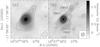 |
Fig. 2 Continuum emission maps at 890 μm taken with SMA toward G 19.61−0.23 with a) natural weighting and b) uniform weighting. The solid contours start at the 3σ level and increase in steps of + 2σ up to the 50% level for a clarity of the maps. The dashed contours start at the −3σ level and decrease in steps of −2σ. The image noise levels are 54.1 and 34.9 mJy beam-1 for panels a) and b), respectively. The sensitivity of the uniformly weighted map is better than that of the naturally weighted map, probably because the visibilities have not been weighted taking into account the system temperature of each antenna (see Sect. 2.5). The synthesized beams are shown in the bottom right corners (1''̣38 × 1''̣22 with PA = −44° for natural weighting; 0''̣85 × 0''̣78 with PA = −32° for uniform weighting). |
Results of submm continuum emission observations.
3. Results and analysis
3.1. Continuum emission
3.1.1. Overview of the G 19.61–0.23 star-forming region
Figure 1 presents the continuum emission maps, including already published 3.8 cm and 3 mm images. As discussed in Paper I, the cm maps, representing free-free emission, show that the region contains a cluster of UC HII regions, i.e., young massive stars. One can see that the overall morphology of the cm emission does not change much with wavelength. Most of the apparent differences are due to the different angular resolutions and sensitivities to extended structures (see Table 1). The 7 mm and 3 mm maps, which have comparable angular resolutions, also exhibits similar structures. This similarity implies that these two images contain both thermal dust emission and optically thin free-free emission, as discussed for the 3 mm map in Paper I. We note that the compact 7 mm emission to the east of UC HII region A (see Paper I for labeling of the UC HII regions) is very likely an artifact caused by inadequate sampling of the visibility plane (Sect. 2.1). The SMA 890 μm image appears to differ significantly from the cm- and mm maps, as it shows a bright compact source towards the HMC position previously reported. No 890 μm sources other than the HMC are detected over the SMA field of view, above a 3σ upper limit of 105 mJy beam-1, corresponding to a brightness temperature in the synthesized beam of Tsb(3σ) = 0.22 K. In the following, we describe the continuum results obtained at 890 μm (Sect. 3.1.2) and the high-resolution images at cm wavelengths (Sect. 3.1.3).
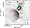 |
Fig. 3 Comparison of the 6 cm (greyscale plus white contour), 3.8 cm (magenta contour), and 1.3 cm (yellow contour) continuum emission maps generated with the common minimum UV distance of 13.3 kλ (see Sect. 3.1.3). Contour intervals for the cm maps and the submm map are the same as those in Figs. 1 and 2, respectively, where the 1σ noise levels are 0.23, 0.18, and 0.36 mJy beam-1 and the beams 0''̣433 × 0''̣321, 0''̣262 × 0''̣195, and 0''̣344 × 0''̣251, for the 6.0, 3.8, and 1.3 cm maps, respectively. The largest of the three beams is shown in the bottom right. The filled red rectangules and the double red circles indicate the peak positions of the 3 mm (Paper I) and 890 μm (Sect. 3.1.2) continuum emission, respectively. The filled green circles and light-blue triangles show the positions of the OH (Garay et al. 1985) and H2O (Hofner & Churchwell 1996) masers, respectively. Labels A and C refer to the UC HII regions (notation as in Paper I and references therein). The filled yellow circle associated with the UC HII region C indicates the peak position of the isolated 7 mm emission seen in Fig. 1e close to the HMC. |
3.1.2. 890 μm continuum emission
In Paper I, we demonstrated that the 3 mm continuum emission towards the HMC is mostly generated by thermal dust emission with a small contribution from free-free emission. The latter is instead insignificant in the newly obtained SMA image at 890 μm, which is dominated by the dust continuum emission. Figure 2 shows a close-up view of the SMA 890 μm images produced with natural and uniform visibility weighting functions. The continuum emission in the natural weighted map (Fig. 2a) is elongated to both the south and northwest. The uniformly weighted map (Fig. 2b) clearly resolves the emission and shows that the elongation can be attributed to two additional weak sources, whose peak intensities are slightly above the 7σ level. These results indicate that there are (at least) three submm sources in the region. Hereafter, we name these SMA1 (the HMC), SMA2 (the core to the south), and SMA3 (the core to the northwest), as indicated in Fig. 2b.
The most intense 890 μm source, SMA1, is located 0''̣32 northeast of the peak of the 3 mm “dust” continuum emission (see Fig. 2c in Paper I and Fig. 3 of this work). This means that the 890 μm and 3 mm continuum peaks coincide within the errors. Therefore, in this study we identify SMA1 with the HMC, whose position is obtained from the 890 μm image (Table 3). The peak intensity (Iν) of the 890 μm continuum emission is 1.89 Jy beam-1, corresponding to Tsb = 31.0 K. The spectral index (α) between 3 mm and 890 μm is α3 mm − 890 μm ≳ 2.7, implying a power-law exponent for the dust emissivity, β, of ≳ 0.7, assuming optically thin dust emission and the Rayleigh-Jeans approximation. For this estimate, we integrated the 890 μm flux over the three sources SMA1, SMA2, and SMA3 and used the continuum flux at 3 mm (147 mJy) obtained from the data of Paper I, where the free-free continuum contribution from the nearby UC HII region was subtracted by extrapolating the 1.3 cm continuum map to 3 mm based on the assumption of optically thin emission. We emphasize that the latter flux is affected by significant uncertainties due to the method adopted to subtract the free-free contribution (see Paper I). Therefore, in the following we prefer to adopt β = 1, which is consistent with the value derived above, within the uncertainty, and falls in the range β = 1−2 found in the literature.
The 890 μm flux densities (Sν) in Table 3 allow us to estimate the gas-plus-dust mass traced by thermal emission (Mdust). For this purpose, we assumed a dust temperature (Tdust) of 80 K (Paper I) and calculated the values of Sν by integrating the emission in Fig. 2b over the regions inside the 5σ contour levels of the sources. The value Tdust ≃ 80 K was obtained from the fit to the continuum spectrum (see Paper I), from the cm to the mid-infrared regime, including the newly obtained 7 mm and 890 μm fluxes. We estimate that the ambiguity in defining the boundary between SMA1 and SMA2 causes a ~5% error in the value of Sν. The resulting masses are given in Table 3. We note that these values are approximately inversely proportional to the dust temperature and are thus affected by the uncertainty in this latter parameter accordingly. Since the assumed temperature is most likely to be correct to within a factor 2, we assume that the estimated masses are also affected by a similar uncertainty.
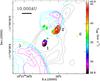 |
Fig. 4 First moment map of the H2O masers (color image) and maps of the continuum emission (color contours). The black contours overlayed on the maser velocity map correspond to the integrated intensity of the maser spots, with levels starting from the 5σ level with 5σ steps. The black, cyan, and magenta contours represent the first 3 contours of the 890 μm, 6 cm, and 3.8 cm continuum emission, respectively (the same as in Fig. 2). The yellow triangles and green-filled circles show, respectively, the positions of the H2O (Hofner & Churchwell 1996) and OH (Garay et al. 1985) masers. The numbers associated with the yellow triangles are used to identify the maser features as done by Hofner & Churchwell (1996). |
3.1.3. Centimeter continuum emission towards the HMC
To assess whether cm emission is present at the position of the HMC, we reconstructed the VLA 6 cm, 3.8 cm, and 1.3 cm continuum images in Fig. 3 by making use of visibilities whose minimum spatial frequency is set to be the same for the 3 bands. We chose the shortest baseline equal to 13.3 kλ, namely that of the 890 μm maps (see Table 1). This allows one to resolve out the extended emission. Figure 3 clearly shows that no free-free emission is detected towards the peak positions of the three 890 μm sources. We note that SMA1 is located at the center of the H2O and OH masers’ distributions, whereas no H2O and OH maser spot appears to be associated with SMA2 and SMA3. The upper limits (3σ) obtained from the cm images correspond to brightness temperatures over the synthesized beam (Tsb) of 199, 230, and 30.9 K, respectively at 4.86, 8.42, and 22.27 GHz (see the caption of Fig. 3 for the corresponding noise levels and beam sizes).
We point out that the 7 mm emission seen to the north of the HMC (see Fig. 1e) coincides with the cometary UC HII region C (Fig. 3). We thus argue that free-free emission from this UC HII region should significantly contribute to the corresponding 7 mm continuum emission, whose peak intensity is 25.3 mJy beam-1 (~10σ). We also note that SMA3 lies right in front of the vertex of the cometary shaped UC HII region C, suggesting a physical connection between the two. This could explain the cometary-shape, with the existence of dense material preventing expansion of the ionized gas towards the northwest.
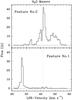 |
Fig. 5 H2O maser spectra toward the maser features Nos. 1 and 2 obtained by integrating the emission inside the 5σ contour of each emission (see Fig. 4). The vertical dashed line indicates the systemic velocity (Vsys) of the cloud, VLSR = 41.6 km s-1. |
3.2. H2O masers
3.2.1. Overall results
Figure 4 compares the H2O maser distribution with that of the UC HII regions. The color image is a map of the first-order moment of the maser lines. We detected two out of the six “maser features” previously reported by HC96, i.e. features N. 1 and 2 in their notation. Here, we use the term “maser feature” to describe a well-defined, spatially isolated group of maser spots (see, e.g., HC96 and Furuya et al. 2005b). With an angular resolution of 0''̣3, one cannot distinguish the maser spots associated with all the different lines seen in the spectrum (Fig. 5). We argue that the high variability of H2O masers maybe the reason why no maser emission was detected towards the other four features identified by HC96. This is because the intensities measured by HC96 are all well above our 3σ sensitivity of 135 mJy beam-1.
Figures 4 and 5 clearly show that feature 1 exhibits only blueshifted emission, whereas feature 2 is mostly redshifted, despite the presence of a few blueshifted lines. Notwithstanding the well known substantial variability of water masers, we note that these two features have persisted with approximately the same spectral shape since December 1991, when the VLA observations of HC96 were carried out. The terminal velocities (Vt) at which blue- and red-shifted maser emissions are seen towards features 1 and 2 differ by ~15−20 km s-1 with respect to the systemic velocity (Vsys) of 41.6 km s-1. All this suggests that the maser emission may be originating in a bipolar jet driven by a putative young stellar object (YSO) inside the HMC. We return to this issue in Sect. 3.3.4.
3.2.2. Origin of the H2O maser features 1 and 2
Features 1 and 2 (see Figs. 4 and 5) seem to have persisted for more than a decade. From their distribution (see Fig. 3 of HC96), one can argue that only these two features of the six reported by HC96 are associated with SMA1.
Interferometric observations of H2O masers at 22 GHz indicate that they are probably excited in shocked regions at the interface between (proto)stellar jets and the ambient gas (e.g., Furuya et al. 2000), although in some objects these masers have been suggested to be tracing rotating disks (e.g., Torrelles et al. 1996). If the latter were the case for the masers in SMA1, one could infer the mass needed to ensure centrifugal equilibrium from the separation between the blue- and red-shifted features (1''̣70) and their relative velocities (~35 km s-1). We obtain ~3700 M⊙, which is ~3 times greater than that obtained from the submm continuum emission (see Table 3). This suggests that rotation is not a viable description of the kinematics of the masers in the HMC. Moreover, as we see in Sect. 3.3.4, the H13CO+(1−0) line appears to trace a bipolar outflow oriented SE−NW. In this scenario, the two H2O maser features may be associated with a bipolar jet feeding the outflow. We thus conclude that the jet interpretation is more likely.
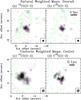 |
Fig. 6 Total integrated intensity maps of the 13CO (3−2) (left panels) and C18O (3−2) (right panels) lines produced with natural (upper panels) and uniform (lower panels) visibility weighting functions. Note that the upper panels show the whole area of the G 19.61−0.23 star-forming region, while the lower panels magnify the region centered on the HMC (greyscale plus thin contour; see Table 2). For comparison purposes, the 7σ level contour of the 6 cm continuum (i.e., free-free) emission as in Fig. 1a is shown by thin green contours. The magenta stars indicate the peak positions of the three 890 μm continuum sources (Table 3). The contours of the CO isotopomer maps start from the 5σ level in steps of 3σ, where the 1σ noise levels are 1.9 and 1.8 Jy beam-1 km s-1 for the natural and uniform weighted 13CO maps, and 0.8 Jy and 1.7 beam-1 km s-1 for the natural and uniform weighted C18O maps, respectively. We integrated the emission over the LSR-velocity ranges 30.2 ≤ VLSR/km s-1 ≤ 42.2 for 13CO, and 34.7 ≤ VLSR/km s-1 ≤ 44.5 for C18O. All the other symbols are the same as those in Fig. 1. The emission seen in the top of the upper-panels is an artifact caused in the cleaning process. |
3.3. 13CO (3–2), C18O (3–2), H13CO+ (1–0) and SiO (2–1) line emission
3.3.1. Maps of 13CO (3–2) and C18O (3–2) line emission
Figure 6 presents total integrated intensity maps of the 13CO and C18O J = 3−2 lines produced using natural and uniform weightings. For the sake of comparison, we plot the 7σ contour level of the 6 cm continuum emission map, i.e. the lowest level from Fig. 1. The natural weighted maps show that the 13CO and C18O (3−2) emitting regions are compact and centered on the HMC, while these lines are not detected towards SMA3. Since single-dish observations of similar objects generally indicate that these CO isotopomers trace extended regions, it is reasonable to argue that in G 19.61−0.23 the extended emission is filtered out by the interferometer. We also note that the 13CO and C18O (3−2) lines are not seen towards SMA1 in the uniform weighted maps.
3.3.2. Spectra at the peak position of the HMC
Figure 7 shows the molecular line spectra obtained from the interferometric observations towards the peak position of SMA1. The H13CO+ line peaks at Vsys, but its line profile is not a single Gaussian. The SiO line shows prominent high velocity wing emission. Noticeably, the 13CO (3−2) and C18O (3−2) lines do not show prominent wing emission, but exhibit deep absorption features. In both CO isotopomers, redshifted absorption (i.e. an inverse P-Cygni profile) is seen, albeit fainter in the C18O line. The straightforward interpretation of these finding is that the HMC is undergoing infall. The LSR-velocity of the deepest absorption channel is VLSR = 44.5 km s-1 for 13CO, and 46.0 km s-1 for C18O, the latter being redshifted by 4.4 km s-1 with respect to Vsys. The deepest absorption channels of the 13CO and C18O lines have −29.3 K and −15.0 K in Tsb, respectively. We note that the brightness temperature of the 13CO line (and even more so for the C18O line) is, in absolute value, less than that of the continuum peak (see Sect. 3.1.2); this indicates that the absorption line is real and not an artifact due to resolving out the extended emission.
Finally, we note that we cannot exclude that a part of the blueshifted wing emission of the 13CO (3−2) line might be related to the CH CN K = 7 line, as we argue in Sect. 3.4. After considering all the other molecular lines that could overlap with the two CO isotopomer lines, we conclude that 13CO line over the velocity range between VLSR ~ 34 km s-1 and 50 km s-1, and the C18O between ~0 km s-1 and 65 km s-1 are free from line contaminations.
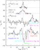 |
Fig. 7 Spectra of four molecular lines in Tsb scale towards the peak of the 890 μm continuum emission, i.e., SMA1. The SiO and H13CO+ intensities are scaled by a factor 2.0. The vertical dashed line indicates the systemic velocity (Vsys) of the cloud, VLSR = 41.6 km s-1. In the CO isotopomers spectra, we mark the positions of all possible (molecular) lines, calculated assuming that they are emitted with velocity equal to Vsys (see Sect. 3.3.2). The thick horizontal blue and red bars denote the velocity intervals over which the line emission has been integrated to produce the maps in Figs. 9, 10, and 16. The emission seen around VLSR ≃ 70 km s-1 of the C18O spectrum probably originates in the HNCO line rather than CH |
3.3.3. Comparisons of the absorption features seen in the 13CO (3–2) and HCO+ (1–0) Lines
To assess the origin of the redshifted absorption seen in the 13CO and C18O (3−2) spectra, in Fig. 8, we compare the 13CO(3−2) spectrum with an HCO+ (1−0) spectrum taken with the IRAM 30 m telescope (R. Cesaroni, unpublished data). The HCO+ spectrum shows a number of prominent absorption features. To ensure that the comparison is as consistent as possible, we reconstructed the 13CO image from the visibility data adopting the same beam as the HCO+ line (θHPBW = 29″). We then took the 13CO spectrum towards the same position observed in the HCO+ line. We note that all the absorption features seen in the two lines are redshifted with respect to Vsys. However, absorption is detected at different velocities in the two tracers: the absorption dips are seen at VLSR − Vsys = +3.5 km s-1 for 13CO, and at VLSR − Vsys ≃ +10, +29, and +57 km s-1 for HCO+. We assume that the two features seen at the highest velocities in HCO+ are produced by clouds along the line-of-sight, because their velocities correspond to those of the 21 cm HI lines observed by Kolpak et al. (2003) (see their Fig. 4). This suggests that all the HCO+ absorption most likely occurs against the UC HII regions in G 19.61−0.23. In contrast, no HCO+ absorption is detected in the velocity range where 13CO and C18O absorption is seen, implying that the latter is caused by the HMC, i.e. has a local origin, and thus indicates that the core is experiencing infall. The nature of the absorption will be discussed further in Sect. 4.2.1, where we study the gas infall in the core.
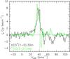 |
Fig. 8 Comparison of the absorption features seen in the 13CO (3−2) and HCO+ (1−0) lines toward the peak of the 890 μm continuum emission. For the sake of comparison, the interferometric 13CO (3−2) spectrum has been obtained after reconstructing the data with a synthesized beam equal to the single-dish beam of the HCO+ line observations with IRAM 30-m telescope (see Sect. 3.3.3). |
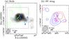 |
Fig. 9 a) Integrated intensity map of the H13CO+ (1−0) bulk emission. The velocity range used for the integration is 35.5 ≤ VLSR/km s-1 ≤ 48.9. The interval between the thin-black contours is 2σ with the lowest contour corresponding to the 3σ level, where the 1σ rms noise is 0.53 Jy beam-1 km s-1. The thin-white contours are the 95% and 90% levels of the corresponding peak intensities, where the 90% levels correspond to the 7.5σ level. All the other symbols are the same as those in Fig. 6, and the numbers associated with the three maser spots to the west are the same as those used by Hofner & Churchwell (1996). The dashed box indicates the area shown in the right-hand panel. b) Overlay of the blue- and redshifted wing emission maps of the H13CO+ (1−0) emission. The contours are 2σ steps starting from the 3σ level. The blue- and redshifted wing emission maps were obtained by averaging the wing emission over the intervals 35.3 < VLSR/km s-1 < 37.9 and 43.1 < VLSR/km s-1 < 49.2, and their rms noise levels are 43.8 and 30.2 mJy beam-1, respectively. |
3.3.4. H13CO+ (1–0) emission
Here, we present the results of the H13CO+ (1−0) line observations performed with the OVRO array (Table 2). Figure 9 presents maps of both the bulk and line wing emission. One can see that, while the former outlines a structure elongated approximately NE−SW, the latter can be interpreted as a bipolar outflow oriented SE−NW.
Comparison with the positions of the three submm continuum sources shows that SMA1 is the closest to the geometrical center of the outflow, hence is the most likely candidate object for driving it. Here the geometrical center is defined as the middle point on the line connecting the peaks of the blue- and redshifted lobes. We obtain (projected) angular distances to the center of 3''̣2, for SMA1, and 3''̣8, for SMA2. That SMA1 is at the origin of the flow is also supported by comparison with the H2O maser jet associated with SMA1, discussed in Sect. 3.2. This jet is also oriented parallel to the H13CO+ outflow and has the same red–blue symmetry, which strongly suggests a common origin for the two.
Using the bulk emission map, we estimated the H13CO+ abundance relative to H2 (XH13CO + ) from the ratio between the mean H13CO+ column density over the 3σ contour level of the 890 μm continuum emission (see Fig. 9a) and the corresponding H2 column density obtained from the submm continuum emission. This estimate is very sensitive to the temperature of the gas and dust. In our calculation, we assumed that the gas and dust are well-coupled, thus having identical excitation and dust temperatures. For a fiducial value of 80 K (Sect. 3.1.2), we obtained an abundance of ~10-10, but one should keep in mind that XH13CO + spans a range from ~3 × 10-11 to ~6 × 10⁻¹⁰ for T varying by a factor 2 with respect to the fiducial value.
Assuming XH13CO + = 10-10 and T = 80 K (Sect. 3.1.2), we computed the outflow parameters by integrating the line emission for the blue and red wings (see caption of Fig. 9 for their velocity ranges). With these assumptions, we obtained a total outflow mass (Mlobe) of 3700 M⊙ and a momentum of 14 000 M⊙ km s-1. we note that, even ignoring the error in XH13CO + , a factor 2 uncertainty in the gas temperature affects by an additional factor ~2 the outflow parameters. The dynamical timescale (td) is estimated from the ratio of the maximum extent of the lobes to the difference (in absolute value) between the systemic velocity and the terminal wing velocity. We obtain ~8 × 10⁴ yr, without correcting for the (unknown) outflow inclination. The mass-loss rate (Ṁflow) and a momentum rate (Fflow) are thus 0.05 M⊙ yr-1 and 0.17 M⊙ km s-1 yr-1, respectively. Values that large are very likely overestimated because of the various assumptions made. Nevertheless, they indicate that the powering source should be as luminous as ~105 L⊙, according to the empirical relationship derived by Beuther et al. (2002). To obtain these values, we implicitly assumed that one is dealing with a single star. If this is correct, then the putative star must be in a pre-HII region phase, as no free-free continuum emission has been detected towards the HMC. We discuss this further in Sects. 4.1 and 4.3.
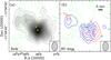 |
Fig. 10 a) Integrated intensity map of the bulk emission of the SiO (2−1) v = 0 line (greyscale plus thin contours) observed with the OVRO and NMA interferometers. The green contours have the same meaning as in Fig. 6. The bulk emission has been integrated over the LSR-velocity range of 31.9 ≤ VLSR/km s-1 ≤ 48.4, and the rms noise level is 0.28 Jy beam-1 km s-1. The yellow stars represent the positions of SMA1, SMA2, and SMA3 (see Table 3). b) Overlay of the blue- and redshifted wing emission maps of the SiO (2−1) v = 0 emission. The contours are spaced by 2σ and start at the 3σ level. The blue- and redshifted wing emission maps have been obtained by averaging the wing emission over the intervals 21.1 < VLSR/km s-1 < 31.9 and 48.4 < VLSR/km s-1 < 58.0, and their rms noise levels are 11.6 and 13.9 mJy beam-1, respectively. The hatched ellipses in the bottom right indicates the FWHM of the synthesized beam (Table 2). |
3.3.5. SiO (2–1) v = 0 emission
Maps of the SiO emission –
from Fig. 7, one can infer that the Vt of the SiO emission is blueshifted by ~11 km s-1 and redshifted by ~15 km s-1 with respect to Vsys. The detection of HV wing emission is strongly indicative of the presence of a molecular outflow driven by a YSO in one of the cores. To analyze the structure of the SiO emitting gas, we produced maps of the bulk emission and HV wing emission in Fig. 10. In panel (b), one sees that the HV wing emission is elongated along the east-west direction, with the blue lobe being aligned towards the east and the red lobe to the west. This bipolarity indicates that the SiO HV gas very likely traces a bipolar outflow, although the lobes do not appear to be very collimated. Since the two lobes are largely overlapping each other, the outflow is most likely to be close to pole-on. Interestingly, the velocity structure of the SiO outflow is very different from that of the larger scale (~20″) 13CO (2−1) outflow mapped by Loṕez-Sepulcre et al. (2009) with the IRAM 30-m telescope. The latter has the redshifted lobe to the NE and the blueshifted one to the SW. We emphasize that this is not due to the different velocity intervals used to produce the outflow maps, because the orientation of the SiO outflow does not change using the same velocity ranges adopted by Loṕez-Sepulcre et al. (narrower than those used by us). We conclude that in all likelihood the larger scale flow is originating in another YSO in the region.
What is the source powering the SiO outflow? We conclude that it is SMA2, despite the small offset between this and the geometrical center of the outflow (see Fig. 10b), because Fig. 10a shows that the peak of the SiO bulk emission is clearly coincident with SMA2 (see Fig. 10a).
We note that this implies that (at least) three bipolar outflows are present in the region. Besides the large-scale flow mapped by Loṕez-Sepulcre et al., we detected two compact outflows: one traced by H13CO+ (see Sect. 3.3.4) and powered by a YSO in SMA1, and another traced by SiO and powered by a YSO embedded in SMA2. Is the latter as massive as the former? We now present an estimate of the YSO luminosity from the SiO outflow parameters.
Properties of the SiO outflow driven by SMA2 –
to derive the mass and kinematical parameters of the outflow, we assume that the SiO line is optically thin and the SiO molecule is in LTE. We adopt an excitation temperature (Tex) of 20 K (Appendix A) and an SiO/H2 abundance ratio of 3 × 10⁻⁹. The latter is estimated from the ratio of the SiO column density (obtained from the bulk emission – Fig. 10a) to the H2 column density (calculated from the 890 μm continuum emission towards SMA 2 – Table 1). We note that that the outflow masses are most likely underestimated because of missing flux filtered out by our interferometric observations and the uncertainty in defining a boundary velocity (Vb) between the outflowing gas and the quiescent ambient gas.
We measured an outflow mass of 90 M⊙ and a momentum of 2100 M⊙ km s-1. We also obtained td ≃ 2 × 10⁴ years, implying an outflow mass-loss rate Ṁflow ≃ 5 × 10⁻³ M⊙ yr-1 and a momentum rate Fflow ≃ 0.06 M⊙ km s-1 yr-1. Since outflows are thought to be momentum driven (Cabrit & Bertout 1992), the latter value may be taken as an indicator of the outflow strength and hence of the mass and luminosity of the YSO powering it. Using the relationship between Fflow and YSO luminosity obtained by Beuther et al. (2002), we found that the YSO powering the SiO outflow should be as luminous as ~3 × 10⁴ L⊙. This indicates that the powering source is a high-mass star.
When deriving the outflow parameters as here for SiO and in Sect. 3.3.4 for H13CO+, a word of caution is required. The difference between the masses of the H13CO+ outflow driven by SMA1 and the SiO outflow from SMA2 amounts to a factor ~40. This large number may be due to multiple outflows unresolved in our observations as well as the uncertainties in the fractional abundances of the two molecules, which are difficult to predict. These caveats cast some doubt on the values derived in our calculations. Therefore, although the basic conclusion that the two outflows are associated with high-mass YSOs is likely to be correct, the outflow parameters reported here must be considered with caution.
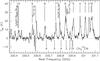 |
Fig. 11 Interferometric spectrum of the CH3CN and CH313CN (18−17) lines towards the peak position of the 890 μm continuum source, SMA1. The vertical bars above and below the spectrum indicate the rest-frequencies of the K components of the CH3CN and CH313CN J = 18−17 transitions. We also indicate other lines that may be blended with the methyl cyanide lines. |
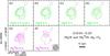 |
Fig. 12 Integrated intensity maps of the JK = 18K − 17K emission of the CH3CN (green contour) and CH313CN (magenta contour) lines. The black dashed contour corresponds to the absorptions region seen in the 13CO (3−2) line. The thin black contour represents the 7σ level of the uniform weighting 890 μm continuum emission map (Fig. 2b). All the transitions, except the CH3CN K = 0, 1, and 2 components, are not blended with other lines (see Fig. 11 for the spectrum). The contour intervals are spaced by 2σ and start from the 3σ level. In the CH3CN maps, we do not plot contours above the 17σ level to prevent saturation of the maps. The 1σ rms noise levels are 6.3, 1.4, 1.3, 0.33, and 0.17 mJy beam-1 km s-1 for the CH3CN (18−17) K = 0 to 2 emission, K = 3, K = 4, and CH313CN (18−17) K = 2, and K = 6, respectively. |
3.4. CH3CN 18K − 17K emission
3.4.1. Spectrum
Figure 11 shows the spectrum of the CH3CN and CHCN JK = 18K − 17K lines observed with the SMA towards the 890 μm continuum peak, SMA1 (Sect. 3.1.2). High-excitation K components can be seen in this spectrum. In particular, one can recognize all lines up to K = 10 for CH3CN, and all up to K = 6 for CHCN, although overlap with transitions from other species (some of which are marked in the figure) cannot be excluded. Only the components of CH3CN (18−17) K = 3 and K = 4 and CHCN (18−17) K = 2 and 6 do not appear to be affected by blending.
The peak intensities of the K = 0 to 4 lines of the CH3CN are comparable to each other, suggesting that these CH3CN lines are optically thick. One can calculate the optical depth (τ) of the corresponding CHCN lines from the ratio of the two isotopomers. The values of τ for the 13C substituted species range from 0.1 to 0.5 for K ≤ 5. These imply optical depths of 5 to 29 for CH3CN, assuming a 12C/13C abundance ratio of 55 at a galactocentric distance of 5.3 kpc (Wilson & Rood 1994). As we will discuss in Sect. 3.4.3, opacities that large hinder the usage of rotation diagrams to estimate the gas temperature and column density.
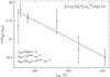 |
Fig. 13 Rotation diagram obtained from the K = 0, 1, 2, 4, 5, and 6 components of the CH |
3.4.2. Maps: comparison with the other lines
Figure 12 shows maps of some CH3CN and CH313CN (18−17) lines that are not blended with transitions of other molecules. For the sake of comparison, we also outline in the same figure the uniform weighted 890 μm continuum map (Fig. 2b) and map of the redshifted absorption seen in the 13CO (3−2) emission, described in Sect. 3.3.2. The 13CO (3−2) map corresponds to the velocity channel where the maximum absorption is attained, i.e., at VLSR = 44.0 km s-1. We recall that no emission is seen towards SMA1 in the integrated intensity maps of the 13CO and C18O (3−2) lines (Fig. 6). From all this, one obtains the following results: (i) CH3CN and CHCN line emission is detected towards SMA1 and SMA2, but not towards SMA3; (ii) the peak of the methyl cyanide emission coincides with the peak of SMA1; (iii) the redshifted 13CO absorption is seen towards the center of the HMC (i.e., SMA1), but is not detected towards SMA2 and SMA3; (iv) the emitting region of the low K-transition, e.g., K = 0, 1, and 2, has a size similar to that of the the higher K-lines, while in similar objects (e.g., Beltrán et al. 2004) the emitting region is smaller for higher excitation transitions.
3.4.3. Excitation conditions of CH3CN
Methyl cyanide is known to be an excellent temperature tracer, and rotation diagrams derived from the different K components are commonly used to estimate the gas temperature and column density. However, as argued in Sect. 3.4.1, most CH3CN (18−17) transitions are optically thick, thus making the column density at the corresponding level a lower limit. To circumvent this problem, we used the optically thin (τ < 0.5 – see Sect. 3.4.1) lines of CHCN. Despite heavy blending with other transitions, we managed to obtain an estimate of the line parameters by fitting groups of K components simultaneously, by fixing their separation in frequency to the laboratory values and forcing the line widths to be the same. In this way, we were able to successfully fit the K = 0,1,2,4,5, and 6 components and produce the rotation diagram shown in Fig. 13. In our calculation, we assumed a source angular diameter of 2''̣4 from Table 3 and a 12C/13C abundance ratio of 55. The best-fit solution infers a temperature of 208 ± 41 K and a source averaged CH3CN column density of 2.7 × 1016 cm-2. While the latter is consistent with the values quoted by Wu et al. (2009) and Qin et al. (2010), the former is significantly lower than their estimates of 552 ± 29 K (Wu et al. 2009) and 609 ± 77 K (Qin et al. 2010). This discrepancy is caused by these authors use the optically thick CH3CN lines in their calculations, which leads to a severe overestimate of the true rotation temperature.
Since the source angular diameter is comparable to the SMA beam and the CH3CN line are optically thick, the line brightness temperature should be similar to the gas kinetic temperature of ~200 K. Instead, only ~20 K is measured with the SMA (see Fig. 11), implying a beam filling factor of 0.1. Although sub-structures due to clumpiness on angular scales smaller than the interferometer beam are very likely, this filling factor appears to be too small, as we do not reveal possible fragmentation of the HMC in our maps. We thus believe that beam dilution may explain only in part the low value of Tsb and conclude that the optically thick CH3CN lines must be tracing the outer regions of the core, where the gas temperature is significantly less than the temperature measured in the thinner CHCN transitions because it originates in the innermost regions.
3.4.4. Velocity structure of the HMC traced by CH3CN emission
To investigate the velocity field of the innermost part of the SMA1 core, in Fig. 14, we plot maps of the CH3CN line centroid velocity over the HMC. This velocity field was obtained by fitting simultaneously multiple K-components with Gaussian profiles with separations in frequency fixed to the laboratory values (see Pearson & Mueller 1996) and line widths forced to be equal. The method employed here is described in e.g., Beltrán et al. (2005) and Furuya et al. (2008). Considering the line-blending and high opacity at low-K lines of CH3CN (Sect. 3.4.1), we decided to fit the CH3CN K = 7 and CHCN K = 5 lines simultaneously, to obtain the map in Fig. 14a, and the CH3CN K = 8 and CHCN K = 6 lines, for the map in Fig. 14b. The values of the velocity are displayed only inside the area encompassed by the 9σ contour level of the corresponding integrated emission map.
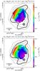 |
Fig. 14 Maps of the line peak velocity (color) obtained from simultaneous Gaussian fits to the CH3CN and/or CH |
Unlike other cases (Beuther et al. 2005), the CH3CN lines in our study appear to trace a clear velocity gradient, increasing from SW to NE, as observed in similar sources (e.g. Beltrán et al. 2004). In the G 19.61−0.23 HMC, the inferred velocity field maps show a coherent pattern that is indicative of systematic motions in the gas. In addition, the two maps are in fairly good agreement. To confirm these findings, we produced velocity-field maps by fitting a single-Gaussian profile to the weak, optically thin CHCN K = 2 component, which is not blended with other transitions. In this case, the velocity map also confirms the existence of a velocity gradient and demonstrates that this is not due to opacity effects.
We note that the velocity gradient is almost perpendicular to the axis of the H2O maser jet in Fig. 4 and that of the H13CO+ outflow in Fig. 9b. Therefore, our explanation of the velocity gradient is that the HMC is rotating about the jet/outflow axis oriented SE−NW, alike the “toroids” imaged by Beltrán et al. (2006).
4. Discussion
4.1. Evolutionary stage of the massive YSOs in the 3 submm sources
Previous studies (e.g., Codella et al. 1997) have shown that H2O masers are preferentially coincident with dense molecular cores that do not display continuum emission from ionizing gas, implying that these cores may harbor massive YSOs detected prior to the formation of an HII region. This is also consistent with the case of low- and intermediate mass stars, where H2O masers are known to be associated with the youngest evolutionary phases (Furuya et al. 2001, 2006). Given the high masses of the three submm cores in G 19.61−0.23 – on the order of 101−103 M⊙ – one can hypothesize that each of them could develop an HII region; that, instead, no free-free emission is detected inside the cores (Sect. 3.1.3), as well as the presence of a H2O masers jet in SMA1 (Sect. 3.2), suggest that the YSOs harbored in the cores are massive but in an early evolutionary stage.
It is possible to constrain the properties of the putative HII regions and corresponding ionizing stars embedded in the cores using the upper limits obtained from our observations of the continuum emission. For this purpose, we use the method illustrated by Codella et al. (1997) (see also Molinari et al. 2000).
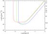 |
Fig. 15 Plot of the brightness temperature in the synthesized beam of a Strömgren HII region, as a function of radius and Lyman continuum photon rate (see Sect. 4.1 for details). The curves correspond to the 3σ upper limits on the free-free continuum emission measured towards SMA1 at 4.86 GHz (blue), 8.42 GHz (green), and 22.273 GHz (red). Here the rms noise levels and the geometrical mean of the beam FWHPs adopted to plot are 230 μJy beam-1 at 5 GHz, 180 μJy beam-1 at 8 GHz, and 360 μJy beam-1 at 22 GHz. The labels to the right indicate the spectral types of the ZAMS stars with the corresponding value of NLy, according to Panagia (1973). |
For the sake of simplicity, we arbitrarily assume that each submm source develops a single massive YSO, instead of a cluster. As explained in Codella et al. (1997), the peak brightness temperature, Tsb, of a Strömgren HII region at a given frequency can be expressed as a function of the radius, Rs, and Lyman continuum photon rate, NLy, of the star. In the calculation, we also adopted a source distance of 12.6 kpc, and an electron temperature (Te) of 7200 K, corresponding to the mean for the UC HII regions in G 19.61−0.23 (Garay et al. 1998). For a given Tsb, one obtains a curve like those plotted in Fig. 15. We note that we have not considered the 7 mm image (Sect. 3.1.3), because this has resolution and sensitivity about 3−5 times worse than the cm images. The three curves correspond to 3σ upper limits obtained from the VLA continuum maps at 1.3, 3.8, and 6 cm. The permitted values of Tsb are those lying under each curve. An additional constraint is set by the maximum radius of the HII region, which cannot be larger than the core radius, namely 0.025−0.072 pc, depending on the core (Table 3).
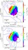 |
Fig. 16 The color maps are the same as in Fig. 14, while the superimposed solid blue and dashed red contours represent, respectively, the blueshifted emission and redshifted absorption seen in the 13CO (left panel) and C18O (right panel). To obtain these plots, we integrated the line over 3 velocity channels centered on the deepest absorption and the most intense emission, namely over the ranges: 34.2 ≤ VLSR/km s-1 ≤ 35.8 for the blueshifted 13CO emission, 43.8 ≤ VLSR/km s-1 ≤ 45.0 for the redshifted 13CO absorption, and 36.0 ≤ VLSR/km s-1 ≤ 38.4 for the blueshifted C18O emission, 44.0 ≤ VLSR/km s-1 ≤ 46.4 for the redshifted C18O absorption. These velocity ranges are outlined by the horizontal blue and red bars in Fig. 7. All the contours are in steps of ± 2σ and start from the ± 3σ level. The stars mark the peak positions of SMA1 and SMA2. See Sect. 4.2 for details. |
If the putative embedded stars are massive, i.e. earlier than approximately B0.5, they must be also very young, as the corresponding HII regions cannot be larger than 6 × 10⁻⁴ pc = 130 AU, which means that they are basically quenched. On the other hand, we cannot rule out the possibility that the stars are later than B0.5, and in this case the HII regions could be larger and optically thin. We conclude, however, that the latter possibility is less likely given the above-mentioned high masses of the cores and the signposts of high-mass star formation associated especially with SMA1 (i.e. water masers, high temperature, and high-excitation lines), and thus conclude that in all likelihood the HMC hides OB type stars in a pre-UC HII region phase.
4.2. Velocity structure of the SMA1 core: infall plus rotation
The velocity structure seen in CH3CN, a high-density, high-temperature tracer, is very different from that obtained from the 13CO and C18O (3−2) lines (see Fig. 16). A comparison between the blue- and red-shifted emission in these lines and the velocity field of the CH3CN transition is shown in Fig. 16. The most interesting result is that both the deepest absorption and the 890 μm continuum peak coincide with the center of symmetry (both in space and velocity) of the CH3CN distribution. This configuration provides a strong indication that HMC is both rotating about a SE−NW axis and collapsing. That no hint of infall, i.e. no redshifted (self)absorption is detected in the CH3CN lines can be explained by these being higher-energy transitions than the 13CO and C18O (3−2) lines. The absorption observed in the latter very likely arises in the outer, low-density regions of the core where the temperature is significantly less than that of the high-density gas traced by CH3CN. In the following, we discuss the details of this scenario and derive some physical parameters characterizing the infalling/rotating gas.
4.2.1. Infall
The negative features observed in the 13CO and C18O (3−2) spectra relate to absorption against the innermost, optically thick part of the core. Unlike the case of absorption at cm wavelengths, where the outer regions of a molecular envelope absorb the free-free continuum of an embedded HII region, here we have detected absorption against the continuum emitted by the core itself. The problem is thus complicated by the gas and dust being mixed, such that both line and continuum photons are emitted from any point inside the core. However, in the outer regions of the core (where absorption occurs) the density is probably low enough to decouple the line radiative transfer from that in the continuum, whereas in the innermost region (where the bright continuum emission originates) the dust optical depth is large enough to absorb all line photons. With this in mind, we can simplify the problem by assuming a spherical core consisting two regions: an outer molecular shell enshrouding an inner, optically thick dusty nucleus. The temperature increases outside-in, so that the nucleus is hotter than the shell. In this configuration, the line brightness temperature measured along the line of sight through the center of the core can be written as ![Mathematical equation: \begin{equation} T_{\rm B} = [J_\nu(T_{\rm ex})-T_{\rm c}] (1-{\rm e}^{-\tau}), \label{eq:rt_abs} \end{equation}](/articles/aa/full_html/2011/01/aa14402-10/aa14402-10-eq155.png) (1)where Tc ≃ 31 K (Sect. 3.1.2) is the measured continuum brightness temperature, τ is the line optical depth, and Jν is defined as Jν(T) = hν/ { k [exp(hν/kT) − 1] } , with h and k Planck and Boltzmann constants, respectively. We neglected the contribution of the cosmological background temperature (TBG ≃ 2.7 K), because this is very small at the 13CO and C18O (3−2) line frequencies (hν/k ≃ 15.9 K, hence Jν(TBG) ≃ 0.045 K).
(1)where Tc ≃ 31 K (Sect. 3.1.2) is the measured continuum brightness temperature, τ is the line optical depth, and Jν is defined as Jν(T) = hν/ { k [exp(hν/kT) − 1] } , with h and k Planck and Boltzmann constants, respectively. We neglected the contribution of the cosmological background temperature (TBG ≃ 2.7 K), because this is very small at the 13CO and C18O (3−2) line frequencies (hν/k ≃ 15.9 K, hence Jν(TBG) ≃ 0.045 K).
Equation (1) can be written for both the 13CO and the C18O (3−2) lines, taking into account that the values of TB are −29 K and −15 K, respectively, and τ(13CO) = 6.4 τ(C18O). From the two equations, one obtains τ(13CO) ≃ 4.5 and Tex ≃ 7 K. For a line width of ~6 km s-1, these imply a 13CO column density of ~1.8 × 1017 cm-2 and an H2 column density NH2 ≃ 1023 cm-2, assuming a 13CO abundance of 1.5 × 10⁻⁶.
Such a low value of Tex is inconsistent with the absorbing gas being associated with the HMC and suggests that absorption could be due to a cold layer of molecular gas located in the outer regions of the cloud. Alternatively, the absorbing gas could cover only a fraction of the continuum. In this case, one must introduce a filling factor < 1 multiplying Jν(Tex) in Eq. (1) and the value of 7 K becomes a lower limit.
Assuming that the absorbing gas is indeed associated with the HMC, one can roughly estimate the mass accretion rate for a constant density distribution 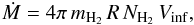 (2)where we assume that the infall speed (Vinf ≃ 4 km s-1) is equal to the difference between the velocity of the absorption dip and the systemic velocity (Sect. 3.3.2). The radius, R, at which absorption occurs is difficult to estimate, but it seems clear that only the outermost layers of the core can contribute, because the excitation temperature derived above (7 K) is much less than the HMC temperature obtained from CHCN (208 K; Sect. 3.4.3). Since 13CO is most likely thermalized, Tex must be very close to the gas kinetic temperature and this implies that the radius corresponding to 7 K must be much greater than that of the CHCN emitting core. Therefore, we can only estimate a lower limit to the mass accretion rate assuming a (minimum) value of R equal to the radius of the HMC, 0.072 pc (Table 3).
We obtained Ṁ > 3 × 10⁻³ M⊙ yr-1, consistent with the findings of Wu et al. (2009). We note, however, that this is a very conservative lower limit as in all likelihood a temperature of 7 K pertains to gas layers located much further than 0.072 pc from the HMC center. Indeed, comparison with the large outflow mass loss rate (Sect. 3.3.4) suggests that the true infall rate may be much higher than the lower limit quoted above.
Finally, we note that such a high accretion rate is sufficient to quench an HII region even of a star as luminous as suggested by the outflow momentum rate, i.e. 105 L⊙ (see Sect. 3.3.4). This corresponds to a zero-age main-sequence O7 star, which requires an infall rate ≥2 × 10⁻⁵ M⊙ yr-1 to quench the corresponding HII region (see Walmsley 1995), much less than the lower limit derived by us. It must be noted, however, that the system we have considered is not spherically symmetric, so that one cannot exclude that a hypercompact HII region has been formed even under such extreme conditions.
4.2.2. Rotation
In Sect. 3.4.4, we discussed that the SMA1 core is undergoing rotation about the SE−NW axis of the water maser jet and H13CO+ outflow. Is this rotation sufficient to stabilize the HMC? We know that infall is occurring on a larger scale than the HMC, but we have yet to ascertain whether gravitational collapse continues inside the HMC or the infalling material, instead, attains centrifugal equilibrium. The mass that can be supported by rotation is  , with G gravitational constant and Vrot rotational velocity at the outer radius of the HMC, R. That the HMC core mass obtained from the sub-mm continuum emission (~1300 M⊙) is much greater than Mdyn argues in favor of the core undergoing gravitational collapse.
To verify that an infalling and rotating HMC is consistent with our results, we have produced a position-velocity diagram of the CH3CN (18−17) K = 3 line emission, along the direction of the velocity gradient (i.e. approximately NE−SW). This is shown in Fig. 17, where we have also superimposed a pattern representing the maximum and minimum velocities expected at a given position within a rotating and collapsing core. We have arbitrarily assumed Keplerian rotation and infall with zero velocity at infinite distance from the HMC center. The pattern in the figure corresponds to a central mass of 83 M⊙ and an outer radius of 10 100 AU.
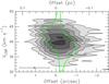 |
Fig. 17 Position-velocity diagram of the CH3CN 183−173 component towards the SMA1 core. The cut is made along a direction with PA = 37°, i.e. along the velocity gradient identified in Fig. 14. The contour levels range from 0.61 to 4.1 in steps of 0.6 Jy beam-1. The horizontal and vertical bars in the bottom left indicate the spatial and velocity resolutions, respectively. The solid green curves encompass the region of the plot inside which emission is expected if the gas undergoes Keplerian rotation about and free-fall infall onto a massive star with mass 83 M⊙. |
Although the simple scenario depicted here is far from being unique, the pattern is consistent with the line emission, once the limited angular resolution is taken into account. This shows that one cannot rule out the possibility that the infalling material is settling onto a centrifugally supported disk in the innermost regions of the HMC.
4.3. Nature of the SMA1 core
What is the stellar content of the HMC? Does it consist of one (or a few) massive stars, or does the core hosting a cluster of lower mass stars? Our findings do not allow us to draw any firm conclusion, as the molecular gas cannot be investigated with sufficient resolution and only a loose upper limit can be set on the HMC luminosity. With the advent of the next generation of large telescopes, it will be possible to overcome these problems, but at present we can only make speculations.
We have seen in Sect. 4.1 that no free-free emission is detected towards the HMC and that this may imply that no star earlier than B0.5 is present in the core or that the star is still in a pre-UC HII region phase. If the scenario proposed in Sect. 4.2 is correct, we are dealing with a well defined system, consisting of a massive core undergoing infall and rotating about a water maser jet/H13CO+ outflow. This symmetric structure and the high mass-accretion rate derived suggest that only a few high-mass YSOs might be located at the center of this system, rather than a cluster with a significant contribution from low-mass stars. This hypothesis is supported by comparing the fragmentation timescale, tfrag, with the free-fall time, tff, of the HMC. The former can be evaluated to be the ratio of the core diameter to the line width of a typical HMC tracer, e.g. CH3CN, i.e., tfrag = 0.14 pc/10 km s-1 ≃ 1.4 × 10⁴ yr. The latter is calculated for a mean H2 density of ~4 × 107 cm-3, and is tff ≃ 6 × 10³ yr. Because tfrag ~ 2tff, we argue that fragmentation may be partially inhibited during the collapse.
We point out that the previous discussion has a limited validity, as it is mostly based on qualitative arguments and neglects the effect of the magnetic field, which might contribute significantly to stabilize the core against gravitational collapse. Nonetheless, we believe that our findings lend support to the idea that the stellar content of the core could be biased towards very young, OB-type stars.
5. Conclusions and future perspectives
We have performed deep continuum imaging from the centimeter to the sub-millimeter regime of the G 19.61−0.23 high-mass star-forming region. Our observations have confirmed the existence of a large number of UC HII regions, as well as that of a HMC. The latter is resolved into three cores, with one of these (here called “the HMC”) being ~10 times more massive than the others. We have also mapped the region in a number of molecular lines at 3 mm and 890 μm, most of which appear to trace the three cores. Star formation is likely to occur not only in the HMC (SMA1), but also in the other two cores (SMA2, SMA3), as supported by the existence of a bipolar outflow seen in the SiO (2−1) line towards SMA2.
The CH3CN (18–17) line emission reveals a velocity gradient across SMA1, roughly perpendicular to a water maser jet and bipolar H13CO+ outflow directed in the SE−NW direction. We conclude that this velocity gradient is caused by rotation about the jet/outflow axis. We have also confirmed the existence of an inverse P-Cygni profile in the 13CO (3−2) line, previously detected by Wu et al. (2009), and recover a similar profile also in the C18O (3−2) line. This redshifted absorption strongly suggests that the SMA1 core is infalling – beside rotating – with a mass accretion rate >3 × 10⁻³ M⊙ yr-1. We conclude that very young OB-type stars are probably forming inside the HMC.
The study presented here is an excellent benchmark of what will be feasible, with much better resolution and sensitivity, with new generation instruments. Deep unbiased surveys of selected high-mass star forming regions will permit us to improve our knowledge of the OB star formation process, identifying newly formed stars by means of their free-free continuum emission and investigating at the same time the structure and velocity field of the molecular cores associated with them.
The National Radio Astronomy Observatory is a facility of the National Science Foundation operated under cooperative agreement by Associated Universities, Inc.
The Nobeyama Radio Observatory is a branch of the National Astronomical Observatory of Japan, operated by the Ministry of Education, Culture, Sports, Science and Technology, Japan.
Research at the Owens Valley Radio Observatory is supported by the National Science Foundation through NSF grant AST 02-28955.
The Submillimeter Array is a joint project between the Smithsonian Astrophysical Observatory and the Academia Sinica Institute of Astronomy and Astrophysics and is funded by the Smithsonian Institution and the Academia Sinica.
Acknowledgments
The authors are grateful to the referee, Dr. S. Curiel, and the editor, Dr. C. M. Walmsley, for their constructive comments to the manuscript. The authors sincerely acknowledge S. Takahashi, M. Momose, L. Testi, and C. Codella for their contribution at early stage of this study as co-authors of Paper I. In particular, S. Takahashi and M. Momose performed the NMA observations and calibrated most of the visibility data. The authors also acknowledge M. J. Claussen and G. V. Moorsel for their extensive help in VLA observations, especially handling the EVLA antenna data, D. Fong for his help in calibrating the SMA data, J. M. Carpenter and J. Lamb for their help in combining the OVRO and NMA visibilities, and A. I. Sargent and P. T. P. Ho for their fruitful comments and encouragement. R.S.F. is supported by a Grant-in-Aid from the Ministry of Education, Culture, Sports, Science and Technology of Japan (No. 20740113).
References
- Acord, J. M., Walmsley, C. M., & Churchwell, E. 1997, ApJ, 475, 693 [NASA ADS] [CrossRef] [Google Scholar]
- Beltrán, M. T., Cesaroni, R., Neri, R., et al. 2004, ApJ, 601, L187 [NASA ADS] [CrossRef] [Google Scholar]
- Beltrán, M. T., Cesaroni, R., Neri, R., et al. 2005, A&A, 435, 901 [NASA ADS] [CrossRef] [EDP Sciences] [Google Scholar]
- Beltrán, M. T., Cesaroni, R., Codella, C., et al. 2006, Nature, 443, 427 [NASA ADS] [CrossRef] [PubMed] [Google Scholar]
- Beuther, H., Schilke, P., Sridharan, T. K., et al. 2002, A&A, 383, 892 [NASA ADS] [CrossRef] [EDP Sciences] [Google Scholar]
- Beuther, H., Zhang, Q., Sridharan, T. K., & Chen, Y. 2005, ApJ, 628, 800 [NASA ADS] [CrossRef] [Google Scholar]
- Cabrit, S., & Bertout, C. 1992, A&A, 261, 274 [Google Scholar]
- Cesaroni, R., Walmsley, C. M., & Churchwell, E. 1992, A&A, 256, 618 [NASA ADS] [Google Scholar]
- Cesaroni, R., Galli, D., Lodato, G., Walmsley, C. M., & Zhang, Q. 2007, Protostars and Planets V, 197 [Google Scholar]
- Churchwell, E., Walmsley, C. M., & Cesaroni, R. 1990, A&AS, 83, 119 [Google Scholar]
- Codella, C., Testi, L., & Cesaroni, R. 1997, A&A, 325, 282 [NASA ADS] [Google Scholar]
- Dickman, R. L. 1978, ApJS, 37, 407 [NASA ADS] [CrossRef] [Google Scholar]
- Downes, D., Wilson, T. L., Bieging, J., & Wink, J. 1980, A&AS, 40, 379 [NASA ADS] [Google Scholar]
- Forster, J. R., & Caswell, J. L. 2000, ApJ, 530, 371 [NASA ADS] [CrossRef] [Google Scholar]
- Furuya, R. S., Kitamura, Y., Wootten, H. A., et al. 2000, ApJ, 542, L135 [NASA ADS] [CrossRef] [Google Scholar]
- Furuya, R. S., Kitamura, Y., Wootten, H. A., Claussen, M. J., & Kawabe, R. 2001, ApJ, 559, L143 [NASA ADS] [CrossRef] [Google Scholar]
- Furuya, R. S., Cesaroni, R., Takahashi, S., et al. 2005a, ApJ, 624, 827 [NASA ADS] [CrossRef] [Google Scholar]
- Furuya, R. S., Kitamura, Y., Wootten, A., Claussen, M. J., & Kawabe, R. 2005b, A&A, 438, 571 [NASA ADS] [CrossRef] [EDP Sciences] [Google Scholar]
- Furuya, R. S., Kitamura, Y., & Shinnaga, H. 2006, ApJ, 653, 1369 [NASA ADS] [CrossRef] [Google Scholar]
- Furuya, R. S., Cesaroni, R., Takahashi, S., et al. 2008, ApJ, 673, 363 [NASA ADS] [CrossRef] [Google Scholar]
- Garay, G., Reid, M. J., & Moran, J. M. 1985, ApJ, 289, 681 [NASA ADS] [CrossRef] [Google Scholar]
- Garay, G., Moran, J. M., Rodriguez, L. F., & Reid, M. J. 1998, ApJ, 492, 635 [NASA ADS] [CrossRef] [Google Scholar]
- Georgelin, Y. M., & Georgelin, Y. P. 1976, A&A, 49, 57 [NASA ADS] [Google Scholar]
- Girart, J. M., Beltrán, M. T., Zhang, Q., Rao, R., & Estalella, R. 2009, Science, 324, 1408 [NASA ADS] [CrossRef] [PubMed] [Google Scholar]
- Goldsmith, P. F., & Langer, W. D. 1999, ApJ, 517, 209 [NASA ADS] [CrossRef] [Google Scholar]
- Hofner, P., & Churchwell, E. 1996, A&AS, 120, 283 [NASA ADS] [CrossRef] [EDP Sciences] [Google Scholar]
- Keto, E. R., Ho, P. T. P., & Haschick, A. D. 1988, ApJ, 324, 920 [NASA ADS] [CrossRef] [Google Scholar]
- Kolpak, M. A., Jackson, J. M., Bania, T. M., Clemens, D. P., & Dickey, J. M. 2003, ApJ, 582, 756 [NASA ADS] [CrossRef] [Google Scholar]
- Kurtz, S., Cesaroni, R., Churchwell, E., Hofner, P., & Walmsley, C. M. 2000, Protostars and Planets IV, 299 [Google Scholar]
- López-Sepulcre, A., Codella, C., Cesaroni, R., Marcelino, N., & Walmsley, C. M. 2009, A&A, 499, 811 [NASA ADS] [CrossRef] [EDP Sciences] [Google Scholar]
- Molinari, S., Brand, J., Cesaroni, R., & Palla, F. 2000, A&A, 355, 617 [NASA ADS] [Google Scholar]
- Muench, A. A., Lada, E. A., Lada, C. J., & Alves, J. 2002, ApJ, 573, 366 [NASA ADS] [CrossRef] [Google Scholar]
- Panagia, N. 1973, AJ, 78, 929 [NASA ADS] [CrossRef] [Google Scholar]
- Pandian, J. D., Momjian, E., & Goldsmith, P. F. 2008, A&A, 486, 191 [NASA ADS] [CrossRef] [EDP Sciences] [Google Scholar]
- Pearson, J. C., & Mueller, H. S. P. 1996, ApJ, 471, 1067 [NASA ADS] [CrossRef] [Google Scholar]
- Qin, S.-L., Wu, Y., Huang, M., et al. 2010, ApJ, 711, 399 [NASA ADS] [CrossRef] [PubMed] [Google Scholar]
- Remijan, A., Shiao, Y.-S., Friedel, D. N., Meier, D. S., & Snyder, L. E. 2004, ApJ, 617, 384 [NASA ADS] [CrossRef] [Google Scholar]
- Torrelles, J. M., Gomez, J. F., Rodriguez, L. F., et al. 1996, ApJ, 457, L107 [NASA ADS] [CrossRef] [Google Scholar]
- Walmsley, M. 1995, Rev. Mex. Astron. Astrofis. Conf. Ser., 1, 137 [NASA ADS] [Google Scholar]
- Wilson, T. L., & Rood, R. T. 1994, ARA&A, 32, 191 [NASA ADS] [CrossRef] [Google Scholar]
- Wood, D. O. S., & Churchwell, E. 1989, ApJ, 340, 265 [NASA ADS] [CrossRef] [Google Scholar]
- Wu, Y., Qin, S.-L., Guan, X., et al. 2009, ApJ, 697, L116 [NASA ADS] [CrossRef] [Google Scholar]
- Zapata, L. A., Palau, A., Ho, P. T. P., et al. 2008, A&A, 479, L25 [NASA ADS] [CrossRef] [EDP Sciences] [Google Scholar]
Appendix A: Rotation diagram analysis of the SiO lines
We estimated the excitation temperature of the SiO molecule from the (2−1), (3−2), and (5−4) transitions (Fig. A.1; J. M. Acord, personal communication) that had been observed simultaneously with the IRAM 30 m telescope. In this way, problems due to relative gain calibration and pointing errors were minimized. Following Acord et al. (1997), we applied the “rotation diagram” method, whose advantages and limitations are discussed in detailed in Goldsmith & Langer (1999). For this purpose, in Fig. A.2 we plot the logarithm of the column density in the lower level of each transition, divided by the corresponding statistical weight, against the energy of the upper level, Eu. The column densities were derived from the line intensities based on the assumption of optically thin emission. The column densities were also corrected for the different beam-filling factors of the three lines, assuming the source to be point-like and referring all measurements to the 28″ beam at the frequency of the (2−1) line.
The slope of the linear fit to the data, 1/T, infers the “rotational temperature” (Trot) of the SiO molecules, which is likely to be an underestimate of the kinetic temperature of the H2 gas (see e.g. Acord et al. 1997). The data are well fitted by a straight line, which indicates that the method used is likely correct, although the SiO molecule is known to be subthermally excited as noted above. We obtain Trot ≃ 20 K and a total SiO beam averaged column density of 4.6 × 1013 cm-2.
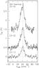 |
Fig. A.1 Spectra of thermal (v = 0) emission of the SiO molecule towards G 19.61−0.23 taken with the IRAM 30 m telescope (J. M. Acord personal communication) on a main-beam brightness temperature (Tmb) scale. The vertical dashed-line indicates the systemic velocity (Vsys) of VLSR = 41.6 km s-1. |
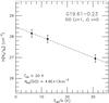 |
Fig. A.2 Rotation diagram of the SiO thermal emission shown in Fig. A.1. The dashed line is the best-fit to the data. The values of the rotation temperature and column density thus obtained are given in the bottom left of the figure. |
All Tables
All Figures
|
Fig. 1 Continuum emission maps toward the G 19.61−0.23 high-mass star-forming region. All the contour levels are drawn with ± 7σ·2n, where σ is the rms noise level of the image (Table 1) and n = 0,1,2,... . The wavelength and FWHM of the synthesized beam are indicated in the bottom right corner of each panel. See Table 1 for the values of the synthesized beams. |
| In the text | |
|
Fig. 2 Continuum emission maps at 890 μm taken with SMA toward G 19.61−0.23 with a) natural weighting and b) uniform weighting. The solid contours start at the 3σ level and increase in steps of + 2σ up to the 50% level for a clarity of the maps. The dashed contours start at the −3σ level and decrease in steps of −2σ. The image noise levels are 54.1 and 34.9 mJy beam-1 for panels a) and b), respectively. The sensitivity of the uniformly weighted map is better than that of the naturally weighted map, probably because the visibilities have not been weighted taking into account the system temperature of each antenna (see Sect. 2.5). The synthesized beams are shown in the bottom right corners (1''̣38 × 1''̣22 with PA = −44° for natural weighting; 0''̣85 × 0''̣78 with PA = −32° for uniform weighting). |
| In the text | |
|
Fig. 3 Comparison of the 6 cm (greyscale plus white contour), 3.8 cm (magenta contour), and 1.3 cm (yellow contour) continuum emission maps generated with the common minimum UV distance of 13.3 kλ (see Sect. 3.1.3). Contour intervals for the cm maps and the submm map are the same as those in Figs. 1 and 2, respectively, where the 1σ noise levels are 0.23, 0.18, and 0.36 mJy beam-1 and the beams 0''̣433 × 0''̣321, 0''̣262 × 0''̣195, and 0''̣344 × 0''̣251, for the 6.0, 3.8, and 1.3 cm maps, respectively. The largest of the three beams is shown in the bottom right. The filled red rectangules and the double red circles indicate the peak positions of the 3 mm (Paper I) and 890 μm (Sect. 3.1.2) continuum emission, respectively. The filled green circles and light-blue triangles show the positions of the OH (Garay et al. 1985) and H2O (Hofner & Churchwell 1996) masers, respectively. Labels A and C refer to the UC HII regions (notation as in Paper I and references therein). The filled yellow circle associated with the UC HII region C indicates the peak position of the isolated 7 mm emission seen in Fig. 1e close to the HMC. |
| In the text | |
|
Fig. 4 First moment map of the H2O masers (color image) and maps of the continuum emission (color contours). The black contours overlayed on the maser velocity map correspond to the integrated intensity of the maser spots, with levels starting from the 5σ level with 5σ steps. The black, cyan, and magenta contours represent the first 3 contours of the 890 μm, 6 cm, and 3.8 cm continuum emission, respectively (the same as in Fig. 2). The yellow triangles and green-filled circles show, respectively, the positions of the H2O (Hofner & Churchwell 1996) and OH (Garay et al. 1985) masers. The numbers associated with the yellow triangles are used to identify the maser features as done by Hofner & Churchwell (1996). |
| In the text | |
|
Fig. 5 H2O maser spectra toward the maser features Nos. 1 and 2 obtained by integrating the emission inside the 5σ contour of each emission (see Fig. 4). The vertical dashed line indicates the systemic velocity (Vsys) of the cloud, VLSR = 41.6 km s-1. |
| In the text | |
|
Fig. 6 Total integrated intensity maps of the 13CO (3−2) (left panels) and C18O (3−2) (right panels) lines produced with natural (upper panels) and uniform (lower panels) visibility weighting functions. Note that the upper panels show the whole area of the G 19.61−0.23 star-forming region, while the lower panels magnify the region centered on the HMC (greyscale plus thin contour; see Table 2). For comparison purposes, the 7σ level contour of the 6 cm continuum (i.e., free-free) emission as in Fig. 1a is shown by thin green contours. The magenta stars indicate the peak positions of the three 890 μm continuum sources (Table 3). The contours of the CO isotopomer maps start from the 5σ level in steps of 3σ, where the 1σ noise levels are 1.9 and 1.8 Jy beam-1 km s-1 for the natural and uniform weighted 13CO maps, and 0.8 Jy and 1.7 beam-1 km s-1 for the natural and uniform weighted C18O maps, respectively. We integrated the emission over the LSR-velocity ranges 30.2 ≤ VLSR/km s-1 ≤ 42.2 for 13CO, and 34.7 ≤ VLSR/km s-1 ≤ 44.5 for C18O. All the other symbols are the same as those in Fig. 1. The emission seen in the top of the upper-panels is an artifact caused in the cleaning process. |
| In the text | |
|
Fig. 7 Spectra of four molecular lines in Tsb scale towards the peak of the 890 μm continuum emission, i.e., SMA1. The SiO and H13CO+ intensities are scaled by a factor 2.0. The vertical dashed line indicates the systemic velocity (Vsys) of the cloud, VLSR = 41.6 km s-1. In the CO isotopomers spectra, we mark the positions of all possible (molecular) lines, calculated assuming that they are emitted with velocity equal to Vsys (see Sect. 3.3.2). The thick horizontal blue and red bars denote the velocity intervals over which the line emission has been integrated to produce the maps in Figs. 9, 10, and 16. The emission seen around VLSR ≃ 70 km s-1 of the C18O spectrum probably originates in the HNCO line rather than CH |
| In the text | |
|
Fig. 8 Comparison of the absorption features seen in the 13CO (3−2) and HCO+ (1−0) lines toward the peak of the 890 μm continuum emission. For the sake of comparison, the interferometric 13CO (3−2) spectrum has been obtained after reconstructing the data with a synthesized beam equal to the single-dish beam of the HCO+ line observations with IRAM 30-m telescope (see Sect. 3.3.3). |
| In the text | |
|
Fig. 9 a) Integrated intensity map of the H13CO+ (1−0) bulk emission. The velocity range used for the integration is 35.5 ≤ VLSR/km s-1 ≤ 48.9. The interval between the thin-black contours is 2σ with the lowest contour corresponding to the 3σ level, where the 1σ rms noise is 0.53 Jy beam-1 km s-1. The thin-white contours are the 95% and 90% levels of the corresponding peak intensities, where the 90% levels correspond to the 7.5σ level. All the other symbols are the same as those in Fig. 6, and the numbers associated with the three maser spots to the west are the same as those used by Hofner & Churchwell (1996). The dashed box indicates the area shown in the right-hand panel. b) Overlay of the blue- and redshifted wing emission maps of the H13CO+ (1−0) emission. The contours are 2σ steps starting from the 3σ level. The blue- and redshifted wing emission maps were obtained by averaging the wing emission over the intervals 35.3 < VLSR/km s-1 < 37.9 and 43.1 < VLSR/km s-1 < 49.2, and their rms noise levels are 43.8 and 30.2 mJy beam-1, respectively. |
| In the text | |
|
Fig. 10 a) Integrated intensity map of the bulk emission of the SiO (2−1) v = 0 line (greyscale plus thin contours) observed with the OVRO and NMA interferometers. The green contours have the same meaning as in Fig. 6. The bulk emission has been integrated over the LSR-velocity range of 31.9 ≤ VLSR/km s-1 ≤ 48.4, and the rms noise level is 0.28 Jy beam-1 km s-1. The yellow stars represent the positions of SMA1, SMA2, and SMA3 (see Table 3). b) Overlay of the blue- and redshifted wing emission maps of the SiO (2−1) v = 0 emission. The contours are spaced by 2σ and start at the 3σ level. The blue- and redshifted wing emission maps have been obtained by averaging the wing emission over the intervals 21.1 < VLSR/km s-1 < 31.9 and 48.4 < VLSR/km s-1 < 58.0, and their rms noise levels are 11.6 and 13.9 mJy beam-1, respectively. The hatched ellipses in the bottom right indicates the FWHM of the synthesized beam (Table 2). |
| In the text | |
|
Fig. 11 Interferometric spectrum of the CH3CN and CH313CN (18−17) lines towards the peak position of the 890 μm continuum source, SMA1. The vertical bars above and below the spectrum indicate the rest-frequencies of the K components of the CH3CN and CH313CN J = 18−17 transitions. We also indicate other lines that may be blended with the methyl cyanide lines. |
| In the text | |
|
Fig. 12 Integrated intensity maps of the JK = 18K − 17K emission of the CH3CN (green contour) and CH313CN (magenta contour) lines. The black dashed contour corresponds to the absorptions region seen in the 13CO (3−2) line. The thin black contour represents the 7σ level of the uniform weighting 890 μm continuum emission map (Fig. 2b). All the transitions, except the CH3CN K = 0, 1, and 2 components, are not blended with other lines (see Fig. 11 for the spectrum). The contour intervals are spaced by 2σ and start from the 3σ level. In the CH3CN maps, we do not plot contours above the 17σ level to prevent saturation of the maps. The 1σ rms noise levels are 6.3, 1.4, 1.3, 0.33, and 0.17 mJy beam-1 km s-1 for the CH3CN (18−17) K = 0 to 2 emission, K = 3, K = 4, and CH313CN (18−17) K = 2, and K = 6, respectively. |
| In the text | |
|
Fig. 13 Rotation diagram obtained from the K = 0, 1, 2, 4, 5, and 6 components of the CH |
| In the text | |
|
Fig. 14 Maps of the line peak velocity (color) obtained from simultaneous Gaussian fits to the CH3CN and/or CH |
| In the text | |
|
Fig. 15 Plot of the brightness temperature in the synthesized beam of a Strömgren HII region, as a function of radius and Lyman continuum photon rate (see Sect. 4.1 for details). The curves correspond to the 3σ upper limits on the free-free continuum emission measured towards SMA1 at 4.86 GHz (blue), 8.42 GHz (green), and 22.273 GHz (red). Here the rms noise levels and the geometrical mean of the beam FWHPs adopted to plot are 230 μJy beam-1 at 5 GHz, 180 μJy beam-1 at 8 GHz, and 360 μJy beam-1 at 22 GHz. The labels to the right indicate the spectral types of the ZAMS stars with the corresponding value of NLy, according to Panagia (1973). |
| In the text | |
|
Fig. 16 The color maps are the same as in Fig. 14, while the superimposed solid blue and dashed red contours represent, respectively, the blueshifted emission and redshifted absorption seen in the 13CO (left panel) and C18O (right panel). To obtain these plots, we integrated the line over 3 velocity channels centered on the deepest absorption and the most intense emission, namely over the ranges: 34.2 ≤ VLSR/km s-1 ≤ 35.8 for the blueshifted 13CO emission, 43.8 ≤ VLSR/km s-1 ≤ 45.0 for the redshifted 13CO absorption, and 36.0 ≤ VLSR/km s-1 ≤ 38.4 for the blueshifted C18O emission, 44.0 ≤ VLSR/km s-1 ≤ 46.4 for the redshifted C18O absorption. These velocity ranges are outlined by the horizontal blue and red bars in Fig. 7. All the contours are in steps of ± 2σ and start from the ± 3σ level. The stars mark the peak positions of SMA1 and SMA2. See Sect. 4.2 for details. |
| In the text | |
|
Fig. 17 Position-velocity diagram of the CH3CN 183−173 component towards the SMA1 core. The cut is made along a direction with PA = 37°, i.e. along the velocity gradient identified in Fig. 14. The contour levels range from 0.61 to 4.1 in steps of 0.6 Jy beam-1. The horizontal and vertical bars in the bottom left indicate the spatial and velocity resolutions, respectively. The solid green curves encompass the region of the plot inside which emission is expected if the gas undergoes Keplerian rotation about and free-fall infall onto a massive star with mass 83 M⊙. |
| In the text | |
|
Fig. A.1 Spectra of thermal (v = 0) emission of the SiO molecule towards G 19.61−0.23 taken with the IRAM 30 m telescope (J. M. Acord personal communication) on a main-beam brightness temperature (Tmb) scale. The vertical dashed-line indicates the systemic velocity (Vsys) of VLSR = 41.6 km s-1. |
| In the text | |
|
Fig. A.2 Rotation diagram of the SiO thermal emission shown in Fig. A.1. The dashed line is the best-fit to the data. The values of the rotation temperature and column density thus obtained are given in the bottom left of the figure. |
| In the text | |
Current usage metrics show cumulative count of Article Views (full-text article views including HTML views, PDF and ePub downloads, according to the available data) and Abstracts Views on Vision4Press platform.
Data correspond to usage on the plateform after 2015. The current usage metrics is available 48-96 hours after online publication and is updated daily on week days.
Initial download of the metrics may take a while.