| Issue |
A&A
Volume 697, May 2025
|
|
|---|---|---|
| Article Number | A223 | |
| Number of page(s) | 20 | |
| Section | Extragalactic astronomy | |
| DOI | https://doi.org/10.1051/0004-6361/202452609 | |
| Published online | 22 May 2025 | |
The near-infrared spectral energy distribution of blue quasars: Determining what drives the evolution of the dusty torus
1
Dipartimento di Fisica e Astronomia, Università di Firenze, via G. Sansone 1, 50019 Sesto Fiorentino, Firenze, Italy
2
INAF – Osservatorio Astrofisico di Arcetri, Largo Enrico Fermi 5, I-50125 Firenze, Italy
3
INAF – Osservatorio di Astrofisica e Scienza dello Spazio di Bologna, via Gobetti 93/3, I-40129 Bologna, Italy
4
Dipartimento di Fisica e Astronomia, Università di Bologna, Via Gobetti 93/2, I-40129 Bologna, Italy
5
Dipartimento di Matematica e Fisica, Univeristà di Roma 3, Via della Vasca Navale, 84, 00146 Roma, Italy
⋆ Corresponding author: bartolomeo.trefoloni@unifi.it
Received:
14
October
2024
Accepted:
5
February
2025
A fundamental ingredient in the unified model of active galactic nuclei (AGN) is the obscuring torus, whose innermost, hottest region dominates the near infrared (NIR) emission. Characterising the change in the torus properties and its interplay with the primary AGN emission is key for our understanding of AGN physics, evolution, and classification. Its covering factor (CF) is largely responsible for the classification of AGN on the basis of the detection of broad emission lines. It is still not clear whether the torus properties evolve over time and how they relate with the accretion parameters of the nucleus. In this work, we aim at investigating the evolution of the NIR properties with the redshift (z) and the bolometric luminosity (Lbol) in a sample of AGN. To this end, we assembled a large dataset of ∼36 000 type 1 AGN between 0.5 < z < 2.9 and 45.0 < log(Lbol/(erg s)) < 48.0 with UV, optical, and near-infrared photometry. We produced average spectral energy distributions (SED) in different bins of the z − Lbol parameter space to estimate how the NIR SED evolves according to these parameters. We find that the NIR luminosity decreases for increasing Lbol at any redshift. At the same time, the shape of the NIR SED in our sample is consistent with a non-evolution with z. As a consequence, all the explored proxies for the CF exhibit significant anti-correlations with Lbol, but not with z. Additionally, the CF also shows a shallower anti-correlation with the Eddington ratio (λEdd), yet the current systematic uncertainties, as well as the limited dynamical range, do not allow us to precisely constrain the role of the Eddington ratio. Lastly, we derived the covering factor from the ratio between the NIR and optical luminosity and we employed it to set a lower limit for the X-ray obscuration at different redshifts.
Key words: galaxies: active / galaxies: nuclei / quasars: general / quasars: supermassive black holes
© The Authors 2025
 Open Access article, published by EDP Sciences, under the terms of the Creative Commons Attribution License (https://creativecommons.org/licenses/by/4.0), which permits unrestricted use, distribution, and reproduction in any medium, provided the original work is properly cited.
This article is published in open access under the Subscribe to Open model. Subscribe to A&A to support open access publication.
1. Introduction
Supermassive black holes (SMBH) efficiently accreting gas and dust are known as active galactic nuclei (AGN). The spectral energy distribution (SED) of these sources covers the whole electromagnetic spectrum, with two noticeable peaks: the ‘big blue bump’ (BBB, Shields 1978) in the optical–UV, and an infrared bump around 10 μm (e.g. Edelson & Malkan 1986; Barvainis 1987). The former is thought to be produced by the accretion disc powering the AGN, while the latter arises because of some colder gaseous and dusty material re-emitting the primary AGN continuum in the infrared.
In the current standard picture, the unified model (Antonucci 1993; Urry & Padovani 1995), the observational diversity of AGN in terms of spectral properties, is explained as the result of different lines of sight to the central engine. A key ingredient of the unified model is the obscuring torus, a dusty and gaseous structure on parsec scales, surrounding the accretion disc. In this framework, an unobscured (type 1) AGN is observed when the line of sight does not cross the obscuring material; in the case of an obscured (type 2) AGN the inner engine is hidden by the toroidal obscurer.
This observational classification can also be interpreted in terms of escape probability of the light through the spatial distribution of clumpy elements forming the torus, thus allowing for a less strict division between type 1 and type 2 AGN (see e.g. Ramos Almeida et al. 2011; Mateos et al. 2016). An outer tilted torus on scales of ∼100 pc (McLeod & Rieke 1995; Maiolino & Rieke 1995) can also be included to account for intermediate AGN types.
A critical parameter defining the properties of the torus is the covering factor (CF), which is generally defined as the fraction of the whole solid angle covered by an obscuring structure (Ω/4π, e.g. Hamann et al. 1993). Although the definition of the covering factor is purely geometrical, on a practical level there are different routes to estimate this parameter, taking advantage of several techniques across different wave bands.
In the X-ray surveys, the fraction of obscured sources (generally those with log(NH/cm−2) > 22) is used as a proxy for the mean covering factor at a given luminosity, provided that the sample has a high enough completeness level, and under the hypothesis of randomly oriented AGN in the sky (e.g. Ueda et al. 2003, 2014; La Franca et al. 2005; Hasinger 2008; Burlon et al. 2011; Malizia et al. 2012; Merloni et al. 2014). A similar argument has been used to estimate the CF as the ratio of narrow-line (type 2) to broad-line (type 1) AGN, based on the optical spectrum (Simpson 2005; Toba et al. 2014).
In addition, by considering that the intrinsic UV luminosity of the AGN is reprocessed by the gaseous and dusty torus and re-emitted in the infrared (e.g. Maiolino et al. 2007; Treister et al. 2008; Gandhi et al. 2009), the covering factor can thus be derived as the ratio of the reprocessed infrared luminosity to the intrinsic AGN emission. However, this ratio does not take into account the complicated anatomy of the covering material (Granato & Danese 1994). Early analytical models employed a simplistic continuous toroidal screen (Pier & Krolik 1992), but the need for a more irregular gas and dust distribution was already clear. The strong nuclear radiation field is expected to break a continuous torus into smaller clumps (Krolik & Begelman 1988) whose turbulent motion helps in stabilising a geometrically thick structure (Beckert & Duschl 2004). Deriving the CF is far less straightforward for a non-homogeneous (i.e. clumpy) distribution of the clouds composing the torus (Nenkova et al. 2008a,b; Lusso et al. 2013; Netzer 2015), and detailed radiative transfer modelling (Stalevski et al. 2016) showed that the bare infrared-to-optical luminosity ratio systematically underestimates low CFs and overestimates high CFs in the case of type 1 AGN.
Critical pieces of information about the torus properties have also been gathered by successfully applying torus models to reproduce observations of low-redshift Seyferts and luminous AGN both in the infrared (e.g. Mor et al. 2009; Hönig et al. 2010; Alonso-Herrero et al. 2011, 2021; Ramos Almeida et al. 2011; Feltre et al. 2012; Zhuang et al. 2018; Ichikawa et al. 2019; González-Martín et al. 2019; García-Bernete et al. 2019, 2022) and in X-rays (see e.g. Ricci & Paltani 2023, but also Ramos Almeida & Ricci 2017 for a more comprehensive review). In the latter case, both the iron Kα emission line and the ∼30 keV Compton hump have been used to constrain the geometry of the circumnuclear material (Ricci et al. 2014; Gandhi et al. 2015).
In a dynamical picture, the properties of the torus are expected to vary according to the accretion parameters of the AGN (i.e. the bolometric luminosity Lbol, the black hole mass MBH, and the Eddington ratio λEdd). A simple evolutionary scenario predicts that its covering factor should decrease with increasing luminosity, which is the idea of the receding torus (Lawrence 1991), or a luminosity-dependent unified model (Ueda et al. 2003). In this picture, the radiation field produced in the innermost regions of the AGN is capable of directly shaping the morphology of the gaseous and dusty surrounding material. At the same time, efficient accretion and high luminosity are expected to be conducive conditions for the launch of powerful accretion-disc winds, directly driven by the nuclear activity (e.g. Proga 2005; Zubovas & King 2013; Nardini et al. 2015, 2019; King & Pounds 2015; Tombesi et al. 2015), which could be equally able to shape the circumnuclear environment in episodic events rather than on galactic timescales. A dependence on the accretion rate is also supported by recent studies (see e.g. Ricci et al. 2023 and references therein) arguing that the actual driver of the covering factor decrease might be the Eddington ratio rather than the bare bolometric luminosity, with the former being equivalent to an effective (mass-normalized) luminosity.
Although the properties of the torus, dominating the infrared SED of AGN, are expected to vary with the luminosity and/or the Eddington ratio, credible possible evolution with redshift has not yet been found. From a cosmological standpoint, there is growing evidence that the UV and optical SED properties in quasars do not appreciably evolve with redshift. Luminous blue AGN shining at high redshift are indeed remarkably similar to those observed locally, in terms of continuum properties (e.g. Kuhn et al. 2001; Mortlock et al. 2011; Hao et al. 2013; Shen et al. 2019; Yang et al. 2021; Trefoloni et al. 2024b) and of line properties (e.g. Croom et al. 2002; Fan et al. 2004; Nagao et al. 2006; Stepney et al. 2023). These findings are echoed in the infrared, where several works showed that the average SEDs made of samples over wide redshift intervals, up to z ∼ 4, exhibit quite similar shapes also in the NIR and mid-infrared (MIR) ranges (e.g. Elvis et al. 1994; Richards et al. 2006; Krawczyk et al. 2013, but see also Bianchini et al. 2019 for recent updates from a larger MIR sample). This evidence is also confirmed by other sparse samples at z ≳ 5, which exhibit NIR properties closely resembling those of the bulk of the quasar population at lower redshifts (Leipski et al. 2014), although with the noticeable exception of hot dust deficient quasars (e.g. Jiang et al. 2010; Hao et al. 2011). However, a systematic investigation of the NIR properties and their interplay with the main optical and UV continuum, while separately analysing the effects of luminosity and redshift over wide intervals has not yet been undertaken for a large sample of blue unobscured AGN.
For this work our aim was to investigate separately the possible evolution of the NIR SED in a sample of blue type 1 AGN with the accretion parameters (Lbol, λEdd) and the redshift, taking advantage of a large complete dataset purposefully assembled. In particular, we employed this large sample to address the following: i) investigating the evolution with Lbol and z of the NIR SED in blue quasars; ii) understanding how the covering factor in quasars evolves separately with z and with Lbol; iii) exploring the tentative anti-correlation between CF and λEdd.
The paper is structured as follows. A brief summary about the selection of the quasar sample is provided in Sect. 2, whilst the analysis performed on the sample SED is described in Sect. 3. The results are discussed in Sect. 4, and our conclusions are drawn in Sect. 5.
Throughout this paper we adopt a flat ΛCDM cosmology with H0 = 70 km s−1 Mpc−1, ΩΛ = 0.7, and Ωm = 0.3. Correlations are considered significant when yielding p-values lower than 0.01, corresponding to ∼2.6σ in the case of Normal approximation, under the null-hypothesis of non-correlation.
2. The dataset
With the aim of building a dataset covering the rest-frame emission from the UV to the IR for a large sample, we gathered and cross-matched photometric data from different surveys. Here we briefly highlight the building blocks of the final sample.
The starting sample is the Sloan Digital Sky Survey (SDSS) DR7 (Shen et al. 2011), which samples the rest-frame optical and UV wavelengths, where the AGN SED is dominated by the disc emission. This contains ∼106 000 quasars with both photometric and spectral data in the five SDSS bands (Fukugita et al. 1996) brighter than Mi < −22.0. Although newer releases have been produced, we opted for the SDSS DR7 catalogue as it offers a subsample of roughly 50 000 objects which abide by a uniform selection criterion, defined using the final quasar target selection algorithm described in Richards et al. (2002a), identified by the flag UNIFORM = 1 in the catalogue. This avoids the uneven sampling along the redshift axis and the selection criteria optimised to map the large-scale structure traced by the Lyα forest, which instead characterise the later BOSS (Dawson et al. 2012) and eBOSS (Dawson et al. 2016) surveys. At the same time, the SDSS selection algorithm claims a completeness close to ∼90% below mi < 19.1 at z < 2.9 (see Sect. 4.1 in Richards et al. 2002b for the related caveats), and this protects this work from incompleteness biases. With the aim of further increasing the quality of the sample we eventually opted for a magnitude cut at mi ≤ 19.0. Data in the u and z filters were corrected for the reported shifts in their zeropoints1.
The near- and mid-infrared bands (∼1–25 μm) are crucial when investigating the emission of the innermost hot region of the torus, which dominates the SED of luminous AGN in this band. At these wavelengths the AllWISE catalogue (Cutri et al. 2021) is the largest dataset available. This catalogue was produced from the collection of the Wide Infrared Survey Explorer (WISE, Wright et al. 2010) observations. We cross-matched this sample with the SDSS one adopting an optimal 2″ matching radius (see Sect. 2.2 in Krawczyk et al. 2013), which gives ∼97% of matches. For a typical quasar SED, the WISE filters have effective wavelengths 3.36 μm (W1), 4.61 μm (W2), 11.82 μm (W3) and 22.13 μm (W4). To improve the quality of the NIR data, we also required at least S/N = 2 in the W3 band, a requirement easily met in both W1 and W2. More details about the reliability of the WISE photometry and our NIR quality cuts can be found in Appendix A. Although the features of the AGN SED we are interested in are already well covered by these two surveys, we complemented the sample with other near-infrared and UV data. In particular, we added the UV points from the Galaxy Evolution Explorer (GALEX, Martin et al. 2005). The observed-frame reference wavelengths of the GALEX filters are 1528 Å (FUV) and 2271 Å (NUV), yielding respectively 38 000 and 45 000 detections which helped to probe the peak of the disc emission especially in the low-redshift regime. In the near-infrared band the main contributions to the AGN SED come from the low-energy tail of the disc and the hot dust from the torus, with some contamination from the host galaxy stellar emission being observed in low-luminosity AGN, below the quasar regime. We covered this region using NIR photometry from both the UKIRT (United Kingdom Infrared Telescope) Infrared Deep Sky Survey (UKIDSS; Lawrence et al. 2007) and the Two Micron All Sky Survey (2MASS; Skrutskie et al. 2006). These two supplementary datasets provided photometric data for roughly 11 300 and 10 000 sources in the YJHK and JHK bandpasses, respectively.
All available photometry was also corrected for Galactic extinction adopting the Fitzpatrick (1999) extinction curve and the extinction values from Schlafly & Finkbeiner (2011). The fraction of sources in each wave band that survives the selection cuts, described in the next Section, is reported in the legend of Fig. 1.
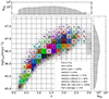 |
Fig. 1. log(Lbol)–z plane for the sources surviving the binning selection and the colour cut (see text for details). The final sample spans roughly 2.5 decades in bolometric luminosity and covers up to z ∼ 2.9. The data are randomly coloured if the bin contains more than 30 objects to make the binning clearer. The black diamonds mark the average z and log(Lbol) values. The legend reports the fraction of sources having data in the labelled band. Since the sample is based on the cross-match between the SDSS and the AllWISE catalogues, all objects have data in the bands covered by these surveys, while only a minority have a full coverage across the several wave bands. |
3. Methods
Here we describe the methods employed to correct the sample photometry for systematic effects and explain the subsequent analyses.
3.1. The parameter space
The key point of this study is the effort to disentangle the effects of the luminosity and the redshift in shaping the NIR emission from dusty torus of quasars. To achieve this goal, the sample was analysed in the log(Lbol)–z plane2, as shown in Fig. 1, using the reference values for each object tabulated in the latest SDSS spectral catalogue (Wu & Shen 2022). We note that when referring to log(Lbol) we mean the luminosity evaluated via some bolometric correction in the form kbol λLλ. In the following, we introduce further quantities designating the integrated accretion disc luminosity. Overall, the sample spans a wide region in terms of both redshift (0.1 < z < 2.9) and bolometric luminosity (45 < log(Lbol) < 47.6) as highlighted by Fig. 1. In order to study the evolution of the torus emission in the parameter space, we divided the distribution in bins of width Δz = 0.2 and Δlog(Lbol) = 0.2. The width of the bins is much larger than the typical uncertainty on the redshift, which is of the order of 0.1%, while it is similar to the typical uncertainty on Lbol, computed adopting monochromatic bolometric corrections (Richards et al. 2006).
3.2. Colour selection
The importance of the colour cut when aiming at isolating the intrinsic (i.e. not biased by extinction) quasar emission has been discussed in several works (see for instance Lusso et al. 2020, and references therein). We chose to apply a colour cut to address two main issues: 1) strong contamination from the host galaxy, which is also addressed in Sect. 3.3.2, and 2) dust reddening. Both these effects concur to make the observed SED of a quasar flatter than the intrinsic, polluting the broadband information about the relative importance of the torus emission. To tackle these issues we adopted an analogous procedure to that described in Sect. 5.1 of Lusso et al. (2020). In brief, for each object we computed the slope Γ1 of a log(ν)–log(νLν) power law in the rest frame 0.3–1 μm range, and the analogous slope Γ2 in the 1450–3000 Å range. We selected all the objects in the Γ1–Γ2 plane residing in the circle with center in the reference values for a typical quasar (Γ1 = 0.82, Γ2 = 0.40; Richards et al. 2006) and a reddening corresponding to E(B − V)≲0.1 assuming an SMC extinction curve (Prevot et al. 1984). The colour selection retained 90% of the sources, and it is shown in Fig. 2. In this figure, we also highlight the effect of increasing reddening on the observed colours of a SED with typical values of Γ1 and Γ2. This selection, aimed at avoiding the effects of extinction, does not affect any of our conclusions, as shown in Sect. 4.2. The sources surviving this final cut represent the starting sample for our analyses, and amount to 36 000 objects.
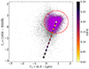 |
Fig. 2. Γ1–Γ2 plane for the sources satisfying the colour cut (magenta dots within the red circle). The light yellow square marks the average values reported in Richards et al. (2006) for blue unobscured quasars, while increasingly darker colours denote higher levels of reddening as labelled in the colour bar. |
3.3. Photometric corrections
Photometric data convolve the spectral information through band-pass filters. This causes the individual features, easily recognizable in a moderate-quality spectrum, to be instead mixed up in photometric points. Since we are mostly concerned in building the SED of the bare AGN disc and torus emission for each source of the sample, we needed to apply corrections for several effects. In detail, we took into account 1) the contribution from emission lines, 2) the host galaxy emission, 3) the inter-galactic medium (IGM) extinction. We accounted for each of these effects independently.
Generally speaking, the corrections α applied to each photometric point have the following expression:
Here Lf = ∫fλLλ|λ = λobs Sλobs dλobs is the total luminosity (i.e. λLλ) integrated through the observed-frame normalised pass-band of the filter f. The filter transmission curve Sλobs was simulated using the PYPHOT3 Python package4.
3.3.1. Line emission
The line emission is produced in the gas clumps rapidly moving around the SMBH on parsec scales in the BLR in the case of broad permitted lines. Both permitted and forbidden lines are also produced on galactic scales in the narrow-line region (NLR). These features act as contaminants in the photometric data when trying to isolate the AGN continuum emission. In order to subtract the emission line contribution in each filter, we considered the emission of a typical blue quasar, based on the Vanden Berk (2001) template Tλ. We built a model containing the bare power-law continuum ( ) and another one containing the power-law continuum plus the emission lines, the UV and optical iron pseudo-continua, and the Balmer continuum (
 ). We only corrected for the effect of the emission lines between 1200–7000 Å, where the strongest line contribution is expected, while we did not correct for the 9.7 μm feature (expected to be in emission in the case of type 1 AGN) in the IR as this falls outside of the wavelength range of interest for estimating the CF (see Sect. 3.5). For each photometric filter f the emission lines correction αEL was evaluated as:
The resulting luminosity in each filter is lower than or equal to the uncorrected one after applying this correction. An example of the result of this correction for a z = 1.0 quasar is shown in Fig. 3. Here we did not perform a luminosity-dependent emission line correction to take into account the anti-correlation between the emission line equivalent width and the luminosity (i.e. the Baldwin effect, Baldwin 1977). However, we note that, with respect to our results, this is a conservative approach. If we qualitatively assume weaker emission lines at higher Lbol (and z), smaller corrections would be implied and, consequently, intrinsically brighter disc luminosities. This, in turn, would translate into even lower torus-to-disc ratios at high Lbol, thus strengthening our conclusions (see Sect. 4.2).
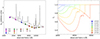 |
Fig. 3. Left: Pass-band integrated luminosity of the template with (empty diamonds) and without (filled diamonds) emission lines for a z = 1.0 quasar, according to the Vanden Berk (2001) template. Right: IGM transmission curves at different redshifts colour-coded as described in the legend. |
3.3.2. Host galaxy emission
The observed flux in each filter comes from the combination of the host galaxy and the AGN emission. However, luminous AGN (Lbol ≳ 1046 erg s−1) are expected to completely outshine their host galaxy. Since our sample is mostly composed of luminous quasars we decided not to apply any correction for the host galaxy contamination. Here we justify this assumption.
Several authors attempted a spectral decomposition to disentangle the AGN and the host galaxy contributions (e.g. Berk et al. 2006; Calderone et al. 2017; Rakshit et al. 2020; Jalan et al. 2023). The results vary slightly depending on the sample, the technique, and crucially on the S/N of the spectra employed for the de-composition (see e.g. Sect. 3.3 in Jalan et al. 2023). However, there is general agreement for quasars above Lbol = 1046 erg s−1 to completely outshine the galactic component. Different works employing a spectra decomposition found the host galaxy fraction, defined as  to be of the order of ≲15% at 5100 Å. These results are in line with independent estimates, such as those reported in Vanden Berk (2001) based on the strength of the Ca IIλ3933 and Na Iλ5896, which suggest a galactic contribution of the order of 7–15% for their sample, whose selection is similar to ours. Notably, this fraction progressively decreases at shorter wavelengths where the peak of the disc emission, which dominates the integrated disc luminosity, is observed. Additionally, also the colour cut plays a role in selecting sources where the galaxy contamination is minor (Lusso et al. 2020). As a more quantitative estimate of the possible residual (i.e. still present after the colour cut) galactic contamination, we applied the colour cut criterion to two SDSS samples where a quasar-galaxy decomposition had been performed. In particular, we employed the catalogues of spectral properties from Calderone et al. (2017) and Rakshit et al. (2020). In the latter sample, we selected only sources where their principal component analysis produced trustworthy results. As expected, in both samples we found a decreasing host galaxy contamination with the continuum luminosity at 5100 Å. In particular, the average host fraction at 5100 Å is as low as 6% and 10%, respectively, in the Calderone et al. (2017) and in the Rakshit et al. (2020) samples for log(L5100 Å) ≃ 45, which corresponds to log(Lbol)≃46, assuming a standard bolometric correction at 5100 Å of kbol = 9.26 (Richards et al. 2006). We are therefore confident that the host galaxy contamination has a negligible effect on our sample, and in particular on the sources at log(Lbol)≥46 and z ≥ 1.0 analysed in Sect. 4.2.
3.3.3. IGM extinction
At wavelengths shorter than the Lyα the rest frame emission of each quasar is attenuated by the intergalactic H I absorption, creating both the Lyα forest in line absorption and a drop in the continuum below the Lyman limit at λ < 912 Å (e.g. Møller & Jakobsen 1990). Because of the IGM absorption, the observed luminosity λLλ,obs is lower than the intrinsic λLλ,int by a wavelength- and redshift-dependent transmission factor T(λ, z), so that λLλ,obs = T(λ,z) × λLλ,int. The transmission is linked to the effective optical depth τ(λ, z) to H I Lyman series and Lyman continuum photons by Tλ(z) = e−τ(λ, z). The goal of this correction is to increase the flux in the photometric bands affected by absorption by the IGM (αIGM ≥ 1), in order to recover the intrinsic ultraviolet and extreme ultraviolet (EUV) flux. The IGM absorption correction αIGM can thus be evaluated by assuming the knowledge of the shape of the EUV continuum as:
The shape of the EUV spectrum can be described as a power law in the form fλ ∼ λαλ. For what concerns the intrinsic slope of the continuum, here we assumed the average slope of αλ = −0.3 derived by Lusso et al. (2015), who corrected for the intervening Lyman forest and Lyman continuum absorption in the HST spectra of 53 luminous quasars at z ∼ 2.4 to obtain their intrinsic far- and extreme-UV spectral slope. We then estimated the effect of the IGM absorption at different redshifts by taking advantage of the calculations described in Inoue et al. (2014). There, the absorption is considered to be delivered mainly by two components, the Lyα forest component and the damped Lyα systems, acting on different column density regimes. In order to retain a conservative approach and apply the minimal correction, we only included the Lyα forest in our corrections. Examples of the transmission curves are reported in the right panel of Fig. 3.
3.4. Building the average SEDs
Here we describe the technique adopted to build the average SEDs employed in this work. The procedure is the same for building both the average SED in each bin of the Lbol − z parameter space and those obtained along rows or columns of the parameter space. After performing the mentioned corrections and quality cuts, we proceeded to gather all the photometric information in the selected region of the parameter space. For each source the photometric pairs (log λrest, log λLλ) were rebinned onto a common wavelength grid made of 300 logarithmically equispaced points between 101.5 − 106 Å, building a ‘photo-array’ for each object.
Not all the objects have photometric coverage between the Y and the K band. A direct interpolation between the SDSS-z and the WISE-W1 bands could overestimate the actual SED, which generally shows a dip around 1 μm (see e.g. Richards et al. 2006; Elvis et al. 2012; Krawczyk et al. 2013). Because of this, in each composite SED the flux between the last SDSS filter and W1 was computed using only sources with actual UKIDSS and/or 2MASS data, rather than by interpolation.
The average SED and the relative uncertainty in each bin were then produced by adopting a bootstrap resampling. In brief, a number of photo-arrays equal to the total number of objects in the bin was randomly drawn. The photo-arrays were scaled by the monochromatic 3000 Å luminosity and an average stack was produced by considering the median luminosity in each spectral channel. This scaling wavelength was chosen for being covered by SDSS photometry in most cases. This procedure was repeated with new random draws until the desired number of stacks (N = 100) is reached. The final composite SED is given by the median of the 3σ-clipped distribution of fluxes in each spectral channel, while the uncertainty is set by the standard deviation. The final SED was scaled so that the average luminosity and the relative uncertainty at 3000 Å ( ) are respectively equal to the mean and the standard error on the mean L3000 Å in the bin. An example of the result of this procedure, also including the effect of the corrections to the photometry, is shown in Fig. 4.
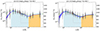 |
Fig. 4. Example of average SEDs produced employing the uncorrected (left) and corrected (right) photometry (blue). The effect of the corrections applied is to increase the flux bluewards of the Lyα and reduce the optical and UV Fe II bumps. In addition, the strong Hα emission in the observed-frame H band (pink) is reduced in the corrected data-set. The grey clouds of points are the photometric data used to produce the SED; the coloured diamonds (same colour-code as in left panel of Fig. 3) are the median luminosities. The solid grey line represents the number of objects contributing to each spectral channel. The average quasar SED from Krawczyk et al. (2013), scaled to the 3000 Å total luminosity, is shown in green as a comparison. The light blue and orange shaded areas represent the regions where the Lopt and the LNIR terms in the covering factor proxy R are respectively evaluated (see Sect. 3.5). The average z and log(Lbol) of the parameter space represented by these SEDs are denoted in the top string. |
3.5. Defining a proxy for the covering factor
The emission of the dusty torus in AGN is expected to peak between ∼3–30 μm, with noticeable differences depending on the covering factor (CF), the optical depth (τ) and the inclination of the line of sight (see e.g. Nenkova et al. 2008a; Shi et al. 2014; García-González et al. 2017). In order to precisely define the covering factor, a complete description of the SED, representing the whole accretion disc and torus emission from the extreme UV to the far infrared, is needed. Unfortunately, this is not generally feasible, especially for large samples like ours.
Several past works have adopted different infrared and UV/optical proxies, respectively, for the torus and AGN luminosity terms in the CF expression. Traditionally, the ratio R between the monochromatic luminosities at some infrared and UV/optical wavelengths (e.g. Maiolino et al. 2007; Treister et al. 2008) or integrated over the available wave bands (e.g. Cao 2005; Gu 2013; Rałowski et al. 2024) has been widely employed.
A more refined approach to the problem of evaluating the covering factor requires taking into account other factors such as the optical thickness of the torus and its shape. For instance, an optically thick torus is expected to have a lower CF (see e.g. Sect. 6 in Lusso et al. 2013). Moreover, it has been shown by Stalevski et al. (2016) that the clumpiness of the dusty torus in combination with the anisotropic emission of the accretion disc leads to the underestimation (overestimation) of low (high) CFs in type 1 AGN when adopting the bare ratio between IR and UV/optical luminosities. To correct for these effects, they propose a polynomial expansion of CF in terms of R.
The wavelengths covered by our data do not consent to properly sample the mid- and far-infrared tail of the torus emission. Similarly, the low coverage in the far-UV combined with the effect of possible residual (and redshift-dependent) IGM absorption, not completely corrected by our procedure described in Sect. 3.3.3, does not guarantee a complete description of the BBB. Because of this, we rely on observational proxies for the CF based on different combinations of UV/optical and near-infrared luminosities. Throughout this work, we adopted the ratio R = LNIR/Lopt5 as a proxy for the intrinsic CF, with LNIR being the integrated luminosity of the average SEDs between 1–5 μm and Lopt that between 1000 Å and 1 μm.
In the NIR, the WISE coverage at the redshifts sampled in this work only allows us to access the hot dust emitting in the range between roughly 1–5 μm. This spectral region can be affected by stellar emission within the host galaxy (e.g. Podigachoski et al. 2016), the infrared tail of the accretion disc, and/or sources with strong contributions by hot graphite dust (e.g. Mor et al. 2009). In our case, the selection of luminous AGN (the sample mean is log(Lbol) = 46.4 erg s−1), as well as the colour cut, help in mitigating the effect of the possible stellar light contribution. In addition, we visually inspected all the average SEDs to check that the 1 μm emission was dominated by the disc, rather than by the peak of the stellar bulge in the host, thus minimising the possible mixing of the components. On the other hand, Stalevski et al. (2016) showed that, within their model, the 1–5 μm band has the favourable aspect of having almost no dependence on the optical depth, nor on the other parameters explored therein, such as the clumpiness of the torus and the inclination angle.
For what concerns the AGN term in the CF definition we employed Lopt, defined as the integrated UV/optical BBB emission from 1000 Å emission up to 1 μm in the average SEDs, including only the bins where the peak of the disc emission was clearly observed in the data. If the UV/optical SEDs peaked at significantly different wavelengths at different redshifts and luminosities, this choice would provide unreliable results. We here rely on the evidence that the SED of quasars in different ranges of luminosity and redshift appear to universally peak around 1000 Å (see e.g. Zheng et al. 1997; Telfer et al. 2002; Shull et al. 2012; Stevans et al. 2014; Cai & Wang 2023). In Sect. 4.2 we thoroughly discuss the results obtained under these assumptions, which are the anti-correlation between R and Lbol and the non-correlation between R and z. With the aim of testing the robustness of these results we also adopted different integration limits for the disc and torus emission, and employed alternative datasets neglecting the corrections performed on the starting photometry. All the conclusions drawn for the corrected dataset, derived integrating the disc SED between 1000 Å and 1 μm and the torus SED between 1–5 μm can be extended to these alternative datasets. This is shown quantitatively in Tables 1 and 2 containing the results of the correlation analysis for the fiducial dataset, and in Table 3 for the alternative ones.
Correlation parameters between z, log(Lbol), and R.
Best-fit parameters of the relations between z, log(Lbol), and R.
Correlation parameters between z, log(Lbol), and alternative CF proxies also considering alternative datasets.
To conclude, we report that the uncertainty on R was evaluated by producing 100 mock SEDs for each object, by randomising the flux in each spectral channel adding a Gaussian deviate using the uncertainty on the final SEDs.
3.6. Reaching the rest-frame 5 μm
In this work, we limited our analysis to z < 3 so that our sample reaches a high degree of completeness at i < 19.0. This implies that the rest-frame 5 μm falls within the W3 filter up to z ∼ 2.3. Above this value, an increasing portion of the rest-frame 1–5 μm emission is sampled in the observed-frame by the W4 filter, which has been shown to be prone to overestimating the intrinsic flux when compared with instruments with similar passbands (e.g. Spitzer MIPS24, Rałowski et al. 2024). We confirmed this issue by cross-matching the W4 photometry with that of Spitzer MIPS 24 μm for a sample of common sources. In agreement with the previous findings we confirm that W4 systematically overestimates the flux in the low S/N regime. A more quantitative discussion on this issue is presented in Appendix A. Nonetheless, at z < 3 the emission between 1–5 μm is mostly covered by W1, W2, W3. In the cases where the rest-frame 5-μm emission falls redwards of the W3 filter we extrapolated the SED using the W2 and W3 photometric points using a power law. We estimated how much this prescription could underestimate the actual value of CF by performing the following exercise. We considered the average SEDs where 5 μm falls redwards of the central wavelength of W3 (12.3 μm). We assumed a typical NIR quasar spectrum represented by the template built in Hernán-Caballero et al. (2016), and matched it to the average SED at the rest-frame W3 wavelength, using it to cover the rest 5-μm emission. We then evaluated R from the template-matched and from the extrapolated SED. The typical difference is at the per cent level. We also note that this is a conservative approach, because of the actual width of the W3 filter. For instance, at 16.3 μm the filter response is still about ∼50%.
4. Results
In this Section we report the results of the analysis regarding the evolution of NIR SED and R with z, Lbol, and λEdd. Additionally, we compare the average SED built upon the whole sample with others in literature, and present how the information about the dusty torus gathered in this work can give constraints on the mechanism responsible for obscuration in the X-rays.
4.1. Evolution of the average SED with z and Lbol
A key question when trying to understand the observed properties of the obscuring torus in AGN is whether and how they change as a function of the AGN parameters (Lbol, MBH) and of the cosmic epoch. For what concerns the luminosity evolution, the sub-linear relations claimed by different authors (e.g. Maiolino et al. 2007; Ma & Wang 2013; Gu 2013) between the infrared and optical luminosities evaluated at several pairs of wavelengths, imply a relative decrease in the NIR luminosity for increasing optical and UV luminosity. This feature, as already mentioned, fits in the physical picture where the torus recedes for increasing accretion disc luminosity. From a cosmological perspective, the IR SED of high-redshift, non-dust-deficient quasars (Leipski et al. 2014) has been shown to closely resemble, on average, that of more local samples (e.g. Elvis et al. 1994; Richards et al. 2006), thus hinting at the fact that a non-evolution of the IR SED is actually possible.
Here we aim at exploring systematic changes in the shape of the NIR SED as a function of Lbol and/or z. To this end, the ideal case would be to have a uniformly populated region, as large as possible, in the parameter space. However, this is not the case for both observational and physical reasons. In any flux limited sample, the high-z and low-Lbol regions are the ones mostly affected by incompleteness. Therefore, although there might be a significant number of sources in this region, these are not probed by the surveys considered here. Conversely, the low-z and high-Lbol region is scarcely populated due to the declining number of quasars after what is known as the quasar epoch. In the next Sections, when trying to analyse the behaviour of the R ratio with Lbol and z, we define sub-regions of the parameter space which are better suited for each analysis. In each case, we aim for the best trade-off between the number of bins employed (for a more robust statistic), the dynamical range in terms of explored parameters, and the uniformity of the subset.
With the aim of understanding how the quasar SED evolves, we performed the following exercise: we considered all sources residing in the region of the parameter space comprised between 46.4 ≤ log(Lbol)≤47.4 and 1.0 ≤ z ≤ 2.8 (∼21 000 out of 36 000 quasars) and proceeded to produce composite SEDs for each luminosity or redshift bin while integrating along the other axis, following the procedure described in Sect. 3.4. Although here we pay particular attention to selecting a uniformely populated region (i.e. with a low fraction of empty bins), we note that the luminosity tends to slightly increase with redshift. For example, the average log(Lbol) at z ∼ 1.0 is 46.58, while it reaches 47.06 in the highest redshift bin at z ∼ 2.8. However, including also sources below z = 1.0, the mismatch in terms of luminosity between the low- and the high-redshift composites would be even worse, becoming as high as ∼1.5 dex.
We then employed these average SEDs (shown in Fig. 5) to test the evolution of the NIR SED shape with z and Lbol separately. We also highlight in the inset panels of Fig. 5 the values of R derived from these composite SEDs. It is easy to appreciate the relatively fainter NIR SED with increasing optical luminosity, a feature also testified by the decreasing R shown in the inset plot, despite the limited dynamical range of only one order of magnitude. The composite SEDs in z bins exhibit slightly more pronounced SED to SED variations, particularly at ∼2 μm where a turnover appears, mostly in the data at z ≲ 1.6. However, the values of R derived from these SEDs do not show any clear trend with z.
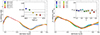 |
Fig. 5. Left: Sequence of average SEDs for increasing luminosity, scaled by their total luminosity between 1000 Å and 1 μm. The trend of decreasing NIR luminosity for increasing optical luminosity is apparent despite the small dynamical range, and it is testified by the decreasing R shown in the inset. Here the mean value (standard deviation) is shown as a black solid (dashed) line. Right: Sequence of average SEDs for increasing redshift, scaled by their total luminosity between 1000 Å and 1 μm. The different sampling of the rest-frame emission leads to slightly different SEDs. However, on average R does not show any evolutionary trend as we do not observe systematic departures from the mean value. |
An interesting feature is the slight change of position of the 1 μm dip. This dip results from the combination of the low-energy tail of the emission from the accretion disc and the rise of the emission from the innermost region of the torus. Small changes in the position of this feature can be observed in both panels of Fig. 5. This is mostly caused by the different contributions of the disc and the hot torus components, chiefly affecting the SEDs at different Lbol. It can be easily shown that the combination of an increasingly more luminous accretion disc with a relatively fainter torus in its innermost hottest region, produces a shift towards longer wavelengths of the dip.
Another relevant detail is that producing average SEDs in different fixed redshift bins introduces the technical issue given by the uneven sampling of the rest-frame spectrum, which, in the NIR, is exacerbated by two factors: the first is the scarce sampling due to the presence of only the three WISE filters (W1, W2, W3), and the second is the non-power law shape of the continuum. The combination of these factors leads to the seeming differences in the NIR of the average SEDs at different z as we show in Appendix B. However, such effect is not present in the SEDs at fixed luminosity where, instead, the wide range of redshifts allows for a finer sampling of the rest-frame spectra.
With the end of verifying whether the SEDs in bins of fixed z are consistent with an intrinsically constant NIR SED not varying with the redshift, we performed an additional test: we created an intrinsic FUV-to-NIR SED by joining three spectral templates, namely the Zheng et al. (1997) template for the FUV, the Selsing et al. (2016) for the UV and optical, and the Hernán-Caballero et al. (2016) for the NIR. The choice of the Selsing et al. (2016) template, rather than the Vanden Berk (2001) one, was mainly driven by the fact that the former is based on luminous quasars, hence the optical band is almost unaffected by the host galaxy, as expected for the objects in the subsample considered here. In this case we opted for a NIR spectral template, rather than a photometric SED, in order to include the effect of the emission lines at different z, as we did not subtract NIR emission line features from our photometric dataset. As done for each of the sources in the parent sample, we removed the contribution from prominent broad emission lines, as well as the UV and optical Fe II pseudo-continua. We then shifted the spectral template to the same redshifts where the average SEDs had been produced, and convolved it with the filters of the surveys employed in this work. Lastly, we evaluated R in the same way as it was estimated from the actual SEDs. In the cases where the observed-frame photometry did not cover the rest-frame 5 μm, we resorted to extrapolation. The result of this further test is shown in Fig. 6. Here we highlight two noticeable features: the first is that the turnover at ∼2 μm, present in the composite SEDs below z ∼ 1.6, is also observed in the simulated SEDs at the same redshift, where both the rising and the flat regions of the NIR bump (consistent with a blackbody emission at T ∼ 1200 K, Hernán-Caballero et al. 2016) are sampled by W1, W2, and W3. As the redshift increases, only the rising part of this bump is sampled by the WISE filters, hence the power-law extrapolation. This effect is shown in detail in Appendix B, where we demonstrate how the interpolation (and extrapolation) across the filters of the template varies with the redshift. Secondly, we note that, although R is slightly different in absolute value with respect to that observed in the actual data6, it does not show any conspicuous trend, notwithstanding the different sampling wave bands. The dispersion in R is close to consistency with a single NIR SED at all redshifts: the standard deviation of R estimated in the simulated SEDs (0.012) is indeed remarkably similar to that of actual SEDs (0.014), thus leaving little room for further effects causing the observed dispersion. As a comparison term, the standard deviation of R at different Lbol reaches 0.020 in just one order of magnitude, while also showing an obvious decreasing trend (see the inset plot of the left panel in Fig. 6). Additionally, this sampling effect on the same quasar SED at different redshifts causes the dip to move, as we show in Appendix B, thus adding up to the already mentioned luminosity effect.
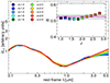 |
Fig. 6. Composite SEDs from the simulated photometry of the template in the same redshift bins of the actual data. Here the magenta line marks the actual R value estimated using the total spectral template rather than the photometry. |
To sum up, the average SEDs produced at fixed Lbol confirm the trend of a weaker NIR emission for increasing optical luminosity. This is clearly observed even employing a relatively small dynamical range (1 dex). We also argue that, despite some SED-to-SED variations, the average SEDs at different z are consistent with an intrinsically similar rest-frame NIR SED sampled at different observed-frame wave bands, rather than with an actual evolution with z. There are obviously other effects, here not taken into account, which might contribute to the SED-to-SED differences. For instance, in the real data, the average luminosity increases slightly in each redshift bin, as already noted, therefore influencing the NIR emission accordingly. Furthermore, the differences in luminosity are likely accompanied by minor changes in the emission line strength, which are not taken into account by our fixed NIR template.
4.2. Analysis of the correlation between CF, Lbol and z
The evolution of the NIR SEDs with Lbol can be epitomised in the (sub-linear) anti-correlation between the CF and the AGN luminosity. The fraction of the solid angle covered by the obscuring torus diminishes for increasing luminosity. Here we aim at quantifying the respective effects of the luminosity and redshift in driving the evolution of CF.
The main axes of our parameter space (i.e. the bolometric luminosity and the redshift) are correlated for both physical and observational reasons. More luminous AGN, or quasars, are generally observed at redshifts corresponding to the quasar epoch at z ∼ 2 − 3. At the same time, being the SDSS a flux limited survey, faint objects at increasingly larger distances do not reach the flux limit. We therefore aimed at employing statistical tools to assess the degree of correlation between our proxies of the CF and the main parameters that could account for this effect. In particular, we adopted a methodology similar to that used in Croom et al. (2002), who studied the independent effects of luminosity and redshift on the evolution of the equivalent width of broad and narrow emission in the quasar population. There, the authors used both a partial correlation analysis (PCA, which we introduce below), and performed linear fits between the parameter of interest and the equivalent width, while keeping the other fixed.
The first approach in this analysis was to estimate the degree of correlation between R and the main parameters via a PCA. This tool allows us to disjointly evaluate the degree of correlation between R and one of the main parameters, while keeping the other fixed (see e.g. Bluck et al. 2022; Baker et al. 2023). This kind of analysis requires a monotonic dependence of R on both the main parameters. This is the case for the log(Lbol)−R relation, while the correlation between R and z appears weaker, as also testified by the correlation indices explored below. In particular, given the three or more quantities (A, B, C) we wish to test the correlation on, the partial correlation coefficient between A and B while keeping C fixed can be expressed as:
where ρXY denotes the Spearman rank correlation index between quantity X and Y. We used the PCA values to define a gradient arrow in Fig. 7, whose inclination is defined as:
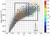 |
Fig. 7. log(Lbol)–z plane with R shown as coloured dots (see colour bar at right). The black arrow points in the direction given by the PCA, evaluated in the bins within the black rectangle, while the dashed arrows show the uncertainty on the direction. The coloured rectangles highlight the bins of the parameter space shown in Fig. 8. We recall that the bins between 46.4 ≤ log(Lbol)≤47.4 and 1.0 ≤ z ≤ 2.8 are included in the SED evolution analysis described in Sect. 4.1. |
The arrow shows the direction of strongest variation in the tested parameter. The more aligned the arrow with an axis, the stronger the correlation with that quantity. The PCA arrow is almost completely (θ = −86°) inclined towards decreasing log Lbol values, signifying that the increasing bolometric luminosity is ultimately responsible for the decrease in the covering factor. We performed this analysis in the region marked by a thick black rectangle in Fig. 7, which is made of 56 bins with more than 30 sources per bin. This choice avoids the low-luminosity tail at redshift below z = 0.7, where R reaches its maximum values. We opted for this choice in order to avoid regions of the parameter space where galaxy contamination is expected to be ≳10%. We note, however, that the inclusion of the few bins below log Lbol = 46.0 would not alter any of the results presented here. Additionally, we tested whether the decrease in R could be due to decreasing host contamination with increasing Lbol using the emission-line subtracted template described in Sect. 4.1. The decrease in R starting from a 10% galaxy to a totally quasar-dominated emission at 5100 Å is of the order of 5%, incompatible with the ∼30% decrease observed in the selected bins.
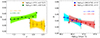 |
Fig. 8. z–R (left panel) and log(Lbol)–R (right panel) section of the parameter space for the bins denoted by rectangles with the same colour-coding in Fig. 7. The solid lines represent the best linear fits to the data, while the shaded areas, obtained by resampling the posterior distributions of the best fit parameters, mark the 95% confidence intervals. |
We also evaluated the uncertainty on this parameter via a bootstrap resampling of the values of R. We computed θ 1000 times, each time using a random subsample made of only 30/56 bins in the PCA region, allowing for re-immission. The uncertainty on the PCA inclination was evaluated as the standard deviation of the distribution of ∣θ∣. For the sake of completeness we also report in Table 1 the partial correlation coefficients and the respective p-values associated to the null hypothesis that there is no correlation between the variables. In Fig. 7 we show R derived from the SED in each bin of our parameter space in colour-code superimposed to the whole sample. We also plot the arrow representing the main direction of the PCA, which clearly indicates Lbol as the main driver of the evolution of R.
As a further test, we also employed a similar procedure based on the use the Kendall τ index of correlation (Kendall 1938) instead of the Spearman one, as it provides more robust results in the case of outliers. The partial correlation evaluated using the Kendall τ has the same form highlighted in Eq. 4 with ρ replaced by τ (Akritas & Siebert 1996). In this case, we adopted a permutation test to compute the associated p-value (see e.g. Tibshirani & Efron 1993). In brief, given three or more quantities we wish to test the correlation on (A, B, C), we shuffle the array containing the parameter A, to simulate a non-correlation (random association) between both the A-B and A-C pairs, while keeping the relation between B and C unaltered. Then, we proceed to evaluate the partial correlation coefficient τAB ∣ C for this simulated dataset. This procedure is repeated 10 000 times, producing the test distribution, and the p-value is estimated as the two-tailed fraction of simulated datasets where τAB ∣ C exceeds the observed value. The resulting values for our dataset are reported in Table 1. We also employed these correlation coefficients to estimate the inclination of the PCA arrow, finding a consistent result (−80°).
Additionally, as another independent check on the correlation strength, we performed the regression of linear forms between R and one of the two parameters, while keeping the other fixed. Again, this was performed in the rows or columns of the parameter space within the same region where the PCA was evaluated. In more detail, we adopted the functional forms as:

![$$ \begin{aligned} ii) \,\, R&= a_0 + a_1 \, [\log (L_{\rm bol}) - L_0], \end{aligned} $$](/articles/aa/full_html/2025/05/aa52609-24/aa52609-24-eq11.gif)
respectively for the R − z and the R − log(Lbol) relations, with z0 and L0 being the mean of the z or log(Lbol) values upon which the regression was performed. In this case the slope of the line gives information about the strength of the correlation between R and any of the two parameters while keeping the other fixed. We report the average slopes and offsets of the best-fit relations in Table 2. We remark that both the relations are merely empirical efforts to describe the correlation between the parameters of our space and the proxy that we adopted for the actual covering factor. These results are used as statistical tools of comparison, while a physical description of the evolution of the covering factor with any of these parameters would require a detailed modelling, beyond the scope of this work.
In Fig. 8 we show, as an example, the z − R and the log(Lbol)−R projections of the parameter space highlighted as rectangles in Fig. 7, together with the best-fit relations.
In general, the partial correlation coefficients clearly indicate Lbol as the main driver of the correlation (ρ = −0.770, p-value = 6.4 × 10⁻¹², τ = −0.563, p-value < 10−4), while at fixed luminosity z plays no role in the evolution of R (ρ = 0.057, p-value = 0.678, τ = −0.099, p-value = 0.219). The same finding is testified by the average slopes of the linear regressions: the anti-correlation between Lbol and R is systematically detected at all redshifts with the average slope of the linear regressions of ⟨a1, L⟩= − 0.055 ± 0.012. On the other hand, the average slope of the z − R relation is consistent with zero within ∼1σ, being ⟨a1, z⟩= − 0.008 ± 0.007.
The selection of 5 μm as the longest wavelength to sample the torus emission was chiefly dictated by the trade-off between choosing a wavelength well within the IR regime and the maximal observability throughout the sample. At the same time, the choice of employing the ratio LNIR/Lopt, evaluated respectively between 1–5 μm and 1000 Å–1 μm, as a proxy for the intrinsic CF was mainly due to our data-driven approach. As consistency checks, we performed the same analyses described in the previous Section adopting different proxies for the CF and alternative datasets.
-
We explored the adoption of the 2–5 μm interval for estimating the IR term contained in R (subset R2−5 μm in Table 3). A longer wavelength for the lower end of the IR term is more reliable when it comes to estimate the torus emission, being less prone to possible stellar emission within the host galaxy. The price for this choice is, however, the narrowing of the integration interval and the consequent lowering of the R value.
-
We explored the possibility of integrating the accretion disc SED between its peak and 1 μm rather than in the fixed 1000 Å–1 μm interval (subset Rpeak − 1 μm).
-
With the aim of taking into account the effect of the anisotropy of the accretion disc radiation field, as well as the clumpiness of the torus, we tested the parametrisation described in Stalevski et al. (2016). To this end, we scaled R to the total ratio between the 1–1000 μm infrared luminosity and the disc luminosity (see Section 4.6 for more details, subset CFS16).
-
We also explored the CF the expression described in Lusso et al. (2013), CF = R/(1 + (1 − p)R), where the p parameter takes into account the optical depth of the torus to its own radiation. An optically thin torus has p = 0, whereas an optically thick torus has p = 1 (subset RL13).
-
As additional checks to make sure that the corrections made to the photometry, as well as the colour selection criterion, have not altered the results, we also present the same results obtained without including these corrections (respectively the subsets “no-corr” and “no-col”).
The results evaluated adopting these alternative prescriptions and datasets are shown in Table 3. The structure of the table is the same as that of Tables 1 and 2.
Although the absolute value of the CF proxy obviously depends on the parametrisation and the wavelength interval for the LNIR and Lopt terms, the trends described in the main text are confirmed adopting all the other possible choices. In the dataset where the 2–5 μm interval was adopted a significant correlation appears between R and z according to the Spearman index. However, this trend is neither confirmed by the Kendall correlation index, nor by the average slope of the fitted regression lines.
To conclude, these results suggest that the covering factor, here parametrised by its proxy R, does not evolve with redshift, and its evolution is only driven by the AGN luminosity. A direct consequence of this finding, to which we return in the discussion, is the self-similarity of the innermost region of the AGN throughout cosmic time, at fixed luminosity.
4.3. The full-sample SED
In Fig. 9 we show the comparison between the SED obtained using our full sample and other SED templates in the literature (Krawczyk et al. 2013; Saccheo et al. 2023). Additionally, we show in black the spectral composite from Euclid Collaboration: Lusso et al. (2024) to compare our photometry to Euclid NIR spectroscopy. Lastly, we also present the average SED of a control sample of sources observed in the Stripe 82 (S82, Annis et al. 2014) whose properties are discussed more in detail in Sect. 4.6.
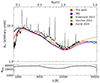 |
Fig. 9. Our full-sample SED and others from literature (see text). All the SEDs are normalised by their integrated luminosity between 1000 Å and 1 μm. The AGN spectral composite from Euclid Collaboration: Lusso et al. (2024) is scaled to match our SED (red solid line) at 2200 Å. The black line in the bottom panel shows the number of sources contributing per spectral channel in the average SED. The full-sample composite SED is available in its entirety in machine-readable form in the online journal. |
The SEDs are scaled by their integrated luminosity between 1000 Å and 1 μm for a proper comparison. In the optical, our global SED resembles that from Krawczyk et al. (2013) and the S82 control sample, as expected since also these works were based on SDSS samples. In the range between 5000 Å–1 μm the Krawczyk et al. (2013) SED exhibits some excess with respect to ours, likely due to minor galaxy contamination. Their sample is indeed roughly one order of magnitude deeper (see the dashed line in their Fig. 2, marking the SDSS DR7 luminosity threshold), and therefore more incline to a higher fraction of host galaxy light in the optical/NIR. In the IR, the average SED from Saccheo et al. (2023) outshines the SDSS-based samples, again unsurprisingly, being these quasars IR-selected. The small blue bump associated with the Fe II UV pseudo-continuum between 2250–3300 Å (e.g. Grandi 1982), visible in the other average SEDs, instead appears to have been well subtracted in ours.
4.4. Evolution of CF with the Eddington ratio
The Eddington ratio expresses the efficiency of the accretion process in AGN, with sources emitting close or above the Eddington limit having reached their maximal radiative emission under the assumption of spherical accretion. Despite this simplistic approximation, this parameter represents a reasonable proxy for the normalised accretion rate. By scaling the emitted luminosity by the black hole mass (which sets the black hole sphere of influence), the Eddington ratio is a “scale invariant” quantity, in contrast with the bare Lbol. Tori with similar covering factors possibly share similar accretion properties (see e.g. Ricci et al. 2023, and references therein).
With the aim of investigating this possibility, we explored the evolution of the covering factor within the accretion parameter space (i.e. the parameter space given by log(MBH) and log(Lbol))7. Since we just showed that the seeming dependence of the covering factor on z actually derives from the effect of the luminosity, here we do not take into account any redshift effect. For this analysis, we basically repeated the same steps adopted to build the log(Lbol)–z parameter space, keeping the same binning width. We then proceeded to produce the average SEDs and evaluate R accordingly. We also computed in each bin the average λEdd. This alternative parameter space, together with the R parameter in colour-code, is shown in Fig. 10. The standard correlation indices (i.e. not partial) for the log(Lbol)–R and the log(λEdd)–R relations confirm, as expected, the presence of significant correlations for both the relations. In particular, we report ρ = −0.905 for log(Lbol)–R, with p-value < 10−20, and ρ = −0.497 for log(λEdd)–R, with p-value = 3 × 10⁻⁵. Although both anti-correlations are statistically significant, the face values suggest that the stronger driver of the two, in the evolution of the covering factor, is the luminosity. We reached an equivalent result by employing the τ index of correlation, which gives τ = −0.733 (p-value = 6 × 10⁻¹⁸) and τ = −0.363 (p-value = 2 × 10⁻⁵), respectively, for Lbol–R and λEdd–R. A more informative way to tackle this question is to perform again a PCA, this time within the accretion parameter space, and check a posteriori the direction of the strongest correlation. We performed this test on the bins residing in the region mostly uniformly populated, marked as a black rectangle in Fig. 10. As described in Sect. 4.2, we evaluated the PCA between log(Lbol) and R, while keeping log(MBH) fixed, and vice-versa. We also evaluated the uncertainty on the direction of the strongest correlation by performing a bootstrap resampling. The PCA arrow aligns almost completely (θ = −80°) with the direction of decreasing log(Lbol). The relative intensity of log(Lbol) is still dominant when evaluating the correlation using the τ index, giving θ = −86°. In Fig. 10 we show the PCA direction of increasing R as a black arrow. As a comparison, we also mark as a magenta arrow the direction of decreasing λEdd, which should be followed by an increase in the covering factor if the Eddington ratio were the main driver of the CF evolution. Clearly, the effect of Lbol is stronger than that of the Eddington ratio in driving the evolution of CF.
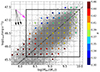 |
Fig. 10. log(MBH)–log(Lbol) plane, with R shown as coloured dots (see colour bar at right). The black rectangle shows the region where the PCA was evaluated. The black solid and dotted arrows represent the direction of the strongest correlation as in Fig. 7. The dash-dotted line marks a constant λEdd = 0.2, representing the average value of the sample, while the magenta arrow shows the direction expected if the increase in R were driven uniquely by the decrease in λEdd. |
Again, Lbol appears as the main driver in the evolution of CF. However, cannot exclude that an intrinsically tighter correlation exists between CF and λEdd, which is observationally diluted because of the large systematic uncertainties on the black hole masses of the current calibrations (0.3–0.5 dex, see e.g. Vestergaard & Peterson 2006).
4.5. Accounting for selection effects
As we have thoroughly discussed, one of main results of this work is the assessment of any possible evolution of CF with z. Since we built this sample starting from the cross-match of flux-limited surveys, it is extremely important to take into account to what extent selection effects can affect our results. These can come basically in two forms: incompleteness and inclination. The first effect is produced whenever the optical detection is not matched by the IR counterpart in a substantial fraction of objects. This implies that only the most IR-bright objects are selected because of the IR flux sensitivity, thus biasing the CF towards higher-than-average values. In our case this issue is not critical since, as we already mentioned, the IR-to-optical cross-match fraction (∼97%) guarantees a high degree of completeness with respect to the optical survey, which also claims to be ∼90% complete.
The second effect has a subtler impact on the observations. It is generally assumed that the optical/UV emission comes from an accretion disc, while the IR radiation is isotropically emitted by the torus (see e.g. Treister & Urry 2006 and references therein). In flux-limited surveys, at higher redshifts increasingly fainter objects fall below the flux limit of the survey. Assuming that the intrinsic luminosity is diminished because of the projection effect as Lbol, obs = Lbol, int cos θ, with θ being the angle between the line of sight and the axis of the accretion disc, the same observed luminosity can be obtained by intrinsically brighter sources observed at higher inclination or vice-versa. Even assuming that all the quasars in the Universe had the same intrinsic luminosity (which is obviously not true) and random inclinations of the line of sight, the combined effect of the flux limit and the increasing distance with z would imply the selection of preferentially face-on objects. This, in turn translates into a relatively higher contribution of the optical/UV with respect to the IR (i.e. lower CF) for increasing z.
Such an effect would produce an anti-correlation between the CF and z at a given intrinsic luminosity, but in the following we demonstrate that, within the ranges of parameters explored in this work, it does not produce any statistically appreciable trend. Another, likely overly fine-tuned possibility is that the effect of increasingly face-on objects combines with intrinsically higher CF so that the two effects cancel out. Similarly, the anti-correlation observed in the dataset between between CF and Lbol at constant z (see Sects. 4.1, 4.2), under the reasonable assumption of random inclinations of the line of sight at the same redshift, cannot be ascribed to inclination effects. Therefore, the widely discussed anti-correlation between CF and Lbol that we observe is likely a genuine feature rather than one induced by observational effects.
To quantify the impact of the inclination angle at increasing redshifts on the observed CF we took advantage of a simulation. The basic idea here is to simulate a population of quasars whose intrinsic bolometric luminosity and covering factor distribution are known and see how the effect of inclination and flux limit propagate in the observed CF in the parameter space defined by Lbol and z. To this end, we produced a mock sample of 100 000 objects uniformly distributed in the parameter space. The limits of the z and log(Lbol) distributions overlap with those spanned by the actual sample: z = [0.1, 2.9] and log(Lbol) = 45.0–48.5; the upper limit of the luminosity was chosen to be slightly higher so as to include very luminous, but inclined objects. We assumed a normal intrinsic CF distribution with mean value ⟨CF⟩ = 0.5 and standard deviation σCF = 0.05, with the underlying assumption that there is no physical connection between the torus CF and the AGN luminosity. For each object we draw a random value of cos θ from a uniform distribution between [cos 0° , cos 90°], representing random line of sights to the AGN of the sample, and derived the projected bolometric luminosity accordingly. This allowed us to produce the observed CFobs = CF/cos θ.
Successively, we produced the simulated photometry by assuming a 3000 Å luminosity L3000 Å = Lbol/5.15 from the bolometric corrections of Richards et al. (2006) and matching a quasar template (Vanden Berk 2001) to L3000 Å. Finally, we discarded all the objects whose i photometry fell above mi ≥ 19.0 (the magnitude limit chosen for this work, see Sect. 2) and whose inclination angle was above 65°, assuming an infinitely optically thick torus. Above this level of inclination, the broad lines would not be detected and the optical/UV SED would not exhibit the blue colours of unobscured quasars, and the source would be consequently excluded from the survey.
In Fig. 11 we show the result of this procedure. There are several details to be noted here: the first and foremost is that the combined effects of inclination and flux limit are not capable of producing any appreciable trend in the two dimensions of the parameter space. Secondly, we note that the average observed covering factor CFobs is ∼0.7, while the intrinsic one set in the simulation was CF = 0.5. This can be explained as the effect of the average inclination by which CFobs = CF/⟨cos θ⟩≃CF/0.7 ≃ 0.7. Lastly, we see that the data in the brightest bin hint at a tentative decrease in CF. This is because the most luminous objects in the distribution cannot be interpreted in terms of some even more luminous sources observed under high viewing angles. In this tail of the distribution, the observed luminosity is close to the intrinsic one, and CFobs tends to CF. We also explored other combinations for the simulation parameters within reasonable values, but in no case we managed to obtain any clear trend.
 |
Fig. 11. z–CF (left) and log(Lbol)–CF (right) section of the simulated parameter space. The CF and log(Lbol) values presented here are the observed (i.e. projected) quantities. The magenta diamonds represent the median CF values in bins of 0.2 dex in width. The y-axis uncertainties represent the standard error on the mean CF in the bin. The third axis is colour-coded. |
There are obviously several over-simplifications in this approach, such as the flux limit selection, which is much more complex than a bare magnitude cut. The assumption of a completely optically thick torus is also at odds with the patchy torus models, which admit a non-zero probability of seeing directly through the torus. Lastly, the isotropic and perfectly efficient re-irradiation of the primary continuum by the torus in the infrared is another very simplistic zero-th order assumption. However, the lack of a clear decreasing trend, especially in the moderate- to high-luminosity regime, is reassuring for what concerns the robustness of the correlation between the CF of the torus and the disc emission.
4.6. The non-evolution with z of the torus in AGN: implications for the X-ray obscured fraction
The analyses carried out so far strongly suggest a non-evolution with z of the torus properties, at least in its innermost region for the blue, type 1 AGN included in this sample. When this evidence is coupled with the seeming non-evolution of the optical/UV SED between local and high redshift-quasars, it appears that the nuclear structure in blue quasars only depends on the luminosity of the nucleus, regardless of the cosmic epoch. Within the unified model, a redshift-independent torus geometry translates into a constant fraction of optical type 1 AGN at fixed luminosity (see e.g. Fig. 6 in Merloni 2003) at all cosmic times. As an application of this result, we can employ the covering factor derived from LNIR/Lopt to set a lower limit for the X-ray obscuration. X-ray obscuration can be indeed produced on different scales (nuclear/circumnuclear and galactic), and by dusty and/or dust-free gas. If the amount of obscuration imparted by the torus does not vary with redshift, any kind of evolution in the obscuring medium should occur elsewhere.
We thus aimed at comparing the covering factor here derived via the LNIR/Lopt ratio with that estimated in several X-ray surveys. We achieved this by converting our proxy into the actual covering factor adopting standard prescriptions. In particular, we show that, adopting reasonable assumptions regarding the disc emission and the torus opening angle, it is possible to reproduce the X-ray obscured fraction at z ∼ 0, and set a lower limit for the X-ray obscuration.
We show the result of this approach in Fig. 12. There, we present the evolution with the redshift of the fraction of X-ray obscured objects (with column density NH > 1022 cm−2) according to different literature samples (Aird et al. 2015; Buchner et al. 2015; Ananna et al. 2019; Peca et al. 2023). When the AGN sample included only Compton-thin objects, we adjusted the obscured AGN fractions by assuming an equal number of Compton-thin and Compton-thick sources (e.g. Gilli et al. 2007; Ananna et al. 2019). The samples presented here are in the X-ray luminosity regime LX ∼ 1045 erg s−1. The obscured fractions of the reference samples were corrected for the effect of the Malmquist bias, which reduces the fraction of observed obscured sources, by assuming intrinsically equal amounts of obscured and unobscured sources (i.e. p = 0.5 in Eq. (1) in Signorini et al. 2023).
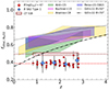 |
Fig. 12. Obscured AGN fraction with NH > 1022 cm−2 as a function of redshift in different literature samples (Aird et al. 2015; Buchner et al. 2015; Ananna et al. 2019; Peca et al. 2023), including a correction for Compton-thick sources (see text for details). The data derived from the sources at log(Lbol)∼47 in our sample are shown as red dots. The S82 quasars in the same luminosity range exhibit similar values of R. The hollow rectangle shows the values covered by the CF derived according to the Stalevski et al. (2016) prescription. The average of the measured values and the inferred values are both extrapolated at the redshifts not directly covered by our bins at log(Lbol)∼47 as shown by the dashed lines. The black dotted and dash-dotted lines correspond to the Gilli et al. (2022) models for δ = 3.3, γ = 2.0, and, respectively, θ = 50° and 70°. |
To assess the degree of obscuration ascribable to the torus and compare it with other samples in literature, we matched the X-ray luminosity by selecting all the bins in the log(Lbol)−z plane between 46.5 ≤ log(Lbol)≤47.5 and 0.9 ≤ z ≤ 2.9. This bolometric luminosity range fairly matches the X-ray one adopting the Duras et al. (2020) X-ray to bolometric conversion. This region of the parameter space is densely populated and allows us to sample a wide redshift interval also covered by the X-ray samples.
We proceeded by converting the observed R = LNIR/Lopt into the actual covering factor CF. We accounted for the anisotropy of the disc emission and the clumpiness of the torus by employing the Stalevski et al. (2016) prescriptions to evaluate CF. Since the covering factor is defined on the basis of the ratio between the total torus and disc luminosities, we needed to scale the observed quantities derived on smaller wavelengths ranges into the total luminosities. We achieved this by following this procedure. For what concerns the disc emission, with the aim of a consistent treatment, we adopted the same parametrisation described in Stalevski et al. (2016) (see their Eq. (2)). We used this this analytical SED to define the scaling factor to be applied to the Lopt already computed to convert this quantity into a total disc luminosity between 10 Å and 1 μm. We performed a similar exercise to take into account the far-infrared (FIR) emission from the torus. Here, we assumed the infrared emission to be well described by the intrinsic (i.e. subtracted from star formation emission) type 1 template described in Lyu & Rieke (2017). We then proceeded to compute the total torus luminosity between 1 μm and 100 μm, and used this quantity to scale the observed NIR luminosity which is instead integrated between and 1–5 μm.
Lastly, we employed the total disc and torus luminosities to evaluate CF adopting the Stalevski et al. (2016) polynomial (see their Table 1, row τ9.7 = 5). The interval covered by the values derived in this way is shown as a hollow maroon rectangle in Fig. 12. Interestingly, the CF values derived following this procedure are close to CF ≃ 0.5, and therefore manage to nicely reproduce the loose constrains coming from the extrapolations of the X-ray obscured fractions at low z.
The information collected about the evolution of X-ray obscuration in these samples should not be directly extrapolated to our sample, unless we have solid reasons to believe that their broadband properties are similar to ours. In order to verify this point, we directly repeated the whole process to derive the average SEDs for the sample described in Peca et al. (2023), which is largest sample targeted by these X-ray surveys. The latter work presents a catalogue with a detailed spectroscopic X-ray analysis of the sources residing in the SDSS Stripe 82, therefore offering a multi-wavelength description of the nuclear environment in these sources. To build the average SEDs we started by cross-matching the Peca et al. (2023) catalogue with the SDSS DR16 adopting a 3.0″ matching radius, in order to select only spectroscopically confirmed type 1 quasars, which amount to ∼48% of the starting sample. Additionally, we applied the already mentioned colour cut to exclude objects possibly affected by reddening. We then proceeded to gather all the available photometry and produce the average SEDs following the same procedure as in Sect. 3.4 for sources in the same luminosity range as those presented in Fig. 12, which is 4.65 ≤ log(Lbol) ≤ 47.5. The average UV-to-NIR properties of this sample are fairly similar to those of our main sample, as it is clear from the comparison of the global SEDs in Fig. 9. In order to assess the possible evolution with the redshift of the R ratio in the S82 sample, we also produced average SEDs in redshift bins with width Δz = 0.5 between z = 1.0 and z = 3.0 (blue crosses in Fig. 12). We found that the R values estimated in these bins largely overlap with those of our main sample (red dots), without any clear trend with the redshift. The similarity in terms of SED shape, as well as the absence of an evolution of R with z as observed also in our main sample, make us confident about the fact that the average X-ray properties derived for the S82 sample are similar to those of the bulk of our sources.
In Fig. 12 are also highlighted the curves from the analytical model described in Gilli et al. (2022) accounting for both the ISM and the torus absorption in the X-rays, corresponding to δ = 3.3, γ = 2.0, and θ = 50° (black dotted line), and θ = 70° (black dash-dotted line), which encompass the possible range of CF values. Here δ is the exponent in the relation between the column density (NH) and z (i.e. NH ∝ (1 + z)δ), γ is the exponent in the relation describing the evolution of the surface density of the molecular clouds (Σ) with z, that is Σ ∝ (1 + z)γ, and θ is the torus half-opening angle evaluated from its vertical axis. We also display the LNIR/Lopt ratios (red dots) and the derived CF according to the Stalevski et al. (2016) recipe (maroon rectangle). The lines guide the eye at the redshifts not actually sampled by the Lbol ∼ 1047 erg s−1 bins.
The model curves, assuming a plausible range of opening angles, manage to reproduce the X-ray obscured fraction, which at z = 0 can be explained by the torus alone. The resulting opening angles implied by the model are consistent with other independent estimates derived from modelling the infrared emission in type 1 AGN (e.g. Ramos Almeida et al. 2011; Ichikawa et al. 2015). Interestingly, also studies not directly aimed at investigating the torus properties provided evidence for similar values. For instance, Signorini et al. (2024), while attempting to explain the remarkably small intrinsic dispersion of the X-ray to UV luminosity relation in quasars, found – in a completely independent way – the need for the presence of a toroidal structure obscuring the accretion disc with an half opening angle ≲65° from the disc axis.
The covering factors estimated by converting the infrared-to-optical ratios manage to reproduce the extrapolation of obscured fraction at low z. However, while the obscured fraction appears to increase with z, as we already discussed, the CF is fairly constant with redshift. The increase in the X-ray obscured fraction with z calls for some sort of redshift-dependent absorber. However, the nature of this additional component is not clear, nor are the scales where the absorption of the X-rays should happen. In principle, an increase in dust-free gas in the micro-scale (i.e. the BLR) and/or dust and gas in the macro-scale (i.e. the ISM scale) towards earlier cosmic times could go in the direction of bridging the gap between the degree of obscuration derived in optical/infrared and X-ray surveys.
5. Discussion
Understanding the evolution of the covering factor and its dependence on the parameters regulating the accretion process is a crucial step towards revealing the complicated and dynamic structure of AGN. In this effort, valuable information can be gathered by exploring the broadband correlations between the primary emission from the accretion disc and the reprocessed emission by the dusty torus in the infrared. The large photometric dataset presented here, spanning roughly two and a half orders of magnitude in terms of bolometric luminosity, has been purposefully assembled to explore these correlations up to z ∼ 3, when the Universe was about 2 Gyr old.
Here, we showed that the disc luminosity acts as the main driver in the evolution of the NIR properties in our sample, representative of blue unobscured type 1 AGN. This results in an anti-correlation between the AGN luminosity and the torus covering factor, here parametrised via the ratio R between the NIR and the UV/optical luminosity. Conversely, the redshift does not play a significant role, as the CF does not evolve between low- and high-z objects at fixed luminosity.
The large sample analysed in this work provides compelling evidence against a redshift evolution of the dusty torus geometry, at least in its innermost, hottest region. The NIR SED, once we control for the dependence on the luminosity and take into account the effect of the shifting wavebands, does not exhibit any evolution with z. The most likely driver in the covering factor appears to be the AGN luminosity, whose intensity directly shapes the circumnuclear surroundings. In a broader perspective, the similarity of the SEDs between low- and high-redshift quasars is remarkable. The optical/UV SED of blue unobscured AGN are barely sensitive to the passing of cosmic time since z ∼ 7 (e.g. Kuhn et al. 2001; Mortlock et al. 2011; Hao et al. 2013; Shen et al. 2019; Yang et al. 2021; Trefoloni et al. 2024b). Similar considerations apply to the interplay between the accretion disc and the X-ray coronal emission. Their coupling, epitomised in the LX − LUV relation (Tananbaum et al. 1979), does not exhibit any appreciable redshift evolution up to z ∼ 7 (Lusso et al. 2015; Risaliti & Lusso 2019; Salvestrini et al. 2019; Nardini et al. 2019; Lusso et al. 2020) once observational biases have been removed. The similarity between low- and high-redshift quasars also holds in terms of broad emission line properties. Several works investigating the evolution of the broad lines in large samples of quasars have indeed demonstrated the absence of significant redshift trends at fixed luminosity (Croom et al. 2002; Nagao et al. 2006; Stepney et al. 2023). Analogue results have been obtained when investigating the chemical enrichment of the BLR, parametrised, for instance, via the UV Fe II to Mg II λ2798 or the optical Fe II to Hβ ratios, which do not evolve up to z ∼ 7 (Dietrich et al. 2003; Mazzucchelli et al. 2017; Sameshima et al. 2020; Wang et al. 2022; Trefoloni et al. 2023; Jiang et al. 2024; Trefoloni et al. 2024a). Putting together these pieces of evidence, what follows is that the quasar nuclear environment (i.e. the ensemble made of corona, accretion disc, BLR, and torus) is barely sensitive to the redshift, once the accretion parameters are fixed. The striking similarity between high- and low-redshift AGN goes in the direction of an early assembly of the nuclear region in luminous AGN, with the BLR of high-redshift quasars being already enriched by z ∼ 7 and the circumnuclear torus shaped according to the quasar radiation field.
A direct comparison with other works exploring the correlations between the CF and the accretion parameters is not straightforward. There are indeed several technical limitations on the available wavebands at different redshifts, as well as different proxies adopted in literature to estimate the covering factor. For instance, earlier works on PG quasars (Cao 2005) adopted the 3–10 μm interval to estimate LNIR, while both Gu (2013) and Rałowski et al. (2024) adopted the 1–7 μm interval and, more recently, Wu et al. (2023) took advantage of the 1–10 μm band. Conversely, Lusso et al. (2013) and Ichikawa et al. (2019) performed an SED decomposition first, and then integrated the best-fit torus model between 1–1000 μm. Similar considerations apply to the choice of Lopt. Despite these minor differences in the adopted proxies of the covering factor, our results follow the trend generally observed in studies using LNIR/Lopt as a proxy of CF, which find an anti-correlation between CF and both the disc luminosity and the Eddington ratio (Treister et al. 2008; Maiolino et al. 2007; Calderone et al. 2012; Ma & Wang 2013; Ezhikode et al. 2017; Toba et al. 2021; Rałowski et al. 2024, although there are also claims of non-correlations, e.g. Gu 2013; Zhuang et al. 2018). It is also important to remark that the choice of the IR integration interval does not only play a role in the comparison between different literature works, but is also key when it comes to assessing the strength of the anti-correlation between the disc and the torus luminosities. For example, when the MIR wavelengths (≳10 μm) are included in the torus luminosity estimate, the cooler polar dust emission can add up to that coming from the torus, hence diluting the correlation (Wu et al. 2023).
An update of the canonical unification paradigm, called the radiation-regulated unification model (Ricci et al. 2017), adds the accretion rate as a further parameter playing a crucial role in the classification of an AGN. In this framework, highly accreting sources are more efficient in clearing their close environment and shaping the circumnuclear toroidal structure, by means of radiation pressure (Pier & Krolik 1992; Fabian et al. 2008) and outflows (Fabian et al. 2009). The correlation observed between CF and λEdd in our data supports this scenario. However, the degree of correlation between R–Lbol and R–λEdd favours the former as the strongest driver of the CF evolution. It is also possible that the Eddington ratio has an intrinsically more important role in the evolution of the CF, but the large systematic uncertainties on the MBH estimates reduce the degree of correlation. Lastly, we mention the possibility that the Eddington ratio is actually a stronger agent than the bare luminosity in shaping the dusty torus, but not in the λEdd range covered by our sample. This is what has been shown in recent studies, parametrising the CF as the fraction of X-ray obscured sources. These works argued that the strongest decrease in the CF for increasing λEdd occurs between log(λEdd)≃ − 3 and −1 (Ricci et al. 2017; Mizukoshi et al. 2024). As a comparison, the bulk of our sample has λEdd ≳ −1.2.
Once the redshift evolution of the torus covering factor is abandoned in favour of the accretion parameters as the sole drivers in the torus shape, any redshift-dependent obscuration, such as that reported in X-ray surveys, must arise elsewhere. Generally speaking, X-ray obscuration can occur on different scales, ranging from nuclear to galactic scales. Although there is strong evidence in favour of X-ray obscuration happening also because of dust-free gas within the BLR (Maiolino et al. 2001; Risaliti et al. 2002; Goulding et al. 2012; Ichikawa et al. 2019; Ricci et al. 2022), there are not observational clues about gas richer BLR with increasing redshift. Several luminosity-matched samples of type 1 AGN at low and high redshift display on average broad emission lines with comparable strength (e.g. Croom et al. 2002; Stepney et al. 2023). However, on galactic scales, the combination of increasing ISM mass (e.g. Scoville et al. 2017) and decreasing galactic sizes with redshift (e.g. Allen et al. 2017) naturally implies the increase in the ISM density. This, in turn, could provide an additional source of X-ray opacity (Gilli et al. 2022; Alonso-Tetilla et al. 2024), whose impact is expected to increase with z, thus going in the direction of increasing the fraction of X-ray obscured sources.
6. Conclusions
We gathered a large photometric dataset containing ∼36 000 blue quasars to analyse separately the evolution of the NIR properties of these type 1 AGN with the redshift and the bolometric luminosity. Our main findings are listed below:
-
The average NIR emission in different luminosity bins clearly shows a relatively decreasing trend for increasing Lbol. Once we take into account the effect of the shift of the sampling wavebands at different redshifts, the average NIR SEDs at different z are mostly consistent with an intrinsic standard torus SED. This finding, coupled with other pieces of evidence regarding the non-evolution of the accretion disc, BLR, and coronal emission in blue quasars, goes in the direction of a universal (but luminosity-dependent) quasar SED.
-
All the explored proxies for the covering factor do not correlate with the redshift, once the bolometric luminosity is kept fixed.
-
The ratio, R, between the NIR and optical/UV luminosities, our proxy of the intrinsic CF, anti-correlates with the bolometric luminosity (ρ = −0.770, p-value ≲ 10−10) regardless of the redshift. This finding fits within the so-called receding torus scenario, where the radiation field from the inner AGN is capable of shaping the structure of the dusty torus.
-
R also significantly anti-correlates with the Eddington ratio, but this trend is likely due to the dependence of λEdd on Lbol. This is confirmed by the fact that the direction of strongest variation of R in the accretion parameter space aligns with Lbol rather than with λEdd.
-
A direct consequence of the non-evolution of the torus covering factor with z is that any increase in the X-ray obscuration with redshift, if systematically detected, should arise at a different location, either on nuclear or galactic scales.
Our systematic investigation of the interplay between the optical and infrared broadband properties of type 1 AGN provides evidence for a standard NIR torus SED. The properties of the torus seem to be mostly governed by the luminosity of the nucleus, regardless of the redshift. In spite of the wide sample gathered here, a key step forward will be the detection of a statistically significant number of faint high-redshift objects in the rest-frame infrared, to test whether this behaviour also holds in the low-luminosity tail of the AGN population at high z. As far-infrared missions such as the Origins Space Telescope (Battersby et al. 2018) still stand out in a not-so-near future, most of the efforts should be directed in two main directions. A thorough theoretical understanding of the interplay between the disc emission and the patchy torus, also taking into account the action of a disc wind in the process of shaping the circumnuclear environment (e.g. Chan & Krolik 2016 and references therein), would prove of utmost importance. At the same time, a panchromatic effort involving both new and archival X-ray data would definitively deepen our knowledge in the canonical classifications between optical and X-ray type 1 versus type 2 AGN.
Data availability
The average SED from our sample presented in Fig. 9 is available at the CDS via anonymous ftp to cdsarc.cds.unistra.fr (130.79.128.5) or via https://cdsarc.cds.unistra.fr/viz-bin/cat/J/A+A/697/A223
The PYPHOT package does not include UKIDSS filters response curves. The Y, J, H, K-band responses were simulated adopting the transmission curves available at the Spanish Virtual Observatory (SVO) online facility http://svo2.cab.inta-csic.es/theory/fps3/index.php?mode=browsegname=UKIRTgname2=UKIDSSasttype=
Here we highlight the difference between Lbol and Lopt. The former is evaluated via a bolometric correction, and is only used to place every source in the parameter space. The latter is instead computed by directly integrating the SED between 1000 Å and 1 μm and is adopted to estimate the proxies of CF.
This difference might be due to the fact that one or more of the templates joined to build the total composite spectrum are not fully representative of the subsample under analysis. Also, the correction for IGM absorption applied to the Zheng et al. (1997) might provide slightly different results than the one applied by us to our photometry. Nonetheless, the main concern here is not about the absolute value of R, but rather how the wave bands shifts affect its estimates.
Although the axes of this parameter space are physically not correlated, we highlight that from an observational standpoint they are. Both the estimators for MBH – computed via the virial calibrations – and Lbol – obtained through bolometric corrections – depend generally on the same continuum monochromatic luminosity.
Acknowledgments
We acknowledge financial support by the INAF Grants for Fundamental Research 2023. For catalogue cross analysis we have used the Virtual Observatory software TOPCAT (Taylor 2005), available online at http://www.star.bris.ac.uk/mbt/topcat/. The figures were generated with matplotlib (Hunter 2007), a PYTHON library for publication-quality graphics.
References
- Aird, J., Coil, A. L., Georgakakis, A., et al. 2015, MNRAS, 451, 1892 [Google Scholar]
- Akritas, M. G., & Siebert, J. 1996, MNRAS, 278, 919 [NASA ADS] [CrossRef] [Google Scholar]
- Allen, R. J., Kacprzak, G. G., Glazebrook, K., et al. 2017, ApJ, 834, L11 [NASA ADS] [CrossRef] [Google Scholar]
- Alonso-Herrero, A., Almeida, C. R., Mason, R., et al. 2011, ApJ, 736, 82 [NASA ADS] [CrossRef] [Google Scholar]
- Alonso-Herrero, A., García-Burillo, S., Hönig, S., et al. 2021, A&A, 652, A99 [NASA ADS] [CrossRef] [EDP Sciences] [Google Scholar]
- Alonso-Tetilla, A. V., Shankar, F., Fontanot, F., et al. 2024, MNRAS, 527, 10878 [Google Scholar]
- Ananna, T. T., Treister, E., Urry, C. M., et al. 2019, ApJ, 871, 240 [Google Scholar]
- Annis, J., Soares-Santos, M., Strauss, M. A., et al. 2014, ApJ, 794, 120 [Google Scholar]
- Antonucci, R. 1993, ARA&A, 31, 473 [Google Scholar]
- Baker, W. M., Maiolino, R., Belfiore, F., et al. 2023, MNRAS, 518, 4767 [Google Scholar]
- Baldwin, J. A. 1977, ApJ, 214, 679 [NASA ADS] [CrossRef] [Google Scholar]
- Barvainis, R. 1987, ApJ, 320, 537 [Google Scholar]
- Battersby, C., Armus, L., Bergin, E., et al. 2018, Nat. Astron., 2, 596 [NASA ADS] [CrossRef] [Google Scholar]
- Beckert, T., & Duschl, W. 2004, A&A, 426, 445 [NASA ADS] [CrossRef] [EDP Sciences] [Google Scholar]
- Berk, D. E. V., Shen, J., Yip, C.-W., et al. 2006, AJ, 131, 84 [CrossRef] [Google Scholar]
- Bianchini, F., Fabbian, G., Lapi, A., et al. 2019, ApJ, 871, 136 [CrossRef] [Google Scholar]
- Bluck, A. F., Maiolino, R., Brownson, S., et al. 2022, A&A, 659, A160 [NASA ADS] [CrossRef] [EDP Sciences] [Google Scholar]
- Buchner, J., Georgakakis, A., Nandra, K., et al. 2015, ApJ, 802, 89 [Google Scholar]
- Burlon, D., Ajello, M., Greiner, J., et al. 2011, ApJ, 728, 58 [Google Scholar]
- Cai, Z.-Y., & Wang, J.-X. 2023, Nat. Astron., 7, 1506 [NASA ADS] [CrossRef] [Google Scholar]
- Calderone, G., Sbarrato, T., & Ghisellini, G. 2012, MNRAS, 425, L41 [NASA ADS] [CrossRef] [Google Scholar]
- Calderone, G., Nicastro, L., Ghisellini, G., et al. 2017, MNRAS, 472, 4051 [Google Scholar]
- Cao, X. 2005, ApJ, 619, 86 [Google Scholar]
- Chan, C.-H., & Krolik, J. H. 2016, ApJ, 825, 67 [NASA ADS] [CrossRef] [Google Scholar]
- Croom, S., Rhook, K., Corbett, E., et al. 2002, MNRAS, 337, 275 [NASA ADS] [CrossRef] [Google Scholar]
- Cutri, R. E., Wright, E., Conrow, T., et al. 2021, VizieR Online Data Catalog, II [Google Scholar]
- Dawson, K. S., Schlegel, D. J., Ahn, C. P., et al. 2012, AJ, 145, 10 [Google Scholar]
- Dawson, K. S., Kneib, J.-P., Percival, W. J., et al. 2016, AJ, 151, 44 [Google Scholar]
- Dietrich, M., Hamann, F., Appenzeller, I., & Vestergaard, M. 2003, ApJ, 596, 817 [CrossRef] [Google Scholar]
- Duras, F., Bongiorno, A., Ricci, F., et al. 2020, A&A, 636, A73 [NASA ADS] [CrossRef] [EDP Sciences] [Google Scholar]
- Edelson, R., & Malkan, M. 1986, ApJ, 308, 59 [CrossRef] [Google Scholar]
- Elvis, M. S., Wilkes, B. J., McDowell, J. C., et al. 1994, ApJS, 95, 1 [NASA ADS] [CrossRef] [Google Scholar]
- Elvis, M., Hao, H., Civano, F., et al. 2012, ApJ, 759, 6 [Google Scholar]
- Euclid Collaboration (Lusso, E., et al.) 2024, A&A, 685, A108 [NASA ADS] [CrossRef] [EDP Sciences] [Google Scholar]
- Ezhikode, S. H., Gandhi, P., Done, C., et al. 2017, MNRAS, 472, 3492 [NASA ADS] [CrossRef] [Google Scholar]
- Fabian, A., Vasudevan, R., & Gandhi, P. 2008, MNRAS, 385, L43 [NASA ADS] [CrossRef] [Google Scholar]
- Fabian, A., Vasudevan, R., Mushotzky, R., Winter, L., & Reynolds, C. 2009, MNRAS, 394, L89 [NASA ADS] [CrossRef] [Google Scholar]
- Fan, X., Hennawi, J. F., Richards, G. T., et al. 2004, AJ, 128, 515 [NASA ADS] [CrossRef] [Google Scholar]
- Feltre, A., Hatziminaoglou, E., Fritz, J., & Franceschini, A. 2012, MNRAS, 426, 120 [Google Scholar]
- Fitzpatrick, E. L. 1999, PASP, 111, 63 [Google Scholar]
- Fukugita, M., Shimasaku, K., Ichikawa, T., Gunn, J., et al. 1996, The Sloan digital sky survey photometric system, Tech. rep., SCAN-9601313 [Google Scholar]
- Gandhi, P., Horst, H., Smette, A., et al. 2009, A&A, 502, 457 [NASA ADS] [CrossRef] [EDP Sciences] [Google Scholar]
- Gandhi, P., Hönig, S. F., & Kishimoto, M. 2015, ApJ, 812, 113 [NASA ADS] [CrossRef] [Google Scholar]
- García-Bernete, I., Ramos Almeida, C., Alonso-Herrero, A., et al. 2019, MNRAS, 486, 4917 [Google Scholar]
- García-Bernete, I., González-Martín, O., Almeida, C. R., et al. 2022, A&A, 667, A140 [NASA ADS] [CrossRef] [EDP Sciences] [Google Scholar]
- García-González, J., Alonso-Herrero, A., Hönig, S., et al. 2017, MNRAS, 470, 2578 [CrossRef] [Google Scholar]
- Giavalisco, M., Ferguson, H., Koekemoer, A., et al. 2004, ApJ, 600, L93 [NASA ADS] [CrossRef] [Google Scholar]
- Gilli, R., Comastri, A., & Hasinger, G. 2007, A&A, 463, 79 [NASA ADS] [CrossRef] [EDP Sciences] [Google Scholar]
- Gilli, R., Norman, C., Calura, F., et al. 2022, A&A, 666, A17 [NASA ADS] [CrossRef] [EDP Sciences] [Google Scholar]
- González-Martín, O., Masegosa, J., García-Bernete, I., et al. 2019, ApJ, 884, 10 [Google Scholar]
- Goulding, A., Alexander, D., Bauer, F., et al. 2012, ApJ, 755, 5 [Google Scholar]
- Granato, G., & Danese, L. 1994, MNRAS, 268, 235 [Google Scholar]
- Grandi, S. A. 1982, ApJ, 255, 25 [NASA ADS] [CrossRef] [Google Scholar]
- Gu, M. 2013, ApJ, 773, 176 [NASA ADS] [CrossRef] [Google Scholar]
- Hamann, F., Korista, K. T., & Morris, S. L. 1993, ApJ, 415, 541 [NASA ADS] [CrossRef] [Google Scholar]
- Hao, H., Elvis, M., Civano, F., & Lawrence, A. 2011, ApJ, 733, 108 [Google Scholar]
- Hao, H., Elvis, M., Bongiorno, A., et al. 2013, MNRAS, 434, 3104 [NASA ADS] [CrossRef] [Google Scholar]
- Hao, H., Elvis, M., Civano, F., et al. 2013, MNRAS, 438, 1288 [Google Scholar]
- Hasinger, G. 2008, A&A, 490, 905 [NASA ADS] [CrossRef] [EDP Sciences] [Google Scholar]
- Hernán-Caballero, A., Hatziminaoglou, E., Alonso-Herrero, A., & Mateos, S. 2016, MNRAS, 463, 2064 [Google Scholar]
- Hönig, S., Kishimoto, M., Gandhi, P., et al. 2010, A&A, 515, A23 [CrossRef] [EDP Sciences] [Google Scholar]
- Hunter, J. D. 2007, Comput. Sci. Eng., 9, 90 [NASA ADS] [CrossRef] [Google Scholar]
- Ichikawa, K., Packham, C., Almeida, C. R., et al. 2015, ApJ, 803, 57 [NASA ADS] [CrossRef] [Google Scholar]
- Ichikawa, K., Ricci, C., Ueda, Y., et al. 2019, ApJ, 870, 31 [NASA ADS] [CrossRef] [Google Scholar]
- Inoue, A. K., Shimizu, I., Iwata, I., & Tanaka, M. 2014, MNRAS, 442, 1805 [NASA ADS] [CrossRef] [Google Scholar]
- Jalan, P., Rakshit, S., Woo, J.-J., Kotilainen, J., & Stalin, C. 2023, MNRAS, 521, L11 [NASA ADS] [CrossRef] [Google Scholar]
- Jiang, L., Fan, X., Brandt, W., et al. 2010, Nature, 464, 380 [CrossRef] [Google Scholar]
- Jiang, D., Onoue, M., Jiang, L., et al. 2024, arXiv e-prints [arXiv:2409.06174] [Google Scholar]
- Kendall, M. G. 1938, Biometrika, 30, 81 [Google Scholar]
- King, A., & Pounds, K. 2015, ARA&A, 53, 115 [NASA ADS] [CrossRef] [Google Scholar]
- Krawczyk, C. M., Richards, G. T., Mehta, S. S., et al. 2013, ApJS, 206, 4 [Google Scholar]
- Krolik, J. H., & Begelman, M. C. 1988, ApJ, 329, 702 [Google Scholar]
- Kuhn, O., Elvis, M., Bechtold, J., & Elston, R. 2001, ApJS, 136, 225 [Google Scholar]
- La Franca, F., Fiore, F., Comastri, A., et al. 2005, ApJ, 635, 864 [NASA ADS] [CrossRef] [Google Scholar]
- Lang, D., Hogg, D. W., & Schlegel, D. J. 2016, AJ, 151, 36 [Google Scholar]
- Lawrence, A. 1991, MNRAS, 252, 586 [NASA ADS] [Google Scholar]
- Lawrence, A., Warren, S. J., Almaini, O., et al. 2007, MNRAS, 379, 1599 [Google Scholar]
- Leipski, C., Meisenheimer, K., Walter, F., et al. 2014, ApJ, 785, 154 [Google Scholar]
- Lusso, E., Hennawi, J., Comastri, A., et al. 2013, ApJ, 777, 86 [NASA ADS] [CrossRef] [Google Scholar]
- Lusso, E., Worseck, G., Hennawi, J. F., et al. 2015, MNRAS, 449, 4204 [Google Scholar]
- Lusso, E., Risaliti, G., Nardini, E., et al. 2020, A&A, 642, A150 [NASA ADS] [CrossRef] [EDP Sciences] [Google Scholar]
- Lyu, J., & Rieke, G. H. 2017, ApJ, 841, 76 [Google Scholar]
- Ma, X.-C., & Wang, T.-G. 2013, MNRAS, 430, 3445 [NASA ADS] [CrossRef] [Google Scholar]
- Mainzer, A., Bauer, J., Cutri, R., et al. 2014, ApJ, 792, 30 [NASA ADS] [CrossRef] [Google Scholar]
- Maiolino, R., & Rieke, G. 1995, ApJ, 454, 95 [NASA ADS] [CrossRef] [Google Scholar]
- Maiolino, R., Marconi, A., Salvati, M., et al. 2001, A&A, 365, 28 [NASA ADS] [CrossRef] [EDP Sciences] [Google Scholar]
- Maiolino, R., Shemmer, O., Imanishi, M., et al. 2007, A&A, 468, 979 [NASA ADS] [CrossRef] [EDP Sciences] [Google Scholar]
- Malizia, A., Bassani, L., Bazzano, A., et al. 2012, MNRAS, 426, 1750 [Google Scholar]
- Martin, D. C., Fanson, J., Schiminovich, D., et al. 2005, ApJ, 619, L1 [Google Scholar]
- Mateos, S., Carrera, F. J., Alonso-Herrero, A., et al. 2016, ApJ, 819, 166 [Google Scholar]
- Mazzucchelli, C., Bañados, E., Venemans, B., et al. 2017, ApJ, 849, 91 [NASA ADS] [CrossRef] [Google Scholar]
- McLeod, K., & Rieke, G. 1995, ApJ, 441, 96 [Google Scholar]
- Merloni, A. 2003, MNRAS, 341, 1051 [NASA ADS] [CrossRef] [Google Scholar]
- Merloni, A., Bongiorno, A., Brusa, M., et al. 2014, MNRAS, 437, 3550 [Google Scholar]
- Mizukoshi, S., Minezaki, T., Sameshima, H., et al. 2024, MNRAS, stae1482 [Google Scholar]
- Møller, P., & Jakobsen, P. 1990, A&A, 228, 299 [NASA ADS] [Google Scholar]
- Mor, R., Netzer, H., & Elitzur, M. 2009, ApJ, 705, 298 [Google Scholar]
- Mortlock, D. J., Warren, S. J., Venemans, B. P., et al. 2011, Nature, 474, 616 [Google Scholar]
- Nagao, T., Marconi, A., & Maiolino, R. 2006, A&A, 447, 157 [NASA ADS] [CrossRef] [EDP Sciences] [Google Scholar]
- Nardini, E., Reeves, J., Gofford, J., et al. 2015, Science, 347, 860 [NASA ADS] [CrossRef] [Google Scholar]
- Nardini, E., Lusso, E., Risaliti, G., et al. 2019, A&A, 632, A109 [NASA ADS] [CrossRef] [EDP Sciences] [Google Scholar]
- Nenkova, M., Sirocky, M. M., Ivezić, Ž., & Elitzur, M. 2008a, ApJ, 685, 147 [Google Scholar]
- Nenkova, M., Sirocky, M. M., Nikutta, R., Ivezić, Ž., & Elitzur, M. 2008b, ApJ, 685, 160 [Google Scholar]
- Netzer, H. 2015, ARA&A, 53, 365 [Google Scholar]
- Peca, A., Cappelluti, N., Urry, C. M., et al. 2023, ApJ, 943, 162 [NASA ADS] [CrossRef] [Google Scholar]
- Pier, E. A., & Krolik, J. H. 1992, ApJ, 401, 99 [Google Scholar]
- Podigachoski, P., Rocca-Volmerange, B., Barthel, P., Drouart, G., & Fioc, M. 2016, MNRAS, 462, 4183 [Google Scholar]
- Prevot, M. L., Lequeux, J., Prevot, L., Maurice, E., & Rocca-Volmerange, B. 1984, A&A, 132, 389 [Google Scholar]
- Proga, D. 2005, ApJ, 630, L9 [NASA ADS] [CrossRef] [Google Scholar]
- Rakshit, S., Stalin, C., & Kotilainen, J. 2020, ApJS, 249, 17 [NASA ADS] [CrossRef] [Google Scholar]
- Rałowski, M., Hryniewicz, K., Pollo, A., & Stawarz, Ł., 2024, A&A, 682, A120 [NASA ADS] [CrossRef] [EDP Sciences] [Google Scholar]
- Ramos Almeida, C., & Ricci, C. 2017, Nat. Astron., 1, 679 [Google Scholar]
- Ramos Almeida, C., Levenson, N., Alonso-Herrero, A., et al. 2011, ApJ, 731, 92 [NASA ADS] [CrossRef] [Google Scholar]
- Ricci, C., & Paltani, S. 2023, ApJ, 945, 55 [NASA ADS] [CrossRef] [Google Scholar]
- Ricci, C., Ueda, Y., Paltani, S., et al. 2014, MNRAS, 441, 3622 [NASA ADS] [CrossRef] [Google Scholar]
- Ricci, C., Trakhtenbrot, B., Koss, M. J., et al. 2017, ApJS, 233, 17 [Google Scholar]
- Ricci, F., Treister, E., Bauer, F. E., et al. 2022, ApJS, 261, 8 [NASA ADS] [CrossRef] [Google Scholar]
- Ricci, C., Ichikawa, K., Stalevski, M., et al. 2023, ApJS, 959, 27 [Google Scholar]
- Richards, G. T., Fan, X., Newberg, H. J., et al. 2002a, arXiv e-prints [arXiv:astro-ph/0202251] [Google Scholar]
- Richards, G. T., Vanden Berk, D. E., Reichard, T. A., et al. 2002b, AJ, 124, 1 [NASA ADS] [CrossRef] [Google Scholar]
- Richards, G. T., Lacy, M., Storrie-Lombardi, L. J., et al. 2006, ApJS, 166, 470 [Google Scholar]
- Risaliti, G., & Lusso, E. 2019, Nat. Astron., 3, 272 [Google Scholar]
- Risaliti, G., Elvis, M., & Nicastro, F. 2002, ApJ, 571, 234 [Google Scholar]
- Saccheo, I., Bongiorno, A., Piconcelli, E., et al. 2023, A&A, 671, A34 [NASA ADS] [CrossRef] [EDP Sciences] [Google Scholar]
- Salvestrini, F., Risaliti, G., Bisogni, S., Lusso, E., & Vignali, C. 2019, A&A, 631, A120 [NASA ADS] [CrossRef] [EDP Sciences] [Google Scholar]
- Sameshima, H., Yoshii, Y., Matsunaga, N., et al. 2020, ApJ, 904, 162 [NASA ADS] [CrossRef] [Google Scholar]
- Schlafly, E. F., & Finkbeiner, D. P. 2011, ApJ, 737, 103 [Google Scholar]
- Scoville, N., Lee, N., Bout, P. V., et al. 2017, ApJ, 837, 150 [NASA ADS] [CrossRef] [Google Scholar]
- Selsing, J., Fynbo, J. P., Christensen, L., & Krogager, J.-K. 2016, A&A, 585, A87 [NASA ADS] [CrossRef] [EDP Sciences] [Google Scholar]
- Shen, Y., Richards, G. T., Strauss, M. A., et al. 2011, ApJS, 194, 45 [Google Scholar]
- Shen, Y., Wu, J., Jiang, L., et al. 2019, ApJ, 873, 35 [Google Scholar]
- Shi, Y., Rieke, G., Ogle, P., Su, K., & Balog, Z. 2014, ApJS, 214, 23 [NASA ADS] [CrossRef] [Google Scholar]
- Shields, G. 1978, Nature, 272, 706 [NASA ADS] [CrossRef] [Google Scholar]
- Shull, J. M., Stevans, M., & Danforth, C. W. 2012, ApJ, 752, 162 [NASA ADS] [CrossRef] [Google Scholar]
- Signorini, M., Marchesi, S., Gilli, R., et al. 2023, A&A, 676, A49 [NASA ADS] [CrossRef] [EDP Sciences] [Google Scholar]
- Signorini, M., Risaliti, G., Lusso, E., et al. 2024, A&A, 687, A32 [NASA ADS] [CrossRef] [EDP Sciences] [Google Scholar]
- Simpson, C. 2005, MNRAS, 360, 565 [NASA ADS] [CrossRef] [Google Scholar]
- Skrutskie, M., Cutri, R., Stiening, R., et al. 2006, AJ, 131, 1163 [Google Scholar]
- Stalevski, M., Ricci, C., Ueda, Y., et al. 2016, MNRAS, 458, 2288 [Google Scholar]
- Stepney, M., Banerji, M., Hewett, P. C., et al. 2023, MNRAS, 524, 5497 [Google Scholar]
- Stevans, M. L., Shull, J. M., Danforth, C. W., & Tilton, E. M. 2014, ApJ, 794, 75 [NASA ADS] [CrossRef] [Google Scholar]
- Tananbaum, H., Avni, Y., Branduardi, G., et al. 1979, ApJ, 234, L9 [Google Scholar]
- Taylor, M. B. 2005, ASP Conf. Ser., 347, 29 [Google Scholar]
- Telfer, R. C., Zheng, W., Kriss, G. A., & Davidsen, A. F. 2002, ApJ, 565, 773 [NASA ADS] [CrossRef] [Google Scholar]
- Tibshirani, R. J., & Efron, B. 1993, Monogr. Stat. Appl. Probab., 57, 1 [Google Scholar]
- Toba, Y., Oyabu, S., Matsuhara, H., et al. 2014, ApJ, 788, 45 [Google Scholar]
- Toba, Y., Ueda, Y., Gandhi, P., et al. 2021, ApJ, 912, 91 [NASA ADS] [CrossRef] [Google Scholar]
- Tombesi, F., Meléndez, M., Veilleux, S., et al. 2015, Nature, 519, 436 [NASA ADS] [CrossRef] [Google Scholar]
- Trefoloni, B., Lusso, E., Nardini, E., et al. 2023, A&A, 677, A111 [NASA ADS] [CrossRef] [EDP Sciences] [Google Scholar]
- Trefoloni, B., Ji, X., Maiolino, R., et al. 2024a, A&A, submitted [arXiv:2410.21867] [Google Scholar]
- Trefoloni, B., Lusso, E., Nardini, E., et al. 2024b, A&A, 689, A109 [NASA ADS] [CrossRef] [EDP Sciences] [Google Scholar]
- Treister, E., & Urry, C. M. 2006, ApJ, 652, L79 [NASA ADS] [CrossRef] [Google Scholar]
- Treister, E., Krolik, J. H., & Dullemond, C. 2008, ApJ, 679, 140 [Google Scholar]
- Ueda, Y., Akiyama, M., Ohta, K., & Miyaji, T. 2003, ApJ, 598, 886 [NASA ADS] [CrossRef] [Google Scholar]
- Ueda, Y., Akiyama, M., Hasinger, G., Miyaji, T., & Watson, M. G. 2014, ApJ, 786, 104 [Google Scholar]
- Urry, C. M., & Padovani, P. 1995, PASP, 107, 803 [NASA ADS] [CrossRef] [Google Scholar]
- Vanden Berk, D. E., et al. 2001, AJ, 122, 549 [NASA ADS] [CrossRef] [Google Scholar]
- Vestergaard, M., & Peterson, B. M. 2006, ApJ, 641, 689 [Google Scholar]
- Wang, S., Jiang, L., Shen, Y., et al. 2022, ApJ, 925, 121 [Google Scholar]
- Wright, E. L., Eisenhardt, P. R., Mainzer, A. K., et al. 2010, AJ, 140, 1868 [Google Scholar]
- Wu, Q., & Shen, Y. 2022, ApJS, 263, 42 [NASA ADS] [CrossRef] [Google Scholar]
- Wu, L., Wang, J.-X., Wang, H.-C., et al. 2023, MNRAS, 522, 1108 [Google Scholar]
- Yang, J., Wang, F., Fan, X., et al. 2021, ApJ, 923, 262 [NASA ADS] [CrossRef] [Google Scholar]
- Zheng, W., Kriss, G. A., Telfer, R. C., Grimes, J. P., & Davidsen, A. F. 1997, ApJ, 475, 469 [NASA ADS] [CrossRef] [Google Scholar]
- Zhuang, M.-Y., Ho, L. C., & Shangguan, J. 2018, ApJ, 862, 118 [NASA ADS] [CrossRef] [Google Scholar]
- Zubovas, K., & King, A. 2013, ApJ, 769, 51 [NASA ADS] [CrossRef] [Google Scholar]
Appendix A: The reliability of WISE photometry
During its primary mission WISE measured the full sky in four mid infrared bands centered on 3.4, 4.6, 12, and 22 μm, but the exhaustion of the solid hydrogen cryogen made W4 unusable. After this, the survey continued another half-sky scan in W1, W2, and W3. For the sake of a comparison, before the reactivation of the WISE survey (NEOWISE, Mainzer et al. 2014), the median coverage in the W1 and W2 bands was 33 exposures, 24 in W3, and only 16 in W4 (Lang et al. 2016). This, combined with the lower relative response, made the W4 WISE survey significantly shallower than the other bands.
The inclusion of these photometric data could, in theory, bias towards higher than the average IR fluxes, especially at high redshift (z > 2), where the 1–5 μm range becomes increasingly contained within the W4 passband. In order to check whether this is the case, we compared the photometry of the Spitzer First Look Field (FLS, PID: 26; PI: B. T. Soifer) observed by the Spitzer Multiband Imaging Photometer for Spitzer (MIPS) at 24 μm, with that of WISE W4. To this purpose, we cross-matched the Spitzer FLS MIPS24 (16,905 sources) and the AllWISE point source catalogues adopting a 2” matching radius, obtaining 11,253 matches. In Fig. A.1 we show the result of the comparison, colour-coding the W4 S/N. It is evident that at low fluxes (and S/N) the W4 photometry, including also upper limits which amount to ∼75% of the matches, overestimates the actual flux. The high incidence of upper limits is likely due to the low sensitivity in the W4 band, while the large fraction of overestimates likely results from the larger aperture (16.5”) adopted for the W4 filter. Because of this systematic overestimation at low fluxes, we refrained from using W4 photometry. We show as solid and dotted lines the median and lowest 5 th percentile of the flux distribution for our sample adopting the quality cuts described in the main text (i.e. mag i < 19.0), the colour selection, and the choice of the 0.1 ≤ z ≤ 2.9 redshift interval. The red lines represent the same values after adding also the S/N≥2 criterion on W3 photometry.
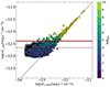 |
Fig. A.1. Comparison between Spitzer MIPS24 and WISE W4 photometry as a function of W4 S/N (see colour bar at right). The open circles in the background denote upper limits. W4 measurements systematically overestimate the actual fluxes at low S/N. The black solid (dotted) horizontal line marks the median (lowest 5 th percentile) flux for the objects in our sample without performing the quality cuts described in the text. The same holds for the red lines where the S/N≥2 cut is also applied. A significant amount of our sources would have systematically overestimated W4 fluxes. |
We also performed the same exercise to check the reliability of the W3 measurements. However, we only managed to perform this check on a much smaller (557 sources) sample of targets, obtained by cross-matching the Spitzer/IRAC and Spitzer/IRS data in the GOODS North and South fields (Giavalisco et al. 2004), as the wavelengths covered in this case are closer to the WISE W3. In order to evaluate the monochromatic flux at the W3 reference wavelength (12 μm), we logarithmically interpolated the flux of the two closest Spitzer bands, namely IRAC 8 μm and IRS 16 μm. We show the result of this match in Fig. A.2. Also in this case we observe a trail detaching from the one-to-one relation, although the average difference between the log Fν for Spitzer and WISE is lower than in the W4 vs. MIPS24 comparison (−0.22 dex after selecting sources with S/N W3 ≥ 2 against −0.42). Also in this case we observe the lowest S/N points being increasingly more offset from the identity line. In this case, however, even the lowest 5 th percentile of the flux distribution for the SDSS-WISE sample lies above the flux value where W3 starts to systematically overestimate the actual flux with respect to Spitzer. This implies that, within our sample, the effect of overestimating the W3 fluxes has a negligible impact.
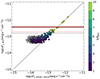 |
Fig. A.2. Comparison between the 12 μm fluxes interpolated between Spitzer IRAC 8 μm and IRS 16 μm and WISE W3, also showing the W3 S/N (see colour bar at right). The grey dots denote sources below the W3 S/N = 2 threshold chosen in this work. The black solid (dotted) horizontal line marks the median (lowest 5 th percentile) flux for the objects in our sample without performing the quality cuts described in the text. The same holds for the red lines where also the S/N≥2 cut is applied. Although there is a trail of points detaching from the one-to-one relation at low S/N W3 (∼4–5), roughly 95% of our sample has fluxes higher than the threshold where W3 starts to systematically overestimate the Spitzer measurements. The colour-code of the lines is the same as in Fig.A.1. |
Appendix B: The effect of redshift on the observed-frame band-pass filters
The appearance of the NIR bump at ≃3 μm in the broad-band photometric SED depends on its sampling in the observed-frame filters. As the redshift increases from z = 1.0 to z = 2.9, the NIR bump is sampled only in its rising part, thus leading to the loss of information about its real shape. Furthermore, the sampling in the observed frame also plays a role in the slight change of the position of the 1 μm dip. Here we show these effects at work on the Hernán-Caballero et al. (2016) spectral template, and how they affect the shape of the interpolated or extrapolated photometric SED.
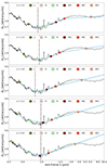 |
Fig. B.1. Effect of photometric sampling on the 1 μm dip and the NIR bump, here represented by the Hernán-Caballero et al. (2016) template (black), across the infrared filters (see legend) for increasing z. The light blue line represents the interpolated/extrapolated SED through the photometric points. The vertical dashed line marks the position of the minimum of the photometric SED. |
All Tables
Correlation parameters between z, log(Lbol), and alternative CF proxies also considering alternative datasets.
All Figures
|
Fig. 1. log(Lbol)–z plane for the sources surviving the binning selection and the colour cut (see text for details). The final sample spans roughly 2.5 decades in bolometric luminosity and covers up to z ∼ 2.9. The data are randomly coloured if the bin contains more than 30 objects to make the binning clearer. The black diamonds mark the average z and log(Lbol) values. The legend reports the fraction of sources having data in the labelled band. Since the sample is based on the cross-match between the SDSS and the AllWISE catalogues, all objects have data in the bands covered by these surveys, while only a minority have a full coverage across the several wave bands. |
| In the text | |
|
Fig. 2. Γ1–Γ2 plane for the sources satisfying the colour cut (magenta dots within the red circle). The light yellow square marks the average values reported in Richards et al. (2006) for blue unobscured quasars, while increasingly darker colours denote higher levels of reddening as labelled in the colour bar. |
| In the text | |
|
Fig. 3. Left: Pass-band integrated luminosity of the template with (empty diamonds) and without (filled diamonds) emission lines for a z = 1.0 quasar, according to the Vanden Berk (2001) template. Right: IGM transmission curves at different redshifts colour-coded as described in the legend. |
| In the text | |
|
Fig. 4. Example of average SEDs produced employing the uncorrected (left) and corrected (right) photometry (blue). The effect of the corrections applied is to increase the flux bluewards of the Lyα and reduce the optical and UV Fe II bumps. In addition, the strong Hα emission in the observed-frame H band (pink) is reduced in the corrected data-set. The grey clouds of points are the photometric data used to produce the SED; the coloured diamonds (same colour-code as in left panel of Fig. 3) are the median luminosities. The solid grey line represents the number of objects contributing to each spectral channel. The average quasar SED from Krawczyk et al. (2013), scaled to the 3000 Å total luminosity, is shown in green as a comparison. The light blue and orange shaded areas represent the regions where the Lopt and the LNIR terms in the covering factor proxy R are respectively evaluated (see Sect. 3.5). The average z and log(Lbol) of the parameter space represented by these SEDs are denoted in the top string. |
| In the text | |
|
Fig. 5. Left: Sequence of average SEDs for increasing luminosity, scaled by their total luminosity between 1000 Å and 1 μm. The trend of decreasing NIR luminosity for increasing optical luminosity is apparent despite the small dynamical range, and it is testified by the decreasing R shown in the inset. Here the mean value (standard deviation) is shown as a black solid (dashed) line. Right: Sequence of average SEDs for increasing redshift, scaled by their total luminosity between 1000 Å and 1 μm. The different sampling of the rest-frame emission leads to slightly different SEDs. However, on average R does not show any evolutionary trend as we do not observe systematic departures from the mean value. |
| In the text | |
|
Fig. 6. Composite SEDs from the simulated photometry of the template in the same redshift bins of the actual data. Here the magenta line marks the actual R value estimated using the total spectral template rather than the photometry. |
| In the text | |
|
Fig. 7. log(Lbol)–z plane with R shown as coloured dots (see colour bar at right). The black arrow points in the direction given by the PCA, evaluated in the bins within the black rectangle, while the dashed arrows show the uncertainty on the direction. The coloured rectangles highlight the bins of the parameter space shown in Fig. 8. We recall that the bins between 46.4 ≤ log(Lbol)≤47.4 and 1.0 ≤ z ≤ 2.8 are included in the SED evolution analysis described in Sect. 4.1. |
| In the text | |
|
Fig. 8. z–R (left panel) and log(Lbol)–R (right panel) section of the parameter space for the bins denoted by rectangles with the same colour-coding in Fig. 7. The solid lines represent the best linear fits to the data, while the shaded areas, obtained by resampling the posterior distributions of the best fit parameters, mark the 95% confidence intervals. |
| In the text | |
|
Fig. 9. Our full-sample SED and others from literature (see text). All the SEDs are normalised by their integrated luminosity between 1000 Å and 1 μm. The AGN spectral composite from Euclid Collaboration: Lusso et al. (2024) is scaled to match our SED (red solid line) at 2200 Å. The black line in the bottom panel shows the number of sources contributing per spectral channel in the average SED. The full-sample composite SED is available in its entirety in machine-readable form in the online journal. |
| In the text | |
|
Fig. 10. log(MBH)–log(Lbol) plane, with R shown as coloured dots (see colour bar at right). The black rectangle shows the region where the PCA was evaluated. The black solid and dotted arrows represent the direction of the strongest correlation as in Fig. 7. The dash-dotted line marks a constant λEdd = 0.2, representing the average value of the sample, while the magenta arrow shows the direction expected if the increase in R were driven uniquely by the decrease in λEdd. |
| In the text | |
|
Fig. 11. z–CF (left) and log(Lbol)–CF (right) section of the simulated parameter space. The CF and log(Lbol) values presented here are the observed (i.e. projected) quantities. The magenta diamonds represent the median CF values in bins of 0.2 dex in width. The y-axis uncertainties represent the standard error on the mean CF in the bin. The third axis is colour-coded. |
| In the text | |
|
Fig. 12. Obscured AGN fraction with NH > 1022 cm−2 as a function of redshift in different literature samples (Aird et al. 2015; Buchner et al. 2015; Ananna et al. 2019; Peca et al. 2023), including a correction for Compton-thick sources (see text for details). The data derived from the sources at log(Lbol)∼47 in our sample are shown as red dots. The S82 quasars in the same luminosity range exhibit similar values of R. The hollow rectangle shows the values covered by the CF derived according to the Stalevski et al. (2016) prescription. The average of the measured values and the inferred values are both extrapolated at the redshifts not directly covered by our bins at log(Lbol)∼47 as shown by the dashed lines. The black dotted and dash-dotted lines correspond to the Gilli et al. (2022) models for δ = 3.3, γ = 2.0, and, respectively, θ = 50° and 70°. |
| In the text | |
|
Fig. A.1. Comparison between Spitzer MIPS24 and WISE W4 photometry as a function of W4 S/N (see colour bar at right). The open circles in the background denote upper limits. W4 measurements systematically overestimate the actual fluxes at low S/N. The black solid (dotted) horizontal line marks the median (lowest 5 th percentile) flux for the objects in our sample without performing the quality cuts described in the text. The same holds for the red lines where the S/N≥2 cut is also applied. A significant amount of our sources would have systematically overestimated W4 fluxes. |
| In the text | |
|
Fig. A.2. Comparison between the 12 μm fluxes interpolated between Spitzer IRAC 8 μm and IRS 16 μm and WISE W3, also showing the W3 S/N (see colour bar at right). The grey dots denote sources below the W3 S/N = 2 threshold chosen in this work. The black solid (dotted) horizontal line marks the median (lowest 5 th percentile) flux for the objects in our sample without performing the quality cuts described in the text. The same holds for the red lines where also the S/N≥2 cut is applied. Although there is a trail of points detaching from the one-to-one relation at low S/N W3 (∼4–5), roughly 95% of our sample has fluxes higher than the threshold where W3 starts to systematically overestimate the Spitzer measurements. The colour-code of the lines is the same as in Fig.A.1. |
| In the text | |
|
Fig. B.1. Effect of photometric sampling on the 1 μm dip and the NIR bump, here represented by the Hernán-Caballero et al. (2016) template (black), across the infrared filters (see legend) for increasing z. The light blue line represents the interpolated/extrapolated SED through the photometric points. The vertical dashed line marks the position of the minimum of the photometric SED. |
| In the text | |
Current usage metrics show cumulative count of Article Views (full-text article views including HTML views, PDF and ePub downloads, according to the available data) and Abstracts Views on Vision4Press platform.
Data correspond to usage on the plateform after 2015. The current usage metrics is available 48-96 hours after online publication and is updated daily on week days.
Initial download of the metrics may take a while.