| Issue |
A&A
Volume 671, March 2023
|
|
|---|---|---|
| Article Number | A34 | |
| Number of page(s) | 19 | |
| Section | Extragalactic astronomy | |
| DOI | https://doi.org/10.1051/0004-6361/202244296 | |
| Published online | 02 March 2023 | |
The WISSH quasars project
XI. The mean spectral energy distribution and bolometric corrections of the most luminous quasars⋆
1
Dipartimento di Matematica e Fisica, Universitá Roma Tre, Via della Vasca Navale 84, 00146 Roma, Italy
e-mail: This email address is being protected from spambots. You need JavaScript enabled to view it.
2
INAF, Osservatorio Astronomico di Roma, Via Frascati 33, 00078 Monte Porzio Catone, Italy
3
INAF, Osservatorio Astronomico di Trieste, Via G. B. Tiepolo 11, 34143 Trieste, Italy
4
Dipartimento di Fisica, Sezione di Astronomia, Universitá di Trieste, Via Tiepolo 11, 34143 Trieste, Italy
5
INAF – Istituto di Astrofisica Spaziale e Fisica cosmica Milano, Via Alfonso Corti 12, 20133 Milano, Italy
6
INAF – Istituto di Astrofisica e Planetologia Spaziali, Via del Fosso del Cavaliere 100, 00133 Rome, Italy
7
INAF – Osservatorio Astrofisco di Arcetri, Largo E. Fermi 5, 50127 Firenze, Italy
8
INAF – Osservatorio Astronomico di Padova, Vicolo dell’Osservatorio 5, 35122 Padova, Italy
9
Dipartimento di Fisica e Astronomia, Universitá di Firenze, Via G. Sansone 1, 50019 Sesto Fiorentino (Firenze), Italy
10
ESO, Karl-Schwarschild-Strasse 2, 85748 Garching bei München, Germany
11
Kavli Institute for Cosmology, University of Cambridge, Cambridge CB3 0HE, UK
12
Cavendish Laboratory, University of Cambridge, Cambridge CB3 0HE, UK
13
Department of Physics and Astronomy, University College London, Gower Street, London WC1E 6BT, UK
14
Department of Physics, University of Rome ‘Tor Vergata’, Via della Ricerca Scientifica 1, 00133 Rome, Italy
15
Dipartimento di Fisica ‘G. Occhialini’, Università degli Studi di Milano-Bicocca, Piazza della Scienza 3, 20126 Milano, Italy
16
Dipartimento di Fisica e Astronomia “Augusto Righi”, Università degli Studi di Bologna, Via P. Gobetti 93/2, 40129 Bologna, Italy
17
INAF – Osservatorio di Astrofisica e Scienza dello Spazio, Via P. Gobetti 93/3, 40129 Bologna, Italy
Received:
17
June
2022
Accepted:
10
November
2022
Abstract
Context. Hyperluminous quasi-stellar objects (QSOs) are ideal laboratories to investigate active galactic nucleus (AGN) feedback mechanisms. Their formidable energy release causes powerful winds at all scales, and thus the maximum feedback is expected.
Aims. Our aim is to derive the mean spectral energy distribution (SED) of a sample of 85 WISE-SDSS selected hyperluminous (WISSH) quasars. Since the SED provides a direct way to investigate the AGN structure, our goal is to understand if quasars at the bright end of the luminosity function have peculiar properties compared to the bulk of the QSO population.
Methods. We collected all the available photometry, from X-rays to the far-infrared (FIR); each WISSH quasar is observed in at least 12 different bands. We then built a mean intrinsic SED after correcting for the dust extinction, absorption and emission lines, and intergalactic medium absorption. We also derived bolometric, IR band, and monochromatic luminosities together with bolometric corrections at λ = 5100 Å and 3 μm. We define a new relation for the 3 μm bolometric correction.
Results. We find that the mean SED of hyperluminous WISSH QSOs shows some differences compared to that of less luminous sources (i.e., a lower X-ray emission and a near- and mid-IR excess which can be explained assuming a larger dust contribution. WISSH QSOs have stronger emission from both warm (T ∼ 500 − 600 K) and very hot (T ≥ 1000 K) dust, the latter being responsible for shifting the typical dip of the AGN SED from 1.3 μm to 1.1 μm. We also derived the mean SEDs of two subsamples created based on their spectral features (presence of broad absorption lines and equivalent width of CIV line). We confirm that broad absorption lines (BALs) are X-ray weak and that they have a reddened UV-optical continuum. We also find that BALs tend to have stronger emission from the hot dust component. For sources with a weaker CIV line, our main result is the confirmation of their lower X-ray emission. By populating the LIR vs. z diagram proposed by Symeonidis & Page (MNRAS, 503, 3992), we found that ∼90% of WISSH QSOs with z ≥ 3.5 have their FIR emission dominated by star-forming activity.
Conclusions. This analysis suggests that hyperluminous QSOs have a peculiar SED compared to less luminous objects. It is therefore critical to use SED templates constructed exclusively from very bright quasar samples (such as this one) when dealing with particularly luminous sources, such as high-redshift QSOs.
Key words: galaxies: active / quasars: general
Full Tables 2–4 are only available at the CDS via anonymous ftp to cdsarc.cds.unistra.fr (130.79.128.5) or via https://cdsarc.cds.unistra.fr/viz-bin/cat/J/A+A/671/A34
© The Authors 2023
 Open Access article, published by EDP Sciences, under the terms of the Creative Commons Attribution License (https://creativecommons.org/licenses/by/4.0), which permits unrestricted use, distribution, and reproduction in any medium, provided the original work is properly cited.
This article is published in open access under the Subscribe to Open model. This email address is being protected from spambots. You need JavaScript enabled to view it. to support open access publication.
1. Introduction
The spectral energy distribution (SED) describes the emission of a source throughout the electromagnetic spectrum, and is therefore a powerful tool to investigate the physical processes originating it. In the case of active galactic nuclei (AGN), the study of their SED is particularly interesting since it extends to the whole electromagnetic spectrum, from the hard X-rays to the radio band.
The AGN SED is due to the sum of several contributions, arising from distinct regions and from different physical mechanisms. In particular, an actively accreting supermassive black hole (SMBH) is powered by the inflow of gas through an accretion disk with the subsequent transformation of gravitational energy into thermal energy, due to viscous torques (Lynden-Bell 1969). This process is responsible for the prominent blue bump in the UV and optical emission. The primary radiation can then be Compton up-scattered to X-ray energies in a region consisting of hot electron gas called the corona (e.g., Liang & Thompson 1979). Moreover, a dusty torus surrounding the accretion disk absorbs UV and optical photons and re-emits them in the near-IR (NIR) and mid-IR. In a similar way, dust at a lower temperature (T ≈ 20 − 100 K) located at much greater distances, heated by hot stars and partly by the central AGN, is responsible for the emission in the far-IR. Finally, the possible presence of a relativistic jet explains the radio emission in about 10% of the AGN (e.g., Blandford & Payne 1982). The study of SEDs is therefore primarily a direct way to investigate the AGN structure and a powerful tool to better understand the physical phenomena that are taking place.
Moreover, a precise determination of the SED allows us to compute the overall energy output of the AGN given by the bolometric luminosity Lbol (i.e., the integral under the SED). This is an important observational parameter in several studies and models of AGN feedback and AGN-host galaxy co-evolution (e.g., Ishibashi & Fabian 2012). Finally, the knowledge of the SED allows us to derive the bolometric correction (i.e., the ratio of Lbol to the luminosity in a given band), which is necessary to estimate the bolometric luminosity of sources for which multiwavelength observations are not available.
Elvis et al. (1994) first gave the composite SED of a sample of 47 type 1 quasars from the PG catalog extending from the X-rays to the radio band. In the following years SEDs from an increasing number of quasi-stellar objects (QSOs) were derived (e.g., Hatziminaoglou et al. 2005; Shang et al. 2011; Bianchini et al. 2019). Notably, Richards et al. (2006) computed the mean SED from a sample of 259 quasars with both SDSS and Spitzer IRAC photometry. Krawczyk et al. (2013; hereafter K13) extended their work using a sample of 108 184 non-reddened type 1 quasars at 0.064 < z < 5.46 with at least SDSS photometry to construct a mean SED between 10 keV and ∼20.0 μm, which is the most robust according to the number of sources used.
Both Richards et al. (2006) and K13 constructed the composite SEDs of some subsamples based on the luminosity of the QSOs; the SEDs obtained in these works are similar to the value originally derived by Elvis et al. (1994), although with small differences, and their study reveals that the shape of AGN emission is generally comparable over a wide range of luminosities. Hao et al. (2014), using 407 quasars from COSMOS investigated the dependence of the SED shape on several physical properties of the sources (redshift, Lbol, MBH, Eddington ratio) and no significant correlation was found.
However, the fact that bolometric corrections seem to be luminosity dependent (e.g., Runnoe et al. 2012a; Duras et al. 2020) and that the ratio of X-ray to optical luminosity (i.e., αOX) decreases for optically bright QSOs (e.g., Steffen et al. 2006) necessarily implies some kind of evolution in the shape of the SED. While SEDs derived from large statistical samples are robust and exceptionally effective in representing the average properties, they might fail in the description of distinctive features specific to a particular subclass of AGN. For this reason, when analyzing sources with some peculiar properties, it might not be appropriate to rely on SEDs built from extremely varied samples, but rather it is preferable to use those that have been derived from QSOs with similar features.
A population of AGN particularly interesting to study is represented by quasars at the bright end of the luminosity function since theory and observations both suggest that these are the sources where feedback is strongest (e.g., Veilleux et al. 2013; Cicone et al. 2014; Fiore et al. 2017; Bischetti et al. 2019; Fluetsch et al. 2019; Lutz et al. 2020). In the catalog used by K13 there are several QSOs with Lbol up to 1048 erg s−1, although they represent only a small fraction, even considering their subsample of optically bright sources (∼2.8% of the whole sample has Lbol ≥ 1047 erg s−1). Therefore, the resulting composite SED is not really representative of these few hyperluminous sources, but of the bulk of the population at lower luminosities.
In this paper we compute the composite SED of WISSH quasars, a sample consisting of 85 type 1 QSOs selected to be among the most luminous in the Universe. Throughout the paper we assume a flat ΛCDM cosmology with H0 = 70 km s−1 Mpc−1 and ΩΛ = 0.70.
2. The WISSH sample
The WISSH sample (Bischetti et al. 2017) is composed of 85 type 1 radio-quiet hyperluminous quasars with log(Lbol/[erg s−1]) ≥ 47.0 (Duras et al. 2017). The sample was assembled cross-correlating the SDSS (Shen et al. 2011) and the WISE (Wright et al. 2010) catalogs and selecting, among the sources with a flux density Sv, 22 μm > 3 mJy, the 100 most luminous QSOs at λ = 7.8 μm (Weedman et al. 2012). Gravitationally lensed objects, those that had a contaminated WISE photometry, and those with an anomalous radio emission were then removed, leaving the final sample of 85 quasars with 46.96 ≤ L7.8 μm/[erg s−1] ≤ 47.49 and a redshift distribution 1.8 < z < 4.7.
Given their high luminosities and their redshift distribution covering the epoch where both AGN activity and star formation were at their peak (e.g., Ueda et al. 2003; Hasinger et al. 2005; Madau & Dickinson 2014), WISSH quasars are the ideal targets to investigate the feedback mechanism. Several previous works on the sample have indeed shown the exceptional nature of these sources in their ability to drive powerful winds at different scales.
For example, Bruni et al. (2019) analyzed the broad absorption line (BAL) population in WISSH and found that it represents a larger fraction when compared to other samples (24% of sources with CIV balnicity index > 0 compared to 13.5% found by Gibson et al. 2009), confirming that high Lbol favors the acceleration of nuclear-scale winds. Moreover, using the [OIII] and CIV emission lines as tracers of ionized gas, the velocity and the kinetic power of the outflows were measured for different sources on scales up to 7−10 kpc, finding mass outflow rates among the highest reported in the literature (Bischetti et al. 2017; Vietri et al. 2018). From the analysis of Lyman-α emitting nebulae surrounding one QSO, Travascio et al. (2020) also found evidence for outflowing gas at circumgalactic scale. Finally, it has been found that these quasars are located in extremely overdense environments (see Bischetti et al. 2018, 2021).
In Table 1 WISSH quasars are listed along with their coordinates, their redshifts, and their identification number. Redshifts, when available, are taken from Bischetti et al. (2017, 2021), Vietri et al. (2018), and Yi et al. (2020) and from the SUPER survey (Kakkad et al. 2020; Vietri et al. 2020); otherwise, we use values provided by Hewett & Wild (2010) who derived redshifts without including the CIV emission line in the computation. As shown by Vietri et al. (2018), the CIV line can lead to a systemic underestimation of the redshift. This leaves us with 12 QSOs without an assigned redshift; for these sources we adopt the value provided by the most recent SDSS Quasar Catalog Data Release (Lyke et al. 2020; Pâris et al. 2014).
WISSH sample: ID, coordinates and redshift.
3. Multiwavelength photometry
By construction of the sample, all 85 WISSH QSOs have SDSS photometry in the ugriz filters and were detected in each of the four WISE bands at λ = 3.3, 4.6, 12, and 22 μm. In addition, 2MASS photometry in the J, H, and K bands was collected for roughly 80% of the sample, while the remaining QSOs were targets of an observational campaign conducted by our group with TNG-NICS (see Appendix A). Therefore, for all sources we have photometry in 12 observed bands between λ = 3500 Å and λ = 22 μm.
Moreover, in the far-IR, Duras et al. (2017) used Herschel archival data to recover the flux density of 16 QSOs for the three SPIRE bands at λ = 250, 350, and 500 μm. The far-IR coverage is also provided by the observations of nine QSOs (five of which are among those with Herschel data) performed with ALMA, NOEMA, and JVLA in the ∼30 − 350 GHz frequency range (Bischetti et al. 2021).
Given the poor Herschel angular resolution (18.1″, 25.2″, and 36.6″ beams FWHM, at λ = 250, 350 and 500 μm respectively, versus ∼1.0 × 0.8 arcsec2 and ∼3.5 × 2.1 arcsec2 of ALMA and NOEMA, respectively), the measured flux could be contaminated by the emission of nearby sources. Bussmann et al. (2015), Trakhtenbrot et al. (2017) and Hatziminaoglou et al. (2018) estimated the multiplicity rate to be between 30% and 50%. In the WISSH sample, ALMA and NOEMA observations revealed the presence of at least one nearby companion galaxy, (i.e., in the same field of view as the telescope, which has a diameter of about 20−30″ for both ALMA and NOEMA, Bischetti et al. 2018) in seven out of nine QSOs, although only in two cases have their fluxes been constrained and are found to represent 50% and 27% of the total observed emission. For the other QSOs, only 3σ upper limits on the contributions of their neighboring companions could be determined, and range between 0.2% and 54% (Bischetti et al. 2021). For the five QSOs with both Herschel and ALMA/NOEMA data, we subtracted companion fluxes in the 250, 350, and 500 μm bands assuming that they made the same contribution as observed with ALMA/NOEMA; for those sources with unconstrained fluxes, we removed half of their upper limits. For the remaining Herschel-observed sources we did not apply any corrections; however, based on what we found for the other QSOs, we estimate that on average their fluxes may be overestimated by roughly ∼25%. Finally, in the X-ray region, the 2 − 10 keV integrated fluxes of 43 sources are available thanks to Chandra or XMM-Newton detections (Martocchia et al. 2017; Zappacosta et al. 2020).
Although WISSH photometry has been collected over an extended period of time and the same QSOs might have been observed in different bands a long time apart, we do not expect our data to be drastically affected by source variability. It has been shown (e.g., Vanden Berk et al. 2004; Caplar et al. 2017) that AGN variability clearly anti-correlates with luminosity, and therefore it should not constitute a real issue for WISSH hyperluminous sources. A table with the entire photometry of the WISSH sample is reported at the CDS. The description of the columns is given in Table 2. Magnitudes are AB and have been corrected for the galactic extinction (Schlafly & Finkbeiner 2011).
Reference table for the WISSH sample photometry.
4. Construction of the mean SED
4.1. Removing photometric data significantly affected by extinction
The analyzed sample is composed of type 1 unobcured QSOs. Nevertheless, a fraction of them shows a redder spectrum compared to classical unobscured quasars, which can be explained in terms of dust reddening of the (bluer) intrinsic spectrum.
To select obscured quasars we computed the optical spectral slope αopt between λ = 0.3 μm and λ = 1 μm. We identified as obscured those with αopt < 0.2, corresponding to an EB − V ≥ 0.15 assuming the mean SED from Richards et al. (2006; see Fig. 5 in Bongiorno et al. 2012). A total of seven QSOs (WISSH25, WISSH34, WISSH49, WISSH55, WISSH58, WISSH73, and WISSH74) were found to satisfy this criterion. These QSOs also satisfy the criterion proposed by Glikman et al. (2004) for identifying red quasars (i.e., r − K > 4 and J − K > 1.7), while only WISSH74 would also be classified as an extremely red QSOs according to the criterion by Ross et al. (2015; i.e., r − W4 ≳ 7.5). Moreover, Glikman et al. (2022) define as red QSOs sources with EB − V > 0.25. According to this definition only WISSH34, WISSH49, and WISSH74 are properly red (see Table 3); for the other four sources it would perhaps be more appropriate to use the term reddish. Since the blue part of the SED of these objects does not reflect their intrinsic emission, we excluded their photometry at wavelengths shorter than 1.0 μm in the computation of the mean SED.
Bolometric and monochromatic luminosities for WISSH quasars.
Moreover, since the work from Bruni et al. (2019) outlined the presence of BAL in a significant fraction of the objects, we visually inspected the SDSS spectra and removed the photometry that was clearly depressed due to the presence of BAL features. After corrections were applied (see Sect. 4.2), we replaced these points with non-absorbed data, using the mean SED by K13 normalized to the nearest filter available (Gap repair). This procedure was applied for a total of 11 QSOs, mostly for the u and g bands. Their repaired photometry is shown as gray circles in Fig. 3.
4.2. Corrections
There are several factors that modify the observed radiation with respect to the intrinsic emission of an AGN. Since we are interested in reconstructing the mean intrinsic SED of hyperluminous QSOs, it is necessary to determine the contributions provided by these factors and correct the data for them. In particular, following the same procedure also adopted by K13 we considered the absorption of the intergalactic medium, the contamination of the spectral emission lines from broad- and narrow-line regions and the contribution from the host galaxy. The methods we employed to determine the corrections to be applied are indirect and are based on statistical grounds. To this extent, the correcting factors they provide for a single QSO are not necessarily true; however, when averaged over the whole sample, they should give a fairly accurate result. For this reason we used corrected photometry only in the derivation of the mean SED(s); when dealing with the computation of individual QSO properties (e.g., Sect. 5.4.1), we do not apply any corrections.
4.2.1. (i) Intergalactic medium absorption
One of the main problems that arise when reconstructing the SED of a distant source is the absorption due to the intergalactic medium (IGM) mainly constituted of neutral hydrogen clouds distributed along the line of sight and responsible for the drastic drop in the observed flux blueward the Lyα line at λ = 1216 Å. One way to account for this effect is to assume a statistical distribution of the absorbers and evaluate the expected transmission function Tλ = e−τ(z, λ), where τ is the optical depth.
We used the results from Inoue et al. (2014), who developed an analytical model to estimate the optical depth τ as a function of the source’s redshift. In the model from Inoue et al. (2014) the evolution of the number density distribution of the HI clouds is described separately for two components, the Lyα forest component and the damped Lyα systems, the former being dominant for a column density log(NHI/cm−2) < 17.2 and the latter for log(NHI/cm−2)≥20.3 and with a mixed contribution for intermediate values. To be conservative in our corrections, we assumed no damped Lyα component when evaluating the optical depth. Once the optical depth has been derived, it can be transformed in magnitude correction for the five SDSS filters by convolving the IGM attenuation with the filter transmission Sλ and the continuum flux Fλ
where the UV-to-optical continuum flux for each QSO was modeled as a single power law Fλ ∝ λ−1.56 (Vanden Berk et al. 2001). Non-extincted magnitudes are then recovered as

For the analyzed sample we find that ΔmIGM ranges between 0.02 and 3.96 (1.21 on average) for the u filter and between 0 and 2.65 (0.48 on average) for the g filter.
4.2.2. (ii) Emission lines
AGN are characterized by several emission lines in their spectra. If these lines fall into an observed filter, they lead to an overestimation of the source flux. In order to remove this effect we built a mock template of the continuum flux f(c) and we added the 13 strongest emission lines measured by Vanden Berk et al. (2001) in their composite spectrum, f(c & l). As in Sect. 4.2 (i) the continuum flux was modeled as a single power law, while the emission lines were modeled as Gaussian functions using the equivalent widths and the FWHMs provided by Vanden Berk et al. (2001; see Fig. 1). A possible issue related to this procedure is that we neglected the well-known luminosity dependence of the lines equivalent width (e.g., Baldwin et al. 1989; Pogge & Peterson 1992; Bian et al. 2012). Moreover, in this approximation, for simplicity reasons, the skewness of the line profiles was neglected. We also neglected the equivalent width dependence.
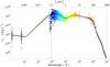 |
Fig. 3. Mean SED derived from the WISSH sample. The shaded area gives the 68% confidence interval. The colored circles represent available data points, color-coded according to the filter in which they were observed. Photometry obtained by Gap Repair is represented as gray circles. The gray crosses indicate X-ray luminosities reconstructed from the αOX relationship. The dotted black line indicates the Lyman limit λL = 912 Å: for shorter wavelengths the mean SED was truncated and extended as explained in Sect. 4.4. |
The f(c & l) template is shifted for each source, depending on its redshift. The correction is
Therefore, the corrected magnitudes are given by

The correction was performed over the five SDSS filters; the J, H, and K filters from 2MASS or TNG and for W1 and W2 in which emission lines fall given the redshift range of each WISSH QSO. Figure 1 shows the observed and corrected fluxes (both for IGM and emission lines) for a source at z = 4.40 as an example.
4.2.3. (iii) Host galaxy contamination
Another contribution that should be removed before computing the intrinsic AGN SED is provided by the host galaxy. In the absence of observations allowing for a direct measurement of the light coming from the host, we must infer Lhost from total observed radiation Ltot = LAGN + Lhost. Shen et al. (2011) provided a relationship between LAGN and Lhost which is suitable for the case of luminous QSOs

where x + 44 ≡ log(L5100, tot/[erg s−1]). This formula is valid for log(L5100, tot) < 45.053. At higher luminosities the host contribution is assumed to be negligible.
For the WISSH sample we extrapolated L5100 by linearly interpolating the data from the two nearest bandpasses. All 85 sources have log(L5100) > 45.053 (see Fig. 3 and Table 3), so no corrections for the host were applied.
4.3. Interpolation and construction of the mean SED
We linearly interpolated (in the log–log space) the individual SEDs in order to have them binned equally. In detail, we interpolated the luminosity points over a grid of width Δ(log λ) = 0.02. The errors on the interpolated points were computed linking the upper (or lower) bounds of the adjacent observed luminosities. The mean SED for each wavelength of the grid  was subsequently derived as the weighted geometric mean of the points
where wi ≡ (λLi/σi)2 are the weights, and λLi and σi are the interpolated luminosities and their associated errors, respectively.
Errors on the average SED are evaluated as the geometric variance
and the confidence interval is given as
Since 4 of the 16 sources with available Herschel photometry have at least one band where they are undetected (usually the 500 μm band, where only the upper limits on their fluxes are available), we performed gap repair using our own SED; in detail, we first built a mean SED using only the remaining 12 QSOs with complete Herschel detections and used this one to replace the upper limits with a fixed luminosity value. The gap repair SED was also used for the four QSOs with available far-IR (FIR) ALMA or NOEMA data but lacking Herschel observations, and to reconstruct the FIR emission of the three sources undetected by NOEMA and for which we only have upper limits. Finally, we derived rest-frame 10 μm repaired photometry for all 85 QSOs with the aim of avoiding abrupt changes in the mean SED shape, where the gradually decreasing number of sources is due to their different redshift distributions. It should be noted that this last photometry repair is only intended to provide a smooth SED template in the range 9 μm ≲λ ≲ 50 μm where, in the absence of observational data, we are forced to reconstruct the shape of the SED. For this wavelength interval, our mean SED cannot be considered representative of the true emission by highly luminous QSOs. This also explains why the prominent ∼10 μm silicate feature commonly observed in QSO spectra (e.g., Siebenmorgen et al. 2005) is not visible in our mean SED.
4.4. X-ray and extreme ultraviolet range
To characterize the mean SED in the X-ray region we employed photon indexes Γ recovered in the work by Martocchia et al. (2017) and Zappacosta et al. (2020) to transform the absorption corrected integrated luminosities into 2 and 10 keV monochromatic luminosities, assuming a power-law trend Lν ∝ ν1 − Γ. For sources for which we do not have X-ray data, we used the known relationship between L2500 Å and the αOX (Vignali et al. 2003; Steffen et al. 2006; Lusso et al. 2010) to estimate the 2 keV luminosity. In detail, we employed the relationship provided by Martocchia et al. (2017), which is in excellent agreement with the others in the literature, and was derived using the WISSH sample; we derived L2500 Å by linearly interpolating two adjacent luminosity points. For these sources we then estimated the 10 keV luminosity assuming a standard value Γ = 1.8 (Piconcelli et al. 2005; Martocchia et al. 2017). Given the wide spread of the observed X-ray luminosities, including these reconstructed values does not affect the mean SED (see Fig. 2 and also Fig. 3 where reconstructed X-ray luminosities are plotted as gray crosses).
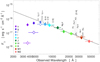 |
Fig. 1. Example of corrections applied to take into account both IGM absorption and emission lines for WISSH23 at z = 4.4. The empty diamonds represent the observed fluxes, while the filled diamonds are the fluxes after corrections. The horizontal bars indicate the range of wavelengths covered by the filters. |
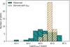 |
Fig. 2. 2 keV luminosity distribution of the sample. We include both measured values (green histogram) by Martocchia et al. (2017) and Zappacosta et al. (2020) and derived values using the L2 keV − L2500 Å relation. |
Between the X-ray band and the bluer UV filter, there is a rather wide unsampled region of the spectrum; in fact, for 100 Å ≲λ ≲ 1200 Å, and especially below the Lyman limit (λL = 912 Å), the absorption by hydrogen clouds is responsible for the almost total absorption of the emitted photons. These wavelengths are around the peak of AGN emission (the so-called blue bump from the accretion disk). Since computing the bolometric luminosities of the QSOs is among the goals of this work, and Lbol is given by the integral of the SED, it is necessary to find a way to extrapolate the shape of the SED in this extreme ultraviolet (EUV) region.
In the literature there are several works dedicated to the characterization of the AGN SED in the EUV (Mathews & Ferland 1987; Korista et al. 1997; Scott et al. 2004; Casebeer et al. 2006; Stevans et al. 2014; Lusso et al. 2015); we opted to use the broken power law discussed by Lusso et al. (2010) as it uses observations by Zheng et al. (1997) to define the QSO average spectrum up to λ = 500 Å, which, despite not being among the most recent ones, provides a more conservative estimate of the flux (i.e., it has a steeper slope). In detail, we truncated the mean SED at the Lyman limit and proceeded to extend it with a fixed slope power law with αλ = 0.8 up to λ = 500 Å; we then linearly connected the end of this curve with that of the 1−10 keV power law. Thus, the X-ray to UV region of the mean SED takes the form
The characterization of the EUV band directly affects the measured value of Lbol. Since several other authors (including K13 and Runnoe et al. 2012a, with whom we compare) prefer to use a single power law to link the UV to the X-rays, we quantified the impact of using a double power law rather than a single spectral slope, finding that in our case the double PL option leads to a 5% higher Lbol measurement.
The resulting full mean SED from the WISSH sample, extending from 10 keV to ∼1000 μm, is shown in Fig. 3 and given in Table 4. We indicate with a dashed line those parts of the mean SED that were reconstructed.
Mean SEDs computed for the WISSH full sample and for the subsamples: BAL, non-BAL, REWCIV < 25 Å, REWCIV ≥ 25 Å.
5. Results
5.1. Comparison with previously derived AGN mean SED
In this section we compare the shape of the derived mean SED with that reported in the literature. Given the extreme luminosities of the WISSH sample compared to the bulk of the population, to ease the comparison it is necessary to normalize the SEDs at a given wavelength. In this respect, the comparison has to be intended as relative differences, obtained assuming an equal luminosity at the normalization wavelength.
In Fig. 4 we show the comparison of the WISSH SED with the overall mean SED by K13; in addition to being one of the statistically most robust composite SEDs in the literature, it was derived following a procedure very similar to the one adopted here. Therefore, the SED by K13 is particularly suitable for making a comparison between the typical emission of type 1 QSOs and that by our hyperluminous sources. We also include in the plot the mean SED derived by K13 for their high-luminosity subsample (log(λL2500 Å/[erg s−1]) ≥ 45.85, corresponding to 46 ≲ log(Lbol/[erg s−1]) ≲ 47.5). All SEDs are normalized at λ = 1.3 μm which corresponds approximately to the dip between the accretion disk UV bump and the obscuring torus mid-IR emission. To make a comparison that is independent of the wavelength chosen for normalization, in our analysis, where possible, the comparison was made either in terms of spectral slopes (i.e., luminosity ratios) or in terms of the percentage of emission of one component relative to another.
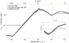 |
Fig. 4. Comparison between the WISSH mean SED derived in this work (black line), the overall mean SED for type 1 QSOs by K13 (light blue line), and the high-luminosity SED also by K13 (dotted red line). SEDs are normalized at 1.3 μm (dotted vertical line). The inset shows an image of the SEDs zoomed-in on the 0.7 < λ/μm < 6 range. |
Overall, SEDs are quite similar in shape and, as expected, differences are marginally less pronounced when the comparison is made with respect to the high-luminosity mean SED by K13. There are, however, some significant discrepancies, in particular in the X-ray and in the NIR and mid-IR bands.
5.2. X-ray to optical bands
At high energies, we find that the SED of hyperluminous quasars has a lower X-ray emission compared to that of the bulk of the AGN population. This is due to the nonlinear relationship between the UV and X-ray luminosity, expressed through the αOX, and more precisely to the well-known anti-correlation between αOX and L2500 Å (see references in Sect. 4.1) meaning that UV luminous QSOs are relatively X-ray weak. We find αOX = −1.94 for the WISSH mean SED (αOX = −1.91 considering only sources with X-ray observed data), while for comparison the K13 mean SED has αOX = −1.53. It should be noted that these values, being  , do not depend on the parameterization chosen to reconstruct the EUV SED.
Smaller differences (within the 3σ confidence interval, assuming the same L1.3 μm) between the WISSH mean SED and the K13 one have also been found in the UV region, between the Lyα and Lyman limit, where we observe a decline in the emission of hyperluminous quasars that is not present in either of the two SEDs provided by K13. This can likely be attributed to our conservative estimates made in terms of IGM absorption (i.e., not considering Damped Lyα systems which could instead be relevant especially for our high-z QSOs) and to a redshift effect on the edge. In addition, in the optical band, approximately between λ = 3000 Å and 8000 Å, we note that the WISSH mean SED and the K13 high-luminosity SED both have a steeper continuum. The WISSH mean SED and K13 high-luminosity subsample have αopt = 0.8 ± 0.1 and 0.85, respectively, to be compared with αopt = 0.65 exhibited by the whole K13 sample. This difference could be the result of a primary UV component having higher temperatures, as could be expected in this class of highly luminous AGN.
5.3. IR region
In the NIR and mid-IR, for λ > 1 μm, the WISSH mean SED shows a more prominent bump at 3−9 μm with a ∼5σ significance at 5 μm (again, assuming the same L1.3 μm), and a dip shifted to slightly shorter wavelengths (i.e., λdip ≈ 1.1 μm), while in both SEDs by K13 (and also those by Elvis et al. 1994; Richards et al. 2006) it is found at λ ≈ 1.3 μm. Although providing a statistical significance to this shift in wavelength is not easy, we are confident that it is not an artifact nor does it depend on the method adopted, since it is four times the resolution of the grid adopted to interpolate the data points and the procedures adopted by Richards et al. (2006) or K13 to derive their mean SEDs are fairly analogous to ours. However, there are at least two factors that we cannot rule out that may have influenced our result. First, the limited number of WISSH QSOs may not be sufficient to adequately sample a region where a sudden change in slope occurs. Second, our results could be influenced, at least partially, by host emission that peaks around those wavelengths, and which we assumed is negligible (see Sect. 4.2). The change in the dip position will be the focus of a future work (Saccheo et al., in prep.).
We quantified the WISSH NIR to mid-IR excess by using the ratio of the integrated IR to optical emission: R ≡ L1.3 − 9 μm/L1216 Å−1.3 μm. We found that, for WISSH QSOs, R is ≈32% higher than that obtained from the K13 high-luminosity SED. Alternatively, by normalizing the IR emission to the luminosity at the dip between the disk and torus bumps (i.e., L1.3 − 9 μm/Ldip) we get a ∼29% excess, which is consistent with the previous result. The stronger bump is not unexpected since the sources of the sample were specifically selected to be the most luminous at λ = 7.8 μm. Moreover both works by Richards et al. (2006) and K13 show that luminous quasars tend to have a stronger IR emission. In addition, Duras et al. (2017), analyzing a subsample of 16 WISSH quasars, had already pointed out that in about 30% of the sources an additional emission component was needed to properly model the NIR to mid-IR emission; they accounted for this IR excess with an extra hot dust component whose temperature ranges from 650 to 850 K depending on the source. However, in none of these works was a shift of the dip reported.
To further verify the hypothesis of an extra hot dust component, we tried to reproduce the WISSH SED curve at 0.8 < λ/μm < 8 by fitting a combination of the mean SED by K13 plus a modified blackbody with temperature free to vary in the range 150−1600 K as

where a and b are the relative normalizations. The best fit, according to χ2 minimization, is obtained with the addition of a BB at T = 520 K and is shown as the solid orange line in the top panel of Fig. 5. As can be seen, this extra dust component optimally describes the mid-IR bump, but fails to explain the shift of the dip since the emission of a blackbody with such a temperature is negligible at these wavelengths, and a hotter component is therefore required. As the next step, we shape the mean SED by including two blackbodies with two distinct ranges of possible temperatures, Thot ∼ 900 − 1600 K and Twarm ∼ 150 − 900 K (Hernán-Caballero et al. 2016):

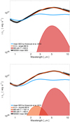 |
Fig. 5. Modeling of the WISSH mean SED via the K13 composite SED plus one (top panel) or two (bottom panel) modified blackbodies, as described in Sect. 5.1. A comparison of the two solid orange lines shows how the addition of a hotter dust component allows a better reproduction of the curve for λ < 2 μm. |
The best-fit solution, shown in the lower panel of Fig. 5, includes a BB at Thot = 1021 K and one at Twarm = 460 K1. Both the NIR excess and the shift of the dip are now reproduced. The WISSH sources therefore have an IR excess with respect to the mean QSO SED, which is due to two distinct contributions: (1) a higher emission by a warm dust component (T ∼ 450 − 800 K) heated by the AGN and likely associated with the obscuring torus, which is explainable as a larger covering factor of the torus itself; (2) extra emission by very hot dust (T > 1000 K), which is responsible for the NIR excess and the shift of the dip.
In the attempt to provide a physical explanation and account for these extra hot and warm dust components, we used SKIRTOR by Stalevski et al. (2012; in the version implemented in CIGALE, Yang et al. 2022) to generate several AGN SED templates and fit the mean SED between λ = 1216 Å and λ = 8 μm. In detail, we narrowed the parameter space by fixing the viewing angle to 0, since the strong NIR emission suggests that the inner layer of the torus is directly visible (see also Duras et al. 2017).
The best-fit results are reported in Fig. 6 and show that although there is very good agreement at λ ≳ 1.5 μm, this is not true for wavelengths around the minimum where no model seems to be able to describe the shape of our SED. We also considered a polar dust component since in some cases it was found to be necessary to explain the strong NIR emission of HDO AGN (e.g., Lyu & Rieke 2018). However, a large contribution from this component would be associated with a strong extinction of the optical continuum that we do not observe in our QSOs; indeed, in our fit the polar dust gives a completely negligible contribution, and thus cannot represent the extra hot dust component discussed above. Therefore, while the extra emission that we attributed to an additional warm dust component in our empirically driven reasoning can be justified as a specific configuration of the torus geometry, we are unable to explain the nature of the hot component.
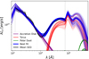 |
Fig. 6. Best-fit and 1σ errors of the WISSH mean SED via CIGALE-generated templates. For illustrative purposes the different components considered in CIGALE and whose sum provides the overall AGN SED are plotted in different colors. The best-fit parameters are OA = 50°, τν = 11, p = 1.0, q = 0, δAD = −0.4, Rin/Rout = 20, TPD = 100 K, EB − V = 0.03 (see Yang et al. 2022, for a detailed description of these parameters). The dotted lines delimit the wavelength range over which the fitting was performed. |
5.4. Bolometric luminosities and bolometric corrections
5.4.1. Bolometric luminosities
The bolometric luminosity is defined as the integrated area below the non-extincted SED. It provides a measure of the energy budget of the AGN at all wavelengths (see below for details).
Fluxes, which are the actual measured physical quantity, are converted into luminosities under the hypothesis that the sources emit isotropically:
Under the isotropic assumption, when computing Lbol, it is necessary to consider only the radiation emitted along the line of sight and remove from the calculation the reprocessed radiation (i.e., that of the obscuring torus), which is heated by photons originally emitted in another direction and whose contribution is already included in the 4π factor in the above equation. To avoid counting the same contribution twice, several authors (e.g., Marconi et al. 2004; Nemmen & Brotherton 2010; Lusso et al. 2012; Runnoe et al. 2012a; Duras et al. 2020) limit the integral under the SED to λ < 1 μm. Regarding the high-energy integration limit, several authors (e.g., K13, Duras et al. 2020) use similar reasoning to that seen for the IR and place it in the soft X-ray band (between 0.5 and 2 keV) to avoid counting radiation reprocessed by the corona and consider only the proper accretion luminosity. However, in our case, to be consistent with Runnoe et al. (2012a), we decided to set the limit at 10 keV.
To derive Lbol we model each source emission data point with the derived mean SED plus a dust extinction component (see, e.g., Bongiorno et al. 2012)

where the extinction A(λ) is computed assuming the SMC dust reddening law by Prevot et al. (1984; i.e., A(λ) = 1.39λ−1.2EB − V, λ in μm). By χ2 minimization procedure with respect to the observed luminosity points in the range 1216 Å ≤ λ ≤ 10 μm we obtain the best values for the normalization a and the color excess EB − V. We set the lower limit to 1216 Å because for shorter wavelengths the drop in the observed flux is not completely attributable to dust extinction but also to IGM absorption. The value of Lbol is then derived by integrating the normalized non-extincted mean SED between 1 μm and 10 keV.
To calculate the associated errors first, if needed, we gradually increased the uncertainties on the luminosity points until we met the condition  (e.g., Gruppioni et al. 2008, but see also Andrae 2010 for a discussion about the underlying assumptions and the shortcomings of this procedure). Then we found the lower and the upper errors as the minimum and maximum values among the models that satisfy the condition
  ; to these uncertainties we added in quadrature those related to the Lbol of the mean SED, calculated as the difference obtained if we integrate the lower (or upper) bounds instead of its average value. We also considered an additional contribution to the overall uncertainties, given by the difference between Lbol computed using the mean SED and that derived by connecting their intrinsic luminosity point with straight lines. This component is particularly relevant for QSOs with EB − V = 0 and that have an intrinsic bluer SED than the average one; this way we take into account that their Lbol might be underestimated.
The derived Lbol are reported along with intrinsic monochromatic luminosities at different wavelengths and the EB − V in Table 3, and their distributions are shown in Fig. 7.
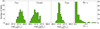 |
Fig. 7. Bolometric and monochromatic luminosities distributions of the WISSH sample. From left to right: Bolometric luminosities, intrinsic monochromatic luminosities at 5100 Å and 3 μm, and EB − V. |
5.4.2. Bolometric corrections
We then used the derived Lbol to compute the bolometric correction (i.e., the ratio of the bolometric luminosity to the monochromatic luminosity in a specific band):  . In particular, we derived bolometric corrections for λ = 5100 Å and 3 μm, two bands where the WISSH mean SED shows differences with respect to the K13 SED. The purpose of our analysis is twofold. On the one hand, we are interested in inspecting how WISSH QSOs compare with the bulk of the population and with other sources with comparable luminosity; on the other hand, we have the opportunity to study bolometric corrections in an as-yet poorly explored luminosity range. It is widely accepted (e.g., Lusso et al. 2012; Runnoe et al. 2012a; Duras et al. 2020) that in most bands bolometric corrections are not constant, but instead are functions of Lbol. WISSH quasars are therefore excellent sources to investigate these dependences at the bright end of the AGN luminosity distribution. Notably, Duras et al. (2020) already included WISSH QSOs in their study of X-ray (2−10 keV) and 4400 Å bolometric corrections across seven orders of magnitude of quasar luminosity.
In Fig. 8 we show K5100 Å (upper panel) and K3 μm (lower panel) versus Lbol; we have also included QSOs by Runnoe et al. (2012a) and K13. To give a clearer visualization of the position in the plot of the majority of QSOs by K13 we depict as black circles the median values obtained by grouping the sources in bins spaced 0.15 dex in Lbol. It should be noted that by inserting all these sources in the same plot we are assuming that any dependence on redshift is negligible.
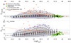 |
Fig. 8. Bolometric corrections at λ = 5100 Å and 3 μm vs. Lbol. Top panel: K5100 Å vs. Log(Lbol), in units of [erg s−1]. QSOs from Runnoe et al. (2012a) are shown as orange filled circles. Gray circles depict QSOs from Krawczyk et al. (2013), while black circles provide their median values (with the associated spread) over bins of width 0.15 dex. WISSH QSOs are shown as green squares, and the black square indicates their mean. The solid orange line describe the nonlinear relationship by Runnoe et al. (2012a), the dotted line indicates that the relation is being extrapolated to lower or higher luminosities. The dashed black lines give the linear relationship by K13 and its associated uncertainty. Bottom panel: K3 μm vs. Log(Lbol), color-coded as above. Here the dashed black lines depict the best fit computed as explained in Sect. 5.4.1 and its uncertainty computed as the square root of the variance with respect to the best-fit prediction. |
In detail, Runnoe et al. (2012a) derived bolometric corrections for a variety of wavelengths using 63 sources with 45 ≲ log(Lbol/[erg s−1]) ≲ 47 at 0.3 ≤ z ≤ 1.4. They found that nonlinear relationships in the form of log(Lbol) = Alog(Lλ)+B provided a better representation of the data (see also Nemmen & Brotherton 2010). On the contrary, K13 reported a constant bolometric correction at 5100 Å without providing a value for λ = 3 μm.
In the case of λ = 5100 Å, Runnoe et al. (2012a) found log(Lbol) = (0.91 ± 0.04) log(L5100 Å) + 4.89(±1.66), (solid orange line), whereas K13 give K5100 = 4.33 ± 1.292. As visible in the upper panel of Fig. 8 (solid orange vs. dashed black lines), although these relationships are rather different in the low-luminosity regime, they converge to comparable values for Lbol ≳ 1046.5 erg s−1 and are both in agreement with the values derived from the analysis of the WISSH sample. Computing the mean bolometric correction on the WISSH sample gives K5100 Å = 4.8 ± 0.8 (shown as a black square in Fig. 8) which is consistent with both relations.
In the case of λ = 3 μm, Runnoe et al. (2012b) propose log(Lbol) = (0.92 ± 0.08)log(L3 μm)+4.54 (±3.42), while, as anticipated, K13 do not provide a bolometric correction nor QSO monochromatic luminosities. For these reasons, we computed L3 μm of the K13 sample via linear interpolation of the two closest bands. Data points, contours, and median values reported in the bottom panel of Fig. 8 show a positive correlation between K3 μm and Lbol up to Lbol ≈ 1046.7 − 1046.9 erg s−1 followed by a flatter or even decreasing trend for higher luminosities. Therefore, we fit QSOs by K13 with two linear functions joined at Lbol = 1046.86 erg s−1. We find K3 μm = 1.83log(Lbol)−77.0 when Lbol ≤ 1046.86 erg s−1 and K3 μm = −0.39log(Lbol)+26.04 at higher luminosities. As before, while at low luminosities the K13 fit substantially differs from that by Runnoe et al. (2012b; the first increasing with Lbol, the other decreasing), at Lbol > 1047 erg s−1 they show a rather similar behavior.
An increasing K3 μm ( ) with Lbol is in agreement with Maiolino et al. (2007) who found the LIR/Lbol ratio to be a decreasing function of Lbol; more precisely, they investigated L5100 Å and L6.8 μm, which can be considered good tracers of Lbol and LIR, respectively. A similar result was also reported in Calderone et al. (2012), Lusso et al. (2013), Ma & Wang (2013) and Gu (2013). In these papers the authors justify these results through the receding torus model (e.g., Lawrence 1991; Simpson 2005) according to which the distance between the circumnuclear dust and the accretion disk increases with Lbol: as the QSO luminosity increases, the covering factor decreases, and therefore lower emission is observed in the NIR and mid-IR bands. The observed high-luminosity change in the K3 μm trend might then be interpreted as a limiting radius beyond which an increase in the primary emission does not correspond to a further receding of the torus, but rather to an increment of dust heated close to its sublimation temperature. This is in agreement with what is found in the WISSH mean SED, and by Gallagher et al. (2007a), K13, and other authors who showed that luminous QSOs actually have a boosted IR emission.
Unlike what was observed for K5100 Å, for λ = 3 μm the WISSH sample does not follow the general trend. Most WISSH QSOs lie below the curves obtained by Runnoe et al. (2012b) and that derived from the K13 data. This result is attributable to the sample selection criterion that specifically collected the brightest sources in the mid-IR. We also note that for WISSH QSOs, K3 μm increases with their Lbol. This is partially expected given the sample selection (the distribution of L3 μm is narrower than Lbol, see Fig. 7); however, a physical explanation for what we observe could be the fact that, although WISSH sources represent the lower envelope of the distribution, and thus are the QSOs with the highest contribution by hot dust, emission from this component is limited by the amount of available dust. Going to such extreme luminosities it could be possible that there is a lack of additional dust to heat, either to simply balance the increase in primary emission or to counteract the action of the receding torus, and hence the increasing trend in WISSH K3 μm. However, due to the very limited number of sources at those extreme luminosities, it is complicated to perform an analysis to validate this hypothesis on more solid statistical grounds; moreover, it assumes that the luminosity-weighted estimated dust contribution is related to its mass distribution, which is not necessarily true.
In Fig. 9 we explore the possibility of a redshift dependence of K3 μm by grouping K13 sources into four redshift bins (z ≤ 1, 1 < z ≤ 1.5, 1.5 < z ≤ 2, and z > 2). The behavior of the bolometric correction seems to depend more on the luminosity rather than on the considered redshift range; in all bins the trend seems to be the same (increasing up to Lbol ≈ 1047 erg s−1 followed by a flatter trend) and the differences between the distributions can be attributed to the different number of available sources with a given luminosity in each redshift bin. This is also evident by looking at the results of a Spearman correlation test: the first three bins have similar correlation coefficients (ρ ∼ 0.3), while the fourth, which contains many highly luminous QSOs has one with a substantially lower value (ρ = 0.10).
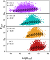 |
Fig. 9. K3 μm for K13 QSOs binned according to their redshift. Black circles give their median values over bins of width 0.2 dex. Each panel shows the QSO redshift range and the coefficient derived via a Spearman correlation test. |
In Fig. 10 we further examine the evolution of L3 μm by plotting log(L3μm/L5100 Å) versus L5100 Å. There is a clear trend showing the L3μm/L5100 Å ratio decreasing as the primary emission (i.e., L5100 Å) increases with a Spearman correlation coefficient ρ = 0.37. We fit the K13 data according to the model
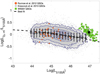 |
Fig. 10. L5100 Å vs. log(L3μm/L5100 Å). QSOs from K13 are included in the plot as gray dots, and their median values over bins of width 0.15 dex are portrayed as black circles. The black dashed line gives the best fit obtained assuming the function described in Sect. 5.4.2. WISSH QSOs are depicted as green squares; the black square shows their median value. |
which is the same function adopted by Maiolino et al. (2007), and we find A = 1.89 ± 0.01 and γ = 0.25 ± 0.01. Our fit is plotted as a dashed black line in Fig. 10. We also note a slight change in trend for L5100 Å ≈ 1046.5 erg s−1, as expected based on the analysis of the 5100 Å and the 3 μm bolometric corrections. However, this variation of trend is somewhat less evident than in the case of K3 μm.
Finally, we note that WISSH QSOs differentiate from the general distribution, being located on average 0.3 dex above the best-fit curve. Again, we observe that the separation from the bulk of the population decreases strongly as luminosity increases, and few brightest sources are in agreement with the fitted curve.
5.5. BAL versus non-BAL mean SED
Quasi-stellar objects with BALs in their rest-frame UV spectra represent about 10−20% of the total AGN population at z ∼ 2 − 4 (e.g., Gibson et al. 2009). These absorption troughs are believed to trace wind on the accretion disk scale (e.g., Hewett & Foltz 2003). It is still debated to what extent these winds are present among AGN. A first scenario assumes that all AGN have winds, but that they are ejected equatorially with a small covering factor (e.g., Elvis 2000). In this case an object is recognized as a BAL only when the line of sight intercepts the outflow. Alternatively, BAL winds could be a feature of only a fraction of the AGN population with peculiar properties, probably associated with a precise AGN evolutionary phase (e.g., Wang et al. 2016; Chen et al. 2022). In any case, whether it is an effect of the viewing angle or due to a distinct evolutionary stage, we expect BAL SEDs to differ from those of non-BAL sources. For this reason we derive and compare the composite SEDs of BAL and non-BAL subsamples among the WISSH QSOs.
For the classification of BAL sources we refer to Bruni et al. (2019). In detail, we classify as BAL those sources with a modified absorption index A1000 > 0 (34 QSOs). In the computation of the mean SED we used only the X-ray luminosity of the sources observed (13 BAL and 30 non-BAL QSOs). This choice allows us to compare only observed fluxes without assuming any correlation between the UV and X-ray regions of the SED. Furthermore, since possible dust extinction is one of the phenomena that we are most interested in, we did not remove red objects with αopt < 0.2, as was done in Sect. 4.1. However, we maintained the gap repair performed on photometry with strong absorption features in order to be sure that any differences between the SEDs are not attributable to the overlapping of the filters bandpasses with the absorption troughs. We present the comparison between the mean SEDs of BAL and non-BAL subsamples in Fig. 11, while the derived templates are reported in Table 4.
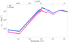 |
Fig. 11. Comparison between the mean SEDs of BAL QSOs (pink dotted line) and non-BAL QSOs (blue solid line) together with a 68% confidence interval shown as shaded area. The SEDs are not normalized. |
The main differences we find are in the X-rays and in the optical and UV region (1000 Å < λ < 1 μm). In particular, BAL QSOs are X-ray weaker (BALs SED is ∼0.3 dex less luminous) and show a redder UV-optical continuum compared to non-BAL sources.
While the difference in the X-ray seems to be intrinsic, as already found by previous works (e.g., Brandt et al. 2000; Gallagher et al. 2002, 2007b; Fan et al. 2009; Luo et al. 2014), in the optical and UV band, the redder BAL SED is instead explained as the result of a higher dust extinction (see also Reichard et al. 2003; Trump et al. 2006; Gallagher et al. 2007b; Dai et al. 2008; Krawczyk et al. 2015; Gaskell et al. 2016). This is also in agreement with redder WISE W1 − W2 colors (rest frame optical bands) in z ∼ 6 BAL quasars with respect to non-BALs found by Bischetti et al. (2022).
The WISSH BAL QSOs show flatter UV emission, which can be seen from the distribution of the optical slope αopt for BAL and non-BAL shown in the top panel of Fig. 12. According to the Kolmogorov–Smirnov (K-S) test the two samples are not drawn from the same probability distribution with a p-value of 0.0016. Assuming the same intrinsic emission, this difference can be interpreted entirely as dust extinction. The average EB − V derived in Sect. 5.4.1 is slightly higher for BAL objects (0.08 compared to 0.03 for non-BAL sources); furthermore, computing the optical slopes with intrinsic luminosities leads to compatible distributions.
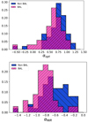 |
Fig. 12. Normalized distributions of optical and NIR spectral slopes for BAL (pink) and non-BAL (blue) sources. Top panel: normalized histograms of optical spectral slopes between 3000 Å and 1 μm. Bottom panel: normalized histograms of NIR spectral slopes between 1 μm and 4 μm. |
Moving to longer wavelengths (λ > 1 μm), the differences between the two SEDs are less evident: their emission is similar at λ > 3 μm, but BAL SED has a steeper NIR slope (1 < λ/μm < 3, αNIR(BAL) = − 0.75 ± 0.1, αNIR(non-BAL) = − 0.47 ± 0.08), as shown for individual QSOs in the bottom panel of Fig. 12. Given the higher EB − V, we would have expected more reprocessed radiation. As an example, assuming a dust covering factor of 4π and an EB − V = 0.07, we would expect BAL to be ∼43% IR brighter compared to non-BAL QSOs (see, e.g., Gallagher et al. 2007b). In the case of the analyzed WISSH sample we do not note this IR excess. However, the higher steepness in the NIR indicates a larger contribution by hot dust. Performing a K-S test on the distribution of the NIR slopes of BAL and non-BAL QSOs we find that the two samples are not drawn from the same distribution with a p-value of 0.0018.
Similarly, Zhang et al. (2014) found a small but significant correlation between the NIR slope and the BAL parameters such as the blueshifted velocity and the balnicity index. To explain the existence of these relationships, they suggested the presence of a dust component within the outflowing gas. This dust can be co-spatial with the gas clouds, and therefore be originally mixed with the outflow or it could be intercepted by the outflow once it interacts with the innermost regions of the torus. In both cases, the effect is a steepening of the NIR slope. In the first case this is due simply because outflows are believed to originate very close to the accretion disk, and the dust grains there could heat up to very high temperatures. In this case, hydrodynamical simulations showed that the effect of the powerful wind impacting dense clouds is to break them into diffuse warm filaments. In this way more dust is directly exposed to the central UV source, and is therefore heated to higher temperature.
5.6. Mean SEDs based on CIV REW
The CIV line at 1549 Å, like other high ionization lines such as SiIV and [OIII], can show a broad asymmetric profile and be blue-shifted with respect to the systemic redshift; this can be explained by assuming that the emitting region is moving toward the observer. For this reason, this line is widely studied as a tracer of outflows on the broad-line region scale. Moreover, it is observed that CIV line and especially its relative strength, expressed through the rest frame equivalent width (REW), is linked to several of the AGN properties. The best known relationship is the Baldwin effect, which is the anti-correlation between the 1550 Å luminosity and the CIV REW (Baldwin 1977). First observed on a sample of 20 sources, this relation has been confirmed with significantly larger samples (e.g., Wu et al. 2009; Richards et al. 2011), although some authors (Baskin & Laor 2004; Shemmer & Lieber 2015) suggest that it is a secondary effect and that REWCIV primarily (anti)correlates with the Eddington ratio. Under this hypothesis, a higher L/LEDD value would produce a more UV-peaked SED (Shemmer & Lieber 2015), decreasing the number of ionizing photons.
To test and analyze any possible difference between objects with different REWCIV, we derived the composite SEDs by dividing WISSH QSOs according to their REWCIV. We tried to make the subsample with lower REW to be representative of the weak line quasars (WLQs, Fan et al. 1999; Diamond-Stanic et al. 2009), a population of objects that shows the highest measured blueshifts of the lines, and is therefore associated with the fastest winds (e.g., Wu et al. 2011; Luo et al. 2015). WLQs are usually defined by having REW < 10 Å (e.g., Shemmer et al. 2009). According to Shen et al. (2011), to whom we refer for the REW measures, only three WISSH quasars satisfy this criterion and can be considered WLQSs. However, Vietri et al. (2018) found that WISSH QSOs with REWCIV < 20 Å show outflow velocities comparable with those of proper weak line emitters, suggesting that in case of particularly bright quasars, the threshold could be extended to include these sources as well.
In the construction of the composite SEDs based on CIV REWs, we softened the selection criteria even more in order to have two subsamples, both with a sufficient number of elements: 29 QSOs with REWCIV ≤ 25 Å and 56 with REWCIV > 25 Å (instead of 17 QSOs with REWCIV ≤ 20 Å and 68 with REWCIV > 20 Å). Although quasars with higher blueshifts corresponding to smaller REW are usually found to have deeper absorption troughs (Rankine et al. 2020), we note that in our sample this is not generally valid; only six sources are classified as both BAL and weaker CIV emitters (∼21% of BALs). To derive the mean SEDs we used the photometry described in Sect. 5.5. The comparison between the SEDs is presented in Fig. 13 and the derived templates are provided in Table 4.
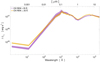 |
Fig. 13. Comparison between the mean SEDs of QSOs with REW < 25 Å (purple dotted line) and those with REW ≥ 25 Å (yellow solid line) together with a 68% confidence interval shown as the shaded area. The SEDs are not normalized. |
The main differences between the two SEDs lie in the X-ray region where QSOs with a weaker CIV line have a lower emission of about 0.4 dex. This result is in agreement with several previous works (e.g., Wu et al. 2009; Richards et al. 2011; Kruczek et al. 2011; Timlin et al. 2020; Zappacosta et al. 2020, but see also Lusso et al. 2021) and is also expressed in terms of a steeper αOX. In the UV part of our mean SEDs, we do not find strong evidence of the Baldwin effect. The CIV weak composite SED is indeed slightly more luminous in the UV, but the SEDs are compatible within the uncertainties. Performing a Spearman correlation test on the intrinsic L1550 Å and REWCIV for each individual QSO returns a null hypothesis probability (i.e., no correlation exists) with a p-value of 0.47. This result suggests that the lack of evidence of the Baldwin effect in the mean SEDs does not depend on the chosen REWCIV cut for splitting sample, but more likely on the fact that we are studying sources already at the bright end of optical luminosity function, and thus little variance among them is expected (see also the discussion in Sect. 4.4 of Lusso et al. 2021).
Moving to the IR region, we find no significant difference between the SEDs. This is in contrast with a recent work by Temple et al. (2021; but see also Wang et al. 2013) who, analyzing a sample of ∼5000 QSOs at z ≈ 2 and Lbol ∼ 1047 erg s−1, found a negative correlation between the NIR spectral slope (giving the hot dust to nuclear emission ratio) and the CIV REW. Even investigating the spectral slopes individually (Fig. 14), we do not find evidence for a difference between the two distributions. A K-S test indeed returns a null hypothesis with a p-value of 0.83.
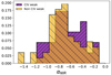 |
Fig. 14. Normalized distributions of NIR spectral slopes αNIR for QSOs with REWCIV < 25 Å (purple) and those with REWCIV ≥ 25 Å (yellow). |
5.7. SF versus AGN dominated sources
In a recent work, Symeonidis & Page (2021) studied the evolution with redshift of the fraction of AGN dominated sources for a given value of the IR 8 − 1000 μm integrated luminosity LIR. Assuming that galaxies are totally AGN powered or SF powered, this fraction is given by ℱ, defined as the ratio between the AGN IR luminosity function ϕAGN, derived from the X-ray luminosity function by Aird et al. (2015), and the galaxy IR luminosity function ϕgal by Gruppioni et al. (2013).
Defining as L25(z) and L75(z) the luminosity values for which ℱ is respectively 0.25 and 0.75, Symeonidis & Page (2021) defined three regions in the z − LIR space: the AGN dominated region for sources with LIR > L75, the transition region for those with L25 ≤ LIR ≤ L75, and the star formation dominated region for galaxies with LIR < L25. As can be seen in Fig. 15, the IR luminosity required to be in the AGN dominated region increases with z. Moreover, Symeonidis & Page (2021) filled this z − LIR diagram with quasar samples taken from various catalogs (including about half of the WISSH QSOs), each claiming to contain the brightest QSOs for a given range of redshift. Being very luminous, almost all these sources are located in the AGN dominated region (see Fig. 8 from their work).
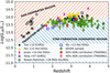 |
Fig. 15. [Adapted from Fig. 8 in Symeonidis & Page (2021)]. Redshift vs. L8 − 1000 μm diagram partitioned into an AGN dominated region, a transition region, and a star formation dominated region. Overplotted are various samples from the literature: the IRAS-selected HyLIRGs from Rowan-Robinson et al. (2018), the intermediate redshift ULIRGs from Yang et al. (2007), the optically unobscured QSOs from Tsai et al. (2015), and the hot dust obscured galaxies (hot DOGs) from Fan et al. (2016), Jones et al. (2014), and Wu et al. (2012). The WISSH quasars studied in this work are shown as green squares. Symbols with an “x” inside represent QSOs with FIR ALMA/NOEMA coverage. Plotted as red squares are WISSH08 and WISSH51, for which Duras et al. (2017) evaluated the AGN contribution to LIR. |
We added the whole WISSH sample to this diagram. The WISSH LIR values were derived using the same procedure discussed in Sect. 5.4.1, but in this case we limited the fit to WISE, Herschel and ALMA, or NOEMA photometry and fixed the EB − V to the already computed value. We expect to get the more accurate LIR estimates for sources with measured ALMA/NOEMA fluxes; these observations, in addition to providing a better sampling of the integration interval, are high-resolution and spatially resolved (i.e., the measured emission comes exclusively from the active galaxy and is not affected by the possible presence of a nearby companion).
When included in the z − LIR diagram, almost all WISSH sources (∼88%) up to z ∼ 3.5 are in agreement with the proposed partition, being either in the AGN dominated region or in the transition region (see Fig. 15). However, this percentage drops to ∼50% at z > 3.5. Although, as clearly stated by Symeonidis & Page (2021), this z − LIR diagram should not be used as a precise diagnostic instrument, and it could happen that AGN dominated sources fall in the starbust region, and conversely, it would seem that despite their high luminosities the FIR emission of WISSH QSOs at z ∼ 3.5 is still mostly powered by star formation activity. This conclusion is supported by Bischetti et al. (2021) who found WISSH QSOs to be located in high star-forming environments. On the other hand, our findings disagree with those by Symeonidis et al. (2022) who determined that, for QSOs with L5100 Å ≳ 1046 erg s−1, LIR essentially traces the AGN primary emission and that the contribution provided by SF becomes almost negligible. However, although their results in the high-luminosity regime seem to be redshift independent, the sample studied by Symeonidis et al. (2022) consists only of QSOs up to z = 2.65. Furthermore, our conclusions depend (mostly) on the diagram partition. It should be remembered that in the original z − LIR diagram, ℱ was computed by Symeonidis & Page (2021) only up to z = 2.5 and then extrapolated up to z = 4 based on the evolution of ϕgal (and we extrapolated up to z = 5 to include all WISSH QSOs, moving farther away from the region constrained by observations). The reason behind this choice is the severe lack of spectroscopic redshifts among the population that makes up the IR luminosity function at z > 2.5 (Symeonidis & Page 2021). As a result, the possibility that our findings are influenced by the fact that we are looking at a portion of the diagram where the partition is rather uncertain cannot be ruled out. As a partially independent test for the proposed partition, we took into account results by Duras et al. (2017) who, using the radiative transfer code TRADING (Bianchi 2008) on WISSH08 and WISSH51 (i.e., the two QSOs with the highest and lowest luminosity as measured by Herschel), established the AGN contribution to LIR to be respectively 60% and 40%. By looking at the placement of these two QSOs in the diagram, we find that they are located in the transition region, and are thus in agreement with the independently computed AGN contribution. Unfortunately, these sources have z = 3.23 and z = 2.89, and so they only marginally test the high-redshift region, which is the one we are most interested in.
6. Summary and conclusions
In this work we derived the mean SED of the WISSH sample: 85 hyperluminous type 1 QSOs. Our results can be summarized as follows:
-
Overall, the shape of the mean SED of these sources is very similar to that of the bulk of the type 1 quasar population. The main differences are observed in the X-ray region where WISSH quasars are weaker, and in the near- and mid-IR bands where instead they show an excess in their emission. This excess is responsible for a more prominent red bump and for the shifting of the SED dip from 1.3 to 1.1 μm.
-
The IR excess has been previously reported in the literature and can be explained by assuming an extra contribution from dust. We find that to properly model this IR excess two distinct dust components are required: warm dust (T ≈ 450 − 800 K), probably associated with the torus and responsible for the enhancement of the IR bump longward of ∼3 μm, and hot dust close to the sublimation temperature (T > 1000 K), which accounts for the divergences at λ ∼ 1 − 3 μm. Further investigations are needed to confirm both the shift of the dip and the origin of this extra hot dust contribution that we are unable to explain in the context of classical AGN models.
-
The lower X-ray emission is an already well-known feature of luminous QSOs, and it is in agreement with the αOX − lUV anti-correlation (e.g., Vignali et al. 2003; Lusso et al. 2010; Martocchia et al. 2017).
-
By modeling the QSOs emission with the mean SED and integrating it between 10 keV and 1 μm, we computed the bolometric luminosities, confirming that WISSH quasars are indeed among the most luminous AGN, having Lbol > 1047 erg s−1. By combining Lbol with the monochromatic luminosities, we then derived the 5100 Å and 3 μm bolometric corrections. We compared our results with data by Runnoe et al. (2012a) and K13. In the case of K5100 Å, WISSH QSOs have a similar distribution to that of lower luminosity QSOs, and are in agreement with the relationships proposed by Runnoe et al. (2012a) and K13. For λ = 3 μm we observe in WISSH QSOs a lower bolometric correction than in the bulk of the population. We also derived a new luminosity-dependent K3 μm described by a piecewise function (i.e., with an increasing trend up to Lbol ≈ 1047 erg s−1) followed by a slightly decreasing function at higher luminosities.
-
An increasing K3 μm versus Lbol is in agreement with Maiolino et al. (2007), who interpreted this trend as being due to a decrease in torus covering factor with increasing luminosities. However, the observed high-luminosity change in the K3 μm trend might indicate a limiting radius beyond which an increase in the primary emission does not correspond to a further receding of the torus, but rather to an increment of dust heated up to its sublimation temperature. This would be in agreement with what is found in the WISSH mean SED.
We also derived the mean SEDs by splitting the sample according to their spectral features: BAL versus non-BAL and REWCIV ≤ 25 Å versus REWCIV > 25 Å. We find the following:
-
BALs exhibits lower X-ray emission and a depressed UV to optical continuum. The X-ray weakness is usually considered intrinsic since it is present even when luminosities are corrected for the absorption; the flatter UV-optical spectrum is instead compatible with a larger extinction by dust. We also note that BALs have a steeper NIR slope, which indicates a higher contribution by the hottest dust component; this result is in agreement with the analysis by Zhang et al. (2014).
-
We find a clear dichotomy between the CIV weak and non-weak populations regarding their X-ray emission. QSOs with a smaller equivalent width have an intrinsic lower X-ray emission. This result is consistent with the already known REWCIV – X-ray correlation. As in the case of BALs, the lower X-ray output from weaker CIV emitters seems to be intrinsic. For our quasars the Baldwin effect is not evident enough to appreciate its effect, neither in the comparison between the mean SEDs nor when investigating the individual quasar SEDs. We also do not find any evidence for the REWCIV and NIR spectral slope correlation which was recently suggested by Temple et al. (2021).
Finally, we included the WISSH quasars in the z − LIR diagram by Symeonidis & Page (2021), which explores the evolution with redshift of the fraction of AGN dominated versus SF dominated sources. We find that up to z ∼ 3.5, ∼88% of WISSH QSOs fall either in the AGN dominated or transition region, while this percentage drops below 50% for higher redshifts. This last finding would suggest that even QSOs specifically selected to be the most luminous have FIR emission mostly dominated by SF activity. In any case, this result relies on the strong and nontrivial assumption that the partition proposed by Symeonidis & Page (2021) still holds for z > 3.5, which we cannot prove, and therefore we are unable to draw any firm conclusions.
Concluding, the mean SED of extremely luminous WISSH QSOs exhibits non-negligible differences compared to that of less luminous sources. These differences are likely also present in other samples of hyperluminous quasars, such as those in the high-z Universe (z > 6.5; e.g., Mazzucchelli et al. 2017). For this reason, in the analysis of the latter we recommend using SED templates specifically constructed from very luminous QSOs.
These values should be taken as purely indicative as in reality we expect a gradient of temperatures.
The K5100 Å reported by K13 was derived assuming 1 μm and 2 keV as integration limits for Lbol. Including also the 2−10 keV luminosity, we derived K5100 Å = 4.80 ± 1.54, which is the value shown in Fig. 8 as a dot-dashed black line.
Acknowledgments
We are grateful to the anonymous referee for their useful comments and suggestions which helped us to improve the paper. I.S. thanks Coleman. M. Krawczyk for providing helpful advice on the derivation of the mean SED. I.S. also thanks Myrto Symeonidis for providing LIR data. M.B. and E.P. acknowledge support from PRIN MIUR project “Black Hole winds and the Baryon Life Cycle of Galaxies: the stone-guest at the galaxy evolution supper”, contract #2017PH3WAT. R.M. acknowledges support by the Science and Technology Facilities Council (STFC) and ERC Advanced Grant 695671 “QUENCH”. R.M. also acknowledges funding from a research professorship from the Royal Society.
References
- Aird, J., Coil, A. L., Georgakakis, A., et al. 2015, MNRAS, 451, 1892 [Google Scholar]
- Andrae, R. 2010, arXiv e-prints [arXiv:1009.2755] [Google Scholar]
- Baldwin, J. A. 1977, ApJ, 214, 679 [NASA ADS] [CrossRef] [Google Scholar]
- Baldwin, J. A., Wampler, E. J., & Gaskell, C. M. 1989, ApJ, 338, 630 [NASA ADS] [CrossRef] [Google Scholar]
- Baskin, A., & Laor, A. 2004, MNRAS, 350, L31 [NASA ADS] [CrossRef] [Google Scholar]
- Bian, W.-H., Fang, L.-L., Huang, K.-L., & Wang, J.-M. 2012, MNRAS, 427, 2881 [NASA ADS] [CrossRef] [Google Scholar]
- Bianchi, S. 2008, A&A, 490, 461 [NASA ADS] [CrossRef] [EDP Sciences] [Google Scholar]
- Bianchini, F., Fabbian, G., Lapi, A., et al. 2019, ApJ, 871, 136 [CrossRef] [Google Scholar]
- Bischetti, M., Piconcelli, E., Vietri, G., et al. 2017, A&A, 598, A122 [NASA ADS] [CrossRef] [EDP Sciences] [Google Scholar]
- Bischetti, M., Piconcelli, E., Feruglio, C., et al. 2018, A&A, 617, A82 [NASA ADS] [CrossRef] [EDP Sciences] [Google Scholar]
- Bischetti, M., Maiolino, R., Carniani, S., et al. 2019, A&A, 630, A59 [NASA ADS] [CrossRef] [EDP Sciences] [Google Scholar]
- Bischetti, M., Feruglio, C., Piconcelli, E., et al. 2021, A&A, 645, A33 [NASA ADS] [CrossRef] [EDP Sciences] [Google Scholar]
- Bischetti, M., Feruglio, C., D’Odorico, V., et al. 2022, Nature, 605, 244 [NASA ADS] [CrossRef] [Google Scholar]
- Blandford, R. D., & Payne, D. G. 1982, MNRAS, 199, 883 [CrossRef] [Google Scholar]
- Bongiorno, A., Merloni, A., Brusa, M., et al. 2012, MNRAS, 427, 3103 [Google Scholar]
- Brandt, W. N., Laor, A., & Wills, B. J. 2000, ApJ, 528, 637 [CrossRef] [Google Scholar]
- Bruni, G., Piconcelli, E., Misawa, T., et al. 2019, A&A, 630, A111 [NASA ADS] [CrossRef] [EDP Sciences] [Google Scholar]
- Bussmann, R. S., Riechers, D., Fialkov, A., et al. 2015, ApJ, 812, 43 [Google Scholar]
- Calderone, G., Sbarrato, T., & Ghisellini, G. 2012, MNRAS, 425, L41 [NASA ADS] [CrossRef] [Google Scholar]
- Caplar, N., Lilly, S. J., & Trakhtenbrot, B. 2017, ApJ, 834, 111 [NASA ADS] [CrossRef] [Google Scholar]
- Casebeer, D. A., Leighly, K. M., & Baron, E. 2006, ApJ, 637, 157 [NASA ADS] [CrossRef] [Google Scholar]
- Chen, Z., He, Z., Ho, L. C., et al. 2022, Nat. Astron., 6, 339 [NASA ADS] [CrossRef] [Google Scholar]
- Cicone, C., Maiolino, R., Sturm, E., et al. 2014, A&A, 562, A21 [NASA ADS] [CrossRef] [EDP Sciences] [Google Scholar]
- Dai, X., Shankar, F., & Sivakoff, G. R. 2008, ApJ, 672, 108 [NASA ADS] [CrossRef] [Google Scholar]
- Diamond-Stanic, A. M., Fan, X., Brandt, W. N., et al. 2009, ApJ, 699, 782 [NASA ADS] [CrossRef] [Google Scholar]
- Duras, F., Bongiorno, A., Piconcelli, E., et al. 2017, A&A, 604, A67 [NASA ADS] [CrossRef] [EDP Sciences] [Google Scholar]
- Duras, F., Bongiorno, A., Ricci, F., et al. 2020, A&A, 636, A73 [NASA ADS] [CrossRef] [EDP Sciences] [Google Scholar]
- Elvis, M. 2000, ApJ, 545, 63 [NASA ADS] [CrossRef] [Google Scholar]
- Elvis, M., Wilkes, B. J., McDowell, J. C., et al. 1994, ApJS, 95, 1 [Google Scholar]
- Fan, X., Strauss, M. A., Gunn, J. E., et al. 1999, ApJ, 526, L57 [NASA ADS] [CrossRef] [Google Scholar]
- Fan, L. L., Wang, H. Y., Wang, T., et al. 2009, ApJ, 690, 1006 [NASA ADS] [CrossRef] [Google Scholar]
- Fan, L., Han, Y., Nikutta, R., Drouart, G., & Knudsen, K. K. 2016, ApJ, 823, 107 [Google Scholar]
- Fiore, F., Feruglio, C., Shankar, F., et al. 2017, A&A, 601, A143 [NASA ADS] [CrossRef] [EDP Sciences] [Google Scholar]
- Fluetsch, A., Maiolino, R., Carniani, S., et al. 2019, MNRAS, 483, 4586 [NASA ADS] [Google Scholar]
- Gallagher, S. C., Brandt, W. N., Chartas, G., & Garmire, G. P. 2002, ApJ, 567, 37 [CrossRef] [Google Scholar]
- Gallagher, S. C., Richards, G. T., Lacy, M., et al. 2007a, ApJ, 661, 30 [NASA ADS] [CrossRef] [Google Scholar]
- Gallagher, S. C., Hines, D. C., Blaylock, M., et al. 2007b, ApJ, 665, 157 [NASA ADS] [CrossRef] [Google Scholar]
- Gaskell, C. M., Gill, J. J. M., & Singh, J. 2016, MNRAS, submitted [arXiv:1611.03733] [Google Scholar]
- Gibson, R. R., Jiang, L., Brandt, W. N., et al. 2009, ApJ, 692, 758 [Google Scholar]
- Glikman, E., Gregg, M. D., Lacy, M., et al. 2004, ApJ, 607, 60 [NASA ADS] [CrossRef] [Google Scholar]
- Glikman, E., Lacy, M., LaMassa, S., et al. 2022, ApJ, 934, 119 [NASA ADS] [CrossRef] [Google Scholar]
- Gruppioni, C., Pozzi, F., Polletta, M., et al. 2008, ApJ, 684, 136 [NASA ADS] [CrossRef] [Google Scholar]
- Gruppioni, C., Pozzi, F., Rodighiero, G., et al. 2013, MNRAS, 432, 23 [Google Scholar]
- Gu, M. 2013, ApJ, 773, 176 [NASA ADS] [CrossRef] [Google Scholar]
- Hao, H., Elvis, M., Civano, F., et al. 2014, MNRAS, 438, 1288 [Google Scholar]
- Hasinger, G., Miyaji, T., & Schmidt, M. 2005, A&A, 441, 417 [NASA ADS] [CrossRef] [EDP Sciences] [Google Scholar]
- Hatziminaoglou, E., Pérez-Fournon, I., Polletta, M., et al. 2005, AJ, 129, 1198 [NASA ADS] [CrossRef] [Google Scholar]
- Hatziminaoglou, E., Farrah, D., Humphreys, E., et al. 2018, MNRAS, 480, 4974 [Google Scholar]
- Hernán-Caballero, A., Hatziminaoglou, E., Alonso-Herrero, A., & Mateos, S. 2016, MNRAS, 463, 2064 [Google Scholar]
- Hewett, P. C., & Foltz, C. B. 2003, AJ, 125, 1784 [NASA ADS] [CrossRef] [Google Scholar]
- Hewett, P. C., & Wild, V. 2010, MNRAS, 405, 2302 [NASA ADS] [Google Scholar]
- Inoue, A. K., Shimizu, I., Iwata, I., & Tanaka, M. 2014, MNRAS, 442, 1805 [NASA ADS] [CrossRef] [Google Scholar]
- Ishibashi, W., & Fabian, A. C. 2012, MNRAS, 427, 2998 [NASA ADS] [CrossRef] [Google Scholar]
- Jones, S. F., Blain, A. W., Stern, D., et al. 2014, MNRAS, 443, 146 [Google Scholar]
- Kakkad, D., Mainieri, V., Vietri, G., et al. 2020, A&A, 642, A147 [NASA ADS] [CrossRef] [EDP Sciences] [Google Scholar]
- Korista, K., Ferland, G., & Baldwin, J. 1997, ApJ, 487, 555 [NASA ADS] [CrossRef] [Google Scholar]
- Krawczyk, C. M., Richards, G. T., Mehta, S. S., et al. 2013, ApJS, 206, 4 [Google Scholar]
- Krawczyk, C. M., Richards, G. T., Gallagher, S. C., et al. 2015, AJ, 149, 203 [NASA ADS] [CrossRef] [Google Scholar]
- Kruczek, N. E., Richards, G. T., Gallagher, S. C., et al. 2011, AJ, 142, 130 [NASA ADS] [CrossRef] [Google Scholar]
- Lawrence, A. 1991, MNRAS, 252, 586 [NASA ADS] [Google Scholar]
- Liang, E. P. T., & Thompson, K. A. 1979, MNRAS, 189, 421 [NASA ADS] [Google Scholar]
- Luo, B., Brandt, W. N., Alexander, D. M., et al. 2014, ApJ, 794, 70 [Google Scholar]
- Luo, B., Brandt, W. N., Hall, P. B., et al. 2015, ApJ, 805, 122 [Google Scholar]
- Lusso, E., Comastri, A., Vignali, C., et al. 2010, A&A, 512, A34 [NASA ADS] [CrossRef] [EDP Sciences] [Google Scholar]
- Lusso, E., Comastri, A., Simmons, B. D., et al. 2012, MNRAS, 425, 623 [Google Scholar]
- Lusso, E., Hennawi, J. F., Comastri, A., et al. 2013, ApJ, 777, 86 [Google Scholar]
- Lusso, E., Worseck, G., Hennawi, J. F., et al. 2015, MNRAS, 449, 4204 [Google Scholar]
- Lusso, E., Nardini, E., Bisogni, S., et al. 2021, A&A, 653, A158 [NASA ADS] [CrossRef] [EDP Sciences] [Google Scholar]
- Lutz, D., Sturm, E., Janssen, A., et al. 2020, A&A, 633, A134 [NASA ADS] [CrossRef] [EDP Sciences] [Google Scholar]
- Lyke, B. W., Higley, A. N., McLane, J. N., et al. 2020, ApJS, 250, 8 [NASA ADS] [CrossRef] [Google Scholar]
- Lynden-Bell, D. 1969, Nature, 223, 690 [NASA ADS] [CrossRef] [Google Scholar]
- Lyu, J., & Rieke, G. H. 2018, ApJ, 866, 92 [Google Scholar]
- Ma, X.-C., & Wang, T.-G. 2013, MNRAS, 430, 3445 [NASA ADS] [CrossRef] [Google Scholar]
- Madau, P., & Dickinson, M. 2014, ARA&A, 52, 415 [Google Scholar]
- Maiolino, R., Shemmer, O., Imanishi, M., et al. 2007, A&A, 468, 979 [NASA ADS] [CrossRef] [EDP Sciences] [Google Scholar]
- Marconi, A., Risaliti, G., Gilli, R., et al. 2004, MNRAS, 351, 169 [Google Scholar]
- Martocchia, S., Piconcelli, E., Zappacosta, L., et al. 2017, A&A, 608, A51 [NASA ADS] [CrossRef] [EDP Sciences] [Google Scholar]
- Mathews, W. G., & Ferland, G. J. 1987, ApJ, 323, 456 [NASA ADS] [CrossRef] [Google Scholar]
- Mazzucchelli, C., Bañados, E., Venemans, B. P., et al. 2017, ApJ, 849, 91 [Google Scholar]
- Nemmen, R. S., & Brotherton, M. S. 2010, MNRAS, 408, 1598 [Google Scholar]
- Pâris, I., Petitjean, P., Aubourg, É., et al. 2014, A&A, 563, A54 [NASA ADS] [CrossRef] [EDP Sciences] [Google Scholar]
- Piconcelli, E., Jimenez-Bailón, E., Guainazzi, M., et al. 2005, A&A, 432, 15 [NASA ADS] [CrossRef] [EDP Sciences] [Google Scholar]
- Pogge, R. W., & Peterson, B. M. 1992, AJ, 103, 1084 [NASA ADS] [CrossRef] [Google Scholar]
- Prevot, M. L., Lequeux, J., Maurice, E., Prevot, L., & Rocca-Volmerange, B. 1984, A&A, 132, 389 [Google Scholar]
- Rankine, A. L., Hewett, P. C., Banerji, M., & Richards, G. T. 2020, MNRAS, 492, 4553 [CrossRef] [Google Scholar]
- Reichard, T. A., Richards, G. T., Hall, P. B., et al. 2003, AJ, 126, 2594 [NASA ADS] [CrossRef] [Google Scholar]
- Richards, G. T., Lacy, M., Storrie-Lombardi, L. J., et al. 2006, ApJS, 166, 470 [Google Scholar]
- Richards, G. T., Kruczek, N. E., Gallagher, S. C., et al. 2011, AJ, 141, 167 [Google Scholar]
- Ross, N. P., Hamann, F., Zakamska, N. L., et al. 2015, MNRAS, 453, 3932 [Google Scholar]
- Rowan-Robinson, M., Wang, L., Farrah, D., et al. 2018, A&A, 619, A169 [NASA ADS] [CrossRef] [EDP Sciences] [Google Scholar]
- Runnoe, J. C., Brotherton, M. S., & Shang, Z. 2012a, MNRAS, 422, 478 [Google Scholar]
- Runnoe, J. C., Brotherton, M. S., & Shang, Z. 2012b, MNRAS, 426, 2677 [NASA ADS] [CrossRef] [Google Scholar]
- Schlafly, E. F., & Finkbeiner, D. P. 2011, ApJ, 737, 103 [Google Scholar]
- Scott, J. E., Kriss, G. A., Brotherton, M., et al. 2004, ApJ, 615, 135 [NASA ADS] [CrossRef] [Google Scholar]
- Shang, Z., Brotherton, M. S., Wills, B. J., et al. 2011, ApJS, 196, 2 [Google Scholar]
- Shemmer, O., & Lieber, S. 2015, ApJ, 805, 124 [NASA ADS] [CrossRef] [Google Scholar]
- Shemmer, O., Brandt, W. N., Anderson, S. F., et al. 2009, ApJ, 696, 580 [NASA ADS] [CrossRef] [Google Scholar]
- Shen, Y., Richards, G. T., Strauss, M. A., et al. 2011, ApJS, 194, 45 [Google Scholar]
- Siebenmorgen, R., Haas, M., Krügel, E., & Schulz, B. 2005, A&A, 436, L5 [NASA ADS] [CrossRef] [EDP Sciences] [Google Scholar]
- Simpson, C. 2005, MNRAS, 360, 565 [NASA ADS] [CrossRef] [Google Scholar]
- Stalevski, M., Fritz, J., Baes, M., Nakos, T., & Popović, L. Č. 2012, MNRAS, 420, 2756 [Google Scholar]
- Steffen, A. T., Strateva, I., Brandt, W. N., et al. 2006, AJ, 131, 2826 [Google Scholar]
- Stevans, M. L., Shull, J. M., Danforth, C. W., & Tilton, E. M. 2014, ApJ, 794, 75 [NASA ADS] [CrossRef] [Google Scholar]
- Symeonidis, M., & Page, M. J. 2021, MNRAS, 503, 3992 [NASA ADS] [CrossRef] [Google Scholar]
- Symeonidis, M., Maddox, N., Jarvis, M. J., et al. 2022, MNRAS, 514, 4450 [CrossRef] [Google Scholar]
- Temple, M. J., Banerji, M., Hewett, P. C., Rankine, A. L., & Richards, G. T. 2021, MNRAS, 501, 3061 [Google Scholar]
- Timlin, J. D., Brandt, W. N., Ni, Q., et al. 2020, MNRAS, 492, 719 [Google Scholar]
- Trakhtenbrot, B., Lira, P., Netzer, H., et al. 2017, ApJ, 836, 8 [NASA ADS] [CrossRef] [Google Scholar]
- Travascio, A., Zappacosta, L., Cantalupo, S., et al. 2020, A&A, 635, A157 [NASA ADS] [CrossRef] [EDP Sciences] [Google Scholar]
- Trump, J. R., Hall, P. B., Reichard, T. A., et al. 2006, ApJS, 165, 1 [Google Scholar]
- Tsai, C.-W., Eisenhardt, P. R. M., Wu, J., et al. 2015, ApJ, 805, 90 [Google Scholar]
- Ueda, Y., Akiyama, M., Ohta, K., & Miyaji, T. 2003, ApJ, 598, 886 [NASA ADS] [CrossRef] [Google Scholar]
- Vanden Berk, D. E., Richards, G. T., Bauer, A., et al. 2001, AJ, 122, 549 [Google Scholar]
- Vanden Berk, D. E., Wilhite, B. C., Kron, R. G., et al. 2004, ApJ, 601, 692 [Google Scholar]
- Veilleux, S., Meléndez, M., Sturm, E., et al. 2013, ApJ, 776, 27 [Google Scholar]
- Vietri, G., Piconcelli, E., Bischetti, M., et al. 2018, A&A, 617, A81 [NASA ADS] [CrossRef] [EDP Sciences] [Google Scholar]
- Vietri, G., Mainieri, V., Kakkad, D., et al. 2020, A&A, 644, A175 [NASA ADS] [CrossRef] [EDP Sciences] [Google Scholar]
- Vignali, C., Brandt, W. N., & Schneider, D. P. 2003, AJ, 125, 433 [Google Scholar]
- Wang, H., Xing, F., Zhang, K., et al. 2013, ApJ, 776, L15 [NASA ADS] [CrossRef] [Google Scholar]
- Wang, T., Ferland, G. J., Yang, C., Wang, H., & Zhang, S. 2016, ApJ, 824, 106 [NASA ADS] [CrossRef] [Google Scholar]
- Weedman, D., Sargsyan, L., Lebouteiller, V., Houck, J., & Barry, D. 2012, ApJ, 761, 184 [Google Scholar]
- Wright, E. L., Eisenhardt, P. R. M., Mainzer, A. K., et al. 2010, ApJ, 140, 1868 [Google Scholar]
- Wu, J., Vanden Berk, D. E., Brandt, W. N., et al. 2009, ApJ, 702, 767 [NASA ADS] [CrossRef] [Google Scholar]
- Wu, J., Brandt, W. N., Hall, P. B., et al. 2011, ApJ, 736, 28 [NASA ADS] [CrossRef] [Google Scholar]
- Wu, X.-B., Hao, G., Jia, Z., Zhang, Y., & Peng, N. 2012, ApJ, 144, 49 [CrossRef] [Google Scholar]
- Yang, M., Greve, T. R., Dowell, C. D., & Borys, C. 2007, ApJ, 660, 1198 [NASA ADS] [CrossRef] [Google Scholar]
- Yang, G., Boquien, M., Brandt, W. N., et al. 2022, ApJ, 927, 192 [NASA ADS] [CrossRef] [Google Scholar]
- Yi, W., Zuo, W., Yang, J., et al. 2020, ApJ, 893, 95 [NASA ADS] [CrossRef] [Google Scholar]
- Zappacosta, L., Piconcelli, E., Giustini, M., et al. 2020, A&A, 635, L5 [NASA ADS] [CrossRef] [EDP Sciences] [Google Scholar]
- Zhang, S., Wang, H., Wang, T., et al. 2014, ApJ, 786, 42 [NASA ADS] [CrossRef] [Google Scholar]
- Zheng, W., Kriss, G. A., Telfer, R. C., Grimes, J. P., & Davidsen, A. F. 1997, ApJ, 475, 469 [NASA ADS] [CrossRef] [Google Scholar]
Appendix A: TNG data reduction
The near-IR data were collected during program A37TAC_32 in period 37 and program A42TAC_17 in period 42 (PI: V. Testa). The reduction was performed following a standard procedure currently adopted for this type of detectors: images were acquired adopting a dithering strategy, which produced nine or ten image per cycle for each filter. These images were then median stacked using a clipping algorithm to obtain an empty-sky frame, which was subtracted from all the single frames. The output of this stage is a set of images with a zero count background level. This procedure removes bias and dark current levels together with the sky, and provides a zeroth order flat-fielding. The following step was to normalize all the single frames with a flat-field image obtained using twilight sky frames as suggested on the telescope site. The flat-fielded images were then registered and co-added obtaining the final frames for each filter on which the data analysis was performed. We used a set of semi-automatic procedures using IRAF and DAOPHOT and the instrumental magnitudes were calibrated through a set of stars in the field with the 2MASS survey.
All Tables
Mean SEDs computed for the WISSH full sample and for the subsamples: BAL, non-BAL, REWCIV < 25 Å, REWCIV ≥ 25 Å.
All Figures
|
Fig. 3. Mean SED derived from the WISSH sample. The shaded area gives the 68% confidence interval. The colored circles represent available data points, color-coded according to the filter in which they were observed. Photometry obtained by Gap Repair is represented as gray circles. The gray crosses indicate X-ray luminosities reconstructed from the αOX relationship. The dotted black line indicates the Lyman limit λL = 912 Å: for shorter wavelengths the mean SED was truncated and extended as explained in Sect. 4.4. |
| In the text | |
|
Fig. 1. Example of corrections applied to take into account both IGM absorption and emission lines for WISSH23 at z = 4.4. The empty diamonds represent the observed fluxes, while the filled diamonds are the fluxes after corrections. The horizontal bars indicate the range of wavelengths covered by the filters. |
| In the text | |
|
Fig. 2. 2 keV luminosity distribution of the sample. We include both measured values (green histogram) by Martocchia et al. (2017) and Zappacosta et al. (2020) and derived values using the L2 keV − L2500 Å relation. |
| In the text | |
|
Fig. 4. Comparison between the WISSH mean SED derived in this work (black line), the overall mean SED for type 1 QSOs by K13 (light blue line), and the high-luminosity SED also by K13 (dotted red line). SEDs are normalized at 1.3 μm (dotted vertical line). The inset shows an image of the SEDs zoomed-in on the 0.7 < λ/μm < 6 range. |
| In the text | |
|
Fig. 5. Modeling of the WISSH mean SED via the K13 composite SED plus one (top panel) or two (bottom panel) modified blackbodies, as described in Sect. 5.1. A comparison of the two solid orange lines shows how the addition of a hotter dust component allows a better reproduction of the curve for λ < 2 μm. |
| In the text | |
|
Fig. 6. Best-fit and 1σ errors of the WISSH mean SED via CIGALE-generated templates. For illustrative purposes the different components considered in CIGALE and whose sum provides the overall AGN SED are plotted in different colors. The best-fit parameters are OA = 50°, τν = 11, p = 1.0, q = 0, δAD = −0.4, Rin/Rout = 20, TPD = 100 K, EB − V = 0.03 (see Yang et al. 2022, for a detailed description of these parameters). The dotted lines delimit the wavelength range over which the fitting was performed. |
| In the text | |
|
Fig. 7. Bolometric and monochromatic luminosities distributions of the WISSH sample. From left to right: Bolometric luminosities, intrinsic monochromatic luminosities at 5100 Å and 3 μm, and EB − V. |
| In the text | |
|
Fig. 8. Bolometric corrections at λ = 5100 Å and 3 μm vs. Lbol. Top panel: K5100 Å vs. Log(Lbol), in units of [erg s−1]. QSOs from Runnoe et al. (2012a) are shown as orange filled circles. Gray circles depict QSOs from Krawczyk et al. (2013), while black circles provide their median values (with the associated spread) over bins of width 0.15 dex. WISSH QSOs are shown as green squares, and the black square indicates their mean. The solid orange line describe the nonlinear relationship by Runnoe et al. (2012a), the dotted line indicates that the relation is being extrapolated to lower or higher luminosities. The dashed black lines give the linear relationship by K13 and its associated uncertainty. Bottom panel: K3 μm vs. Log(Lbol), color-coded as above. Here the dashed black lines depict the best fit computed as explained in Sect. 5.4.1 and its uncertainty computed as the square root of the variance with respect to the best-fit prediction. |
| In the text | |
|
Fig. 9. K3 μm for K13 QSOs binned according to their redshift. Black circles give their median values over bins of width 0.2 dex. Each panel shows the QSO redshift range and the coefficient derived via a Spearman correlation test. |
| In the text | |
|
Fig. 10. L5100 Å vs. log(L3μm/L5100 Å). QSOs from K13 are included in the plot as gray dots, and their median values over bins of width 0.15 dex are portrayed as black circles. The black dashed line gives the best fit obtained assuming the function described in Sect. 5.4.2. WISSH QSOs are depicted as green squares; the black square shows their median value. |
| In the text | |
|
Fig. 11. Comparison between the mean SEDs of BAL QSOs (pink dotted line) and non-BAL QSOs (blue solid line) together with a 68% confidence interval shown as shaded area. The SEDs are not normalized. |
| In the text | |
|
Fig. 12. Normalized distributions of optical and NIR spectral slopes for BAL (pink) and non-BAL (blue) sources. Top panel: normalized histograms of optical spectral slopes between 3000 Å and 1 μm. Bottom panel: normalized histograms of NIR spectral slopes between 1 μm and 4 μm. |
| In the text | |
|
Fig. 13. Comparison between the mean SEDs of QSOs with REW < 25 Å (purple dotted line) and those with REW ≥ 25 Å (yellow solid line) together with a 68% confidence interval shown as the shaded area. The SEDs are not normalized. |
| In the text | |
|
Fig. 14. Normalized distributions of NIR spectral slopes αNIR for QSOs with REWCIV < 25 Å (purple) and those with REWCIV ≥ 25 Å (yellow). |
| In the text | |
|
Fig. 15. [Adapted from Fig. 8 in Symeonidis & Page (2021)]. Redshift vs. L8 − 1000 μm diagram partitioned into an AGN dominated region, a transition region, and a star formation dominated region. Overplotted are various samples from the literature: the IRAS-selected HyLIRGs from Rowan-Robinson et al. (2018), the intermediate redshift ULIRGs from Yang et al. (2007), the optically unobscured QSOs from Tsai et al. (2015), and the hot dust obscured galaxies (hot DOGs) from Fan et al. (2016), Jones et al. (2014), and Wu et al. (2012). The WISSH quasars studied in this work are shown as green squares. Symbols with an “x” inside represent QSOs with FIR ALMA/NOEMA coverage. Plotted as red squares are WISSH08 and WISSH51, for which Duras et al. (2017) evaluated the AGN contribution to LIR. |
| In the text | |
Current usage metrics show cumulative count of Article Views (full-text article views including HTML views, PDF and ePub downloads, according to the available data) and Abstracts Views on Vision4Press platform.
Data correspond to usage on the plateform after 2015. The current usage metrics is available 48-96 hours after online publication and is updated daily on week days.
Initial download of the metrics may take a while.