| Issue |
A&A
Volume 693, January 2025
|
|
|---|---|---|
| Article Number | A157 | |
| Number of page(s) | 17 | |
| Section | Extragalactic astronomy | |
| DOI | https://doi.org/10.1051/0004-6361/202450876 | |
| Published online | 14 January 2025 | |
HYPERION: Broad-band X-ray-to-near-infrared emission of quasars in the first billion years of the Universe
1
Dipartimento di Matematica e Fisica, Università Roma Tre, Via della Vasca Navale 84, 00146 Roma, Italy
2
INAF – Osservatorio Astronomico di Roma, Via Frascati 33, I-00040 Monte Porzio Catone, Italy
3
INAF – Osservatorio Astronomico di Trieste, Via G. Tiepolo 11, I-34143 Trieste, Italy
4
Dipartimento di Fisica, Sezione di Astronomia, Università di Trieste, Via Tiepolo 11, I-34143 Trieste, Italy
5
Scuola Normale Superiore, Piazza dei Cavalieri 7, I-56126 Pisa, Italy
6
IFPU – Institute for Fundamental Physics of the Universe, Via Beirut 2, I-34151 Trieste, Italy
7
Centre for Extragalactic Astronomy, Department of Physics, Durham University, South Road, Durham DH1 3LE, UK
8
Dipartimento di Fisica e Astronomia ‘Augusto Righi’, Università degli Studi di Bologna, Via P. Gobetti, 93/2, 40129 Bologna, Italy
9
INAF – Osservatorio di Astrofisica e Scienza dello Spazio di Bologna, Via Piero Gobetti, 93/3, I-40129 Bologna, Italy
10
NASA Goddard Space Flight Center, Greenbelt, MD 20771, USA
11
INFN – National Institute for Nuclear Physics, Via Valerio 2, I-34127 Trieste, Italy
12
Department of Physics, University of Napoli ‘Federico II’, Via Cinthia 9, 80126 Napoli, Italy
13
Millennium Institute of Astrophysics (MAS), Nuncio Monseñor Sotero Sanz 100, Providencia, Santiago, Chile
14
INAF – Osservatorio Astronomico di Capodimonte, Via Moiariello 16, 80131 Napoli, Italy
15
Center for Astrophysics – Harvard & Smithsonian, Cambridge, MA 02138, USA
16
Steward Observatory, University of Arizona, Tucson, Arizona, USA
17
INAF – Osservatorio Astronomico di Padova, Vicolo dell’Osservatorio 5, I-35122 Padova, Italy
18
European Space Agency, ESTEC, Keplerlaan 1, 2201 AZ Noordwijk, The Netherlands
19
DiSAT, Università degli Studi dell’Insubria, Via Valleggio 11, I-22100 Como, Italy
20
INFN – Sezione di Milano-Bicocca, Piazza della Scienza 3, I-20126 Milano, Italy
21
INAF – Osservatorio Astronomico di Brera, Via E. Bianchi 46, I-23807 Merate, Italy
22
Cavendish Laboratory, University of Cambridge, 19 J. J. Thomson Ave., Cambridge CB3 0HE, UK
23
Kavli Institute for Cosmology, University of Cambridge, Madingley Road, Cambridge CB3 0HA, UK
24
Department of Physics & Astronomy, University College London, Gower Street, London WC1E 6BT, UK
25
Centro de Astrobiología (CAB), CSIC-INTA, Camino Bajo del Castillo s/n, ESAC Campus, 28692 Villanueva de la Cañada, Spain
26
ASI – Agenzia Spaziale Italiana, Via del Politecnico snc, I-00133 Roma, Italy
27
Dipartimento di Fisica, Università di Roma La Sapienza, Piazzale Aldo Moro 2, I-00185 Roma, Italy
28
INFN – Sezione Roma1, Dipartimento di Fisica, Università di Roma La Sapienza, Piazzale Aldo Moro 2, I-00185 Roma, Italy
29
Sapienza School for Advanced Studies, Viale Regina Elena 291, I-00161 Roma, Italy
30
Physics Department, Tor Vergata University of Rome, Via della Ricerca Scientifica 1, 00133 Rome, Italy
31
INFN – Rome Tor Vergata, Via della Ricerca Scientifica 1, 00133 Rome, Italy
32
Department of Astronomy, University of Maryland, College Park, MD 20742, USA
33
University of Ljubljana, Department of Mathematics and Physics, Jadranska ulica 19, SI-1000 Ljubljana, Slovenia
34
INAF – Istituto di Astrofisica Spaziale e Fisica Cosmica Milano, Via A. Corti 12, 20133 Milano, Italy
35
Institut d’Astrophysique de Paris, Sorbonne Université, CNRS, UMR 7095, 98 Bis bd Arago, 75014 Paris, France
⋆ Corresponding author; This email address is being protected from spambots. You need JavaScript enabled to view it.
Received:
25
May
2024
Accepted:
18
October
2024
Abstract
Aims. We aim to characterize the X-ray-to-optical/near-infrared(NIR) broad-band emission of luminous quasars (QSOs) in the first gigayear (Gyr) of cosmic evolution in order to decipher whether or not they exhibit differences compared to the lower-z QSO population. Our goal is also to provide a reliable and uniform catalog of derivable properties for these objects (from fitting their spectral energy distribution), such as bolometric and monochromatic luminosities, Eddington ratios, dust extinction, and the strength of the hot dust emission.
Methods. We gathered all available photometry –from XMM-Newton proprietary data in X-rays to rest-frame NIR wavelengths– for the 18 QSOs in the HYPERION samples (6.0 ≤ z ≤ 7.5). For sources lacking uniform NIR coverage, we conducted NIR observations in the J, H, and K bands. To increase the statistical robustness of our analysis across the UV-to-NIR region, we add 36 additional sources to our sample from the E-XQR-30 sample with 5.7 ≲ z ≲ 6.6. We characterized the X-ray/UV emission of each QSO using average SEDs from luminous Type 1 sources and calculated bolometric and monochromatic luminosities. Finally, we constructed a mean SED extending from the X-rays to the NIR bands.
Results. We find that the UV-optical emission of these QSOs can be modeled with templates of z ∼ 2 luminous QSOs. We observe that the bolometric luminosities derived while adopting some bolometric corrections at 3000 Å (BC3000 Å) largely used in the literature are slightly overestimated, by 0.13 dex, as they also include reprocessed IR emission. We estimate a revised value of BC3000 Å = 3.3, which can be used to derive Lbol in z ≥ 6 QSOs. We provide a subsample of 11 QSOs with rest-frame NIR photometry; these show a broad range of hot dust emission strength, with two sources exhibiting low levels of emission. Despite potential observational biases arising from nonuniform photometric coverage and selection biases, we produce an X-ray-to-NIR mean SED for QSOs at z ≳ 6 that is a good match to templates of lower-redshift, luminous QSOs up to the UV–optical range, with a slightly enhanced contribution from hot dust in the NIR.
Key words: galaxies: high-redshift / quasars: general / quasars: supermassive black holes
© The Authors 2025
 Open Access article, published by EDP Sciences, under the terms of the Creative Commons Attribution License (https://creativecommons.org/licenses/by/4.0), which permits unrestricted use, distribution, and reproduction in any medium, provided the original work is properly cited.
This article is published in open access under the Subscribe to Open model. This email address is being protected from spambots. You need JavaScript enabled to view it. to support open access publication.
1. Introduction
Thanks to the use of wide-field optical surveys such as the Sloan Digital Sky Survey (SDSS), the Canada-France High-z Quasar Survey (CFHQS), and the Panoramic Survey Telescope & Rapid Response System (Pan-STARRs), about 300 quasars (QSOs) have been discovered at z ∼ 6 − 7.6 to date (e.g., Jiang et al. 2016; Bañados et al. 2016; Mazzucchelli et al. 2017; Fan et al. 2023, and references therein). These QSOs are powered by accretion onto supermassive black holes (SMBHs) with masses of MSMBH > 108 − 109 M⊙ and exhibit bolometric luminosities of Lbol > 1046 erg s−1 (e.g., Mazzucchelli et al. 2017, 2023; Shen et al. 2019).
The presence of fully grown SMBHs already at the epoch of reionization (EoR; z ≳ 5.5) presents a challenge to theoretical models designed to help understand their formation in the early stages of cosmic evolution (e.g., Volonteri 2010; Inayoshi et al. 2020; Volonteri et al. 2021). To grow SMBHs at such high masses in a short amount of time, models usually employ two distinct pathways, namely (a) super-Eddington accretion (e.g., Madau et al. 2014; Volonteri et al. 2015; Pezzulli et al. 2016) or (b) massive BH seeds with MBH, seed ∼ 103 − 104 M⊙ (e.g., Volonteri 2010; Valiante et al. 2016). Scenario (a) allows SMBH formation from lower-mass seeds, with MBH, seed ∼ 102 M⊙, due to PopIII star remnants. Scenario (b) instead allows an Eddington-limited accretion regime.
The upcoming Euclid and Legacy Survey of Space and Time (LSST) surveys, which, according to the latest luminosity functions (e.g., Shen et al. 2020), are expected to uncover thousands of new QSOs at z ≥ 6, will provide a complete census of these primeval sources and may help us to constrain their evolutionary history.
So far, one finding concerning these first QSOs is that their UV-to-near-infrared (NIR) broad-band emission resembles that observed in lower-redshift counterparts (e.g., Fan et al. 2004; Iwamuro et al. 2004; Reed et al. 2019). Moreover, by analyzing the UV-to-optical spectra of 50 QSOs at z ≥ 5.7, Shen et al. (2019) found no significant major differences from those observed in the SDSS sample (Vanden Berk et al. 2001). Nevertheless, some distinctions are reported, including faster disk winds traced by CIV blueshifts (Meyer et al. 2019; Schindler et al. 2020; Yang et al. 2021) and a higher occurrence of broad absorption lines (BALs; Bischetti et al. 2022) in high-z QSOs compared to lower-redshift objects of similar luminosity. At higher energies, the monochromatic UV-to-X-ray-luminosity ratio shows no significant redshift evolution (Vito et al. 2019; Wang et al. 2021) and follows a trend akin to that seen in lower-z QSOs (e.g., Vignali et al. 2003; Just et al. 2007; Lusso et al. 2010); although Zappacosta et al. (2023) report evidence for a mild deviation, which needs to be further investigated. In contrast, in the X-ray band, Zappacosta et al. (2023) recently presented results of an X-ray spectral analysis conducted on a sample of z ≥ 6 QSOs, namely the HYPerluminous quasars at the Epoch of ReionizatION (HYPERION), showing that these highly accreting sources have a significantly steeper photon index Γ than similarly luminous z < 6 QSOs (see also Vito et al. 2018). This finding points toward a redshift evolution of Γ that may be linked to a different accretion process taking place in the region closest to the SMBH.
To date, the Lbol of high-redshift QSOs has mainly been computed through optical bolometric corrections (e.g., Reed et al. 2019; Yang et al. 2021; Mazzucchelli et al. 2023), which have been shown to be roughly constant over a wide range of luminosities and redshifts (Duras et al. 2020, but see also Trakhtenbrot & Netzer 2012). However, bolometric corrections have an intrinsic dispersion of ∼0.25 dex (Duras et al. 2020) that can be accounted for by the scatter in the slopes of the power laws describing the optical continua of individual QSOs, and therefore these corrections do not necessarily provide the most reliable results for individual sources. Moreover, most measurements of the optical luminosities do not account for dust extinction, which could lead to their underestimation.
In this work, we systematically investigated the X-ray-to-NIR continuum emission of a sample of the 18 HYPERION QSOs, for which their exists exhaustive multiwavelength coverage between these bands. We also included 36 additional sources that show comparable redshift and luminosity distributions and for which there exists rest-frame UV-to-NIR photometry in order to increase the statistical significance of our analysis. Our main goal is to provide accurate measurements of accretion-disk-related properties (i.e., bolometric and monochromatic luminosities, and Eddington ratios) via fitting their spectral energy distributions (SEDs; e.g., Elvis et al. 1994), and to use these to construct a homogeneous reference catalog. In addition, we derive a mean SED for these sources ranging from the X-ray to the NIR and compare it to that measured for low-redshift QSOs (e.g., Vanden Berk et al. 2001; Krawczyk et al. 2013). Throughout this paper, we use a standard flat ΛCDM cosmology with H0 = 70 km/s Mpc−1 and Ω0 = 0.27. Unless otherwise stated, uncertainties are reported at 68% confidence level and upper limits in the photometry are reported at the 3σ level.
2. The sample
To perform a reliable X-ray-to-NIR description of QSOs at z > 6, we considered the sources in the HYPERION sample (Zappacosta et al. 2023), which were recently targeted by a ∼700 h XMM-Newton Heritage Programme (PI L. Zappacosta) that provided the best-quality X-ray data for these objects to date. The HYPERION sample includes the sources whose SMBHs experienced the fastest mass-growth rates during their formation. In particular, assuming an exponential, continuous growth at the Eddington rate limit, the HYPERION QSOs have been selected as the luminous (Lbol > 1047 erg/s) z > 6 sources whose SMBH required (for its assembly) a seed black hole (BH) mass (hereafter Ms, Edd) of > 1000 M⊙ (formed at z = 20, Valiante et al. 2016). Ms, Edd is a proxy for the growth-rate history experienced by SMBHs. More specifically, the HYPERION selection requires that
 (1)
(1)
where t is the time elapsed since the seed formation and  is the e-folding time, where
  (=1), fduty (=1), and ε are the Eddington ratio, the duty cycle (i.e., the fraction of time during which the QSO is active), and the radiative efficiency (i.e., the fraction of accreting mass radiated away), respectively.
Table 1 presents the HYPERION sources together with some physical parameters, namely z, MSMBH, LBC (i.e., the bolometric luminosity derived assuming a 3000 Å bolometric correction), Ms, Edd, and measured X-ray fluxes (see Zappacosta et al. 2023; Tortosa et al. 2024).
The HYPERION sample.
HYPERION is designed to provide the highest quality, and therefore most reliable, determination of the X-ray nuclear properties of QSOs at the EoR so far. As mentioned, the results from the analysis of first-year observations reported in Zappacosta et al. (2023) indicate an average photon index of Γ ≈ 2.4 ± 0.1, which is significantly steeper than the Γ ∼ 1.8 − 2 typically observed in AGN at lower redshifts (e.g., Vignali et al. 2005; Piconcelli et al. 2005; Dadina 2008; Zappacosta et al. 2018, 2020). Moreover, the far-infrared and submillimeter region of the SED of these objects, as well as their dust and gas properties, are being investigated through ALMA and NOEMA data in a series of papers (Tripodi et al. 2023, 2024; Feruglio et al. 2023).
To increase the statistical significance of our analysis in the UV-to-NIR bands, we included a complementary sample from the Ultimate XSHOOTER legacy survey of quasars at z ∼ 5.8 − 6.6 (D’Odorico et al. 2023, hereafter E-XQR-30), which consists of 42 bright sources (imag < 20) at z ≳ 5.7. Notably, six QSOs, namely J231−20.8, J0224−4711, J029−36, J036+03.0, J025−33, and J0100+2802, belong to both HYPERION and E-XQR-30, and thus the considered E-XQR-30 subsample consists of 36 sources.
2.1. Multiwavelength photometric data
In addition to the good-quality X-ray fluxes measured for all HYPERION QSOs by Zappacosta et al. (2023) and Tortosa et al. (2024), to construct the rest-frame X-ray-to-NIR SED of the HYPERION QSOs, we gathered all NIR and mid-infrared (MIR) photometric data available in the literature, specifically from the z, Y, J, H, and K filters plus the four WISE (3.4, 4.6, 12, and 22 μm, called W1, W2, W3, and W4, respectively) bands. Filters bluer than the z filter correspond to rest-frame wavelengths of shorter than the Lyα for all sources and therefore were not considered.
Only 2 sources, J1148+5251 and J0100+2802, have complete photometric coverage from z to W4, while for 12 QSOs we find photometry in all bands from z to W2; 3 sources lack data in the H and K filters, and for the remaining 4 QSOs only the H band is missing. For roughly half of the sources in the sample, multiple data are available in the same band for at least one filter. When possible, we gave preference to data obtained from targeted observations or data already published over data from surveys. In terms of survey catalogs, we made use of the Vista Hemisphere Survey (VHS; McMahon et al. 2021), UKIDSS-LAS (Lawrence et al. 2012), the Dark Energy Survey (DES; Abbott et al. 2021, we used the 3 arcsec aperture magnitudes), and the Pan-STARRS survey (Kaiser et al. 2010, PSF magnitudes reported). Two sources (J0411−0907 and J036+03.0) have their Y band covered by multiple catalogs, with their values in agreement within 0.1 mag; in this case, we decided to use the DES values.
For the WISE data, we relied on the unWISE Catalog by Schlafly et al. (2019) for W1 and W2 filters, and on the AllWISE catalog (Cutri et al. 2013) for W3 and W4. Given the wide PSF in these bands (∼7.3 and 12 arcsec respectively), and the possibility of contamination from nearby projected companions, we did not use them in the fitting routine.
J1120+06 and J1148+52 have Spitzer IRAC and MIPS observations in 3.6 and 4.5 μm filters from Jiang et al. (2006) and 3.6, 4.5, 5.8, 8.0, and 24 μm bands from Barnett et al. (2015), respectively. For these two QSOs, as well as for the six E-XQR-30 sources with available Spitzer data, we used the 3.6 and 4.5 μm bands instead of W1 and W2. Moreover, for J1120+0641 we also included the 1 μm luminosity derived by Bosman et al. (2024) from its JWST/MIRI spectrum; that is, λL1 μm = 1.37 ± 0.08 × 1046 erg/s.
We complement the multiwavelength photometric data described above with additional proprietary NIR observations (see Appendix A) in order to achieve homogeneous and complete coverage of the emission from these sources. A detailed description of the NIR observations can be found in Appendix A, while the AB magnitudes used and their references of the HYPERION sample are available on Zenodohttps://zenodo.org/records/14181275. The multiwavelength data used for the E-XQR-30 sample are also hosted on Zenodo. For more details on their properties, we refer to Bischetti et al. (2022), D’Odorico et al. (2023, J, H, and K bands), Ross & Cross (2020, z, Y and W1 to W4 bands), and Leipski et al. (2014, Spitzer IRAC 3.6, 4.5, 5.8 and Spitzer MIPS 8.0 and 24 μm).
3. SED fitting
3.1. UV-to-NIR SED fitting
To analyze the SEDs for our QSOs, we performed SED fitting on the UV-to-NIR data using empirically derived pure AGN templates. Indeed, given the high-luminosity regime probed by the sources in our sample, we only accounted for the QSO emission, assuming a negligible contribution to the photometric points from the host galaxy (e.g., Shen et al. 2011).
Among the different templates in the literature, we used the two mean SEDs derived from samples that best match the luminosity distribution of our sources. These templates are the mean SED computed by Krawczyk et al. (2013) for their high-luminosity subsample (Log(L2500 Å) ≥ 45.85 erg/s, 0.5 ≲ z ≲ 4.8), hereafter referred to as lum-K13, and the mean SED computed using the WISSH hyperluminous QSOs (Saccheo et al. 2023), hereafter WISSH-S23, which span a luminosity range that is even closer to that of the analyzed sample (log(Lbol) > 47 erg/s, 1.8 ≤ z ≤ 4.8).
To account for intrinsic variations in the QSO SEDs that are not captured by the mean SED, we quantified the typical scatter of observed QSO SEDs relative to their average template. This step is needed because, even when restricting to very luminous sources, QSO SEDs show significant variations in their shapes (e.g., Richards et al. 2006; Temple et al. 2021a). Since the amount of scatter depends on the wavelength, this corresponds to assigning greater weights to the points where the SEDs show fewer variations. To calculate this scatter, we normalized the luminosity points of the QSOs originally used to compute the lum-K13 and WISSH-S23 templates using their Lbol. These normalized points were then binned into equally spaced bins on a logarithmic scale. The scatter in each bin was computed using the median absolute deviation (MAD), which is  , where f is the median value of the template in that bin normalized by the Lbol of the SED, and
  is the set of luminosity points within the bin.
For the lum-K13 template, we find that the scatter, σSED/f, increases as a function of wavelength, ranging from 0.06 to approximately 0.2 for λ between 1216 Å and 1 μm, and reaching up to 0.3 in the IR at λ ≈ 5 μm. In contrast, the WISSH-S23 template exhibits a more constant trend, with σSED/f ≈ 0.15 between λ = 1216 Å and 3 μm, although with considerable fluctuations likely due to the small sample size.
With reference to photometric points, we accounted for the contribution of emission lines to the observed magnitudes. Emission from the BLR can contribute up to 30% of the observed luminosity (e.g., Miller et al. 2023). Therefore, when an emission line falls within a filter’s transmission curve, it can lead to a significant overestimation of the primary emission of a QSO. To estimate the contribution of emission lines, we employed an approach analogous to that used by Krawczyk et al. (2013) and Saccheo et al. (2023), which involves the determination of the difference between the magnitudes obtained by convolving the composite spectrum from Vanden Berk et al. (2001) with the filters and those obtained using only the underlying continuum. The resulting magnitude difference, Δm, which varies depending on redshift and the filter considered, is then subtracted from the observed magnitudes (i.e., resulting in larger corrected magnitudes). To verify the consistency of this procedure, we repeated the analysis using the E-XQR-30 composite spectrum1. As this spectrum was derived from QSOs in our sample, it is more representative of the spectral features of the sources analyzed. However, we found only minimal differences between the two approaches (ΔmXQR30 − ΔmVB + 01 ≲ 0.005). Consequently, we chose to use the composite spectrum from Vanden Berk et al. (2001) as it extends beyond λ = 3500 Å, allowing us to estimate the contributions from the Hα and Hβ lines as well.
SED fitting on the corrected photometric points was performed for each of the two templates using the Python package EMCEE (Foreman-Mackey et al. 2019) to maximize the posterior arising from the likelihood,
![Mathematical equation: $$ \begin{aligned} \mathcal{L} (K, E[B-V]) = -\sum _{i} \left(\frac{({ y}_{i}- K f_{i}10^{-0.4A_{\lambda }})^{2}}{\sigma _{i,\mathrm{tot}}^{2}} + \log (2\pi \sigma _{i,\mathrm{tot}}^{2})\right), \end{aligned} $$](/articles/aa/full_html/2025/01/aa50876-24/aa50876-24-eq6.gif) (2)
(2)
where fi denotes the flux obtained by convolving the SED template with the i-th filter transmission, Aλ is the dust-reddening law by Prevot et al. (1984), which accounts for a possible contribution from dust extinction (see also Bongiorno et al. 2012), and  is the sum of the squared uncertainties on the luminosity points and the scatter of the template SED at that wavelength, which also depends on the normalizing constant K. Data points falling at λ < 1216 Å were not taken into account in the fit. For both K and E[B − V], we assumed constant, non-negative priors and derived their best-fit values as the mean of the posterior distribution, with uncertainties taken from the 16th and 84th percentiles. We note that this SED-fitting procedure assumes that each QSO has an intrinsic continuum that is the same as that of the employed template and any deviation from it is interpreted as the effect of dust extinction. As it is possible for the QSO to be intrinsically redder than the average template (see e.g., Richards et al. 2003; Krawczyk et al. 2015), we advise caution particularly with very low measured E[B − V] values.
3.2. Results
We find that, for 73% of our sources, the lum-K13 template achieves better results –in terms of  – in describing the broad band SED of our QSOs, with a median
  = 1.3, compared to
  = 1.8 obtained with WISSH-S23. For this reason, throughout the paper, all values reported (i.e., Lbol, E[B − V]) are derived from the fitting obtained with the lum-K13 template. Examining the SEDs in detail (e.g., J083+11.8, shown in Fig. 1), we note that the WISSH-S23 template yields poorer results due to a flatter UV continuum for λ < 2000 Å, a feature not found in most of our EoR QSOs.
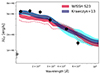 |
Fig. 1. SED fitting results for J083+11.8 at z = 6.346 using lum-K13 (blue) and WISSH-S23 (red) templates. The thickness of the lines denotes the ±1σ interval. Gray points denote photometry below the Lyα. The cyan shaded area and the dashed red lines denote the ±1σSED region associated to the best fit for the lum-K13 and WISSH samples, respectively; see Sect. 3.1. |
The HYPERION QSO SEDs with the final best fits for both lum-K13 and WISSH-S23 templates are reported in Fig. 2, while the figures showing the modeling with lum-K13 for the E-XQR-30 sample are available on Zenodo. Upon visually inspecting the fitted SEDs, we observe that the data points with λ < 1 μm are generally well fitted, while those at longer wavelengths exhibit larger discrepancies from the model (see also Sect. 7). This outcome is expected: as previously discussed, QSOs tend to show greater scatter around their mean value in the NIR region.
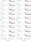 |
Fig. 2. Results of the SED fitting of the HYPERION QSOs using the lum-K13 (blue) and S23 (red) templates. The dotted blue and dashed red lines give the unextincted SEDs, which have been extended below the Lyα with a double power law as explained in Sect. 3.3; Lbol is the integral under the dotted/dashed lines. Data at UV wavelengths shorter than Lyα were not considered in the fitting and are colored gray. The cyan stars indicate measured 1 keV luminosities; see Table 3. The subpanels show the residuals with respect to the K13 best-fit SED. The black circles refer to the residuals computed using only the uncertainties on the photometric points, while the red crosses represent residuals for which also the scatter on the SED template was taken into account. |
Two notable exceptions with particularly poor fits in the UV–optical region –although their  are not the worst– are PSOJ023−02 and SDSSJ0836+0054. PSOJ023−02 has a very flat SED, which is not well modeled by reddening and may be intrinsic in nature, as it does not display the typical curling of the SED caused by dust extinction (i.e., the reddening is stronger at shorter wavelengths; see Hopkins et al. 2004). In contrast, the fit for SDSSJ0836+0054 is quite accurate for most points, except for the SpitzerS4.5 data point, which is significantly more luminous than the modeled SED. While we cannot definitively explain this discrepancy, a plausible reason could be that the S4.5 flux is overestimated. This is supported by the fact that, although probing almost the same wavelength range, the value reported for the W2 filter is 0.28 mag fainter.
3.3. X-ray and EUV SED modeling
To model the SEDs in the unobserved extreme UV (EUV; 12.4 ≤ λ/Å < 1216), we followed the method discussed in Lusso et al. (2012) and Shen et al. (2020), who use a power-law with a fixed slope of λLλ ∝ λ0.8 in the range between 500 ≤ λ/Å ≤ 1216, which was derived from HST observations of local AGN (Zheng et al. 1997; Telfer et al. 2002; Lusso et al. 2015), plus a power law with a free-to-vary spectral slope α that links L500 Å with the 1 keV luminosity. Thus, the full SED template takes the following form:
 (3)
(3)
The derived α for HYPERION QSOs are reported in Table 2. The same is valid for the E-XQR-30 QSOs but, as there are no 1 keV luminosities, we employed the value obtained as the geometric mean of the HYPERION sample, which is Log(λL1 kev) = 45.01 ± 0.08 erg/s. The advantage of using a double power law to describe EUV emission lies in the fact that it allows us to make use of both the information available on the QSOs emission just below the Lyα line (from low-z sources) and the high-quality X-ray data obtained for these sources at z ≥ 6. This would not have been possible if using a fixed template or extrapolating with a single power law.
Spectral slopes of the HYPERION QSOs.
As the EUV contributes nearly 50% of the QSO emission, different modelings could lead to significantly different derived Lbol, which is the main value we want to derive. Therefore, we tested the impact of different modelings on the integrated luminosity under the EUV region. Our double-power-law parametrization yields, on average, EUV luminosities that are ∼20% larger than those derived using the EUV modeling of lum-K13, with differences of up to 40%. Conversely, employing a single-power-law extrapolation yields an average decrease of 8%, with a maximum deviation of 38%. Finally, by employing the far redder EUV spectral slope recently proposed by Cai & Wang (2023), we obtain EUV luminosities that are 70% lower than those obtained when using the double-power-law parametrization. Figure 3 shows these three different modelings for the case of J036+03.0, which, in terms of optical-to-X-ray ratio, can be considered as representative of the entire HYPERION sample (see Zappacosta et al. 2023).
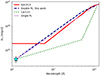 |
Fig. 3. Different parametrizations considered for the EUV modeling of the SEDs applied to J036.5+03.0; see Sect. 3.3. |
We also tried to quantify the possible uncertainties associated with the fact that we assumed an average L1 keV calculated from the HYPERION sample for E-XQR-30 sources. Indeed, although the proper X-ray emission –that is, ∼ 20 Å−1 keV– only accounts for less than 1% of Lbol in these luminous QSOs (e.g., Duras et al. 2020), the 1 keV luminosity constrains the slope of the second power law in our modeling of the unseen EUV SED, and thus may potentially affect Lbol. To quantify the impact of this assumption, we simulated a QSO with log(L2500 Å) = 47 erg/s and we calculated how much Lbol varies in the case where it has an X-ray luminosity of twice (half of) that predicted by the relation by Lusso et al. (2010), finding an increase (decrease) in Lbol of ∼4%.
4. Bolometric luminosities, E[B − V], and bolometric corrections
The bolometric luminosities for the HYPERION and E-XQR-30 QSOs were computed by integrating their dereddened SEDs obtained using the lum-K13 template between 1 keV and 1 μm, where the choice of integration limits ensures that reprocessed radiation is not included and thus that the same contribution is not counted twice (see Marconi et al. 2004). Assuming that Lbol were computed without dereddening the SED, we would obtain lower values for Lbol, with a difference of Δlog(Lbol)≈4 × E[B − V], which is nearly linear within the range of E[B − V] explored by our sources. Lbol values are provided in Table 3 (HYPERION sources) and on Zenodo (E-XQR-30 sources), together with monochromatic luminosities at various wavelengths obtained by interpolating two adjacent photometric points and correcting for the SED-fitting-derived E[B − V] of the source. We also calculated λEdd assuming the MSMBH derived from the MgII line, single-epoch virial-mass estimator (see Table 1 and Zappacosta et al. 2023; Mazzucchelli et al. 2023, for further references and for the associated uncertainties).
Bolometric and monochromatic luminosities of the HYPERION QSOs.
In Fig. 4, we show the luminosity distributions of both the HYPERION and E-XQR-30 samples, which range within 46.5 ≲ log(Lbol/[erg/s]) ≲ 48.1; performing a Kolmogorov-Smirnov test on the Lbol distributions of the two samples gives a p-value of ∼0.05 (i.e., it does not reject the hypothesis that both samples have been drawn from the same distribution), thus strengthening our choice of using the E-XQR-30 QSOs as a complementary sample to HYPERION.
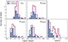 |
Fig. 4. Bolometric and monochromatic luminosities and E[B − V] distributions for the HYPERION (blue) and E-XQR-30 (purple) samples. |
In Fig. 5 we compare Lbol with those computed via BC and LBC (Mazzucchelli et al. 2023; Zappacosta et al. 2023, and references therein). We find that, when integrating the full SED, we obtain systematically lower values with ⟨Δ(Lbol)⟩ = 0.13 ± 0.08 dex on average (i.e., LBC are overestimated by 34%) and discrepancies of up to ∼0.25 dex in a few QSOs. However, we note that LBC were derived using the 3000 Å bolometric correction BC3000 Å = 5.15 (Richards et al. 2006; Shen et al. 2011), which is obtained by integrating the entire SED between 10 keV and 100 μm. Therefore, including also X-ray and IR reprocessed emission leads to overestimation of Lbol when compared to our values. This overestimation also impacts the determination of λEdd, which we find to be 0.12 ± 0.06 dex lower than the previous measurement on average.
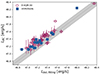 |
Fig. 5. Lbol already published (Zappacosta et al. 2023; Mazzucchelli et al. 2023) vs Lbol computed in this work. Lbol has been computed in the literature using the 3000 Å BC (Lbol = 15.5 L3000 Å). The black line gives the 1:1 ratio, while the gray shaded area delimits the 0.1 dex difference region. |
Regarding the derived E[B − V], the distribution is dominated by sources not affected by dust reddening, that is, with E[B − V] = 0; see the right panel of Fig. 4. However, we notice a slight disagreement between the HYPERION and E-XQR-30 samples; while only J0224−4711 among the HYPERION QSOs has E[B − V]≥0.05, there are 11 E-XQR-30 sources with E[B − V] values exceeding this value (excluding J0224−4711). Given the relation between dust extinction and the presence of BAL features (Gallagher et al. 2007; Bischetti et al. 2022), this difference can be accounted for by the fact that, while broad absorption lines are found in 47% of E-XQR-30 sources, only J0038−1527 (Wang et al. 2018) and J231−20 (Bischetti et al. 2022) have published BAL features among HYPERION QSOs (although, to date, no BAL feature analysis has been performed as systematically and consistently as that carried out for the E-XQR-30 QSOs). A potential caveat regarding the correlation between BAL troughs and increased dust extinction is that QSOs may appear reddened not due to genuine reddening but because their intrinsic fluxes are underestimated in regions of the spectrum affected by absorption features. However, while this could indeed be true for low measured E[B − V] values (∼0.01 − 0.03), the absorption features typically observed in the E-XQR-30 sample are not deep enough to influence flux measurements to the extent that they could mimic the effects of significant E[B − V]. Moreover, Bischetti et al. (2022) already noted that BAL QSOs in the E-XQR-30 sample exhibit redder W1 − W2 colors, which are bands that do not probe wavelengths affected by absorption troughs.
As mentioned, the measurement of Lbol for high-z QSOs usually relies on the application of a bolometric correction, especially the 3000 Å one. As the values we used were derived from lower-z sources, we investigated whether these values are appropriate for objects at the EoR or it is necessary to use different values. In the left panel of Fig. 6, we show our derived BC3000 Å for the HYPERION and E-XQR-30 QSOs compared to the constant bolometric correction by Richards et al. (2006), of namely BC3000 Å = 5.15, which has been adopted in the literature as a standard BC3000 Å for z > 6 QSOs (e.g., Wu et al. 2015; Bañados et al. 2018; Reed et al. 2019; Shen et al. 2019; Yang et al. 2021; Farina et al. 2022; Mazzucchelli et al. 2023; Fan et al. 2023; Zappacosta et al. 2023). We also show a re-evaluation of this value by Runnoe et al. (2012), of namely BC3000 Å = 3.11, who exclude reprocessed IR emission, which allows a fair comparison with our value. The BC3000 Å distribution of HYPERION and E-XQR-30 sources ranges between 2.64 and 3.94, with a mean value of 3.30 ± 0.3. The majority of derived BCs are higher than the recalculated BC3000 Å by Runnoe et al. (2012), although they are still in full agreement within the uncertainties. This small discrepancy, rather than arising from a different SED shape in our objects, can be attributed to our more careful modeling of the EUV (i.e., with the double power law) which, as mentioned above, results in higher Lbol (and consequently higher BC) than those obtained using an average SED template. The right panel of Fig. 6 illustrates that when computing Lbol with the lum-K13 EUV recipe, the BCs are fully consistent with the predictions by Runnoe et al. (2012).
 |
Fig. 6. BC3000 Å vs Lbol for HYPERION and E-XQR-30 QSOs with their weighted mean value reported as a dark-blue square. The left panel illustrates Lbol computation using Eq. (3), while the right panel showcases results obtained through the lum-K13 modeling of the EUV. The constant 3000 Å BCs proposed by Richards et al. (2006) are overplotted. The original value of 5.15 is depicted as a black dot-dashed line while, the version recomputed by Runnoe et al. (2012) to exclude IR emission is represented as a red solid line. |
Given our more refined treatment of the UV-X-ray SED, which gives more accurate Lbol measurements, we recommend using the revised BC3000 Å value instead of 5.15 to recover a more accurate Lbol for z > 6 QSOs. This allows the removal of a further source of inaccuracy in the determination of λEdd, which is already affected by systematic uncertainties from the mass determination.
Additionally, we computed optical bolometric corrections at 4400 Å and 5100 Å, comparing them to relationships established for lower-z sources, as depicted in Fig. 7. For λ = 4400 Å, the bolometric corrections demonstrate a good agreement with the average value reported in Duras et al. (2020) for a large collection of AGN at 0 ≲ z ≲ 3, resulting in a mean of 4.9 ± 0.7. In the case of 5100 Å BC, our derived BC5100 Å values are consistent with the predictions at higher luminosities extrapolated from the relationship provided by Runnoe et al. (2012). However, they almost all exceed the value reported in Krawczyk et al. (2013), although our mean value of BC5100 Å = 5.7 ± 0.9 remains in agreement within 2σ with that of these latter authors.
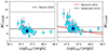 |
Fig. 7. Bolometric corrections at 4400 (left) and 5100 Å (right) with their weighted mean values reported as blue squares. Overplotted are the relationships by Duras et al. (2020), Krawczyk et al. (2013, with the associated uncertainties as dotted lines), and Runnoe et al. (2012). |
5. Predicting X-ray luminosity with a physically motivated AD model
We made use of QSOSED (Kubota & Done 2018), a physically motivated model for disk and corona emission, to describe the nuclear emission of QSOs. Specifically, we aimed to determine whether or not these models can accurately predict the coronal emission (i.e., the 1 keV luminosities) by fitting only the accretion disk data, which include the rest-frame UV and optical photometric points. Accordingly, our analysis is limited to the 18 HYPERION QSOs. QSOSED assumes that the emitted radiation originates from three distinct regions at increasing radial distances: (i) a hot (kB T ≳ 10 keV) comptonizing plasma (i.e., the corona; e.g., Haardt & Maraschi 1991) at RISCO < r ≤ Rhot, which is responsible for the power-law-like X-ray continuum emission, (ii) a warm (kB T ≲ 5 − 10 keV) comptonizing plasma in an intermediate region, Rhot < r ≤ Rwarm, which contributes to the soft excess (Petrucci et al. 2018), and (iii) a standard, geometrically thin, optically thick accretion disk at r > Rwarm. Furthermore, QSOSED assumes that the hot corona radiates 2% of the Eddington luminosity of a source, regardless of its Lbol.
SED templates calculated by QSOSED were generated through the X-ray spectral fitting program XSPEC (Arnaud 1996) by taking into account four main free parameters, namely MSMBH, the BH spin, the specific mass-accretion rate, ṁ, and the cosine of the inclination angle i, cos(i). Given the high probability of resulting in degenerate templates given the relatively low number of degrees of freedom (i.e., photometric points), we fixed the BH spin to zero, MSMBH to the values listed in Zappacosta et al. (2023), and the viewing angle to 30°, which is an average value among those expected for type-1 QSOs (e.g., Mountrichas et al. 2021). Accordingly, the only parameter left free to vary is log(ṁ), which ranges from −1 to 0.4 in steps of 0.1. Furthermore, we did not account for dust reddening as we derived it from the empirical modeling, finding it to be negligible for the vast majority of the sources (see Table 3). In QSOSED, the luminosity from the QSOs and thus the observed flux at each wavelength are predetermined without any normalization. Given the many assumptions on our input parameters, and the systematic uncertainties on MSMBH, (∼0.55 dex; e.g., Mazzucchelli et al. 2023), we expect a limited accuracy in the SED description, which, we emphasize, is not the main result we aim to achieve with this analysis. In this model, we cannot continuously explore the parameter space, as the allowed values of ṁ are discretized. Thus, the best fit was determined via  minimization, while uncertainties were estimated by identifying the range of ṁ that resulted in
  from the best fit, corresponding to a 1σ confidence interval (e.g., Avni 1976).
The results from the fits, shown in Fig. 8 together with the derived ṁ, indeed reveal a relatively large range of  values, varying from 1.4 for J1120+0641 to ∼20, with J029−26 being a notable outlier with
  and a
and a  median value of 7.2. Interestingly, among the 13 QSOs for which the QSOSED template provides an acceptable fit (arbitrarily chosen to be those with
  ), the 1 keV fluxes predicted by QSOSED are consistent with the measured ones within 3σ for 7 sources (54%) and within 5σ for 9 sources (70%). By examining the difference in the ratio of predicted to measured fluxes, QSOSED models deviate by a median factor of 1.6, with a maximum discrepancy factor of 6.3 in the case of J083+11.8. This outcome highlights the effectiveness of QSOSED in predicting X-ray emission based solely on the observed luminosity from the accretion disk even in the case of the most distant QSOs. We note that, for the three sources showing a significant difference between observed and QSOSED predicted X-ray fluxes (namely, J0411−0907, J083+11.8, and J0050+2445), the observed X-ray flux is always lower than the predicted one by factors of 2.7, 6.3, and 3.8, respectively.
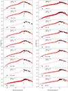 |
Fig. 8. Same as Fig. 2 but with QSOSED generated templates. Each panel presents the mass accretion and the |

The deviation of the QSOSED prediction at 1 keV from the actual data may reflect either (i) the deviations from intrinsic physical properties (e.g., mass measurement, spin assumption, source inclination, and lack of extinction) for some sources or (ii) the underlying assumptions on which this model is based, such as the fraction of the X-ray coronal emission in terms of LEdd, and Rhot and Rwarm, the temperature of the hot and warm Comptonizing regions. An investigation into the cause of the disagreement is beyond the aim of this paper and is deferred to future work.
Finally, in light of the good predictive results demonstrated by QSOSED, we performed the fitting on E-XQR-30 QSOs, taking into account the same assumptions (i.e., i = 30°, spin = 0), in order to estimate their 1 keV fluxes, which are reported, converted to luminosities, on Zenodo, along with the other derived properties.
6. Ultraviolet and optical slopes
The optical–UV SED is usually modeled as a broken power law, with the break between the two slopes falling at λ = 3000 − 5000 Å (e.g., Vanden Berk et al. 2001; Temple et al. 2021a). To derive the slopes of the HYPERION and E-XQR-30 QSOs, we opted to follow Lusso & Risaliti (2016), that is, we set the break at λ = 3000 Å; although we extended the UV interval down to 1300 Å instead of 1450 Å in order to include the Y band photometric point for a greater number of QSOs, without being affected by the peak of the Lyα emission. Therefore, we refer to βUV as the UV slope, characterizing the accretion disk emission between λ = 1300 Å and 3000 Å, and γopt as the optical slope, describing the emission at longer wavelengths, up to λ = 1.0 μm, where the SED shows an inflection due to the arising contribution from hot dust. Spectral slopes are reported in luminosity density units, that is, in the form Lν ∝ νβ.
Slopes were computed independently via least-square minimization by fitting a straight line to the photometric points in the log-log space. To compute the slope, we required the QSOs to have at least three photometric points in the wavelength interval of interest; this requirement limits the number of QSOs with measured βUV and γopt to 39 and 30, respectively. In particular, all but three sources with computed γopt belong to the E-XQR-30 sample, as they have lower redshifts (indeed at z ≳ 6.3, the K band moves to shorter wavelengths than 3000 Å). Figure 9 shows the computed βUV and γopt distribution (reported in Table 2 for HYPERION QSOs and on Zenodo for E-XQR-30 ones). For comparison, we also show the contour enclosing the 39th and 86.4th percentiles (respectively 1 and 2σ under the assumption of a bivariate normal distribution) of the values derived from the Krawczyk et al. (2013) luminous subsample following an analogous methodology. Additionally, as the derived slope could vary as a function of z simply because the filters are sampling different regions of the SED, we also overplot the mean ±1σ values obtained by redshifting the lum-K13 template at 5.5 ≥ z ≥ 7.5 and generating mock observations with UKIDSS YJHK plus W1 and W2 filters for different levels of E[B − V].
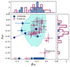 |
Fig. 9. βUV (1300 < λ/Å < 3000) and γopt (3000 < λ/Å < 10 000) distributions for the sample. Only the UV slope has been measured for the points along the constant line γopt = −1.5. Blue stars represent the values obtained from the lum-K13 template assuming E[B − V] values of 0, 0.05, and 0.1, and assuming observations in the UKIDSS YJHK bands plus W1 and W2 for QSOs at 5.5 ≥ z ≥ 7.5. The shaded light-blue areas delimit the 1 and 2σ confidence intervals for the luminous QSO subsample in Krawczyk et al. (2013). |
The HYPERION and E-XQR-30 sources are in complete agreement with the ranges of values observed in luminous QSOs at lower z, and, considering the uncertainties –which are quite large due to the fact that the fitting is performed on a limited number of points–, the bulk of the sample agrees with the point obtained from the lum-K13 template without dust extinction. QSOs with a lower βUV (i.e., a flatter SED) can be explained through dust reddening and indeed they are generally those with higher E[B − V] values. In particular, the three HYPERION sources with lower βUV are those with measured E[B − V] ≥ 0.03 (see Table 3). Conversely, two E-XQR-30 QSOs exhibit bluer βUV than the rest of the population, although still within ∼2σ of the distribution observed in Krawczyk et al. (2013), while PSOJ023−02, located in the bottom-right corner of Fig. 9, shows a γopt value that is in significant disagreement with the rest of the distribution. As already mentioned in Sect. 3.1, this object has a rather flat spectrum and hence the low γopt is expected. Finally, we tested for potential correlations between βUV and both the photon index Γ and the UV-to-X-ray ratio αOX, defined as −0.384 log(Lν,2keV/LLν,2500ÅÅ) and reported in Zappacosta et al. (2023) and Tortosa et al. (2024). However, we find no evidence of correlation among these parameters. Indeed we simulated multiple realizations of the datasets by generating synthetic values normally distributed around the best-fit value and with a σ equal to their uncertainties and, performing Spearman tests for each of them, obtained mean correlation coefficients and p-values of 0.22 and 0.4 for the Γ versus βUV relation and −0.05 and 0.6 for αOX versus βUV.
7. Near-infrared modeling of the hot-dust component
It is intriguing to compare the positions of MIR points (Spitzer MIPS 24 μm, W3, and W4) to what is expected from the normalized SED templates. Previous studies (e.g., Jiang et al. 2006; Leipski et al. 2014; Bosman et al. 2024) reported a NIR emission of QSOs at the EoR resembling that of luminous objects at lower z, characterized by a black-body-like continuum originating from a hot-dust component close to its sublimation temperature. However, there are several indications suggesting a higher fraction of dust-poor objects at the EoR, with a lower-than-average NIR-to-optical emission ratio (Jiang et al. 2006; Leipski et al. 2014) or even dust-free sources (Jiang et al. 2010). In these cases, the NIR can be well-modeled by assuming only emission from the accretion disk, which is modeled as a power law, without the need to add emission from hot dust. The cause of the observed lack of dust in these QSOs remains uncertain. It could be attributed to a genuine deficiency of dust, possibly linked to these sources being in the early stages of the Universe (Jiang et al. 2010). Alternatively, it may be associated with a distinct torus structure, characterized by a lower covering factor, resulting in less dust being directly exposed to the primary radiation (see Lyu et al. 2017).
In total, we have 11 QSOs where the 24 μm or the W4 photometry is available, which is necessary to constrain the hot dust emission. We find that in 4 of these, the lum-K13 SED agrees with the true NIR luminosity, while 5 objects have enhanced NIR emission and 2 objects have substantially lower emission.
To better quantify the strength of the hot-dust emission, following the approach by Temple et al. (2021b), we computed XHD = LBB/LAD for our sources, which is the ratio at λ = 2 μm between the hot-dust and accretion disk components. More specifically, we modeled the QSO SEDs at λ > 3000 Å with a power law describing the emission from the accretion disk plus a single-temperature black-body, which represents the emission from hot dust located in the innermost layer of the torus, that is,
Following Temple et al. (2021b), we fixed both the temperature of the black body (T = 1280 K) and the slope of the power law (γopt = −0.16). We kept T fixed, as the only point useful to constrain the black-body emission is the Spitzer 24 μm one (or, alternatively, W4), while we fixed γopt to compare our results against those by Temple et al. (2021b), who showed that the derived XHD values strongly depend on the assumed γopt. However, we note that the assumed slope is remarkably close to the one we obtain in Sect. 8 for the mean SED and can therefore be considered as an average value; although it is slightly different from the mean of the individual γopt computed in Sect. 6, which is ⟨γopt⟩= − 0.23. In addition, by visually inspecting the fitting results, we find that the optical emission of the 11 analyzed sources is generally well described by this power law. As done for the SED fittig routine, the constants of normalization K1 and K2 were derived by minimizing the likelihood.
The results of the fitting are shown in Fig. 10. For each of the analyzed QSOs, it is necessary to add a hot-dust component, and therefore there are no QSOs without a dust component in our sample. We find the median value of XHD to be 2.4, with a MAD of 1.4, which is in agreement with the 2.5 median value reported in Temple et al. (2021b); moreover, a K-S test (p-value = 0.19) indicates no evidence of a different underlying XHD distribution compared to that derived by Temple et al. (2021b).
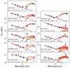 |
Fig. 10. NIR SEDs for the 11 QSOs with MIR photometry. The blue line gives the accretion disk emission modeled as a power law with a spectral index of −0.16, while the gold line describes the emission from hot dust modeled as a black body with T = 1280 K. The red lines show the sum of the two components. |
Specifically, two sources, namely J0100+2802 and SDSSJ0836+0054, exhibit XHD ≤ 1. While only J0100+2802 can be considered –within 1σ– as properly dust poor according to the criterion set by Jun & Im (2013), which requires XHD ≤ 0.15 (see Temple et al. 2021b), both sources clearly show much lower dust emission than expected. Notably, SDSSJ0836+005 was previously identified as a QSO with dust deficiency by Leipski et al. (2014). On the other hand, three QSOs, ULASJ0148+0600, SDSSJ0842+1218 and SDSSJ0927+20, are found to have XHD ≥ 4.7.
Temple et al. (2021b) reported a positive correlation between XHD and the velocity of the CIV emission line relative to the systemic MgII-derived redshift (hereafter, CIV blueshifts), suggesting objects with faster winds have stronger hot-dust emission. Figure 11 shows the addition of the 11 HYPERION and E-XQR-30 sources to the original plot of these latter authors. Our sources do not show any clear CIV-XHD correlation. However, this result is primarily due to two factors. First, the very small sample size poses challenges in determining the correlation. As a test, we randomly selected 11 sources from the data presented in Temple et al. (2021b), and only in 25% of the cases did we recover a positive correlation with a p-value < 0.05. Second, and more importantly, our sources exhibit significantly faster winds compared to the QSOs in Temple et al. (2021b), as expected for such luminous sources (Fiore et al. 2017; Vietri et al. 2018; Meyer et al. 2019; Timlin et al. 2020; Schindler et al. 2020). Consequently, a majority of our objects lie outside the contour enclosing 86.4% (i.e., 2σ) of the Temple et al. (2021b) QSOs.
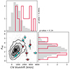 |
Fig. 11. XHD vs CIV blueshift adapted from Fig. 3 in Temple et al. (2021b) with the inclusion of HYPERION and XQR-30 QSOs. E-XQR-30 blueshifts are taken from Mazzucchelli et al. (2023), while HYPERION values are computed as the mean of all the blueshifts reported in the literature for each QSO; see Tortosa et al. (2024). Errors on XHD are given as the 16th and 84th percentiles. Cyan stars indicate QSOs with Spitzer MIPS 24 μm fluxes, while red stars have W4 photometry. The histograms show the distributions of CIV blueshift and XHD in Temple et al. (2021b, shown here in gray, and normalized by a factor of 500) and for the HYPERION and E-XQR-30 QSOs (red). The p-values obtained by performing a K-S test on the two distributions are reported next to the histograms. |
8. The mean spectral energy distribution of luminous, z > 6 QSOs
We generated a mean SED based on the combined HYPERION and E-XQR-30 samples to obtain a more comprehensive view of the broadband emission of luminous high-redshift QSOs. As our sample consists of QSOs with a relatively narrow redshift range, each observed band probes similar rest-frame wavelengths across all QSOs. Therefore, instead of constructing a continuous SED template, we determined the mean luminosity value for each band. With this approach, we do not need to extrapolate the SED to wavelengths not covered by certain QSOs. We also grouped Spitzer IRAC 3.6 and W1, Spitzer IRAC 4.5 and W2, Spitzer MIPS 24 and W4 as the same band; the J1120+0641 1 μm luminosity point was included with Spitzer MIPS 8 μm. To minimize the scatter due to the small sample size of our analyzed QSOs, we normalized their SEDs at 3500 Å. The normalization is particularly relevant for the W3 and W4 bands, where most sources in our sample have not been detected. Indeed, as brighter QSOs are more likely to be detected, using non-normalized data would result in a mean NIR emission that is not representative of the true mean properties of the sources. Although there is no physical reason to choose a specific normalization wavelength, we tested various wavelengths within the range of 2000 Å < λ < 7000 Å and found that normalizing at 3500 Å resulted in the lowest scatter across all bands. Therefore, we adopted this wavelength as our normalization point.
Figure 12 shows the resulting mean SED, with the uncertainties given as the standard deviation divided by the square root of the number of QSOs in each band, along with a comparison with the mean SEDs derived in Krawczyk et al. (2013) for both their luminous and whole QSO sample (dot-dashed blue line and dotted purple line, respectively) and WISSH-S23 (dashed green line).
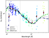 |
Fig. 12. Photometry points for the HYPERION and E-XQR-30 samples, normalized at λ = 3500 Å. The red diamonds show the geometric mean value for each band with the associated 1σ as an error bar. Overplotted are also the mean SEDs by Krawczyk et al. (2013) (whole and luminous QSOs samples, purple dotted and blue dot-dashed lines, respectively) and the WISSH hyperluminous mean SED (dashed green line). The vertical dotted lines indicate the position of the Lyα at 1216 Å and the normalization wavelength. |
As visible in Fig. 12, we do not find any significant deviations from the mean SEDs of luminous QSOs at lower z (i.e., lum-K13 and WISSH-S23), while the average SED by Krawczyk et al. (2013), labeled “all-K13”, has a flatter UV-optical slope and, depending on the chosen normalization wavelength, predicts larger emission at λ ∼ 6000 − 9000 Å as in Fig. 12, or a lower UV bump. Therefore, we do not find any evolution of the SED with redshift, at least for the 1000 Å–1 μm wavelength interval. While there might be a selection effect, given that all our sources were identified by targeting objects with typical colors of lower-z QSOs (e.g., Reed et al. 2019), and therefore may not be universally applicable to the entire population of high-z AGN, this result strengthens our choice to employ templates of luminous QSOs for computing bolometric luminosities.
At wavelengths above 1 μm, the distribution of rest-frame NIR points shows a considerable spread; there is an indication of even stronger NIR emission than in the IR-selected WISSH QSOs, although this needs to be further investigated, as the currently limited data do not allow robust conclusions to be made. Moreover, the W3 and W4 points are likely biased toward NIR-bright sources, as the limiting magnitudes in these bands are much shallower than those of W1 and W2.
We fitted the mean SED with a broken power law jointed at λ = 3000 Å, plus a blackbody with a fixed temperature of T = 1280 K, as described in Sect. 7. For all parameters, we assumed flat priors. We find βUV = −0.63 ± 0.05, which is in agreement with both the value reported in Telfer et al. (2002, i.e., −0.69, from the analysis of 184 QSOs with HST spectra) and that presented by Lusso et al. (2015, i.e., −0.61, derived from 53 luminous sources at redshift z ∼ 2.4). This value of βUV is instead softer than both what is found in the composite spectrum by Selsing et al. (2016) derived from 102 QSOs at z = 1−2.1 and also that found by Temple et al. (2021a) from a subsample of bright SDSS QSOs (18.6 < i < 19.1), that is, βUV = −0.30 and −0.349, respectively. The power law modeling the mean SED redwards of 3000 Å is found to be steeper with a slope of γopt = −0.14 ± 0.04. Interpreting γ as the mean optical slope, we confirm that high-luminosity QSOs have a steeper optical continuum (e.g., Richards et al. 2006; Krawczyk et al. 2013) even at high redshift with respect to the bulk of the population at lower luminosities (i.e., γopt = −0.46; Vanden Berk et al. 2001). Interestingly, computing the hot dust-to-AD ratio with this modeling gives XHD = 3.28 ± 0.5, which is higher than both the median value found by Temple et al. (2021b) and that calculated as the mean of the individual QSOs.
The continuous SED template obtained by the broken power-law plus black-body modeling is shown in Fig. 13. To connect the template with the mean 1 kev luminosity, we extended the SED in the EUV region using the same recipe as that reported in Eq. (3).
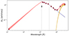 |
Fig. 13. Continuous mean SED obtained by fitting the mean points (red diamonds) with a broken power law (λbreak = 3000 Å) plus a single temperature (T = 1280 K) black body. The EUV SED (λ < 1216 Å) was reconstructed as discussed in Sect. 3.1. The light blue and gold shaded area describe the best-fit broken power law and black body, respectively. The gray diamond was excluded from the fit as it is also the average of points falling below the Lyα. The black dotted lines indicate the Lyα and the normalization wavelength at 3500 Å. |
We also computed the mean SEDs of several subsamples obtained by splitting the sample based on the median of several physical properties (MSMBH, CIV blueshift, Lbol) or on the criterion adopted to assemble the HYPERION sample (i.e., using Ms, Edd = 1000 M⊙ as threshold) but found no significant difference either between them or with respect to the overall average SED (see Fig. 14). This result holds true even when comparing the mean values of βUV and γopt of each subsample, as shown in Fig. 15. Indeed, each pair of values is in agreement with that of its complementary subsample within 2σ.
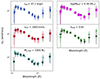 |
Fig. 14. Mean SEDs derived by splitting the sample according to the median value of several physical properties. Each panel reports the threshold value used to split the sample. Filled markers refer to QSOs above the threshold, while empty ones indicate QSOs below the threshold. |
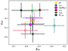 |
Fig. 15. Mean γopt vs mean βUV computed for each subsample. Errors are reported as the standard deviation of the values divided by the square root of the number of sources in the subsample. The yellow triangle shows the mean value for the full sample. As in Fig. 14, filled markers refer the subsample above the threshold, while empty ones refer to the one below. |
9. Summary and conclusions
In this work, we characterize the X-ray-to-NIR broad-band emission of luminous QSOs at the EoR with the main goal being to provide the first systematic investigation of the SED of these sources. Our main results can be summarized as follows:
-
We produced X-ray-to-NIR SEDs for the 18 QSOs belonging to the HYPERION sample (Zappacosta et al. 2023; Tortosa et al. 2024). Exploiting the unprecedented quality of X-ray data from the HYPERION QSOs, we employed a double power law to characterize the X-ray to UV SED (Lusso et al. 2012, see Eq. 3); given the absence of data in that wavelength range, this modeling ensures the most reliable representation of the EUV region achievable at present. The UV-to-NIR SED of the QSOs was instead modeled using templates derived from luminous QSOs at lower z, namely lum-K13 (Krawczyk et al. 2013) and WISSH-S23 (Saccheo et al. 2023). We find that, for all QSOs, the optical–UV region is well described by the lum-K13 SED (see Fig. 2), while we obtained, on average, poorer results when employing the WISSH-S23 SED; although these latter span a luminosity range closer to the HYPERION sources.
-
We increase the statistical significance of our analysis in the UV-to-NIR region by including an additional 36 QSOs drawn from the E-XQR-30 sample (D’Odorico et al. 2023), which share similar properties with HYPERION sources in terms of redshift and luminosity. We confirm that the lum-K13 template also provides excellent results in describing the SED of these sources.
-
By integrating the SEDs, we homogeneously computed bolometric luminosities for all 54 objects. Their values range from 46.8 ≤ log(Lbol)≤48.1, as shown in Fig. 4. We find that our derived Lbol are systematically lower than the ones already reported in the literature, with an average discrepancy factor of 0.13 dex.
-
We calculated bolometric corrections at 3000, 4400, and 5100 Å for QSOs with redshifts of z ≥ 5.5 and check their consistency with those derived from lower z sources. Given the similarity of the SEDs of our QSOs to those of their lower z counterparts, the obtained bolometric corrections are broadly consistent with literature findings. However, we observe that the values for λ = 3000 Å and 5100 Å are systematically larger than the bolometric correction values largely used in the literature. As an improved estimate for these sources, we show that better results are obtained when using BC3000 Å = 3.3 and BC5100ÅÅ = 5.7 to derive Lbol.
-
Taking advantage of the X-ray coverage of HYPERION, we verified the accuracy of theoretical models (Kubota & Done 2018) in predicting coronal emission from that of the accretion disk for these high-z sources. Despite the many crude assumptions we make regarding the parameters, we surprisingly find that models and observations deviate by a median factor of just 1.6.
-
We investigated the hot-dust emission in 11 QSOs with available MIR data by modeling their rest-frame NIR using a combination of a power law and a black body (see Sect. 7 and Fig. 10). Our analysis reveals that, for all these sources, the inclusion of a dust component is necessary, although to a varying extent. We quantified the hot-dust emission strength by computing the hot-dust to accretion-disk emission ratio XHD (Temple et al. 2021b). The overall XHD distribution is consistent with that found by Temple et al. (2021b, cf. our Fig. 11), but two QSOs exhibit a notably low XHD, with one source, J0100+2802, being within 1σ of the threshold outlined in Jun & Im (2013) for classification as dust poor. On the other hand, three sources have a XHD that is approximately twice the average value observed in luminous QSOs.
-
Finally, we derived a mean SED for these high-z QSOs extending from the X-ray to NIR (i.e., from 1 keV to about 3 μm); see Figs. 12 and 13. This average SED is in excellent agreement with the mean SEDs of luminous QSOs, demonstrating that, for the analyzed sample, we do not find any redshift evolution of the shape of the SED, at least in the optical-UV region. As typically reported for luminous QSOs at lower-z, we find that optical emission at 3000 Å < λ < 1 μm is well described by a power law with a steeper slope (Fν ∝ ν−0.14) than observed in the bulk of the low-luminosity AGN population; that is, Fν ∝ ν−0.46 (Vanden Berk et al. 2001).
As a natural extension of this work, we aim to (i) increase the sample size of QSOs at z > 6 − 7 with good X-ray data and (ii) include rest-frame photometric points at λ > 1 μm thanks to JWST/MIRI observations in order to obtain a uniform NIR coverage. Improving these aspects will be fundamental for highlighting potential redshift-dependent properties, which we have so far been unable to constrain in a significant way. To this end, a recently accepted XMM-Newton Large Program (PI Zappacosta) will allow the investigation of X-ray emission also in sources with low Ms, Edd. In the NIR, it will instead be critical to increase the number of sources with photometric coverage to confirm the tentative indication from the computed mean SED that, on average, EoR sources exhibit enhanced emission from hot dust compared to average templates. JWST/MIRI observations will play a crucial role in adequately sampling the SED in the 1 to 2.5 μm region, providing a systematic characterization of hot-dust emission in these early quasars.
Data availability
All the photometric data used in this work are available on Zenodo at https://zenodo.org/records/14181275. The same repository also contains the derived bolometric and monochromatic luminosities, as well as the spectral slopes, for both the HYPERION and E-XQR-30 samples.
Acknowledgments
We are grateful to the anonymous referee for their useful comments and suggestions which helped us to improve the paper. The authors acknowledge financial support from the Bando Ricerca Fondamentale INAF 2022 Large Grant “Toward an holistic view of the Titans: multi-band observations of z > 6 QSOs powered by greedy supermassive black holes”. AB, MB, MB, SC, VD, FF, CF, SG, VT, NM, LZ acknowledge support from the European Union – Next Generation EU, PRIN/MUR 2022 2022TKPB2P – BIG-z. MB acknowledges support from INAF project 1.05.12.04.01 – MINI-GRANTS di RSN1 “Mini-feedback” and from UniTs under FVG LR 2/2011 project D55-microgrants23 “Hyper-gal”. DD acknowledges PON R&I 2021, CUP E65F21002880003. FT acknowledges funding from the European Union – Next Generation EU, PRIN/MUR 2022 2022K9N5B4. GM acknowledges financial support by grant PID2020-115325GB-C31 funded by MICIN/AEI/10.13039/501100011033. This work was supported by STFC grant ST/X001075/1.
References
- Abbott, T. M. C., Adamów, M., Aguena, M., et al. 2021, ApJS, 255, 20 [NASA ADS] [CrossRef] [Google Scholar]
- Arnaud, K. A. 1996, ASP Conf. Ser., 101, 17 [Google Scholar]
- Avni, Y. 1976, ApJ, 210, 642 [NASA ADS] [CrossRef] [Google Scholar]
- Bañados, E., Venemans, B. P., Decarli, R., et al. 2016, ApJS, 227, 11 [Google Scholar]
- Bañados, E., Venemans, B. P., Mazzucchelli, C., et al. 2018, Nature, 553, 473 [Google Scholar]
- Barnett, R., Warren, S. J., Banerji, M., et al. 2015, A&A, 575, A31 [NASA ADS] [CrossRef] [EDP Sciences] [Google Scholar]
- Bischetti, M., Feruglio, C., D’Odorico, V., et al. 2022, Nature, 605, 244 [NASA ADS] [CrossRef] [Google Scholar]
- Bongiorno, A., Merloni, A., Brusa, M., et al. 2012, MNRAS, 427, 3103 [Google Scholar]
- Bosman, S. E. I., Álvarez-Márquez, J., Colina, L., et al. 2024, Nat. Astron., 8, 1054 [NASA ADS] [CrossRef] [Google Scholar]
- Bradley, L., Sipőcz, B., Robitaille, T., et al. 2022, https://doi.org/10.5281/zenodo.7419741 [Google Scholar]
- Cai, Z.-Y., & Wang, J.-X. 2023, Nat. Astron., 7, 1506 [NASA ADS] [CrossRef] [Google Scholar]
- Cutri, R. M., Skrutskie, M. F., van Dyk, S., et al. 2003, The IRSA 2MASS All-Sky Point Source Catalog [Google Scholar]
- Cutri, R. M., Wright, E. L., Conrow, T., et al. 2013, Explanatory Supplement to the AllWISE Data Release Products [Google Scholar]
- Dadina, M. 2008, A&A, 485, 417 [NASA ADS] [CrossRef] [EDP Sciences] [Google Scholar]
- D’Odorico, V., Bañados, E., Becker, G. D., et al. 2023, MNRAS, 523, 1399 [CrossRef] [Google Scholar]
- Duras, F., Bongiorno, A., Ricci, F., et al. 2020, A&A, 636, A73 [NASA ADS] [CrossRef] [EDP Sciences] [Google Scholar]
- Elvis, M., Wilkes, B. J., McDowell, J. C., et al. 1994, ApJS, 95, 1 [Google Scholar]
- Fan, X., Hennawi, J. F., Richards, G. T., et al. 2004, AJ, 128, 515 [NASA ADS] [CrossRef] [Google Scholar]
- Fan, X., Bañados, E., & Simcoe, R. A. 2023, ARA&A, 61, 373 [NASA ADS] [CrossRef] [Google Scholar]
- Farina, E. P., Schindler, J.-T., Walter, F., et al. 2022, ApJ, 941, 106 [NASA ADS] [CrossRef] [Google Scholar]
- Feruglio, C., Maio, U., Tripodi, R., et al. 2023, ArXiv e-prints [arXiv:2304.09129] [Google Scholar]
- Fiore, F., Feruglio, C., Shankar, F., et al. 2017, A&A, 601, A143 [NASA ADS] [CrossRef] [EDP Sciences] [Google Scholar]
- Foreman-Mackey, D., Farr, W., Sinha, M., et al. 2019, J. Open Source Softw., 4, 1864 [NASA ADS] [CrossRef] [Google Scholar]
- Gallagher, S. C., Richards, G. T., Lacy, M., et al. 2007, ApJ, 661, 30 [NASA ADS] [CrossRef] [Google Scholar]
- Haardt, F., & Maraschi, L. 1991, ApJ, 380, L51 [Google Scholar]
- Hopkins, P. F., Strauss, M. A., Hall, P. B., et al. 2004, AJ, 128, 1112 [Google Scholar]
- Inayoshi, K., Visbal, E., & Haiman, Z. 2020, ARA&A, 58, 27 [NASA ADS] [CrossRef] [Google Scholar]
- Iwamuro, F., Kimura, M., Eto, S., et al. 2004, ApJ, 614, 69 [NASA ADS] [CrossRef] [Google Scholar]
- Jiang, L., Fan, X., Hines, D. C., et al. 2006, AJ, 132, 2127 [NASA ADS] [CrossRef] [Google Scholar]
- Jiang, L., Fan, X., Brandt, W. N., et al. 2010, Nature, 464, 380 [CrossRef] [Google Scholar]
- Jiang, L., McGreer, I. D., Fan, X., et al. 2016, ApJ, 833, 222 [Google Scholar]
- Jun, H. D., & Im, M. 2013, ApJ, 779, 104 [CrossRef] [Google Scholar]
- Just, D. W., Brandt, W. N., Shemmer, O., et al. 2007, ApJ, 665, 1004 [Google Scholar]
- Kaiser, N., Burgett, W., Chambers, K., et al. 2010, SPIE Conf. Ser., 7733, 77330E [Google Scholar]
- Krawczyk, C. M., Richards, G. T., Mehta, S. S., et al. 2013, ApJS, 206, 4 [Google Scholar]
- Krawczyk, C. M., Richards, G. T., Gallagher, S. C., et al. 2015, AJ, 149, 203 [NASA ADS] [CrossRef] [Google Scholar]
- Kubota, A., & Done, C. 2018, MNRAS, 480, 1247 [Google Scholar]
- Lawrence, A., Warren, S. J., Almaini, O., et al. 2012, VizieR Online Data Catalog: II/314 [Google Scholar]
- Leipski, C., Meisenheimer, K., Walter, F., et al. 2014, ApJ, 785, 154 [Google Scholar]
- Lusso, E., & Risaliti, G. 2016, ApJ, 819, 154 [Google Scholar]
- Lusso, E., Comastri, A., Vignali, C., et al. 2010, A&A, 512, A34 [NASA ADS] [CrossRef] [EDP Sciences] [Google Scholar]
- Lusso, E., Comastri, A., Simmons, B. D., et al. 2012, MNRAS, 425, 623 [Google Scholar]
- Lusso, E., Worseck, G., Hennawi, J. F., et al. 2015, MNRAS, 449, 4204 [Google Scholar]
- Lyu, J., Rieke, G. H., & Shi, Y. 2017, ApJ, 835, 257 [NASA ADS] [CrossRef] [Google Scholar]
- Madau, P., Haardt, F., & Dotti, M. 2014, ApJ, 784, L38 [NASA ADS] [CrossRef] [Google Scholar]
- Marconi, A., Risaliti, G., Gilli, R., et al. 2004, MNRAS, 351, 169 [Google Scholar]
- Mazzucchelli, C., Bañados, E., Venemans, B. P., et al. 2017, ApJ, 849, 91 [Google Scholar]
- Mazzucchelli, C., Bischetti, M., D’Odorico, V., et al. 2023, A&A, 676, A71 [NASA ADS] [CrossRef] [EDP Sciences] [Google Scholar]
- McMahon, R. G., Banerji, M., Gonzalez, E., et al. 2021, VizieR Online Data Catalog: II/367 [Google Scholar]
- Meyer, R. A., Bosman, S. E. I., & Ellis, R. S. 2019, MNRAS, 487, 3305 [Google Scholar]
- Miller, J. A., Cackett, E. M., Goad, M. R., et al. 2023, ApJ, 953, 137 [CrossRef] [Google Scholar]
- Mountrichas, G., Buat, V., Georgantopoulos, I., et al. 2021, A&A, 653, A70 [NASA ADS] [CrossRef] [EDP Sciences] [Google Scholar]
- Petrucci, P. O., Ursini, F., De Rosa, A., et al. 2018, A&A, 611, A59 [NASA ADS] [CrossRef] [EDP Sciences] [Google Scholar]
- Pezzulli, E., Valiante, R., & Schneider, R. 2016, MNRAS, 458, 3047 [NASA ADS] [CrossRef] [Google Scholar]
- Piconcelli, E., Jimenez-Bailón, E., Guainazzi, M., et al. 2005, A&A, 432, 15 [NASA ADS] [CrossRef] [EDP Sciences] [Google Scholar]
- Prevot, M. L., Lequeux, J., Maurice, E., Prevot, L., & Rocca-Volmerange, B. 1984, A&A, 132, 389 [Google Scholar]
- Reed, S. L., Banerji, M., Becker, G. D., et al. 2019, MNRAS, 487, 1874 [Google Scholar]
- Richards, G. T., Hall, P. B., Vanden Berk, D. E., et al. 2003, AJ, 126, 1131 [Google Scholar]
- Richards, G. T., Lacy, M., Storrie-Lombardi, L. J., et al. 2006, ApJS, 166, 470 [Google Scholar]
- Ross, N. P., & Cross, N. J. G. 2020, MNRAS, 494, 789 [NASA ADS] [CrossRef] [Google Scholar]
- Runnoe, J. C., Brotherton, M. S., & Shang, Z. 2012, MNRAS, 422, 478 [Google Scholar]
- Saccheo, I., Bongiorno, A., Piconcelli, E., et al. 2023, A&A, 671, A34 [NASA ADS] [CrossRef] [EDP Sciences] [Google Scholar]
- Schindler, J.-T., Farina, E. P., Bañados, E., et al. 2020, ApJ, 905, 51 [Google Scholar]
- Schlafly, E. F., Meisner, A. M., & Green, G. M. 2019, ApJS, 240, 30 [Google Scholar]
- Selsing, J., Fynbo, J. P. U., Christensen, L., & Krogager, J. K. 2016, A&A, 585, A87 [NASA ADS] [CrossRef] [EDP Sciences] [Google Scholar]
- Shen, Y., Richards, G. T., Strauss, M. A., et al. 2011, ApJS, 194, 45 [Google Scholar]
- Shen, Y., Wu, J., Jiang, L., et al. 2019, ApJ, 873, 35 [Google Scholar]
- Shen, X., Hopkins, P. F., Faucher-Giguère, C.-A., et al. 2020, MNRAS, 495, 3252 [Google Scholar]
- Telfer, R. C., Zheng, W., Kriss, G. A., & Davidsen, A. F. 2002, ApJ, 565, 773 [NASA ADS] [CrossRef] [Google Scholar]
- Temple, M. J., Hewett, P. C., & Banerji, M. 2021a, MNRAS, 508, 737 [NASA ADS] [CrossRef] [Google Scholar]
- Temple, M. J., Banerji, M., Hewett, P. C., Rankine, A. L., & Richards, G. T. 2021b, MNRAS, 501, 3061 [Google Scholar]
- Timlin, J. D., Brandt, W. N., Ni, Q., et al. 2020, MNRAS, 492, 719 [Google Scholar]
- Tortosa, A., Zappacosta, L., Piconcelli, E., et al. 2024, A&A, 691, A235 [NASA ADS] [CrossRef] [EDP Sciences] [Google Scholar]
- Trakhtenbrot, B., & Netzer, H. 2012, MNRAS, 427, 3081 [NASA ADS] [CrossRef] [Google Scholar]
- Tripodi, R., Feruglio, C., Kemper, F., et al. 2023, ApJ, 946, L45 [NASA ADS] [CrossRef] [Google Scholar]
- Tripodi, R., Scholtz, J., Maiolino, R., et al. 2024, A&A, 682, A54 [NASA ADS] [CrossRef] [EDP Sciences] [Google Scholar]
- Valiante, R., Schneider, R., Volonteri, M., & Omukai, K. 2016, MNRAS, 457, 3356 [NASA ADS] [CrossRef] [Google Scholar]
- Vanden Berk, D. E., Richards, G. T., Bauer, A., et al. 2001, AJ, 122, 549 [Google Scholar]
- Vietri, G., Piconcelli, E., Bischetti, M., et al. 2018, A&A, 617, A81 [NASA ADS] [CrossRef] [EDP Sciences] [Google Scholar]
- Vignali, C., Brandt, W. N., & Schneider, D. P. 2003, AJ, 125, 433 [Google Scholar]
- Vignali, C., Brandt, W. N., Schneider, D. P., & Kaspi, S. 2005, AJ, 129, 2519 [NASA ADS] [CrossRef] [Google Scholar]
- Vito, F., Brandt, W. N., Yang, G., et al. 2018, MNRAS, 473, 2378 [Google Scholar]
- Vito, F., Brandt, W. N., Bauer, F. E., et al. 2019, A&A, 630, A118 [NASA ADS] [CrossRef] [EDP Sciences] [Google Scholar]
- Volonteri, M. 2010, A&ARv, 18, 279 [Google Scholar]
- Volonteri, M., Silk, J., & Dubus, G. 2015, ApJ, 804, 148 [Google Scholar]
- Volonteri, M., Habouzit, M., & Colpi, M. 2021, Nat. Rev. Phys., 3, 732 [NASA ADS] [CrossRef] [Google Scholar]
- Wang, F., Yang, J., Fan, X., et al. 2018, ApJ, 869, L9 [NASA ADS] [CrossRef] [Google Scholar]
- Wang, F., Fan, X., Yang, J., et al. 2021, ApJ, 908, 53 [Google Scholar]
- Wu, X.-B., Wang, F., Fan, X., et al. 2015, Nature, 518, 512 [Google Scholar]
- Yang, J., Wang, F., Fan, X., et al. 2021, ApJ, 923, 262 [NASA ADS] [CrossRef] [Google Scholar]
- Zappacosta, L., Comastri, A., Civano, F., et al. 2018, ApJ, 854, 33 [Google Scholar]
- Zappacosta, L., Piconcelli, E., Giustini, M., et al. 2020, A&A, 635, L5 [NASA ADS] [CrossRef] [EDP Sciences] [Google Scholar]
- Zappacosta, L., Piconcelli, E., Fiore, F., et al. 2023, A&A, 678, A201 [NASA ADS] [CrossRef] [EDP Sciences] [Google Scholar]
- Zheng, W., Kriss, G. A., Telfer, R. C., Grimes, J. P., & Davidsen, A. F. 1997, ApJ, 475, 469 [NASA ADS] [CrossRef] [Google Scholar]
Appendix A: Proprietary NIR observations and data reduction
New NIR (Y, J, H and K bands) observations have been obtained for 15 sources with NICS at the INAF funded telescope TNG during programmes AOT45 and AOT46 (PI L. Zappacosta and F. La Franca respectively) and with SOFI at ESO/NTT, run 110.244M.001, (PI I. Saccheo). Details about the observations and the net exposure time per band are reported in Table A.1. Data were collected adopting a dithering strategy and acquiring at least 5 images per filter and were reduced with the following steps: we first applied a median stacking technique with a clipping algorithm to produce an empty sky-frame. This frame was then subtracted from all the raw frames to obtain a set of images with a median background level equal to zero. This step also removes bias and dark current levels. We then divided the sky-subtracted frames by the normalized flat-field image, obtained by twilight sky frames (for TNG) or already provided by the telescope staff (SpecialDomeFlat, see SOFI User manual). The flat-fielded images were then astrometrically registered and co-added obtaining the final frames for each filter. We performed photometry extraction using the python package photutils (Bradley et al. 2022) and utilized an 8 pixel radius (e.g., ∼ 2 arcsec) to perform aperture photometry since we deal with point-like sources in not crowded fields. Errors on fluxes were computed as is done in IRAF package DAOPHOT, i.e.  where f is the flux measured in the aperture area Af, σbkg is the standard deviation of the background computed in a circular annulus of area Abkg and epadu is the telescope gain expressed in electrons per count. Instrument magnitudes were then calibrated by using nearby standard stars observed immediately before and after the QSO observations (J, H and K bands for NTT and Y band at TNG) or by using stars in the field also observed in the 2MASS survey (J, H and K bands at TNG Cutri et al. 2003). For sources observed at both TNG and NTT, we found that SOFI images provided more accurate (in terms of S/N ratio) but still compatible data and thus we report the SOFI measurements. In 3 cases (J1120+06, J231-20 and J036+03) observations were significantly affected by poor sky conditions (i.e. seeing > 1.7 arcsec); we discarded those observations.
Diary of NIR imaging observations for the HYPERION sample.
All Tables
All Figures
|
Fig. 1. SED fitting results for J083+11.8 at z = 6.346 using lum-K13 (blue) and WISSH-S23 (red) templates. The thickness of the lines denotes the ±1σ interval. Gray points denote photometry below the Lyα. The cyan shaded area and the dashed red lines denote the ±1σSED region associated to the best fit for the lum-K13 and WISSH samples, respectively; see Sect. 3.1. |
| In the text | |
|
Fig. 2. Results of the SED fitting of the HYPERION QSOs using the lum-K13 (blue) and S23 (red) templates. The dotted blue and dashed red lines give the unextincted SEDs, which have been extended below the Lyα with a double power law as explained in Sect. 3.3; Lbol is the integral under the dotted/dashed lines. Data at UV wavelengths shorter than Lyα were not considered in the fitting and are colored gray. The cyan stars indicate measured 1 keV luminosities; see Table 3. The subpanels show the residuals with respect to the K13 best-fit SED. The black circles refer to the residuals computed using only the uncertainties on the photometric points, while the red crosses represent residuals for which also the scatter on the SED template was taken into account. |
| In the text | |
|
Fig. 3. Different parametrizations considered for the EUV modeling of the SEDs applied to J036.5+03.0; see Sect. 3.3. |
| In the text | |
|
Fig. 4. Bolometric and monochromatic luminosities and E[B − V] distributions for the HYPERION (blue) and E-XQR-30 (purple) samples. |
| In the text | |
|
Fig. 5. Lbol already published (Zappacosta et al. 2023; Mazzucchelli et al. 2023) vs Lbol computed in this work. Lbol has been computed in the literature using the 3000 Å BC (Lbol = 15.5 L3000 Å). The black line gives the 1:1 ratio, while the gray shaded area delimits the 0.1 dex difference region. |
| In the text | |
|
Fig. 6. BC3000 Å vs Lbol for HYPERION and E-XQR-30 QSOs with their weighted mean value reported as a dark-blue square. The left panel illustrates Lbol computation using Eq. (3), while the right panel showcases results obtained through the lum-K13 modeling of the EUV. The constant 3000 Å BCs proposed by Richards et al. (2006) are overplotted. The original value of 5.15 is depicted as a black dot-dashed line while, the version recomputed by Runnoe et al. (2012) to exclude IR emission is represented as a red solid line. |
| In the text | |
|
Fig. 7. Bolometric corrections at 4400 (left) and 5100 Å (right) with their weighted mean values reported as blue squares. Overplotted are the relationships by Duras et al. (2020), Krawczyk et al. (2013, with the associated uncertainties as dotted lines), and Runnoe et al. (2012). |
| In the text | |
|
Fig. 8. Same as Fig. 2 but with QSOSED generated templates. Each panel presents the mass accretion and the |
| In the text | |
|
Fig. 9. βUV (1300 < λ/Å < 3000) and γopt (3000 < λ/Å < 10 000) distributions for the sample. Only the UV slope has been measured for the points along the constant line γopt = −1.5. Blue stars represent the values obtained from the lum-K13 template assuming E[B − V] values of 0, 0.05, and 0.1, and assuming observations in the UKIDSS YJHK bands plus W1 and W2 for QSOs at 5.5 ≥ z ≥ 7.5. The shaded light-blue areas delimit the 1 and 2σ confidence intervals for the luminous QSO subsample in Krawczyk et al. (2013). |
| In the text | |
|
Fig. 10. NIR SEDs for the 11 QSOs with MIR photometry. The blue line gives the accretion disk emission modeled as a power law with a spectral index of −0.16, while the gold line describes the emission from hot dust modeled as a black body with T = 1280 K. The red lines show the sum of the two components. |
| In the text | |
|
Fig. 11. XHD vs CIV blueshift adapted from Fig. 3 in Temple et al. (2021b) with the inclusion of HYPERION and XQR-30 QSOs. E-XQR-30 blueshifts are taken from Mazzucchelli et al. (2023), while HYPERION values are computed as the mean of all the blueshifts reported in the literature for each QSO; see Tortosa et al. (2024). Errors on XHD are given as the 16th and 84th percentiles. Cyan stars indicate QSOs with Spitzer MIPS 24 μm fluxes, while red stars have W4 photometry. The histograms show the distributions of CIV blueshift and XHD in Temple et al. (2021b, shown here in gray, and normalized by a factor of 500) and for the HYPERION and E-XQR-30 QSOs (red). The p-values obtained by performing a K-S test on the two distributions are reported next to the histograms. |
| In the text | |
|
Fig. 12. Photometry points for the HYPERION and E-XQR-30 samples, normalized at λ = 3500 Å. The red diamonds show the geometric mean value for each band with the associated 1σ as an error bar. Overplotted are also the mean SEDs by Krawczyk et al. (2013) (whole and luminous QSOs samples, purple dotted and blue dot-dashed lines, respectively) and the WISSH hyperluminous mean SED (dashed green line). The vertical dotted lines indicate the position of the Lyα at 1216 Å and the normalization wavelength. |
| In the text | |
|
Fig. 13. Continuous mean SED obtained by fitting the mean points (red diamonds) with a broken power law (λbreak = 3000 Å) plus a single temperature (T = 1280 K) black body. The EUV SED (λ < 1216 Å) was reconstructed as discussed in Sect. 3.1. The light blue and gold shaded area describe the best-fit broken power law and black body, respectively. The gray diamond was excluded from the fit as it is also the average of points falling below the Lyα. The black dotted lines indicate the Lyα and the normalization wavelength at 3500 Å. |
| In the text | |
|
Fig. 14. Mean SEDs derived by splitting the sample according to the median value of several physical properties. Each panel reports the threshold value used to split the sample. Filled markers refer to QSOs above the threshold, while empty ones indicate QSOs below the threshold. |
| In the text | |
|
Fig. 15. Mean γopt vs mean βUV computed for each subsample. Errors are reported as the standard deviation of the values divided by the square root of the number of sources in the subsample. The yellow triangle shows the mean value for the full sample. As in Fig. 14, filled markers refer the subsample above the threshold, while empty ones refer to the one below. |
| In the text | |
Current usage metrics show cumulative count of Article Views (full-text article views including HTML views, PDF and ePub downloads, according to the available data) and Abstracts Views on Vision4Press platform.
Data correspond to usage on the plateform after 2015. The current usage metrics is available 48-96 hours after online publication and is updated daily on week days.
Initial download of the metrics may take a while.