| Issue |
A&A
Volume 687, July 2024
|
|
|---|---|---|
| Article Number | A90 | |
| Number of page(s) | 17 | |
| Section | Astrophysical processes | |
| DOI | https://doi.org/10.1051/0004-6361/202449340 | |
| Published online | 28 June 2024 | |
Formation of low-mass protostars and their circumstellar disks⋆
1
Université Paris Cité, Université Paris-Saclay, CEA, CNRS, AIM, 91191 Gif-sur-Yvette, France
e-mail: adnan.ali.ahmad1998@gmail.com
2
Université Paris-Saclay, Université Paris Cité, CEA, CNRS, AIM, 91191 Gif-sur-Yvette, France
3
Univ. Lyon, Ens de Lyon, Univ. Lyon 1, CNRS, Centre de Recherche Astrophysique de Lyon UMR5574, 69007 Lyon, France
Received:
25
January
2024
Accepted:
21
April
2024
Context. Understanding circumstellar disks is of prime importance in astrophysics; however, their birth process remains poorly constrained due to observational and numerical challenges. Recent numerical works have shown that the small-scale physics, often wrapped into a sub-grid model, play a crucial role in disk formation and evolution. This calls for a combined approach in which both the protostar and circumstellar disk are studied in concert.
Aims. We aim to elucidate the small-scale physics and constrain sub-grid parameters commonly chosen in the literature by resolving the star-disk interaction.
Methods. We carried out a set of very high resolution 3D radiative-hydrodynamics simulations that self-consistently describe the collapse of a turbulent, dense molecular cloud core to stellar densities. We studied the birth of the protostar, the circumstellar disk, and its early evolution (< 6 yr after protostellar formation).
Results. Following the second gravitational collapse, the nascent protostar quickly reaches breakup velocity and sheds its surface material, thus forming a hot (∼103 K), dense, and highly flared circumstellar disk. The protostar is embedded within the disk such that material can flow without crossing any shock fronts. The circumstellar disk mass quickly exceeds that of the protostar, and its kinematics are dominated by self-gravity. Accretion onto the disk is highly anisotropic, and accretion onto the protostar mainly occurs through material that slides on the disk surface. The polar mass flux is negligible in comparison. The radiative behavior also displays a strong anisotropy, as the polar accretion shock was shown to be supercritical, whereas its equatorial counterpart is subcritical. We also find a remarkable convergence of our results with respect to initial conditions.
Conclusions. These results reveal the structure and kinematics in the smallest spatial scales relevant to protostellar and circumstellar disk evolution. They can be used to describe accretion onto regions commonly described by sub-grid models in simulations studying larger-scale physics.
Key words: stars: early-type / stars: evolution / stars: formation / stars: low-mass / stars: pre-main sequence / stars: protostars
Movies are available at https://www.aanda.org.
© The Authors 2024
 Open Access article, published by EDP Sciences, under the terms of the Creative Commons Attribution License (https://creativecommons.org/licenses/by/4.0), which permits unrestricted use, distribution, and reproduction in any medium, provided the original work is properly cited.
This article is published in open access under the Subscribe to Open model. Subscribe to A&A to support open access publication.
1. Introduction
Circumstellar disks form as a result of the conservation of angular momentum during the collapse of gravitationaly unstable pre-stellar cloud cores. Understanding the formation of these disks and their subsequent evolution is of fundamental importance in astrophysics, as they are the birthplace of planets. This task is, however, heavily impeded by numerous challenges in observing star-forming regions, as the dense infalling envelope obscures the nascent disk during the class 0 phase. As such, most observational constraints come from more evolved class I and II disks. From a theoretical standpoint, the prohibitive time-stepping constraints in numerical simulations has made it nearly impossible to self-consistently describe the evolution of a newly formed circumstellar disk over a sufficiently large timescale in order to compare it with observations. To circumvent these constraints, theorists have abandoned the description of the innermost regions (< 1 AU) and instead use sink particles (Bate et al. 1995; Bleuler & Teyssier 2014) onto which sub-grid physics are encoded. These particles interact with the surrounding gas through self-gravity and accretion as well as through radiative and mechanical feedback effects such as outflows and stellar winds. The parameters of these particles, such as their effective radius and accretion thresholds, have largely been chosen on the grounds of educated guesswork. Although necessary to study the global evolution of the disk, reducing the inner regions (which contain the protostar) to a sub-grid model can produce nonphysical results, especially when much of the actual sub-grid physics that have been encoded remain poorly constrained.
In this respect, Machida et al. (2014) investigated the effects of sink parameters on the formation of circumstellar disks. They found that the choice of the sink radius and its accretion threshold can, in conjunction with the physical model employed, dictate the formation and evolution of a circumstellar disk. Vorobyov et al. (2019) led a similar study but focused on the mass transport rate from the sink cell to the protostellar surface. They found that simulations with a slower mass transport rate would form more massive disks and that the accretion rate onto the protostar displayed more episodic behavior.
Finally, Hennebelle et al. (2020a) studied the influence of the sink accretion threshold on the global evolution of the disk. They found that while the mass contained within the sink is insensitive to this parameter, the disk radius and mass exhibit a strong sensitivity to it. Indeed, they found that the disk mass increases significantly at higher accretion thresholds.
From these empirical studies, it has become clear that a deeper understanding of the disk’s inner boundary is a necessary endeavor to pursue in order to understand the global disk evolution. Of course, this is not the only field of application of sink particles. Much larger scale simulations that seek to provide a protoplanetary disk or stellar population synthesis by modeling the collapse of an entire molecular cloud, such as those of Bate (2012, 2018), Hennebelle et al. (2020b), Lebreuilly et al. (2021, 2024a,b), Grudić et al. (2022), also rely on sink particles for their inclusion of small-scale physics. This also applies to simulations studying the high-mass regime (e.g., Krumholz et al. 2009; Kuiper et al. 2010; Mignon-Risse et al. 2021a,b, 2023; Commerçon et al. 2022; Oliva & Kuiper 2023). However, understanding the inner boundaries of circumstellar disks requires a self-consistent description of the inner regions in which one must model the formation of the protostar following a second gravitational collapse triggered by the dissociation of H2 molecules and its subsequent interaction with the disk. Although Larson (1969) had pioneered second collapse calculations in spherical symmetry, the field has since developed ever more robust codes to tackle the problem in the three dimensions necessary to describe the formation of a circumstellar disk while including ever more complex physics such as radiative transfer (e.g., Whitehouse & Bate 2006; Bate 2010, 2011; Ahmad et al. 2023) and magnetic fields under the ideal and non-ideal approximations (Machida et al. 2006, 2007, 2008; Machida et al. 2011; Machida & Matsumoto 2011; Tomida et al. 2013, 2015; Bate et al. 2014; Tsukamoto et al. 2015; Wurster et al. 2018, 2021, 2022; Vaytet et al. 2018; Machida & Basu 2019; Wurster & Lewis 2020). Although the latest studies struggle to integrate across large timescales due to stringent time-stepping constraints, an important result they’ve shown is that the higher density gas (ρ > 10−10 g cm−3) is poorly magnetized due to magnetic resistivities, thus placing the magnetic pressure orders of magnitude below the thermal pressure. As such, in addition to greatly alleviating numerical constraints, omitting magnetic fields allows one to describe the inner sub-AU region with reasonably high fidelity prior to the birth of a stellar magnetic field through a dynamo process. Additionally, these studies have not studied in depth the interaction between the nascent protostar and its surrounding disk, mostly due to the prohibitive time-stepping. Nevertheless, they have offered valuable insight regarding the system’s structure following the second collapse phase. Indeed, they seem to indicate that the inner regions are characterized by a density plateau in the innermost region (< 10−2 AU), which then transitions toward a power-law distribution (Saigo et al. 2008; Machida & Matsumoto 2011; Tsukamoto et al. 2015; Vaytet et al. 2018).
In this paper, we investigate the inner boundaries of newly formed circumstellar disks using high resolution 3D radiation-hydrodynamics (RHD) calculations of the collapse of a dense molecular cloud core to protostellar densities under the gray flux limited diffusion approximation (FLD). To this end, we modeled the collapse of the pre-stellar core, the formation of a first hydrostatic Larson core, the second gravitational collapse triggered by the dissociation of H2 molecules, and the subsequent early evolution of the inner regions. Particular attention was given to the interaction between the nascent protostar and the disk and how such a process evolves over time.
2. Model
We carried out our simulations using the RAMSES (Teyssier 2002) adaptive mesh refinement (AMR) code and the same setup employed in Ahmad et al. (2023) but with a notable difference being the presence of angular momentum in the system through the inclusion of an initially turbulent velocity vector field parameterized by a turbulent mach number Ma. Commerçon et al. (2011, 2014) and González et al. (2015) implemented FLD in the code. We used the equation of state of Saumon et al. (1995) and the opacity tables of Semenov et al. (2003), Ferguson et al. (2005), and Badnell et al. (2005), which were pieced together by Vaytet et al. (2013). The initial conditions consist of a uniform density sphere of mass M0 = 1 M⊙, initial temperature T0 = 10 K, and a radius of R0 = 2.465 × 10³ AU, thus yielding a ratio of thermal to gravitational energy of α = 0.25. We present four runs in the main body of this paper where the initial amount of turbulence varies: Ma = 0.2 for run G1, 0.4 for G2, 0.8 for G3, and 1 for G4. Although Ma varies, the turbulent seed does not. This means that run G4 has five times as much initial angular momentum as G1. For comparative purposes, we also ran two additional simulations, labeled G5 and G6. The simulation of G5 possesses the same parameters as run G2 but also includes solid body rotation in the initial cloud core, whose ratio of rotational to gravitational energy is βrot = 10−2. Run G6 also contains the same parameters as G2, but it has a higher α of 0.5.
We used the same refinement strategy as in Ahmad et al. (2023); however, since angular momentum is present in the system, the simulations do not require a resolution as stringent as their spherically symmetrical counterpart, as the properties of the protostar, such as its central density and radius, are easier to resolve. Thus, we lowered the maximum refinement level ℓmax to 25 in order to alleviate our time-stepping constraints, thus yielding a spatial resolution of Δx = 2.9 × 10⁻⁴ AU at the finest level (the coarse grid is 643 cells, with ℓmin = 6). Nevertheless, the stringent refinement criterion yielded some of the best-resolved disks in the literature. Indeed, the circumstellar disks in our simulations have [95 − 2.7 × 10³] cells per Jeans length, with ∼107 cells within their volume.
3. Results
Our simulations cover the initial isothermal contraction of the cloud, the birth of the first Larson core, the second gravitational collapse, and the subsequent evolution of the star-disk system. The physics at large scales (i.e., from the cloud core to the first Larson core) have been thoroughly discussed in the literature, and as such, they are only briefly covered in our paper. Below, we focus our study on the behavior of the system in the innermost regions that contain the protostar.
3.1. The dynamical range
Herein, we illustrate the full dynamical range covered by all of our simulations using run G4 as an example. To this end, we display in Fig. 1 column densities at various scales (panels a–d), and slices through the center of the domain displaying density (panels e–f), radiative flux (panels g–h), and temperature (panels i–j). Panel a displays the column density at the scale of the dense molecular cloud core. Here, a filamentary structure of size ≃103 AU formed by gravo-turbulence can be seen (Tsukamoto & Machida 2013), and within this structure a first Larson core is born. In this run, the first core lifetime is significantly extended thanks to ample angular momentum, which reduces the mass accretion rate onto it. As such, a disk was able to form around it1, as seen in panel c. Within this disk, the second collapse takes place and gives birth to the protostar and the circumstellar disk, as seen in the lower panels.
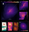 |
Fig. 1. Visualization of the entire dynamical range covered in our simulations. The figure displays data taken from the final snapshot of run G4. Panels a–d show the projected gas column density along the y direction across multiple scales, ranging from ≈9.35 × 10³ AU in panel a to 3 AU in panel d. Panels e–j are slices through the center of the domain along the y direction for panels e, g, and i, and along the z direction for panels f, h, and j. These display density (panels e and f), radiative flux (panels g and h), and temperature (panels i and j). The color bars in panels e and f are centered on the density of the inner disk’s shock front (≈1.5 × 10⁻⁹ g cm−3 at this snapshot). |
3.2. Protostellar breakup
We begin by describing the structure of the system shortly after the onset of the second gravitational collapse using Fig. 2. We use data from run G6 as an example, although the evolutionary sequence displayed here applies to all other runs as well. The top row of this figure (panels a–d) displays the local radiative flux, an excellent tracer of shock fronts. It is computed as
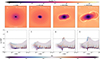 |
Fig. 2. Demonstration of the breakup of the protostar due to excess angular momentum. The data is taken from run G6. Each column represents a different time, where t = 0 marks the birth of the protostar. Panels a–d are slices along the z direction through the center of the domain that display the local radiative flux emanating from the cells (see Eq. (1)). The scale bar in panel a applies to panels b–d as well. The mass of the protostar at each snapshot is displayed in the top-right corners of panels a–d. Panels e–h display 2D histograms binning all the cells in our computational domain, which show the distribution of azimuthal velocities divided by |

where c is the speed of light, λ the Minerbo (1978) flux limiter, Er the radiative energy, ρ the gas density, and κR the Rosseland mean opacity. At a shock front, kinetic energy is converted into radiation and as such it is accompanied by an increase in radiative flux. Hence, this quantity prominently displays accretion shocks and spiral waves.
The bottom row of the figure (panels e–h) displays the azimuthal velocity2 distribution of all cells in our computational domain with respect to radius, which we have divided by the critical velocity beyond which the centrifugal force exceeds the radial component of the gravitational force:

where

Here, ϕ is the gravitational potential obtained through the Poisson equation.
Once the gas has completed its dissociation of H2 molecules and ample thermal pressure support is gathered, the second Larson core (i.e., the protostar) is formed. At birth (first column), the protostar is a thermally supported spherical object, and its azimuthal velocities are well below vcrit. A mere eight and a half days later (second column), the protostar has nearly doubled in mass, and an equatorial bulge is now visible in panel b. This is due to the fact that as the protostar accretes, it is also accumulating angular momentum. Nevertheless, it is still rotating below vcrit. A month later (third column), the outer shells of the protostar finally exceed vcrit, after which material spreads outward and transitions to a differential rotation profile in which the centrifugal force is now the main counterbalance to gravity. The sustained accretion ensures a constant flow of material within the protostar exceeding vcrit.
3.3. An embedded protostar
The expulsion of material by the protostellar surface will naturally lead to the formation of a circumstellar disk. Here, we study how such a disk grows and evolves while analyzing the accretion mechanism onto the protostar and the disk. To this end, we studied Fig. 3, which displays density slices through the center of the computational domain for run G1 at different times. The velocity streamlines are color coded with the local radial mass-flux −ρvr, where red colors denote inward transport of material, blue colors denote outward transport, and white signifies very little transport. The evolutionary sequence displayed here applies to all other runs.
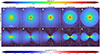 |
Fig. 3. Top-down (top row, panels a–e) and edge-on (bottom row, panels f–j) slices through the center of the domain of run G1 displaying density and velocity streamlines. The color coding in the velocity streamlines displays the local radial mass flux −ρvr. Each column displays a different epoch, where t = 0 (panels b and g) corresponds to the moment of protostellar breakup. The scale bar in panel a applies to all other panels. An animated version of this plot is available online. |
Panels a and f display the system once temperatures exceed 2000 K and the dissociation of H2 is triggered, where the gas spirals inward almost isotropically. The central region accumulates material quickly, and once ample thermal pressure support is gathered, the protostar forms. We display in panels b and g the structure of the system once the protostar reaches breakup velocity. As the protostar’s surface begins expelling material, a disk immediately forms afterward, and as time progresses, an increasing amount of material collides with the disk instead of the protostar, thus causing the former to grow significantly over time. Hereafter, we refer to this newly formed circumstellar disk as the inner disk (in accordance with the terminology of Machida & Matsumoto 2011). In panel d, we observed the development of spiral waves, which seem to have subsided into near-circular waves in panel e3 We note that during this phase, the accretion timescale of the disk (Md/Ṁd ∼ 10−2 M⊙/10−2 M⊙ yr−1 = 1 yr) is shorter than its dynamical timescale (2πRd/vϕ ∼ 2π × 1 AU/3 km s−1 ≈ 10 yr). This means that any angular momentum redistribution process within the inner disk occurs on longer timescales than accretion. Thus, accretion is the dominant process behind the expansion of the disk.
We now turn to studying the accretion process with the aid of the streamlines in Figs. 3 and 4, which displays the radial mass flux in slices through the center of the domain. In addition, we display unbroken velocity vector field streamlines in Fig. 5 at a curated moment. Although the polar regions initially bring a large amount of material to the central protostar, the polar reservoir of gas is quickly depleted and by t ≈ 268 days (fourth columns and onward of Figs. 3 and 4), very little mass is accreted through the poles. Indeed, most of the material landing at the protostellar surface is sliding on the inner disk’s surface, as its velocity component normal to the disk surface is not strong enough to break through the shock front. We note, however, that some material landing on the disk surface can sometimes break through the shock front and is then transported into the inner disk, as can be seen in panel b of Fig. 5. The previously mentioned spiral waves can be seen transporting material radially in panels d and e. This is more apparent in Fig. 6, which displays the radial mass flux averaged in radial bins and measured separately for both the upper layers of the disk and its main body for all our runs. One can see that in all runs and across all radii, the upper layers of the disk have a strictly positive radial mass flux, whereas the main body shows alternating inflows and outflows of material.
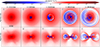 |
Fig. 4. Same as Fig. 3 but displaying only the local radial mass flux −ρvr in order to better demonstrate how accretion occurs in the star and inner disk system. An animated version of this plot is available online. |
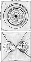 |
Fig. 5. Unbroken velocity vector field streamlines of run G1 at t ≈ 322 days after the birth of the inner disk illustrating the dynamics of accretion onto the disk and protostar in a top-down (panel a) and edge-on (panel b) view. The scale bar in panel b applies to panel a as well. An animated version of these streamlines, made using windmap (https://github.com/rougier/windmap) is available online. |
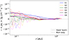 |
Fig. 6. Average radial mass flux measured in radial bins for runs G1 (blue), G2 (orange), G3 (green), G4 (red), G5 (black), and G6 (magenta) at a moment in time where the inner disk has reached ≈1 AU in radius. Only cells belonging to the inner disk were considered (see Appendix A for information on how the inner disk was defined). The solid lines represent measurements made on the upper layers of the disk, whereas the dashed lines represent measurements made in its main body. |
What is most visually striking from the edge-on views is the vertical extent of the disk: it is substantially flared, giving it the shape of a torus. This is more so apparent in the 3D rendering of the system displayed in Fig. 7. The inner disk’s surface (rendered in blue) completely engulfs the protostar (rendered in green). Figure 7 also displays the 3D velocity streamlines, which show that the material accreted through the poles carries with it angular momentum as the gas is spiraling inward. The cross-sectional slices in the figure display the radiative flux, which reveals shock fronts and spiral waves. Interestingly, there does not seem to be any shock fronts separating the protostar from the inner disk (barring the spiral waves). This means that the accretion shock envelopes both the protostar and the inner disk, and the two act as a continuous fluid system. As such, differentiating the protostar and the inner disk is rather difficult, but the rotational profiles seem to indicate that the protostar is in solid body rotation and the inner disk exhibits differential rotation4. All other runs have displayed an identical structure of the inner disk.
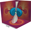 |
Fig. 7. Three-dimensional view of the inner disk and protostar at a moment in time when the former has reached ≈0.5 AU in radius. The blue structure is the surface of the inner disk. The inner r < 0.1 AU region has been cut out in order to reveal the flow onto the protostar (rendered in green). The white curves are velocity vector field streamlines launched along the poles to reveal polar accretion. The bottom, left, and right panels are cross sections through the center of the domain displaying the radiative flux. The visualized volume is 1.6 × 1.6 × 1.6 AU3. An animated version of this plot is available online. |
3.4. A convergent structure
We display in Figs. 8 and 9 the radiative flux in slices through the center of the domain for runs G1−G6 at a moment in time where the inner disk has reached a radius of ≈0.5 AU. We note the almost identical structure of the inner disk in all runs: it is toroidal and highly flared. We also note that run G3 (panels c and q) displays a strong eccentricity, as the outer disk that formed around the first Larson core in this run was already highly eccentric prior to the second collapse.
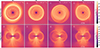 |
Fig. 8. Slices through the center of the domain for runs G1, G2, G3, and G4 (respectively first, second, third, and fourth columns) showing the local radiative flux in a top-down (top row, panels a–d) and edge-on (bottom row, panels e–h) view. The slices illustrate the structure of the accretion shock as well as the presence of spirals in the inner disk (see Eq. (1)). The scale bar in panels d and h apply to all other panels as well. The slices are shown at a moment in time where the inner disks have reached a radius of ≈0.5 AU. The mass of each inner disk is displayed in the top-right corners of panels a–d. |
In the top-down slices (panels a–d), we notice ripples in radiative flux. These are spiral waves which have relaxed into nearly circular perturbations. We note that runs G1 and G2 have stronger spirals waves (i.e., the radiative flux emanating from them is stronger) due to their higher mass. (For a more in-depth analysis of these spiral waves, see Sect. 3.6).
An interesting observation from panels e–h of Fig. 8 is the prominence of the radiative flux along the poles. Indeed, the polar region is much less dense than the equator, which causes the radiative flux to escape much more easily along this direction. This also causes the gas to heat up in the polar direction5.
3.5. Evolution
Having ascertained the structure of the system in the innermost regions following the second gravitational collapse, we follow the temporal evolution of the inner disk with the aid of Fig. 10. The properties of the inner disk once it has reached a radius of 1 AU are of particular interest, as that is the most commonly chosen sink radius.
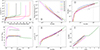 |
Fig. 10. Temporal analysis of the inner disk in all our runs. Blue is for G1, orange for G2, green for G3, red for G4, black for G5, and magenta for G6. Panel a provides the context in which the inner disk is born by displaying the central density’s evolution since the formation of the first Larson core (defined as the moment where ρc > 10−10 g cm−3). Panels b–e respectively display as a function of the inner disk’s equatorial radius Rd (analogous to time) the density of the inner disk’s equatorial shock front, the mass of the inner disk, the protostellar mass, and the specific angular momentum of the inner disk. Panel f displays the evolution of the inner disk radius with respect to time, where t = 0 marks the moment of birth of the inner disk. The gray dotted line in panels b–e marks Rd = 1 AU. (For information on how the inner disk was defined, see Appendix A). |
First, we point out the different evolutionary history of each simulation in panel a. This figure displays the maximum density in our computational domain as a function of time since the birth of the first core. The moment in which each curve exhibits a sharp rise in central density corresponds to the onset of the second gravitational collapse. Here, we observed clearly that simulations with higher initial amounts of angular momentum have a delayed onset of second collapse, as the additional centrifugal support significantly extends the first core’s lifetime by reducing its mass accretion rate. In runs G3, G4, G5, and G6, the first core lifetime is long enough for it to have a disk built around it such that the inner disk forms within a disk (Machida & Matsumoto 2011). Despite the differing evolutionary histories, the resulting properties of the inner disk, displayed in panels b, c, e, and f, show remarkable similarity. Indeed the temporal evolution of the inner disk equatorial radius Rd (panel f), shows very little spread. The specific angular momentum of the inner disks, displayed in panel e, also exhibit striking similarity. This shows that the amount of specific angular momentum in the inner disk is independent of the initial amount of angular momentum in the parent cloud core, a result that is in agreement with Wurster & Lewis (2020)’s non ideal MHD and hydro simulations. Furthermore, the entirety of the angular momentum budget of the first core is found within the inner disk and protostar after it is accreted.
The curves in panel c display the inner disk’s mass (Md), which exhibit the same evolutionary trend and Md(1 AU)∈[1.634 × 10⁻²; 2.755 × 10⁻²] M⊙. The mass of the protostar (panel d), although very similar in runs G1−G4, has runs G5−G6 as outliers since M* is about ⪆40% larger in these runs. Interestingly, M* also seems to be decreasing in most runs, meaning that the protostar is shedding its mass to the disk due to excess angular momentum. The notable exception is run G1, in which the protostar’s mass is increasing due to strong gravitational torques.
Finally, we turn our attention to panel b, which displays the density of the inner disk’s equatorial shock front (ρs). We measure this quantity along the equator since that is the region where most of the incoming mass flux lands on the inner disk (as shown in Fig. 3). As such, this quantity is an equivalent to the accretion threshold used in sink particles (nacc). We report ρs(1 AU)∈[5.35 × 10⁻¹⁰; 2 × 10⁻⁹] g cm−3. The most commonly adopted accretion threshold in the literature is 1.66 × 10⁻¹¹ g cm−3 (nacc = 1013 cm−3). We thus suggest higher values of nacc when possible for studies employing sink particles whose radius is 1 AU. However, we acknowledge that this can significantly increase the numerical cost of simulations, and thus might be too constraining for certain studies, particularly those that aim for very long temporal evolution.
The reason for such a convergence in the inner disk properties is the first core itself. As discussed in Ahmad et al. (2023), this hydrostatic object halts any inward accretion until temperatures can exceed the H2 dissociation temperature of 2000 K, after which the second collapse ensues. As such, the mass accretion rate asymptotically reaches  (∼10−2 M⊙ yr−1, Larson 1969; Penston 1969) independently of initial conditions, provided that a first core forms. The small spread we observed in Fig. 10 is the result of our turbulent initial conditions, as no discernible trend can be inferred from their differences. We expect the large-scale initial conditions to play a more significant role later on when the entirety of the first Larson core is accreted and that mass accretion rates onto the innermost regions are dictated by transport processes within the disk and by the infall of material onto said disk.
We note that in the case where an outer disk exists prior to the onset of a second collapse, the inner disk will simply merge with it (Machida & Matsumoto 2011). This was the case for runs G3, G4 and G5. The first core lifetime in runs G1 and G2 was not long enough for it to gather enough material around it to form a disk.
3.6. Gravitational stability of the inner disk
The existence of such a massive circumstellar disk naturally begs the question of whether it will undergo fragmentation or not. In order to determine the gravitational stability of the inner disk, we use the classical Toomre Q parameter (Toomre 1964):

where cs is the gas sound speed, Σ its surface density, and ω its epicyclic frequency, defined as
where Ω is the angular velocity of the gas. This parameter represents the ratio of the outward pointing forces on the gas, namely the centrifugal and pressure gradient forces, to the inward pointing gravitational force. If Q < 1, the disk is unstable and a fragmentation is likely. We measure the sound speed and the angular velocity by averaging along the vertical axis of the inner disk.
We display the real part of Q in top-down slices through the center of the domain for run G1 in Fig. 11 at curated moments. In panel a, we display the circumstellar disk at its birth, just after the protostar exceeded breakup velocity and began shedding its mass. This results in a ring of gas surrounding the protostar, whose Q value is above unity. In panel b, we display the system just prior to the onset of the first large amplitude spiral wave. Here, the Q parameter remains above unity in the innermost regions of the disk; however, an hourglass-shaped region has Q < 1 at slightly larger radii. The ratio of inner disk mass to protostellar mass has also increased by a factor ≈7. In panel c, a coherent two-armed spiral wave is launched from the center, and it grows radially as it is sheared apart by differential rotation when propagating outward. Finally, panels d and e show that these spiral waves relax into nearly circular ripples as a result of the increase in temperature. The Q values in panels b–e hovers around unity throughout the disk, meaning that the disk remains marginally stable against gravitational instabilities despite its high mass relative to that of the protostar. This is due to its very high temperature.
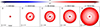 |
Fig. 11. Top-down slices through the center of the domain of run G1 displaying the real part of the Toomre Q parameter (see Eq. (4)) at different times. Here, t = 0 (panel a) corresponds to the moment of birth of the inner disk. Only cells belonging to the inner disk were used in the calculation of Q. The ratio of the inner disk mass to protostellar mass is displayed on the bottom left of each panel. The scale bar in panel a applies to all other panels. An animated version of this plot is available online. |
A recent numerical study by Brucy & Hennebelle (2021) has shown that the fragmentation barrier of disks is quite blurry; it is better described by a probabilistic approach and said probabilities strongly depend on how efficiently the disk is able to cool. As such, the fragmentation of the disk is also set by the cooling criterion. In our case, the inner disk is still strongly accreting, and a considerable amount of accretion energy is absorbed by the disk, particularly along the optically thick equator (this is shown in Sect. 5). This ensures that the inner disk remains hot and thus mostly stable against fragmentation despite its very high mass relative to the protostar. The primary regulator of the inner disk temperature during this phase is the endothermic dissociation of H2, which places γeff at ≈1.1.
4. Gas structure and kinematics
Herein, we provide a more quantitative analysis of the structure and kinematics of the inner disk with the aid of Fig. 12. Panels a–e of this figure display various quantities azimuthally averaged in radial bins in the equatorial region, where the equator was defined as the region in which θ/π ∈ [0.45; 0.55], where θ is the co-latitude. The curves are shown at a moment in time in which the inner disk has reached a radius of ≈1 AU.
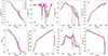 |
Fig. 12. Studying the structure and kinematics of the gas in our simulations. Panels a–e display a set of azimuthally averaged quantities along the equatorial regions with respect to radius, where the equator was defined as the region where θ/π ∈ [0.45; 0.55] at a moment in time where the inner disk has reached ≈1 AU in radius. Panel a displays the density, panel b shows the radial velocity, panel c presents the azimuthal velocity, panel d shows the specific angular momentum, and panel e presents the temperature. Panel f displays the enclosed angular momentum profile. Panel g displays the deviation from Keplerian rotation along the disk midplane. Panel h displays the column density profile of the inner disk, where non-disk cells were masked. |
Panel a displays the equatorial density curve, which exhibits a plateau in the innermost regions (r < 10−2 AU) and a power law tail6. This behavior has been described by all previous 3D studies in the literature that employ either pure hydro or non-ideal MHD. This density structure, as well as the radial velocity curves displayed in panel b, suggest that no discontinuity in the flow separates the protostar from the inner disk. The only way for us to differentiate the two is by studying the rotational behavior of the system: we observed an object in solid body rotation in the inner-most regions (j ∝ r2, panel d) and a transition to a differential rotation profile (panel c).
4.1. Deviations from Keplerian rotation
We observed a significant deviation from Keplerian rotation (vϕ ∝ r−0.5) in the inner disk. Indeed, it seems that vϕ ∝ r−0.3. In order to explain such a difference, one must start by analyzing the balance equation between the centrifugal, pressure, and gravitational forces (Pringle 1981; Lodato 2007):
where P is the thermal pressure. By assuming a radial density profile where ρ ∝ r−β and radial isothermality ( ), we may write
where cs is the gas sound speed. We may approximate gr from the column density profile of the inner disk:
where G is the gravitational constant and
Here, Σ is the disk’s surface density. We note that this is merely an analytical estimate of gr, which is different from the true potential computed in Eq. (3). Now let us assume a column density profile of Σ ∝ r−ξ. This means that the grr term in Eq. (7) scales with r−ξ + 1, whereas the  term scales with r−β(γ − 1) (T ∝ ργ − 1). From Fig. 12, we can write ξ ≈ 3/2 and β ≈ 3. Additionally, γ ≈ 1.1 in the inner disk (panel e of Fig. 12). Thus, grr ∝ r−0.5 and
  . This means that we may expect stronger deviations from Keplerian velocity at larger radii in the inner disk. At Rd = 1 AU, we have Md ∼ 10−2 M⊙ and cs ∼ 1 km s−1. As such,
  , and we thus expect the deviation from Keplerian rotation to be of the order of (vϕ − vK)/vK ≈ −20% (where
  ). Panel g of Fig. 12 shows us that these are reasonable approximations.
Note that what we call “Keplerian” rotation in the present paper is different from its commonly adopted meaning in the literature. Indeed, the literature defines the Keplerian velocity as  ; however, as the disk’s mass exceeds that of the protostar by up to a factor of seven, the measured deviations from vK, lit would be ∼100%.
4.2. Analytical description of the inner disk structure
Herein, we set out to provide an analytical description of the structure of the inner disk, which is rather exotic by virtue of its very high mass relative to that of the protostar, as well as its very high temperature. This is not meant to be a full analytical development, but rather, one that seeks to deepen our understanding of the structure witnessed in our simulations. Namely, we seek to understand why Σ ∝ r−3/2, and in turn provide an analytical prediction of nacc. To do so, we use as our starting point the important result shown in Sect. 3.6, namely that Q ≈ 1 throughout most of the inner disk. This allowed us to link the sound speed cs and the disk’s column density profile Σ through

We can write the following power-law descriptions of these two quantities
where we have made use of the fact that ρ ∝ r−β. We note that Ω is constrained by Σ through the equation
This allowed us to write
To describe Σ, one must thus first obtain the boundary values at r = R* and r = 1 AU. Since Σ and cs are linked through Eq. (10), this is equivalent to finding the boundary values of cs. Our simulations indicate β ≈ 3, and γ ≈ 1.1 in the inner disk. Hence, cs ∝ r−0.15. This allowed us to write
Since R* ∼ 10−2 AU,

This means that when traveling from the protostellar surface to r = 1 AU, cs reduces by a factor of approximately two. The temperature of the inner disk is ∼103 K, hence cs(1 AU)∼1 km s−1 and cs0 ∼ 2 km s−1. By using Eq. (10), we can link this boundary condition to ξ:
Numerically solving Eq. (18) for ξ such that (cs/cs0)2 ≈ 1/4 yields ξ ≈ 1.38 (with M* ∼ 10−3 M⊙), which is close to the value witnessed in most of our runs (≈3/2, panel h of Fig. 12).
Once we had a description of both Σ and cs, we could describe the density profile with the aim of predicting nacc as

where h is the disk scale height:

Thus, this analytical framework provides ρ(1 AU)≈5.37 × 10⁻¹⁰ g cm−3 (nacc ≈ 3.23 × 1014 cm−3, when considering a mean molecular weight of one). This result is within the bounds provided by the simulations ([5.35 × 10⁻¹⁰; 2 × 10⁻⁹] g cm−3), and thus we consider it to be satisfactory.
4.3. Radial transport within the inner disk
Once we had an analytical framework with which we could describe the inner disk, it was of interest to quantify the transport of material within it. More specifically, we wished to describe the transport processes using a simple alpha-disk model (Shakura & Sunyaev 1973) and compare it with the measured values within our simulations. A common approach in this regard is to measure the stress tensors induced by turbulent fluctuations and the self-gravity of the disk, respectively αR and αgrav (e.g., Lodato & Rice 2004; Brucy & Hennebelle 2021; Lee et al. 2021). However, in our case, we found these measurements difficult to interpret, as the disk is awash with eccentric motions (Lovascio et al., in prep.), turbulent eddies, spiral waves, and erratically infalling material (see for example Fig. 5), which resulted in unreliable values of αR and αgrav. Instead, we opted for a simpler approach in which we attempted to fit an approximate analytical description of the transport within the inner disk with the measured values of our simulations. The mass accretion rate at any given radius in our simulations can be obtained using
where ⟨vr⟩ is the vertically averaged radial velocity. We note that the majority of the inward transport of material occurs in the upper layers of the disk, as seen in Fig. 6. Along the midplane, material tends to spread outward, causing negative mass accretion rates. As such, when performing the vertical average of vr, we weighed vr in two different ways:
where zmin and zmax are respectively the minimal and maximal heights of the disk at a given radius and azimuth. ⟨vr⟩z will thus be biased by the infall in the upper layers of the disk, whereas ⟨vr⟩ρ will be biased by the dense midplane.
The analytical estimate of the mass accretion rate is (Shakura & Sunyaev 1973; Pringle 1981)
where ν is the effective viscosity of the inner disk

Here, αsh is the Shakura & Sunyaev (1973) alpha which dictates the vigour of radial mass transport. Using the equations developed in the previous section, we may write Eq. (24) as
We may obtain an estimate of the αsh parameter in Eq. (26) with the aid of Fig. 13, which displays the mass accretion rate in our simulations computed using Eq. (21) at a moment in time when the inner disk radius has reached ≈1 AU. We measure Ṁs using both ⟨vr⟩z (panel a) and ⟨vr⟩ρ (panel b). Using average stellar parameters reported in the figure caption, we over-plot Eq. (26) (solid gray lines). The figure shows that the vigour of inward transport varies across all radii, and in the case of runs G2-6, the outer layers (r > 0.2 AU) of the inner disk have negative mass accretion rates, meaning that material is mostly spreading outward. In panel b, we saw that the transport of material in the main body of the inner disk fluctuates wildly. Furthermore, any inward transport in this region consistently has lower mass accretion rates than in the upper layers of the disk (panel a). Indeed, the upper layers of the disk have a mass accretion rate that can be approximated by Eq. (26) with αsh ∼ 5 × 10⁻².
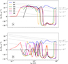 |
Fig. 13. Radial mass accretion rate within the inner disk for all runs (solid colored lines) as a function of cylindrical radius and computed using Eq. (21) at a moment in time when Rd has reached ≈1 AU. Only cells belonging to the inner disk were used in the computation of Ṁs. Panel a displays the measurements of Ṁs made using ⟨vr⟩z (Eq. (22)), whereas panel b displays the same measurements made using ⟨vr⟩ρ (Eq. (23)). The solid gray lines are analytical estimates of radial transport computed using Eq. (26), with αsh = 10−1 (top), 5 × 10⁻² (middle), and 10−2 (bottom). The other parameters for the solid gray lines are M* ≈ 7 × 10⁻³ M⊙; R* ≈ 3 × 10⁻² AU; cs0 ≈ 5 km s−1; β ≈ 3; ξ ≈ 3/2, and γ ≈ 1.1. |
We note, however, that Ṁs varies not only in space but also in time, and so the value of αsh reported here is not valid throughout the entirety of the class 0 phase. Indeed, once most of the remnants of the first Larson core are accreted, and that the mass accretion rate onto the star-disk system significantly reduces, this will inevitably cause a decrease in αsh, as Ṁs is mainly dominated by the infall and will thus drop by several orders of magnitude. We would thus have a disk whose angular momentum transport is very weak, with αsh ∼ [10−5; 10−3], but whose mass is significantly higher than that of the protostar. In addition, panel d of Fig. 10 shows that despite the inward transport of material within the inner disk, the protostellar mass is decreasing in most runs as a result of excess angular momentum. This allowed us to conclude that although the inner disk can be described by the physics of alpha disks, such a description is a first-order approximation whose results are not entirely reliable.
5. Radiative behavior
Although the protostar has not reached the temperatures required for fusion yet (> 106 K), it will dominate the radiative output of the system by virtue of its high temperature and its accretion luminosity. A quantitative analysis of said radiative behavior is seldom provided in the literature, and it is the purpose of this section.
To this end, we first begin by providing a qualitative overview of the radiative behavior of the system at medium (i.e., 102 AU) scales. As discussed previously, the structure of the accretion shock is rather complex, as it envelopes both the protostar and the inner disk. Nevertheless, the polar accretion shock, as seen in the bottom rows of Figs. 8 and 9, produces the majority of the radiative flux. In addition, the density cavity along the poles allows said radiation to escape much more easily than along the optically thick equator. This is reflected in Fig. 14, which displays the radiative flux emanating from each cell in edge-on slices across the center of our domain at curated moments for run G5. The protostar is born embedded within a disk that formed around the first Larson core (panel a). As time progresses, the radiation produced at the protostellar accretion shock escapes and brightens the polar regions significantly (panels b–d). However, the equatorial regions remain dark as the radiative flux struggles to pierce through the highly opaque disk. As such, the disk is almost unaffected by the protostar’s radiation.
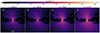 |
Fig. 14. Edge-on slices through the center of the domain displaying the local radiative flux at different times (see Eq. (1)). Here, t = 0 (panel a) corresponds to the moment of protostellar birth. The data is taken from run G5. The scale bar in panel a applies to all other panels. An animated version of this plot is available online. |
We now turn to providing a quantitative analysis of the radiative behavior of the protostar and inner disk. To do so, as in Vaytet et al. (2018), Bhandare et al. (2020), and Ahmad et al. (2023), we compare two quantities: the radiative flux just upstream of the accretion shock (Frad, see Eq. (1)), and the incoming accretion energy flux. However, since the shock front’s structure is complex, we measure these quantities in only four directions: north-south along the poles, and east-west along the equator (see panel a of Fig. 15):

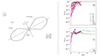 |
Fig. 15. Quantitative analysis of the radiative behavior of the accretion shock. Panel a is a schematic representation of the star and inner disk system, where the solid line is the location of the accretion shock that envelopes both the protostar and the disk. The dashed lines represent four rays launched from the center of the system along which the location of the accretion shock is found and its radiative efficiency measured just upstream from it (numbered red dots). The resulting measurements are presented in panels b and c. North and South (respectively solid and dashed lines in panel b and East and West (respectively solid and dashed lines in panel c are shown for all simulations. These display the polar and equatorial radiative efficiencies (respectively facc, pol and facc, eq; see Eqs. (31) and (32)). |
where R* (resp. Rd) is the protostellar (resp. inner disk) radius, E the gas internal energy, P its thermal pressure, and
This allowed us to define the radiative efficiency as

These are approximate measurements of the radiative efficiency of the accretion shock because the radiative flux also contains the cooling flux emanating from the protostellar interior, although the later remains smaller than that produced at the accretion shock because of the low temperature of the protostar (∼104 K) prior to deuterium burning.
We display in panels b and c of Fig. 15 the resulting measurements of facc, pol and facc, eq obtained through ray-tracing. A schematic drawing displaying the location at which each quantity was measured is presented in panel a. In contrast to spherically symmetrical calculations, the radiative efficiency of the accretion shock displays a strong anisotropy: the polar accretion shock (panel b) is much more efficient than its equatorial counterpart (panel c). Indeed, the polar shock front reaches supercriticality (facc, pol = 1) in less than 2.5 years for most runs, whereas facc, eq < 1 throughout all simulations. This is due to the polar density cavity that allows the accretion shock to shine into an optically thin medium, whereas the equatorial accretion shock remains optically thick due to the remnants of the first Larson core and the presence of an extended outer disk around it.
The drop in facc, eq seen in most runs (e.g., at t ≈ 1.2 yr for run G1) is due to the equatorial shock front expanding out of the opacity gap, a region where temperatures are high enough to sublimate dust (see Fig. 1 of Ahmad et al. 2023). This causes the shock front to shine into a region of higher opacity, which in turn reduces its luminosity. Eccentric inner disks can also cause an east-west anisotropy, as is most apparent in run G3. In contrast, we witness very minor anisotropies when comparing north-south radiative efficiencies.
The low radiative efficiency of the equatorial shock front has an important consequence on the structure of the inner disk: as it accretes, the majority of the accretion energy is dumped into its thermal budget, thus causing it to maintain a high temperature and to swell along the vertical extent.
6. Discussions
6.1. The star-disk structure
In the common star formation paradigm, the protostar is often seen as a standalone object wholly separate from the circumstellar disk due to an accretion shock separating the two. Our results show that such a boundary does not exist: the transition from the protostar to the inner disk is a smooth one, and the two act as a continuous fluid system. This means that until either torque mechanisms transport sufficient material inward, or a protostellar magnetosphere arises, the protostar and the inner disk will continue to behave as a continuous fluid system.
Unfortunately, obtaining observational constraints on the structure of the system in such a young and deeply embedded object is very difficult, but two recent studies by Laos et al. (2021) and Le Gouellec et al. (2024) seem to be offering hints on the accretion mechanism during the class 0 phase. Whereas Laos et al. (2021) argues for magnetospheric accretion similarly to class I objects by basing their arguments on the similar shapes of the Brγ line profiles, Le Gouellec et al. (2024) additionally analyzed the velocity profiles of these lines which exhibited clear differences. Based on this result, they concluded that the accretion mechanism in class 0 sources must be of a different nature. Additionally, they report very vigorous accretion unto the central regions. These observations are an indirect probe of the structure of the system following the second collapse. If a stellar magnetosphere cannot be inferred from them, then we argue that a structure similar to that described in this paper may be present.
6.2. Toward an eventual fragmentation
Although our analysis of the gravitational stability of the inner disk indicates that it is currently marginally stable against gravitational instabilities, it is also in a transient state in which it maintains an incredibly high temperature through accretion. This is by virtue of the low radiative efficiency of the inner disk’s shock front. The protostar, as shown in Sect. 5, contributes almost nothing to heating the inner disk because it is currently embedded within it and the majority of its radiative flux escapes along the poles. One can imagine that such a disk will inevitably cool down once accretion subsides, and thus would be much more prone to fragmentation. The high mass budget of the inner disk also indicates that such fragmentations can occur multiple times, and thus lead to the formation of multiple star systems, or perhaps of Jupiter-like planets in close proximity to the central star.
6.3. Caveats
Although the radiative-hydro approximation is valid for the timescales described here, this obviously cannot be the case on longer timescales, as the stellar magnetic field will undoubtedly increase once a dynamo process begins. Furthermore, the hot, dense, and highly turbulent inner disk may also generate a dynamo process (Balbus & Hawley 1991; Wardle 1999; Lesur et al. 2014; Riols & Latter 2019; Deng et al. 2020). The onset of strong magnetic fields will bring about outflows and jets, as well as induce strong magnetic torques that can transport material inward and also reduce the rotation rate of the protostar to observed values in more evolved systems (∼10% of breakup velocity, Hartmann & Stauffer 1989; Herbst et al. 2007). These will likely heavily influence the evolution of the system in the innermost regions. Nevertheless, the simulation presented in Machida & Basu (2019) was integrated for 2000 years after protostellar birth with non-ideal MHD, and their results seem to indicate that ρs(1 AU)∼10−9 g cm−3 (see their Fig. 13). Their protostar also seems to progressively separate from the inner disk (see panels m–p of their Fig. 5 and vr in their Fig. 11), likely as a result of magnetic torques. Although state of the art non-ideal MHD simulations indicate that thermal pressure support far outweighs its magnetic counterpart in circumstellar disks (e.g., Machida et al. 2010; Vaytet et al. 2018; Machida & Basu 2019; Lee et al. 2021), magnetic torques likely outweigh turbulent viscosity or gravitational torques (as quantified by Machida & Basu 2019).
In addition, although we notice relatively little spread in our results, more exhaustive constraints on the inner boundaries of circumstellar disks can be obtained by exploring a more varied range of M0, α, and βrot. This was not done due to computational constraints, as the simulations are expensive to run at such high resolution (each run used at least 100 000 CPU hours in total).
6.4. Consequences on global disk evolution scenarios
As a result of the high values of nacc hereby reported, the mass of circumstellar disks in numerical simulations may have been underestimated by about an order of magnitude (Hennebelle et al. 2020a). This appears to be inconsistent with observations of class 0 disks, which report lower disk masses of ∼10−2 M⊙ (Tobin et al. 2020). We note, however, that a recent study by Tung et al. (2024) has found that class 0 disk masses are routinely underestimated with current observational techniques. Nevertheless, the results indicate that the disk is very massive at birth, and naturally one must question how such a disk might evolve over time.
As such, we put forward two speculative evolutionary scenarios that we believe to be possible. The first scenario rests on the previously discussed fragmentation of the disk; as accretion subsides and the disk cools, it will become more prone to gravitational instabilities. Should the inner disk fragment, a significant amount of angular momentum could be extracted from the system.
Another scenario would rest on the strength of magnetic fields in the inner disk. Perhaps the results of current state of the art papers that report high thermal to magnetic pressure ratios are overestimating the strength of magnetic resistivities in the gas whose density exceeds first Larson core densities (ρ > 10−13 g cm−3), and thus would be underestimating the magnetic field strength within the protostar’s and inner disk’s precursor. This is in light of new studies (Lebreuilly et al. 2023; Kawasaki & Machida 2023; Tsukamoto et al. 2023; Vallucci-Goy et al., in prep.) that cast doubt on the validity of the MRN (Mathis-Rumple-Nordsiek, Mathis et al. 1977) dust size distribution used in said state of the art papers. In the case where the resistivities inside the first Larson core are overestimated, we would expect stronger coupling within the gas prior to hydrogen ionization. Although the ratio of thermal to magnetic pressure is still expected to greatly exceed unity within the inner disk, this would undoubtedly increase the strength of magnetic torques and cause a more central distribution of material, in which the protostar quickly exceeds the inner disk’s mass and separates itself from it. However, simulations employing MRN resistivities create disk radii in broad agreement with observational surveys (Maury et al. 2019; Tobin et al. 2020), in which the magnetic field truncates the disk radius at ∼101 AU. Perhaps the disk radii can serve as a lower bound on magnetic resistivities for low density gas, whereas the strength of magnetic fields in young stellar objects (∼103 G, Durney et al. 1993; Chabrier & Küker 2006) can serve as an upper bound on resistivities within the first Larson core.
6.5. Comparison with previous works
We now turn to comparing our results with previous calculations in the literature that have resolved the birth of the protostar and the inner disk structure described in this paper. Due to the very stringent time-stepping, only a handful of such studies exist. To our knowledge, the first report of the existence of a swollen disk-like structure around the second core is that of Bate (1998), who carried out their calculations using the SPH numerical method under the barotropic approximation. Saigo et al. (2008) later confirmed the existence of such a structure with their own barotropic calculations, this time using a nested-grid code. Although these papers do no have enough details presented for us to quantitatively compare our results, the description they provide of the structure of the second core and its surroundings seem to be qualitatively similar to ours. Following these two studies, Machida & Matsumoto (2011) led a detailed study of the inner disk under the barotropic approximation in which they include magnetic fields with ohmic dissipation, where they found qualitatively similar results to the hydro case. Notably, they report an inner disk mass of ∼10−2 M⊙, and a protostellar mass of ∼10−3 M⊙, in accordance with our results.
More recent studies include those of Wurster et al. (2018, 2022), Vaytet et al. (2018), Machida & Basu (2019), Wurster & Lewis (2020). The simulations presented in Vaytet et al. (2018) were also run with the RAMSES code while including magnetic fields. They reported the existence of a circumstellar disk around the protostar when including magnetic resistivities. They also reported that they could not resolve the shock front separating the protostar from the inner disk, but as we have demonstrated in this paper, such a shock front does not exist. The mass of the disk reported in their paper is ∼10−4 M⊙, which is to be expected given their short simulation time following protostellar birth (24 days) that results from stringent time-stepping.
As stated previously, Machida & Basu (2019) have also studied the inner disk, in which they were able to follow the calculations for a period of 2000 years following protostellar birth. Their results seem to indicate similar ratios of protostellar to disk mass than our paper, and the structure of their inner disk also seems to be similar to ours despite the presence of a magnetically launched outflow and a high velocity jet.
Finally, Wurster et al. (2018, 2021, 2022), Wurster & Lewis (2020) ran these calculations using SPH and all non-ideal MHD effects: ohmic dissipation, ambipolar diffusion, and the hall effect. They found the same disk structure following the second collapse phase. In contrast to Machida & Basu (2019), they report no high velocity jets and argue that magnetically launched outflows are circumstantial and depend on the initial turbulent velocity vector field, as well as the non-ideal effects at play. The only way in which we may quantitatively compare our results to theirs is through the protostellar mass, which seems to be ∼10−3 M⊙. The inner disk mass was not measured in these papers.
In summary, the circumstellar disk structure described in this paper is routinely found in previous papers simulating the second collapse in 3D. Although the quantitative details of the properties of said disk may differ due to different numerical methods and physical setups, it is guaranteed to be recovered in simulations that possess sufficient amounts of angular momentum in the first core. As such, the only simulations that do not recover it are those that make use of the ideal MHD approximation, which extracts too much angular momentum from the system and prevents the protostar from ever reaching breakup velocity.
7. Conclusion
We have carried out a set of high resolution 3D RHD simulations that self-consistently model the collapse of a 1 M⊙ dense molecular cloud core to stellar densities with the goal of studying the innermost (< 1 AU) regions. Our results are summarized as follows:
-
(i)
Following the second gravitational collapse, the protostar is formed through hydrostatic balance. Through accretion, the protostar accumulates angular momentum and reaches breakup velocity, after which it sheds some of its mass to form a hot, dense, and highly turbulent circumstellar disk, which we call the inner disk. The protostar is embedded within this disk, and no shock front separates the two. As accretion continues, the disk completely engulfs the protostar and spreads outward due to a combination of excess angular momentum and accretion. The disk mass exceeds that of the protostar by a factor of approximately seven, which means that the majority of the mass following the second collapse resides in the disk and its self-gravity dominates, with notable contributions from thermal pressure on its dynamics. In the case where an outer disk exists prior to the second collapse, this circumstellar disk forms within it, and the two merge after the inner disk spreads to sufficiently large radii.
-
(ii)
Despite the differing evolutionary histories at larger spatial scales, the star-disk structure formed after the onset of the second collapse is identical, with a small spread caused by the turbulent initial conditions. This is due to the formation of the first Larson core in all our simulations, a hydrostatic object that ensures that the second collapse occurs in approximately similar conditions.
-
(iii)
Accretion onto the protostar mainly occurs through material that slides on the disk’s surface, as polar accretion has a low-mass flux in comparison. Along the equator, material spreads outward due to excess angular momentum. Accretion onto the inner disk is highly anisotropic.
-
(iv)
The radiative emissions of the star-disk system are anisotropic. The radiative efficiency of the accretion shock is supercritical along the poles, whereas the inner disk’s equatorial shock front is subcritical and on the order of 10−3.
-
(v)
The density of the inner disk’s shock front at 1 AU (the most commonly used sink radius) is in the range of [5.35 × 10⁻¹⁰; 2 × 10⁻⁹] g cm−3, which is about an order of magnitude higher than the commonly used sink accretion threshold of 1.66 × 10⁻¹¹ g cm−3. Thus, we suggest higher accretion thresholds for studies employing sink particles whenever possible. We note, however, that our results correspond to very early times and may not be applicable throughout the entirety of the class 0 phase.
-
(vi)
In order to physically decouple the protostar from its disk and reduce its rotation rate to observed values, torque mechanisms need to transport a sufficient amount of angular momentum outward. Magnetic fields are likely to play this role.
These results reveal the structure and kinematics of the innermost regions of circumstellar disks, which are often omitted from simulations due to computational constraints. Although our results are valid for the timescales described here (< 6 years following protostellar birth), we expect magnetic fields to play a more significant role later on, particularly in creating powerful torques that transport material toward the protostar.
Movies
Movie 1 associated with Fig. 2 (figure_2) Access here
Movie 2 associated with Figs. 3 and 4 (figure_3_and_4) Access here
Movie 3 associated with Fig. 5 (figure_5_a) Access here
Movie 4 associated with Fig. 5 (figure_5_b) Access here
Movie 5 associated with Fig. 7 (figure_7) Access here
Movie 6 associated with Fig. 11 (figure_11) Access here
Movie 7 associated with Fig. 14 (figure_14) Access here
In the case of runs G1 and G2, no disk was formed at these scales prior to the onset of the second collapse. This is discussed further in Sect. 3.5.
The gravitational stability of the inner disk is discussed in Sect. 3.6.
See Appendix A for an overview of how each object was defined.
The radiative behavior of the system is studied in Sect. 5.
Acknowledgments
This work has received funding from the French Agence Nationale de la Recherche (ANR) through the projects COSMHIC (ANR-20-CE31-0009), DISKBUILD (ANR-20-CE49-0006), and PROMETHEE (ANR-22-CE31-0020). We have also received funding from the European Research Council synergy grant ECOGAL (Grant: 855130). We thank Ugo Lebreuilly, Anaëlle Maury, and Thierry Foglizzo for insightful discussions during the writing of this paper. The simulations were carried out on the Alfven super-computing cluster of the Commissariat à l’Énergie Atomique et aux énergies alternatives (CEA). Post-processing and data visualization was done using the open source Osyris (https://github.com/osyris-project/osyris) package. 3D visualizations were done using the open-source PyVista (https://docs.pyvista.org/version/stable/) package (Sullivan & Kaszynski 2019).
References
- Ahmad, A., González, M., Hennebelle, P., & Commerçon, B. 2023, A&A, 680, A23 [NASA ADS] [CrossRef] [EDP Sciences] [Google Scholar]
- Badnell, N. R., Bautista, M. A., Butler, K., et al. 2005, MNRAS, 360, 458 [Google Scholar]
- Balbus, S. A., & Hawley, J. F. 1991, ApJ, 376, 214 [Google Scholar]
- Bate, M. R. 1998, ApJ, 508, 508 [Google Scholar]
- Bate, M. R. 2010, MNRAS, 404, L79 [NASA ADS] [Google Scholar]
- Bate, M. R. 2011, MNRAS, 417, 2036 [CrossRef] [Google Scholar]
- Bate, M. R. 2012, MNRAS, 419, 3115 [NASA ADS] [CrossRef] [Google Scholar]
- Bate, M. R. 2018, MNRAS, 475, 5618 [Google Scholar]
- Bate, M. R., Bonnell, I. A., & Price, N. M. 1995, MNRAS, 277, 362 [Google Scholar]
- Bate, M. R., Tricco, T. S., & Price, D. J. 2014, MNRAS, 437, 77 [NASA ADS] [CrossRef] [Google Scholar]
- Bhandare, A., Kuiper, R., Henning, T., et al. 2020, A&A, 638, A86 [NASA ADS] [CrossRef] [EDP Sciences] [Google Scholar]
- Bleuler, A., & Teyssier, R. 2014, MNRAS, 445, 4015 [Google Scholar]
- Brucy, N., & Hennebelle, P. 2021, MNRAS, 503, 4192 [NASA ADS] [CrossRef] [Google Scholar]
- Chabrier, G., & Küker, M. 2006, A&A, 446, 1027 [NASA ADS] [CrossRef] [EDP Sciences] [Google Scholar]
- Commerçon, B., Teyssier, R., Audit, E., Hennebelle, P., & Chabrier, G. 2011, A&A, 529, A35 [NASA ADS] [CrossRef] [EDP Sciences] [Google Scholar]
- Commerçon, B., Debout, V., & Teyssier, R. 2014, A&A, 563, A11 [NASA ADS] [CrossRef] [EDP Sciences] [Google Scholar]
- Commerçon, B., González, M., Mignon-Risse, R., Hennebelle, P., & Vaytet, N. 2022, A&A, 658, A52 [NASA ADS] [CrossRef] [EDP Sciences] [Google Scholar]
- Deng, H., Mayer, L., & Latter, H. 2020, ApJ, 891, 154 [Google Scholar]
- Durney, B. R., De Young, D. S., & Roxburgh, I. W. 1993, Sol. Phys., 145, 207 [NASA ADS] [CrossRef] [Google Scholar]
- Ferguson, J. W., Alexander, D. R., Allard, F., et al. 2005, ApJ, 623, 585 [Google Scholar]
- González, M., Vaytet, N., Commerçon, B., & Masson, J. 2015, A&A, 578, A12 [NASA ADS] [CrossRef] [EDP Sciences] [Google Scholar]
- Grudić, M. Y., Guszejnov, D., Offner, S. S. R., et al. 2022, MNRAS, 512, 216 [CrossRef] [Google Scholar]
- Hartmann, L., & Stauffer, J. R. 1989, AJ, 97, 873 [Google Scholar]
- Hennebelle, P., Commerçon, B., Lee, Y.-N., & Charnoz, S. 2020a, A&A, 635, A67 [NASA ADS] [CrossRef] [EDP Sciences] [Google Scholar]
- Hennebelle, P., Commerçon, B., Lee, Y.-N., & Chabrier, G. 2020b, ApJ, 904, 194 [NASA ADS] [CrossRef] [Google Scholar]
- Herbst, W., Eislöffel, J., Mundt, R., & Scholz, A. 2007, in Protostars and Planets V, eds. B. Reipurth, D. Jewitt, & K. Keil, 297 [Google Scholar]
- Joos, M., Hennebelle, P., & Ciardi, A. 2012, A&A, 543, A128 [CrossRef] [EDP Sciences] [Google Scholar]
- Kawasaki, Y., & Machida, M. N. 2023, MNRAS, 522, 3679 [NASA ADS] [CrossRef] [Google Scholar]
- Krumholz, M. R., Klein, R. I., McKee, C. F., Offner, S. S. R., & Cunningham, A. J. 2009, Science, 323, 754 [Google Scholar]
- Kuiper, R., Klahr, H., Beuther, H., & Henning, T. 2010, ApJ, 722, 1556 [NASA ADS] [CrossRef] [Google Scholar]
- Laos, S., Greene, T. P., Najita, J. R., & Stassun, K. G. 2021, ApJ, 921, 110 [NASA ADS] [CrossRef] [Google Scholar]
- Larson, R. B. 1969, MNRAS, 145, 271 [Google Scholar]
- Lebreuilly, U., Hennebelle, P., Colman, T., et al. 2021, ApJ, 917, L10 [NASA ADS] [CrossRef] [Google Scholar]
- Lebreuilly, U., Vallucci-Goy, V., Guillet, V., Lombart, M., & Marchand, P. 2023, MNRAS, 518, 3326 [Google Scholar]
- Lebreuilly, U., Hennebelle, P., Maury, A., et al. 2024a, A&A, 683, A13 [NASA ADS] [CrossRef] [EDP Sciences] [Google Scholar]
- Lebreuilly, U., Hennebelle, P., Colman, T., et al. 2024b, A&A, 682, A30 [NASA ADS] [CrossRef] [EDP Sciences] [Google Scholar]
- Lee, Y.-N., Charnoz, S., & Hennebelle, P. 2021, A&A, 648, A101 [NASA ADS] [CrossRef] [EDP Sciences] [Google Scholar]
- Le Gouellec, V. J. M., Greene, T. P., Hillenbrand, L. A., & Yates, Z. 2024, ApJ, 966, 91 [NASA ADS] [CrossRef] [Google Scholar]
- Lesur, G., Kunz, M. W., & Fromang, S. 2014, A&A, 566, A56 [NASA ADS] [CrossRef] [EDP Sciences] [Google Scholar]
- Lodato, G. 2007, Nuovo Cimento Rivista Serie, 30, 293 [NASA ADS] [Google Scholar]
- Lodato, G., & Rice, W. K. M. 2004, MNRAS, 351, 630 [Google Scholar]
- Machida, M. N., & Basu, S. 2019, ApJ, 876, 149 [CrossRef] [Google Scholar]
- Machida, M. N., & Matsumoto, T. 2011, MNRAS, 413, 2767 [NASA ADS] [CrossRef] [Google Scholar]
- Machida, M. N., Inutsuka, S.-I., & Matsumoto, T. 2006, ApJ, 647, L151 [NASA ADS] [CrossRef] [Google Scholar]
- Machida, M. N., Inutsuka, S.-I., & Matsumoto, T. 2007, ApJ, 670, 1198 [NASA ADS] [CrossRef] [Google Scholar]
- Machida, M. N., Inutsuka, S.-I., & Matsumoto, T. 2008, ApJ, 676, 1088 [CrossRef] [Google Scholar]
- Machida, M. N., Inutsuka, S.-I., & Matsumoto, T. 2010, ApJ, 724, 1006 [NASA ADS] [CrossRef] [Google Scholar]
- Machida, M. N., Inutsuka, S.-I., & Matsumoto, T. 2011, PASJ, 63, 555 [NASA ADS] [CrossRef] [Google Scholar]
- Machida, M. N., Inutsuka, S.-I., & Matsumoto, T. 2014, MNRAS, 438, 2278 [NASA ADS] [CrossRef] [Google Scholar]
- Mathis, J. S., Rumpl, W., & Nordsieck, K. H. 1977, ApJ, 217, 425 [Google Scholar]
- Maury, A. J., André, P., Testi, L., et al. 2019, A&A, 621, A76 [NASA ADS] [CrossRef] [EDP Sciences] [Google Scholar]
- Mignon-Risse, R., González, M., & Commerçon, B. 2021a, A&A, 656, A85 [NASA ADS] [CrossRef] [EDP Sciences] [Google Scholar]
- Mignon-Risse, R., González, M., Commerçon, B., & Rosdahl, J. 2021b, A&A, 652, A69 [NASA ADS] [CrossRef] [EDP Sciences] [Google Scholar]
- Mignon-Risse, R., González, M., & Commerçon, B. 2023, A&A, 673, A134 [NASA ADS] [CrossRef] [EDP Sciences] [Google Scholar]
- Minerbo, G. N. 1978, J. Quant. Spectr. Radiat. Transf., 20, 541 [NASA ADS] [CrossRef] [Google Scholar]
- Oliva, A., & Kuiper, R. 2023, A&A, 669, A80 [NASA ADS] [CrossRef] [EDP Sciences] [Google Scholar]
- Penston, M. V. 1969, MNRAS, 144, 425 [NASA ADS] [CrossRef] [Google Scholar]
- Pringle, J. E. 1981, ARA&A, 19, 137 [NASA ADS] [CrossRef] [Google Scholar]
- Riols, A., & Latter, H. 2019, MNRAS, 482, 3989 [Google Scholar]
- Saigo, K., Tomisaka, K., & Matsumoto, T. 2008, ApJ, 674, 997 [NASA ADS] [CrossRef] [Google Scholar]
- Saumon, D., Chabrier, G., & van Horn, H. M. 1995, ApJS, 99, 713 [NASA ADS] [CrossRef] [Google Scholar]
- Semenov, D., Henning, T., Helling, C., Ilgner, M., & Sedlmayr, E. 2003, A&A, 410, 611 [NASA ADS] [CrossRef] [EDP Sciences] [Google Scholar]
- Shakura, N. I., & Sunyaev, R. A. 1973, A&A, 24, 337 [NASA ADS] [Google Scholar]
- Sullivan, C., & Kaszynski, A. 2019, J. Open Source Softw., 4, 1450 [NASA ADS] [CrossRef] [Google Scholar]
- Teyssier, R. 2002, A&A, 385, 337 [CrossRef] [EDP Sciences] [Google Scholar]
- Tobin, J. J., Sheehan, P. D., Megeath, S. T., et al. 2020, ApJ, 890, 130 [CrossRef] [Google Scholar]
- Tomida, K., Tomisaka, K., Matsumoto, T., et al. 2013, ApJ, 763, 6 [NASA ADS] [CrossRef] [Google Scholar]
- Tomida, K., Okuzumi, S., & Machida, M. N. 2015, ApJ, 801, 117 [Google Scholar]
- Toomre, A. 1964, ApJ, 139, 1217 [Google Scholar]
- Tsukamoto, Y., & Machida, M. N. 2013, MNRAS, 428, 1321 [NASA ADS] [CrossRef] [Google Scholar]
- Tsukamoto, Y., Iwasaki, K., Okuzumi, S., Machida, M. N., & Inutsuka, S. 2015, MNRAS, 452, 278 [NASA ADS] [CrossRef] [Google Scholar]
- Tsukamoto, Y., Machida, M. N., & Inutsuka, S.-I. 2023, PASJ, 75, 835 [NASA ADS] [CrossRef] [Google Scholar]
- Tung, N.-D., Testi, L., Lebreuilly, U., et al. 2024, A&A, 684, A36 [NASA ADS] [CrossRef] [EDP Sciences] [Google Scholar]
- Vaytet, N., Chabrier, G., Audit, E., et al. 2013, A&A, 557, A90 [NASA ADS] [CrossRef] [EDP Sciences] [Google Scholar]
- Vaytet, N., Commerçon, B., Masson, J., González, M., & Chabrier, G. 2018, A&A, 615, A5 [NASA ADS] [CrossRef] [EDP Sciences] [Google Scholar]
- Vorobyov, E. I., Skliarevskii, A. M., Elbakyan, V. G., et al. 2019, A&A, 627, A154 [NASA ADS] [CrossRef] [EDP Sciences] [Google Scholar]
- Wardle, M. 1999, MNRAS, 307, 849 [NASA ADS] [CrossRef] [Google Scholar]
- Whitehouse, S. C., & Bate, M. R. 2006, MNRAS, 367, 32 [NASA ADS] [CrossRef] [Google Scholar]
- Wurster, J., & Lewis, B. T. 2020, MNRAS, 495, 3807 [CrossRef] [Google Scholar]
- Wurster, J., Bate, M. R., & Price, D. J. 2018, MNRAS, 481, 2450 [NASA ADS] [CrossRef] [Google Scholar]
- Wurster, J., Bate, M. R., & Bonnell, I. A. 2021, MNRAS, 507, 2354 [NASA ADS] [CrossRef] [Google Scholar]
- Wurster, J., Bate, M. R., Price, D. J., & Bonnell, I. A. 2022, MNRAS, 511, 746 [CrossRef] [Google Scholar]
Appendix A: Defining the protostar and inner disk in our simulations
The definition of the protostar in our simulations is rather semantic, as it is not a separate object from the inner disk. We use the same criterion as Vaytet et al. (2018) for defining the protostar: it is simply the gas whose density is above 10−5 g cm−3. We note that in Vaytet et al. (2018), the authors mention that they do not have enough resolution to resolve the protostellar accretion shock separating it from the circumstellar disk, although as we have shown in Sect. 3.2, such a discontinuity does not exist.
In order to define the inner disk, none of the criteria currently used in the literature were adequate in our case, mostly due to our use of turbulent initial conditions. Additionally, in some simulations, the second collapse occurred within a larger-scale disk, which further complicated our disk selection criterion. Inspired by Joos et al. (2012), we used the following criterion:
where ρs is the density of the inner disk’s equatorial shock front, obtained at each snapshot through ray-tracing. This criterion ensures that no cells currently undergoing the second gravitational collapse phase are selected and that sufficient angular momentum is present in the gas to qualify as a disk. The third item in this criterion states that ρ < 10−5 g cm−3, but this is again an arbitrary choice to separate the protostar from its circumstellar disk.
All Figures
|
Fig. 1. Visualization of the entire dynamical range covered in our simulations. The figure displays data taken from the final snapshot of run G4. Panels a–d show the projected gas column density along the y direction across multiple scales, ranging from ≈9.35 × 10³ AU in panel a to 3 AU in panel d. Panels e–j are slices through the center of the domain along the y direction for panels e, g, and i, and along the z direction for panels f, h, and j. These display density (panels e and f), radiative flux (panels g and h), and temperature (panels i and j). The color bars in panels e and f are centered on the density of the inner disk’s shock front (≈1.5 × 10⁻⁹ g cm−3 at this snapshot). |
| In the text | |
|
Fig. 2. Demonstration of the breakup of the protostar due to excess angular momentum. The data is taken from run G6. Each column represents a different time, where t = 0 marks the birth of the protostar. Panels a–d are slices along the z direction through the center of the domain that display the local radiative flux emanating from the cells (see Eq. (1)). The scale bar in panel a applies to panels b–d as well. The mass of the protostar at each snapshot is displayed in the top-right corners of panels a–d. Panels e–h display 2D histograms binning all the cells in our computational domain, which show the distribution of azimuthal velocities divided by |
| In the text | |
|
Fig. 3. Top-down (top row, panels a–e) and edge-on (bottom row, panels f–j) slices through the center of the domain of run G1 displaying density and velocity streamlines. The color coding in the velocity streamlines displays the local radial mass flux −ρvr. Each column displays a different epoch, where t = 0 (panels b and g) corresponds to the moment of protostellar breakup. The scale bar in panel a applies to all other panels. An animated version of this plot is available online. |
| In the text | |
|
Fig. 4. Same as Fig. 3 but displaying only the local radial mass flux −ρvr in order to better demonstrate how accretion occurs in the star and inner disk system. An animated version of this plot is available online. |
| In the text | |
|
Fig. 5. Unbroken velocity vector field streamlines of run G1 at t ≈ 322 days after the birth of the inner disk illustrating the dynamics of accretion onto the disk and protostar in a top-down (panel a) and edge-on (panel b) view. The scale bar in panel b applies to panel a as well. An animated version of these streamlines, made using windmap (https://github.com/rougier/windmap) is available online. |
| In the text | |
|
Fig. 6. Average radial mass flux measured in radial bins for runs G1 (blue), G2 (orange), G3 (green), G4 (red), G5 (black), and G6 (magenta) at a moment in time where the inner disk has reached ≈1 AU in radius. Only cells belonging to the inner disk were considered (see Appendix A for information on how the inner disk was defined). The solid lines represent measurements made on the upper layers of the disk, whereas the dashed lines represent measurements made in its main body. |
| In the text | |
|
Fig. 7. Three-dimensional view of the inner disk and protostar at a moment in time when the former has reached ≈0.5 AU in radius. The blue structure is the surface of the inner disk. The inner r < 0.1 AU region has been cut out in order to reveal the flow onto the protostar (rendered in green). The white curves are velocity vector field streamlines launched along the poles to reveal polar accretion. The bottom, left, and right panels are cross sections through the center of the domain displaying the radiative flux. The visualized volume is 1.6 × 1.6 × 1.6 AU3. An animated version of this plot is available online. |
| In the text | |
|
Fig. 8. Slices through the center of the domain for runs G1, G2, G3, and G4 (respectively first, second, third, and fourth columns) showing the local radiative flux in a top-down (top row, panels a–d) and edge-on (bottom row, panels e–h) view. The slices illustrate the structure of the accretion shock as well as the presence of spirals in the inner disk (see Eq. (1)). The scale bar in panels d and h apply to all other panels as well. The slices are shown at a moment in time where the inner disks have reached a radius of ≈0.5 AU. The mass of each inner disk is displayed in the top-right corners of panels a–d. |
| In the text | |
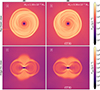 |
Fig. 9. Same as Fig. 8 but for runs G5 and G6 (respectively first and second columns). |
| In the text | |
|
Fig. 10. Temporal analysis of the inner disk in all our runs. Blue is for G1, orange for G2, green for G3, red for G4, black for G5, and magenta for G6. Panel a provides the context in which the inner disk is born by displaying the central density’s evolution since the formation of the first Larson core (defined as the moment where ρc > 10−10 g cm−3). Panels b–e respectively display as a function of the inner disk’s equatorial radius Rd (analogous to time) the density of the inner disk’s equatorial shock front, the mass of the inner disk, the protostellar mass, and the specific angular momentum of the inner disk. Panel f displays the evolution of the inner disk radius with respect to time, where t = 0 marks the moment of birth of the inner disk. The gray dotted line in panels b–e marks Rd = 1 AU. (For information on how the inner disk was defined, see Appendix A). |
| In the text | |
|
Fig. 11. Top-down slices through the center of the domain of run G1 displaying the real part of the Toomre Q parameter (see Eq. (4)) at different times. Here, t = 0 (panel a) corresponds to the moment of birth of the inner disk. Only cells belonging to the inner disk were used in the calculation of Q. The ratio of the inner disk mass to protostellar mass is displayed on the bottom left of each panel. The scale bar in panel a applies to all other panels. An animated version of this plot is available online. |
| In the text | |
|
Fig. 12. Studying the structure and kinematics of the gas in our simulations. Panels a–e display a set of azimuthally averaged quantities along the equatorial regions with respect to radius, where the equator was defined as the region where θ/π ∈ [0.45; 0.55] at a moment in time where the inner disk has reached ≈1 AU in radius. Panel a displays the density, panel b shows the radial velocity, panel c presents the azimuthal velocity, panel d shows the specific angular momentum, and panel e presents the temperature. Panel f displays the enclosed angular momentum profile. Panel g displays the deviation from Keplerian rotation along the disk midplane. Panel h displays the column density profile of the inner disk, where non-disk cells were masked. |
| In the text | |
|
Fig. 13. Radial mass accretion rate within the inner disk for all runs (solid colored lines) as a function of cylindrical radius and computed using Eq. (21) at a moment in time when Rd has reached ≈1 AU. Only cells belonging to the inner disk were used in the computation of Ṁs. Panel a displays the measurements of Ṁs made using ⟨vr⟩z (Eq. (22)), whereas panel b displays the same measurements made using ⟨vr⟩ρ (Eq. (23)). The solid gray lines are analytical estimates of radial transport computed using Eq. (26), with αsh = 10−1 (top), 5 × 10⁻² (middle), and 10−2 (bottom). The other parameters for the solid gray lines are M* ≈ 7 × 10⁻³ M⊙; R* ≈ 3 × 10⁻² AU; cs0 ≈ 5 km s−1; β ≈ 3; ξ ≈ 3/2, and γ ≈ 1.1. |
| In the text | |
|
Fig. 14. Edge-on slices through the center of the domain displaying the local radiative flux at different times (see Eq. (1)). Here, t = 0 (panel a) corresponds to the moment of protostellar birth. The data is taken from run G5. The scale bar in panel a applies to all other panels. An animated version of this plot is available online. |
| In the text | |
|
Fig. 15. Quantitative analysis of the radiative behavior of the accretion shock. Panel a is a schematic representation of the star and inner disk system, where the solid line is the location of the accretion shock that envelopes both the protostar and the disk. The dashed lines represent four rays launched from the center of the system along which the location of the accretion shock is found and its radiative efficiency measured just upstream from it (numbered red dots). The resulting measurements are presented in panels b and c. North and South (respectively solid and dashed lines in panel b and East and West (respectively solid and dashed lines in panel c are shown for all simulations. These display the polar and equatorial radiative efficiencies (respectively facc, pol and facc, eq; see Eqs. (31) and (32)). |
| In the text | |
Current usage metrics show cumulative count of Article Views (full-text article views including HTML views, PDF and ePub downloads, according to the available data) and Abstracts Views on Vision4Press platform.
Data correspond to usage on the plateform after 2015. The current usage metrics is available 48-96 hours after online publication and is updated daily on week days.
Initial download of the metrics may take a while.