| Issue |
A&A
Volume 675, July 2023
BeyondPlanck: end-to-end Bayesian analysis of Planck LFI
|
|
|---|---|---|
| Article Number | A7 | |
| Number of page(s) | 19 | |
| Section | Astronomical instrumentation | |
| DOI | https://doi.org/10.1051/0004-6361/202244061 | |
| Published online | 28 June 2023 | |
BEYONDPLANCK
VII. Bayesian estimation of gain and absolute calibration for cosmic microwave background experiments
1
Institute of Theoretical Astrophysics, University of Oslo, Blindern, Oslo, Norway
e-mail: eirik.gjerlow@astro.uio.no
2
INAF-Osservatorio Astronomico di Trieste, Via G.B. Tiepolo 11, Trieste, Italy
3
Dipartimento di Fisica, Università degli Studi di Milano, Via Celoria, 16, Milano, Italy
4
INAF-IASF Milano, Via E. Bassini 15, Milano, Italy
5
INFN, Sezione di Milano, Via Celoria 16, Milano, Italy
6
Planetek Hellas, Leoforos Kifisias 44, Marousi, 151 25
Greece
7
Department of Astrophysical Sciences, Princeton University, Princeton, NJ, 08544
USA
8
Jet Propulsion Laboratory, California Institute of Technology, 4800 Oak Grove Drive, Pasadena, CA, USA
9
Department of Physics, University of Helsinki, Gustaf Hällströmin katu 2, Helsinki, Finland
10
Helsinki Institute of Physics, University of Helsinki, Gustaf Hällströmin katu 2, Helsinki, Finland
11
Computational Cosmology Center, Lawrence Berkeley National Laboratory, Berkeley, CA, USA
12
Haverford College Astronomy Department, 370 Lancaster Avenue, Haverford, PA, USA
13
Max-Planck-Institut für Astrophysik, Karl-Schwarzschild-Str. 1, 85741 Garching, Germany
14
Dipartimento di Fisica, Università degli Studi di Trieste, Via A. Valerio 2, Trieste, Italy
Received:
19
May
2022
Accepted:
13
October
2022
We present a Bayesian calibration algorithm for cosmic microwave background (CMB) observations as implemented within the global end-to-end BEYONDPLANCK framework and applied to the Planck Low Frequency Instrument (LFI) data. Following the most recent Planck analysis, we decomposed the full time-dependent gain into a sum of three nearly orthogonal components: one absolute calibration term, common to all detectors, one time-independent term that can vary between detectors, and one time-dependent component that was allowed to vary between one-hour pointing periods. Each term was then sampled conditionally on all other parameters in the global signal model through Gibbs sampling. The absolute calibration is sampled using only the orbital dipole as a reference source, while the two relative gain components were sampled using the full sky signal, including the orbital and Solar CMB dipoles, CMB fluctuations, and foreground contributions. We discuss various aspects of the data that influence gain estimation, including the dipole-polarization quadrupole degeneracy and processing masks. Comparing our solution to previous pipelines, we find good agreement in general, with relative deviations of −0.67% (−0.84%) for 30 GHz, 0.12% (−0.04%) for 44 GHz and −0.03% (−0.64%) for 70 GHz, compared to Planck PR4 and Planck 2018, respectively. We note that the BEYONDPLANCK calibration was performed globally, which results in better inter-frequency consistency than previous estimates. Additionally, WMAP observations were used actively in the BEYONDPLANCK analysis, which both breaks internal degeneracies in the Planck data set and results in an overall better agreement with WMAP. Finally, we used a Wiener filtering approach to smoothing the gain estimates. We show that this method avoids artifacts in the correlated noise maps as a result of oversmoothing the gain solution, which is difficult to avoid with methods like boxcar smoothing, as Wiener filtering by construction maintains a balance between data fidelity and prior knowledge. Although our presentation and algorithm are currently oriented toward LFI processing, the general procedure is fully generalizable to other experiments, as long as the Solar dipole signal is available to be used for calibration.
Key words: cosmic background radiation / cosmology: observations / early Universe / inflation / methods: data analysis / methods: statistical
© The Authors 2023
 Open Access article, published by EDP Sciences, under the terms of the Creative Commons Attribution License (https://creativecommons.org/licenses/by/4.0), which permits unrestricted use, distribution, and reproduction in any medium, provided the original work is properly cited.
This article is published in open access under the Subscribe to Open model. Subscribe to A&A to support open access publication.
1. Introduction
Cosmic microwave background (CMB) anisotropies are among the most important observables that have been made available to cosmologists, and accurate determinations of their statistical properties has been a main goal for a multitude of collaborations and experiments over the last three decades (e.g., Smoot et al. 1992; de Bernardis et al. 2000; Kovac et al. 2002; Bennett et al. 2013; Planck Collaboration I 2020, and references therein). The BEYONDPLANCK project (BeyondPlanck Collaboration 2023) is an initiative aimed at establishing a common multi-experiment analysis platform that supports global end-to-end Bayesian analysis of raw time-ordered data (TOD) produced by such experiments, as well as seamless propagation of low-level uncertainties into all high-level products, including frequency and component maps, the CMB angular power spectra, and cosmological parameters. As a first demonstration, we applied this framework to the Planck LFI data, as presented in this and a suite of companion papers.
A fundamentally important step in any CMB analysis pipeline is photometric calibration – the process of mapping the instrument readout to the incoming physical signal. In general, this procedure involves comparing some specific feature in the measured data with a known calibration model, for instance, the CMB dipole or astrophysical foreground signal (or both), or by comparing the total measured power with a reference load with a known physical temperature (e.g., Planck Collaboration V 2016).
The multiplicative factor that processes the conversion between the sky signal and detector readout is called the gain. This factor typically depends on the local environment of the detectors, such as the ambient temperature, and is therefore in principle different for each sample. However, as long as the detectors are thermally stable on reasonably long timescales, it is usually a good approximation to assume that the gain is constant over some short period of time or at least that it is smoothly varying in time. For instance, the WMAP team adopted and fitted a six-parameter model for the gain, using housekeeping data such as focal plane temperature measurements to interpolate over time (Jarosik et al. 2007; Hinshaw et al. 2009; Greason et al. 2012). For LFI, we assume that the gain factor is constant throughout each Planck pointing period (PID) – the timescale over which the satellite scans a given “circle” on the sky; these last roughly an hour each. We also assume that the gain is varying smoothly between neighboring PIDs, except during a small set of events during which the instrument was actively modified by the mission control center, for instance, during cooler maintenance.
The Planck LFI Data Processing Centre (DPC; Planck Collaboration II 2014; Planck Collaboration V 2016; Planck Collaboration II 2020) used an onboard 4 K reference load to support the 30 GHz calibration for the early results, while for the other channels, and for all channels in later releases, they relied primarily on the CMB dipole signal. Gain fluctuations and correlations were modeled and suppressed by boxcar averaging over a signal-to-noise dependent window size. The Planck HFI DPC (Planck Collaboration VIII 2014, 2016; Planck Collaboration III 2020) also used the CMB dipole signal for gain estimation, but in this case they assumed a constant gain factor throughout the whole mission, relying on the excellent thermal stability of the Planck instrument. Apparent gain variations were instead assumed to arise from non-linearities in the analog-to-digital conversion module, which then allowed for a deterministic correction. A similar approach has also been adopted by the recent SROLL2 re-analysis initiative (Delouis et al. 2019). We refer to the latest DPC maps as Planck 2018.
In the most recent official analysis (Planck PR41; Planck Collaboration Int. LVII 2020), the Planck team adopted the LFI gain model for all channels up to and including the 857 GHz channel. A novelty introduced in that analysis, however, was a decomposition of the gain factor into two nearly orthogonal components: an absolute (or baseline) gain factor, which was assumed to be constant for the entire mission, and a detector-specific gain mismatch factor that could vary both in time and between detectors. This approach allowed estimation of each component separately, using calibrators that are better suited to each component. For example, the low signal-to-noise (but well-understood) orbital dipole was used to calibrate the absolute gain factor due to the long integration time involved in estimating this particular component. Solving for all relevant factors was then performed jointly with other relevant quantities.
In this paper, we adopt the Planck PR4 approach, decomposing the full gain into the above-mentioned components, and we estimate these jointly with all other parameters in the full model. Thus, the main novel feature presented in this paper is the integration of the gain estimation procedure within a larger Gibbs framework, as summarized by BeyondPlanck Collaboration (2023), which performs a joint estimation of all relevant parameters in a statistically consistent manner, including the CMB and astrophysical foreground sky signal.
The rest of the paper is structured as follows: in sect. 2, we aim to build intuition regarding gain estimation, presenting the general data model that we use and highlighting various important features of this model, as applied to real-world LFI observations. Next, in Sect. 3 we describe our main gain estimation procedure, which is validated through simulations in Sect. 4, before showing our results in Sect. 5 and making a comparison with those derived by other pipelines. Finally, we present our summary in Sect. 6, with a view toward future experiments and applications.
2. Data and modeling considerations
We start our presentation with a general discussion of the gain-related data model and how to account for various complications that arise when fitting it to real-world data.
2.1. Data model
As described by BeyondPlanck Collaboration (2023), the main goal of the BEYONDPLANCK analysis framework is to develop an end-to-end Bayesian analysis platform for CMB data, starting from raw time-ordered data. In this context, Bayesian analysis implies mapping out the posterior distribution; that is, given a set of observed data, d, and a theoretical model parameterized by a set of parameters, θ, the posterior distribution is given by:
where P(d ∣ θ) is referred to as the likelihood function, which quantifies the probability of observing the actual data for a given set of parameters, while P(θ) is the so-called prior distribution, which encodes whatever we believe about the parameters prior to any observations. Although informative priors are used in other parts of the BEYONDPLANCK pipeline, in this paper the prior is mostly be used as an explicitly Bayesian approach for incorporating smoothing of the raw gain solutions (see Sect. 3.5). The denominator, P(d), is called the evidence and is only important when comparing different models. In our case, it is a normalization factor with respect to the model parameter θ and we neglect it in the following.
As for most Bayesian problems, the key step in our approach is therefore to write down an explicit parametric model for the observed data from a given detector, dt, i, where t is the index denoting the sample2, and i is the index denoting the detector in question. In the current analysis, we adopt the following high-level model:
where  and
and  are correlated and white noise, respectively, gt, i is the gain factor, and
  denotes the total signal. Here,
  is given in kelvin, while dt, i is the instrument readout, which is measured in volts, meaning that the unit for gt, i becomes [V/K]. The total signal can further be decomposed into:
In this expression, P is the pointing matrix, which contains the mapping between the pointing direction the instrument, p and the sample index t; Bsymm, Basymm, and B4π denote convolution with the symmetric, asymmetric, and full 4π beams, respectively, which quantify the fraction of the total signal coming from direction p′ when the instrument is pointing towards p; ssky is the sky signal (including the solar dipole); sorb is the orbital dipole (to be discussed below); and sfsl represents signal leakage through the far-sidelobes. Solar System objects are either flagged at the TOD level (e.g., planets) or neglected (e.g., zodiacal light emission), following the same procedure as the official Planck LFI processing (Planck Collaboration II 2020). For further details regarding any of these objects, we refer the interested reader to BeyondPlanck Collaboration (2023) and references therein.
The main topic of the current paper is estimating gt, i. In this respect, it is important to note that all other free parameters in the data model, including  and
and  , are also unknown, and must be estimated jointly with gt, i. Casting this statement into Bayesian terms, we wish to sample from the posterior distribution given by3
Specifically, the aim is to model the “global” state of the instrument and data and to map out the probability of various points in parameter space by sampling from this distribution. This may at first glance seem like a intractable problem. However, a central component of the BEYONDPLANCK framework is parameter estimation through Gibbs sampling. According to the theory of Gibbs sampling, samples from a joint posterior distribution may be drawn by iteratively sampling from all conditional distributions. In other words, the process of instrumental calibration in the BEYONDPLANCK framework is reduced to sampling from P(g ∣ stot, sorb ncorr, …, d), meaning that when sampling the gain, we may assume that the sky signal and correlated noise parameters are perfectly known. And likewise, when sampling the sky signal or correlated noise parameters, we may assume that the gain is perfectly known. The correlations between these various parameters are then probed by performing hundreds or thousands of iterations of this type.
Thus, for the purposes of calibration alone, we do not need to be concerned with many aspects that indirectly affect the gain, such as CMB dipole or correlated noise estimation (Planck Collaboration II 2014; Planck Collaboration V 2016; Planck Collaboration II 2020). Instead, we are only concerned with defining an adequate model for g, and expressing this in a way that minimizes degeneracies with parameters in the Gibbs chain.
As discussed above, the gain is generally not constant in time. A very conservative (and somewhat naïve) model would therefore be to assume that the gain is in fact different for every sample t. However, this model clearly does not take into account our full knowledge about the instrument (Planck Collaboration XXVIII 2014). In particular, we do know that the gain is expected to correlate with the detector temperature, and this temperature does not change significantly on timescales of just one sample. Instead, based on available housekeeping data, a good assumption is that the gain is constant within a given pointing period (PID or “scan”) – which is defined as a collection of samples measured over a period of about an hour, during which the instrument spins about its axis once per minute while keeping the spin axis vector stationary. Between each scan, the instrument performs a slight adjustment of the satellite spin axis, ensuring that new sky areas are covered in consecutive pointing periods.
To reflect the assumption of constant gain within each scan, we rewrite our data model as follows:
where q now denotes PID. Thus, t is used to indicate a specific sample, while q represents a collection of samples.
From Eq. (5), we immediately note the presence of two important degeneracies, involving the sky signal and noise, respectively. If we attempt to fit for g, stot, and ncorr simultaneously, without knowing anything about any of them, we see that a given solution, say,  , results in an identical goodness-of-fit as another solution
  , as long as we have either:

or

In other words, the gain is multiplicatively degenerate with the signal and additively degenerate with the correlated noise. Such degeneracies are mainly a computational problem, since with two degenerate parameters in a Gibbs chain, exploring the resulting distributions takes a much larger number of samples than for uncorrelated parameters. A main topic of this paper is how to break these degeneracies in a statistically self-consistent and computationally efficient manner.
2.2. Absolute versus relative gain calibration
So far, we have been talking about the calibration of a given detector in isolation, which relates to what we call “absolute” calibration. Absolute calibration refers to correctly determining the “true” value of the gain and is important for accurately determining the emitted intensity of astrophysical components, such as the CMB.
Another closely related concept is “relative” calibration4, which quantifies calibration differences between radiometers. Because of Planck ’s scanning strategy, which only provides weak cross-linking5 (Planck Collaboration I 2011), it is impossible to estimate the three relevant Stokes parameters (the intensity, I, and two linear polarization parameters: Q and U) independently for each detector. Rather, the polarization signal is effectively determined by considering pairwise differences between detector measurements, while properly accounting for their relative polarization angle differences at any given time. Therefore, any instrument characterization error that induces spurious detector differences will be partially interpreted by the analysis pipeline as a polarization signal. If our relative gain calibration is wrong, such differences will be introduced.
Given the high sensitivity of current and future CMB experiments, the gain must be estimated to a fractional precision better than 𝒪(10−3) for robust CMB temperature analysis and better than 𝒪(10−4) for a robust polarization analysis. Accurate relative calibration is thus even more important than accurate absolute calibration and this does (as discussed in the next section) indeed inform the choices we make on how to estimate these two types of calibration.
2.3. The solar and orbital CMB dipoles
One of the most powerful ways to break the signal-gain degeneracy mentioned in the previous section is to observe a source of known brightness. If that source happens to be significantly stronger than other sources in the same area of the sky, we could fix  in Eq. (5) and the gain would essentially be determined by the ratio of the data to the known source brightness.
Unfortunately, the number of available astrophysical calibration sources that may be useful for CMB calibration purposes is very limited, given the stringent requirements discussed in Sect. 2.2. For instance, the brightness temperature of individual planets within the Solar system is only known to about 5% (Planck Collaboration VIII 2016), while only a few other local sources are known with a precision better than 1%.
The key exception is the CMB dipole. The peculiar velocity of the Planck satellite relative to the CMB rest frame induces a strong apparent dipole on the sky due to the Doppler effect. Specifically, photons having an anti-parallel velocity relative to the satellite motion are effectively blue-shifted, while photons with a parallel velocity are redshifted.
It is useful to decompose the peculiar spacecraft velocity into two components; the motion of the Solar system relative to the CMB rest frame, vsolar, and the orbital motion of the Planck satellite relative to the Solar system barycenter, vorbital. Thus, the total velocity of the satellite relative to the CMB rest frame is vtot = vsolar + vorbital. Taking into account the full expression for the relativistic Doppler effect, the induced dipole is expressed as:
where β = vtot/c, and γ = (1 − |β|2)−1/2. The total dipole is time dependent because of the motion of the satellite over the course of the mission. We can similarly define a Solar dipole, ssolar(x) and an orbital dipole, sorb(x, t), which are induced by only the Solar and orbital velocities alone, respectively.
Both dipoles play crucial roles in CMB calibration; the orbital dipole for absolute calibration and the Solar dipole for relative calibration.
Starting with the orbital dipole, we note that this depends only on the satellite’s velocity with respect to the Sun. This is exceedingly well measured through radar observations, and known with a precision better than 1 cm s−1 (Godard et al. 2009). For an orbital speed of 30 km s−1, this results in an overall relative precision better than 𝒪(10−6). However, Eq. (8) also depends on the CMB monopole, which is measured by COBE-FIRAS to 2.72548 K ± 0.57 mK (Fixsen 2009), corresponding to a relative uncertainty of 0.02% or 𝒪(10−4). Thus, the absolute calibration of any current and future CMB experiment cannot be determined with a higher absolute precision than 𝒪(10−4) until a next-generation CMB spectral distortion experiment, for instance PIXIE (Kogut et al. 2011), is launched. Still, this precision is more than sufficient for Planck calibration purposes.
The second CMB dipole component corresponds to the Sun’s motion with respect to the CMB rest frame. While this velocity is intrinsically unknown, one may estimate this from the relative amplitude of the Solar and orbital dipoles. This is illustrated in Fig. 1, which compares the orbital and Solar dipole signals (blue and black curves) with contributions from Galactic foreground emission and instrumental noise at 30 GHz for about three minutes of time-ordered observations. The Solar dipole is effectively determined by the relative amplitude ratio between the black and blue curves in this figure.
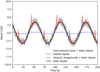 |
Fig. 1. Comparison of different contributions to the time-ordered data seen by Planck at 30 GHz, for a PID whose spin orientation is close to perpendicular to the dipole axis. The blue and black curves show the orbital and Solar CMB dipoles, respectively. The red and grey lines show the Solar CMB dipole with galactic foregrounds and instrumental noise added, respectively. |
Based on this approach, the most recent Planck analyses have determined that the Solar CMB dipole amplitude is about 3.36 mK, corresponding to Solar velocity of about 370 km s−1 (Planck Collaboration I 2020; Planck Collaboration Int. LVII 2020). For comparison, large-scale CMB polarization fluctuations typically exhibit variations smaller than 𝒪(1 μK) (Planck Collaboration IV 2020) and, consequently, the relative calibration of different detectors must be better than 𝒪(10−4) to avoid significant contamination of the polarization signal by the Solar CMB dipole. Achieving this level of precision in the presence of correlated noise, Galactic foregrounds, far sidelobe contamination, and other sources of systematic uncertainties is the single most difficult challenge associated with large-scale CMB polarization science.
2.4. Degeneracy between the CMB temperature dipole and polarization quadrupole
In Sect. 2.1 we noted that the gain is multiplicatively degenerate with the signal, and additively degenerate with the noise. Within this broad categorization, there are also some particularly important gain-signal degeneracies that are worth highlighting and perhaps the most prominent example is that with respect to the CMB polarization quadrupole. To illustrate this, we consider the case in which two detectors report different CMB dipole amplitude signals and we attempt to explain how such a difference might be explained. One possibility is a calibration mismatch, namely, that the absolute calibration of one or both detectors is misestimated.
Another possible explanation could be a large polarization CMB quadrupole signal. Due to the scanning strategy adopted by Planck, in which the same ring is observed repeatedly for one hour, a polarization quadrupole can easily appear with a dipolar signature, depending on the particular phase orientation of the mode in question. This is illustrated in Fig. 2. The black thick line shows the CMB temperature dipole as a function of time, while the colored thin lines show three random polarization quadrupole simulations, all observed with the Planck scanning strategy. Out of the three random quadrupole simulations, two have a time-domain behaviour that very closely mimics the CMB temperature dipole, and in the presence of noise and instrumental effects, it would be exceedingly difficult to distinguish between the two models.
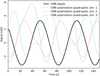 |
Fig. 2. Comparison of the CMB temperature dipole (thick black line) observed through the Planck scanning strategy with three random polarization quadrupole simulations (thin colored lines); the latter have been scaled by a factor of 104 for visualization purposes. |
This is a perfect recipe for a degenerate system, and one that carries the potential of contaminating any large-scale polarization reconstruction. It is, however, important to note that this particular degeneracy appears with a very specific morphology, and affects only a handful of spatial polarization modes, as defined by projecting the CMB Solar dipole onto the Planck scanning strategy. Recognizing the importance of this degeneracy, previous Planck analyses have adopted different strategies of resolving the issue. For instance, both the Planck 2018 and Planck PR4 analyses have opted to disregard the CMB polarization component completely during the calibration phase (Planck Collaboration II 2016, 2020; Planck Collaboration Int. LVII 2020). This may be at least partially justified for LFI on theoretical grounds by noting that the CMB polarization variance on large angular scales predicted by current best-fit ΛCDM models is ≲0.1 μK2, which is comparable to, or below, the overall noise. For the significantly more sensitive HFI instrument, this assumption is not adequate, and the recent Planck PR4 analysis therefore explicitly estimates a transfer function to account for this effect (Planck Collaboration Int. LVII 2020).
In the following, we adopt a slightly different strategy: We include the CMB polarization component in the calibration procedure, using the current sample in the Gibbs chain. In order to break the above-mentioned degeneracy, we replace the polarization quadrupole of the CMB map with a random value drawn from the best-fit ΛCDM model, using a value of  . Thus, we marginalize over this component and propagate the uncertainties introduced by this naturally into the Gibbs samples. We expect the combined effect of this addition to be negligible, because of the low value of the ΛCDM prediction, and as shown in Brilenkov et al. (2023) the gain estimation is unaffected by this marginalization.
2.5. Processing masks and PID selection
The Gibbs sampling framework used by BEYONDPLANCK requires an explicit parametric model that describes CMB, foregrounds, and the instrument. If this model turns out to be an insufficient representation of the actual data, the Gibbs sampling framework will attempt to fit eventual modeling errors using the parameters that are at its disposal. Ideally, such unexplained contributions should end up as an excess residual in r = d − gstot − ntot, but in practice they often also contaminate the other model parameters, such as the CMB. The correlated noise, ncorr, represents a set of such parameters that, because of their relatively unconstrained and global structure, end up absorbing a wide range of modeling errors, as discussed by Ihle et al. (2023). Furthermore, as already noted in Sect. 2.1, there is a tight degeneracy between the correlated noise and the gain, and ncorr is therefore a sensitive monitor for gain errors. Figure 3 illustrates this in terms of one arbitrarily selected 30 GHz ncorr sample from the main BEYONDPLANCK analysis (BeyondPlanck Collaboration 2023). The left column shows such a sample in the default model, in which the gain is allowed to vary from PID to PID, while the right column shows the same when enforcing a time-independent gain. While the maps in the left column are visually dominated by scan-aligned random stripes, as expected for ncorr, the maps in the right column (in particular the top row) show large excesses with a dipolar pattern along each Planck scanning ring. This is the archetypal signature of gain modeling errors, and this clearly demonstrates the need for a time-variable gain model. At the same time, there is also a clear quadrupolar pattern in the default configuration, with a positive excess along the Galactic plane and a negative excess near the Galactic poles. This structure is visually consistent with a near sidelobe modeling residual, in the sense that the Galactic foreground signal is slightly over-smoothed compared to the prediction of the nominal beam model, and the resulting residual is picked up by the correlated noise component. This is not surprising, considering that about 1% of the full LFI 30 GHz beam solid angle is unaccounted for in the GRASP beam model (Planck Collaboration II 2020), and some of this missing power may be in the near sidelobes. Fortunately, we also see from the same plot that the impact of this effect is modest and accounts for only about 1 μK at 30 GHz.
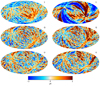 |
Fig. 3. Correlated noise maps for the 30 GHz channel in a Gibbs chain that includes (left panel) or neglects (right panel) gain time-dependencies. All maps are smoothed to a common resolution of 2.5° FWHM. |
More generally, because we have an incomplete understanding of both the instrument and the microwave sky, modeling errors will, at some level, always be a concern when estimating both gain and correlated noise. Furthermore, these modeling errors will typically be stronger near the Galactic plane or bright compact sources, where foreground uncertainties are large. For this reason, it is customary to apply a processing mask while estimating these quantities, omitting the parts of the sky that are least understood from the analysis. In BEYONDPLANCK, we define processing masks based on data-minus-signal residual maps for each frequency (Ihle et al. 2023), which are shown in Fig. 4.
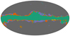 |
Fig. 4. Processing masks used in gain and correlated noise estimation for each frequency channel. The allowed 30 GHz sky fraction (blue) is 0.73, the 44 GHz sky fraction (green) is 0.81, and the 70 GHz sky fraction (red) is 0.77. |
In addition, as discussed by Basyrov et al. (2023), we also exclude a number of PIDs from the main analysis, for similar reasons as for applying processing masks. Most of these PIDs, however, do not correspond to particularly problematic areas of the sky, but rather to unmodeled instrumental changes or systematic errors, such as cooler maintenance or major satellite maneuvers. Excluded PIDs will show up as gaps in all PID plots in this paper.
2.6. Breaking degeneracies through multi-experiment analysis
As described in BeyondPlanck Collaboration (2023), BEYONDPLANCK includes as part of its data selection several external data sets that are necessary to break fundamental degeneracies within the model. One particularly important example in this respect is the inclusion of low-resolution WMAP polarization data. In the same way that the WMAP experiment was unable to measure a few specific polarization modes on the sky due to peculiarities in its scanning strategy (Jarosik et al. 2007), Planck is also unable constrain some modes as defined by its scanning strategy (Planck Collaboration II 2020). However, because the WMAP and Planck scanning strategies are intrinsically very different, their degenerate modes are not the same, and, therefore all sky modes may be measured to high precision when analyzing both data sets jointly.
This is explicitly demonstrated in Sect. 5.4, where we compare the BEYONDPLANCK sky maps to those derived individually from each experiment. The morphology of these frequency difference maps correspond very closely to the correction templates produced respectively by the WMAP and Planck teams (Jarosik et al. 2007; Planck Collaboration II 2020), and BEYONDPLANCK is statistically consistent with both data sets. Agreement is a direct and natural consequence of performing a joint fit, and there is no need for additional explicit template corrections for BEYONDPLANCK.
At the same time, it is also important to note that only the Planck LFI data are currently modeled in terms of time-ordered data, whereas the WMAP sky maps and noise covariance matrices are analyzed as provided by the WMAP team. Therefore, if there should be unknown systematics present in WMAP, those errors will necessarily also propagate into the various BEYONDPLANCK products. An important near-future goal is therefore to integrate also the WMAP time-ordered data into this framework. This work is already on-going, as discussed by Watts et al. (2023), but a full WMAP TOD-based analysis lies beyond the scope of the current work.
3. Methodology
As discussed in Sect. 2.1, our main goal in this paper is to draw samples from P(g ∣ stot, ncorr, d, …), the conditional distribution of g given all other parameters. In this section, we describe each of the various steps involved in this process.
3.1. Correlated noise degeneracies and computational speed-up
Before we present our main sampling algorithms for g, we recall from Sect. 2.1 that g is additively degenerate with ncorr. In a Gibbs sampling context, strong degeneracies lead to very long Markov correlation lengths as the Gibbs sampler attempts to explore the degenerate space between the two parameters. In order to save computing power and time, it is therefore better to sample g and ncorr jointly, such that for a given iteration of the main Gibbs chain, we instead sample directly from P(g, ncorr ∣ stot, d, …)6. It is important to note that this does not break the degeneracy between the gain and correlated noise, which, for instance, a strict prior on the correlated noise might achieve; rather, this process simply makes use of the fact that the sampling efficiency for two degenerate parameters is much better when sampling them jointly rather than conditionally.
A joint sample may be produced by means of uni-variate distributions through the definition of a conditional distribution:

Thus, sampling from the joint distribution P(g, ncorr ∣ stot, d, …) is equivalent to first sampling g from its marginal distribution with respect to ncorr, P(g ∣ stot, d, …), and then subsequently sampling ncorr from its conditional distribution with respect to g, P(ncorr ∣ g, stot, d, …). These two steps must be performed immediately after one another or else we would introduce an inconsistency in the Gibbs chain with respect to the other parameters.
We note that P(ncorr ∣ g, stot, d, …) is unchanged compared to the original Gibbs prescription, and no changes are required to sample from that particular distribution (see Ihle et al. 2023, for more details on this sampling process). When it comes to P(g ∣ stot, d, …), we refer to Appendix A.2 of BeyondPlanck Collaboration (2023), whose sampling equations we use throughout this paper. We note that the data model used in that appendix is the same general form as Eq. (5), and that sampling from P(g ∣ stot, d, …) is exactly analogous to what is shown in that appendix, as long as we make the identification n → ncorr + nwn. As the covariance matrix of a sum of independent Gaussian variables (ncorr and nwn) is also Gaussian, with a covariance matrix given by the sum of the individual covariance matrices, we can in what follows use the results of the above-mentioned appendix to sample from P(g ∣ stot, d, …) as long as we let N → Ncorr + Nwn.
Computationally speaking, sampling from P(g ∣ stot, d, …) instead of P(g ∣ stot, ncorr, d, …) is numerically equivalent to a more expensive noise covariance matrix evaluation7. To mitigate this additional cost, we note that the gain is assumed to be slowly varying in time, and, in particular, constant within each PID. All time-domain operations may therefore be carried out using co-added low-resolution data with negligible loss of precision. In practice, all TOD operations are in the following carried out at a sample rate of 1 Hz, leading to a computational speed-up of about two orders of magnitude.
3.2. Absolute gain calibration with the orbital dipole
Next, we recall (see Sect. 2.1) that the gain is multiplicatively degenerate with the total sky signal. At the same time, we note that the orbital CMB dipole is known to exquisite precision and this particular component is therefore the ideal calibrator for CMB satellite experiments. However, its relatively low amplitude as compared with instrumental noise renders it incapable of tracking short-term gain variations, and when fit jointly with astrophysical foregrounds, it is also not sufficiently strong to determine relative calibration differences between detectors at the precision required for large-scale polarization reconstruction. Therefore, to minimize sensitivity to potential residual systematic and modeling errors, it is advantageous to estimate the absolute calibration using the orbital dipole alone, but use the full signal model (including the bright Solar CMB dipole) when estimating relative and time-dependent gain variations.
This motivates splitting the gain into two components:
where g0 is now independent of both time and detectors, following Planck Collaboration Int. LVII (2020). Our goal is then to use only the orbital CMB dipole to estimate g0, and later use the full sky signal to estimate γq, i. Thus, with this reparametrization, we go from sampling from P(g ∣ stot, d, …) to sampling from P(g0, γ ∣ stot, d, …). As usual, drawing samples from this joint distribution can be done by Gibbs sampling, so that we first sample g0 from P(g0 ∣ γ, stot, d, …) and then γ from P(γ ∣ g0, stot, d, …).
We should note that estimating g0 using only the orbital dipole formally represents a violation of the Gibbs formalism, as we no longer draw this particular parameter from its exact conditional distribution. This is one of many examples for which we “buy” stability with respect to systematic errors at the price of increased statistical uncertainties. This is similar to the application of a processing mask when estimating the zero-levels of a CMB sky map (e.g., Planck Collaboration Int. XLVI 2016) or fitting correlated noise parameters using only a sub-range of all available temporal frequencies (e.g., Ihle et al. 2023). In all such cases, parts of the data are disregarded in order to prevent potential systematic errors from contaminating the parameter in question.
For the split in Eq. (10) to be valid, we must ensure that ∑q, iγq, i = 0, such that γq, i represents only deviations from the absolute calibration. For technical reasons, it turns out that this is easier to do if we also reparametrize γq, i,
where Δgi represents the detector-specific constant gain, and δgq, i denotes deviations from Δgi per scan. We can then separately enforce ∑iΔgi = 0 and ∑qδgq, i = 0 for each detector i, which is computationally cheaper than enforcing both constraints simultaneously.
Thus, we split the gain into three nearly independent variables and we explore their joint distribution by Gibbs sampling. The overarching goal for this section is thus to derive sampling algorithms for each of the three associated conditional distributions:


We then consider each of these in turn.
3.3. Sampling the absolute calibration, g0
To sample the absolute calibration using the orbital dipole alone, we need to define a data model that depends only on g0 and sorb. We do this by first subtracting the full signal model as defined by the current joint parameter state, and then add back only the orbital dipole term:
Here  denotes the absolute gain at the current iteration in the Gibbs chain, i.e., before drawing a new value for g0.
As noted earlier, working with this residual and using the previous sample of g0 to estimate the current sample does represent a breaking of the Gibbs formalism, since the statistically exact residual for g0 would be

However, in this case we would also be calibrating g0 on the total sky signal instead of just the orbital dipole. Thus, we trade mathematical rigour and statistical uncertainties for stronger robustness with respect to systematic effects.
As discussed in Sect. 3.1, the noise term in Eq. (15) includes both correlated and white noise, and the appropriate covariance matrix is therefore N = Ncorr + Nwn. Given this fact, Eq. (15) corresponds to a simple univariate Gaussian model as a function of g0, and the appropriate sampling algorithm is discussed in Appendix A.2 of BeyondPlanck Collaboration (2023). Applying that general procedure to our special case, we may write the following sampling equation for  8
8
where η ∼ N(0, 1) is a random number drawn from a standard normal distribution. Here (and elsewhere) a T superscript indicates the matrix transpose operator. The first term in this equation is the mean of the distribution P(g0 ∣ ri, Ni), while the second term ensures that g0 has the correct variance.
3.4. Sampling detector-dependent calibration
For Δgi, we proceed similarly as with g0, with two exceptions. First, Δgi now represents the relative calibration between detectors, and, as discussed in Sect. 2.1, we need to use a stronger calibration signal than the orbital dipole to avoid significant polarization leakage. Secondly, we have to impose the constraint ∑iΔgi = 0.
We start by defining the following residual,

for each detector. This equation is structurally similar to Eq. (15), with the main difference being that the total sky signal, which is dominated by the Solar dipole, is retained on the right-hand side. Otherwise, Eq. (18) still represents a Gaussian model, and we should be able to proceed similarly as for g0 when drawing from the conditional distribution. We do, however, need to ensure that ∑iΔgi = 0, and this significantly impact the form of the target distribution. The numerically most convenient method for imposing such a constraint is through the method of Lagrange multipliers.
In general, the method of Lagrange multipliers allows the user to minimize a function f(x) under some set of constraints that may be formulated as g(x) = 0. Without these constraints, one would of course determine x by solving df/dx = 0. With additional external constraints, however, it is convenient to instead define the so-called Lagrangian,

and set the corresponding partial derivatives with respect to x and λ equal to zero. It is readily seen that ∂ℒ/∂λ = 0 corresponds directly to g(x) = 0, which is precisely the desired constraint.
Our primary target distribution is
where the first line follows from Bayes’ theorem, and the second follows from the fact that we assume vanishing covariance between detectors, and that ri is Gaussian distributed with a mean of  and covariance Ni. We are of course free to minimize the logarithm of this function instead of the function itself, which makes things easier as it takes the exponential away. We may therefore define the following Lagrangian,

where λ is the Lagrange multiplier.
To optimize this function, we take the derivative with respect to Δgi and λ to obtain two coupled equations. The first equation takes the form
while the second simply reads
Jointly solving these linear equations for Δgi provides estimates with the correct mean. What we require, however, is a sample from the appropriate distribution, and not mean estimates. We must therefore add a fluctuation term, as in Eq. (17). To do so, we note that if it were not for λ, Eq. (22) would have the exact same form as Eq. (17), with stot substituted for sorb. Comparing Eq. (22) with Eq. (17), we then see that the final equation for the desired sample must be

where, as usual, η ∼ N(0, 1).
Casting this in terms of a linear system with ndetector + 1 unknowns, this may be solved straightforwardly with standard numerical libraries. For a two-detector example, the resulting system of equations takes the form
3.5. Sampling temporal gain variations with Wiener filter smoothing
Finally, we consider the temporal gain variations, δgq, i. As before, we write down the following residual,

where we again employ the total signal as a calibrator. The only difference with respect to Eq. (18) is that δgq, i now contains multiple elements per detector, and is now a vector in PID space. We can make this point more explicit by writing

where T is an nsamp × nscan-matrix that contains  in element (t, q) for all values of t in scan q. All other elements are zero. Thus, T projects δgi into the nsamp-dimensional space of ri and
  .
.
Once again following the procedure in Eq. (A.3) in BeyondPlanck Collaboration (2023), we may write down the following sampling equation,

where η ∼ N(0,I) is a random Gaussian vector of length nscan.
In its current form, Eq. (29) assumes that δgq, i is uncorrelated between scans. As discussed by Planck Collaboration VIII (2014), Planck Collaboration VIII (2016), Planck Collaboration III (2020), and Planck Collaboration Int. LVII (2020), this is not an efficient model for the Planck LFI data, because the gain is primarily determined by the thermal environment of the instrument, which is quite stable in time. It is therefore advantageous, and in practice necessary, to enforce some form of smoothing between δgq, i to obtain robust results.
The smoothing approach we adopt in this work is Wiener filtering. Although this approach has been applied to other parts of the CMB analysis pipeline, such as CMB and noise estimation, it has never before been applied to the gain estimation process. In Bayesian terms, we have so far been drawing samples from the likelihood function, ℒ(δgi), which, since our actual goal is to draw samples from the posterior distribution of δgi, means that we are implicitly assuming a uniform prior on this parameter, which, in turn, means that we let the estimates of δgi be completely determined by the data alone.
In addition, this means we assume no correlations between the elements in the δgi vector, as the likelihood function is separable into independent probability distribution functions – an effect of this is that Eq. (29) is really a set of independent equations that can be solved sequentially.
Wiener filtering the data essentially amounts to applying a Gaussian prior to the estimation process, meaning that instead of drawing samples from ℒ(δgi) alone, we draw samples from ℒ(δgi)P(δgi), where P(δgi) is the Gaussian prior we want to apply, which, in turn, will depend on how we a priori expect the gain fluctuations to behave. This process (by construction) ensures that for scans with high signal-to-noise, the gain estimates are mainly to be set by the observed data, whereas in periods of lower signal-to-noise (such as for dipole minima) the estimates will be prior-dominated (and thus less fluctuating than without any prior). In addition, this prior explicitly introduces (physically motivated) correlations between the gain fluctuations of different scans which are taken into account during the sampling process rather than being artificially applied after the fact.
In order to sample from the posterior, we need to draw a sample from the product of two Gaussians, ℒ(δgq, i) and P(δgq, i):

The proper way to sample from such a distribution is given by Eq. (A.10) in BeyondPlanck Collaboration (2023). In this case, the procedure amounts to replacing Eq. (29) via:

where G is the covariance matrix of the Gaussian prior on δgq, i, and where η1 and η2 are two independent vectors drawn from a normal distribution with unity variance.
Equation (31) – in contrast to Eq. (29) – is no longer solvable using a scan-by-scan method, as the covariance matrix G introduces cross-scan correlations. To invert this system, we use the conjugate gradient solver procedure described in BeyondPlanck Collaboration (2023).
Our prior should reflect our knowledge about the gain fluctuations - namely, that such fluctuations are related to fluctuations in the detector electronics. Such fluctuations are generally modeled as having a so-called “pink noise” or 1/f spectrum, which means that the gain fluctuation covariance matrix G can be written as
Here, α and σ0 are parameters to be determined, while f0 is just an arbitrary reference frequency. In principle, these additional degrees of freedom can be made part of the general Gibbs chain by inserting an additional sampling step for these parameters after the gain sampling step. This is similar to the process described in Ihle et al. (2023) for correlated noise. However, it is important to note that the above 1/f model describes a stationary system, while the actual Planck measurements exhibit clear non-stationary behaviour in the form of sharp jumps, as discussed above. In the current analysis we therefore adopt values that correspond to a "looser" smoother than the strictly best-fit values, precisely to accommodate these non-stationary features. Specifically, we first set the reference frequency to the PID sampling rate, f0 = 1 h−1. Secondly, we choose a white noise level that roughly matches the minimum gain rms as a function of time, σ0 = 3 × 10⁻⁴ V2/K2, that is, to the observed rms when the CMB Solar dipole is observed most strongly. Finally, we choose a value of α = −2.5, which is significantly steeper than the canonical value of α = −1. Combined, these choices ensure that the gain prior spectrum corresponds to a smoothing kernel that is significantly more flexible than the statistically optimal maximum-likelihood solution to allow for non-stationary behaviour.
4. Validation by controlled simulations
As described by Brilenkov et al. (2023), the BEYONDPLANCK analysis framework includes a simulation tool that allows us to input a controlled simulation whose aspects are all perfectly known, and we can use this to validate the reconstructed posterior distributions. The main results from a simulation that considers only one year of LFI 30 GHz observations are presented by Brilenkov et al. (2023). Here, we reproduce some of those results that pertain to the gain estimation results. This simulation includes only CMB (fluctuations and Solar and orbital dipole), correlated and white noise and gain fluctuations. We then perform an end-to-end Commander analysis in which we sample aCMB, ncorr, and g, with no other ancillary data; this is thus a test of the core gain estimation, correlated noise estimation, and mapmaking routines, but not of, for instance, component separation or sidelobe estimation; those are validated through separate means. The analysis comprises 3000 samples and the first 1000 are discarded as burn-in (although these are still included in the trace-plots below).
First, we show in Fig. 5, the total gain samples as a function of Gibbs iteration for one randomly chosen PID for each of the four 30 GHz detectors and the horizontal line shows the true input. These trace-plots show both that the chains fluctuate around the input gain values, and that their scatter provides a meaningful estimate of the uncertainties. However, we also see that the correlation lengths are significant. This is due to a strong degeneracy between the absolute gain and the CMB Solar dipole when analyzing only a small subset of the data, in this case only one year of 30 GHz observations. When analyzing jointly all data from all channels, the CMB Solar dipole signal-to-noise ratio increases dramatically, and the correlation length goes down, as shown in Sect. 5.
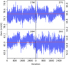 |
Fig. 5. Trace plots of samples of the total gain for randomly selected PIDs for each of the four 30 GHz detectors for our simulation run. The PIDs are, respectively, 349, 9847, 4298, and 1993. The red lines signify the input gain values. |
To validate all scans and detectors, Fig. 6 shows the relative reconstruction bias measured in units of standard deviations, that is:
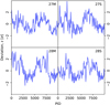 |
Fig. 6. Deviation of the mean output gain solution from the input gain for each PID and 30 GHz detector in our simulation run. The deviations are measured in sample standard deviations. |
where  is the true input total gain,
  is the mean sample total gain estimated over all the samples for a given PID and detector, and σq, i is the sample standard deviation. Thus, the figure shows the deviation of the output gain solution from the input in units of standard deviation. Overall, most samples lies within ±2σ, although there are a few notable outliers. It is also worth noting that the gains are intrinsically correlated in time, and this causes the apparent correlation in this figure.
Finally, in Fig. 7, we show corresponding histograms of the same quantity, but this time aggregated over all PIDs for a given detector. Ideally, these should be Gaussian distributed with zero mean and unit standard deviation. Overall, we see that gain values are generally well-recovered with small biases and reasonable uncertainties. The non-Gaussian features are due to the long correlation lengths seen in Fig. 6, which implies that the number of independent samples in these functions is limited.
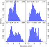 |
Fig. 7. Histograms of the deviations of the mean output gain solution from the input gain, given as the number of sample standard deviations in our simulation run. Each histogram represents the aggregation of the 10 000 PIDs included in the simulation validation. |
5. Results
We are now ready to present gain estimates for each Planck LFI radiometer, as estimated within the end-to-end Bayesian BEYONDPLANCK analysis framework.
5.1. Gain posterior distributions
We start by considering the sampling efficiency of the Monte Carlo chains produced with the above algorithm in terms of mixing and Markov chain correlation lengths. Figure 8 shows total gain as a function of Gibbs iteration for some representative radiometers and PIDs. We see that, overall, the chains are stable and mix well.
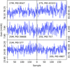 |
Fig. 8. Gibbs chains of the total gain for selected detectors and PIDs. |
A more quantitative confirmation of the good mixing of the chains can be seen in Fig. 9, which shows the correlation lengths across all PIDs (black line is the estimated mean correlation length, whereas the blue bands show the estimated standard deviation). All detectors exhibit correlation coefficients less than 10% after only a few samples.
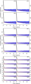 |
Fig. 9. Correlation coefficients as a function of distance between Gibbs samples for 30 (top panel), 44 (middle panel), and 70 GHz (bottom panel) detectors. The black thick line shows the mean value for all PIDs, while the blue band shows the 1σ error bars. |
In Fig. 10, we show relative differences between the last sample of the chain and the first drawn sample (red line) and we compare that to the similar relative difference with the second-to-last sample in the chain (blue line), as well as an in-between chain comparison (green line). We see that even the first sample of the chain is as close to the final solution as the next-to-last sample and the conditional burn-in period with respect to the gain does not significantly affect our results. Long-term burn-in is caused indirectly through correlations with other parameters in the system. Because of these external correlations, we follow BeyondPlanck Collaboration (2023) in omitting the first 200 samples when presenting the final gain estimates.
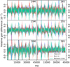 |
Fig. 10. Relative differences between the last sample in one of the BEYONDPLANCK chains and the sample adjacent to the last sample (blue line), the initial sample (the burn-in difference; red line) and the last sample in another chain (green line), for selected detectors. |
In Figs. 11–13, we compare the gain factors derived by BEYONDPLANCK, Planck PR4 and Planck 2018 for each detector. For BEYONDPLANCK, the widths of each curve represent 1σ posterior confidence regions as evaluated directly from the Gibbs chains (after omitting 200 samples for burn-in), while for the other two solutions we only show final best-fit estimates.
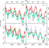 |
Fig. 11. Comparison of gain estimates for the 30 GHz detectors for Planck 2018, Planck PR4, and BEYONDPLANCK. The width of the BEYONDPLANCK line is given by the Monte Carlo uncertainty of the chains. The top x-axis ticks show the date of January 1 of the year marked. |
Overall, the largest differences between BEYONDPLANCK and the other two pipelines are observed in the 30 GHz channel. In particular, we find that the BEYONDPLANCK gain model is systematically lower than the 2018 model by about 0.84% and than PR4 by about 0.67% for this channel, which translates into frequency maps that are about 0.84% (or 0.67%) brighter. We also see that the PR4 and 2018 models agree very well for three of the radiometers, while 28S is an outlier, for which PR4 is close to BEYONDPLANCK.
The 30 GHz channel is the most difficult to calibrate among all three LFI channels because of its brighter foreground signal, and the different ways in which the three pipelines handle this fact makes the above-mentioned gain solution differences less surprising: the PR4 process treats this channel separately, in that this channel is analyzed without priors on polarized foregrounds. The resulting map is then subsequently used as a spatial polarization prior for the 44 and 70 GHz channels (Planck Collaboration Int. LVII 2020). In comparison, the 2018 approach also assumes vanishing CMB polarization during calibration, but this approach make no distinction between the orbital and Solar dipole with respect to absolute gain calibration (as both PR4 and BEYONDPLANCK do), but rather assumes that the fitted foreground model is sufficiently accurate. In contrast, the BEYONDPLANCK pipeline does not treat the 30 GHz channel differently in any way and it also does not assume that the CMB polarization signal vanishes (except for the single quadrupole mode, as discussed in Sect. 2.4). Instead, it uses WMAP information to support the foreground modeling, and to constrain the poorly measured modes in LFI. Overall, these algorithmic differences lead to the observed deviations between the various solutions.
The relative differences are smaller for 44 and 70 GHz: −0.04% (44 GHz) and −0.64% (70 GHz) between BEYONDPLANCK and the Planck 2018 model, and 0.12% (44 GHz) and −0.03% (70 GHz) between BEYONDPLANCK and Planck PR4. There is generally good agreement between the three pipelines for these two channels, although Planck 2018 is generally a higher absolute calibration than for the two others. Differences between BEYONDPLANCK and the two other pipelines are expected due to the joint nature of the BEYONDPLANCK approach and the different ways in which the smoothing of the solutions are performed – BEYONDPLANCK uses the Wiener filter smoothing method, Planck 2018 uses boxcar averaging, and PR4 does not smooth the solution after estimation at all.
5.2. Effects of different gain smoothing approaches on correlated noise stripes
Since the Wiener filtering approach used in this paper has not previously been used for smoothing gain estimates, we compared it with a more conventional boxcar smoothing approach with similar smoothing windows as used by Planck PR4, that is, smoothing windows that dynamically change with the dipole amplitude so as to make the smoothing length shorter in areas of higher signal-to-noise (i.e., dipole maxima).
When comparing the results of these two approaches, we found that with boxcar averaging, the gain solutions behave more like the original Planck 2018 solutions than is the case with Wiener filtering. However, we also found that boxcar smoothing results in correlated noise solutions with strong “stripes” in the binned polarization maps, especially Stokes Q. Reducing the window sizes would mitigate this to some degree (although it introduced other issues, e.g., gain spikes in the low signal-to-noise regime) and we therefore find it likely that the correlated noise stripes are related to an “oversmoothing” of the gain solution.
With the Wiener filter process, we are, modulo the exact form of the prior covariance matrix, smoothing the data in an optimal way – in high signal-to-noise areas, the signal is allowed to determine the solution and in low signal-to-noise areas, the prior ensures that the solution does not become nonphysical. In Fig. 14, we show a comparison of the effect of these two approaches on the Stokes Q map. In this figure, the only difference in the underlying sampling algorithm is the choice of boxcar smoothing and Wiener filtering. Thus, it is reassuring to find that Wiener filtering (in line with the expectations) is apparently able to find smooth gain solutions that avoid the problem of oversmoothing.
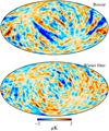 |
Fig. 14. Random Gibbs sample of the map of the correlated noise, ncorr, of the Q Stokes parameter for the 44 GHz frequency channel, smoothed to an effective angular resolution of 5° FWHM. The top figure is the map resulting from a boxcar smoothed gain solution, whereas the bottom figure is the map which results from smoothing the gain solution with a Wiener filter. |
5.3. Gain jumps
As noted from the beginning of the Planck experiment (see, e.g., Planck Collaboration XXVIII 2014), the physical gain of the instrument exhibits several sharp jumps. These jumps are related to changes in the thermal environment of the instrument – an example of such an event is the turning off of the 20 K sorption cooler. Not all of the events are well understood and can mainly be traced after an initial gain estimation.
Such jumps must be accounted for in any gain estimation approach that isn’t purely data-driven; namely, if we are applying priors in any way that set up expected correlated behaviors between the gain factors over the mission. We find that indeed the Wiener filter approach is able to account for such jumps without any extra hard-coding (see Fig. 15, where a Wiener filter solution applied globally to the whole PID range is shown along with two jumps), another advantage of this smoothing method compared to the boxcar approach, where such jumps must be specified in the code and explicitly excluded from the averaging.
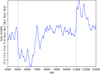 |
Fig. 15. Examples of jumps seen in the gain factors. The line shows the Wiener filter solution for the 27M detector, while the vertical lines show the locations of the jumps. The jump at around PID 11000 is the sorption cooler switch-over event, mentioned in Sect. 5.3. |
5.4. Comparison with external data
To understand the combined impact of the various gain model differences discussed above, it is useful to compare the final BEYONDPLANCK frequency maps with externally processed observations, both from WMAP and Planck. In this respect, we note that both the Planck 2018 and WMAP data sets are associated with sets of correction templates that track known systematic effects (or poorly measured modes) in the respective sky maps. For the Planck 2018 30 GHz channel, this template is shown in Fig. 16. As discussed by Planck Collaboration II (2020), this template was produced by iterating between calibration and component separation and it therefore traces uncertainties in the gain model due to foreground uncertainties. Furthermore, due to limited time, only four full iterations of this type were completed for the Planck 2018 analysis and we must therefore expect that there are still residuals of this type present in the final sky maps at some level.
 |
Fig. 16. Gain residual template for the LFI 30 GHz channel, produced in the Planck 2018 analysis through manual iteration between calibration, mapmaking and component separation (Planck Collaboration II 2020). |
With this in mind, we show in Fig. 17 BEYONDPLANCK–PR4 and BEYONDPLANCK–Planck 2018 difference maps for Stokes I, Q, and U (columns), for all three LFI frequencies (rows). The first, third, and fifth rows show differences with respect to Planck 2018, while the second, fourth, and sixth rows show differences with respect to PR4. Several features in these difference maps are interesting from the calibration perspective. Starting with the PR4 temperature difference maps, we see that all three channels are dominated by a clean dipole-like residual aligned with the Solar CMB dipole. This shows that the BEYONDPLANCK and PR4 temperature maps are morphologically very similar, but have different absolute calibration. We also see that the temperature map difference between BEYONDPLANCK and PR4 exhibits a flip in the dipole direction going from 30 and 44 to 70 GHz. This sign change is consistent with the differences in the calibration factors between 44 and 70 GHz reported in Table 10 in Planck Collaboration Int. LVII (2020), finding a difference of 0.31% between the absolute calibration of the 44 and 70 GHz channels. Since the CMB Solar dipole has an amplitude of about 3360 μK, this relative difference translates into an absolute temperature difference of roughly 10 μK in the observed sky signal, which is fully consistent with the dipole differences we see in Fig. 17. In comparison, the Planck 2018 versus BP difference maps in temperature (lines 1, 3, and 5) show a more prominent quadrupolar structure with a morphology that might resemble the effect of bandpass mismatch leakage (Planck Collaboration X 2016; Planck Collaboration Int. LVII 2020).
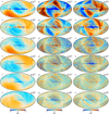 |
Fig. 17. Differences between BEYONDPLANCK and Planck 2018 or Planck PR4 frequency maps, smoothed to a common angular resolution of 2° FWHM. Columns show Stokes T, Q, and U parameters, respectively, while rows show pairwise differences with respect to the pipeline indicated in the panel labels. A constant offset has been removed from the temperature maps, while all other modes are retained. The 2018 maps have been scaled by their respective beam normalization prior to subtraction. Reproduced from Basyrov et al. (2023). |
For the polarization, the most striking differences are seen in the 30 GHz channel, for which variations at the 4 μK level are seen over large fractions of the sky. Furthermore, these residuals correlated very closely with the Planck 2018 gain template shown in Fig. 16, suggesting that they are indeed caused by foreground-induced gain residuals. The same patterns are also seen in the PR4 difference maps, but with a notably lower level.
For the 44 GHz maps, we note that the Stokes Q difference maps show correlated noise stripes similar to those highlighted in the top figure in Fig. 14. However, we also note that these structures have different amplitudes in Planck PR4 and Planck 2018, and these stripes are therefore present in at least one of the other pipelines as well, and possibly both.
Figure 18 shows a similar comparison between the various Planck 30 GHz maps and the WMAP K-band channel (Bennett et al. 2013). In this case, all maps have been smoothed to a common angular resolution of 3° FWHM, and the K-band map has been scaled by a factor of 0.495 to account for the different center frequencies of the two maps while adopting a synchrotron-like spectral index of βs = −3.1. From top to bottom, the first three rows show difference maps with respect to Planck 2018, Planck PR4, and BEYONDPLANCK. Such a differencing removes the expected synchrotron contribution, and assuming the standard results for polarized microwave emission hold (i.e., that there so far have been no measurements of polarized spinning dust), only CMB and instrumental effects should remain.
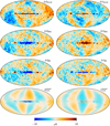 |
Fig. 18. Difference maps between the Planck 30 GHz and WMAP K-band maps for Planck 2018 (first row), Planck PR4 (second row), and BEYONDPLANCK (third row). All maps have been smoothed to a common angular resolution of 3° FWHM before evaluating the differences. The WMAP K-band map has been scaled by a factor of 0.495 to account for different center frequencies, assuming a synchrotron spectral index of βs = −3.1. Bottom row shows one of the WMAP K-band transmission imbalance templates discussed by Jarosik et al. (2007), which accounts for known poorly measured modes in the WMAP data. |
Overall, we see a clear progression in agreement with respect to WMAP K-band, in the sense that BEYONDPLANCK shows smaller residuals than Planck PR4; this, in turn, shows smaller residuals than Planck 2018. Furthermore, we note that the strong residuals traced by the LFI gain template in Fig. 16 are most pronounced in the Planck 2018 map.
At the same time, we also observe significant coherent large-scale features in the difference map between BEYONDPLANCK and K-band. To at least partially understand these, we show the WMAP transmission imbalance templates derived by Jarosik et al. (2007) in the bottom row of Fig. 17. These templates trace poorly measured modes due to the differential nature of the WMAP instrument. Although corrections for this effect are applied to the final K-band sky maps, the uncertainty on the template amplitudes is estimated to 20%. Considering the tight correlation between the BEYONDPLANCK–WMAP difference map and the transmission imbalance template, it seems clear that at least a significant fraction of the remaining residual may be explained in terms of this effect. Of course, this also suggests that a future joint analysis between Planck and WMAP in time-domain will be able to constrain the WMAP transmission imbalance parameters to much higher precision, and Planck data can thereby be used to break an important internal degeneracy in WMAP. As reported by Watts et al. (2023), this work has already started, but a full exploration of time-ordered WMAP data is outside the scope of the current analysis. We also emphasize that the current BEYONDPLANCK analysis only uses low-resolution WMAP polarization data for which a full covariance matrix is available and these modes are appropriately down-weighted in those matrices.
6. Conclusions
Here, we present the BEYONDPLANCK approach to gain calibration within the larger Commander Gibbs sampling framework. This framework relies directly on the Solar and orbital dipoles for relative and absolute calibration, respectively, and accounts for astrophysical foreground and instrumental systematics through global modeling.
One critically important difference with respect to previous Planck LFI analysis efforts is the fact that we actively use external data to break internal Planck degeneracies and, in particular, WMAP observations. This significantly alleviates the need for imposing strong algorithmic priors during the calibration process. Most notably, while both the Planck 2018 and Planck PR4 pipelines have assumed CMB polarization to be negligible on all angular scales during the calibration phase, we can only assume that the CMB quadrupole is negligible. The reason we still make this assumption is that the Planck scanning strategy renders the CMB quadrupole very nearly perfectly degenerate with the CMB Solar dipole coupled to subtle gain fluctuations; a hypothetical future and well-designed satellite mission should not require this prior, as long as its scanning strategy modulates the CMB dipole on sufficiently short time-scales and with good cross-linking.
Overall, we find good agreement between the BEYONDPLANCK and previous gain models. The biggest differences are observed in the LFI 30 GHz channel, with gain variations of 0.84% between Planck 2018 and BEYONDPLANCK. These differences result in subtle but significant temperature and polarization residuals. When comparing these with external WMAP K-band observations, it appears clear that the BEYONDPLANCK LFI maps are generally cleaner than previous renditions with respect to gain residuals. At the same time, we emphasize that these differences are also consistent with previously published error estimates, as presented by the Planck 2018 and Planck PR4 teams themselves. For instance, the morphology of the Planck 2018 polarization residuals matches previously published LFI DPC gain residual templates (Planck Collaboration II 2020), and the PR4 absolute calibration differences are fully consistent with internal PR4 estimates (Planck Collaboration Int. LVII 2020). These results are thus neither novel nor surprising, but they simply highlight the inherent advantages of global analysis, using complementary data sets to break internal degeneracies.
Finally, we note that even though the procedures outlined in this paper have been aimed at modeling the LFI detectors, there is nothing about the data model or methodology that is unique with regard to LFI. The method should be directly applicable for other data sets and experiments as well, and, indeed, a preliminary WMAP analysis is already underway (Watts et al. 2023).
Here, a “sample” means the detector readout at every 1/fsamp seconds, where fsamp is the sampling frequency of the instrument. The whole set of these samples is called the time-ordered data (TOD). The sampling frequency for the three LFI instruments are 32.5 Hz, 46.5 Hz, and 78.8 Hz for the 30 GHz, 44 GHz, and 70 GHz instrument, respectively.
The scanning strategy adopted by Planck means that the time interval between successive measurements of the same point on the sky with the same detector from a different angle can be as much as six months (if the point lies along the ecliptic). During this time, several environmental parameters of the detector may have changed.
Although not shown here, sampling from P(g ∣ stot, ncorr, d, …) would follow the exact same procedure, but with a noise covariance matrix given by Nwn instead of Nwn + Ncorr. Nwn is a diagonal matrix, while Ncorr is not, and since most operations are less heavy, computationally speaking, when diagonal matrices are involved, the resulting sampling process would also be lighter in that case.
Note that we do not apply any priors on g0 in this paper, which corresponds to S−1 = 0, adopting the notation of BeyondPlanck Collaboration (2023), where S is the prior covariance of g0. The remaining notational differences between Eqs. (17) and (A.10) in that paper arise from our organizing all vectors and matrices in terms of independent detectors, using the fact that ntot is assumed to be independent between detectors; this may not be strictly true in practice, as discussed by Ihle et al. (2023), and future analyses may prefer to account for the full joint matrix.
Acknowledgments
We thank Prof. Pedro Ferreira and Dr. Charles Lawrence for useful suggestions, comments and discussions. We also thank the entire Planck and WMAP teams for invaluable support and discussions, and for their dedicated efforts through several decades without which this work would not be possible. The current work has received funding from the European Union’s Horizon 2020 research and innovation programme under grant agreement numbers 776282 (COMPET-4; BEYONDPLANCK), 772253 (ERC; BITS2COSMOLOGY), and 819478 (ERC; COSMOGLOBE). In addition, the collaboration acknowledges support from ESA; ASI and INAF (Italy); NASA and DoE (USA); Tekes, Academy of Finland (grant no. 295113), CSC, and Magnus Ehrnrooth foundation (Finland); RCN (Norway; grant nos. 263011, 274990); and PRACE (EU).
References
- Basyrov, A., Suur-Uski, A.-S., Colombo, L. P. L., et al. 2023, A&A, 675, A10 (BeyondPlanck SI) [NASA ADS] [CrossRef] [EDP Sciences] [Google Scholar]
- Bennett, C. L., Larson, D., Weiland, J. L., et al. 2013, ApJS, 208, 20 [Google Scholar]
- BeyondPlanck Collaboration (Andersen, K. J., et al.) 2023, A&A, 675, A1 (BeyondPlanck SI) [Google Scholar]
- Brilenkov, M., Fornazier, K. S. F., Hergt, L. T., et al. 2023, A&A, 675, A4 (BeyondPlanck SI) [NASA ADS] [CrossRef] [EDP Sciences] [Google Scholar]
- de Bernardis, P., Ade, P. A. R., Bock, J. J., et al. 2000, Nature, 404, 955 [Google Scholar]
- Delouis, J. M., Pagano, L., Mottet, S., Puget, J. L., & Vibert, L. 2019, A&A, 629, A38 [NASA ADS] [CrossRef] [EDP Sciences] [Google Scholar]
- Fixsen, D. J. 2009, ApJ, 707, 916 [Google Scholar]
- Godard, B., Croon, M., Budnik, F., & Morley, T. 2009, Proceedings of the 21st International Symposium on Space Flight Dynamics (ISSFD), Toulouse [Google Scholar]
- Greason, M. R., Limon, M., Wollack, E., et al. 2012, Nine-Year Explanatory Supplement, 5th edn. (Greenbelt: NASA/GSFC) [Google Scholar]
- Hinshaw, G., Weiland, J. L., Hill, R. S., et al. 2009, ApJS, 180, 225 [Google Scholar]
- Ihle, H. T., Bersanelli, M., Franceschet, C., et al. 2023, A&A, 675, A6 (BeyondPlanck SI) [NASA ADS] [CrossRef] [EDP Sciences] [Google Scholar]
- Jarosik, N., Barnes, C., Greason, M. R., et al. 2007, ApJS, 170, 263 [NASA ADS] [CrossRef] [Google Scholar]
- Kogut, A., Fixsen, D. J., Chuss, D. T., et al. 2011, J. Cosmol. Astropart. Phys., 2011, 025 [CrossRef] [Google Scholar]
- Kovac, J. M., Leitch, E. M., Pryke, C., et al. 2002, Nature, 420, 772 [NASA ADS] [CrossRef] [Google Scholar]
- Planck Collaboration I. 2011, A&A, 536, A1 [NASA ADS] [CrossRef] [EDP Sciences] [Google Scholar]
- Planck Collaboration II. 2014, A&A, 571, A2 [NASA ADS] [CrossRef] [EDP Sciences] [Google Scholar]
- Planck Collaboration VIII. 2014, A&A, 571, A8 [NASA ADS] [CrossRef] [EDP Sciences] [Google Scholar]
- Planck Collaboration XXVIII. 2014, A&A, 571, A28 [NASA ADS] [CrossRef] [EDP Sciences] [Google Scholar]
- Planck Collaboration II. 2016, A&A, 594, A2 [NASA ADS] [CrossRef] [EDP Sciences] [Google Scholar]
- Planck Collaboration V. 2016, A&A, 594, A5 [NASA ADS] [CrossRef] [EDP Sciences] [Google Scholar]
- Planck Collaboration VIII. 2016, A&A, 594, A8 [NASA ADS] [CrossRef] [EDP Sciences] [Google Scholar]
- Planck Collaboration X. 2016, A&A, 594, A10 [NASA ADS] [CrossRef] [EDP Sciences] [Google Scholar]
- Planck Collaboration I. 2020, A&A, 641, A1 [NASA ADS] [CrossRef] [EDP Sciences] [Google Scholar]
- Planck Collaboration II. 2020, A&A, 641, A2 [NASA ADS] [CrossRef] [EDP Sciences] [Google Scholar]
- Planck Collaboration III. 2020, A&A, 641, A3 [NASA ADS] [CrossRef] [EDP Sciences] [Google Scholar]
- Planck Collaboration IV. 2020, A&A, 641, A4 [NASA ADS] [CrossRef] [EDP Sciences] [Google Scholar]
- Planck Collaboration Int. XLVI. 2016, A&A, 596, A107 [NASA ADS] [CrossRef] [EDP Sciences] [Google Scholar]
- Planck Collaboration Int. LVII. 2020, A&A, 643, A42 [NASA ADS] [CrossRef] [EDP Sciences] [Google Scholar]
- Smoot, G. F., Bennett, C. L., Kogut, A., et al. 1992, ApJ, 396, L1 [Google Scholar]
- Watts, D. J., Galloway, M., Ihle, H. T., et al. 2023, A&A, 675, A16 (BeyondPlanck SI) [NASA ADS] [CrossRef] [EDP Sciences] [Google Scholar]
All Figures
|
Fig. 1. Comparison of different contributions to the time-ordered data seen by Planck at 30 GHz, for a PID whose spin orientation is close to perpendicular to the dipole axis. The blue and black curves show the orbital and Solar CMB dipoles, respectively. The red and grey lines show the Solar CMB dipole with galactic foregrounds and instrumental noise added, respectively. |
| In the text | |
|
Fig. 2. Comparison of the CMB temperature dipole (thick black line) observed through the Planck scanning strategy with three random polarization quadrupole simulations (thin colored lines); the latter have been scaled by a factor of 104 for visualization purposes. |
| In the text | |
|
Fig. 3. Correlated noise maps for the 30 GHz channel in a Gibbs chain that includes (left panel) or neglects (right panel) gain time-dependencies. All maps are smoothed to a common resolution of 2.5° FWHM. |
| In the text | |
|
Fig. 4. Processing masks used in gain and correlated noise estimation for each frequency channel. The allowed 30 GHz sky fraction (blue) is 0.73, the 44 GHz sky fraction (green) is 0.81, and the 70 GHz sky fraction (red) is 0.77. |
| In the text | |
|
Fig. 5. Trace plots of samples of the total gain for randomly selected PIDs for each of the four 30 GHz detectors for our simulation run. The PIDs are, respectively, 349, 9847, 4298, and 1993. The red lines signify the input gain values. |
| In the text | |
|
Fig. 6. Deviation of the mean output gain solution from the input gain for each PID and 30 GHz detector in our simulation run. The deviations are measured in sample standard deviations. |
| In the text | |
|
Fig. 7. Histograms of the deviations of the mean output gain solution from the input gain, given as the number of sample standard deviations in our simulation run. Each histogram represents the aggregation of the 10 000 PIDs included in the simulation validation. |
| In the text | |
|
Fig. 8. Gibbs chains of the total gain for selected detectors and PIDs. |
| In the text | |
|
Fig. 9. Correlation coefficients as a function of distance between Gibbs samples for 30 (top panel), 44 (middle panel), and 70 GHz (bottom panel) detectors. The black thick line shows the mean value for all PIDs, while the blue band shows the 1σ error bars. |
| In the text | |
|
Fig. 10. Relative differences between the last sample in one of the BEYONDPLANCK chains and the sample adjacent to the last sample (blue line), the initial sample (the burn-in difference; red line) and the last sample in another chain (green line), for selected detectors. |
| In the text | |
|
Fig. 11. Comparison of gain estimates for the 30 GHz detectors for Planck 2018, Planck PR4, and BEYONDPLANCK. The width of the BEYONDPLANCK line is given by the Monte Carlo uncertainty of the chains. The top x-axis ticks show the date of January 1 of the year marked. |
| In the text | |
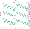 |
Fig. 12. Comparison of gain estimates for the 44 GHz detectors. See Fig. 11 for details. |
| In the text | |
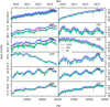 |
Fig. 13. Comparison of gain estimates for the 70 GHz detectors. See Fig. 11 for details. |
| In the text | |
|
Fig. 14. Random Gibbs sample of the map of the correlated noise, ncorr, of the Q Stokes parameter for the 44 GHz frequency channel, smoothed to an effective angular resolution of 5° FWHM. The top figure is the map resulting from a boxcar smoothed gain solution, whereas the bottom figure is the map which results from smoothing the gain solution with a Wiener filter. |
| In the text | |
|
Fig. 15. Examples of jumps seen in the gain factors. The line shows the Wiener filter solution for the 27M detector, while the vertical lines show the locations of the jumps. The jump at around PID 11000 is the sorption cooler switch-over event, mentioned in Sect. 5.3. |
| In the text | |
|
Fig. 16. Gain residual template for the LFI 30 GHz channel, produced in the Planck 2018 analysis through manual iteration between calibration, mapmaking and component separation (Planck Collaboration II 2020). |
| In the text | |
|
Fig. 17. Differences between BEYONDPLANCK and Planck 2018 or Planck PR4 frequency maps, smoothed to a common angular resolution of 2° FWHM. Columns show Stokes T, Q, and U parameters, respectively, while rows show pairwise differences with respect to the pipeline indicated in the panel labels. A constant offset has been removed from the temperature maps, while all other modes are retained. The 2018 maps have been scaled by their respective beam normalization prior to subtraction. Reproduced from Basyrov et al. (2023). |
| In the text | |
|
Fig. 18. Difference maps between the Planck 30 GHz and WMAP K-band maps for Planck 2018 (first row), Planck PR4 (second row), and BEYONDPLANCK (third row). All maps have been smoothed to a common angular resolution of 3° FWHM before evaluating the differences. The WMAP K-band map has been scaled by a factor of 0.495 to account for different center frequencies, assuming a synchrotron spectral index of βs = −3.1. Bottom row shows one of the WMAP K-band transmission imbalance templates discussed by Jarosik et al. (2007), which accounts for known poorly measured modes in the WMAP data. |
| In the text | |
Current usage metrics show cumulative count of Article Views (full-text article views including HTML views, PDF and ePub downloads, according to the available data) and Abstracts Views on Vision4Press platform.
Data correspond to usage on the plateform after 2015. The current usage metrics is available 48-96 hours after online publication and is updated daily on week days.
Initial download of the metrics may take a while.