


| Issue |
A&A
Volume 711, July 2026
|
|
|---|---|---|
| Article Number | A242 | |
| Number of page(s) | 20 | |
| Section | Extragalactic astronomy | |
| DOI | https://doi.org/10.1051/0004-6361/202557020 | |
| Published online | 24 July 2026 | |
X-ray view of a massive node of the cosmic web at z ∼ 3
II. Discovery of extended X-ray emission around a hyperluminous quasar
1
Dipartimento di Fisica “G. Occhialini”, Università degli Studi di Milano-Bicocca, Piazza della Scienza 3, I-20126 Milano, Italy
2
Kapteyn Astronomical Institute, University of Groningen, Landleven 12, 9747, AD, Groningen, The Netherlands
3
INAF – Osservatorio Astrofisico di Arcetri, Largo E. Fermi 5, 50127 Firenze, Italy
4
Université Côte d’Azur, Observatoire de la Côte d’Azur, CNRS, Laboratoire Lagrange, France
5
Dipartimento di Fisica – Sezione di Astronomia, Università di Trieste, Via Tiepolo 11, 34131 Trieste, Italy
6
IFPU, Institute for Fundamental Physics of the Universe, Via Beirut 2, 34151 Trieste, Italy
7
INAF – Osservatorio Astronomico di Trieste, Via G. B. Tiepolo 11, 34143 Trieste, Italy
8
INFN, Sezione di Trieste, Via Valerio 2, 34127 Trieste, Italy
9
Université Paris-Saclay, Université Paris Cité, CEA, CNRS, AIM, 91191 Gif-sur-Yvette, France
10
Harvard-Smithsonian Center for Astrophysics, 60 Garden St., Cambridge, MA 02138, USA
11
INAF – Osservatorio Astronomico di Roma, Via Frascati 33, 00040 Monte Porzio Catone, Rome, Italy
12
Space Science Data Center, Agenzia Spaziale Italiana, Via del Politecnico snc, 135, Roma, Italy
13
INAF – Osservatorio di Astrofisica e Scienza dello Spazio di Bologna, Via Piero Gobetti 93/3, 40129 Bologna, Italy
★ Corresponding author: This email address is being protected from spambots. You need JavaScript enabled to view it.
Received:
28
August
2025
Accepted:
27
May
2026
Abstract
While the warm (T ∼ 104 K), ionized gas in the circumgalactic medium (CGM) at z > 3 is now routinely observed around bright quasars in Lyα emission, little is known about the CGM hot phase (T ∼ 107 K). Here, we report the analysis of 634 ks of Chandra X-ray observations in the MQN01 Cosmic Structure, a region containing one of the brightest Lyα nebulae and the largest galaxy overdensity known at z > 3. We detect ≈66 net counts (≈8σ) of X-ray emission in the 0.5–2 keV band extending to at least ∼30 kpc from the brightest quasar in MQN01. The morphology and spectrum are consistent with thermal emission from hot plasma in collisional ionization equilibrium. Quasi-stellar object (QSO) photoionization is found to have a negligible impact, and alternative scenarios such as inverse Compton scattering are disfavoured. A joint spatial and spectral Markov chain Monte Carlo (MCMC) analysis provides consistency with a β model with a steep density profile (β ≃ 2.0+1.4−0.8, rcore = 36+13−16 kpc) and an average gas temperature of kT ≃ (1.8 ± 0.4) keV. Assuming that the QSO resides within a virialized halo, whose virial temperature is equal to the observed gas temperature, the implied halo mass and virial radius would be Mvir ∼ 3 × 10¹³ M⊙ and ∼190 kpc. Further assuming that the observed emission traces the brighter inner region of a distribution extending to the virial radius, the extrapolated hot gas mass would be Mhot ≈ 2.6+1.7−0.6 × 10¹² M⊙, which is ≃ 8.3+3.0−9.8% of Mvir, or 56+65−20% of the theoretical cosmological baryon budget of the halo. The hot gas also emits an exceptionally high X-ray luminosity, with a measured L2 − 10 = 2.25−1.38+0.77 × 1045 erg s−1 within the central 30 kpc. This system is a clear outlier in the LX–TX plane, indicating a thermodynamic state distinct from that of evolved lower-redshift hot halos. The cooling time in the inner 15-30 kpc is comparable to the local dynamical time (1 < tcool/tff < 10), suggesting that the gas could become locally unstable in the absence of heating or feedback. Moreover, the thermal pressure associated with the detected CGM hot phase is large enough to confine the cold and dense clumps, which are required to reproduce the high Lyα emission associated with the inner regions of the MQN01 structure. Although limited to a single system, our results provide unique information on the multi-phase properties of the CGM (or proto-intracluster medium) and a view of the nascent thermal hot gas phase observed in local galaxy clusters.
Key words: radiation mechanisms: thermal / galaxies: clusters: intracluster medium / galaxies: halos / intergalactic medium / quasars: supermassive black holes
© The Authors 2026
 Open Access article, published by EDP Sciences, under the terms of the Creative Commons Attribution License (https://creativecommons.org/licenses/by/4.0), which permits unrestricted use, distribution, and reproduction in any medium, provided the original work is properly cited.
This article is published in open access under the Subscribe to Open model. This email address is being protected from spambots. You need JavaScript enabled to view it. to support open access publication.
1. Introduction
Galaxy clusters host the largest reservoirs of hot gas known as the intracluster medium (ICM), which is prominently observed through X-ray emission. According to the hierarchical structure formation paradigm, these massive systems form through the gravitational collapse and merging of smaller structures (Peebles 1980; Navarro et al. 1996). Gas infalling into the cluster potential well undergoes shock heating, reaching temperatures of ∼107 − 108 K (Rosati et al. 2002; Kravtsov & Borgani 2012). The dominant X-ray emission mechanism of the ICM is thermal bremsstrahlung, producing luminosities from LX ∼ 1043 to more than 1045 erg s−1.
At higher redshifts (2 < z < 3), massive halos are expected to host a nascent hot circumgalactic medium (CGM) or proto-ICM, influenced by both gravitational processes and non-gravitational effects such as active galactic nucleus (AGN) and supernova feedback, although the formation scenario is still unclear (Shimakawa et al. 2018; Kooistra et al. 2022). Detecting extended X-ray emission from these structures is particularly challenging due to instrumental sensitivity limits and the need for a high angular resolution to separate diffuse emission from point sources. This is crucial at z > 2, where massive halos often host a central AGN that can dominate the X-ray signal. Models and simulations predict that the X-ray emission from hot gas at z > 2 is faint and spatially compact, with an extent on the order of a few tens of arcseconds (i.e. approximately tens of kiloparsecs; Saro et al. 2009). Therefore, observations require not only a high sensitivity but also a high angular resolution, a capability currently achieved only by the Chandra X-ray telescope (on-axis angular resolution at energies of ∼1.5 keV is 0.8″, half-power diameter1) and the ability to perform spatially resolved spectral analysis. Therefore, Chandra’s capabilities are unparalleled for studying extended X-ray emission on scales from kiloparsecs to a few megaparsecs, particularly in high-z systems. Constraining the thermal properties of the hot CGM at these early epochs is essential for testing models of the redshift evolution of galaxy halos, such as the transition between cold and hot accretion modes (e.g. Dekel & Birnboim 2006), and for understanding the role of feedback in shaping the thermodynamic state of diffuse gas in forming clusters.
The most distant potential X-ray detection of thermal emission from the ICM associated with a relaxed galaxy cluster has been reported in a system at z ∼ 2.5 by Wang et al. (2016). A robust detection of thermal ICM emission was observed in the galaxy cluster XLSSC122 at z ≃ 2 by van Marrewijk et al. (2024). At redshifts of z > 3, most of the extended X-ray emission has been found around radio-loud galaxies (Yuan et al. 2003; Smail et al. 2012), and is thus associated with non-thermal emission from inverse Compton (IC) scattering of cosmic microwave background (CMB) photons by relativistic electrons in radio jets, as confirmed by the X-ray hard spectrum and the overlap with the radio jets. Recently, Tozzi et al. (2022) and Lepore et al. (2024) (hereafter L24) have reported direct evidence of the proto-ICM at high redshift, presenting a detailed analysis of the extended thermal X-ray emission within 150 kpc of a radio galaxy in the Spiderweb protocluster at z = 2.156. After accounting for non-thermal IC emission from the radio jet, they identified diffuse thermal emission from hot (kT ∼ 2 keV) gas with a mass of ∼ 1.6 × 10¹² M⊙, within a halo whose total mass is estimated to be ∼ 0.6−1.4 × 10¹³ M⊙. The combination of X-ray and Sunyaev-Zeldovich (SZ; Di Mascolo et al. 2023) detections revealed an entropy profile indicative of a cool-core system, with a cooling time of fewer than 100 Myr and a potential mass deposition rate of 250–1000 M⊙ yr−1, consistent with infrared-based star formation rates of the central galaxy. These results suggest that AGN feedback and cooling flows may coexist in the early stages of protocluster formation.
This work is the second in a series of papers investigating deep (634 ks) Chandra X-ray observations of a protocluster at z = 3.25, centred on the luminous quasi-stellar object (QSO) CTS G18.01 (hereafter ID1; see Travascio et al. 2025). This QSO lies at the centre of the Multi Unit Spectroscopic Explorer (MUSE) Quasar Nebula 01 (MQN01), a giant (> 200 kpc) Lyα nebula in the sample of Borisova et al. (2016). Recent observations, based on a mosaic of eight VLT/MUSE AO-WFM pointings, have further extended its detection beyond two arcminutes (Cantalupo et al., in prep.). To investigate the connection between the properties of this cosmic web node and its galaxy population, multi-wavelength campaigns are actively characterizing the protocluster members (Pensabene et al. 2024; Galbiati et al. 2025). In our previous paper, we conducted a census of X-ray AGNs embedded in the protocluster, identifying six AGNs within an area of ≈16 cMpc2 and a velocity range of ±1000 km s−1 from the redshift of the central ID1. This corresponds to a significant overdensity of log(L2−10 keV/ers s−1) > 43 X-ray AGNs relative to the X-ray AGN space density in the field as constrained by Gilli et al. (2007).
In this second paper, based on the same Chandra X-ray dataset, we focus on the extended X-ray emission around the luminous QSO ID1. In Section 2, we describe the Chandra data reduction and astrometric correction, respectively. In Section 3.1, we report a significant detection of spatially resolved X-ray emission at observed energies below 2 keV, extending out to at least 30 kpc from the QSO. Section 3.2 examines the morphology of this emission in comparison with the Lyα nebula previously identified around the same QSO by Borisova et al. (2016), while Section 3.3 presents an analysis of its spectral properties. In Section 4, we investigate the physical properties of the hot gas under the assumption of a thermal origin. Discussions about the potential influence of QSO photoionization on the thermal emission and alternative emission mechanisms are presented in Sections 5.1 and 5.2. Finally, in Sections 5.4 and 5.6, we compare the properties of this system with those of the hot halo in the Spiderweb protocluster, with predictions from numerical simulations, and with observations of local galaxy clusters and groups.
Throughout this paper, all energies are reported in the observed frame unless stated otherwise, with fluxes consistently referring to observed energy bands. In contrast, luminosities are given in rest-frame energy bands. We adopt the same cosmological model as Travascio et al. (2025)2, in which 1″ corresponds to 7.663 physical kpc. In Section 4, we assume a cosmic baryonic fraction of fb = Ωb/Ωm = 0.15 to evaluate the reliability of our best-fit model. Unless otherwise noted, all uncertainties shown in the plots correspond to the 1σ (68%) confidence level.
2. Methods
2.1. Chandra observations and data reduction
For this study, we used X-ray observations taken with the Chandra Advanced CCD Imaging Spectrometer (ACIS-I) during Cycle 23 (2022/2023), with a total exposure time of 634 ks (PI: S. Cantalupo; see Travascio et al. 2025 for further details). These observations were conducted in Very Faint (VFAINT) mode, which optimizes the separation of good and bad X-ray events by using the 5 × 5 pixel event island to improve event classification. We performed the data reduction using CIAO 4.17 and the Chandra Calibration Database (CALDB 4.12.2) installed on Python 3.10. We removed flares identified in the light curves and corrected the astrometry of each ObsID according to the co-ordinates of the brightest QSO extracted in the GAIA catalogue.
2.2. Refined astrometric alignment of ObsIDs
In Travascio et al. (2025), the different ObsIDs were aligned by cross-matching the positions of bright, point-like sources and estimating the least-squares minimization to determine the optimal transformation relative to the deepest ObsID. This is the best method to produce a catalogue of X-ray sources in a wide field. However, in this paper, our main purpose is to explore the presence of extended X-ray emission around the AGNs identified in Travascio et al. (2025). This aim requires a more refined astrometric alignment, made ad hoc for the individual X-ray sources, minimizing positional uncertainties and ensuring that any observed extended emission is not an artifact of residual misalignment. However, this approach is feasible only for QSO ID1, which has enough photon counts in each ObsID to reliably determine the centroid position. For the other AGNs, multi-source alignment remains the most suitable option. More specifically, for QSO ID1, the 0.5–2 keV image of each ObsID was re-binned to one-fourth of the native pixel size and smoothed with a Gaussian kernel of 3 sub-pixels. The position of the QSO ID1 in each image was determined by computing the centroid’s co-ordinates within a 2″-radius circular region, centred on the approximate location of the QSO. Using the wcs_match tool, we generated a translation matrix for all ObsIDs, with the deepest ObsID used as the reference. We then applied this transformation to reproject the event and aspect files using the wcs_update tool. Figure A.1 in Appendix A shows the results of this alignment, displaying the 0.5–2 keV images of the ObsIDs after re-binning and Gaussian smoothing. We then generated a new merged event file by combining the aligned ObsIDs.
3. Results
3.1. Detection and validation of extended X-ray emission around the hyperluminous QSO ID1
We investigated the presence of extended X-ray emission around the six X-ray-detected AGNs in the MQN01 protocluster (Travascio et al. 2025). For this purpose, we compared the observed emission with the expected point spread function (PSF), considering different energy bands. At the position of each AGN and in each selected energy band, we simulated 500 individual PSFs predicted in each ObsID in our dataset. To generate these 500 simulated PSFs, we used the simulate_psf tool3 in CIAO, which accounts for the instrument’s response and observational conditions associated with each ObsID. The ACIS readout streak has not been included in the PSF simulations. A simple estimate of the streak brightness shows that its effect is negligible for our findings. We also verified that the pile-up effect is negligible for the observed count rate.
This method requires a spectral model for the energy band of interest. Therefore, we extracted a spectrum within a 2″ radius for each AGN, as this radius contains more than 98% of the PSF photons, independent of the spectral model. For each source and energy band, the composite PSF was constructed by weighting each simulated PSF by the exposure time of the corresponding ObsID and summing them.
After generating the PSF images, we compared their radial surface count profiles with those extracted from the observations. We estimated the radial surface count profile of the central AGN and subtracted the background level, determined from the outermost radial bins. For a consistent comparison with the PSF profile, we normalized the simulated PSF by scaling its total counts within a 2″ radius to match the corresponding counts in the observed, background-subtracted count profile centred on the QSO. To mitigate the uncertainties about the PSF centring, we aligned the PSF peak with the centroid of the observed X-ray emission and re-projected the PSF onto the same pixel grid using first-order interpolation. Finally, we quantified any residual excess emission in terms of σ by subtracting the expected (PSF+background) counts from the observed counts in each radial bin and dividing by the combined uncertainty, which includes both statistical (Poisson) errors and background estimation uncertainties.
Our analysis reveals a significant extended X-ray emission associated with only one AGN in MQN01, the QSO ID1, in the soft X-ray regime (0.5–2 keV observed, corresponding to ∼2–8.5 keV rest-frame at z = 3.2502). The left and middle panels in Figure 1 display the radial profiles and residuals for ID1 in the 0.5–2.0 keV and 2.0–10.0 keV energy bands, respectively, extending out to ∼12″ (≈ 90 kpc), and by masking the nearest X-ray neighbours of the QSO, which are ID3 and ID4 in Travascio et al. (2025). The radial bins were chosen to ensure a minimum S/N of 3 in the data, except for the first bin, which has a fixed radius of 2″. To account for the known broadening of the Chandra PSF at energies below 0.8 keV, although this effect is unlikely to explain the observed residuals, we repeated the analysis by restricting the energy range to 0.8–2.0 keV. The resulting radial profile, shown in the right panel of Figure 1, still exhibits extended emission on comparable spatial scales, confirming that the detected signal is not driven by low-energy PSF effects.
 |
Fig. 1. Evidence of residual soft X-ray emission at < 2 keV around the brightest QSO in the MQN01 field, ID1, assuming all emission within the central 2″ is due to the AGN. This results in a conservative estimate of the extended component, which is likely non-zero even within this region. Radial profiles of surface counts centred on the QSO ID1, derived from the data (black dots) and the simulated PSF+background (red dots). Profiles are presented for two observed energy bands: 0.5–2 keV (left), 2–10 keV (middle), and 0.8–2 keV (right). Radial bins are defined such that each contains sufficient counts to achieve S/N > 3. The lower panels display residuals, expressed in units of σ, as a function of radial bin. The dashed blue line marks the background level, and the horizontal dashed lines in the residual panels correspond to the −2σ, 0σ, and +2σ levels. |
Significant extended X-ray emission below 2 keV is observed at ≈15–30 kpc (2″–4″) from QSO ID1, with a significance of ∼2.5σ per radial bin. For comparison, Figure B.1 in Appendix B presents radial profiles and residuals for AGNs ID2, ID5, and ID6 in the 0.5–2.0 keV and 2.0–10.0 keV bands, where residuals remain below 2σ, consistent with PSF predictions. AGN ID3 and ID4 were excluded from this analysis due to blending, which prevents a reliable assessment of the presence of extended emission.
Figure 2 shows the 0.5–2 keV X-ray images of QSO ID1: the observed data (left), the simulated and rescaled PSF (middle), and the PSF-subtracted map (right). Dashed red circles indicate the radial bins used for the extraction of the count profile in Figure 1. The PSF was scaled such that its integrated counts within the central 2″ matched those of the observed data. The rightmost panel reveals the spatial distribution of residual counts beyond 2″. A similar image for AGN ID2 is shown in Figure B.2 (Appendix B).
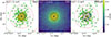 |
Fig. 2. Data (left), simulated PSF (middle), and PSF-subtracted (right) images at the 0.5–2 keV energy band. Dashed red circles indicate the radial bins used for profile extraction, corresponding to the following radii: ∼2″, 2.5″, 3″, 4″, 5.5″, 8.9″, 10.3″, and 11.3″. The QSO position is marked with a black dot, and the shaded black circle represents the 2″ radius used to normalize PSF counts to the data. The annular region between 2″ and 4″ may include approximately 6 background counts. |
The detection of extended X-ray emission around the QSO ID1 was confirmed using both the standard merged event file, aligned with multiple reference sources (Travascio et al. 2025), and the newly merged event file obtained via the refined alignment procedure described in Section 2.2 and Appendix A. Both methods yielded consistent results, though the latter provided a more conservative detection, reducing excess counts within the 2″–4″ annulus by ≲10%. To assess potential PSF estimation errors due to spatial dependencies of the PSF and possible misalignments, we repeated the calculation assuming PSF models estimated from different locations in the field of view. We found that only PSF models generated at positions offset by more than ∼12″ from the QSO location produced a noticeable impact on the radial profiles. This is far larger than any realistic astrometric misalignment in our data (see, e.g. Figure A.1).
Additionally, we tested an alternative approach in which the PSF was directly subtracted from each ObsID’s 0.5–2 keV image before merging, eliminating any potential biases from exposure-weighted PSF stacking. The final PSF-subtracted image remained unchanged, further confirming the robustness of our detection and PSF modelling.
After subtracting the background and the PSF from the QSO image in the 0.5–2 keV band ∼66 ± 8 counts remain, indicating a detection with a significance of ∼8σ. This estimate should be considered a lower limit on the extended emission, as it assumes no diffuse component contributing to the 1492 soft counts observed within the central 2″ (i.e. ∼15 kpc).
3.2. Morphology of the extended X-ray emission
Around the QSO ID1, there is also evidence of warm (T ∼ 5 × 10⁴ K) line-emitting gas in the CGM, as indicated by the Lyα nebula (i.e. MQN01) identified by Borisova et al. (2016), which extends over 200 kpc. If the extended X-ray emission traces hot (T > 106 K) halo gas, this system provides a unique high-redshift case for multi-phase CGM studies, particularly noteworthy given the absence of a detected radio jet, which rules out jet-driven excitation of the Lyα emission. This provides a remarkable example of the potential coexistence of warm and hot gas phases. In this section, we focus on comparing the morphology of the extended Lyα and X-ray emission. Future work will involve a detailed analysis of their physical properties, exploring the implications for gas mass, phase mass fractions, and the underlying processes involved.
Figure 3 shows the smoothed map of the 0.5–2 keV counts, obtained after subtracting the QSO’s PSF contribution as outlined above. The PSF was rescaled to match the sum of the counts within 2″ of the QSO’s centre, which is marked with a black transparent area, while the black filled dot is centred on the QSO with a 1″ radius. The map was smoothed using the aconvolve tool in CIAO-4.15 with a Gaussian kernel of size 2 × 2 native pixels, a normalization factor of 1, and a standard deviation of 1 pixel. The magenta contours trace the Lyα nebula at surface brightness (SB) levels of 2.5, 4, 6, 8, 10 and 12 × 10−18 erg s−1 cm−2 arcsec−2, providing a direct visualization of the nebular extent as related to the X-ray extended emission morphology.
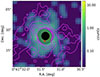 |
Fig. 3. Smoothed soft X-ray 0.5–2.0 keV count map of the extended X-ray emission, obtained after subtracting the QSO’s PSF contribution. The filled black dot marks the QSO centre with a radius of 1″, while the transparent dot represents the inner 2″ region, where counts are used to rescale the PSF to the image. The magenta contours trace the Lyα nebula at surface brightness (SB) levels of 2.5, 4, 6, 8, 10, and 12 × 10−18 ergs−1 cm−2 arcsec−2. The red cross marks the position of the QSO companion detected with ALMA. |
We observe that the majority of the soft X-ray counts are confined within the Lyα SB level of ≈6 × 10⁻¹⁸ erg s−1 cm−2 arcsec−2, and seem to be distributed isotropically, with no preferential directions. The extended X-ray morphology appears to follow the south tail of the Lyα contours, while the east Lyα extension is not connected to any specific X-ray feature. The companion of the QSO ObjB, reported in Pensabene et al. (2024), is located approximately 1″ from the QSO (red cross in Figure 3), well below the extension of the X-ray emission. Moreover, the observations do not indicate the presence of blended X-ray sources.
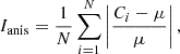
To investigate the spatial correspondence between the extended X-ray emission and the Lyα nebula, within a radial range of 2″–5″, we divided the region into eight sectors and calculated the mean flux in each azimuthal sector, effectively tracing the angular distribution of both components across the selected annulus. We adopt eight sectors to balance spatial resolution and statistical robustness, allowing us to detect potential azimuthal variations in both emissions. The resulting azimuthal profile, shown in Figure 4, shows a comparison of the trends in the normalized fluxes of the X-ray (black) and Lyα (red) emissions. While the X-ray emission does not show statistically significant azimuthal variations, we note that both X-ray and Lyα profiles display a shallow flux minimum near an azimuthal angle of ∼360°. Given the lack of statistical significance, no physical association or spatial alignment can be inferred from this feature. Overall, the X-ray emission remains consistent with isotropy, in agreement with expectations for a virialized or quasi-virialized hot halo. In contrast, the Lyα emission shows a more anisotropic morphology, likely reflecting the clumpy and filamentary distribution of cooler and denser gas phases in the CGM. To quantitatively assess the isotropy of the extended soft X-ray emission, we estimated an anisotropy index (Ianis) in N angular sectors. This index quantifies the average fractional deviation of the photon counts in each sector from a perfectly uniform distribution and is defined as
 (1)
(1)
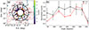 |
Fig. 4. Comparison of the azimuthal flux distribution of the extended Lyα and X-ray emission. (a) PSF-subtracted map of the 0.5–2 keV Chandra X-ray image after subtracting the QSO’s PSF. Red contours show the Lyα SB levels as in Figure 3. Black wedges indicate the sectors used to construct the plot in panel (b). The latter shows the azimuthal distribution of the normalized flux in each 2″–5″ sector, shown as a function of the sector’s central angle. The red curve traces the extended Lyα emission, while the black curve represents the 0.5–2 keV X-ray emission. |
where Ci is the number of counts in the i-th sector, μ is the mean count rate across all sectors, and N is the total number of sectors. To assess deviations from uniformity in the extended emission, we applied both a χ2 test and a Kolmogorov-Smirnov (KS) test to the photon counts distributed in angular sectors. In all cases (including different energy bands and sector choices), we found low isotropy indices (Ianis < 0.4) and high p-values (p > 0.2), with the KS test yielding a maximum D-statistic of 0.093 and p-value = 1. These results consistently indicate there is no statistically significant deviation from isotropy, suggesting that the emission is consistent with being isotropic within current statistical uncertainties.
3.3. Spectral analysis of the extended emission
As a complementary way to investigate and characterize the presence of extended soft X-ray emission, we compare in Figure 5 two spectra: one extracted from the inner 2″ region, where the emission is dominated by the QSO, and one from the 2″–4″ annular region (corresponding to ∼15–30 kpc), where an excess of soft X-ray emission was detected above 2σ in Figure 1. The nuclear spectrum is of high quality, with a count rate of 4.15 × 10⁻³ cts s−1 and a total of 2633 counts, allowing robust spectral fitting. The annular region contains a total of 172 counts in the 0.5–10 keV band and 96 counts in the 0.5-2.0 keV band.
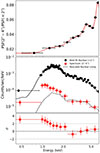 |
Fig. 5. Spectral evidence of excess extended X-ray emission in the soft band, relative to the expected contribution from nuclear (PSF) emission in the 2″–4″ annulus. Top panel: Energy-dependent rescaling factors derived from simulated PSFs, used to estimate the nuclear spillover contribution to the annular spectrum. Middle panel: Spectrum extracted from the central 2″ (black points; binned to at least 50 counts per bin) fitted with an AGN component (solid black line), compared to the spectrum extracted from the 2″-4″ annulus (red points; binned to at least 10 counts per bin), and the predicted nuclear spillover (dashed black line). Bottom panel: Residuals σ in the annulus after subtracting the nuclear spillover component. |
We initially fitted the nuclear spectrum, binning it to a minimum of 50 counts per bin, using the C-statistic (C-stat) and a simple power-law model with Galactic absorption (NH, Gal = 1.15 × 1020 cm−2; Travascio et al. 2025). The analysis was performed with Sherpa (Freeman et al. 2001; Siemiginowska et al. 2024) and cross-checked with XSPEC (Arnaud 1996). The best-fit model without intrinsic absorption yields a C-statistic of 41.19 for 41 degrees of freedom, with a photon index Γ = 2.3 ± 0.1 and a normalization of (2.74 ± 0.36)×10−5. The corresponding χ2 is 38.50 for 43 bins (null hypothesis probability p = 0.582). We also tested the inclusion of intrinsic absorption using the xszphabs model. The fit improves slightly to a C-statistic of 39.75 for 40 degrees of freedom, with a best-fit intrinsic column density of NH, int < 6.25 × 1022 cm−2. The lower bound of NH, int is consistent with zero, and the parameter is fixed at the hard lower limit, indicating that the fit does not require intrinsic absorption. The photon index and normalization remain well determined. The small ΔC-stat of 1.44 for 1 additional degree of freedom confirms that the inclusion of intrinsic absorption does not significantly improve the fit. Therefore, we adopt the simpler power-law model with Galactic absorption only. No evidence of a 6.4 keV iron emission line was found, consistent with at most a negligible contribution from X-ray reflection off cold material in the accretion disk or torus.
Then, we estimated the spillover of nuclear emission into the 2″–4″ annulus. To do it, the best-fit nuclear model was rescaled using energy-dependent correction factors derived from simulated PSFs. These factors, shown in the top panel of Figure 5, represent the ratio of expected PSF counts in the annular region and the central 2″ aperture. The bottom panel of Figure 5 shows the nuclear spectrum (black points), its best-fit model (solid line), the annular spectrum (red points), and the rescaled nuclear spillover component (dashed line). The annular spectrum was binned to a minimum of 10 counts per bin. The comparison shows significant residuals in the annular spectrum after accounting for PSF contribution, particularly below 2 keV, with deviations reaching approximately the 2–4σ level in individual bins. This setup (the AGN model in particular) allows us to perform the spectral analysis of the soft emission.
4. Thermal model of the extended emission
4.1. Spectral and spatial analysis of the extended thermal emission
In this section, we investigate the physical origin of the spectral excess observed in the X-ray emission (see Section 3.3) and its implications for the hot halo in MQN01. The relatively soft and isotropic spatially extended nature of the emission suggests that it may arise from thermal gas heated to X-ray-emitting temperatures by gravitational shocks (or feedback processes) within the QSO halo. Under this assumption, we model the spectral excess using the xsmekal model in Sherpa, which describes the emission from hot, optically thin plasma in collisional ionization equilibrium (CIE). This model incorporates atomic data for thermal bremsstrahlung, recombination, and line emission from highly ionized species (hereafter referred to as thermal CIE emission; see Mewe et al. 1985, 1986; Liedahl et al. 1995). In Section 5.2, we also show that relaxing the assumption of CIE by including the effect of quasar photo-ionization does not affect our results in any way.
We performed a joint spectral and spatial analysis of the extended X-ray emission using Markov chain Monte Carlo (MCMC) methods (e.g. Ruppin et al. 2021), implemented via the Python package emcee (Foreman-Mackey et al. 2013). For the comparison between the models and the data, we used four spectra extracted from concentric regions: the central 2″, and the annuli spanning 2″–3″, 3″–5″, and 5″–8″. The central spectrum was binned to a minimum of 50 counts per bin, while the others were binned to a minimum of 5 counts per bin. These were modelled using a xsmekal model for the extended emission and a power-law component for the nuclear one (i.e. the PSF).
As input parameters of the MCMC fitting, we allowed the plasma temperature (kT), normalization (norm), and metallicity (Z/Z⊙) to vary freely, adopting solar elemental abundances from the Abundanc table in Asplund et al. (2009). We also varied the normalization (normpow) and photon index (Γ) of the power-law component. We did not include intrinsic absorption for this nuclear component, based on the results presented in Section 3.3, where the column density NH is consistent with zero within 1.5σ when fitting the AGN spectrum alone. Nevertheless, even when we include an extended thermal component and allow NH to be a free parameter, the resulting best-fit values remain consistent with the current ones within 1σ, although NH itself remains close to the lowest detectable limit in our data.
The temperature, metallicity, and normalization (norm2, 3) of the xsmekal model are those used to fit the 2″–3″ annular spectrum (red spectrum in Figure 5). While we assume that the metallicity and temperature are constant across all the annuli, the parameter norm2, 3 is proportional to the thermal flux from the 2″–3″ annulus. It is physically related to the average squared gas density integrated along the line of sight (see Equation 4 below). To model the spatial distribution of the thermal gas, we assumed a classical β-model profile (Cavaliere & Fusco-Femiano 1976), commonly used to describe the ICM in low-redshift galaxy clusters (Mohr et al. 1999; Dong et al. 2010; Conte et al. 2011; Paggi et al. 2021). This model is defined as
![Mathematical equation: $$ \begin{aligned} \mathrm{SB}(r) = \mathrm{SB}_{0} \left[ 1 + \left( \frac{r}{r_{\mathrm{core}}} \right)^{2} \right]^{-3\beta + 1/2}, \end{aligned} $$](/articles/aa/full_html/2026/07/aa57020-25/aa57020-25-eq7.gif) (2)
(2)
where β and the core radius rcore are free parameters. The thermal normalizations for each spectrum were computed by scaling the initial norm2, 3 parameter as follows:
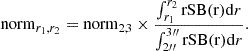 (3)
(3)
Furthermore, we assumed a constant temperature and metallicity at each radius. The normpow parameter was defined in the central region, where the AGN emission is dominant and best constrained, and was then propagated to the outer annuli by rescaling it according to the energy-dependent PSF redistribution (upper panel of Figure 5). This procedure naturally accounts for the radial and spectral redistribution of AGN photons without introducing additional free parameters, as the AGN spectral shape is fixed and only its spatial normalization varies according to the PSF.
We adopted an exponential prior for β (P(β)∝e−β/β*, with β* = 1), motivated by results from local ICM SB profiles as well as in hot CGM around massive galaxies (e.g. Zhang et al. 2024), which typically favour β ≲ 1, with only rare cases reaching values as high as ∼4 (see Mohr et al. 1999; Dong et al. 2010; Conte et al. 2011; Paggi et al. 2021; Xue & Wu 2000; Wise et al. 2004; Mirakhor et al. 2022). A log-uniform (i.e. scale-invariant) prior was assumed for rcore, Z, and for the normalization parameters (norm2, 3 and normpow) to allow for efficient exploration of the parameter space.
To compare the model predictions with the observed counts, we used the Poisson likelihood (aka C-statistics). For each spectrum, we included an explicit background component derived directly from the observed background spectrum, extracted from a large off-source circular region at a projected distance of ∼42″ from the QSO and with a radius of ∼25″. The background was converted to counts per second per kiloelectronvolt using the exposure time and bin widths, and mapped onto the same energy bins as the data. In this way, it is treated directly in detector space, without applying the mirror effective area. We used 100 walkers and 10 000 steps per walker, resulting in a total of 106 samples for the posterior distribution.
Figure 6 shows the marginalized 1D and 2D posterior probability distributions for the model parameters derived from the MCMC. The contours represent the 68.3%, 95.5%, and 99.73% confidence levels. In the histograms, the solid red line indicates the median value of each parameter distribution, while the dashed red lines mark the 16th and 84th percentiles. The median values are also shown in the 2D projections with a red square. As expected, we found a partial degeneracy between the parameters of the xsmekal model (kT and norm2, 3), between the parameters of the nuclear power-law (Γ and normpow) and between those of the beta model (β, rcore). The latter is the most marked, reflecting the absence of deep data at large radii, which would be needed to better constrain the spatial distribution of the gas. The degeneracy between kT and norm2, 3 of the xsmekal model is mostly due to the lack of data at lower energies (at this redshift, we can see with Chandra only the exponential tail of the Bremsstrahlung). Despite these limitations, the marginalized 1D posterior probability distributions are all well behaved and unimodal for all parameters, allowing us to put clear quantitative constraints on the properties of the hot gas. In particular, we found as median temperature and normalization of the thermal component: kT = (1.8 ± 0.4) keV (corresponding to T = (2.1 ± 0.4)×107 K), and  . The nuclear power-law parameters are well constrained, with normpow = (2.1 ± 0.2)× 10−5 and Γ = 2.1 ± 0.1. Note that the best fit slope of the nuclear component is slightly shallower than (albeit within 2σ from) that inferred from the analysis of the nuclear spectrum alone (2.3; Section 3.3), reflecting a small but not entirely negligible contribution of the thermal emission also at small radii (see also Table 2 below). The β-model parameters describing the spatial distribution of the hot gas are
  and
and  . A complete list of the best-fit parameters is provided at the top of Table 1. The only parameter that is loosely constrained by our fit is the metallicity. The posterior probability distribution for this parameter is very broad, reflecting an insufficient S/N for a precise measurement. The posterior probability nonetheless shows a clear preference for relatively low metallicities (Z ≲ 0.1 Z⊙), mainly as a consequence of the non-detection of the Fe Kα complex from He-like and H-like ions at rest-frame 6.7–6.9 keV (observed ≈1.6 keV). We stress, however, that metallicity is included in our MCMC fit only for marginalization purposes, and the formal best-fit value reported in Table 1 should be taken with caution.
 |
Fig. 6. Posterior probability distributions for the simultaneous MCMC modelling of the nuclear and extended emission. Contours represent the 68%, 95%, and 99.7% confidence levels. The vertical solid red lines and the red points mark the best-fit values, which we define as the median value of the distribution of individual parameters, while the dashed red lines mark the 16th and 84th percentiles. Median and percentile values for each parameter are reported above the one-dimensional histograms along the diagonal showing the marginalized distributions for each parameter. |
Best-fit and derived hot halo parameters.
Figure 7 presents the best-fit models (red lines) for the four spectra extracted from the regions defined previously: the central 2″ aperture (top left), and the three concentric annuli 2″–3″, 3″–5″, and 5″–8″, shown in the top right, bottom left, and bottom right panels, respectively. The individual spectral components are plotted separately: the nuclear power-law (blue), background (purple), and thermal (green) components. The residuals in the bottom sub-panels of each spectrum are expressed in terms of σ. The best-fit models reproduce the observed spectra within ∼2σ across all energy bins. However, in the 2″–3″ and 3″–5″ spectra, the models tend to underpredict the emission in the lowest-energy bin (below 0.7 keV). However, emission below 1 keV may be subject to systematic uncertainties related to calibration accuracy, as discussed in Section 4.3.
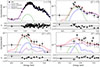 |
Fig. 7. Observed spectra extracted from four regions: the central 2″ aperture (top left), and the 2″–3″, 3″–5″, and 5″–8″ annuli (top right, bottom left, and bottom right, respectively). Overplotted are the best-fit models (red lines) based on the median posterior values from Table 1. The individual spectral components are shown in blue (nuclear power-law), green (thermal emission), and purple (background). Residuals in the lower sub-panels are given in units of σ. |
Table 2 summarizes the soft (0.5–2 keV) and hard (2–10 keV) absorbed fluxes and unabsorbed luminosities of the thermal and nuclear components for each spectrum, assuming best fit (median) parameters, excluding the outermost annulus, where the emission lies below the background level. The results indicate that, within the central 2″ region, the observed thermal soft X-ray flux may account for approximately 12 ± 4% of the total emission in the central 2″. However, this estimate depends sensitively on the β-model parameters.
Observed fluxes and luminosities of the thermal and power-law components.
4.2. Physical properties of the hot halo gas
We used the median posterior values to estimate several physical properties of the system and the hot gas. Assuming that the QSO resides within a virialized dark matter halo, whose virial temperature Tvir is equal to the observed gas temperature, then the implied halo mass would be Mvir ≃ 3 × 10¹³ M⊙ (see Equation (A10) in Dekel & Birnboim 2006). We emphasise that this is a strong and uncertain assumption. Note in particular that if the gas temperature is higher (smaller) than Tvir by a factor f, then the true halo mass is smaller (higher) than the fiducial value by a factor f3/2. Unfortunately, due to the limitations of our data, we are not able to probe deviations of T/Tvir from unity, so we stress that the reported halo mass should be considered as only indicative and taken with caution. The fiducial mass derived in this way is consistent with scaling relations reported in the literature (e.g. Sato et al. 2000; Wang & Abel 2008; Ehlert & Ulmer 2009). The corresponding virial radius (i.e. R200), calculated assuming the same overdensity criterion, is Rvir ≃ 190 kpc, based on Equation (2) from Ehlert & Ulmer (2009).
The electron and hydrogen density distribution in the plasma is related to the best-fit norm2, 3 parameter through the expression4
![Mathematical equation: $$ \begin{aligned} \mathrm{norm}_{r_{\rm in},r_{\rm out}}\ [\mathrm{cm}^{-5}] = \frac{10^{-14} \int _{r_{\rm in}} ^{r_{\rm out}} n_{\mathrm{e}}(r) \, n_{\mathrm{H}}(r) \, \mathrm{d}V}{4 \pi [D_A(1+z)]^2}, \end{aligned} $$](/articles/aa/full_html/2026/07/aa57020-25/aa57020-25-eq50.gif) (4)
(4)
where DA is the angular diameter distance to the source, and the volume integral includes only the region along the line of sight that contributes to the rin − rout annulus in projection. Accounting for the contribution of electrons from helium (0.17 per hydrogen ion, assuming full ionization and a helium mass fraction Y = 0.25), we adopt ne(r)≃1.17 nH(r), making the norm parameter proportional to ∫ne2(r) dV. This expression depends on the electron density profile, which is inferred by deprojecting the observed SB profile under the assumption that the X-ray emissivity scales with ne2(r). For the adopted β-model (Equation 2), the deprojected electron density distribution is
![Mathematical equation: $$ \begin{aligned} n_{\mathrm{e}}(r) = n_{\mathrm{e},0} \left[ 1+ \left(\frac{r}{r_{\mathrm{core}}} \right)^2 \right]^{-\frac{3\beta }{2}}, \end{aligned} $$](/articles/aa/full_html/2026/07/aa57020-25/aa57020-25-eq51.gif) (5)
(5)
where ne, 0 is the central electron density. To relate this 3D density profile to the observed 2D spectral normalization in a given annulus, we perform a proper deprojection of the spherical volume intersected by the line of sight through the annulus. Specifically, we compute the volume integral in Equation (4) using cylindrical co-ordinates (R,ϕ,z), where the volume element is dV = RdR dϕ dz and  . The azimuthal integration yields a factor 2π, using the analytical form of the line-of-sight projection for spherically symmetric functions, commonly known from the Abel transform framework, we obtained
![Mathematical equation: $$ \begin{aligned} \int n_{\mathrm{e}}^2(r) \mathrm{d}V = \frac{4 \pi r_{\mathrm{core}}^3 n_{\mathrm{e},0}^2}{\beta _0 \,\ \tilde{\chi }(3 \beta )^{-1}} \Biggl [ \Biggl ( 1 + \frac{r_{in}^2}{r_{\mathrm{core}}^2} \Biggr )^{-\frac{\beta _0}{2}} - \Biggl ( 1 + \frac{r_{\rm out}^2}{r_{\mathrm{core}}^2} \Biggr )^{-\frac{\beta _0}{2}} \Biggr ], \end{aligned} $$](/articles/aa/full_html/2026/07/aa57020-25/aa57020-25-eq53.gif) (6)
(6)
where β0 = 6β − 3, while the function  is defined as:
 (7)
(7)
A proof of the last equality in Equation (7) is provided in Appendix C. Note that  is related to the function χ defined in Pezzulli et al. (2017) by the relation
  .
.
This formulation (6) accurately captures the projection of the spherical density distribution into the annular region observed in the sky. By inserting this expression into Equation (4), we derived a direct relationship between the central density and the observed spectral normalization in the ne, 0 corresponding rin-rout annulus:
![Mathematical equation: $$ \begin{aligned} n_{\mathrm{e},0} = \sqrt{ \frac{1.17 \times 10^{14}\, [D_A(1+z)]^2 norm_{r_{\rm in},r_{\rm out}} \, \beta _0}{r_{\mathrm{core}}^3 \, \tilde{\chi }(3 \beta ) \, [ ( 1 + r_{\rm in}^2/r_{\mathrm{core}}^2)^{-\frac{\beta _0}{2}} - ( 1 + r_{\rm out}^2/r_{\mathrm{core}}^2)^{-\frac{\beta _0}{2}} ]} }, \end{aligned} $$](/articles/aa/full_html/2026/07/aa57020-25/aa57020-25-eq58.gif) (8)
(8)
where DA and rcore are expressed in cm, normrin, rout in cm−5 and ne, 0 in cm−3. Applying this method, we estimated a central electron density of  .
.
We then computed the total mass of hot gas within the virial radius using
![Mathematical equation: $$ \begin{aligned} M_{\mathrm{hot\,gas}} = \frac{4 \pi \, n_{\mathrm{H},0} \, m_p }{X} \int _0 ^{R_{\mathrm{vir}}} r^2 \, \Biggl [ 1 + \Biggl ( \frac{r}{r_{\mathrm{core}}} \Biggr )^2 \Biggr ] ^{-3 \beta /2} \mathrm{d}r, \end{aligned} $$](/articles/aa/full_html/2026/07/aa57020-25/aa57020-25-eq60.gif) (9)
(9)
where nH, 0 = ne, 0/1.17, mp = 8.4 × 10−58 M⊙, and X = 0.75 the hydrogen mass fraction. This yields a hot gas mass of  corresponding to a hot baryon fraction of
  . Assuming a cosmic baryon fraction fb = Ωb/Ωm = 0.15 (e.g. Mohr et al. 1999; Gonzalez et al. 2007; Ettori et al. 2009; Hinshaw et al. 2013; Ge et al. 2018) this implies that the hot gas accounts for
  of the baryons primordially associated with the halo. This fraction highlights that a substantial part of the halo’s theoretical baryon budget is found in the hot CGM phase. Here, by baryon budget, we refer to the total baryonic mass expected from the cosmic baryon fraction to be associated with the halo’s dark matter, independent of whether these baryons are currently located inside or outside the virial radius. This fraction is consistent with observations of low-mass groups and intermediate-mass clusters in the local Universe, where the hot gas typically accounts for about 30–85% of the halo’s baryonic content (e.g. Eckert et al. 2013; Morandi et al. 2015; Pratt et al. 2023). The fact that a similarly large mass of hot CGM is found already at z ∼ 3, co-existent with a luminous Giant Lyα nebula, is in line with the predictions of Pezzulli & Cantalupo (2019), who explored the role of hot virialized gas in boosting the Lyα emissivity in MUSE QSO nebulae (including MQN01) through the compression of colder (Lyα-emitting) gas. This is further discussed in Section 5.5.
The total hot gas mass and baryon fraction rely on the assumption that the observed X-ray emission within 38 kpc is only the brightest inner portion of a more extended halo, which is well described by our β-model, up to the virial radius. Note, however, that the total soft X-ray luminosity extrapolated to the virial radius, L0.5 − 2 keV(< Rvir)≃2.27 × 1045 erg s−1, is only 3% higher than the luminosity measured within 5″ of the central QSO. This shows that, despite the large extrapolation in radius, the correction in luminosity is minimal. In our best-fit model, most of the gas mass (about 55%, as reported in Table 1) is already enclosed within 38 kpc (i.e. 5″).
4.3. Systematic uncertainties on the X-ray luminosities
An important aspect to consider is the presence of systematic uncertainties affecting the measurement of the soft X-ray luminosities (Table 2). The detection of extended thermal emission in the 0.5–2 keV rest-frame band may be susceptible to the shape of the spectral continuum at low energies, where the effective area of Chandra drops significantly. Since the thermal component is mainly constrained by photons below ∼2 keV, any small number of counts or calibration inaccuracy in this range, although unlikely to fully mimic the observed signal, can steepen the spectral fit and bias the extrapolated luminosity estimate. Here, we are explicitly considering only the conservative case in which calibration uncertainties would reduce the inferred soft X-ray luminosity. However, it is worth noting that our main MCMC model already underpredicts the low-energy counts (see residual for the lowest energy bin in Figure 7), suggesting that any such systematic would only bring out the model in better agreement with the data. More generally, the mere detection of soft X-ray emission at such a high redshift, where the observed energy range samples only the high-energy tail of the thermal bremsstrahlung spectrum, already implies that the emission must be intrinsically powerful.
Nonetheless, to mitigate any unmodelled systematics related to the lowest energy bin, we repeated the MCMC analysis using only the spectral data above 1 keV (observed frame), where the Chandra effective area is more stable and remains above 60 cm2. In this alternative fit, we applied a Gaussian prior on the temperature, centred at kT = 2.5 keV (i.e. 64% higher than the previous best-fit value) with a standard deviation of 0.5 keV. Imposing a prior with a higher temperature than our fiducial model is a conservative choice, as a higher temperature implies a shallower spectral slope, thereby reducing the extrapolated soft-band luminosity. Under these assumptions, the posterior distribution for kT peaks around ≈1.9 keV, with the corresponding total luminosity, within 30 kpc, reaching a minimum of ≈1045 erg s−1 within 1σ. This test shows that, even when conservatively accounting for potential calibration systematics and introducing an explicit bias in favour of high temperatures, relatively low temperatures are still preferred and the inferred intrinsic soft-band luminosity remains significantly high.
5. Discussion
5.1. Impact of the QSO radiation on the thermal emission
Throughout our X-ray spectral analysis, we have implicitly assumed that the hot gas is in CIE. At the temperature (kT ∼ 1.8 keV) and metallicity (Z/Z⊙ ∼ 0.01) inferred for the extended emission, hydrogen and helium are fully ionized and metal-line emission is extremely weak. Under these conditions, photoionization from the central QSO is not expected to affect the ionization balance or the thermal continuum in any significant way. To verify this expectation, we performed test calculations with the code Cloudy, modelling a representative gas shell at r = 15 − 23 kpc exposed to the observed QSO spectral energy distribution (SED; “AGN T=1.8e5 K a(ox) = –0.6 a(uv) = –2 a(x) = -1.9”) constrained to match UV (νLν(1700 Å) = 6.5 × 10⁶ erg s−1; Borisova et al. 2016) and X-ray (νLν(2 keV) = 3.3 × 1045 erg s−1; Travascio et al. 2025) photometric measurements, adopting a X-ray power law photon-index of Γ ≈ 2.1. The resulting thermal spectrum was compared with that predicted by a standard CIE model (xsmekal) with the same density, temperature, and metallicity. The differences in the 0.5–2 keV band were found to be negligible (< a few percent), confirming that QSO photoionization has no measurable impact on the X-ray emission in this regime (see details in Appendix D).
We also explored time-dependent Cloudy simulations, by allowing a non-equilibrium cooling (set dynamics relax 3) and by tracking the thermal evolution over 300 iterations, to evaluate whether the QSO radiation field could significantly modify the cooling time of the gas. The inclusion of photoionization increased the cooling time by only ≈10%, a marginal effect that does not alter any of our conclusions. We therefore conclude that the CIE assumption adopted throughout this work is fully justified.
5.2. Alternative scenarios for the extended soft X-ray emission
We developed analogous models to those of the previous section in which the hot thermal gas is replaced by cold clouds photoionized by the QSO, exploring a grid of gas densities and metallicities. We have verified that the emission from these photoionized clouds fails to account for the observed extended X-ray excess, even under the extreme assumption that the cold phase occupies all the volume with filling factor fV = 1. A more detailed analysis of these models, including constraints derived from the Lyα nebula, will be presented in a future paper, as this lies beyond the scope of the present work.
We tested a non-thermal IC scenario, fitting the X-ray excess with a power law, which results in unphysically steep photon indices of Γ ∼ 6 (see Worrall et al. 2016), and found no evidence of powerful radio jets associated with this QSO (e.g. Sydney University Molonglo Sky Survey at 843 MHz; Mauch et al. 2003, and 0.8 mJy/beam at 1.367 GHz and 0.78 mJy/beam at 887.5 MHz in the Rapid ASKAP Continuum Survey).
We also explored a scenario in which the extended X-ray emission originates from thermal Compton up-scattering of AGN seed photons by a hot electron population produced by an extended AGN wind, modeled using compTT. To reproduce the spectral shape of the extended X-ray emission, we assumed, as a conservative scenario, seed photons representative of the standard soft X-ray excess commonly observed in local AGN, typically peaking around ∼0.1 keV rest-frame (Crummy et al. 2006; Done et al. 2012). We adopted an optical depth of τ = 0.01, which is the upper limit derivable from our constraint on the electron column density in the X-ray quasar spectrum, corresponding to an electron density of ne = τ/(1 σT) ∼ 0.3 cm−3, where l ∼ 15 kpc and σT = 6.65 × 10⁻²⁵ cm2 is the Thomson cross-section. From spectral fitting, we obtained  and
and  . This model reproduces the observed extended emission with a required Lseed ≈ 2 × 1046 erg s−1, about a factor of two lower than the UV luminosity at 1700
Å. However, we can rule out this scenario for two main reasons. First, a plasma with such high energy and density would inevitably produce a Bremsstrahlung emission at a level approximately two times higher than observed, in addition to the measured signal. Second, assuming that this energetic electron population is thermal and homogeneously distributed as a sphere of radius 30 kpc, we would expect a 15σ SZ detection, which is not observed, as further discussed in the next section.
. This model reproduces the observed extended emission with a required Lseed ≈ 2 × 1046 erg s−1, about a factor of two lower than the UV luminosity at 1700
Å. However, we can rule out this scenario for two main reasons. First, a plasma with such high energy and density would inevitably produce a Bremsstrahlung emission at a level approximately two times higher than observed, in addition to the measured signal. Second, assuming that this energetic electron population is thermal and homogeneously distributed as a sphere of radius 30 kpc, we would expect a 15σ SZ detection, which is not observed, as further discussed in the next section.
5.3. Constraints from SZ non-detection
The detection of extended X-ray emission suggests the presence of hot gas within a ∼ 3 × 10¹³ M⊙ halo, potentially producing a thermal SZ effect (Sunyaev & Zeldovich 1972). However, an analysis of ALMA Band 3 data (Pensabene et al. 2024) reveals no clear evidence of an SZ signature in the current observations. To estimate the expected SZ significance (σSZ), we generate the SZ signature for each set of β-model parameters, kT, and ne from the previous analyses, and inject the resulting models into jackknifed realizations of the available ALMA data (see Di Mascolo et al. 2023; van Marrewijk et al. 2025, for details on the jackknifing procedure). Our analysis indicates that the non-detection within the sensitivity limits of the current ALMA data is fully consistent with the hot gas properties as derived by the X-ray analysis. The posterior parameters from the MCMC analysis predict a marginal SZ signal with a significance of only ≃(2.6 ± 0.4) σSZ. Additionally, continuum emission from companion quasars and deviations from thermal pressure support could further suppress the SZ signal, potentially explaining the current non-detection. New ALMA Cycle 12 observations (Project ID: 2025.1.00107.S, priority grade B) have been awarded to our team. These data, once executed, will provide the sensitivity and angular resolution needed to further probe the thermal and non-thermal components of the ICM and to test more robustly the presence of an SZ signal in this system.
5.4. Comparison with Spiderweb and simulated hot halos
Studying the nascent hot phase of the CGM (or proto-ICM) in z > 2 halos is difficult because it requires long integration times with current X-ray telescopes. Previous to this work, the only reported direct imaging detection of extended thermal ICM emission at z > 2 was around the Spiderweb galaxy in ≈700 ks, L24, who reported residual extended emission after the subtraction of the X-ray IC emission due to radio jets. For both Spiderweb and MQN01, the extended thermal emission appears to originate from the halo of a proto-BCG at the center of a forming (or proto-)cluster. Comparing luminosity, density, and morphology of these systems at z = 2.16 and z = 3.25 could provide some insights into the possible evolution of the hot CGM, alternatively referred to as the proto-ICM, with redshift and with their halo properties. Following the approach of L24, we computed the average SB of the extended X-ray emission in concentric annuli using
 (10)
(10)
where Aann is the area of the annulus, texp is the total exposure time, and the ratio ExpMapmax/ExpMapann ≈ 1 accounts for small variations in the Chandra sensitivity within the relevant portion of the field of view. The energy conversion factor (ECF) depends on the temperature and metallicity parameters of the xsmekal model used to fit the spectra. The extended X-ray SB profile was obtained by subtracting the PSF-derived profile from the data. We estimated the SB profile in the 0.5–2 keV band (hereafter SBX(r)) for the extended X-ray emission around QSO ID1 in the MQN01 protocluster. This used an ECF of ∼4.6 × 10⁻¹¹ erg cm−2cnts−1, based on the best-fit temperature (kT ∼ 1.8 keV), and 0.014 Z⊙ from our MCMC fit (see Section 4). As indicated by the MCMC results, the PSF model was normalized to match the observed counts within the central 2″ (i.e. ∼15 kpc), under the assumption that ∼12% of the total emission originates from thermal processes (i.e. fth = 0.12; see Table 2).
Figure 8 shows the redshift-dimming corrected SBX(r) of the extended X-ray emission in MQN01 (red) and Spiderweb (blue). The red dots, indicating the SBX(r) of the MQN01 halo, consist of three data points measured between 15 and 30 kpc (i.e. 2″-4″; where the extended residual X-ray emission is detected following the subtraction of the nuclear emission), one point within 15 kpc (< 2″; shaded grey region), which is extrapolated from the best-fitting β model (see Section 4), and upper limits at all radii above 30 kpc. The SBX profile of the X-ray extended halo in Spiderweb is taken from L24. To correct for different rest-frame bands due to redshift, we applied a 0.536 factor to the Spiderweb SBX(r) halo. This factor was derived assuming the best-fit kT = 2 keV xsmekal model reported in Tozzi et al. (2022). The black lines show the SBX(r) profiles of simulated hot halos, where the solid, dashed, and dotted lines represent the median, 16th-84th percentile, and full range (minimum to maximum) of the SBX profiles, respectively. These profiles were computed from a sample of 12 halos at z = 3 extracted from the DIANOGA cosmological hydrodynamical simulations of galaxy clusters (Esposito et al. 2025). This version of the DIANOGA simulations includes 14 target clusters at z = 0, in the mass range (0.2−3) × 1015 M⊙, simulated with OpenGADGET-3 (e.g. Groth et al. 2023; Damiano et al. 2024). The 12 halos were selected in the mass range (2−6) × 1013 M⊙ to have a median mass matching the virial mass of the MQN01 halo (Mvir ∼ 3 × 10¹³ M⊙). The X-ray maps of the simulated halos were obtained with the post-processing tool SMAC (Dolag et al. 2005) in cubic regions of 500 kpc per side around the center of each halo, with 1 kpc resolution.
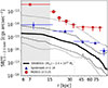 |
Fig. 8. Redshift-dimming corrected X-ray SB profiles in the observed 0.5–2 keV band (SBX) for the extended thermal emission around QSO ID1 (red circles), obtained using an energy conversion factor (ECF) of ≃4.6 × 10⁻¹¹ erg cm−2 cnts−1 based on the best-fit values of kT = 1.8 keV and Z/Z⊙ = 0.014, and for the Spiderweb Galaxy (blue triangles) L24. A correction factor of 0.536 was applied to the Spiderweb hot halo’s SBX profile from L24 to account for differences in the redshift-dependent intrinsic energy band. The black lines show the median (solid), 16th–84th percentile (dashed) and minimum-maximum (dotted) SBX profiles of hot halos at z = 3 from the DIANOGA simulations, selected to have an average mass consistent with the estimated virial mass of the MQN01 halo (i.e. ∼3 × 10¹³ M⊙). |
While the SBX profiles of MQN01 and Spiderweb differ significantly in normalization, by a factor of 3-10 within 30 kpc of the QSOs, MQN01’s profile is also noticeably steeper, consistent with a highly compact core. The SBX profile in MQN01 is consistent, for r > 20 kpc, with the upper envelope of the SBX profiles from DIANOGA simulations. Similarly, the SBX profile of the Spiderweb halo closely follows the 84th percentile of the distribution from the DIANOGA hot halos. Within the limited statistics, simulations predict fainter and shallower SBX profiles than the two observed. Part of the reason for this discrepancy may lie in the different sub-grid prescriptions adopted in the simulations. In particular, the DIANOGA runs use a relatively low density threshold for star formation (0.13 cm−3), which inhibits the formation of high-density gas regions, especially near halo centres. To test the impact of this, we compared the hot gas density profiles from DIANOGA with those of the most massive halos at z = 3 in the DaLya simulations (priv. comm., Lazeyras et al., in prep.), which adopt a star formation threshold 100 times higher. For a consistent comparison, we applied the same temperature cut (kT > 0.1 keV) as in the DIANOGA analysis to isolate the X-ray-emitting hot phase in both simulations. We found that the density of kT ∼ 0.1 keV gas in DaLya is 5–10 times higher than in DIANOGA.
Figure 9 compares electron density, ne(r) (top panel), and pressure, Pe(r) (bottom panel), profiles, of hot halos in MQN01 (red line and black dots), Spiderweb (blue), and DIANOGA simulations (green). The red curves show the best-fit profiles for the MQN01 halo, with the shaded area indicating the 68% confidence interval from Monte Carlo realizations on ne, 0, β, rcore, and kT. The ne(r) and Pe(r) profiles of the Spiderweb hot halo, with the relative uncertainties, are from L24, while DIANOGA profiles are directly extracted from simulations.
 |
Fig. 9. Electron density (ne(r)) and pressure (Pe(r)) profiles of the hot halos in MQN01 (red), Spiderweb (blue), and DIANOGA simulations (green). The red curve shows the best-fit model for MQN01, with the shaded region indicating the 68% confidence interval. The profiles of the Spiderweb halo is from L24, while the green band represents the range of profiles extracted from DIANOGA cosmological simulations of massive halos (∼2–6 × 10¹³ M⊙) at similar redshift as MQN01 (i.e. z = 3). The dashed vertical red lines indicate the radial range between 2″ and 5″, where we observe a significant detection. |
Between 15 and 30 kpc, the electron density of the MQN01 hot halo exceeds that of the Spiderweb halo by a factor of 4.3 ± 1.0 on average. At 15 kpc the ratio is 4.9 ± 3.1, decreasing to 3.5 ± 4.5 at 30 kpc. In the same radial range, the pressure of the MQN01 hot halo reaches values 5–10 times higher than those measured or predicted in the other cases. Specifically, the Pe(r) profile of the Spiderweb halo, which benefits from an independent pressure estimate based on SZ observations (Di Mascolo et al. 2023), is consistent with the predictions of the DIANOGA simulations, lying at the upper end (i.e. 84th percentile) of the distribution.
However, it is important to emphasize that, while other factors such as feedback prescriptions, star formation threshold, and numerical resolution may contribute to these discrepancies, current X-ray observations at these redshifts are limited both in sensitivity and in the availability of similarly deep Chandra data for hyperluminous QSOs. As a result, it is not yet possible to assess whether the systems considered here are representative of the proto-ICM population or instead trace its extreme tail. Consequently, interpreting the higher normalization of the observed profiles relative to DIANOGA simulations as a genuine physical discrepancy should be treated with caution, as it may not reflect the properties of the overall proto-ICM population.
5.5. Pressure confinement of cold CGM clouds
The hot gas pressure at 15 kpc and 30 kpc, which are the minimum and maximum radii at which we directly observe the extended X-ray emission based on our analysis, is  and 0.30−0.12+0.53 keV cm−3, respectively. These are about one to two orders of magnitude higher than typical values observed for the ICM in local galaxy clusters (Ettori et al. 2009), and about three-to nine-fold higher than those obtained for the hot halo in Spiderweb (i.e. < 0.1 keV cm−3, L24) from independent measurements using ALMA SZ observation (Di Mascolo et al. 2023). Such a high thermal pressure is sufficient to confine the cold, Lyα -emitting phase of the CGM. Assuming pressure equilibrium and a cold gas temperature of Tcold = 5 × 10⁴ K, the implied temperature ratio Thot/Tcold ∼ 400 leads to a density contrast of the same factor. Therefore, for a hot gas density of nhot = 0.1 cm−3 at ∼50 kpc (see Figure 9), the warm gas can reach densities up to ncold ∼ 40 cm−3, supporting a scenario in which the Lyα nebula in MQN01 arises from a distribution of dense clumps pressure-confined by the surrounding hot halo (Pezzulli & Cantalupo 2019; Cantalupo et al. 2019), at least in the CGM inner regions. We stress, however, that our results (in particular the exceptionally high densities) may not be representative of the average Lyα nebulae detected so far around luminous z ∼ 3 quasars, as the latter do not generally reside in overdensities as large as that of MQN01 and their halo masses are expected to be, on average, smaller than what is derived for MQN01 (Pezzulli & Cantalupo 2019; de Beer et al. 2023).
5.6. Comparison with local galaxy groups and clusters
Here, we briefly compare our results with the properties of the ICM of local groups or clusters. From our best-fit model in Section 4.1, we obtained a ratio rcore/Rvir≈0.2, which falls within the typical range of 10−2 to 0.6 observed for the ICM in local galaxy clusters and groups (e.g. Vikhlinin et al. 2005). The same model yields a value of β higher than the typical one observed in local systems (∼0.7), although consistent within 1.6σ.
Figure 10 shows the relation between L0.5 − 2 keV5 and kT for a variety of massive structures, including low- and high-redshift systems ranging from galaxy groups to rich clusters. Notably, the red square represents the average temperature and X-ray luminosity of the extended X-ray emission in the Spiderweb protocluster ( , L0.5 − 2 keV = (2.0 ± 0.5)×1044 erg s−1). The Spiderweb point falls within the scatter of the group and cluster population, although the temperature is likely overestimated compared to the SZ-based value (kTSZ = (0.7 ± 0.3) keV Di Mascolo et al. 2023). Adopting the lower SZ-based temperature would shift the Spiderweb point even further above the typical relation. The extended X-ray emission analysed here at z = 3.25 (red circle) shows a notably higher 0.5–2 keV luminosity than other structures with comparable temperatures, even after accounting for uncertainties on the fth value, placing MQN01 well outside the typical distribution of hot gas in groups and clusters.
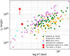 |
Fig. 10. Soft X-ray (0.5–2 keV) luminosity versus temperature kT of the ICM in massive structures across redshift. Symbols show galaxy clusters from Bulbul et al. (2019) (green squares), O’Hara et al. (2007) (orange triangles), Mittal et al. (2011) (magenta crosses), and high-redshift clusters from the literature (cyan triangles; Stanford et al. 2001; Fabian et al. 2001; Mathur & Williams 2003; Andreon & Huertas-Company 2011; Tozzi et al. 2015; Mastromarino et al. 2024). The red square marks the Spiderweb protocluster hot X-ray halo (L24), while the red circle shows the value for the X-ray halo in this work (MQN01) within a radius of 8″, respectively. The background density distributions represent the conservative MCMC posterior accounting for systematics (Section 4.3). |
One possible explanation for the observed high luminosity could be related to redshift evolution. In particular, the self-similar evolution model (see Maughan et al. 2012, where LX ∝ E(z) as first approximation) predicts luminosities of ∼ 6.3 × 1043 erg s−1 for Spiderweb and ∼ 4.1 × 1044 erg s−1 for MQN01. This provides a baseline to compare with local groups and clusters, under the assumption that the self-similar model applies. However, we note that this evolution is formally derived for bolometric luminosities, whereas our comparison is carried out in the soft band. Since the fraction of the bolometric luminosity falling in the soft band depends on the plasma temperature, applying the self-similar scaling directly to soft-band luminosities can overestimate the true redshift evolution, particularly for low-temperature systems. Even accounting for this, the MQN01 point remains significantly above the local LX-T population, while the Spiderweb point appears broadly consistent with it.
Within the framework of thermal bremsstrahlung and line emission, this is not surprising, since we are probably observing a distinct and earlier phase of the ICM, which is characterized by different physical conditions. As discussed in Section 5.4, given the sensitivity limits of current X-ray observations and the lack of similarly deep data for z > 3 hyperluminous QSOs, it remains unclear whether this pronounced deviation reflects genuine evolutionary effects or simply the properties of a small sample and potentially unrepresentative system.
5.7. Thermal instability and hot halo condensation
In this work, we have presented the first detection of extended hot (T ≳ 107K) gas in a massive halo at z > 3. Cosmological theory (e.g. Dekel & Birnboim 2006) predicts that such structures should form as a consequence of the virialization of gas infalling onto dark matter haloes from the IGM and being shock-heated as a result of the collision of multiple infalling gas streams. The early cosmic time of our observation, along with with the peculiarly compact structure (see Section 5.4), leads us to speculate that we may be witnessing the initial stages of the formation and virialization of a hot halo, possibly leading, through further gas accretion and the expansion of the shock front to larger radii, to the more extended hot gas structures typically observed in the nearby Universe.
At the same time, the extreme luminosity of MQN01 (see Figure 10), indicative of large radiative losses, also raises the question of whether some of the recently virialized gas may already be undergoing substantial cooling, possibly contributing to the fueling of star formation and AGN activity in the central galaxy. A similar interpretation has been discussed by L24 in the context of the hot halo of Spiderweb at z ≃ 2.16, based on the inferred low temperatures (T ∼ 0.3–0.9 keV) and short cooling times (< 100 Myr)6. In addition, L24 report a nominal isobaric mass deposition rate of Ṁcool ≈ 0.25–1 × 10³ M⊙ yr−1, which exceeds typical cooling rates inferred for low-redshift ICMs (McDonald et al. 2018), although it does not account for heating or feedback processes.
Similarly, applying the same steady-state, isobaric cooling-flow formalism to MQN01 (Equation (2) Fabian 1994), and using  (as in Jones & Forman 1984), would result in a mass deposition rate of
  in this central region. This estimate assumes that the entire X-ray-emitting gas cools efficiently and steadily, and should be interpreted as an upper limit. We emphasise that these estimates ignore any source of heating or mechanical energy injection (e.g. AGN feedback, turbulence), which are thought to largely compensate for the cooling, so that the nominal mass deposition rates can be overestimated by factors 10–100 (e.g. Fabian 1994; Gaspari et al. 2013). Moreover, a sustained mass accretion rate of ≃ 103 M⊙ yr−1 could at most occur episodically. Indeed, if maintained for 1 Gyr, it would lead to an accumulation of 1012 M⊙ of cold gas, exceeding that observed in any known galaxy.
To assess whether a less extreme scenario of localized thermal condensation is likely in our hot halo in MQN01, we compared the radiative cooling time, tcool, to the dynamical free-fall time, tff, at r = 15 and 30 kpc. The ratio tcool/tff is a widely used diagnostic for precipitation and/or condensation in hot halos (e.g. Voit et al. 2015; Choudhury & Sharma 2016; Voit et al. 2017; Stern et al. 2021; Donahue & Voit 2022). Using the ‘classical’ formula (as shown by Donahue & Voit 2022) and a representative cooling function Λ(T, Z)≃10−23 erg cm3s−1, we found tcool(15 kpc) = 55−14+24 Myr and tcool(30 kpc) = 181−83+268 Myr. Estimating tff from the local gravitational field (e.g. McCourt et al. 2012; Wibking et al. 2025), which we computed assuming a NFW potential with a concencentration c ≃ 3.5 ± 0.5 (as suggested by Correa et al. 2015, for a 1013 M⊙ halo at z ≈ 3) we obtained tff(15 kpc) = 36−4+5 Myr and tff(30 kpc) = 58−5+8 Myr. These yield ratios tcool/tff(15 kpc) = 1.9−0.9+1.9 and tcool/tff(30 kpc) = 3.1−1.4+4.6. All fall within the commonly cited precipitation threshold, 1 < tcool/tff < 10, under which local thermal instabilities can seed multiphase condensation in roughly hydrostatic, feedback-regulated atmospheres (Donahue & Voit 2022).
We note that, despite its common usage in the literature, the free-fall time tff is not strictly the most relevant timescale for local thermal instabilities. A more direct indicator of potential condensation is the Brunt-Väisälä time tBV, which is the timescale for the reaction of buoyancy against thermal instability. While tff and tBV are often comparable in compact halo cores, tBV remains a more precise diagnostic because it is defined locally through perturbation analysis (e.g. Nipoti & Posti 2014; Wibking et al. 2025). To compute tBV, we used Equation (D3) in Appendix E, again assuming the gravitational field g associated with the NFW potential. We found tcool/tBV(15 kpc) = 1.3−0.5+1.0, and tcool/tBV(30 kpc) = 4.5−2.4+8.7, which are still in the range 1 < tcool/tBV < 10. This does not imply a global cooling catastrophe, but it is consistent with intermittent condensation in portions of the hot halo that can feed cold inflows and/or SMBH fueling. Note, however, that classic analyses demonstrate that buoyancy in atmospheres with positive entropy gradients can suppress linear thermal instability (Binney et al. 2009). Recent simulations (see Wibking et al. 2025) further suggest that whether condensation occurs depends on turbulence, mixing, and the geometry of heating. Some systems with tcool/tff ≲ 10 can remain stable if turbulent support is weak or heating is centrally concentrated (see discussions in Donahue & Voit 2022). Consequently, our results should be interpreted as strong plausibility for localized condensation, contingent on the local balance of turbulence, mixing, and feedback.
To further probe the dynamical state of the hot gas halo, we examined the balance between the pressure gradient force and the gravitational acceleration derived from the NFW dark matter profile. Using the MCMC posterior parameters of kT, rcore, and Mvir with their associated uncertainties, we computed the ratio of the hydrostatic acceleration from the pressure gradient, 1/ρ(dP/dr), to the gravitational acceleration, g(r), at radii of 15 and 30 kpc. Our Monte Carlo analysis, sampling the uncertainties, yields ratios of ≃0.7−0.5+1.4 at 15 kpc and ≃1.3−0.8+1.7 at 30 kpc, consistent with hydrostatic equilibrium, although significant deviations are allowed within the credible intervals. These results suggest that, while the hot gas is roughly in hydrostatic balance, there may be local departures indicative of dynamical processes such as inflows, outflows, or turbulence. Such deviations can enhance thermal instability and promote condensation, consistent with the 1 < tcool/tff < 10 found above. Therefore, the combined diagnostics support a scenario in which the hot halo is marginally stable, possibly allowing localized cold gas condensation and potentially fueling galaxy growth and AGN activity.
We emphasize that all physical quantities reported here should be regarded as rough estimates with large uncertainties, given the limited number of detected thermal photons (66). A more robust characterization of the thermal state of the proto-ICM in MQN01 will require deeper observations.
6. Summary and conclusions
In this paper, we report a significant (at least 8σ between 15–30 kpc) detection of 0.5–2 keV (∼2–8 keV rest-frame) X-ray emission, extended out to ∼ 30 kpc, around the brightest QSO (ID1) within the MQN01 protocluster at z = 3.25 (Section 3). This QSO is also surrounded by a giant (> 200 kpc) Lyα nebula (#1 in Borisova et al. 2016). The extended X-ray emission exhibits a morphology consistent with isotropy (Section 3.2).
The steepness of the spectrum and the isotropic morphology of the extended X-ray emission suggest a thermal origin, with the emission powered by bremsstrahlung and collisional excitation mechanisms. Alternative emission mechanisms, such as photoionization of the hot gas clouds by the AGN, IC scattering, or Compton up-scattering, fail to fully or even partially reproduce the observed extended X-ray excess, as discussed in Section 5.2. Therefore, this likely represents the first evidence of thermal emission from proto-ICM (or hot CGM) at z > 3.
If the QSO resides within a virialized halo, whose virial temperature is equal to the observed gas temperature, and further assuming that the detected emission traces the brighter inner region of a gas distribution extending to the virial radius, we can infer the halo mass and hot gas content. However, these inferences rely on extrapolating the emission beyond the observed region and should therefore be treated with caution. We performed a joint spatial and spectral MCMC analysis. The median posterior values imply the following (Section 4):
-
A temperature of ≈1.8 keV corresponding to a virial halo mass of Mvir ≃ (3 ± 1)×1013 M⊙, under the assumptions of a virialized halo and that the gas temperature equals the virial temperature.
-
Hot gas within 30 kpc exhibits electron densities ranging from 0.9 to 0.2 cm−3 and a 0.5–2 keV X-ray luminosity of L0.5 − 2keV = 2.25−1.38+0.77 × 1045 erg s−1.
-
The spatial fit yields β-model parameters of core radius
 and
and  . The latter is higher than (but consistent within 1.6σ with) the typical β = 0.7 observed in local galaxy groups and clusters, indicating a steeper gas density profile.
 -
The analysis implies that the hot gas in the halo of MQN01 contains a substantial fraction,
 , of the baryons that are theoretically associated with the halo (i.e. the baryonic mass that one would expect assuming a cosmic baryon fraction Ωb/Ωm ≃ 0.15).
Despite the large uncertainty, the last result, united to the fact that some baryonic mass must also be stored in the colder (Lyα-emitting) phase of the CGM, suggests that the halo of MQN01 contains a substantial fraction of its theoretical baryon budget within the virial radius. We plan to better quantify the total baryon budget of MQN01 in a future combined analysis of both the X-ray and Lyα emission.
Based on our results, the currently available ALMA data are not expected to allow for a clear detection of any thermal SZ signal, as the expected significance is only (2.6 ± 0.4) σSZ, even assuming perfect subtraction of contaminating sources (Section 5.3). However, upcoming tailored ALMA observations will be able to confirm (or challenge) our findings and add further constraints on the spatial distribution and thermal state of the hot gas in MQN01.
MQN01’s hot halo is notably brighter and denser than that in the Spiderweb protocluster at z = 2.16 L24, with X-ray surface brightness and electron density profiles exceeding those of Spiderweb by factors of 3–10 and 3–5 times within 30 kpc. These differences may reflect cosmic evolution in density and increased gas clumpiness.
Compared to cosmological simulations (DIANOGA), MQN01’s halo represents the luminous extreme of predicted hot halos, with higher densities possibly linked to a too low density threshold of star formation assumed in the simulations, which prevents dense gas from remaining in the X-ray emitting phase (Section 5.4). On the other hand, the total X-ray luminosity within 30 kpc (L0.5 − 2 keV ≈ 2.3 × 1045 erg s−1) of the MQN01 halo is unusually high for its temperature, placing it well above the LX–kT relation for local groups and clusters. Even after correcting for self-similar evolution to z = 0, MQN01 remains an outlier, reflecting a uniquely compact, dense gas distribution during an early ICM formation phase. This enhanced emissivity likely arises from a steep density profile and concentrated gas within its dark matter halo, setting MQN01 apart from typical systems across cosmic time (Section 5.6). It is important to stress that these discrepancies cannot be unambiguously interpreted in terms of evolutionary effects, given the limited sensitivity of current X-ray instruments and the lack of similarly deep Chandra data for hyperluminous QSOs at z > 3, which prevent us from assessing whether such systems are representative of the proto-ICM population.
At roughly 15 kpc, MQN01’s hot gas exhibits low temperature (< 2 keV), short cooling times (≈55 Myr), and relatively low entropies (K ≃ 3 keV cm−2), and a relatively low cooling time to free-fall (or to Brunt-Väisälä time) time ratio  (
( ), consistent with localized cold gas condensation according to some instability criteria proposed in the literature (Section 5.7). On the other hand, a classical, large-scale cooling flow is deemed unlikely, but we report that the estimated mass deposition rate, assuming steady-state isobaric cooling, would be
  , an extreme upper limit given likely heating and non-radiative effects (Section 5.7).
The hot gas pressure at 15 kpc and 30 kpc ( and
and  ) are exceptionally high, one to two orders of magnitude above local cluster values and three to nine times higher than in the Spiderweb protocluster. Such pressure can efficiently pressure-confine denser Lyα -emitting clouds, supporting a scenario for which the extended Lyα nebula MQN01 could originate from colder clumps embedded within a hot, high-pressure medium.
Multi-wavelength follow-up observations with next-generation X-ray telescopes, such as the Advanced X-ray Imaging Satellite (AXIS) and NewAthena (Advanced Telescope for High ENergy Astrophysics), will be crucial to better characterize the physical properties of the extended gas distribution within the MQN01 Cosmic Web node. These will be enabled by their expected high spectral resolution (< 70 eV and < 1.5 eV at 1 keV) and spectral resolutions (< 70 eV and < 1.5 eV at 1 keV) in the soft X-ray band (0.3–10 keV and 0.2–12 keV) as reported in Reynolds et al. (2023) and Barret et al. (2023), respectively. ALMA observations to detect the expected SZ signal on small scales are scheduled in Cycle 12 (Proposal ID 2025.1.01488.S). Very Long Baseline Interferometry (VLBI) radio observations may also prove valuable for exploring potential jet activity. These investigations will be key to either confirming or challenging the thermal emission scenario proposed in this work, and to further constraining the physical properties of the nascent hot proto-ICM in this exceptional system.
Acknowledgments
This project was supported by the European Research Council (ERC) Consolidator Grant 864361 (CosmicWeb). FF acknowledges support by HORIZON2020: AHEAD2020-Grant Agreement n. 871158. PT acknowledges support from the Next Generation European Union PRIN 2022 20225E4SY5 – “From ProtoClusters to Clusters in one Gyr”. FV acknowledges support from the “INAF Ricerca Fondamentale 2023 Large GO” grant. LDM was supported by the French government, through the UCAJ.E.D.I. Investments in the Future project managed by the National Research Agency (ANR) with the reference number ANR-15-IDEX-01. RM acknowledges financial support from the ASI-INAF agreement n. 2022-14-HH.0. The authors also thank Alessandro Lupi, Silvano Molendi, Piero Rosati, and Ákos Bogdán for useful discussions.
References
- Andreon, S., & Huertas-Company, M. 2011, A&A, 526, A11 [NASA ADS] [CrossRef] [EDP Sciences] [Google Scholar]
- Arnaud, K. A. 1996, ASP Conf. Ser., 101, 17 [Google Scholar]
- Asplund, M., Grevesse, N., Sauval, A. J., & Scott, P. 2009, ARA&A, 47, 481 [NASA ADS] [CrossRef] [Google Scholar]
- Barret, D., Albouys, V., Herder, J. W. d., et al. 2023, ExA, 55, 373 [Google Scholar]
- Binney, J., Nipoti, C., & Fraternali, F. 2009, MNRAS, 397, 1804 [CrossRef] [Google Scholar]
- Borisova, E., Cantalupo, S., Lilly, S. J., et al. 2016, ApJ, 831, 39 [Google Scholar]
- Bulbul, E., Chiu, I. N., Mohr, J. J., et al. 2019, ApJ, 871, 50 [Google Scholar]
- Cantalupo, S., Pezzulli, G., Lilly, S. J., et al. 2019, MNRAS, 483, 5188 [Google Scholar]
- Cavaliere, A., & Fusco-Femiano, R. 1976, A&A, 49, 137 [NASA ADS] [Google Scholar]
- Choudhury, P. P., & Sharma, P. 2016, MNRAS, 457, 2554 [Google Scholar]
- Conte, A., de Petris, M., Comis, B., Lamagna, L., & de Gregori, S. 2011, A&A, 532, A14 [NASA ADS] [CrossRef] [EDP Sciences] [Google Scholar]
- Correa, C. A., Wyithe, J. S. B., Schaye, J., & Duffy, A. R. 2015, MNRAS, 452, 1217 [CrossRef] [Google Scholar]
- Crummy, J., Fabian, A. C., Gallo, L., & Ross, R. R. 2006, MNRAS, 365, 1067 [Google Scholar]
- Damiano, A., Valentini, M., Borgani, S., et al. 2024, A&A, 692, A81 [NASA ADS] [CrossRef] [EDP Sciences] [Google Scholar]
- de Beer, S., Cantalupo, S., Travascio, A., et al. 2023, MNRAS, 526, 1850 [NASA ADS] [CrossRef] [Google Scholar]
- Dekel, A., & Birnboim, Y. 2006, MNRAS, 368, 2 [NASA ADS] [CrossRef] [Google Scholar]
- Di Mascolo, L., Saro, A., Mroczkowski, T., et al. 2023, Nature, 615, 809 [NASA ADS] [CrossRef] [Google Scholar]
- Dolag, K., Vazza, F., Brunetti, G., & Tormen, G. 2005, MNRAS, 364, 753 [NASA ADS] [CrossRef] [Google Scholar]
- Donahue, M., & Voit, G. M. 2022, PhR, 973, 1 [Google Scholar]
- Done, C., Davis, S. W., Jin, C., Blaes, O., & Ward, M. 2012, MNRAS, 420, 1848 [Google Scholar]
- Dong, R., Rasmussen, J., & Mulchaey, J. S. 2010, ApJ, 712, 883 [NASA ADS] [CrossRef] [Google Scholar]
- Eckert, D., Molendi, S., Vazza, F., Ettori, S., & Paltani, S. 2013, A&A, 551, A22 [NASA ADS] [CrossRef] [EDP Sciences] [Google Scholar]
- Edge, A. C., Stewart, G. C., & Fabian, A. C. 1992, MNRAS, 258, 177 [NASA ADS] [CrossRef] [Google Scholar]
- Ehlert, S., & Ulmer, M. P. 2009, A&A, 503, 35 [NASA ADS] [CrossRef] [EDP Sciences] [Google Scholar]
- Esposito, M., Borgani, S., Strazzullo, V., et al. 2025, A&A, 697, A142 [NASA ADS] [CrossRef] [EDP Sciences] [Google Scholar]
- Ettori, S., Morandi, A., Tozzi, P., et al. 2009, A&A, 501, 61 [NASA ADS] [CrossRef] [EDP Sciences] [Google Scholar]
- Fabian, A. C. 1994, ARA&A, 32, 277 [Google Scholar]
- Fabian, A. C., Crawford, C. S., Ettori, S., & Sanders, J. S. 2001, MNRAS, 322, L11 [Google Scholar]
- Ferland, G. J., Korista, K. T., Verner, D. A., et al. 1998, PASP, 110, 761 [Google Scholar]
- Foreman-Mackey, D., Hogg, D. W., Lang, D., & Goodman, J. 2013, PASP, 125, 306 [Google Scholar]
- Freeman, P., Doe, S., & Siemiginowska, A. 2001, SPIE Conf. Ser., 4477, 76 [NASA ADS] [Google Scholar]
- Galbiati, M., Cantalupo, S., Steidel, C., et al. 2025, A&A, 696, A95 [NASA ADS] [CrossRef] [EDP Sciences] [Google Scholar]
- Gaspari, M., Ruszkowski, M., & Oh, S. P. 2013, MNRAS, 432, 3401 [NASA ADS] [CrossRef] [Google Scholar]
- Ge, C., Wang, Q. D., Burchett, J. N., et al. 2018, MNRAS, 481, 4111 [Google Scholar]
- Gilli, R., Comastri, A., & Hasinger, G. 2007, A&A, 463, 79 [NASA ADS] [CrossRef] [EDP Sciences] [Google Scholar]
- Gonzalez, A. H., Zaritsky, D., & Zabludoff, A. I. 2007, ApJ, 666, 147 [Google Scholar]
- Gradshteyn, I. S., & Ryzhik, I. M. 2007, Table of integrals, series, and products, seventh edn. (Elsevier/Academic Press, Amsterdam), xlviii+1171, translated from the Russian, Translation edited and with a preface by Alan Jeffrey and Daniel Zwillinger, With one CD-ROM (Windows, Macintosh and UNIX) [Google Scholar]
- Groth, F., Steinwandel, U. P., Valentini, M., & Dolag, K. 2023, MNRAS, 526, 616 [NASA ADS] [CrossRef] [Google Scholar]
- Hinshaw, G., Larson, D., Komatsu, E., et al. 2013, ApJS, 208, 19 [Google Scholar]
- Hudson, D. S., Mittal, R., Reiprich, T. H., et al. 2010, A&A, 513, A37 [NASA ADS] [CrossRef] [EDP Sciences] [Google Scholar]
- Jones, C., & Forman, W. 1984, ApJ, 276, 38 [NASA ADS] [CrossRef] [Google Scholar]
- Kooistra, R., Lee, K.-G., & Horowitz, B. 2022, ApJ, 938, 123 [NASA ADS] [CrossRef] [Google Scholar]
- Kravtsov, A. V., & Borgani, S. 2012, ARA&A, 50, 353 [Google Scholar]
- Lepore, M., Di Mascolo, L., Tozzi, P., et al. 2024, A&A, 682, A186 [NASA ADS] [CrossRef] [EDP Sciences] [Google Scholar]
- Liedahl, D. A., Osterheld, A. L., & Goldstein, W. H. 1995, ApJ, 438, L115 [CrossRef] [Google Scholar]
- Mastromarino, C., Oppizzi, F., De Luca, F., Bourdin, H., & Mazzotta, P. 2024, A&A, 688, A76 [NASA ADS] [CrossRef] [EDP Sciences] [Google Scholar]
- Mathur, S., & Williams, R. J. 2003, ApJ, 589, L1 [Google Scholar]
- Mauch, T., Murphy, T., Buttery, H. J., et al. 2003, MNRAS, 342, 1117 [Google Scholar]
- Maughan, B. J., Giles, P. A., Randall, S. W., Jones, C., & Forman, W. R. 2012, MNRAS, 421, 1583 [Google Scholar]
- McCourt, M., Sharma, P., Quataert, E., & Parrish, I. J. 2012, MNRAS, 419, 3319 [NASA ADS] [CrossRef] [Google Scholar]
- McDonald, M., Gaspari, M., McNamara, B. R., & Tremblay, G. R. 2018, ApJ, 858, 45 [Google Scholar]
- Mewe, R., Gronenschild, E. H. B. M., & van den Oord, G. H. J. 1985, A&AS, 62, 197 [NASA ADS] [Google Scholar]
- Mewe, R., Lemen, J. R., & van den Oord, G. H. J. 1986, A&AS, 65, 511 [NASA ADS] [Google Scholar]
- Mirakhor, M. S., Walker, S. A., & Runge, J. 2022, MNRAS, 509, 1109 [Google Scholar]
- Mittal, R., Hicks, A., Reiprich, T. H., & Jaritz, V. 2011, A&A, 532, A133 [NASA ADS] [CrossRef] [EDP Sciences] [Google Scholar]
- Mohr, J. J., Mathiesen, B., & Evrard, A. E. 1999, ApJ, 517, 627 [Google Scholar]
- Morandi, A., Sun, M., Forman, W., & Jones, C. 2015, MNRAS, 450, 2261 [NASA ADS] [CrossRef] [Google Scholar]
- Navarro, J. F., Frenk, C. S., & White, S. D. M. 1996, ApJ, 462, 563 [Google Scholar]
- Nipoti, C., & Posti, L. 2014, ApJ, 792, 21 [NASA ADS] [CrossRef] [Google Scholar]
- O’Hara, T. B., Mohr, J. J., & Sanderson, A. J. R. 2007, A&A, arXiv e-prints [arXiv:0710.5782] [Google Scholar]
- Paggi, A., Massaro, F., Peña-Herazo, H. A., et al. 2021, A&A, 647, A79 [NASA ADS] [CrossRef] [EDP Sciences] [Google Scholar]
- Peebles, P. J. E. 1980, The large-scale structure of the universe [Google Scholar]
- Pensabene, A., Cantalupo, S., Cicone, C., et al. 2024, A&A, 684, A119 [NASA ADS] [CrossRef] [EDP Sciences] [Google Scholar]
- Pezzulli, G., & Cantalupo, S. 2019, MNRAS, 486, 1489 [NASA ADS] [CrossRef] [Google Scholar]
- Pezzulli, G., Fraternali, F., & Binney, J. 2017, MNRAS, 467, 311 [NASA ADS] [Google Scholar]
- Pratt, G. W., Arnaud, M., Maughan, B. J., & Melin, J. B. 2023, A&A, 669, C2 [NASA ADS] [CrossRef] [EDP Sciences] [Google Scholar]
- Reynolds, C. S., Kara, E. A., Mushotzky, R. F., et al. 2023, SPIE Conf. Ser., 12678, 126781E [Google Scholar]
- Rosati, P., Tozzi, P., Giacconi, R., et al. 2002, ApJ, 566, 667 [Google Scholar]
- Ruppin, F., McDonald, M., Bleem, L. E., et al. 2021, ApJ, 918, 43 [NASA ADS] [CrossRef] [Google Scholar]
- Saro, A., Borgani, S., Tornatore, L., et al. 2009, MNRAS, 392, 795 [NASA ADS] [CrossRef] [Google Scholar]
- Sato, S., Akimoto, F., Furuzawa, A., et al. 2000, ApJ, 537, L73 [Google Scholar]
- Shimakawa, R., Koyama, Y., Röttgering, H. J. A., et al. 2018, MNRAS, 481, 5630 [NASA ADS] [CrossRef] [Google Scholar]
- Siemiginowska, A., Burke, D., Günther, H. M., et al. 2024, ApJS, 274, 43 [Google Scholar]
- Smail, I., Blundell, K. M., Lehmer, B. D., & Alexander, D. M. 2012, ApJ, 760, 132 [Google Scholar]
- Stanford, S. A., Holden, B., Rosati, P., et al. 2001, ApJ, 552, 504 [Google Scholar]
- Stern, J., Faucher-Giguère, C.-A., Fielding, D., et al. 2021, ApJ, 911, 88 [NASA ADS] [CrossRef] [Google Scholar]
- Sunyaev, R. A., & Zeldovich, Y. B. 1972, CoASP, 4, 173 [Google Scholar]
- Tozzi, P., Santos, J. S., Jee, M. J., et al. 2015, ApJ, 799, 93 [Google Scholar]
- Tozzi, P., Gilli, R., Liu, A., et al. 2022, A&A, 667, A134 [NASA ADS] [CrossRef] [EDP Sciences] [Google Scholar]
- Travascio, A., Cantalupo, S., Tozzi, P., et al. 2025, A&A, 694, A165 [NASA ADS] [CrossRef] [EDP Sciences] [Google Scholar]
- van Marrewijk, J., Di Mascolo, L., Gill, A. S., et al. 2024, A&A, 689, A41 [NASA ADS] [CrossRef] [EDP Sciences] [Google Scholar]
- van Marrewijk, J., Kaasinen, M., Popping, G., et al. 2025, A&A, 695, A204 [NASA ADS] [CrossRef] [EDP Sciences] [Google Scholar]
- Vikhlinin, A., Markevitch, M., Murray, S. S., et al. 2005, ApJ, 628, 655 [Google Scholar]
- Voit, G. M., Donahue, M., Bryan, G. L., & McDonald, M. 2015, Nature, 519, 203 [NASA ADS] [CrossRef] [Google Scholar]
- Voit, G. M., Meece, G., Li, Y., et al. 2017, ApJ, 845, 80 [Google Scholar]
- Wang, P., & Abel, T. 2008, ApJ, 672, 752 [Google Scholar]
- Wang, T., Elbaz, D., Daddi, E., et al. 2016, ApJ, 828, 56 [NASA ADS] [CrossRef] [Google Scholar]
- Wibking, B. D., Voit, G. M., & O’Shea, B. W. 2025, MNRAS, 537, 739 [Google Scholar]
- Wise, M. W., McNamara, B. R., & Murray, S. S. 2004, ApJ, 601, 184 [NASA ADS] [CrossRef] [Google Scholar]
- Worrall, D. M., Birkinshaw, M., & Young, A. J. 2016, MNRAS, 458, 174 [NASA ADS] [CrossRef] [Google Scholar]
- Xue, Y.-J., & Wu, X.-P. 2000, MNRAS, 318, 715 [Google Scholar]
- Yuan, W., Fabian, A. C., Celotti, A., & Jonker, P. G. 2003, MNRAS, 346, L7 [NASA ADS] [CrossRef] [Google Scholar]
- Zhang, Y., Comparat, J., Ponti, G., et al. 2024, A&A, 690, A267 [NASA ADS] [CrossRef] [EDP Sciences] [Google Scholar]
H0 = 67.4 km s−1 Mpc−1, ΩΛ = 0.714, and Ωm = 0.286.
To model the PSF, we tested blur parameter values ranging from 0 to the default value of 0.25. The blur parameter is meant to account for detector effects and uncertainties in aspect reconstruction that affect the extraction region. We found that variations in the blur parameter did not significantly impact our results, and we adopted a value of 0 for the final PSF modelling.
This is estimated within 38 kpc (i.e. 5″) of the central QSO.
Shorter than those typically observed in cluster cores at low redshift (≈103 Myr; Edge et al. 1992; Hudson et al. 2010).
Appendix A: Alignment of QSO ID1
Since the primary aim of this paper is to investigate potential extended X-ray emission around QSOs, with a particular focus on QSO ID1 due to its high photon count, we developed a refined alignment and merging procedure for the individual ObsIDs. This method minimizes misalignment in the PSF of the ID1 source across different observations, allowing for a more reliable search for extended X-ray emission in the merged event file. Section 2.2 contains a more detailed description of this method. Figure A.1 presents the results of this alignment, showing the 0.5-2 keV images of the ObsIDs, centred on the QSO ID1, after re-projection and Gaussian smoothing. The green circles mark 2″-radius regions centred on a common reference co-ordinate corresponding to the QSO position. This alignment, along with additional tests discussed in the main text, confirms that the observed extended emission is not an artifact caused by ObsID misalignment or inaccuracies in PSF modelling.
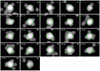 |
Fig. A.1. Images at the 0.5-2 keV energy band of all the ObsID (marked on the top left in each panel), centred on the QSO ID1. The images are binned to one-fourth of the native pixel size and smoothed using a Gaussian kernel of 3 sub-pixels. The green 2″ circle indicates the QSO centre, which was used for alignment across observations. The number of counts in the 0.5-2 keV energy band within the 2″ circles is shown on the top right corners in each panel. |
Appendix B: Lack of extended X-ray emission around the others AGN within MQN01
Figure B.1 presents the radial profiles extracted from observational data (black points) compared to those derived from the simulated PSF (red points) for other X-ray AGNs reported in Travascio et al. (2025). AGNs ID3 and ID4, located near the brightest QSO (ID1), were excluded due to their proximity, which complicates the identification of extended emission. As reported in Section 3.1, no significant extended emission is detected around these AGNs, as the normalized PSF accurately reproduces the observed profiles within the uncertainties. Beyond 4″ (corresponding to 30 kpc at z = 3.25), the uncertainties are primarily dominated by the local background. This result further validates the reliability of our analysis and the accuracy of the generated PSFs in reproducing the observational data.
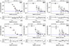 |
Fig. B.1. Radial profiles of surface counts and residuals, as shown in Figure 1, centred on the AGNs QSO ID2, ID5, and ID6 (from Travascio et al. 2025). The profiles are derived from observational data (black dots) and the simulated PSF (red dots). The top and bottom panels display the profiles in the 0.5-2 keV and 2-10 keV energy bands, respectively. |
To further test this, we estimated the ratio of net counts in the 0.5-1.5 keV energy range (where the extended emission is detected) within the 2″-3″ annulus and the 2″-radius region centred on ID1. This was then compared to the ratios for other bright X-ray point sources in the Chandra field of view (FoV), located as close as possible to ID1. Among these, the only source with a well-defined, non-elongated PSF, a high count rate, and a position near the aim point is the AGN ID2. To estimate the net counts, the background was derived from 100 large annuli around the sources, with their minimum and maximum radii chosen randomly within specific limits to minimize the influence of local background variations. By computing the median, along with the 25th and 75th percentiles, of the count ratio for ID1 and ID2, we found that the excess emission in ID1 compared to ID2 is detected at a significance level of 4.5σ (ranging between 4σ and 5σ). This calculation assumes a similar PSF for both sources, which is reasonable given their proximity.
Figure B.2 displays the 0.5-2 keV images for both the observational data (left) and the simulated PSF (right). This comparison highlights the excess counts beyond 2″ around QSO ID1, as also shown in the left panel of Figure 2.
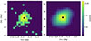 |
Fig. B.2. The same plot as in the left panel in Figure 2 (see here for further details), for the second-brightest X-ray AGN, ID2. |
Appendix C: Proof of equation (7)
Equation (7) can be derived for instance from 3.241-4 in Gradshteyn & Ryzhik (2007). However, the original source, containing the mathematical proof, is of uneasy retrieval. Furthermore, it is unclear from Gradshteyn & Ryzhik (2007) whether the formula has been proven for non-integer values of a. We therefore provide here a simple, explicit proof of equation (7), valid for all a > 0.5:
 (C.1)
(C.1)
where we used the substitution y = 1/(1 + x2), then the definition of Euler’s beta function B and finally the well known properties B(z1, z2) = Γ(z1)Γ(z2)/Γ(z1 + z2) and  . Note that for a ≤ 0.5 the integral diverges and
  is undefined, or formally infinite.
Appendix D: QSO radiation field and its impact on hot gas emission
In Section 5.2, we rapidly discover that the copious amount of ionizing photons from the central QSO cannot significantly affect the thermal X-ray emission, thus reproducing the extended X-ray emission we found. In this appendix, we report the procedure in details.
We used Cloudy (Ferland et al. 1998) to model the emission from hot CGM gas, both with and without the influence of AGN photoionization. Specifically, we simulated a coronal gas as in our fiducial model. For this test, we focused on a shell with radii 15-23 kpc, which corresponds in projection to the 2″-3″ annulus where the signal of the extended emission is the strongest (see Figure 7), and we assume a temperature and metallicity of kT = 1.8 keV and Z ≃ 0.014 Z⊙, and a gas density ⟨nH⟩ ≃ 0.4 cm−3, which is the average density value in such a shell for our fiducial beta model (see Section 5.4). The gas was placed at this distance in a shell geometry within Cloudy.
The energy injected by the central AGN was described using a spectral energy distribution (SED; panel (a) of Figure D.1) tabulated from observations ("AGN T=1.8e5 K a(ox)=-0.6 a(uv)=-2 a(x)=-1.9"), constrained to match UV [νLν(1700 Å) = 6.5 × 1046 erg s−1; Borisova et al. 2016) and X-ray νLν(2 keV) = 3.3 × 1045 erg s−1; Travascio et al. 2025) photometric measurements, adopting a X-ray power law photon-index of Γ ≈ 2.1. This setup allows us to test the potential impact of AGN photoionization on the thermal emission from the surrounding gas. We also ran an additional Cloudy simulation where the QSO SED was suppressed by 6 orders of magnitude, to simulate a condition where photoionization is negligible and CIE applies. This was done to allow for a direct comparison with the xsmekal model (which also assumes CIE) and test the dependence of the results on different codes at fixed physical assumptions.
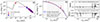 |
Fig. D.1. Impact of QSO photoionization on the thermal emission in the observed 0.5-2 keV energy band (highlighted by the shaded grey region). Panel (a) shows the SED adopted to represent the QSO radiation field, constrained by two photometric measurements (UV and X-ray; red and blue dots) for this source and by the power-law slope Γ ≈ 2.1 used to match the unfolded Chandra X-ray data (purple dots). Panel (b) compares the thermal emission spectrum predicted by the standard xsmekal model (red line) with that obtained from Cloudy simulations including QSO photoionization (see text for details). Panel (c) shows the ratio between the Cloudy model with QSO photoionization and the xsmekal model. Panel (d) displays the ratio between Cloudy thermal models computed with and without the QSO radiation field, illustrating the net impact of photoionization. |
We then reproduced the corresponding thermal emission using the xsmekal function in sherpa, adopting the same parameters as before: kT = 1.8 keV, Z = 0.014 Z⊙, and a normalization, norm2, 3, related to the gas density nH = 0.4 cm−3 via Equation (4), and adopting, in this case, a volume equal to the volume of the shell. The resulting model was rescaled to express the emission in units of νLν.
The panel (b) in Figure D.1 presents the spectra obtained for the three models described above. The Cloudy thermal models with and without QSO photoionization are shown as blue and cyan lines, respectively, while the red line corresponds to the thermal emission from the xsmekal model. The transparent grey band highlights the energy range (0.5-2 keV observed) where extended X-ray emission is detected in the Chandra data, and where we aim to identify differences between the models. The panel (c) shows the ratio between the Cloudy and xsmekal thermal models without QSO photoionization, while the bottom panel displays the ratio between the Cloudy thermal models without and with the QSO radiation field. As shown by the similarity between the blue and cyan curves, whose ratio is shown in panel (d), the impact of QSO photoionization on the thermal emission of the hot gas is negligible in this case. Additionally, the comparison between the cyan and red curves, whose ratio is shown in panel (c), shows that, even under identical physical assumptions, the predicted emission varies only marginally between different modelling codes. These small differences are negligible for our purposes and do not affect our conclusion that QSO photoionization has no significant impact on the thermal emission of the hot gas.
Appendix E: Brunt-Väisälä timescale for an isothermal β model
Following Wibking et al. (2025), we can define the Brunt-Väisälä timescale as  , where g in the gravitational field and hS is the local entropy scale-length defined as hS = (dS/dr)−1, with S = ln(Tn1 − γ). For an isothermal β-model and assuming γ = 5/3 (for a monoatomic gas), we find
 (E.1)
(E.1)
All Tables
All Figures
|
Fig. 1. Evidence of residual soft X-ray emission at < 2 keV around the brightest QSO in the MQN01 field, ID1, assuming all emission within the central 2″ is due to the AGN. This results in a conservative estimate of the extended component, which is likely non-zero even within this region. Radial profiles of surface counts centred on the QSO ID1, derived from the data (black dots) and the simulated PSF+background (red dots). Profiles are presented for two observed energy bands: 0.5–2 keV (left), 2–10 keV (middle), and 0.8–2 keV (right). Radial bins are defined such that each contains sufficient counts to achieve S/N > 3. The lower panels display residuals, expressed in units of σ, as a function of radial bin. The dashed blue line marks the background level, and the horizontal dashed lines in the residual panels correspond to the −2σ, 0σ, and +2σ levels. |
| In the text | |
|
Fig. 2. Data (left), simulated PSF (middle), and PSF-subtracted (right) images at the 0.5–2 keV energy band. Dashed red circles indicate the radial bins used for profile extraction, corresponding to the following radii: ∼2″, 2.5″, 3″, 4″, 5.5″, 8.9″, 10.3″, and 11.3″. The QSO position is marked with a black dot, and the shaded black circle represents the 2″ radius used to normalize PSF counts to the data. The annular region between 2″ and 4″ may include approximately 6 background counts. |
| In the text | |
|
Fig. 3. Smoothed soft X-ray 0.5–2.0 keV count map of the extended X-ray emission, obtained after subtracting the QSO’s PSF contribution. The filled black dot marks the QSO centre with a radius of 1″, while the transparent dot represents the inner 2″ region, where counts are used to rescale the PSF to the image. The magenta contours trace the Lyα nebula at surface brightness (SB) levels of 2.5, 4, 6, 8, 10, and 12 × 10−18 ergs−1 cm−2 arcsec−2. The red cross marks the position of the QSO companion detected with ALMA. |
| In the text | |
|
Fig. 4. Comparison of the azimuthal flux distribution of the extended Lyα and X-ray emission. (a) PSF-subtracted map of the 0.5–2 keV Chandra X-ray image after subtracting the QSO’s PSF. Red contours show the Lyα SB levels as in Figure 3. Black wedges indicate the sectors used to construct the plot in panel (b). The latter shows the azimuthal distribution of the normalized flux in each 2″–5″ sector, shown as a function of the sector’s central angle. The red curve traces the extended Lyα emission, while the black curve represents the 0.5–2 keV X-ray emission. |
| In the text | |
|
Fig. 5. Spectral evidence of excess extended X-ray emission in the soft band, relative to the expected contribution from nuclear (PSF) emission in the 2″–4″ annulus. Top panel: Energy-dependent rescaling factors derived from simulated PSFs, used to estimate the nuclear spillover contribution to the annular spectrum. Middle panel: Spectrum extracted from the central 2″ (black points; binned to at least 50 counts per bin) fitted with an AGN component (solid black line), compared to the spectrum extracted from the 2″-4″ annulus (red points; binned to at least 10 counts per bin), and the predicted nuclear spillover (dashed black line). Bottom panel: Residuals σ in the annulus after subtracting the nuclear spillover component. |
| In the text | |
|
Fig. 6. Posterior probability distributions for the simultaneous MCMC modelling of the nuclear and extended emission. Contours represent the 68%, 95%, and 99.7% confidence levels. The vertical solid red lines and the red points mark the best-fit values, which we define as the median value of the distribution of individual parameters, while the dashed red lines mark the 16th and 84th percentiles. Median and percentile values for each parameter are reported above the one-dimensional histograms along the diagonal showing the marginalized distributions for each parameter. |
| In the text | |
|
Fig. 7. Observed spectra extracted from four regions: the central 2″ aperture (top left), and the 2″–3″, 3″–5″, and 5″–8″ annuli (top right, bottom left, and bottom right, respectively). Overplotted are the best-fit models (red lines) based on the median posterior values from Table 1. The individual spectral components are shown in blue (nuclear power-law), green (thermal emission), and purple (background). Residuals in the lower sub-panels are given in units of σ. |
| In the text | |
|
Fig. 8. Redshift-dimming corrected X-ray SB profiles in the observed 0.5–2 keV band (SBX) for the extended thermal emission around QSO ID1 (red circles), obtained using an energy conversion factor (ECF) of ≃4.6 × 10⁻¹¹ erg cm−2 cnts−1 based on the best-fit values of kT = 1.8 keV and Z/Z⊙ = 0.014, and for the Spiderweb Galaxy (blue triangles) L24. A correction factor of 0.536 was applied to the Spiderweb hot halo’s SBX profile from L24 to account for differences in the redshift-dependent intrinsic energy band. The black lines show the median (solid), 16th–84th percentile (dashed) and minimum-maximum (dotted) SBX profiles of hot halos at z = 3 from the DIANOGA simulations, selected to have an average mass consistent with the estimated virial mass of the MQN01 halo (i.e. ∼3 × 10¹³ M⊙). |
| In the text | |
|
Fig. 9. Electron density (ne(r)) and pressure (Pe(r)) profiles of the hot halos in MQN01 (red), Spiderweb (blue), and DIANOGA simulations (green). The red curve shows the best-fit model for MQN01, with the shaded region indicating the 68% confidence interval. The profiles of the Spiderweb halo is from L24, while the green band represents the range of profiles extracted from DIANOGA cosmological simulations of massive halos (∼2–6 × 10¹³ M⊙) at similar redshift as MQN01 (i.e. z = 3). The dashed vertical red lines indicate the radial range between 2″ and 5″, where we observe a significant detection. |
| In the text | |
|
Fig. 10. Soft X-ray (0.5–2 keV) luminosity versus temperature kT of the ICM in massive structures across redshift. Symbols show galaxy clusters from Bulbul et al. (2019) (green squares), O’Hara et al. (2007) (orange triangles), Mittal et al. (2011) (magenta crosses), and high-redshift clusters from the literature (cyan triangles; Stanford et al. 2001; Fabian et al. 2001; Mathur & Williams 2003; Andreon & Huertas-Company 2011; Tozzi et al. 2015; Mastromarino et al. 2024). The red square marks the Spiderweb protocluster hot X-ray halo (L24), while the red circle shows the value for the X-ray halo in this work (MQN01) within a radius of 8″, respectively. The background density distributions represent the conservative MCMC posterior accounting for systematics (Section 4.3). |
| In the text | |
|
Fig. A.1. Images at the 0.5-2 keV energy band of all the ObsID (marked on the top left in each panel), centred on the QSO ID1. The images are binned to one-fourth of the native pixel size and smoothed using a Gaussian kernel of 3 sub-pixels. The green 2″ circle indicates the QSO centre, which was used for alignment across observations. The number of counts in the 0.5-2 keV energy band within the 2″ circles is shown on the top right corners in each panel. |
| In the text | |
|
Fig. B.1. Radial profiles of surface counts and residuals, as shown in Figure 1, centred on the AGNs QSO ID2, ID5, and ID6 (from Travascio et al. 2025). The profiles are derived from observational data (black dots) and the simulated PSF (red dots). The top and bottom panels display the profiles in the 0.5-2 keV and 2-10 keV energy bands, respectively. |
| In the text | |
|
Fig. B.2. The same plot as in the left panel in Figure 2 (see here for further details), for the second-brightest X-ray AGN, ID2. |
| In the text | |
|
Fig. D.1. Impact of QSO photoionization on the thermal emission in the observed 0.5-2 keV energy band (highlighted by the shaded grey region). Panel (a) shows the SED adopted to represent the QSO radiation field, constrained by two photometric measurements (UV and X-ray; red and blue dots) for this source and by the power-law slope Γ ≈ 2.1 used to match the unfolded Chandra X-ray data (purple dots). Panel (b) compares the thermal emission spectrum predicted by the standard xsmekal model (red line) with that obtained from Cloudy simulations including QSO photoionization (see text for details). Panel (c) shows the ratio between the Cloudy model with QSO photoionization and the xsmekal model. Panel (d) displays the ratio between Cloudy thermal models computed with and without the QSO radiation field, illustrating the net impact of photoionization. |
| In the text | |
Current usage metrics show cumulative count of Article Views (full-text article views including HTML views, PDF and ePub downloads, according to the available data) and Abstracts Views on Vision4Press platform.
Data correspond to usage on the plateform after 2015. The current usage metrics is available 48-96 hours after online publication and is updated daily on week days.
Initial download of the metrics may take a while.