| Issue |
A&A
Volume 709, May 2026
|
|
|---|---|---|
| Article Number | A23 | |
| Number of page(s) | 30 | |
| Section | Planets, planetary systems, and small bodies | |
| DOI | https://doi.org/10.1051/0004-6361/202558343 | |
| Published online | 28 April 2026 | |
Confirmation of the hot super-Neptune TOI-672 b with NIRPS and HARPS
Insights into the Neptunian desert around M dwarfs
1
Univ. Grenoble Alpes, CNRS, IPAG,
38000
Grenoble,
France
2
Department of Physics & Astronomy, McMaster University,
1280 Main St W,
Hamilton,
ON,
L8S 4L8,
Canada
3
Department of Physics, The University of Warwick,
Gibbet Hill Road,
Coventry,
CV4 7AL,
UK
4
Observatoire de Genève, Département d’Astronomie, Université de Genève,
Chemin Pegasi 51,
1290
Versoix,
Switzerland
5
Institut Trottier de recherche sur les exoplanètes, Département de Physique, Université de Montréal,
Montréal,
Québec,
Canada
6
Light Bridges S.L., Observatorio del Teide, Carretera del Observatorio,
s/n Guimar,
38500
Tenerife,
Canarias,
Spain
7
Instituto de Astrofísica de Canarias (IAC),
Calle Vía Láctea s/n,
38205
La Laguna,
Tenerife,
Spain
8
Departamento de Astrofísica, Universidad de La Laguna (ULL),
38206
La Laguna,
Tenerife,
Spain
9
Observatoire du Mont-Mégantic,
Québec,
Canada
10
Instituto de Astrofísica e Ciências do Espaço, Universidade do Porto,
CAUP, Rua das Estrelas,
4150-762
Porto,
Portugal
11
Departamento de Física e Astronomia, Faculdade de Ciências, Universidade do Porto,
Rua do Campo Alegre,
4169-007
Porto,
Portugal
12
Department of Earth, Planetary, and Space Sciences, University of California,
Los Angeles,
CA
90095,
USA
13
Department of Physics, University of Toronto,
Toronto,
ON
M5S 3H4,
Canada
14
Departamento de Física Teórica e Experimental, Universidade Federal do Rio Grande do Norte,
Campus Universitário,
Natal,
RN,
59072-970,
Brazil
15
Department of Physics, McGill University,
3600 rue University,
Montréal,
QC,
H3A 2T8,
Canada
16
Department of Earth & Planetary Sciences, McGill University,
3450 rue University,
Montréal,
QC,
H3A 0E8,
Canada
17
Centre Vie dans l’Univers, Faculté des sciences de l’Université de Genève,
Quai Ernest-Ansermet 30,
1205
Geneva,
Switzerland
18
European Southern Observatory (ESO),
Karl-Schwarzschild-Str. 2,
85748
Garching bei München,
Germany
19
Space Research and Planetary Sciences, Physics Institute, University of Bern,
Gesellschaftsstrasse 6,
3012
Bern,
Switzerland
20
Consejo Superior de Investigaciones Científicas (CSIC),
28006
Madrid,
Spain
21
Bishop’s University, Dept of Physics and Astronomy,
Johnson-104E, 2600 College Street,
Sherbrooke,
QC,
J1M 1Z7,
Canada
22
Department of Physics, Engineering Physics, and Astronomy, Queen’s University,
99 University Avenue,
Kingston,
ON
K7L 3N6,
Canada
23
Department of Physics and Space Science, Royal Military College of Canada,
13 General Crerar Cres.,
Kingston,
ON
K7P 2M3,
Canada
24
Center for astrophysics | Harvard & Smithsonian,
60 Garden Street,
Cambridge,
MA
02138,
USA
25
Centro de Astrobiología (CAB), CSIC-INTA,
Camino Bajo del Castillo s/n,
28692,
Villanueva de la Cañada (Madrid),
Spain
26
Boyce Research Initiatives and Education Foundation,
3540 Carleton St.,
San Diego,
CA
92106,
USA
27
El Sauce Observatory,
Coquimbo Province,
Chile
28
European Southern Observatory (ESO),
Av. Alonso de Cordova 3107,
Casilla
19001,
Santiago de Chile,
Chile
29
Department of Astronomy, Westlake University,
Hangzhou
310030,
Zhejiang Province,
PR China
30
University Observatory, Faculty of Physics, Ludwig-Maximilians-Universität München,
Scheinerstr. 1,
81679
Munich,
Germany
31
Department of Physics and Astronomy, University of Waterloo,
200 University W,
Waterloo,
ON
N2L 3G1,
Canada
32
Perth Exoplanet Survey Telescope,
Perth,
Western Australia,
Australia
33
American Association of Variable Star Observers,
Cambridge,
USA
★ Corresponding author: This email address is being protected from spambots. You need JavaScript enabled to view it.
Received:
1
December
2025
Accepted:
10
March
2026
Abstract
The Neptunian desert is a distinct lack of Neptune-sized planets at short orbital periods, purportedly carved by photoevaporation and tidal circularisation following high-eccentricity migration. Constraining these processes and how they vary across different hoststar spectral types requires detailed characterisation of the planets in the desert and around its boundaries. In this study, we confirm the planetary nature of a massive super-Neptune identified by TESS around the M0 dwarf TOI-672. We analysed photometry from TESS and ExTrA and precise radial velocity measurements taken with the recently commissioned Near-InfraRed Planet Searcher (NIRPS) and HARPS spectrographs. We measured a planetary orbital period of 3.634 days, a radius of 5.31−0.26+0.24 R⊕, and mass of 50.9−4.4+4.5 M⊕. Our findings place TOI-672 b within the Neptunian ridge, a pile-up of planets from 3-5 days at the Neptunian desert boundary. We used a novel approach to determine the desert boundaries in period-radius space and instellation-radius space, and for the first time, we compared the Neptunian desert boundaries for planets orbiting FGK versus M dwarf stars. We determined that the boundary ridge shifts slightly inwards from 3.3 ± 1.4 days for FGK host stars to 2.2 ± 1.0 days for M dwarf host stars. Statistically, these values do not significantly differ from each other, and the shift to shorter periods for M dwarf planets is smaller than what theoretical photoevaporation models predict. We also find that TOI-672 b is a single-planet system within the sensitivity limits of our RV and TTV datasets.
Key words: techniques: radial velocities / planets and satellites: general / planets and satellites: individual: TOI-672 b
© The Authors 2026
 Open Access article, published by EDP Sciences, under the terms of the Creative Commons Attribution License (https://creativecommons.org/licenses/by/4.0), which permits unrestricted use, distribution, and reproduction in any medium, provided the original work is properly cited.
This article is published in open access under the Subscribe to Open model. This email address is being protected from spambots. You need JavaScript enabled to view it. to support open access publication.
1 Introduction
A prominent feature in the exoplanet population is the ‘Neptune desert’, a significant lack of Neptune-sized exoplanets (approximately 2-10R⊕ and 6-250 M⊕) on short orbital periods (≲3 days), shown in Fig. 1. The existence of the Neptune desert was noted by many as the population of exoplanets grew (see e.g. Szabó & Kiss 2011; Beaugé & Nesvorny 2013; Lundkvist et al. 2016; Mazeh et al. 2016) and given several names (e.g. the ‘sub-Jovian Pampas’, a ‘hot-super-Earth desert’, and the ‘short-period Neptunian desert’).
The boundaries of the Neptunian desert and the planet populations that underpin it have been the subject of a number of studies. Perhaps the most prominent is the work by Mazeh et al. (2016), which followed earlier work by Szabó & Kiss (2011) but featured a larger sample of planets. Mazeh et al. (2016) defined empirical boundaries for the desert using linear slopes to designate the upper and lower boundaries in the period-radius and period-mass spaces (shown in Fig. 1). The analysis in that work used a mix of known planets with masses reported in the exoplanet encyclopedia1 and Kepler planet candidates, with no corrections for detection bias. These boundaries have since become the de facto location of the desert in many works, with extrapolation of the boundaries (beyond the period range they were calculated for) to intersect at an orbital period of ∼10 days.
Recently, there have been several studies devoted to updating the desert boundaries and exploring nearby regions (e.g. Deeg et al. 2023; Szabó et al. 2023; Castro-González et al. 2024; Magliano et al. 2024; Peláez-Torres et al. 2024). It has been proposed that there is a Neptunian ‘savanna’ (Bourrier et al. 2023), a somewhat milder deficit of Neptunian-sized planets (∼4-8 R⊕) at longer periods (≳5 days). Castro-González et al. (2024) used the Kepler DR25 data to derive new boundaries, with planets weighted according to transit and detection probabilities (i.e. correcting for observational biases). In period-radius space, they used a kernel density estimation on the weighted individual planets to define the desert boundaries as the region with no planets at the 3σ level. Similar to Mazeh et al. (2016), Castro-González et al. (2024) drew upper and lower boundaries but identified an over-density of planets between ∼3-6 days, subsequently named the ‘ridge’, that cuts off the tip of the desert and separates it from the savanna (see Fig. 1).
There is a consensus that the Neptune desert is not the result of observational biases, as transit and radial velocity surveys are highly sensitive to Neptune-like planets on short orbital periods. The prevailing theory is that the Neptune desert is sculpted by several processes. The upper boundary is predominantly shaped by high-eccentricity migration of large planets, where gravitational interactions kick the planet onto an eccentric orbit before being tidally circularised near periastron (Mat-sakos & Königl 2016). Planets with larger masses can tidally circularise closer to their stars without experiencing tidal disruption, producing a negative slope for the upper boundary in period-radius and period-mass spaces (Owen & Lai 2018). The lower boundary is thought to be predominantly shaped by photoevaporation, wherein Neptune-sized planets are stripped of their H2-He envelopes to become super-Earths due to XUV irradiation from their host stars (e.g. Owen & Lai 2018; Ionov et al. 2018; Owen 2019; Vissapragada et al. 2022; Thorngren et al. 2023). The efficiency of mass-loss increases as the orbital period decreases, producing a positive slope for the lower boundary in period-radius and period-mass spaces. Finally, the current understanding of planets within the ridge is that they may be a product of late dynamical migration, with elevated eccentricities and misaligned orbits (Castro-González et al. 2024).
It follows from the physical mechanisms purported to carve out the Neptunian desert that its boundaries do not solely depend on the properties of the planets but also on those of their host stars. The orbital period has been used as an important parameter in many Neptunian desert studies, as it is readily available with exceptionally high precision for many planets. However, a planet at a given orbital period around an F star, for example, is going to be more heavily irradiated than a planet at the same orbital period around an M dwarf. With this in mind, some studies have moved away from period space and instead use alternative dimensions, such as instellation, planetary equilibrium temperature, and lifetime X-ray irradiation (e.g. Lundkvist et al. 2016; McDonald et al. 2019; Burt et al. 2020; Kanodia et al. 2021; Persson et al. 2022; Powers et al. 2023; Magliano et al. 2024). Szabó & Kálmán (2019) and Szabó et al. (2023) showed that the Neptunian desert boundaries depend on stellar parameters, including (in order of decreasing significance) effective temperature, metallicity, log g, and stellar mass. In particular, Szabó & Kálmán (2019) revealed, for Neptune-sized planets in the desert region, an increase in the occurrence of close-in planets with decreasing stellar effective temperature. Approximately 60% of planets with host stars colder than 5600 K have orbital periods shorter than ten days, but for host stars hotter than 5600 K, this drops to ∼10%. In short, in this particular region, cooler stars have a higher proportion of short-period planets compared to hotter stars. Consequently, the Neptunian desert boundaries derived by Mazeh et al. (2016) and Castro-González et al. (2024) in the period-radius space may not be the same when considering planets around different types of host stars. This has been highlighted by Kanodia et al. (2021) and Powers et al. (2023), who translated the Mazeh et al. (2016) desert boundaries into insolation-radius space for different stellar types. Specifically, the boundaries move towards lower instellations for M dwarf hosts compared to FGKs, leading to the question of whether an M dwarf planet is in the desert or not. Indeed, Hallatt & Lee (2022) predict that the opening of the Neptunian desert (i.e. where the upper and lower boundaries intersect) in period-radius space should shift to shorter orbital periods around M dwarfs, beginning at ∼0.7 days around 0.5 M⊙ stars and ∼1.5 days around 0.8 M⊙ stars, compared to ∼3 days around 1 M⊙ stars. They predict that a shift in the opening and the width of the Neptunian desert would be the most evident when comparing the planet sample around M dwarfs against solar-type stars.
Investigation of the Neptunian desert thus far has been biased towards planetary systems around Sun-like stars since the Kepler primary mission, the source of a large proportion of exoplanet discoveries, was focused on the search for Earth-sized planets around FGK stars. Additionally, M dwarfs are typically harder to observe because they are fainter. This is especially significant for precise radial velocity (RV) follow-up studies aiming to confirm the nature of planetary candidates and obtain their masses, as observations of this kind are typically conducted at visible wavelengths. Consequently, samples used for studying the Neptunian desert have included comparatively few planets around M dwarfs compared to FGK stars. However, there are now a number of spectrographs that are particularly suited to characterising planets around M dwarfs. Optical spectrographs that operate below 1 μm and are mounted on 8m-class telescopes (e.g. ESPRESSO (Pepe et al. 2021) and MAROON-X (Seifahrt et al. 2018) are able to collect more light and potentially reach these fainter targets. Alternatively, M dwarfs are brighter in the red optical and near-infrared (NIR), thus motivating the push towards the commissioning of NIR spectrographs such as CARMENES (Quirrenbach et al. 2016), IRD (Tamura et al. 2012), HPF (Mahadevan et al. 2012), SPIRou (Donati et al. 2020), and the Near-InfraRed Planet Searcher (NIRPS) (Bouchy et al. 2025; Artigau et al. 2024a), the recently commissioned NIR arm of the High Accuracy Radial velocity Planet Searcher (HARPS; Pepe et al. 2002; Mayor et al. 2003).
Here we present the confirmation of a hot Neptune orbiting an M0 dwarf star, TOI-672 b, and the precise characterisation of its mass using the NIRPS and HARPS RV spectrographs. These data were obtained under the NIRPS Guaranteed Time Observations (GTO) program. We refine the planetary orbital and physical parameters and confirm its position in the Neptunian ridge, making it an interesting test case for formation and evolution models of Neptunian desert planets.
Our paper is laid out as follows. In Section 2, we describe our photometric and spectroscopic observations of TOI-672. We then report stellar parameters, including elemental abundances of the host star in Section 3. In Section 4, we describe the joint fit model to the RV and transit data. In Section 5, we discuss the results of our joint fit and the nature of TOI-672 b, and we predict its composition and look at its photoevaporation history. We also calculate the sensitivity of our RV data in relation to detecting additional planets in the system, and we search for transit timing variations. Finally, we present an analysis of the Neptunian desert boundaries around M dwarf planet hosts in comparison to FGK hosts in Section 6. We put forward our conclusions in Section 7.
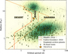 |
Fig. 1 Period-radius diagram showing TOI-672 b (yellow star) against the known planet population (light grey dots). Data of the known planet population are from the NASA exoplanet archive2, and only those with periods and radii determined to better than 4σ are shown. The background is also shaded according to this population. Planets around M dwarf hosts are highlighted (as green circles with a black outline, cut on Teff < 3900K, M*, R* < 0.6 M⊙, R⊙). The Neptunian desert boundaries derived by Mazeh et al. (2016) (orange line) and Castro-González et al. (2024) (red line) are shown. The desert, ridge, and savanna, as defined by Castro-González et al. (2024), are labelled, and the higher-period cut-off of the ridge is shown (dashed red line). |
2 Observations and previous validation
2.1 TESS photometry
The TOI-672 system (Table 1) was observed in Transiting Exoplanet Survey Satellite (TESS) Sectors 9 (28 February-26 March 2019), 10 (26 March-22 April 2019), 36 (07 March-2 April 2021), and 63 (10 March-6 April 2023), all on Camera 2 with a 2-min cadence. TOI-672.01 (now TOI-672b) was detected by the Transiting Planet Searcher (TPS, Jenkins 2002; Jenkins et al. 2010) using the light curves from the TESS Science Processing Operations Center (SPOC) pipeline at the NASA Ames Research Centre (Jenkins et al. 2016; Caldwell et al. 2020), as well as being detected by the MIT Quick-Look Pipeline (QLP, Huang et al. 2020), and became a TESS Object of Interest (TOI) on 7 May 2019. The transiting planet parameters given in the TOI catalog3 were updated after the Sector 36 then Sector 63 observations, and as of 3 Dec 2023 gave a reference mid-transit time of 2 458 546.4800 ± 0.0003 BJD, a period of 3.633574 ± 0.000003 d, a transit duration of 1.78 ± 0.05 hours, and a depth of 8668 ± 124 ppm (parts per million).
The data products are available on the Mikulski Archive for Space Telescopes (MAST4) and were produced by the TESS SPOC. We downloaded the publicly available photometry provided by the SPOC pipeline. In our main fit (Section 4) we use the Presearch Data Conditioning Simple Aperture Photometry (PDCSAP), which is the product of removing common trends and artefacts from the Simple Aperture Photometry (SAP) by the SPOC Presearch Data Conditioning (PDC) algorithm (Twicken et al. 2010; Smith et al. 2012; Stumpe et al. 2012, 2014). We remove all data points with a non-zero quality flag, and show the median-normalised PDCSAP flux in Fig. 2. The PDCSAP photometry preserves stellar activity, which we will detrend as described in Section 4.1; the detrended photometry is shown in Fig. 2 and phase folded in Fig. 3.
Details for the TOI-672 system.
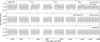 |
Fig. 2 TESS photometry for TOI-672 covering Sectors 9, 10, 36, and 63 (left to right, chronologically). The data are described in Section 2.1, and the fit to these data is described in Section 4.1. Top panel : PDCSAP flux (grey circles) and the GP model (green line) used for detrending. Middle panel : detrended flux after the GP model is subtracted and with the transit model shown (orange line). Bottom panel : residuals left after the GP and transit models are subtracted from the photometry. |
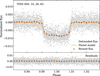 |
Fig. 3 Top panel : detrended TESS photometry for TOI-672 from all sectors (grey circles, binned as dark brown circles) phase folded on the best-fit planetary period and with the transit model shown (orange line). Bottom panel: residuals after the GP and planet models are subtracted from the photometry. |
2.2 Ground-based photometry
The TESS pixel scale is ∼21" per pixel, and while the SAP aperture for TOI-672 is variable, it is typically three pixels (∼1′) on a side. We show the apertures for each sector in Fig. A.1. Multiple stars can blend in an aperture of this size which can cause confusion in the source of the transit detection, and dilute the transit depth. Indeed, looking for other nearby stars within several magnitudes of TOI-672, there are two faint Gaia sources that fall within the aperture (with ∆Gmag = 3.21,4.64), and a bright neighbouring source (∆Gmag = −0.34) located 53.17" to the north west (see Fig. A.1). The SAP photometry includes a dilution parameter (a ratio of the target flux to total flux in the aperture), which varies from 0.95 to 0.98 depending on sector.
All light curve data described below are available on the EXOFOP-TESS website5. We did not include these observations in our joint fit, with the exception of one transit from ExTrA (see Section 4), but we do use their individual mid-transit times when conducting our Transit Timing Variations (TTV) search (see Section 5.5). The light curves are depicted in Fig. A.2. A summary of all photometric transits, and whether they were used in the joint fit and for the TTV search, can be found in Table A.1.
2.2.1 TFOP photometry
To attempt to determine the true source of the TESS detection, ground-based time-series follow-up photometry of the field around TOI-672 were obtained as part of the TESS Followup Observing Program (TFOP; Collins 2019)6. The majority of these observations are presented in the validation of this target (detailed in Section 2.3; Mistry et al. 2023), so we do not describe them here except as a brief summary.
Two full transits were observed from the Las Cumbres Observatory Global Telescope (LCOGT; Brown et al. 2013) network nodes on 2019 May 11 (at the Cerro Tololo Inter-American Observatory, CTIO, in Chile) and 2020 March 19 (at the Siding Spring Observatory, SSO, near Coonabarabran, Australia). A partial and a full transit were observed on UTC 2019 May 11 and 2020 February 01, respectively, from the Evans 0.36 m telescope at El Sauce Observatory in Coquimbo Province, Chile. A full transit was observed on 2019 May 26 using the Perth Exoplanet Survey Telescope (PEST), located near Perth, Australia. One additional transit, not described by Mistry et al. (2023), was made on June 14, 2022, using a 17" telescope (CDK17) installed in Chile (Deep Sky Chile) with a Cousin R filter. The light curve was calculated using the HOPS software from the ExoClock collaboration (Kokori et al. 2022).
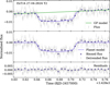 |
Fig. 4 ExTrA photometry for TOI-672 from the night of 27 April 2024 using Telescope 2 (T2). The data are described in Section 2.2.2, and the fit to these data is described in Section 4.2. Top panel : extracted photometry (grey circles, binned as dark purple circles) and the GP model used to detrend it (green line). Middle panel : detrended photometry showing the transit model (purple line). Bottom panel residuals after the GP and transit models are subtracted from the photometry. |
2.2.2 ExTrA photometry
We supplemented the existing TFOP photometry with additional ground-based transit observations over many transit windows to aid in our TTV search, and to expand the baseline of transit observations to improve constraints on the orbital period of the planet. We used ExTrA (Exoplanets in Transits and their Atmospheres, Bonfils et al. 2015), a low-resolution NIR (0.85-1.55 μm) multi-object spectrograph fed by three 60-cm telescopes located at La Silla Observatory in Chile. We used 8" diameter aperture fibres and the low-resolution mode (R ~ 20) of the spectrograph, with an exposure time of 60 seconds. We positioned five fibres in the focal plane of each telescope to isolate light from the target and four comparison stars. The resulting ExTrA data were analysed using custom data reduction software (Cointepas et al. 2021).
We observed transits of TOI-672 b using one, two, or all three of the ExTrA telescopes (T1, T2, and T3, respectively) on a total of 12 nights from 2019 to 2024: 22 April 2021 (T2, T3); 14 May 2021 (T2, T3); 3 February 2022 (T1, T2, T3); 4 March 2022 (T1, T2, T3); 6 April 2022 (T2, T3); 24 April 2022 (T2, T3); 16 February 2023 (T1, T2, T3); 28 March 2023 (T1, T2, T3); 8 April 2023 (T1, T2, T3); 18 March 2024 (T1, T2); 29 March 2024 (T1, T2); and 27 April 2024 (T2). Most ExTrA photometry was not used in the joint fit (see Section 4), with the exception of the most recent observation from 27 April 2024 using T2 as this extended the overall baseline of the photometry. This particular observation is shown in Fig. 4. The remaining photometry (a few nights excepted due to the lack of, or poor quality of, the transit ingress) was used in the aforementioned TTV search (see Section 5.5) and is shown in Fig. A.3.
2.3 Previous validation
We note that TOI-672 b was previously validated by the Validation of Transiting Exoplanets using Statistical tools project (VaTEST; Mistry et al. 2023) based on high-resolution imaging; ground-based photometry; and TESS Sectors 9, 10, and 36 but not the most recent Sector 63 data. In summary, TOI-672 b passed multiple diagnostic tests and was statistically validated using the tool TRICERATOPS (Giacalone et al. 2021). The high-resolution imaging from the Zorro instrument on Gemini-S shows no close-in contaminating stellar companions, and the ground-based follow-up (which includes the LCOGT, Evans, and PEST observations described above) shows the transit event occurring on the target star. The TESS data from Sectors 9, 10, and 36 were fit with a transit model using Juliet (Espinoza et al. 2019) to obtain an orbital period of 3.633575 ± 0.000001 days; a radius of  R⊕, assuming a stellar radius of 0.54 ± 0.02 R⊙; an impact parameter of
  ; and an inclination of
  .
.
2.4 NIRPS and HARPS spectroscopy
We obtained simultaneous radial velocity measurements of TOI-672 with the NIRPS (Bouchy et al. 2025; Artigau et al. 2024a) and HARPS (Pepe et al. 2002; Mayor et al. 2003) spectrographs. Both instruments are mounted on the ESO 3.6-m telescope at the La Silla Observatory in Chile and can be operated simultaneously through the use of a VIS-NIR dichroic.
Operating in the optical, HARPS covers a wavelength range of 0.38-0.69μm. It has two modes corresponding to two different sets of fibres: a high accuracy mode (HAM, R = 115 000) and a high efficiency mode (EGGS, R = 80000). While EGGS is lower in resolution, it uses a fibre with a projected aperture of 1.4" on sky (a fibre diameter of 100μm), which is bigger than the 1.0" aperture (70 μm diameter) of the HAM fibre, and therefore it gains in flux collection, which is important when observing fainter M dwarf targets. HARPS was used in EGGS mode with an exposure time of 1200 s.
The recently commissioned NIR, adaptive optics-assisted spectrograph NIRPS is intended to complement HARPS as its “red arm”, and began science operations on 1 April 2023. It covers a wavelength of 0.97-1.92μm across the YJH bands. NIRPS also has two observing modes: a high accuracy (HA) mode using a 0.4" fibre with a resolution of 88 000, and a high efficiency (HE) mode using a bigger fibre of 0.9" at the expense of a lower spectral resolution of 75 200. NIRPS was used in HE mode with two back-to-back exposures of 600 s, which are then binned per night. This is due to a practical limit on the integration time for NIRPS; there is no benefit to integrating longer than the point at where dark current surpasses the readout noise, which occurs at an integration time of approximately 900 s. Longer total integrations are instead achieved by taking multiple exposures and combining them (Artigau et al. 2024b).
Our observations of TOI-672 were obtained through the NIRPS Guaranteed Time Observations (GTO) program, which began in April 2023 and was allocated 725 nights over five years. The program is split into three primary sub-programs, each with their own distinct science cases (Bouchy et al. 2025). This work was performed under Work Package 2 (WP2), which is performing mass measurements of known planets around M dwarfs (Parc et al. 2025; Frensch et al. 2026; Weisserman et al. 2026). We specifically observed TOI-672 as part of the “Deep Search” programme. RV follow-up makes us sensitive to more planets than those known from lightcurves alone. Deep Search prioritises the follow-up of targets with an a priori higher likelihood of harbouring these extra planets, and additionally prioritises systems where there is a higher chance of later seeing these planets in transit too.
We observed TOI-672 with NIRPS and HARPS simultaneously over a total of 24 nights between April 2023 and July 2024. There were nights when, for various reasons, only one instrument managed to successfully observe the target, namely, 8 Apr. 2023 (NIRPS only); 24 Jun. 2023 (HARPS only); 27 and 30 May, 1 and 29 Jun., and 1 and 3 Jul. 2024 (NIRPS only). On the night of 10 Apr. 2023, the target was observed twice by both HARPS and NIRPS (i.e. 2 HARPS spectra and 4 NIRPS spectra were obtained). Additionally, two observations were spuriously made in HARPS HAM on the nights of 29 Jun. 2024 and 1 Jul. 2024; we do not include these in our analysis as they would require treatment as a separate instrument and the RV precision is comparatively worse. No observations were obtained when the planet was in transit, so our RVs are not affected by the Rossiter-McLaughlin effect. In total, we obtained 48 usable spectra from NIRPS, which are binned nightly to produce 23 RV measurements. 18 HARPS spectra were obtained, but one from the night of 14 Jul. 2024 only had a signal-to-noise ratio (S/N) of 2 at 550 nm and was thus discarded, resulting in 17 HARPS RV measurements. The median S/N for the NIRPS at 1600 nm is 40.0; it is 9.7 for HARPS at 550nm.
The NIRPS GTO team currently uses two independent pipelines to reduce NIRPS data and produce 2D spectra. The first is an ESO pipeline based on the ESPRESSO pipeline (Pepe et al. 2021), which has been adapted to correct for the telluric absorption lines and OH emission lines (Allart et al. 2022; Bouchy et al. 2025; Srivastava et al. 2026). The second is the APERO pipeline initially created to reduce SPIRou data (Cook et al. 2022), another NIR spectrograph mounted on the Canada-France-Hawaii Telescope and with similar specifications to NIRPS. Our NIRPS data presented herein were reduced using the ESO pipeline. We reduced our HARPS data using the standard offline HARPS data reduction pipeline (ESO DRS 3.5).
While the pipelines above try and correct for contamination from telluric absorption and in the NIR spectra, this is not always perfect, particularly at times where the systematic velocity of the star is close to the barycentric Earth radial velocity (BERV). Here, the stellar and telluric lines overlap, adversely affecting the correction. For this system, this “BERV crossing” occurs between approximately 3030-3075 BJD-2 457 000 (highlighted in Fig. 5). This event reoccurs every 365 days, but our second year of observations do not start until after the BERV crossing for that year has already occurred. We attempt to mitigate the effect of the BERV crossing following the method of Srivastava et al. (2026), where we mask pixels across all observations that exhibit variations in flux beyond a certain σ threshold relative to the median stellar spectrum. This, however, does not produce a meaningful difference to either the individual RV values, nor in the rms of the RVs, at several attempted sigma thresholds (down to 2.5σ). Therefore, we do not use these masked spectra, and instead remove the effects of the BERV crossing event with a GP on the extracted RVs, which is described in Section 4.3. We note other methods for correcting for the BERV crossing have been explored in Parc et al. (2025) and Frensch et al. (2026).
After the 2D spectra is produced, RVs are then extracted. Again, precision radial velocities in the near infrared are affected by telluric absorption residuals that produce time-dependent effects on line profiles. The data-driven Line-By-Line (LBL) method (Artigau et al. 2022) was specifically developed to provide resilience to this by operating over individual spectral lines, allowing for identification and removal of these spectral outliers that would otherwise bias the measurement of the radial velocity. We thus extracted both NIRPS and HARPS RVs using LBL (version 0.65.006). Due to the relatively few observations of TOI-672, rather than constructing the template spectra from the combined spectra of this target, we instead use “friend” templates. The ‘friend’ is a different bright star with a spectral type and rotational velocity similar to the target (here TOI-672), but it has had many observations using the same spectrograph and thus has a template of sufficient S/N and excellent rejection of telluric features. For NIRPS RV extraction, we used NIRPS observations of GJ2066 (Teff = 3550 ± 157 K and log g = 4.788 ± 0.006 cgs from TICv8, Stassun et al. (2019) to construct the friend template. For HARPS RV extraction, we use HARPS observations of TOI-776 (Teff = 3725 ± 60 K; log g = 4.8 ± 0.1 cgs; [Fe/H] = −0.21 ± 0.08 dex; and v sin i = 2.2 ± 1.0 kms−1, Fridlund et al. 2024) to construct the friend template.
The LBL method also measures a number of activity indicators, including the Full-Width at Half-Maximum (FWHM) and contrast, which are both also commonly measured using the Cross Correlation Function (CCF) method. It also provides two additional indicators, the differential line width (dLW) and differential temperature of the star (dTemp), which are explained by Artigau et al. (2022) and Artigau et al. (2024b), respectively. The activity indicators and stellar rotation are discussed in Section 3.3.
The resultant NIRPS and HARPS LBL time-series data can be found in Tables B.1 and B.3, respectively. The RVs are shown in Figs. 5 and 6. Lomb-Scargle periodograms (Lomb 1976; Scargle 1982; Press & Rybicki 1989) of the RVs and activity indicators are shown in Fig. B.1.
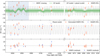 |
Fig. 5 Data from NIRPS and HARPS for TOI-672. The data are described in Section 2.4, and the fit to these data are described in Section 4.3. Top panel : NIRPS RVs (red triangles), the GP model fit to the NIRPS RVs (green line, with the one and two standard deviations of the fit shaded), and the combined GP and planet model (grey line). The BERV crossing event described in Section 2.4 is shaded in blue. Middle panel : both sets of RVs. Here, NIRPS has been detrended with a GP, and HARPS (blue circles) has no detrending. The planet-only model is shown with a grey line. Bottom panel : radial velocity residuals after the GP and planet models have been subtracted. |
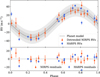 |
Fig. 6 Top panel : detrended NIRPS and HARPS RVs (red triangles and blue circles, respectively) phase-folded on the best-fit planetary period. The planet model is shown with a grey line, while the grey shading represents the one (darker) and two (lighter) standard deviations of the fit. Bottom panel : radial velocity residuals after the GP and planet model have been subtracted. |
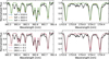 |
Fig. 7 Normalised NIRPS spectrum of TOI-672 (black line) compared to PHOENIX ACES stellar models (coloured lines). The models are described in Section 3.1.1. Top row : models with a fixed metallicity of −0.3 dex and Teff values of 3720 (blue), 3820 (orange), and 3920 (green) K for two spectral regions. Bottom row: same regions, but we show models with a fixed Teff of 3820 K and metallicity values of −0.5 (red), −0.3 (purple), and −0.1 (brown) dex. For strong spectral lines, we performed χ2 minimisation between the NIRPS spectrum and a grid of PHOENIX ACES models, finding Teff = 3810 ± 33 K and [M/H]=−0.3 ± 0.1 dex. |
3 Stellar characterisation
3.1 Stellar parameters
Here we derive parameters for the host star TOI-672 using a variety of techniques. These are reported in Table 2.
3.1.1 From the NIRPS spectra
We first co-added the telluric-corrected NIRPS spectra from APERO into a single high-resolution template of S/N∼280 to derive spectroscopic parameters following the methodology of Jahandar et al. (2024, 2025). We derived the effective temperature, Teff, and overall metallicity, [M/H], by fitting a selection of strong spectral lines through χ2 minimisation, using a grid of PHOENIX ACES stellar models (Husser et al. 2013) interpolated to log g = 4.75 and convolved to the spectral resolution of NIRPS (shown in Fig. 7). We note that we used a slightly different log g than in 3.1.3, but that a variation in log g of 0.2 dex has negligible effect on the spectral analysis. We obtained Teff = 3810 ± 33 K and [M/H] = −0.3 ± 0.1 dex. We used these values as starting points in our subsequent analysis of the stellar abundances (see Section 3.2), which we ultimately used to measure the true overall metallicity, [M/H]. To validate our spectroscopically derived Teff, we also derived Teff using the empirical M dwarf Teff -colour relation from Mann et al. (2015). We used the Gaia GBP and GRP magnitudes to derive Teff = 3783 ± 52 K, which agrees with the value measured from our NIRPS spectra.
3.1.2 From the HARPS spectra
We then used the co-added spectra from HARPS to derive Teff and [Fe/H] with the machine learning code ODUSSEAS7 (Antoniadis-Karnavas et al. 2020, 2024). This code measures the pseudo-equivalent width of more than 4000 lines in the optical spectra which are then used as input in the machine learning model trained with a reference sample of 47 M dwarfs observed with HARPS. The reference values of Teff for those stars come from interferometric calibrations (Khata et al. 2021), whereas the [Fe/H] comes from photometric calibrations in binaries (Neves et al. 2012). We obtained Teff = 3751 ± 94 K, which is in good agreement with the above mentioned values, and [Fe/H] = 0.09 ± 0.11 dex, which is higher than the value obtained from NIRPS spectra (see Section 3.2). Given that the chemical abundances are derived from the NIRPS spectra, we adopt the stellar parameters obtained with the NIRPS spectra as well.
Stellar parameters and chemical abundances of the host star TOI-672.
3.1.3 From empirical M dwarf relations
We use the empirical M dwarf radius-luminosity relation from Mann et al. (2015) to derive a stellar radius of
R* = 0.54 ± 0.02R⊙ from the star’s absolute Ks-band magnitude. However, Tayar et al. (2022) argue that there is a systematic uncertainty floor that should be accounted for, with the recommendation to add a 4.2% error in quadrature with the formal uncertainty on stellar radius. This results in R* = 0.54 ± 0.03 R⊙. Similarly, we use the empirical M dwarf mass-luminosity relation from Mann et al. (2019) to derive a stellar mass of M* = 0.54 ± 0.01 M⊙ based on the star’s absolute Ks-band magnitude. Again, we add a systematic error in quadrature with this value as recommended by Tayar et al. (2022); for stellar mass this is 5%. This results in M* = 0.54 ± 0.03 M⊙. We then use the stellar mass and radius to derive the stellar surface gravity, log g = 4.70 ± 0.03 cgs. We can also use the stellar radius and effective temperature to derive the bolometric luminosity Lbol = 0.056 ± 0.004 Lbol,⊙.
3.1.4 From SED fitting
As an alternate approach to determining the bolometric luminosity and stellar radius and mass, we built the spectral energy distribution (SED) using flux densities from several broadband photometric surveys: GBP, G, and GRP from the Gaia mission (Gaia Collaboration 2023); B and V from APASS (Henden et al. 2015); B and I from the Johnson UBVRI system (Bessell 1990); J, H, and Ks from 2MASS (Skrutskie et al. 2006); g′, r′, i′, and z′ from the SDSS system (Alam et al. 2015); and W1 -W4 from WISE (Wright et al. 2010). All magnitude values are given in Table 1. The SED fitting was carried out with the Virtual Observatory Spectral Analyzer (VOSA) (Bayo et al. 2008). Synthetic SEDs were generated from several atmospheric model grids, including BT-Settl (Allard et al. 2012), Kurucz (Kurucz 1993), and Castelli & Kurucz (Castelli & Kurucz 2003). The bestfitting model was a BT-Settl atmosphere with Teff = 3600 K, [M/H] = −0.5 dex, and log g = 5.0 cm s−2. VOSA applies a χ2 minimisation approach to match the theoretical SED to the observed photometry, accounting for the observed and model fluxes, their associated uncertainties, the number of photometric points, the adopted input parameters, and the object’s radius and distance. The resulting fit is presented in Fig. C.1. We integrated the observed SED to obtain the bolometric luminosity, Lbol = 0.04799 ± 0.00022L⊙. The stellar radius, R* = 0.563 ± 0.016R⊙, was then derived using the Stefan-Boltzmann relation  . Finally, the stellar mass was estimated as M* = 0.570 ± 0.021 M⊙ using Equation (6) from Schweitzer et al. (2019). The stellar radius and mass agree with the values obtained using the empirical M dwarf relations.
3.2 Stellar elemental abundances
The stellar elemental abundances for TOI-672 were determined from our NIRPS spectra following the methodology of Gromek (2025) and Gromek et al. (in prep.), based on the methodology of Hejazi et al. (2023), and are presented in Table 2. Here we provide a brief summary of the framework to recover elemental abundances from our NIRPS spectrum. Elemental abundances are derived from spectral synthesis methods using MARCS stellar atmosphere models (Gustafsson et al. 2008) and the Turbospectrum radiative transfer code (Alvarez & Plez 1998; Plez 2012) within modified iSpec functions (Blanco-Cuaresma et al. 2014; Blanco-Cuaresma 2019). We adopt the solar reference abundances from Asplund et al. (2009). We identified prominent lines in our 1D telluric-corrected, NIRPS template spectrum that exceeded an absorption depth of 5% from the continuum level and did not appear to be contaminated by an imperfect telluric correction. Our final line list followed from cross-matching these lines with atomic and molecular (i.e. OH) lines in the VALD linelist (Kupka et al. 2011), and is given in Table C.1.
The initial stellar parameters for the spectral synthesis were fixed to Teff = 3810 ± 33 K, [M/H] = −0.3 ± 0.1, log g = 4.70 ± 0.03, vmic = 1 ± 1 kms−1, and vmac = 1.50 ± 0.25 kms−1. While the micro- and macroturbulence values are treated as nuisance parameters within our spectral synthesis, their values and range follow from a χ2-minimisation of the OH lines in the NIRPS spectrum and our synthetic spectra as a function of vmic and vmac, respectively. We use the OH lines as they have been shown to be especially sensitive to changes in vmic and vmac (Souto et al. 2017; Hejazi et al. 2023). Then, on a line-by-line basis, the individual elemental abundances of the synthesised spectra were varied from [X/H] ± 0.75 dex in increments of 0.25 dex while keeping all other stellar parameters constant. The synthetic spectra were then interpolated (using a linear interpolation) to a finer grid with a resolution of 0.015 dex. We determined the best-fit abundance for each line based on a χ2-minimisation over each line’s core region, using the aforementioned abundance grid. For certain spectral lines where the continuum levels of the model and the observed spectra do not align, we use a psuedo-continuum, meaning we apply a uniform flux offset to the observed spectra to match the continuum of the model spectra. This offset is determined by identifying points in the continuum outside each line’s core region within ±0.5-nm and minimising the χ2 values between the model and the observed data for these points in the continuum. The final elemental abundances are then computed as weighted averages of the individual line abundances. The weights are calculated as the RMSE between the best-fit model and the observed spectrum for each line, divided by the line depth. To compute error terms, we add in quadrature the random error ![Mathematical equation: $\sigma_{ran}=\mathrm{std([X/H])}/ \sqrt{N}$](/articles/aa/full_html/2026/05/aa58343-25/aa58343-25-eq13.png) among N lines of the element X to the systematic uncertainties σTeff, σ[M/H], σlog g, σmac, and σmic. The parameters σTeff, σ[M/H] etc. indicate the systematic errors resulting from varying Teff, [M/H] etc. by their corresponding uncertainties (here, 70 K and 0.09 dex, respectively). We then calculate these error terms by resampling each stellar parameter individually from a Gaussian distribution and repeating our analysis with 15 iterations (Hejazi et al. 2023) to quantity the abundance dispersion. The results from our full error analysis are presented in Table C.2.
among N lines of the element X to the systematic uncertainties σTeff, σ[M/H], σlog g, σmac, and σmic. The parameters σTeff, σ[M/H] etc. indicate the systematic errors resulting from varying Teff, [M/H] etc. by their corresponding uncertainties (here, 70 K and 0.09 dex, respectively). We then calculate these error terms by resampling each stellar parameter individually from a Gaussian distribution and repeating our analysis with 15 iterations (Hejazi et al. 2023) to quantity the abundance dispersion. The results from our full error analysis are presented in Table C.2.
We use the results from our abundance analysis to recompute the overall metallicity and α enhancement of TOI-672 following the procedure of Hinkel et al. (2022). We assume O, Mg, Ca, Si, and Ti as the alpha elements in the alpha enhancement computation, where [α/Fe] is computed as the number fraction of all alpha elements summed together, scaled to the number fraction of iron, relative to solar values. We find that [M/H] = −0.25 ± 0.05, which agrees well with our initial value of [M/H] = −0.3 ± 0.1 from our preliminary analysis.
3.3 Stellar rotation
Since TOI-672 does not have a stellar rotation period Prot reported in the literature, we attempted to determine it. We began by estimating the stellar rotation period from the empirical M dwarf rotation-activity relation from Astudillo-Defru et al. (2017), which uses the log R′HK index as an activity diagnostic. The S-index was calculated by the standard offline HARPS reduction pipeline (DRS 3.5, Table B.2), which we used to calculate  . This value places TOI-672 in the unsaturated regime of magnetic activity and predicts
  days. We can also use the relation between log R′HK and Prot for M dwarf stars derived by Suárez Mascareño et al. (2018), which gives
  days. It is consistent with the previous value, though both have very large uncertainties.
We then inspected the spectroscopic activity indicators shown in Fig. B.1. We do not identify any significant rotationlike signals in the HARPS data. There are signals that appear in multiple NIRPS activity indicators (i.e. dLW, dTemp, and FWHM) around ∼20 - 30 days. This value is consistent with the Prot value predicted above from the M dwarf activity-rotation relation; however, this could also be attributed to the BERV crossing event described in Section 2.4, as the timescale of this event is also on order of 20 - 30 days, and is expected to affect the activity indicators also. This BERV crossing event only affects the RVS in the NIR, and so the lack of signal in the HARPS indicators could also corroborate the signal being due to this.
Shifting focus to photometric measurements of TOI-672, we note that Boyle et al. (2025) reported that rotation periods determined via the Lomb-Scargle periodogram from carefully extracted TESS light curves are reliable out to ∼10 days. This is due to the 27-day duration of single TESS sectors for which the reliability of Prot detections drops off severely (to below 40%) for Prot > 10 days. Beyond 15 days, it is no more reliable than a randomly assigned period, even when stitching together multiple sectors (Boyle et al. 2025). The predicted rotation periods from both Astudillo-Defru et al. (2017) and Suárez Mascareño et al. (2018) are >15 days, and as a consequence we do not attempt to recover a rotation period from the TESS data.
Finally, we queried the All-Sky Automated Survey for Supernovae (ASAS-SN; Shappee et al. 2014; Kochanek et al. 2017) data archive for long-term photometric monitoring of TOI-672. We specifically re-compute the light curves through the Sky Patrol portal going back to 2015, rather than using the pre-computed light curves. These data consist of 692 V-band observations from Nov. 2015 to August 2018, and 4776 g′-band observations from Dec. 2017 to August 2025 (we note there are usually multiple observations per night). We treat the light curve from each band separately, first performing a 3-σ clip, then removing any long-term trends with a simple two-dimensional polynomial, and finally computing Lomb-Scargle periodograms which are displayed in Fig. 8. In the g′ band, there is a very clear signal above the 0.1% FAP at 18.53 d. There is a corresponding signal at 18.57 d in the V band, but it is less significant at just above the 10% FAP. This is probably due to having less data in this band. These signals are probably indicative of the stellar rotation period and match to the rotation periods predicted from the log R′HK, so we can tentatively say we detect a 18.5 d rotation signal. We also annotate this period on the Lomb-Scargle periodograms for the RVs and activity indicators in Fig. B.1. This aligns with the aforementioned signal in the activity indicators for NIRPS, but as previously stated, the BERV crossing event predicted at a similar period could also contribute. There are also very small signals in the HARPS RVs and indicators at this period, but they are not significant.
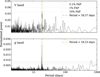 |
Fig. 8 Lomb-Scargle periodograms of the V band (top panel) and g′ band (bottom panel) photometry from ASAS-SN. The photometry are described in Section 3.3. The period of the highest peak is highlighted by a dash-dot green line, and it likely corresponds to the stellar rotation period. |
4 The joint transit and RV fit
We fit the photometry from TESS and a select light curve from ExTrA, plus the RVs from HARPS and NIRPS. As most of the other ground-based photometry from Section 2.2 were obtained during the timespan of the TESS observations, we elect to omit them from our joint fit model to avoid inflating the number of free parameters in return for little contribution towards improving the precision of the planet’s ephemeris. While we do not include most ground-based photometric data here, we ultimately use it to search for transit timing variations in Section 5.5. The exception to these omissions is the latest transit observation with ExTrA, which was taken on the night of 24 April, 2024, which occurred after the most recent TESS sector of data.
To perform the fit, we use the exoplanet package (Foreman-Mackey et al. 2020). exoplanet builds upon the light curve modelling package starry to compute transit models, the probabilistic programming library PyMC for MCMC sampling (Salvatier et al. 2016), and the fast Gaussian Process (GP) regression package celerite (Foreman-Mackey et al. 2017). We describe the joint fit model set-up below.
4.1 TESS photometry
We normalised the light curves for each TESS sector by its median out-of-transit flux level and concatenated all available sectors. This light curve showed a clear variability, as noted in Section 2.1, which we detrended using a GP whose kernel is a stochastically driven damped harmonic oscillator with a power spectral density of
 (1)
(1)
where Ω0 is the undamped angular frequency, Q is the quality factor, and S0 is proportional to the power at Ω = Ω0 Foreman-Mackey et al. (2017). We fit the maximum power,  , rather than S0 directly. Finally, we add a log jitter term, log(Jtess), as an additional error term to diagonal elements of the GP covariance matrix. Priors and posteriors on these parameters are reported in Table D.1.
We fit the planetary model components with a single Keplerian orbit model. The Keplerian model is parameterised by the planetary orbital period P, time of midtransit t0, orbital eccentricity e, and the argument of periastron ω. We discuss the eccentricity in Section 4.3. These parameters are used in light curve models created with starry, alongside the planetary radius Rp and stellar parameters. We use values from the TESS SPOC pipeline (Li et al. 2019) to place priors on P, t0, and Rp (see Table D.1). We use a limb-darkened transit model with the quadratic limb-darkening parameterisation from Kipping (2013). We use priors informed by the values on the stellar radius R* and the stellar mass M* derived in Section 3.
4.2 ExTrA photometry
The ExTrA light curves were extracted using the methodology established in Cointepas et al. (2021). These light curves exhibit systematic trends that we detrended using a GP with a Matern-3/2 kernel of the form
![Mathematical equation: \kappa(\tau) = \sigma^2 [(1+1/\epsilon)e^{-(1-\epsilon)\sqrt{3}\tau/\rho}(1-1/\epsilon)e^{-(1+\epsilon)\sqrt{3}\tau/\rho}],](/articles/aa/full_html/2026/05/aa58343-25/aa58343-25-eq19.png) (2)
(2)
where τ = |ti - tj| is the time lag between two observations taken at times ti and tj, and the hyperparameters are the amplitude scale σ and correlation timescale ρ. We adopt log-uniform priors on both hyperparameters (see Table D.1). We fit distinct limbdarkening coefficients from the TESS photometry as ExTrA’s wavelength coverage spans a unique wavelength range (i.e. 0.8-1.55 μm with ExTrA compared to 0.6-1.0 μm with TESS). Again, we use a quadratic limb-darkening parameterisation.
4.3 NIRPS and HARPS RVs
We try two different methods for fitting the NIRPS and HARPS RVs. The first incorporates no detrending and is solely a singleplanet Keplerian. The second incorporates an additional quasiperiodic GP kernel to detrend the NIRPS RVs, in order to remove the effect of the BERV crossing event described in Section 2.4. We do not include a GP on the HARPS data. We compare the evidence of the two models in Section 4.4.
We use DACE8 with a simple Keplerian model to estimate values for the systematic RV offsets and the semi-amplitude of the planetary signal in the RVs, K. The semi-amplitude of the planetary signal should be the same across the different wavelengths of NIRPS and HARPS, so we fit for one value between them. The RV offsets, however, are different, so we fit these separately (see Table D.1). We incorporate separate jitter terms for NIRPS and HARPS, which encapsulate any uncharacterised signal or noise that is perceived as white noise in the RV data. This could be, for example, instrumental effects, which will be different across the two instruments, and/or short-scale stellar activity. We use priors informed by the error on the NIRPS and HARPS data (see Table D.1), and the jitter is added in quadrature with the error on the RVs. For the first model, this is all that is incorporated.
For the second model, we are removing the effect of the BERV crossing window, which appears as a larger scatter in the RVs (Fig. 5) and also shows in the activity indicators (Fig. B.1). There are ∼20-day signals above the 10% FAP level in the NIRPS dLW, d Temp, and FWHM indicator. We detrend this signal using a quasi-periodic GP.
As in Osborn et al. (2021), we created our own quasi-periodic GP kernel using PyMC, as no such exact kernel is available in exoplanet. PyMC provides many simple covariance functions that can be combined. We used their Periodic kernel,
 (3)
(3)
and their ExpQuad (squared exponential) kernel,
 (4)
(4)
and we multiplied them together along with an additional hyperparameter to describe the amplitude of the GP, creating the quasi-periodic kernel9:
 (5)
(5)
The hyperparameters are η, the amplitude of the GP; θ, the recurrence timescale, which is the period of the signal; γ, the smoothing parameter; and λ, the timescale for signal growth and decay (e.g. Rasmussen & Williams 2006; Haywood et al. 2014; Grunblatt et al. 2015). This is commonly applied to stellar activity signals but is more broadly used to remove any quasiperiodic signal, so is applicable regardless of whether our signal is due to the BERV crossing or instead stellar activity (as noted in Section 3.3, there is a potential stellar rotation period of 18.5 d). We note that the Periodic term implemented by PyMC has a slightly different scaling than is commonly used (e.g. in Haywood et al. 2014), where 1 /2 is used as the exponent rather than two. We note that γ may be halved to recover the standard definition. We used a uniform prior on the recurrence timescale, as we sought to encompass the peaks present in the stellar activity indicator periodograms for NIRPS, the expected timescale of the BERV crossing event, and the potential stellar rotation period, and therefore we used a 10-40 day range. As λ is some multiple of the recurrence we cover a range from 1 to 10 times the bounds of our recurrence timescale prior. We bound the smoothing parameter between 0 and 1. The amplitude is given a wide prior.
As it is noted that warm Neptunes tend to present zero eccentricity (Correia et al. 2020), we run initial fits of both models (with and without the GP) with a uniform prior on eccentricity and argument of periastron. The posterior distributions in both cases indicate zero eccentricity, with the 95 per cent confidence interval of e < 0.094 for the model without the GP, and e < 0.099 with the GP. We therefore elected to fix e to zero in the final model presented here. This is further justified by the expectation that the planet should be tidally circularised given its short orbital period of ∼3.6 days. We also note that there is no change in fit values of any parameters within error whether eccentricity is fixed to zero or not.
4.4 Sampling the joint model posterior
We fit two models as described in Section 4.3: model 1 incorporates no detrending of the RVs while model 2 incorporates a quasi-periodic GP to detrend the NIRPS RVs. We follow the same procedure to estimate each model’s joint posterior probability density function as outlined below.
We first use exoplanet to maximise the log-posterior probability of the model. We use the best-fit values from this optimisation as the starting point of the PyMC sampler. PyMC draws samples from the posterior using the No-U-Turn Sampler, a variant of Hamiltonian Monte Carlo. We examine chains from earlier test runs of the model to inform our choice of 4 chains of 60 000 steps, with an additional 1000 steps that are discarded as burn-in. We calculate the rank-normalised split-R̂ statistic (Vehtari et al. 2021) for each parameter to test for non-convergence. For both models, R ≈ 1.0 for all parameters, implying both models have converged.
To identify which model is statistically favoured, we calculate and compare the Bayesian evidences Z for each model using the Perrakis estimator (Perrakis et al. 2014). We calculate an evidence ratio (i.e. Zmodel2/Zmodel1) of 5.88. This ratio (or Bayes factor) is not large enough to conclude that model 2 is statistically favoured by our data (Nelson et al. 2020), but because we are physically motivated to remove the BERV crossing signal in the NIRPS RVs, we choose to go with model 2. The results from model 2 are thus what we report as our final model parameters in Table 3 using the median values from the marginalised posteriors and the 16th and 84th percentiles as the approximate 1σ errors. We also highlight that the RV semi-amplitudes recovered in both models are consistent, where  m s−1 and
  ms−1, so the choice of model should not affect the conclusions we draw about this planet.
Transit, orbital, and physical parameters of the planet TOI-672 b.
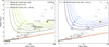 |
Fig. 9 Mass-radius diagrams showing TOI-672 b (yellow star) against the well-characterised planet population (light grey dots) from the PlanetS catalogue, available at https://dace.unige.ch/exoplanets. It contains planets with precisions on planet mass and radius of <25 and 8%, respectively (Otegi et al. 2020; Parc et al. 2024). Planets around M dwarf hosts (i.e. Teff < 3900 K and M*, R* < 0.6 M⊙, R⊙) are highlighted as dark grey dots. Solar System planets are shown for comparison (outlined circles, labelled). Both panels show mass-radius relations from Skinner et al. (2026) for Earth-like rocky (32.5% core + 67.5% mantle) compositions (dark brown) and pure rock (100% mantle) compositions (light brown). Both panels also show model mass-radius relations from Skinner et al. (2026) (solid lines), as described in Section 5.2 for an equilibrium temperature of 700 K, with annotated percentages reporting the hydrogen mass fraction of each curve. The mass-radius relations in the left panel correspond to an Earth-like core composition (i.e. 32.5% iron + 67.5% mantle), while the right panel assumes a 50% water plus 50% Earth-like core composition. |
5 Results and discussion
5.1 Planetary parameters
We measure the mass and radius of TOI-672 b to be  M⊕ and
  R⊕, respectively. TOI-672b is a massive superNeptune orbiting an M0V star every 3.63 days. Our measured radius and period agree with the previously measured values reported in the TOI release and validation paper (Mistry et al. 2023). However, the planet is much more massive than predicted by the Chen & Kipping (2017) mass-radius relations presented in Mistry et al. (2023) (i.e. 24.2 ± 10.7 M⊕). Nonetheless, the planet’s low density of
  g cm−3 suggests that it has a significant H2-He envelope, which we explore in Section 5.2. We compare the mass and radius of TOI-672b to the known, well-characterised planet population in Fig. 9. There are no planets around M dwarfs with similar masses and radii; TOI-1728b is the closest in radius at
  R⊕ with a similar period of 3.49 d, but only half the mass,
  M⊕ (Kanodia et al. 2020); it has a low precision on its mass measurement and so does not feature in Fig. 9. It does, however, probably lie on a similar composition track to TOI-672 b (see Section 5.2), as does TOI-674 (P = 1.98 d, Murgas et al. 2021) and GJ 3470b (P = 3.34d, Awiphan et al. 2016). Kepler-101 b has very similar properties (3.63 d;
  M⊕;
M⊕;  R⊕), but it is orbiting a G3 star (Bonomo et al. 2014) and so has a higher equilibrium temperature.
TOI-672 b is moderately irradiated by its host star with an instellation of 39.8× Earth’s instellation and an equilibrium temperature of 699.5 K (assuming an albedo of zero and full heat redistribution). It has a Transmission Spectroscopy Metric (TSM) and Emission Spectroscopy Metric (ESM) of 69−10 and 26 ± 3, respectively (Kempton et al. 2018). With its Neptunian size and short orbital period, TOI-672 b falls within the Neptune desert as defined by Mazeh et al. (2016). That study, however, focuses on FGK planet hosts, and we revisit the desert boundaries for FGK versus M dwarf hosts in Section 6.
5.2 Planetary composition
We added TOI-672 b to the mass-radius diagram in Fig. 9. We compared the known exoplanet population to a suite of compositional curves, including novel mass-radius relations for irradiated, H2-He-dominated planets (Skinner et al. 2026). We used these novel compositional mass-radius relations because the somewhat unique mass and radius of TOI-672 b place it in a region of the parameter space for which we are unaware of any existing mass-radius relations in the recent literature.
Here we provide a brief summary of our interior structure models, which are detailed by Skinner et al. (2026). Planets are assumed to be differentiated bodies in hydrostatic equilibrium with convective interiors and atmospheres following the radiative transfer-informed temperature profile of Parmentier & Guillot (2014); Parmentier et al. (2015). Planets are composed of an Fe-rich core with mixed-in volatile O and S, a mantle with full mineralogy composed of FeO, SiO2, MgO, and combinations thereof (e.g. MgSiO3), a multi-phase layer of pure water that uses the AQUA models to calculate the non-isothermal H2O equation of state (Haldemann et al. 2020), and a non-ideal H2-He envelope with an opacity arising from a 50× solar metallicity equilibrium mixture of metals. This metallicity is in line with the metallic-ity expected for a planet of this mass following mass-metallicity relationships and similar to Uranus and Neptunes’ atmospheric metallicities (Swain et al. 2024). As this model is for a static interior, it cannot directly capture the crucial physics of envelope contraction. This is accounted for by including internal luminosity in the outer temperature boundary condition following the models of Mordasini (2020). Without a constrained stellar age, we assume a planetary age of 4.5 Gyr, analogous to the Solar System and the near average of the potential system ages considered in Section 5.3. Given an input planetary mass, instellation, age, and core, mantle, water, and envelope mass fractions, we solve the standard differential equations of planetary structure to calculate the planet’s transit radius by integrating the atmospheric optical depth along a grazing chord as observed through a transit geometry (Guillot 2010). Since the refractory abundance ratios Fe/Mg and Mg/Si of TOI-672 are consistent with solar (c.f. Table 2), we consider two fiducial core compositions in the mass-radius relations depicted in Fig. 9. The first is an Earth-like composition (i.e. 32.5% core + 67.5% mantle, mantle molar MgZSi=1.205 and Fe/Mg=0.123; left panel) and the other a water-rich core (i.e. 50% water + 50% Earth-like; right panel), as is expected for a water-rich core formed from solar metallicity material beyond the snowline (Lodders 2003).
Our models imply that TOI-672 b is consistent with having a H2-He envelope mass fraction of 20-30%, depending on the assumed water mass fraction of the core. In contrast, the massradius curves of Fortney et al. (2007), which are computed using an evolutionary planetary interior model rather than a static one as considered here, imply a lower H2-He envelope mass fraction of ∼11% (see their Fig. 7). Fortney et al. (2007) do not account for high-pressure phase transitions, resulting in a systematic underprediction of planetary densities leading to lower inferred H2-He abundances. We note that the stellar refractory abundances are insufficient to constrain the core compositions because TOI-672 b may have a core that is volatile-rich, which is largely set by its unknown formation location and evolutionary history. Additionally, the unconstrained age of TOI-672 means that it is impossible to determine how much envelope contraction has occurred, introducing a degeneracy between the inferred planetary radius and its age.
5.3 Atmospheric evolution
We explored the scenario in which TOI-672 b migrated early on within the protoplanetary disk and started evolving on its present-day orbit, performing atmospheric evolutionary simulations of TOI-672 b with the JADE code (Attia et al. 2021, 2025)10 according to the procedure detailed in Bourrier et al. (2025). As the age of TOI-672 remains largely unconstrained, we performed simulations for a range of field ages that includes 1, 5, and 10 Gyr.
First, rotating stellar models representative of TOI-672 were computed with the Geneva stellar evolution code (GENEC, Eggenberger et al. 2008) using stellar radius and effective temperature constraints given in Table 2. These models account for the internal transport of angular momentum by hydrodynamic and magnetic instabilities (see e.g. Eggenberger et al. 2022). Based on the structural and rotational evolution of these models, the evolution of the high energy fluxes emitted by the host star is then deduced (see Pezzotti et al. 2021). The initial velocity of the star being unknown, we consider the case of a moderate rotator with an initial rotation rate of 5 Ω⊙ (see Eggenberger et al. 2019). This rotational history then results in a given evolution of the X-ray luminosity of the host star and to a corresponding extreme ultraviolet luminosity computed with the relation between the X-ray and extreme ultraviolet luminosity provided by Sanz-Forcada et al. (2011) (see e.g. Pezzotti et al. 2021). The stellar luminosity was set to the GENEC evolutionary curve at the three assumed ages.
We then use the JADE internal structure solution for TOI-672b, which we condition on our findings from Section 5.2. Namely, the mass and orbital properties of the planet were set to their nominal present-day values and the envelope mass fraction was fixed to 0.2, which is consistent with our findings in Section 5.2. Uniform priors (U(0,1)) were set on the atmosphere (fEnv/Pl) and mantle (fMa/Pl) mass fractions relative to the total planet mass, and a narrower prior (U(0,0.1)) on the trace atmospheric metallicity, although this value is not constrained by our data. The retrieval is constrained by the measured planet radius. We find that the derived fEnv/Pl increases with the assumed system age, from  % for 1 Gyr to
  % for 10Gyr, corresponding to absolute median solid and envelope masses of 43.2 and 7.7M⊕ for 1 Gyr and 41.8 and 9.1 M⊕ for 10Gyr. This is likely because the atmosphere cools and shrinks as stellar irradiation decreases over time, so that a larger atmospheric mass fraction and lower bulk planetary density are required to yield the same radius at a more advanced age.
We then simulated the atmospheric evolution of TOI-672 b with JADE over a grid of initial planet mass, running three sets of simulations from the expected dissipation of the disk (10 Myr) up to the assumed present-day ages. System properties were fixed to their present-day values from Table 3, and to the results of the internal structure retrieval for each age. The stellar luminosity curve was set to the model computed with GENEC. The evolutionary retrieval was performed as described in Bourrier et al. (2025), constrained by the present-day planet radius and assumed system age. Results are shown in Fig. 10. Most atmospheric erosion would have occurred within the first 300Myr, when the star was most active, although the planet may only have lost about 20% of its primordial envelope mass during this phase. Indeed, atmospheric escape is made inefficient by the strong gravity of TOI-672 b. Even for an assumed system age of 10 Gyr, the planet would subsequently have lost <10% of its remaining envelope mass. Initial masses derived for TOI-672b are consistent within 1σ across the three assumed ages, ranging from  M⊕ to
M⊕ to  M⊕. The corresponding initial planet radius would be on the order of 6.1-6.5R⊕, so that the nature of TOI-672 b would not have changed substantially across its evolution.
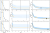 |
Fig. 10 JADE exploration of TOI-672 b atmospheric evolution, assuming ages of 1, 5, and 10 Gyr (top, middle, and bottom rows, respectively). Left column : probability density function of the initial planet mass. The median is highlighted as an orange line, and the 1σ HDI interval is shown as dashed blue lines. Middle column : temporal evolution of the planet envelope mass in the best-fit simulation (orange curve) and a set of simulations from within the HDI interval (blue curves). The vertical black line with a grey shaded band marks the assumed age and uncertainties. Right column : same as the middle panel, but for the planet radius. The black point indicates the measured value. |
5.4 RV sensitivity to additional planets
Multi-planet systems are common around M dwarfs (Bonfils et al. 2013; Tuomi et al. 2014; Dressing & Charbonneau 2015; Gaidos et al. 2016; Cloutier et al. 2021a; Mignon et al. 2025). In particular, Dressing & Charbonneau (2015) and Gaidos et al. (2016) found that early M dwarfs host an average of 2.5 small, short period planets per star while  % of mid-to-late M dwarfs host multiple small planets (Cloutier et al. 2021a). It is therefore reasonable to expect additional planets around TOI-672 that have insofar remained undetected by TESS and our RV analysis due to either a long orbital period, low inclination, or small size and/or mass. Here we quantify the sensitivity of our RV dataset to additional planets in the TOI-672 system.
We calculate the detection sensitivity of our RV time series as a function of orbital period and planet mass via a set of injection-recovery tests. Our procedure follows the methods of Cloutier et al. (2021b) and Cherubim et al. (2023). We inject synthetic Keplerian signals into the residuals of our RV time series. We produce 105 realisations of Keplerian signals produced by a single planet with planet masses and orbital periods sampled uniformly in log space from 1 to 70 M⊕ and 1-1000 d, respectively. Orbital phases are sampled uniformly from 0 to 2π; we sample orbital inclinations as a Gaussian distribution centred on the median value of inclination from our joint fit (i.e. 88.0°) with a dispersion in mutual inclinations of 2° following Ballard & Johnson (2016). We note that this results in mostly coplanar planets being injected. We sample the stellar mass from its posterior and calculate the RV semi-amplitude due to the injected planet assuming a circular orbit. By injecting the Keplerian signal into the RV residuals, we preserve any residual noise that was not perfectly detrended and we maintain the individual measurement uncertainties and time stamps.
We then attempt to recover the injected planets as signals that satisfy two criteria. First, a recovered signal must appear in the Generalised Lomb-Scargle (GLS) periodogram (Zechmeister & Kürster 2009) with a FAP ≤ 1% and whose period is within 5 % of the injected period. The GLS periodogram is created for each realisation and the FAP is calculated analytically (Zechmeister & Kürster 2009). Secondly, the Keplerian model must be statistically favoured over a flat line. We base the model comparison on the difference in Bayesian Information Criterion (BIC) between the two models; BIC = 2ln L + ν ln N, where L is the Gaussian likelihood of the RV data given the assumed model, ν is the number of model parameters (one or six for the null or Keplerian models, respectively), and N is the number of RV measurements. Our second detection criterion is therefore ∆BIC = BIC Keplerian — BIC null ≥ 10 (Cloutier et al. 2021a; Cherubim et al. 2023). We define the sensitivity of our RV data as the ratio of the number of recovered planets to the number of injected planets per bin, which is shown in Fig. 11.
Fig. 11 highlights the different levels of sensitivity between our HARPS and NIRPS data. We note that there are less HARPS data than NIRPS, and only one HARPS point after the time span in which the star was unobservable (Fig. 5). We also note that the apparent improved sensitivity at approximately 9 and 200 days is likely due to aliasing in the periodogram of the RVs, i.e. it is artificial and a region of high false detection probability rather than enhanced sensitivity.
Considering orbital periods out to 200 days, with our NIRPS data we expect to detect approximately 40% of signals with a semi-amplitude of 10ms−1. With the HARPS data, there is no sensitivity to signals of this semi-amplitude; we only start to become sensitive to semi-amplitudes above 20 ms−1. Combining the two datasets slightly improves the sensitivity. It is also worth noting here that, despite the NIRPS sensitivity being better, using HARPS+NIRPS gives double the amount of RV measurements for the same time investment, as they operate simultaneously.
We can reliably detect planets the mass of TOI-672 b out to around 100 d orbital periods. With the RV data in hand, we are unable to recover small terrestrial planets with Mp ≤ 5 M⊕, even at very short orbital periods of 1 day. Our data are also insufficient to probe super-Earth mass planets (Mp ≲ 20 M⊕) within the habitable zone bounded by the moist greenhouse inner edge and the maximum greenhouse outer edge (shaded in Fig. 11, Kopparapu et al. 2013).
5.5 Searching for transit timing variations
Here we search for transit timing variations (TTVs) by fitting the individual transits from TESS, ExTrA, and the other groundbased facilities. The baseline of these data is 518 days. We excluded several transits within these datasets due to excessive noise or a lack of clear ingress or egress. These excluded observations include two nights of ExTrA observations from all telescopes on the nights of 16 February 2023 and 8 April 2023, and both Evans 0.36 m telescope observations. In total, we use 51 transits, listed in Table A.1. We follow the method outlined in Sections 4.1 and 4.2 to fit transit models to each individual transit event. We adopt Gaussian priors on the stellar radius and mass, planetary period, and radius based on the results of our full joint fit model (Table D.1). The mid-transit time is left free to vary with a uniform prior whose width spans the full duration of the transit observation. The TESS light curves are detrended with the SHO GP as described in Section 4.1; the ExTrA light curves are detrended with the Matern 3/2 GP as described in Section 4.2; the remaining ground-based light curves require no detrending further to what was presented in Mistry et al. (2023).
The resultant mid-transit times for each transit are provided in Table A.1 and shown in Fig. 12.
We find no evidence of TTVs in the transits of TOI-672 b. The root mean square (rms) deviation across all transits is 1.7 minutes. The TESS transits show the smallest deviation with a maximum of 2 minutes and rms of 1.3 minutes. The typical uncertainty on t0 is 1.4 minutes for TESS, 2.3 minutes for ExTrA, and 1.6 minutes for the other facilities. The χ2 statistic comparing the individual mid-transit times to the linear ephemeris is 0.76, indicating that the transit times are consistent with no detectable TTVs, and that the transit time uncertainties might be slightly overestimated. We perform least-squares minimisations to fit a straight-line model and then a quadratic model to the transit times, and compare these models to the linear ephemeris model. Neither of these more complex models are preferred as their ∆ BIC values are >3 and 5, respectively. We also examine a Lomb-Scargle periodogram of the mid-transit times and uncover no significant periodicities.
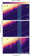 |
Fig. 11 Sensitivity of the RV data, specifically the NIRPS data (top panel), HARPS data (middle panel), and combined NIRPS plus HARPS data (bottom panel), to additional planets orbiting TOI-672 as a function of planet mass and orbital period (using 50 × 50 bins in this parameter space). The calculation is described in Section 5.4. The sensitivity is shaded as in the colour bar, from 0 (dark purple) to 1 (light yellow). The 90 and 10% sensitivity limits are denoted by the dark purple and medium purple solid lines, respectively, and labelled in the top panel. The RV semi-amplitudes of 20, 10, 5, and 1 m s−1 are denoted by the red, orange, yellow, and white dashed lines, respectively, and labelled in the top panel. TOI-672 b is shown by the star marker (where error bars are too small to be seen). The habitable zone defined by Kopparapu et al. (2013), specifically the moist greenhouse inner edge and the maximum greenhouse outer edge calculated for the specific host star TOI-672, is shaded with a turquoise colour. |
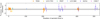 |
Fig. 12 Searching for TTVs in the transits of TOI-672b. Mid-transit times from fits to each individual transit (described in Section 5.5) are compared to the linear ephemeris from the joint fit model (i.e. the dark grey line at y = 0 in this plot, where the 1, 2 and 3 standard deviations from the value are shaded). The TESS transits are shown as orange circles; the LCO CTIO transit is the yellow triangle; the PEST transit is the green pentagon; the LCO SSO transit is the blue upside down triangle; the ExTrA transits are purple squares; and the Deep Sky Chile CDK17 transit is the orchid coloured diamond. |
6 M dwarf Neptunian desert
We place TOI-672 b in the period-radius diagram in Fig. 1 and overplot the Neptunian desert boundaries from Mazeh et al. (2016) and Castro-González et al. (2024) (hereafter CG24). TOI-672 b appears to lie in the newly coined Neptunian ridge (CG24). However, planets orbiting M dwarfs are highly under-represented in these boundary studies due to observational biases. The desert boundaries may not uniformly apply to all systems due to differences in the environments of planets around M dwarfs compared to earlier type stars. Indeed, Hallatt & Lee (2022) predict that the boundaries of Neptunian desert in radius-period space should be altered around different types of host stars due to the planets’ differing radiation environments and evolutionary histories. Here we explore for the first time the consistency of the Neptune desert boundaries between M versus FGK dwarfs in periodradius space, and also extend our analysis to instellation-radius space.
We build off the methodology presented in CG24. However, the number of M dwarf systems in the Kepler DR25 catalogue is limited, which inhibits a meaningful statistical comparison between the M and FGK system properties. We instead use the catalogue of Berger et al. (2023) (hereafter B23), which presents homogeneous, precise stellar parameters for Kepler, K2 and TESS host stars, and consequent planetary parameters based on Gaia DR3 astrometry. Homogeneous stellar properties are important as the significant systematics between the different methodologies for determining these propagate into the determination of the physical parameters of the planets like radii and masses. Using a consistent method for determining parameters means comparing like-for-like.
We applied several cuts to this catalogue to produce our final sample. We begin by restricting our sample to planets discovered by Kepler and TESS. We exclude K2 discoveries as the recovery fraction of planets from the K2 light curves is significantly lower than Kepler (Zink et al. 2021). We only include “confirmed” and ‘known’ planets (dispositions of ‘CP’ and ‘KP’, respectively). We excluded planet candidates, as the high incidence of false positives within the Neptunian desert (see e.g. Sanchis-Ojeda et al. 2014; Lillo-Box et al. 2024; Doyle et al. 2025) would contaminate our sample if included. We also identified and removed post-main-sequence stars that do not satisfy the temperature-dependent stellar radius filter given by Eq. (1) in Fulton et al. (2017):
 (6)
(6)
where the stellar effective temperature Teff is given in kelvin. We also eliminate stars earlier than F0V and later than M9.5V by restricting to stars with 2300 < Teff (K)< 7300 K.
The B23 catalogue uses Rp/R* in combination with their computed stellar radii to recalculate the planet radii. For the Kepler planets, Rp/R* comes from the Cumulative KOI table at the NASA Exoplanet Archive, which provides accurate planetary parameters. As such, we then use the planet radius values Rp from B23. By contrast, the parameters for the TESS planets come from the TOI catalogue (Guerrero et al. 2021). These are the values provided when a TESS planet was released as a candidate, and they have not been updated to match parameters from later refereed publications on the systems. The latter are generally considered more reliable but are available for known and confirmed planets only. This is no issue for this study, as we restricted our sample to only known and confirmed planets. Therefore, we performed a cross-match with the NASA Exoplanet Archive11 to obtain published Rp/R* values for our TESS planets, and then use R* from B23 to recalculate Rp. The B23 catalogue also provides stellar luminosity values, which we can combine with their semi-major axis values to compute instellations, S, for all of our planets.
We account for the biases in our sample from geometric transit probability and detection sensitivity using the method of CG24. In short, we use an inverse detection efficiency method where the probability of each planet in our sample being detected around its host star is calculated. Each planet’s detection probability is used to weight the planet in our sample according to
 (7)
(7)
Here, Ptransit is the geometric transit probability:
 (8)
(8)
where a is the planet’s semi-major axis taken from B23. Pdetection is the signal recoverability, i.e. the probability of detecting a planet given the S/N of its combined transit signal. For the Kepler pipeline, signal recoverability is well described by a gamma cumulative distribution of the form
 (9)
(9)
where x is the transit S/N and the best fit coefficients for the DR25 catalogue are a = 33.54, b = 0.2478, and c = 0.9731 (Christiansen et al. 2020), which we adopt here. Unfortunately, no similar calculation is publicly available yet for the TESS Transit Search Pipeline, and performing this analysis is beyond the scope of this work. As an ad hoc solution, we follow Rodel et al. (2024) and apply the Kepler distribution in Eq. (9) to our TESS targets. Of course, there are many differences between the TESS and Kepler missions (e.g. aperture size, precision, observation baseline, brightness of target stars), and their respective pipelines (with our confirmed planets from TESS being discovered by multiple pipelines). This work is therefore more of an illustrative first look at these Neptunian desert boundaries, and can be improved upon in the future.
The S/N of the transit signals in the Kepler pipeline can be calculated as
 (10)
(10)
where δ is the transit depth, σCDPP is the rms combined differential photometric precision (CDPP) computed at the transit duration (Christiansen et al. 2012), and N is the number of transits observed. For the Kepler planets in our sample, we obtain N and σCDPP values for each target from Kepler DR25, as well as the impact parameter. We use the impact parameter alongside the stellar radii, planetary radii, and orbital periods from B23 to reconstruct the transit duration. We then use the value of the σCDPP calculated for the closest matching transit duration (the available transit durations range from 1.5 to 15 hours) for each target in our sample.
The S/N of transit signals in the TESS pipeline can also be calculated using Eq. (10), but this only holds for one sector of observations because the CDPP values for the same star can vary across sectors (Twicken et al. 2025). The S/N for multiple sectors is calculated as
 (11)
(11)
such that Ni transits are observed in sector i (Twicken et al. 2025)12. Here, we use transit duration and depth from the TOI catalogue and again use the value of the σCDPP calculated for the closest matching transit duration (in this case, the available transit durations range from 0.5 to 15 hours) for each target in our sample. Finally, we remove any planets with S/N < 7.1, which is the Kepler pipeline detection threshold.
To split the sample into FGK planet hosts versus M dwarf planet hosts, we define M dwarfs as Teff < 3900 K. In summary, our sample is drawn from Kepler and TESS known and confirmed planets, and contains 146 planets around 105 M dwarf hosts, and 2637 planets around 1994 FGK hosts, whose parameters are provided in Table E.1 and displayed in Fig E.1.
Unfortunately, with so few M dwarf planets, the Gaussian kernel density estimate (KDE) method of CG24 results in uninformative desert boundaries. We therefore devised an alternative approach to calculating the desert boundaries, which we apply to the M dwarf and FGK samples separately, as well as to the combined sample for comparison. We do this in both period-radius space, as is used in CG24, and also instellation-radius space.
We split our samples into eight equal size bins in {log Rp, log P} (or {log Rp, log Sp}) space. Following CG24, we restrict the parameter space the bins cover to 1 < Rp < 25 R⊕ and P < 30 days, in order to avoid areas of parameter space that have uncorrectable incompleteness, i.e. where very few or no planets have been detected (we keep this period cut for the sample in instellation space also). The number of bins is restricted by our M dwarf sample, which has 18× fewer planets compared to those around FGK stars from Kepler and TESS. To account for uncertainties in the radii and period (or instellation) of each planet, we sample 105 realisations from normal distributions of each planet’s radius and period (or instellation) given its reported 1σ errors. For each realisation, we calculated the 2.3, 16, 84, and 97.7 percentiles of the orbital periods (or instellations) in each radius bin. In these calculations, each planet is weighted by w given in Eq. (7). We then take the mean and standard deviation of these percentiles over the 105 realisations as our final period (or instellation) distributions, which are displayed in Fig. 13 for period-radius space, and in Fig. 14 for instellation-radius space. Finally, we adopt the 2.3 percentile values as the edges of the Neptunian desert, which are shown in Fig. 15 for period-radius space, and in Fig. 16 for instellation-radius space.
We first looked at our boundaries in period-radius space. We produced a desert shape similar to that from Castro-González et al. 2024, where the triangular tip, as in Mazeh et al. (2016), is truncated. It is worth noting here that there are very few giant planets in our M dwarf sample, making the errors on the upper boundary, i.e. bins 7 and 8, very large. It could be the case that the upper boundary does not present in the same way for M dwarf planets, but this might change if we discover more planets in this regime.
As introduced in Section 1, Hallatt & Lee (2022) predict that the opening of the Neptunian desert, where the upper and lower boundaries intersect, should shift to shorter orbital periods around M dwarfs. This begins at ∼0.7 days around 0.5 M⊙ stars and ∼1.5 days around 0.8 M⊙ stars, compared to ∼3 days around 1 M⊙ stars. By taking the weighted average of the 2.3 percentiles for bins 3-5 (labelled in Fig. 13), we can estimate the period at which the desert opens. The average stellar mass of our FGK sample is 0.99 ± 0.2 M⊙ and we find the opening at 3.3 ± 1.4 days, matching the prediction. The average stellar mass of our M dwarf sample is 0.43 ± 0.13 M⊙, and while the opening shifts to a slightly lower period as predicted, we find the opening is located at 2.2 ± 1.0 days. This is within ∼1 σ of the period for the FGK hosts and in slight tension with the predicted 0.7 days (Hallatt & Lee 2022).
The prediction of Hallatt & Lee (2022) is predicated on atmospheric mass loss processes as the dominant mechanism in opening the desert. The discrepancy between our observation and the theoretical prediction might mean that they are not. CG24 remark that the period range of the Neptunian ridge is similar to the hot Jupiter pileup and note that a large number of Jupiter and Neptune-sized planets with eccentric, misaligned orbits exists in these over-dense regions. Thus, they posit that high-eccentricity migration may be the main process bringing planets into the ridge. The mechanisms sculpting the desert and the ridge should be explored further once a larger sample of M dwarf planets will make comparisons of planets across stellar types more robust. This may be accomplished through looking at atmospheric escape efficiencies and spin-orbit angles of planets in and around the desert.
Next we considered the desert boundaries in bolometric instellation-radius space. Unlike the boundaries in period-radius space, we find that the desert boundaries around FGK hosts versus M dwarf hosts are differ significantly with the latter boundaries occurring at much lower bolometric instellations. Repeating the same boundary calculation as in period-radius space, we estimate the instellation at which the desert opens to be 830.7 ± 0.1 S⊕ around FGK stars compared to 57.8 ± 0.2 S⊙ around M dwarfs. In both parameter spaces, TOI-672b is located just outside the desert.
Photoevaporation caused by X-ray and Extreme Ultra-Violet (together, XUV) radiation from host stars is believed to be a main driver of the Neptunian desert’s lower boundary (Owen & Lai 2018). However, the XUV luminosity histories of the host stars in our sample are unknown, which necessitated our consideration of the desert as a function of bolometric instellation. What is known is that the ratio of XUV luminosity to bolometric luminosity differs across stellar types, as does the evolutionary timescale for the saturated phase of high XUV emission, prior to the emission falling off as stars age and spin-down (Jackson et al. 2012; Shkolnik & Barman 2014; Pass et al. 2025). In general, later type stars exhibit longer saturation timescales and higher XUV:bolometric luminosity ratios. As such, we expect that per bolometric instellation, planets orbiting field-age M dwarfs will experience higher levels of lifetime XUV irradiation compared to around FGK stars (McDonald et al. 2019). While present day bolometric instellation is not the main driver of the location of the desert, the location of the M dwarf boundary at lower bolometric instellations than around FGK stars in Figure 16 is consistent with predictions from XUV-driven photoevaporation. However, it is important to note that the boundary for M dwarf hosts in instellation space could not overlap the boundary for FGKs. At an instellation of ∼800 S⊕ (the position of the boundary for FGKs), a Neptune around an average M dwarf in our sample would experience tidal disruption due to its proximity to the Roche radius of its star. Nevertheless, the current placement of the boundary at ∼60 S⊕ for M dwarfs is far outside the Roche radius, so we do not expect its placement to be sculpted primarily by tidal disruption.
Future work should focus on calculating the lifetime XUV irradiation for all planets in our sample (noting that McDonald et al. (2019) only do this for lifetime X-ray irradiation), and recalculating the desert boundaries. If XUV photoevaporation is the main driver of the desert boundaries, then the empirical boundaries in lifetime integrated XUV irradiation-radius space should be consistent across different spectral types.
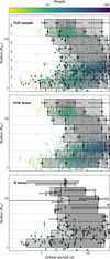 |
Fig. 13 Study of the Neptunian desert boundaries for FGK planet hosts versus M dwarf hosts in period-radius space, as described in Section 6. Our planet sample (Table E.1; Fig. E.1) is shown as coloured dots, according to the weighting of each planet. In the top panel, our full planet sample is shown (where M dwarf hosts are highlighted with black outlines). The middle panel shows planets around FGK hosts only, and the bottom panel shows planets around M dwarf hosts. The boundaries of the bins in radius space are depicted with dashed lines and the bins are numbered 1-8 in the top panel. The period percentile values calculated for each bin and their errors are shown. The 2.3-97.7 percentiles are shaded in light grey, while the 16-84 percentiles are shaded in dark grey. |
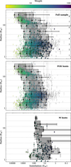 |
Fig. 14 Study of the Neptunian desert boundaries for FGK planet hosts versus M dwarf hosts in instellation-radius space, as described in Section 6. The details are the same as in Fig. 13. |
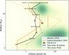 |
Fig. 15 Comparison of the Neptunian desert boundaries in periodradius space as derived by Mazeh et al. (2016) (yellow dotted lines), Castro-González et al. (2024) (orange dashed lines), and this work, where we calculated the desert boundaries for FGK planet hosts (grey solid line) and M dwarf hosts (black solid line) separately. The background is shaded according to the known planet population from the NASA exoplanet archive, as in Fig. 1. |
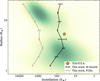 |
Fig. 16 Comparison of the Neptunian desert boundaries in instellation-radius space as derived in this work, where we calculated the desert boundaries for FGK planet hosts (grey solid line) and M dwarf hosts (black solid line) separately. The background is shaded according to the known planet population from the NASA exoplanet archive, as in Fig. 1. |
7 Conclusions
In this study we confirmed and characterised the previously validated planet TOI-672b. We used photometry from four TESS sectors and a single transit observation from ExTrA, and we modelled these data jointly with RV data taken with the NIRPS and HARPS spectrographs.
We used empirical M dwarf relations to measure the mass and radius of the M0V star TOI-672 as well as the spectra from NIRPS to obtain its effective temperature and individual elemental abundances, from which we derived its overall metallicity [M/H] and α-enhancement [α/Fe]. We estimate the stellar rotation period to be 18.5 days based on ASAS-SN photometry. This value is within the range of predicted periods from the log R′HK.
We showed that TOI-672 b is a massive super-Neptune with a period of 3.63 days, a radius of  R⊕, and a mass of
  M⊕. We presented novel mass-radius relations for irradiated H2 -He-dominated planets and determined that TOI-672 b has a H2-He envelope mass fraction of 20 - 30% (depending on the assumed core composition). We performed atmospheric evolution simulations, assuming early migration and evolution at the present-day orbit of TOI-672 b. We find that the nature of TOI-672 b would not have changed substantially over its lifetime, as atmospheric escape is made inefficient by its strong gravity.
The period and radius of TOI-672 b place it within the Neptunian desert or ridge. However, existing desert boundaries have been calculated from planets predominantly orbiting FGK stars. We have performed the first study that directly compares the Neptunian desert boundaries in both period-radius space and instellation-radius space for planets hosted by FGK stars versus M dwarf stars. We devised a novel method for determining the desert boundary and reproduced a truncation of the righthand-side of the desert in period-radius space (the ridge, as in CG24), and we find this opening of the desert to be at comparable periods of 2.2 ± 1.0 days and 3.3 ± 1.4 days for M dwarf hosts and FGK hosts, respectively. This shift is small compared to theoretical predictions based on atmospheric escape processes (Hallatt & Lee 2022). We find that in instellation-radius space, the boundary changes significantly between M-dwarf and FGK hosts, shifting to lower instellations for the former. We encourage further study of the mechanisms sculpting the desert and ridge in order to better determine the predominant processes and whether the desert changes across stellar types.
Lastly, we explored the possibility of additional planets in the TOI-672 system. The system was selected as a favourable target for the NIRPS GTO ‘Deep Search’ sub-program due to its potential for having additional planets not seen in transit. We used the photometry from TESS, ExTrA, and other ground-based facilities to search for TTVs, for which we find no evidence. We quantified the sensitivity of our RV time series and found that from 1-200 d, we would expect to recover signals down to approximately 10ms−1 with the combined NIRPS and HARPS data, and thus we were unable to recover any small terrestrial planets below 5 M⊕ that could be present.
Data availability
Tables C.1 and E.1 are available at the CDS via https://cdsarc.cds.unistra.fr/viz-bin/cat/J/A+A/709/A23. Tables B.1, B.2, and B.3 are available on ExoFOP-TESS at https://exofop.ipac.caltech.edu/tess/target.php?id=151825527. The code underlying the joint fit is available on reasonable request to the corresponding author.
Acknowledgements
We first thank the anonymous referee for their comments which improved the quality of this manuscript. We would like to thank George W. King for helpful discussion regarding XUV-driven photoevaporation. A.O. acknowledges this research was part funded by the UKRI (Grants ST/X001121/1, EP/X027562/1). This project has received funding from the European Research Council (ERC) under the European Union’s Horizon 2020 research and innovation programme (project SPICE DUNE, grant agreement No 947634). This material reflects only the authors’ views and the Commission is not liable for any use that may be made of the information contained therein. This work has been carried out within the framework of the NCCR PlanetS supported by the Swiss National Science Foundation under grants 51NF40_182901 and 51NF40_205606. N.J.C., É.A., C.C., A.L., F.Ba., B.B., R.D., L.Ma., R.A. & J.P.W. acknowledge the financial support of the FRQ-NT through the Centre de recherche en astrophysique du Québec as well as the support from the Trottier Family Foundation and the Trottier Institute for Research on Exoplanets. N.N., J.I.G.H., R.R., A.S.M. & A.K.S. acknowledge financial support from the Spanish Ministry of Science, Innovation and Universities (MICIU) projects PID2020-117493GB-I00 and PID2023-149982NB-I00. N.N. acknowledges financial support by Light Bridges S.L, Las Palmas de Gran Canaria. N.N. acknowledges funding from Light Bridges for the Doctoral Thesis “Habitable Earth-like planets with ESPRESSO and NIRPS”, in cooperation with the Instituto de Astrofísica de Canarias, and the use of Indefeasible Computer Rights (ICR) being commissioned at the ASTRO POC project in the Island of Tenerife, Canary Islands (Spain). The ICR-ASTRONOMY used for his research was provided by Light Bridges in cooperation with Hewlett Packard Enterprise (HPE). We acknowledge funding from the European Research Council under the ERC Grant Agreement n. 337591-ExTrA. É.A., F.Ba., R.D. & L.Ma. acknowledges support from Canada Foundation for Innovation (CFI) program, the Université de Montréal and Université Laval, the Canada Economic Development (CED) program and the Ministere of Economy, Innovation and Energy (MEIE). X.B., X.De., A.C. & T.F. acknowledge funding from the French ANR under contract number ANR24CE493397 (ORVET), and the French National Research Agency in the framework of the Investissements d’Avenir program (ANR-15-IDEX-02), through the funding of the “Origin of Life” project of the Grenoble-Alpes University. A.L. acknowledges support from the Fonds de recherche du Québec (FRQ) - Secteur Nature et technologies under file #349961. S.C.B., E.C., N.C.S. & E.D-.M. acknowledge the support from FCT - Fundaçâo para a Ciência e a Tecnologia through national funds by these grants: UIDB/04434/2020, UIDP/04434/2020. S.C.B. acknowledges the support from Fundaçâo para a Ciência e Tecnologia (FCT) in the form of a work contract through the Scientific Employment Incentive program with reference 2023.06687.CEECIND and DOI 10.54499/2023.06687.CEECIND/CP2839/CT0002. The Board of Observational and Instrumental Astronomy (NAOS) at the Federal University of Rio Grande do Norte’s research activities are supported by continuous grants from the Brazilian funding agency CNPq. This study was partially funded by the Coor-denaçâo de Aperfeiçoamento de Pessoal de Nível Superior—Brasil (CAPES) — Finance Code 001 and the CAPES-Print program. B.L.C.M. acknowledge CAPES postdoctoral fellowships. B.L.C.M. acknowledges CNPq research fellowships (Grant No. 305804/2022-7). N.B.C. acknowledges support from an NSERC Discovery Grant, a Canada Research Chair, and an Arthur B. McDonald Fellowship, and thanks the Trottier Space Institute for its financial support and dynamic intellectual environment. J.R.M. acknowledges CNPq research fellowships (Grant No. 308928/2019-9). X.Du. acknowledges the support from the European Research Council (ERC) under the European Union’s Horizon 2020 research and innovation programme (grant agreement SCORE No 851555) and from the Swiss National Science Foundation under the grant SPECTRE (No 200021_215200). D.E. acknowledge support from the Swiss National Science Foundation for project 200021_200726. The authors acknowledge the financial support of the SNSF. I.C.L. acknowledges CNPq research fellowships (Grant No. 313103/2022-4). C.Mo. acknowledges the funding from the Swiss National Science Foundation under grant 200021_204847 “PlanetsInTime”. Co-funded by the European Union (ERC, FIERCE, 101052347). Views and opinions expressed are however those of the author(s) only and do not necessarily reflect those of the European Union or the European Research Council. Neither the European Union nor the granting authority can be held responsible for them. G.A.W. is supported by a Discovery Grant from the Natural Sciences and Engineering Research Council (NSERC) of Canada. R.A. acknowledges the Swiss National Science Foundation (SNSF) support under the Post-Doc Mobility grant P500PT_222212 and the support of the Institut Trottier de Recherche sur les Exoplanètes (IREx). K.A.M. acknowledges support from the Swiss National Science Foundation (SNSF) under the Postdoc Mobility grant P500PT_230225. K.A.C. acknowledges support from the TESS mission via subaward s3449 from MIT. E.D-.M. further acknowledges the support from FCT through Stimulus FCT contract 2021.01294.CEECIND. E.D-.M. acknowledges the support by the Ramón y Cajal contract RyC2022-035854-I funded by MICIU/AEI/10.13039/501100011033 and by ESF+. A.K.S. acknowledges financial support from La Caixa Foundation (ID 100010434) under the grant LCF/BQ/DI23/11990071. We acknowledge the Natural Sciences and Engineering Research Council of Canada (NSERC) in supporting this research. Funding for the TESS mission is provided by NASA’s Science Mission Directorate. We acknowledge the use of public TESS data from pipelines at the TESS Science Office and at the TESS Science Processing Operations Center. This work makes use of observations from the LCOGT network. Part of the LCOGT telescope time was granted by NOIRLab through the MidScale Innovations Program (MSIP). MSIP is funded by NSF. This research has made use of the Exoplanet Follow-up Observation Program (ExoFOP; DOI: 10.26134/ExoFOP5) website, which is operated by the California Institute of Technology, under contract with the National Aeronautics and Space Administration under the Exoplanet Exploration Program. This paper includes data collected by the TESS mission that are publicly available from the Mikulski Archive for Space Telescopes (MAST). This research has made use of the NASA Exoplanet Archive, which is operated by the California Institute of Technology, under contract with the National Aeronautics and Space Administration under the Exoplanet Exploration Program. This publication makes use of The Data & Analysis Center for Exoplanets (DACE), which is a facility based at the University of Geneva (CH) dedicated to extrasolar planets data visualisation, exchange and analysis. DACE is a platform of the Swiss National Centre of Competence in Research (NCCR) PlanetS, federating the Swiss expertise in Exoplanet research. The DACE platform is available at https://dace.unige.ch. This work made use of tpfplotter by J. Lillo-Box (publicly available at www.github.com/jlillo/tpfplotter), which also made use of the python packages astropy, lightkurve, matplotlib and numpy. This research also made use of exoplanet (Foreman-Mackey et al. 2020) and its dependencies (Agol et al. 2020; Kumar et al. 2019; Astropy Collaboration 2013, 2018; Kipping 2013; Luger et al. 2019; Salvatier et al. 2016; Theano Development Team 2016).
References
- Agol, E., Luger, R., & Foreman-Mackey, D. 2020, AJ, 159, 123 [Google Scholar]
- Alam, S., Albareti, F. D., Allende Prieto, C., et al. 2015, ApJS, 219, 12 [Google Scholar]
- Allard, F., Homeier, D., & Freytag, B. 2012, Phil. Trans. R. Soc. London Ser. A, 370, 2765 [Google Scholar]
- Allart, R., Lovis, C., Faria, J., et al. 2022, A&A, 666, A196 [NASA ADS] [CrossRef] [EDP Sciences] [Google Scholar]
- Aller, A., Lillo-Box, J., Jones, D., Miranda, L. F., & Barceló Forteza, S. 2020, A&A, 635, A128 [NASA ADS] [CrossRef] [EDP Sciences] [Google Scholar]
- Alvarez, R., & Plez, B. 1998, A&A, 330, 1109 [NASA ADS] [Google Scholar]
- Antoniadis-Karnavas, A., Sousa, S. G., Delgado-Mena, E., et al. 2020, A&A, 636, A9 [NASA ADS] [CrossRef] [EDP Sciences] [Google Scholar]
- Antoniadis-Karnavas, A., Sousa, S. G., Delgado-Mena, E., Santos, N. C., & Andreasen, D. T. 2024, A&A, 690, A58 [NASA ADS] [CrossRef] [EDP Sciences] [Google Scholar]
- Artigau, É., Cadieux, C., Cook, N. J., et al. 2022, AJ, 164, 84 [NASA ADS] [CrossRef] [Google Scholar]
- Artigau, É., Bouchy, F., Doyon, R., et al. 2024a, SPIE Conf. Ser., 13096, 130960C [Google Scholar]
- Artigau, É., Cadieux, C., Cook, N. J., et al. 2024b, AJ, 168, 252 [Google Scholar]
- Asplund, M., Grevesse, N., Sauval, A. J., & Scott, P. 2009, ARA&A, 47, 481 [CrossRef] [Google Scholar]
- Astropy Collaboration (Robitaille, T. P., et al.) 2013, A&A, 558, A33 [NASA ADS] [CrossRef] [EDP Sciences] [Google Scholar]
- Astropy Collaboration (Price-Whelan, A. M., et al.) 2018, AJ, 156, 123 [Google Scholar]
- Astudillo-Defru, N., Delfosse, X., Bonfils, X., et al. 2017, A&A, 600, A13 [NASA ADS] [CrossRef] [EDP Sciences] [Google Scholar]
- Attia, M., Bourrier, V., Eggenberger, P., et al. 2021, A&A, 647, A40 [NASA ADS] [CrossRef] [EDP Sciences] [Google Scholar]
- Attia, M., Bourrier, V., Bolmont, E., et al. 2025, A&A, 702, A132 [NASA ADS] [CrossRef] [EDP Sciences] [Google Scholar]
- Awiphan, S., Kerins, E., Pichadee, S., et al. 2016, MNRAS, 463, 2574 [NASA ADS] [CrossRef] [Google Scholar]
- Ballard, S., & Johnson, J. A. 2016, ApJ, 816, 66 [Google Scholar]
- Baluev, R. V. 2008, MNRAS, 385, 1279 [Google Scholar]
- Bayo, A., Rodrigo, C., Barrado Y Navascués, D., et al. 2008, A&A, 492, 277 [NASA ADS] [CrossRef] [EDP Sciences] [Google Scholar]
- Beaugé, C., & Nesvornÿ, D. 2013, ApJ, 763, 12 [Google Scholar]
- Berger, T. A., Schlieder, J. E., & Huber, D. 2023, AJ, submitted [arXiv:2301.11338] [Google Scholar]
- Bessell, M. S. 1990, PASP, 102, 1181 [NASA ADS] [CrossRef] [Google Scholar]
- Blanco-Cuaresma, S. 2019, MNRAS, 486, 2075 [Google Scholar]
- Blanco-Cuaresma, S., Soubiran, C., Heiter, U., & Jofré, P. 2014, A&A, 569, A111 [CrossRef] [EDP Sciences] [Google Scholar]
- Bonfils, X., Delfosse, X., Udry, S., et al. 2013, A&A, 549, A109 [NASA ADS] [CrossRef] [EDP Sciences] [Google Scholar]
- Bonfils, X., Almenara, J. M., Jocou, L., et al. 2015, SPIE Conf. Ser., 9605, 96051L [NASA ADS] [Google Scholar]
- Bonomo, A. S., Sozzetti, A., Lovis, C., et al. 2014, A&A, 572, A2 [NASA ADS] [CrossRef] [EDP Sciences] [Google Scholar]
- Bouchy, F., Doyon, R., Pepe, F., et al. 2025, A&A, 700, A10 [NASA ADS] [CrossRef] [EDP Sciences] [Google Scholar]
- Bourrier, V., Attia, M., Mallonn, M., et al. 2023, A&A, 669, A63 [NASA ADS] [CrossRef] [EDP Sciences] [Google Scholar]
- Bourrier, V., Steiner, M., Castro-González, A., et al. 2025, A&A, 701, A190 [NASA ADS] [CrossRef] [EDP Sciences] [Google Scholar]
- Boyle, A. W., Mann, A. W., & Bush, J. 2025, ApJ, 985, 233 [Google Scholar]
- Brown, T. M., Baliber, N., Bianco, F. B., et al. 2013, PASP, 125, 1031 [Google Scholar]
- Burt, J. A., Nielsen, L. D., Quinn, S. N., et al. 2020, AJ, 160, 153 [Google Scholar]
- Caldwell, D. A., Tenenbaum, P., Twicken, J. D., et al. 2020, Res. Notes Am. Astron. Soc., 4, 201 [Google Scholar]
- Castelli, F., & Kurucz, R. L. 2003, IAU Symp., 210, A20 [Google Scholar]
- Castro-González, A., Bourrier, V., Lillo-Box, J., et al. 2024, A&A, 689, A250 [NASA ADS] [CrossRef] [EDP Sciences] [Google Scholar]
- Chen, J., & Kipping, D. 2017, ApJ, 834, 17 [Google Scholar]
- Cherubim, C., Cloutier, R., Charbonneau, D., et al. 2023, AJ, 165, 167 [NASA ADS] [CrossRef] [Google Scholar]
- Christiansen, J. L., Jenkins, J. M., Caldwell, D. A., et al. 2012, PASP, 124, 1279 [NASA ADS] [CrossRef] [Google Scholar]
- Christiansen, J. L., Clarke, B. D., Burke, C. J., et al. 2020, AJ, 160, 159 [NASA ADS] [CrossRef] [Google Scholar]
- Cloutier, R., Charbonneau, D., Deming, D., Bonfils, X., & Astudillo-Defru, N. 2021a, AJ, 162, 174 [NASA ADS] [CrossRef] [Google Scholar]
- Cloutier, R., Charbonneau, D., Stassun, K. G., et al. 2021b, AJ, 162, 79 [NASA ADS] [CrossRef] [Google Scholar]
- Cointepas, M., Almenara, J. M., Bonfils, X., et al. 2021, A&A, 650, A145 [NASA ADS] [CrossRef] [EDP Sciences] [Google Scholar]
- Collins, K. 2019, AAS Meeting Abs., 233, 140.05 [NASA ADS] [Google Scholar]
- Cook, N. J., Artigau, É., Doyon, R., et al. 2022, PASP, 134, 114509 [NASA ADS] [CrossRef] [Google Scholar]
- Correia, A. C. M., Bourrier, V., & Delisle, J.-B. 2020, A&A, 635, A37 [NASA ADS] [CrossRef] [EDP Sciences] [Google Scholar]
- Cutri, R. M., Wright, E. L., Conrow, T., et al. 2021, VizieR Online Data Catalog: AllWISE Data Release (Cutri+ 2013), VizieR On-line Data Catalog: II/328 [Google Scholar]
- Deeg, H. J., Georgieva, I. Y., Nowak, G., et al. 2023, A&A, 677, A12 [NASA ADS] [CrossRef] [EDP Sciences] [Google Scholar]
- Donati, J. F., Kouach, D., Moutou, C., et al. 2020, MNRAS, 498, 5684 [Google Scholar]
- Doyle, L., Armstrong, D. J., Acuña, L., et al. 2025, MNRAS, 539, 3138 [Google Scholar]
- Dressing, C. D., & Charbonneau, D. 2015, ApJ, 807, 45 [Google Scholar]
- Eggenberger, P., Meynet, G., Maeder, A., et al. 2008, Ap&SS, 316, 43 [Google Scholar]
- Eggenberger, P., Buldgen, G., & Salmon, S. J. A. J. 2019, A&A, 626, L1 [NASA ADS] [CrossRef] [EDP Sciences] [Google Scholar]
- Eggenberger, P., Buldgen, G., Salmon, S. J. A. J., et al. 2022, Nat. Astron., 6, 788 [NASA ADS] [CrossRef] [Google Scholar]
- Espinoza, N., Kossakowski, D., & Brahm, R. 2019, MNRAS, 490, 2262 [Google Scholar]
- Foreman-Mackey, D., Agol, E., Ambikasaran, S., & Angus, R. 2017, celerite: Scalable 1D Gaussian Processes in C++, Python, and Julia [Google Scholar]
- Foreman-Mackey, D., Czekala, I., Luger, R., et al. 2020, exoplanet-dev/exoplanet v0.2.6 [Google Scholar]
- Fortney, J. J., Marley, M. S., & Barnes, J. W. 2007, ApJ, 659, 1661 [Google Scholar]
- Frensch, Y. G. C., Bouchy, F., Lo Curto, G., et al. 2026, A&A, 707, A73 [NASA ADS] [CrossRef] [EDP Sciences] [Google Scholar]
- Fridlund, M., Georgieva, I. Y., Bonfanti, A., et al. 2024, A&A, 684, A12 [NASA ADS] [CrossRef] [EDP Sciences] [Google Scholar]
- Fulton, B. J., Petigura, E. A., Howard, A. W., et al. 2017, AJ, 154, 109 [Google Scholar]
- Gaia Collaboration 2022, VizieR Online Data Catalog: Gaia DR3 Part 6. Performance verification (Gaia Collaboration, 2022), VizieR On-line Data Catalog: I/360 [Google Scholar]
- Gaia Collaboration (Vallenari, A., et al.) 2023, A&A, 674, A1 [NASA ADS] [CrossRef] [EDP Sciences] [Google Scholar]
- Gaidos, E., Mann, A. W., Kraus, A. L., & Ireland, M. 2016, MNRAS, 457, 2877 [Google Scholar]
- Giacalone, S., Dressing, C. D., Jensen, E. L. N., et al. 2021, AJ, 161, 24 [Google Scholar]
- Gromek, N. 2025, Master’s thesis, McMaster University, Canada [Google Scholar]
- Grunblatt, S. K., Howard, A. W., & Haywood, R. D. 2015, ApJ, 808, 127 [NASA ADS] [CrossRef] [Google Scholar]
- Guerrero, N. M., Seager, S., Huang, C. X., et al. 2021, ApJS, 254, 39 [NASA ADS] [CrossRef] [Google Scholar]
- Guillot, T. 2010, A&A, 520, A27 [NASA ADS] [CrossRef] [EDP Sciences] [Google Scholar]
- Gustafsson, B., Edvardsson, B., Eriksson, K., et al. 2008, A&A, 486, 951 [NASA ADS] [CrossRef] [EDP Sciences] [Google Scholar]
- Haldemann, J., Alibert, Y., Mordasini, C., & Benz, W. 2020, A&A, 643, A105 [NASA ADS] [CrossRef] [EDP Sciences] [Google Scholar]
- Hallatt, T., & Lee, E. J. 2022, ApJ, 924, 9 [NASA ADS] [CrossRef] [Google Scholar]
- Haywood, R. D., Collier Cameron, A., Queloz, D., et al. 2014, MNRAS, 443, 2517 [Google Scholar]
- Hejazi, N., Crossfield, I. J. M., Nordlander, T., et al. 2023, ApJ, 949, 79 [CrossRef] [Google Scholar]
- Henden, A. A., Levine, S., Terrell, D., & Welch, D. L. 2015, AAS Meeting Abs., 225, 336.16 [Google Scholar]
- Hinkel, N. R., Young, P. A., & Wheeler, III, C. H. 2022, AJ, 164, 256 [Google Scholar]
- Huang, C. X., Vanderburg, A., Pál, A., et al. 2020, Res. Notes Am. Astron. Soc., 4, 204 [Google Scholar]
- Husser, T. O., Wende-von Berg, S., Dreizler, S., et al. 2013, A&A, 553, A6 [NASA ADS] [CrossRef] [EDP Sciences] [Google Scholar]
- Ionov, D. E., Pavlyuchenkov, Y. N., & Shematovich, V. I. 2018, MNRAS, 476, 5639 [Google Scholar]
- Jackson, A. P., Davis, T. A., & Wheatley, P. J. 2012, MNRAS, 422, 2024 [Google Scholar]
- Jahandar, F., Doyon, R., Artigau, É., et al. 2024, ApJ, 966, 56 [CrossRef] [Google Scholar]
- Jahandar, F., Doyon, R., Artigau, É., et al. 2025, ApJ, 978, 154 [Google Scholar]
- Jenkins, J. M. 2002, ApJ, 575, 493 [Google Scholar]
- Jenkins, J. M., Chandrasekaran, H., McCauliff, S. D., et al. 2010, SPIE Conf. Ser., 7740, 77400D [Google Scholar]
- Jenkins, J. M., Twicken, J. D., McCauliff, S., et al. 2016, SPIE Conf. Ser., 9913, 99133E [Google Scholar]
- Kanodia, S., Cañas, C. I., Stefansson, G., et al. 2020, ApJ, 899, 29 [Google Scholar]
- Kanodia, S., Stefansson, G., Cañas, C. I., et al. 2021, AJ, 162, 135 [NASA ADS] [CrossRef] [Google Scholar]
- Kempton, E. M. R., Bean, J. L., Louie, D. R., et al. 2018, PASP, 130, 114401 [Google Scholar]
- Khata, D., Mondal, S., Das, R., & Baug, T. 2021, MNRAS, 507, 1869 [NASA ADS] [CrossRef] [Google Scholar]
- Kipping, D. M. 2013, mnras, 435, 2152 [Google Scholar]
- Kochanek, C. S., Shappee, B. J., Stanek, K. Z., et al. 2017, PASP, 129, 104502 [Google Scholar]
- Kokori, A., Tsiaras, A., Edwards, B., et al. 2022, Exp. Astron., 53, 547 [NASA ADS] [CrossRef] [Google Scholar]
- Kopparapu, R. K., Ramirez, R., Kasting, J. F., et al. 2013, ApJ, 765, 131 [NASA ADS] [CrossRef] [Google Scholar]
- Kumar, R., Carroll, C., Hartikainen, A., & Martin, O. A. 2019, The Journal of Open Source Software 4, 1143 [Google Scholar]
- Kupka, F., Dubernet, M. L., & VAMDC Collaboration. 2011, Balt. Astron., 20, 503 [Google Scholar]
- Kurucz, R. L. 1993, SYNTHE Spectrum Synthesis Programs and Line Data (Cambridge: Smithsonian Astrophysical Observatory) [Google Scholar]
- Li, J., Tenenbaum, P., Twicken, J. D., et al. 2019, PASP, 131, 024506 [NASA ADS] [CrossRef] [Google Scholar]
- Lillo-Box, J., Latham, D. W., Collins, K. A., et al. 2024, A&A, 689, L8 [NASA ADS] [CrossRef] [EDP Sciences] [Google Scholar]
- Lodders, K. 2003, ApJ, 591, 1220 [Google Scholar]
- Lomb, N. R. 1976, Ap&SS, 39, 447 [Google Scholar]
- Luger, R., Agol, E., Foreman-Mackey, D., et al. 2019, AJ, 157, 64 [Google Scholar]
- Lundkvist, M. S., Kjeldsen, H., Albrecht, S., et al. 2016, Nat. Commun., 7, 11201 [Google Scholar]
- Magliano, C., Covone, G., Corsaro, E., et al. 2024, A&A, 692, A162 [NASA ADS] [CrossRef] [EDP Sciences] [Google Scholar]
- Mahadevan, S., Ramsey, L., Bender, C., et al. 2012, SPIE Conf. Ser., 8446, 84461S [NASA ADS] [Google Scholar]
- Mann, A. W., Feiden, G. A., Gaidos, E., Boyajian, T., & von Braun, K. 2015, ApJ, 804, 64 [Google Scholar]
- Mann, A. W., Dupuy, T., Kraus, A. L., et al. 2019, ApJ, 871, 63 [Google Scholar]
- Matsakos, T., & Königl, A. 2016, ApJ, 820, L8 [Google Scholar]
- Mayor, M., Pepe, F., Queloz, D., et al. 2003, The Messenger, 114, 20 [NASA ADS] [Google Scholar]
- Mazeh, T., Holczer, T., & Faigler, S. 2016, A&A, 589, A75 [NASA ADS] [CrossRef] [EDP Sciences] [Google Scholar]
- McDonald, G. D., Kreidberg, L., & Lopez, E. 2019, ApJ, 876, 22 [Google Scholar]
- Mignon, L., Delfosse, X., Meunier, N., et al. 2025, A&A, 700, A146 [NASA ADS] [CrossRef] [EDP Sciences] [Google Scholar]
- Mistry, P., Pathak, K., Prasad, A., et al. 2023, AJ, 166, 9 [NASA ADS] [CrossRef] [Google Scholar]
- Mordasini, C. 2020, A&A, 638, A52 [NASA ADS] [CrossRef] [EDP Sciences] [Google Scholar]
- Murgas, F., Astudillo-Defru, N., Bonfils, X., et al. 2021, A&A, 653, A60 [NASA ADS] [CrossRef] [EDP Sciences] [Google Scholar]
- Nelson, B. E., Ford, E. B., Buchner, J., et al. 2020, AJ, 159, 73 [Google Scholar]
- Neves, V., Bonfils, X., Santos, N. C., et al. 2012, A&A, 538, A25 [NASA ADS] [CrossRef] [EDP Sciences] [Google Scholar]
- Osborn, A., Armstrong, D. J., Cale, B., et al. 2021, MNRAS, 507, 2782 [NASA ADS] [CrossRef] [Google Scholar]
- Otegi, J. F., Bouchy, F., & Helled, R. 2020, A&A, 634, A43 [NASA ADS] [CrossRef] [EDP Sciences] [Google Scholar]
- Owen, J. E. 2019, Ann. Rev. Earth Planet. Sci., 47, 67 [Google Scholar]
- Owen, J. E., & Lai, D. 2018, MNRAS, 479, 5012 [Google Scholar]
- Parc, L., Bouchy, F., Venturini, J., Dorn, C., & Helled, R. 2024, A&A, 688, A59 [NASA ADS] [CrossRef] [EDP Sciences] [Google Scholar]
- Parc, L., Bouchy, F., Cook, N. J., et al. 2025, A&A, 702, A138 [NASA ADS] [CrossRef] [EDP Sciences] [Google Scholar]
- Parmentier, V., & Guillot, T. 2014, A&A, 562, A133 [NASA ADS] [CrossRef] [EDP Sciences] [Google Scholar]
- Parmentier, V., Guillot, T., Fortney, J. J., & Marley, M. S. 2015, A&A, 574, A35 [NASA ADS] [CrossRef] [EDP Sciences] [Google Scholar]
- Pass, E. K., Charbonneau, D., & Vanderburg, A. 2025, ApJ, 986, L3 [Google Scholar]
- Pecaut, M. J., & Mamajek, E. E. 2013, ApJS, 208, 9 [Google Scholar]
- Peláez-Torres, A., Esparza-Borges, E., Pallé, E., et al. 2024, A&A, 690, A62 [NASA ADS] [CrossRef] [EDP Sciences] [Google Scholar]
- Pepe, F., Mayor, M., Rupprecht, G., et al. 2002, The Messenger, 110, 9 [NASA ADS] [Google Scholar]
- Pepe, F., Cristiani, S., Rebolo, R., et al. 2021, A&A, 645, A96 [NASA ADS] [CrossRef] [EDP Sciences] [Google Scholar]
- Perrakis, K., Ntzoufras, I., & Tsionas, E. G. 2014, Comput. Stat. Data Anal., 77, 54 [Google Scholar]
- Persson, C. M., Georgieva, I. Y., Gandolfi, D., et al. 2022, A&A, 666, A184 [NASA ADS] [CrossRef] [EDP Sciences] [Google Scholar]
- Pezzotti, C., Eggenberger, P., Buldgen, G., et al. 2021, A&A, 650, A108 [NASA ADS] [CrossRef] [EDP Sciences] [Google Scholar]
- Plez, B. 2012, Astrophysics Source Code Library [record ascl:1205.004] [Google Scholar]
- Powers, L. C., Libby-Roberts, J., Lin, A. S. J., et al. 2023, AJ, 166, 44 [NASA ADS] [CrossRef] [Google Scholar]
- Press, W. H., & Rybicki, G. B. 1989, ApJ, 338, 277 [Google Scholar]
- Quirrenbach, A., Amado, P. J., Caballero, J. A., et al. 2016, SPIE Conf. Ser., 9908, 990812 [Google Scholar]
- Rasmussen, C. E., & Williams, C. K. I. 2006, Gaussian Processes for Machine Learning (Cambridge: MIT Press) [Google Scholar]
- Rodel, T., Bayliss, D., Gill, S., & Hawthorn, F. 2024, MNRAS, 529, 715 [Google Scholar]
- Salvatier, J., Wiecki, T. V., & Fonnesbeck, C. 2016, PeerJ Comp. Sci., 2, e55 [CrossRef] [Google Scholar]
- Sanchis-Ojeda, R., Rappaport, S., Winn, J. N., et al. 2014, ApJ, 787, 47 [Google Scholar]
- Sanz-Forcada, J., Micela, G., Ribas, I., et al. 2011, A&A, 532, A6 [NASA ADS] [CrossRef] [EDP Sciences] [Google Scholar]
- Scargle, J. D. 1982, ApJ, 263, 835 [Google Scholar]
- Schweitzer, A., Passegger, V. M., Cifuentes, C., et al. 2019, A&A, 625, A68 [NASA ADS] [CrossRef] [EDP Sciences] [Google Scholar]
- Seifahrt, A., Stürmer, J., Bean, J. L., & Schwab, C. 2018, SPIE Conf. Ser., 10702, 107026D [NASA ADS] [Google Scholar]
- Shappee, B. J., Prieto, J. L., Grupe, D., et al. 2014, ApJ, 788, 48 [Google Scholar]
- Shkolnik, E. L., & Barman, T. S. 2014, AJ, 148, 64 [Google Scholar]
- Skinner, B. N., Pudritz, R. E., & Cloutier, R. 2026, MNRAS, accepted [Google Scholar]
- Skrutskie, M. F., Cutri, R. M., Stiening, R., et al. 2006, AJ, 131, 1163 [NASA ADS] [CrossRef] [Google Scholar]
- Smith, J. C., Stumpe, M. C., Van Cleve, J. E., et al. 2012, PASP, 124, 1000 [Google Scholar]
- Souto, D., Cunha, K., García-Hernández, D. A., et al. 2017, ApJ, 835, 239 [Google Scholar]
- Srivastava, A., Doyon, R., & Bouchy, F. 2026, A&A, in press, https://doi.org/10.1051/0004-6361/202558749 [Google Scholar]
- Stassun, K. G., Oelkers, R. J., Paegert, M., et al. 2019, AJ, 158, 138 [Google Scholar]
- Stumpe, M. C., Smith, J. C., Van Cleve, J. E., et al. 2012, PASP, 124, 985 [Google Scholar]
- Stumpe, M. C., Smith, J. C., Catanzarite, J. H., et al. 2014, PASP, 126, 100 [Google Scholar]
- Suárez Mascareño, A., Rebolo, R., González Hernández, J. I., et al. 2018, A&A, 612, A89 [NASA ADS] [CrossRef] [EDP Sciences] [Google Scholar]
- Swain, M. R., Hasegawa, Y., Thorngren, D. P., & Roudier, G. M. 2024, Space Sci. Rev., 220, 61 [Google Scholar]
- Szabó, G. M., & Kálmán, S. 2019, MNRAS, 485, L116 [Google Scholar]
- Szabó, G. M., & Kiss, L. L. 2011, ApJ, 727, L44 [Google Scholar]
- Szabó, G. M., Kálmán, S., Borsato, L., et al. 2023, A&A, 671, A132 [NASA ADS] [CrossRef] [EDP Sciences] [Google Scholar]
- Tamura, M., Suto, H., Nishikawa, J., et al. 2012, SPIE Conf. Ser., 8446, 84461T [NASA ADS] [Google Scholar]
- Tayar, J., Claytor, Z. R., Huber, D., & van Saders, J. 2022, ApJ, 927, 31 [NASA ADS] [CrossRef] [Google Scholar]
- Theano Development Team 2016, arXiv e-prints [arXiv:1605.02688] [Google Scholar]
- Thorngren, D. P., Lee, E. J., & Lopez, E. D. 2023, ApJ, 945, L36 [NASA ADS] [CrossRef] [Google Scholar]
- Tuomi, M., Jones, H. R. A., Barnes, J. R., Anglada-Escudé, G., & Jenkins, J. S. 2014, MNRAS, 441, 1545 [Google Scholar]
- Twicken, J. D., Chandrasekaran, H., Jenkins, J. M., et al. 2010, SPIE Conf. Ser., 7740, 77401U [Google Scholar]
- Twicken, J. D., Jenkins, J. M., Caldwell, D. A., et al. 2025, Res. Notes Am. Astron. Soc., 9, 132 [Google Scholar]
- Vehtari, A., Gelman, A., Simpson, D., Carpenter, B., & Bürkner, P.-C. 2021, Bayesian Anal., 16, 667 [CrossRef] [Google Scholar]
- Vissapragada, S., Knutson, H. A., Greklek-McKeon, M., et al. 2022, AJ, 164, 234 [NASA ADS] [CrossRef] [Google Scholar]
- Weisserman, D., Gromek, N., & Cloutier, R. 2026, A&A, in press https://doi.org/10.1051/0004-6361/202558011 [Google Scholar]
- Wright, E. L., Eisenhardt, P. R. M., Mainzer, A. K., et al. 2010, AJ, 140, 1868 [Google Scholar]
- Zechmeister, M., & Kürster, M. 2009, A&A, 496, 577 [CrossRef] [EDP Sciences] [Google Scholar]
- Zink, J. K., Hardegree-Ullman, K. K., Christiansen, J. L., et al. 2021, AJ, 162, 259 [NASA ADS] [CrossRef] [Google Scholar]
The exoplanet encyclopedia can be accessed at https://exoplanet.eu
The NASA exoplanet archive can be accessed at https://exoplanetarchive.ipac.caltech.edu/; accessed 24 Aug. 2025.
The TOI catalogue can be accessed at https://tess.mit.edu/toi-releases/.
TESS data products are accessible from MAST at https://archive.stsci.edu/missions-and-data/tess
The EXOFOP-TESS for TOI-672 can be accessed at https://exofop.ipac.caltech.edu/tess/target.php?id=151825527
The TFOP webpage can be accessed at https://tess.mit.edu/followup
The DACE platform is available at https://dace.unige.ch
The code is available upon request to the corresponding author.
We used version 1.0.0 of the code, publicly available at https://gitlab.unige.ch/spice_dune/jade
Accessed 24 Aug 2025.
The rms CDPP values for all TESS 2 min cadence targets with SPOC light curves are delivered to MAST and are available at doi:10.17909/xx44-3n34
Appendix A Photometry
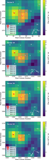 |
Fig. A.1 Target pixel file for TOI-672 (marked as a white cross) from TESS Sectors 9,10, 36, and 63 (top to bottom). Other Gaia DR3 sources within a limit of 6 Gaia magnitudes difference from TOI-672 are marked as red circles, and are numbered in distance order from TOI-672. The aperture mask is outlined and shaded in red. This figure was created with tpfplotter (Aller et al. 2020). |
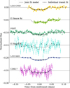 |
Fig. A.2 Photometry from various instruments described in Section 2.2, centred on the time from midtransit predicted by the joint fit model. From top to bottom, in chronological order: LCO CTIO (yellow circles); El Sauce Rc (green, offset by -0.05 in flux); PEST (sea green, offset by -0.10); El Sauce B (turquoise, offset by -0.15); LCO SSO (blue, offset by -0.20); and CDK17 (orchid, offset by -0.25). The photometry is binned as darker circles. The planet model from the joint fit using the TESS limb darkening is overlaid (dark grey solid lines), alongside the individual fits to each transit from the TTV search described in Section 5.5 for the LCO CTIO, PEST, LCO SSO, and CDK17 photometry (dashed black lines). The different models generally agree well, with a slight difference in transit “dip” shape caused by the difference in limb darkening parameters between the fits. |
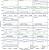 |
Fig. A.3 Photometry from ExTrA described in Section 2.2.2, where each panel is from a single observation night which is labelled. In each panel, observations can come from Telescope 1 (T1, top row, overall offset by +0.075 in flux), Telescope 2 (T2, middle row, no overall offset in flux), and/or Telescope 3 (T3, bottom row, overall offset by -0.075 in flux). For each telescope, we display the extracted photometry (pale grey dots, offset by +0.02 in flux) which is detrended by a GP (green line), to produce the detrended photometry (medium grey dots, no offset in flux), and then the individual transit model (purple line) is subtracted to show the residuals (dark grey dots, offset by -0.02 in flux). We also show the transit model from the joint fit (dashed black line, using the ExTrA limb darkening), which generally agrees well with the individual transit fits performed for the TTV search (purple line), see Section 5.5. |
All photometric transits of TOI-672 presented in this paper.
Appendix B Spectroscopic time series
NIRPS radial velocities extracted using LBL (version 0.65.006), using NIRPS observations of GJ 2066 to create the ‘friend’ template.
HARPS radial velocities reduced using the standard offline HARPS data reduction pipeline (DRS 3.5), using an M2 mask.
HARPS radial velocities extracted using LBL (version 0.65.006), using HARPS observations of TOI-776 to create the ‘friend’ template.
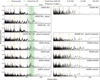 |
Fig. B.1 Lomb-Scargle periodograms (black lines) of the NIRPS (left column) and HARPS (right column) data. The best-fit period of TOI-672 b is shown (solid vertical orange line), along with its aliases (dashed orange lines). The recurrence timescale fit by the GP used on the NIRPS data (solid vertical green lines) is shown, along with the 1 standard deviation error (shaded green), and half the recurrence timescale (dashed vertical green line). The 0.1, 1, and 10% False Alarm Probabilities (FAPs, solid horizontal lines from dark to light grey) are calculated using the approximation from Baluev (2008). We describe the panels from top to bottom. First row: the RVs prior to detrending, clearly showing signals above the 0.1 % FAP thresholds at the planetary period (and its aliases). Second row: the NIRPS RVs with the planet signal removed. Third row: the NIRPS RVs detrended with the GP, where the significance of the planet signals has increased. Fourth row: the residual RVs after detrending (only in the case of the NIRPS RVs) and subtraction of the planet model, showing no further significant signals. Fifth to eighth rows: the dTemp, dLW, FWHM, and contrast activity indicators, respectively (all activity indicators are described in Section 2.4). None of the indicators show peaks at the planetary period. The NIRPS dTemp, dLW, and FWHM show a peak around 20 days of some significance (discussed in Section 3.3), and corresponding peaks at 20 days do also appear in all the HARPS activity indicators, though they are not significant. |
Appendix C Stellar analysis
Lines used for calculating the stellar elemental abundances of TOI-672.
Stellar elemental abundances of TOI-672.
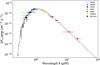 |
Fig. C.1 Spectral energy distribution of TOI-672, described in Section 3.1.4, assembled from broadband photometry obtained with APASS (magenta), SDSS (black), Gaia (green), 2MASS (yellow), WISE (red), and the Johnson system (blue). The horizontal bars indicate the effective wavelength ranges of each filter. The SED is fitted with a BT-Settl atmospheric model (Allard et al. 2012). |
Appendix D Joint fit priors and fit values
Prior distributions used in our joint fit model and the resulting fit values.
Appendix E Planet sample for Neptunian desert boundary study
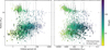 |
Fig. E.1 The sample used for the study of the Neptunian desert boundaries, described in Section 6 and given in Table E.1. |
Sample used for the study of the Neptunian desert boundaries.
All Tables
NIRPS radial velocities extracted using LBL (version 0.65.006), using NIRPS observations of GJ 2066 to create the ‘friend’ template.
HARPS radial velocities reduced using the standard offline HARPS data reduction pipeline (DRS 3.5), using an M2 mask.
HARPS radial velocities extracted using LBL (version 0.65.006), using HARPS observations of TOI-776 to create the ‘friend’ template.
All Figures
|
Fig. 1 Period-radius diagram showing TOI-672 b (yellow star) against the known planet population (light grey dots). Data of the known planet population are from the NASA exoplanet archive2, and only those with periods and radii determined to better than 4σ are shown. The background is also shaded according to this population. Planets around M dwarf hosts are highlighted (as green circles with a black outline, cut on Teff < 3900K, M*, R* < 0.6 M⊙, R⊙). The Neptunian desert boundaries derived by Mazeh et al. (2016) (orange line) and Castro-González et al. (2024) (red line) are shown. The desert, ridge, and savanna, as defined by Castro-González et al. (2024), are labelled, and the higher-period cut-off of the ridge is shown (dashed red line). |
| In the text | |
|
Fig. 2 TESS photometry for TOI-672 covering Sectors 9, 10, 36, and 63 (left to right, chronologically). The data are described in Section 2.1, and the fit to these data is described in Section 4.1. Top panel : PDCSAP flux (grey circles) and the GP model (green line) used for detrending. Middle panel : detrended flux after the GP model is subtracted and with the transit model shown (orange line). Bottom panel : residuals left after the GP and transit models are subtracted from the photometry. |
| In the text | |
|
Fig. 3 Top panel : detrended TESS photometry for TOI-672 from all sectors (grey circles, binned as dark brown circles) phase folded on the best-fit planetary period and with the transit model shown (orange line). Bottom panel: residuals after the GP and planet models are subtracted from the photometry. |
| In the text | |
|
Fig. 4 ExTrA photometry for TOI-672 from the night of 27 April 2024 using Telescope 2 (T2). The data are described in Section 2.2.2, and the fit to these data is described in Section 4.2. Top panel : extracted photometry (grey circles, binned as dark purple circles) and the GP model used to detrend it (green line). Middle panel : detrended photometry showing the transit model (purple line). Bottom panel residuals after the GP and transit models are subtracted from the photometry. |
| In the text | |
|
Fig. 5 Data from NIRPS and HARPS for TOI-672. The data are described in Section 2.4, and the fit to these data are described in Section 4.3. Top panel : NIRPS RVs (red triangles), the GP model fit to the NIRPS RVs (green line, with the one and two standard deviations of the fit shaded), and the combined GP and planet model (grey line). The BERV crossing event described in Section 2.4 is shaded in blue. Middle panel : both sets of RVs. Here, NIRPS has been detrended with a GP, and HARPS (blue circles) has no detrending. The planet-only model is shown with a grey line. Bottom panel : radial velocity residuals after the GP and planet models have been subtracted. |
| In the text | |
|
Fig. 6 Top panel : detrended NIRPS and HARPS RVs (red triangles and blue circles, respectively) phase-folded on the best-fit planetary period. The planet model is shown with a grey line, while the grey shading represents the one (darker) and two (lighter) standard deviations of the fit. Bottom panel : radial velocity residuals after the GP and planet model have been subtracted. |
| In the text | |
|
Fig. 7 Normalised NIRPS spectrum of TOI-672 (black line) compared to PHOENIX ACES stellar models (coloured lines). The models are described in Section 3.1.1. Top row : models with a fixed metallicity of −0.3 dex and Teff values of 3720 (blue), 3820 (orange), and 3920 (green) K for two spectral regions. Bottom row: same regions, but we show models with a fixed Teff of 3820 K and metallicity values of −0.5 (red), −0.3 (purple), and −0.1 (brown) dex. For strong spectral lines, we performed χ2 minimisation between the NIRPS spectrum and a grid of PHOENIX ACES models, finding Teff = 3810 ± 33 K and [M/H]=−0.3 ± 0.1 dex. |
| In the text | |
|
Fig. 8 Lomb-Scargle periodograms of the V band (top panel) and g′ band (bottom panel) photometry from ASAS-SN. The photometry are described in Section 3.3. The period of the highest peak is highlighted by a dash-dot green line, and it likely corresponds to the stellar rotation period. |
| In the text | |
|
Fig. 9 Mass-radius diagrams showing TOI-672 b (yellow star) against the well-characterised planet population (light grey dots) from the PlanetS catalogue, available at https://dace.unige.ch/exoplanets. It contains planets with precisions on planet mass and radius of <25 and 8%, respectively (Otegi et al. 2020; Parc et al. 2024). Planets around M dwarf hosts (i.e. Teff < 3900 K and M*, R* < 0.6 M⊙, R⊙) are highlighted as dark grey dots. Solar System planets are shown for comparison (outlined circles, labelled). Both panels show mass-radius relations from Skinner et al. (2026) for Earth-like rocky (32.5% core + 67.5% mantle) compositions (dark brown) and pure rock (100% mantle) compositions (light brown). Both panels also show model mass-radius relations from Skinner et al. (2026) (solid lines), as described in Section 5.2 for an equilibrium temperature of 700 K, with annotated percentages reporting the hydrogen mass fraction of each curve. The mass-radius relations in the left panel correspond to an Earth-like core composition (i.e. 32.5% iron + 67.5% mantle), while the right panel assumes a 50% water plus 50% Earth-like core composition. |
| In the text | |
|
Fig. 10 JADE exploration of TOI-672 b atmospheric evolution, assuming ages of 1, 5, and 10 Gyr (top, middle, and bottom rows, respectively). Left column : probability density function of the initial planet mass. The median is highlighted as an orange line, and the 1σ HDI interval is shown as dashed blue lines. Middle column : temporal evolution of the planet envelope mass in the best-fit simulation (orange curve) and a set of simulations from within the HDI interval (blue curves). The vertical black line with a grey shaded band marks the assumed age and uncertainties. Right column : same as the middle panel, but for the planet radius. The black point indicates the measured value. |
| In the text | |
|
Fig. 11 Sensitivity of the RV data, specifically the NIRPS data (top panel), HARPS data (middle panel), and combined NIRPS plus HARPS data (bottom panel), to additional planets orbiting TOI-672 as a function of planet mass and orbital period (using 50 × 50 bins in this parameter space). The calculation is described in Section 5.4. The sensitivity is shaded as in the colour bar, from 0 (dark purple) to 1 (light yellow). The 90 and 10% sensitivity limits are denoted by the dark purple and medium purple solid lines, respectively, and labelled in the top panel. The RV semi-amplitudes of 20, 10, 5, and 1 m s−1 are denoted by the red, orange, yellow, and white dashed lines, respectively, and labelled in the top panel. TOI-672 b is shown by the star marker (where error bars are too small to be seen). The habitable zone defined by Kopparapu et al. (2013), specifically the moist greenhouse inner edge and the maximum greenhouse outer edge calculated for the specific host star TOI-672, is shaded with a turquoise colour. |
| In the text | |
|
Fig. 12 Searching for TTVs in the transits of TOI-672b. Mid-transit times from fits to each individual transit (described in Section 5.5) are compared to the linear ephemeris from the joint fit model (i.e. the dark grey line at y = 0 in this plot, where the 1, 2 and 3 standard deviations from the value are shaded). The TESS transits are shown as orange circles; the LCO CTIO transit is the yellow triangle; the PEST transit is the green pentagon; the LCO SSO transit is the blue upside down triangle; the ExTrA transits are purple squares; and the Deep Sky Chile CDK17 transit is the orchid coloured diamond. |
| In the text | |
|
Fig. 13 Study of the Neptunian desert boundaries for FGK planet hosts versus M dwarf hosts in period-radius space, as described in Section 6. Our planet sample (Table E.1; Fig. E.1) is shown as coloured dots, according to the weighting of each planet. In the top panel, our full planet sample is shown (where M dwarf hosts are highlighted with black outlines). The middle panel shows planets around FGK hosts only, and the bottom panel shows planets around M dwarf hosts. The boundaries of the bins in radius space are depicted with dashed lines and the bins are numbered 1-8 in the top panel. The period percentile values calculated for each bin and their errors are shown. The 2.3-97.7 percentiles are shaded in light grey, while the 16-84 percentiles are shaded in dark grey. |
| In the text | |
|
Fig. 14 Study of the Neptunian desert boundaries for FGK planet hosts versus M dwarf hosts in instellation-radius space, as described in Section 6. The details are the same as in Fig. 13. |
| In the text | |
|
Fig. 15 Comparison of the Neptunian desert boundaries in periodradius space as derived by Mazeh et al. (2016) (yellow dotted lines), Castro-González et al. (2024) (orange dashed lines), and this work, where we calculated the desert boundaries for FGK planet hosts (grey solid line) and M dwarf hosts (black solid line) separately. The background is shaded according to the known planet population from the NASA exoplanet archive, as in Fig. 1. |
| In the text | |
|
Fig. 16 Comparison of the Neptunian desert boundaries in instellation-radius space as derived in this work, where we calculated the desert boundaries for FGK planet hosts (grey solid line) and M dwarf hosts (black solid line) separately. The background is shaded according to the known planet population from the NASA exoplanet archive, as in Fig. 1. |
| In the text | |
|
Fig. A.1 Target pixel file for TOI-672 (marked as a white cross) from TESS Sectors 9,10, 36, and 63 (top to bottom). Other Gaia DR3 sources within a limit of 6 Gaia magnitudes difference from TOI-672 are marked as red circles, and are numbered in distance order from TOI-672. The aperture mask is outlined and shaded in red. This figure was created with tpfplotter (Aller et al. 2020). |
| In the text | |
|
Fig. A.2 Photometry from various instruments described in Section 2.2, centred on the time from midtransit predicted by the joint fit model. From top to bottom, in chronological order: LCO CTIO (yellow circles); El Sauce Rc (green, offset by -0.05 in flux); PEST (sea green, offset by -0.10); El Sauce B (turquoise, offset by -0.15); LCO SSO (blue, offset by -0.20); and CDK17 (orchid, offset by -0.25). The photometry is binned as darker circles. The planet model from the joint fit using the TESS limb darkening is overlaid (dark grey solid lines), alongside the individual fits to each transit from the TTV search described in Section 5.5 for the LCO CTIO, PEST, LCO SSO, and CDK17 photometry (dashed black lines). The different models generally agree well, with a slight difference in transit “dip” shape caused by the difference in limb darkening parameters between the fits. |
| In the text | |
|
Fig. A.3 Photometry from ExTrA described in Section 2.2.2, where each panel is from a single observation night which is labelled. In each panel, observations can come from Telescope 1 (T1, top row, overall offset by +0.075 in flux), Telescope 2 (T2, middle row, no overall offset in flux), and/or Telescope 3 (T3, bottom row, overall offset by -0.075 in flux). For each telescope, we display the extracted photometry (pale grey dots, offset by +0.02 in flux) which is detrended by a GP (green line), to produce the detrended photometry (medium grey dots, no offset in flux), and then the individual transit model (purple line) is subtracted to show the residuals (dark grey dots, offset by -0.02 in flux). We also show the transit model from the joint fit (dashed black line, using the ExTrA limb darkening), which generally agrees well with the individual transit fits performed for the TTV search (purple line), see Section 5.5. |
| In the text | |
|
Fig. B.1 Lomb-Scargle periodograms (black lines) of the NIRPS (left column) and HARPS (right column) data. The best-fit period of TOI-672 b is shown (solid vertical orange line), along with its aliases (dashed orange lines). The recurrence timescale fit by the GP used on the NIRPS data (solid vertical green lines) is shown, along with the 1 standard deviation error (shaded green), and half the recurrence timescale (dashed vertical green line). The 0.1, 1, and 10% False Alarm Probabilities (FAPs, solid horizontal lines from dark to light grey) are calculated using the approximation from Baluev (2008). We describe the panels from top to bottom. First row: the RVs prior to detrending, clearly showing signals above the 0.1 % FAP thresholds at the planetary period (and its aliases). Second row: the NIRPS RVs with the planet signal removed. Third row: the NIRPS RVs detrended with the GP, where the significance of the planet signals has increased. Fourth row: the residual RVs after detrending (only in the case of the NIRPS RVs) and subtraction of the planet model, showing no further significant signals. Fifth to eighth rows: the dTemp, dLW, FWHM, and contrast activity indicators, respectively (all activity indicators are described in Section 2.4). None of the indicators show peaks at the planetary period. The NIRPS dTemp, dLW, and FWHM show a peak around 20 days of some significance (discussed in Section 3.3), and corresponding peaks at 20 days do also appear in all the HARPS activity indicators, though they are not significant. |
| In the text | |
|
Fig. C.1 Spectral energy distribution of TOI-672, described in Section 3.1.4, assembled from broadband photometry obtained with APASS (magenta), SDSS (black), Gaia (green), 2MASS (yellow), WISE (red), and the Johnson system (blue). The horizontal bars indicate the effective wavelength ranges of each filter. The SED is fitted with a BT-Settl atmospheric model (Allard et al. 2012). |
| In the text | |
|
Fig. E.1 The sample used for the study of the Neptunian desert boundaries, described in Section 6 and given in Table E.1. |
| In the text | |
Current usage metrics show cumulative count of Article Views (full-text article views including HTML views, PDF and ePub downloads, according to the available data) and Abstracts Views on Vision4Press platform.
Data correspond to usage on the plateform after 2015. The current usage metrics is available 48-96 hours after online publication and is updated daily on week days.
Initial download of the metrics may take a while.