| Issue |
A&A
Volume 709, May 2026
|
|
|---|---|---|
| Article Number | A181 | |
| Number of page(s) | 19 | |
| Section | Galactic structure, stellar clusters and populations | |
| DOI | https://doi.org/10.1051/0004-6361/202555519 | |
| Published online | 13 May 2026 | |
The evolution of velocity dispersion in the Sco-Cen OB association
1
Astronomical Institute of the Czech Academy of Sciences,
Boční II 1401,
141 31
Prague 4,
Czech Republic
2
Universität zu Köln, I. Physikalisches Institut,
Zülpicher Str. 77,
50937
Köln,
Germany
3
University of Vienna, Department of Astrophysics,
Türkenschanzstraße 17,
1180
Vienna,
Austria
4
University of Vienna, Data Science at Uni Vienna Research Platform,
Austria
5
Center for Astrophysics I Harvard & Smithsonian,
60 Garden St.,
Cambridge,
MA
02138,
USA
6
Departament de Física Quàntica i Astrofísica (FQA), Univ. de Barcelona (UB),
Martí i Franquès, 1,
08028
Barcelona,
Spain
7
Institut de Ciències del Cosmos (ICCUB), Univ. de Barcelona (UB),
Martí i Franquès, 1,
08028
Barcelona,
Spain
★ Corresponding author: This email address is being protected from spambots. You need JavaScript enabled to view it.
Received:
14
May
2025
Accepted:
4
March
2026
Abstract
We study how the stellar velocity dispersion within the Scorpius-Centaurus OB association (Sco-Cen) has evolved over approximately 20 million years, from its formation to the present day, by investigating 32 stellar clusters in Sco-Cen. Using data from the Gaia mission along with supplementary stellar radial velocities, we identified a surprising sequence of abrupt jumps and intervening plateaus in the evolution of velocity dispersion correlating with times of star formation bursts. We find that the association is almost isotropically expanding and that star formation propagated from inside-out with a speed of about 5-6 km s−1. We measure a present-day expansion rate of about 10-12 pc Myr−1 and observe that younger star clusters within the association exhibit higher velocities compared to older ones. This result, along with the stepwise increase in velocity dispersion over time, suggests a structured and sequential star formation process rather than a random one. This phased evolution suggests that stellar feedback is the primary driver of Sco-Cen’s star formation history, expansion, and eventual dispersal. Our findings emphasise the value of precisely characterising stellar populations within OB associations, particularly through the creation of detailed, high-resolution age maps.
Key words: astrometry / parallaxes / proper motions / time / stars: kinematics and dynamics / open clusters and associations: individual: Sco-Cen
© The Authors 2026
 Open Access article, published by EDP Sciences, under the terms of the Creative Commons Attribution License (https://creativecommons.org/licenses/by/4.0), which permits unrestricted use, distribution, and reproduction in any medium, provided the original work is properly cited.
This article is published in open access under the Subscribe to Open model. This email address is being protected from spambots. You need JavaScript enabled to view it. to support open access publication.
1 Introduction
Understanding the temporal evolution of OB associations is important to gain insights into the role of massive stars in shaping their environments (e.g. Brown et al. 1997). OB associations represent an essential yet transient phase in the life cycle of massive stars and star-forming regions (e.g. Blaauw 1964a; Wright et al. 2023). The traditional view of OB associations has been significantly refined with Gaia data (Gaia Collaboration 2016). Recent Gaia-based studies reveal that OB associations comprise dozens of largely unbound stellar populations with ages of up to roughly 20 Myr (e.g. Kos et al. 2019; Chen et al. 2020; Kerr et al. 2021; Ratzenböck et al. 2023b; Hunt & Reffert 2023), rather than just a few subgroups. Moreover, they are likely linked to even larger and older cluster families, the origins of which can be traced to spiral arm activity (Swiggum et al. 2024, 2025).
A comprehensive characterisation of stellar groups within OB associations is crucial for understanding their formation mechanisms and boundness state, as they ultimately disperse and merge with the field star population (e.g. Lynga & Palous 1987; Kamaya 2004). OB associations also provide insights into star formation mechanisms, stellar feedback, and early dynamical evolution. Their velocity dispersion is a key factor that provides insights into the internal motions, dynamical states, and evolutionary histories of stellar populations, eventually shaping the structure of the Galactic field population (e.g. Lada et al. 1984; Lada & Lada 2003; Kroupa 1995, 2008; de la Fuente Marcos & de la Fuente Marcos 2008; Kuhn et al. 2019).
Although velocity dispersion is widely recognised as a fundamental population property, its temporal evolution during the formation of a single stellar association remains largely unexplored. Previous observational studies provide only snapshots in time, which limit our understanding of how stellar populations evolve dynamically. The lack of observational data on the temporal evolution of velocity dispersion represents a major gap in our understanding of stellar population formation.
To address this, we used high-precision Gaia DR3 data (Gaia Collaboration 2023), supplemented with ancillary radial velocity (RV) measurements, to investigate the temporal evolution of velocity dispersion in the Scorpius-Centaurus OB association (Sco-Cen; e.g. Blaauw 1964a,b; Preibisch & Mamajek 2008). This study builds on the recent identification of more than 30 coeval and comoving stellar clusters1 within Sco-Cen with ages of approximately 3 to 21 Myr (see Ratzenböck et al. 2023a,b; Miret-Roig et al. 2025, hereafter, R23a, R23b, MR25). These studies identified spatio-temporal patterns, using highresolution age maps, indicative of sequential star formation. This enabled the identification of cluster chains with a well-defined age, mass, position, and velocity gradients extending outwards at the periphery of the association (see Posch et al. 2023, 2025, hereafter, P23, P25). In this paper, we aim to reconstruct, for the first time, the temporal evolution of velocity dispersion and internal motions of an OB association by analysing 32 well-defined clusters in the 6D phase space over a time span of about 20 Myr.
2 Data
We used the Sco-Cen cluster sample from R23a, which was selected using the unsupervised machine-learning tool SigMA (Significance Mode Analysis), containing 34 clusters related to Sco-Cen. We added two clusters from the TW Hydrae association (TWA), which are connected to Sco-Cen as a cluster chain (see MR25). The combined sample contains a total of 13 011 stellar members. R23b determined cluster ages by fitting PARSEC model isochrones (Bressan et al. 2012) with a Bayesian inference approach. We used the isochronal ages fitted to the Gaia colour-absolute-magnitude diagram Gabs versus GBP - GRP (BPRP-PARSEC ages). MR25 estimated the cluster ages of TWA-a,b consistently with the same method as R23b. The Sco-Cen clusters cover ages from about 3 to 21 Myr, and were used as time information in our analysis. A detailed data description is given in Appendices A.1 and A.2.
To study the clusters in 6D phase space, we combined the astrometric 5D data with RV data. Gaia DR3 provides RV measurements (Katz et al. 2023) for about 38% of our sources; however, only about 11% have relatively low uncertainties (eRV,Gaia < 3.1 km s−1)2 with a median error of about 1.5 km s−1. Moreover, some of the relatively sparse clusters contain no or very few stars with Gaia RVs. Hence, we added supplementary RV data from 22 spectroscopic surveys (see Appendix A.3 and Table A.1). After the cross-match, about 50% of the sources have RV measurements from at least one survey. To determine robust 3D space motions, we applied several cleaning steps, including a cut using the cluster stability value from R23a, an RV error cut at eRV < 3.1 km s−1, removal of binary candidates, and a global outlier cut and 3σ-clipping, as is outlined in detail in Appendix A.4. Finally, our RV sample contains about 25% of the original stellar sample (3240/13 011). The median RV error of this sample is about 0.4kms−1 (min/max = 0.010/3.098 kms−1). A detailed overview of the data statistics per cluster is given in Table A.2.
Eventually, we used 32 out of the 36 Sco-Cen clusters. We find that the sparse cluster μ Sco has very poor RV statistics, and we removed it from further analysis in this work. Moreover, we removed three clusters from the Chamaeleon-Musca-Coalsack region (Chamaeleon I and II, Centaurus-Far). They are slightly detached from Sco-Cen and probably belong to a background structure, called ‘The C’ (Edenhofer et al. 2024b). The remaining 32 analysed clusters contain a total of 12612 stellar candidate members (containing 3123 sources with valid RVs), while we also report statistics for the four removed clusters in Table A.2.
3 Methods
We calculated the velocity dispersion from the stellar members of the clusters in 3D, using the Galactic Cartesian velocities (UVW; see Appendix A.2), after applying the quality criteria from Appendix A.4:
 (1)
(1)
The one-dimensional velocity dispersions (σU, σV, σW) were calculated via the standard deviation in the three velocity spaces. We used the cluster ages as time information to investigate the evolution of velocity dispersion in 3D. This is possible for the first time, as we have a coherent sample of clusters that formed in a single OB association with a wide range of ages and with 3D information.
We calculated σ3D cumulatively by progressively incorporating member stars of the next youngest cluster at each time step for its calculation. In other words, we started the calculation of the cumulative σ3D with only the stellar members of the oldest cluster (e Lup), then added the stars of the next youngest cluster at the next step, and finally we ended with all member stars from all studied 32 clusters. We calculated the cumulative σ3D by iteratively picking equal subsamples from each cluster at each step, to account for the different cluster sizes (number of stellar members), as is detailed in Appendix B.1.
Next, we estimated the present-day spatial arrangement of the clusters in Sco-Cen in chronological order by ordering the clusters by age, named cumulative size (S, pc). To this end, we determined the maximum cluster extent as observed today by measuring the minimal distance across the connections using a k-nearest neighbour graph of the member stars in the XYZ space. We constructed this graph from individual stellar members as nodes, and we used Dijkstra’s algorithm to compute the shortest paths between any two sources along the edges of this graph. We did this cumulatively again by starting with member stars from the oldest cluster and ending with all member stars. Thus, at each step, we computed the maximally possible path distance that one can take between any two pairs of Sco-Cen member stars older than the given age step. More details are given in Appendix B.2.
The present-day cumulative S calculated here does not reflect the evolution of size over time, since we do not include orbital tracebacks of the clusters at this stage, but only order the clusters by their decreasing age. The cumulative sizes calculated in this manner can be interpreted as an upper limit of the region’s size at a given age (‘time’), while it does not show the true physical extent before the present day, which was likely smaller. We shall look into a more detailed traceback analysis in a future work, in which various second-order effects and required assumptions will be taken into account (e.g., cluster expansion, unknown acceleration from feedback, non-sphericity, Galactic potential, possible internal gravitational effects, and orbit integration with different solar parameters; see Sect. 5.4).
We further investigated the clusters’ 3D bulk positions and motions, using the cluster medians in Galactic Cartesian coordinates (XYZ) and velocities (UVW). The corresponding uncertainties were determined by bootstrap sampling from the cluster members (Appendix B.3). We calculated the position and velocity vectors for each cluster relative to a chosen centre (XYZctr) and rest velocity (UVWrest):
 (2)
(2)
Next, we calculated the relative distances of the clusters (r, vector norm, in parsecs) and the relative velocities (v, or speed, in km s−1), via the Euclidean distance in position and velocity space to the given reference point.
 (3)
(3)
We determined the radial component of the velocities relative to the chosen reference point as follows:
 (4)
(4)
The tangential component was then computed with
 (5)
(5)
To define the reference point (centre and rest velocity), we used three approaches to investigate possible systematics. The centre of Sco-Cen is not a well-defined point and depends also on the question at hand (e.g., centre of feedback, centre of mass, or using older clusters to find the point of first star formation). First, we used the median position and motion of the oldest cluster in the region, e Lup (age ∼21 Myr), which is located at a central position. We assumed that its velocity is reminiscent of the original velocity of the primordial star-forming molecular cloud when the first stars formed. Additionally, we used the cluster φ Lup, another central cluster in Sco-Cen with an age of ∼17Myr, which is connected to two chains of clusters (see P23; P25). Finally, we used the median motion of the stellar members of the oldest clusters in Sco-Cen with ages of > 15 Myr, denoted as SC15, to get another estimate of the bulk motion of the early star-forming region (see similar approaches in P25 and MR25). More details on the determination of SC15 and a comparison of the three chosen centres (e Lup, φ Lup, SC15) are given in Appendix B.4.
We further investigated the biasing effects from choosing different reference points in our subsequent analysis by using each of the 32 Sco-Cen clusters once as a reference point. This created cases that are not ordered by cluster age or that start from a non-central location, as is detailed in Appendix B.5.
4 Results
4.1 Cumulative velocity dispersion
Figure 1 shows the cumulative 3D velocity dispersion (σ3D) of Sco-Cen as a function of cluster age (or lookback time). We observe a general increase in velocity dispersion over time, with a pattern of jumps and plateaus, reaching a final value of 4.64±0.04kms−1. This cumulative value was determined by iterating over equally sized sub-samples within each cluster (see details in Appendix B.1). For comparison, the total σ3D, calculated using all stellar members of Sco-Cen that meet our quality criteria (without sub-sampling), yields a value of 3.97±0.03 kms−1. The different values of the total 3D velocity dispersion are caused by the sub-sampling approach that we used for the cumulative σ3D, to give similar weight to each cluster, while in the case when using all available stars, the more massive clusters might dominate the total σ3D. Moreover, the iterative sub-sampling approach likely creates some undersampling of the velocity space, which gives more weight to individual measurement errors, artificially inflating the velocity dispersion, while the shape of the cumulative trend appears unaffected, as is demonstrated in the following paragraph and in more detail in Appendix B.1.
We tested the shape and robustness of the cumulative trend by calculating the cumulative σ3D, first by applying stricter error cuts (eRy < 1 kms−1) and second by using the UVW medians of the 32 clusters instead of individual stars. In the first case, we get a total velocity dispersion of 4.46±0.03kms−1, and in the second case 4.13±0.06kms−1. Additionally, we tested the effect of binaries that might be contained in our sample, using the Gaia RUWE parameter to roughly exclude binary candidates, which results in effectively the same trend as in Fig. 1. Generally, all tests produce similar increasing trends of the cumulative σ3D over time, while only the magnitude of σ3D gets shifted (see Appendix B.1 and Fig. B.1)
We conclude that the whole Sco-Cen association has a 3D velocity dispersion of about 4-4.7 km s−1 (see Table B.1), whereas individual clusters within the association have significantly smaller dispersions, of the order of 1-2km s−1 per cluster3. We find that the shape of the cumulative σ3D is largely unaffected by measurement errors or binaries, since only the magnitude of the σ3D values shifts consistently to lower values when applying more conservative cuts (see Fig. B.1).
Figure 2 highlights the present-day 3D distribution of the Sco-Cen clusters and shows which clusters contribute to the patterns in the cumulative σ3D. This figure visualises the arrangement of Sco-Cen clusters at seven age ranges, systematically including younger clusters. The cluster positions in 3D represent the present-day locations, since we do not consider orbital tracebacks, which will be considered in future work to better understand the true spatial evolution of Sco-Cen. Hence, the shown cluster sizes can be interpreted as upper limits of the region’s size at a given age and not as the true physical extent before the present-day, which was likely smaller (see also Sect. 5.4). Nevertheless, already in the visualisation shown in Fig. 2 it becomes clear that the increasing velocity dispersion within Sco-Cen is connected to an evolutionary pattern, from the inside out. Changes in σ3D likely appear when star formation proceeds to an adjacent gas reservoir; notably, the onset of the formation of the cluster chains correlates with an increase and jump in σ3D. To further investigate the origin of the increase in the velocity dispersion during the evolution of Sco-Cen, we look in more detail into the relative 3D space motions and positions of the Sco-Cen clusters in the following Sect. 4.2.
To quantify the age-ordered, inside-out patterns visible in the 3D distribution of clusters in Fig. 2, we calculated Sco-Cen’s size chronologically in a cumulative manner. Figure 3 shows the present-day cumulative size (S, pc); hence, it highlights the cumulative chronological arrangement of Sco-Cen clusters, when ordering and adding the member stars by the age of their parent clusters, calculated cumulatively with decreasing cluster age. We like to emphasise that the presented trend does not show the evolution of size, since we do not consider orbital tracebacks at this stage. Thus, as was mentioned above, the presented sizes at given ages can rather be seen as upper limits, since the region was likely more compact in the past, based on a preliminary traceback analysis (see Sect. 5.4). The total present-day extent of Sco-Cen is  pc, when calculated with the method described in Appendix B.2 and when including all clusters. The size increases when adding stars from clusters ordered by decreasing age, which is consistent with the visible spatio-temporal patterns identified in R23b (Fig. 2) and the cluster chains discussed in P23, P25, and MR25. These studies propose an inside-out formation history, which was also suggested earlier for Sco-Cen (e.g. Preibisch & Zinnecker 1999; Gaczkowski et al. 2017; Krause et al. 2018). Interestingly, we see that the present-day cumulative size increases similarly to the cumulative σ3D, which we discuss further in Sect. 5.4.
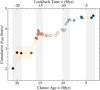 |
Fig. 1 Cumulative 3D velocity dispersion of Sco-Cen, ordered by decreasing cluster age. The shaded orange area shows the 95% interquartile ranges (2σ bound), highlighting the uncertainties of the trend (see Appendix B.1). The symbols are coloured by the formation time of the youngest cluster included in the cumulative calculation (colour correlates with x-axis). We indicate the lookback time at the top of the x-axis, since the cumulative σ3D could also be interpreted as the evolution of velocity dispersion over time. The four vertical grey bars indicate the four main star formation events in Sco-Cen, marking four periods of an increased star formation rate, as is discussed in R23b (see their Fig. 3). |
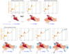 |
Fig. 2 3D spatial distribution of clusters in Sco-Cen together with the cumulative σ3D. The seven panels show seven age ranges, which dissect the chronological build-up of Sco-Cen. The upper panels display the cumulative 3D velocity dispersion (as in Fig. 1). Below each graph, seven 3D age maps depict the present-day spatial distribution of clusters (in XYZ). The clusters are represented by their enveloping surfaces and colour-coded by age. Each of the seven panels only shows the clusters that formed before the indicated cluster formation times. The shown cluster sizes can be interpreted as upper limits of the region’s size at a given age and not as the true physical extent before the present-day, which was likely smaller (see Sect. 5.4). The figure illustrates which clusters contribute to which jumps or steps in the cumulative σ3D. Sub-regions and cluster chains are labelled in the final panel. The 3D visualisations originate from R23b and MR25; interactive versions are available in the respective publications. |
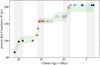 |
Fig. 3 Present-day cumulative size of Sco-Cen, when ordering and adding the stellar cluster members by their decreasing age (without considering orbital trace-backs). The sizes can be seen as upper limits of the region’s size at a given age, but not as the true physical extent before the present-day, which was likely smaller (see Sect. 5.4). The shaded green area shows the 95% interquartile range (2σ; see Appendix B.2). The colours and grey bars are as in Fig. 1. |
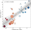 |
Fig. 4 Speed-time relation. Relative cluster speed (v) versus lookback time (t), with the oldest cluster (e Lup) as a reference point that is excluded from the linear fit (dashed black circle). The symbols are colour-coded by formation time (or cluster age; see the x-axis) and scaled by number of sources per cluster. The linear fit (solid grey line) was obtained via bootstrapping, with the median fitting parameters given in the upper left corner. The fit uncertainties are plotted as shaded grey areas (1-2-3 σ). |
4.2 Correlation of time, cluster motion, and position
Figure 4 shows the cluster speed (v) versus the time of cluster formation (t), denoted as the look-back time, with the oldest cluster, e Lup, as a reference point. We find a linear relation between speed and time, with the resulting fitting parameters reported in Table 1. The slope of the relation is about 0.45 km s−1 Myr−1, where younger clusters have a systematically higher relative speed. The intercept gives about 11 pc Myr−1, which could be interpreted as expansion velocity at the present day. However, the speed calculated in this manner (Eq. (3)) does not give information about the direction of motion; therefore, we also dissected the relative motions into a radial and tangential component (Eqs. (4) and (5)).
Figure 5 shows the radial component of the relative cluster motions (vr) versus relative distance (r), again with e Lup as a reference point. First, we find that the majority of clusters have positive values in vr, which shows that most of them are moving away from the central cluster e Lup, while younger clusters tend to have higher radial outward motions. Only one of the older and the most massive clusters at the centre of Sco-Cen shows a slightly negative component, which is ν Cen with vr ~ −0.1 km s−1. Second, we find a clear linear trend, whereby vr increases with r. We fitted a linear regression to the data points, only using clusters with vr > 0 (excluding e Lup and ν Cen). This delivers a slope of about 0.09 km s−1 pc−1, named the radialmotion-distance relation (see Table 1). Hence, clusters at larger distances from the centre tend to have higher velocities radially away from it, suggesting an outward expansion, reminiscent of a Hubble flow. The inverse of the slope gives a time of about 11 Myr. This can be interpreted, to first order, as the approximate time of the onset of significant radial expansion, assuming no external forces.
We repeated the same analysis with two alternative reference frames - using φ Lup and SC15, instead of e Lup (see Sect. 3 and Appendix B.4) - to test the robustness of the identified relations. For these two cases, we find similar trends with slightly shallower slopes, showing that the expansion patterns are valid from different reference points that are located at central locations (see Fig. B.2 and Table 1).
We further tested the linear relations by setting each of the 32 clusters once as a reference point (see Appendix B.5). With this, we checked if the older clusters at central locations (such as e Lup or φ Lup) are likely a centre of expansion, or if the expansion pattern is independent of the central area or the age of the reference cluster (hence, independent of time). In most cases, the resulting correlations are less clear, showing more scatter and flatter slopes when compared to e Lup as a reference point. We also tested whether the radial motions of the clusters are positive for the majority of the test cases when using each cluster once as a reference point, since negative values indicate infalling motions. In some cases (mostly when using younger clusters as reference points), we find that several clusters now have negative vr, which means that those reference points appear to create relatively in-falling motions instead of predominantly expanding motions, which suggests that these clusters are less likely to be the point of expansion. These tests show us that, independent of the reference frame, the association appears to be expanding radially in most cases, in particular when using clusters with ages of > 12 Myr as a reference, while the cleanest trend is created when using e Lup (see more details in Appendix B.5).
To further test the statistical significance of the correlation of speed with time (Fig. 4), we randomised the order of the time axis, as is detailed in Appendix B.5. We find that the probability of obtaining a similar linear relation is below 4σ. In other words, random (not time-ordered) cases tend to produce shallower or reverse slopes and/or larger scatter. This suggests that the Sco-Cen clusters did not form randomly and independently from each other, but rather sequentially via propagated star formation.
Additionally, we explored the expansion patterns using three position-velocity diagrams (PVDs) in the three Cartesian directions, shown in Fig. 6. We used the clusters’ median positions, XYZ, and space motions relative to the local standard of rest (LSR), UVWLSR, named the XU, YV, and ZW diagrams. The XU and YV diagrams show positive correlations of position with velocity, which again suggests a large-scale expansion of the whole region. The ZW diagram shows more scatter and a less clear trend, while position and velocity are generally positively correlated. We fitted linear regressions to the data in the three spaces and report the medians and uncertainties in Table 2 (determined via bootstrapping).
Looking at the ZW diagram in more detail (right panel in Fig. 6), we find that some clusters appear to be outliers, located mainly in the Upper Scorpius (USco) region. The discrepancy in the motion of these clusters correlates with an additional tangential component of motion relative to the reference point, observed for seven clusters, which is discussed in more detail in Sect. 5.2. When we remove these seven clusters, we find a clearer correlation and expansion pattern in ZW, while the trends in XU and YV remain similar (see Fig. 6 and Table 2). Nevertheless, in Fig. 5 we find that the radial component of motion versus relative distance of these seven odd clusters follows the same trend as the rest of the Sco-Cen clusters.
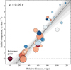 |
Fig. 5 Radial-motion-distance relation. Radial component of the relative cluster motions (vr) versus relative cluster distance (r), with e Lup as a reference point. The symbols are colour-coded by formation time, as in Fig. 4. A linear fit to the data is shown as a solid grey line, with the best-fitting slope given in the upper left corner, and the 1-2-3σ fit uncertainties are plotted as shaded grey areas. The two clusters marked by dashed black circles (e Lup, ν Cen) are excluded from the linear fit. |
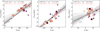 |
Fig. 6 Position velocity (PV) diagrams for the 32 Sco-Cen clusters using the XU, YV, and ZW spaces. Symbols and colours as in Fig. 4. The median slopes of the fitted linear regressions (solid black lines) are given in the upper left corners. The shaded grey areas are the 1-2-3σ uncertainty ranges. The inverse of the slope gives a time in million years, in brackets, marking the possible onset of expansion. The dashed red slopes are the linear fitting results when using only 25 clusters, after removing seven clusters with peculiar tangential motions, marked with red circles (see Sect. 5.2). In the ZW diagram (right panel), the vertical dashed grey line indicates the approximate location of the Galactic mid-plane, assuming that the Sun is located about 21 pc above the plane (e.g. Bennett & Bovy 2019). |
5 Discussion
In this paper, we present the first measurement of the temporal evolution of stellar velocity dispersion within a young stellar population. By using high-precision Gaia data supplemented with additional RV data, we identified an unexpected series of jumps and plateaus in the evolution of the velocity dispersion over the formation period of the Sco-Cen OB association (approximately 20 Myr). These findings suggest that star formation within Sco-Cen did not occur randomly but is structured and sequential. The simplest interpretation of our results suggests a scenario in which stellar feedback plays a significant role in influencing the observed dynamic evolution of stellar populations within the association.
The surprising sequence of abrupt jumps and intervening plateaus in the cumulative σ3D of the Sco-Cen association, the central finding of this paper, correlates with four distinct star formation bursts. The four periods of a heightened star formation rate, as identified in R23b, are marked by four vertical grey bars in Figs. 1, 2, and 3. These periods are separated by about 5Myr. These findings suggest a structured and sequential formation process for Sco-Cen, likely driven by stellar feedback. As is illustrated in Fig. 2, the jumps occur when star formation transitions spatially to an adjacent region, as is suggested by the present-day distribution of clusters. The observed jumps can be interpreted as the addition of a new ensemble of younger clusters; these additional young clusters have been formed from a nearby gas reservoir (close to the existing populations of stars) with a marginally different velocity.
The concept of bursts in star formation and the complex age structures within Sco-Cen have been a subject of extensive research in previous works. For instance, Slesnick et al. (2008) investigated the USco subgroup, concluding that its low-mass population formed in a single burst approximately 5 Myr ago, with an age spread of fewer than 3 Myr, after accounting for observational uncertainties. While this suggested a relatively coeval formation at the time, the apparent age spread observed in their Hertzsprung-Russell diagrams highlighted the complexities of age determination. More recently, Pecaut & Mamajek (2016) conducted a comprehensive study across all three traditional Sco-Cen subgroups, demonstrating that none of them is consistent with simple, coeval populations formed in single bursts. Instead, they found strong evidence for age gradients and a ‘multitude of smaller star formation episodes’ throughout the association, suggesting a more complex and prolonged star formation history, as has recently been confirmed, for instance, by R23b (see also the discussion in Sect. 5 in R23b). Pecaut & Mamajek (2016) emphasised the presence of substructure and found larger intrinsic age spreads (e.g. ±7 Myr for USco) when using revised age scales and accounting for various observational effects. Our current findings provide novel kinematic evidence for these multi-episodic or burst-like star formation events, demonstrating how these bursts manifest as distinct ‘stepwise’ increases in the collective velocity dispersion of the association over time. This directly reinforces the understanding that Sco-Cen’s evolution is not monolithic but rather a phased assembly of spatially and kinematically distinct stellar populations.
This sequential progression in space and time, characterised by radially ordered outward motions rather than random (Figs. 4 and 5), suggests the presence of a coordinating agent. A plausible agent to create the observed order in cluster positions, ages, and motions, particularly in a region of star formation known for producing massive stars, is stellar feedback. This mechanism can elucidate the inside-out arrangement of events, which is not easily reproduced. For instance, we find that the correlations break down if we arrange the clusters randomly and not by cluster age (formation time), or if we use other reference points instead of the older clusters that are largely located at central locations (see randomised trials in Appendix B.5). Furthermore, by effectively accelerating nearby gas reservoirs, the feedback scenario accounts for the observation that the youngest clusters exhibit the highest velocities relative to the older, more massive clusters (Fig. 4). This scenario has already been outlined for the four cluster chains, as is discussed in P23; P25, and in MR25, who find acceleration from older to younger clusters, with the youngest moving away the fastest from the centre of Sco-Cen. The simplest scenario that aligns with these observations posits that feedback from prior episodes of star formation compresses and accelerates adjacent gas reservoirs of the primordial Sco-Cen gas cloud, ultimately leading to the formation of new stars (e.g. de Avillez & Breitschwerdt 2005; Großschedl et al. 2021; P23; P25; Alves et al. 2025). This mechanism essentially embodies the Elmegreen & Lada (1977) scenario in action, which naturally ends when the capacity to compress molecular gas into collapsing dense cores is exhausted.
The plateaus observed in the cumulative velocity dispersion (Fig. 1) warrant further investigation. These plateaus are not perfectly flat and exhibit, on average, subtle increases in velocity dispersion between the transitions. In this context, plateaus suggest the presence of a relatively coherent reservoir of gas forming a group of clusters, analogous to ‘peas in a pod’ (see also Fig. 2). In this analogy, the jumps in σ3D over time can be seen as star formation transitioning into a new ‘gas pod’, at a slightly different average velocity, either primordial or, likely, affected by feedback. It remains to be studied how much of the next ‘pod’ was created by fragmentation of the primordial gas cloud and how much of it was assembled by feedback from the previous star formation episode. The CrA, LCC, and USco chains of clusters, representing the later stages of the formation of the association, clearly require a more dominant role for feedback, to be able to explain the observed accelerations (P23; P25; MR25). It seems reasonable to posit that the impact of feedback on the formation is not constant over the formation of an OB association, but is coupled to the simultaneous presence of massive stars and their feedback output.
The three to four periods of an enhanced star-formation rate found in the star formation history of Sco-Cen, as reported in R23b4, could be interpreted as observational evidence in support of the so-called ‘Type-I triggering’ discussed in Dale et al. (2015a). This type of star formation triggering, although posited to be theoretically unlikely, describes a temporal increase in the star formation rate, which is attributed to the presence of massive stars able to shape their environments, not unlike the scenario proposed above.
5.1 Expansion of Sco-Cen
Using Gaia DR1, Wright & Mamajek (2018) found no evidence of expansion in Sco-Cen. With Gaia DR3, we revisit this question by examining the relative motions of the 32 Sco-Cen clusters. This updated view of Sco-Cen covers a larger area than previous studies (such as Wright & Mamajek 2018), which allows us, together with the higher precision of Gaia DR3, to reinvestigate the internal motions of the region. We find clear evidence for expansion, with a present-day speed of about 10pcMyr−1, which likely started around 11-14Myr ago (Figs. 4-5, Table 1). Similar expansion patterns have been found for individual cluster chains (P23; P25; MR25). In addition, we confirm expansion for the whole Sco-Cen region.
Additionally, we find that not only the speed but in particular the radial component of the motions shows a clear expansion of the whole region, similar to a Hubble flow (Fig. 5).
These spatio-kinematic patterns in Sco-Cen, as presented in Figs. 2-5, are consistent with the hypothesis that the assembly of the Sco-Cen association happened sequentially and propagated from the inside out (R23b). The onset of expansion fits the age of the older clusters in Sco-Cen. Moreover, these older clusters are more massive and are the main source of stellar feedback in Sco-Cen; hence, they probably influenced the accumulation or even the momenta of the remaining clouds before they started to form stars (e.g. Fuchs et al. 2006; Breitschwerdt et al. 2016; Krause et al. 2018; Großschedl et al. 2021).
Other mechanisms, such as the relaxation due to gas dispersal and the general influence of Galactic dynamics, should also be taken into account (e.g. differential rotation or shear). We investigated the PVDs in the three Galactic directions, XYZ (see Fig. 6 and Table 2). We find that the expansion patterns are largely comparable with each other within the uncertainties in the three dimensions. Especially when removing seven clusters with somewhat peculiar motions (see details in Sect. 5.2), we see almost isotropic expansion. If anything, there appears to be a slightly faster expansion in the X direction when removing the seven odd clusters. Considering the effect of Galactic dynamics, one would rather expect a larger value in the Y direction. This suggests that the Sco-Cen association is not (yet) strongly affected by Galactic dynamics and that we still observe the dynamics imprinted from the association’s formation history. A similar conclusion is presented in MR25, where no strong effects of Galactic dynamics are observed for the TWA cluster chain. Detailed modelling is warranted to disentangle the different influences.
5.2 Peculiar tangential motions of seven clusters
Figure 7 compares the radial component and the tangential component of the motions relative to e Lup (vr versus vtαn, left panel). We see that for most clusters the radial component dominates over the tangential component, while older clusters tend to have generally lower relative velocities in both the radial and tangential directions. The older clusters are largely located at central locations, similar to e Lup, and their formation was likely less influenced by feedback, since they are the source of most massive stars. Hence, the expansion pattern of the older clusters is more likely dominated by gas dispersal and dynamical relaxation, probably influenced by their internal feedback.
There are seven younger clusters (ages < 12 Myr), in and around USco, which also have a significant tangential component, concerning ρ Oph, ν Sco, δ Sco, β Sco, Lup 1-4, and also B59. This is not completely unexpected, since massive stars exist in USco, and there is some evidence of additional forces in this region (e.g. Neuhäuser et al. 2020; Squicciarini et al. 2021 ; Miret-Roig et al. 2022; Alves et al. 2025).
The right panel of Fig. 7 is similar to the speed-time relation in Fig. 4, while here only the radial component is plotted versus time. We find a similar increase in relative velocity with time, while there appear to be some outliers. These outliers are the same clusters that also have a significant tangential component, as marked by the red circles. We fitted a linear regression to the data of 23 clusters, after removing the seven odd clusters, and the two clusters e Lup (reference point) and ν Cen. The latter is one of the most massive clusters in Sco-Cen, and it shows here a minor negative value in vr. The linear fit delivers a slope of 0.58 ± 0.10 km s−1 Myr−1. This expansion speed is somewhat higher than the one from the speed-time relation (cf., 0.45 ± 0.08 kms−1 Myr−1), while consistent within the uncertainties. An expansion between 5-7 km s−1 Myr−1 was also found for the individual cluster chains in P23, P25, or MR25. This highlights that the expansion is consistent in different directions of the association. The intercept in Fig. 7 delivers a velocity of about 12.0 ± 1.1 kms−1 (12.3 ± 1.2pc Myr−1), which could be interpreted as the present-day outward expansion speed of the association, when ignoring peculiar motions. This value is higher but consistent within the uncertainties when compared to the value delivered from the speed-time relation (cf., 10.8 ± 0.9 pc Myr−1; see Fig. 4 and Table 1).
As was mentioned above (Sect. 4.2), we find that the seven clusters with peculiar tangential motions also appear to be outliers in the ZW PV diagram in Fig. 6. If we remove these seven clusters, we see a cleaner linear trend in ZW for the remaining 25 clusters. Fitting linear regressions to the data in the three PV diagrams using all 32 clusters delivers expansion velocities of between about 0.04-0.07 km s−1 pc−1. When using only the 25 clusters, we get more consensus, with expansion velocities of around 0.06 km s−1 pc−1 (Table 2), suggesting isotropic expansion.
The inverse of the slopes from the three PV diagrams gives, in most cases, a time of about 15-19 Myr (especially when only using 25 clusters), which could be tentatively interpreted as the onset of expansion. This is slightly earlier than the time delivered by the radial expansion in Figs. 5 or B.2 (with about 11-14 Myr), due to the somewhat higher expansion velocity. One reason could be that the radial-motion-distance relation depicts all outward motions relative to a rest frame, while the PV diagrams show only the three selected directions of motion in XYZ. Regardless of the method, we see in all cases that the various estimated expansion velocities are generally in agreement with the age of Sco-Cen, where the oldest cluster has an age of about 21 Myr. Hence, the expansion probably began a few million years after the first clusters formed.
Taking a closer look at the ZW diagram in Fig. 6, we find that the seven odd clusters towards USco appear to be moving relatively ‘downwards;’ hence, they appear to be moving faster towards the Galactic mid-plane compared to the older bulk clusters of Sco-Cen, while at the same time being at relatively high Z positions (see the vertical dashed grey line in Fig. 6). This could be an indication of Galactic dynamics, where the pull of the gravitational potential was able to reverse the motions of clusters at higher Galactic Z, which would imply that these clusters might have been at higher Z positions in the past. These relative motions are not observed for older clusters at similar Z positions. On the other hand, it could be a sign of a more complex formation history towards USco, Lupus, and Pipe (B59), which was also suggested in recent studies (e.g. Miret-Roig et al. 2022; P25; Alves et al. 2025). Moreover, when considering the other two clusters toward the Pipe nebula (Pipe-North and θ Oph), we find that they also appear to be standing out by having somewhat higher relative motions when compared to the rest of the older clusters with ages of >15Myr. A more detailed analysis of the peculiar motions in these regions is part of future work (see also Hutschenreuter et al. 2026).
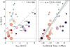 |
Fig. 7 Radial component of the relative cluster motions (vr) versus the tangential component (vtan) (left panel), and versus formation time (right panel), with e Lup as a reference point. Symbols and colours are as in Fig. 4. The dashed grey line in the left panel is a 1-to-1 line. The dashed dark grey line in the right panel shows a linear fit to data of 23 clusters, after removing the seven red-circled and the two dashed black-circled clusters. The solid light grey line at vr = 0 in both panels marks the transition from radial outward motion (> 0) to inward motion (< 0). |
5.3 Radial propagation speed of star formation
Looking at the relations in Figs. 4 and 5, we find that we can combine the resulting linear relations from the speed-time (dv/dt) and radial-motion-distance (dvr/dr) relations, to determine the radial propagation speed of star formation (dr/dt). In this case, we are ignoring that we first have the speed (v) and second only the radial component of the motions (vr). Then we can write
 (6)
(6)
When using instead the dvr/dt relation from Fig. 7 (right panel) we can compare the same quantities; we get
 (7)
(7)
However, in the latter case, the seven odd clusters are not included in the value of dvr/dt. Additionally, we directly plot the relative cluster distances versus time to get dr/dt, shown in Fig. 8. Again, we find that the seven odd clusters appear to be outliers, while the rest of the clusters follow roughly a linear relation. When ignoring the odd clusters, we get a relation of about 6.2pcMyr−1 (6.0 km s−1), similar to Eq. (7).
We find that the radial propagation speed of star formation (assuming isotropic expansion) roughly matches or is higher than the total, present-day velocity dispersion of the entire system with σ3D ~ (4 to 4.7) km/s. This implies that the system is dominated by expansion, rather than random motions, and that it was initially dynamically cold.
5.4 Discussing and comparing the cumulative trends
The visible steps seen in the cumulative size in Fig. 3 suggest structure in the chronological, spatial cluster arrangement, when considering their present-day XYZ positions. However, this measurement does not include orbital tracebacks, as is also outlined above (Sects. 3 and 4.1). In this work, we have refrained from including orbital tracebacks due to several limitations and assumptions that have to be made, and because it would go beyond the scope of this paper, while tracebacks will be addressed in future work. For instance, assumptions have to be made concerning the various literature-reported values for the Galactic potential or the solar parameters, and one also needs to consider possible internal gravitational effects. Additionally, when measuring the size with the here presented method (Appendix B.2), we would need to trace back the individual stars; however, the majority of the member stars have no RVs or too large velocity uncertainties, which makes it unfeasible to use the same method. If, instead, we were to use only the average cluster positions, this would also require additional assumptions (e.g., changing cluster volumes due to cluster expansion, nonsphericity). Finally, orbital tracebacks are sensitive to the initial conditions. While the cluster median positions and velocities are generally more robust than those of single stars, any uncertainties would still inflate the traceback errors for longer integration times.
We preliminarily tested the influence of the tracebacks on the cumulative size estimate to get an understanding of the ‘true’ evolution of the association’s size. For this, we used the clusters’ median XYZ and UVW as initial conditions to calculate orbital tracebacks (using galpy, MWPotential2014, an axisymmetric potential from Bovy 2015). This allowed us to use the trace-backed positions at each time step for the cumulative size instead of the present-day positions, while the individual cluster extents were ignored. We find that the region was more compact in the past, consistent with the general expansion we find in this paper. This preliminary backward integration demonstrates that the absolute size at a given lookback time decreases substantially, while this measurement is sensitive to the adopted dynamical model and uncertainties of the initial conditions (e.g., assumed acceleration history, Galactic potential, internal gravity, internal expansion, or individual cluster extent). Considering that the clusters have relative velocities of several kilometres per second, backward integration over 10-20 Myr leads to position shifts of order 50-150 pc. However, while the absolute scale of the trace-backed cumulative size is model-dependent and sensitive to uncertainties, its qualitative behaviour is largely governed by the relative spatial offsets between successively formed cluster groups. Backward integration compresses the overall structure but preserves the age-ordered, inside-out arrangement of clusters, because these offsets are coupled to the measured expansion pattern (Figs. 4-6). This test also shows that the given presentday cumulative size in Fig. 3 represents an upper limit to the true physical extent of Sco-Cen at earlier times.
On the other hand, the stepwise increases in cumulative size largely disappear when using the trace-back positions. Nevertheless, looking at both trends in Figs. 1 and 3, we see that the cumulative σ3D and present-day cumulative size are increasing similarly when ordered by decreasing cluster age, with similar jumps and plateaus. The cumulative σ3D could be interpreted as the evolution of velocity dispersion over time during the star formation history of Sco-Cen, since the velocity dispersion of the stars should not have changed significantly since their formation, considering the relevant timescales; the velocity dispersion is invariant under uniform translation and insensitive to expansion offsets between cluster centroids since it measures velocity scatter. However, as has been pointed out, the size is sensitive to spatial offsets; thus, the cumulative size in Fig. 3 only represents the present-day arrangement of clusters. Therefore, the two measurements are not strictly equivalent and cannot be compared at face value. Still, the similarities between the two trends are intriguing, and their parallel behaviour might be physically suggestive. It appears that Sco-Cen’s dynamical history might also be encoded in the present-day cluster arrangement within the region. Modelling is needed to test how, in regions with massive stars, feedback (e.g., acceleration of cloud parts before stars form) might influence the eventual cluster configuration of an OB association, to better understand if we can learn more about an association’s history via such diagrams.
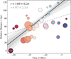 |
Fig. 8 Relative cluster distances versus formation time, with e Lup as a reference point. Symbols and colours as in Fig. 4. Two linear relations are fitted, once for all clusters (dashed light grey line) and once for 25 clusters (solid black line) after removing the seven red-circled clusters; see also Fig. 7. The shaded grey areas show the 1-2σ uncertainty ranges around the median slope when using 25 clusters. |
5.5 The importance of high-resolution age maps
Our work underscores the importance of identifying the substructure and age distribution within a stellar association. When populations within an association are mixed, which is often unavoidable when studying more distant regions, the observed velocity dispersion may be misconstrued. Even Sco-Cen, the closest OB association to Earth, was traditionally divided into only three subgroups with three different ages (see Appendix A.1). Thanks to Gaia, we now know that Sco-Cen comprises more than 30 individual stellar populations, each with distinct motions and ages, and with relatively low internal velocity dispersions per cluster.
Looking at earlier studies, Comeron et al. (1998) reported line-of-sight velocity dispersions of up to 60kms−1 for the Cygnus superbubble and up to 15kms−1 for the Canis Major OB1 association. They interpret these values as evidence for energetic expansion during the formation of these OB associations. Although this scenario is qualitatively consistent with our findings, we measure a significantly lower velocity dispersion for the entire Sco-Cen region, around 4-5kms−1. These relatively high velocity dispersions, reported by Comeron et al. (1998), could be real or could be due to various factors, such as the selection of RVs, instrumental limitations, or treatment of outliers and contamination. A likely contributor to the discrepancy is the presence of binary systems. In more distant clusters, the observed sample is typically dominated by massive stars, which are more likely to be multiples, even with careful selection, and thus introduce additional dispersion in the measured velocities.
Regardless of the differences of the final, total values of σ3D, we highlight in our work the importance of dissecting an association into its individual stellar clusters, with low velocity dispersions individually (of the order of 1-2kms−1) and with different ages. This allows us to produce high-resolution age maps and study the evolution of velocity dispersion in detail (Fig. 2). We conclude that the relatively high velocity dispersion of an OB association is the product of mixing stellar clusters within one region. Still, the discrepancy in the measured velocity dispersions in different literature needs more attention in future studies.
In conclusion, the presence of subpopulations and detailed age gradients found for the closest OB association to Earth should be considered when studying more distant regions or when modelling the evolution of OB associations. Our results, along with those of others (e.g. Kerr et al. 2021; Chen et al. 2020; Hunt & Reffert 2023), indicate that OB associations should not be treated as a single stellar population (e.g. Brown et al. 1997) or as simply a collection of a few subgroups (e.g. de Zeeuw et al. 1999), but rather as complex structures (e.g. Pecaut & Mamajek 2016; Wright & Mamajek 2018) composed of sequentially forming subpopulations (R23b; P25; MR25).
6 Summary and conclusions
This study presents the first reconstruction of the time evolution of stellar velocity dispersion in an OB association, using Sco-Cen as a case study. By combining high-precision Gaia DR3 astrometry with supplementary RV measurements, we analysed the kinematics of 32 stellar clusters spanning ages from about 3 to 21 Myr. We find that the stellar members of the whole Sco-Cen association yield a total, present-day 3D velocity dispersion of about 4-5 km s−1.
Moreover, we find a stepwise increase in the cumulative 3D velocity dispersion over time, together with a systematic insideout age sequence that is present in the 3D distribution of clusters in the Sco-Cen association. These patterns support a structured, sequential formation scenario, in which feedback from massive stars originating from older clusters likely shaped the formation and early kinematics of younger populations. The observed jumps in velocity dispersion align with known bursts of star formation (approximately separated by 5 Myr), indicating that Sco-Cen assembled in phases from spatially and kinematically distinct gas reservoirs.
The motions of the Sco-Cen clusters reveal a well-defined expansion pattern, with a present-day rate of approximately 1012 pc Myr−1, and a propagation speed of star formation of about 5-6kms−1. The expansion likely began 11-14 Myr ago, as is indicated by the outward motions, which are correlated with distance from the centre. The nearly isotropic velocity distribution suggests that internal dynamics and stellar feedback dominate over Galactic shear or differential rotation on the relevant timescales (∼20Myr) and spatial scales (∼200pc).
Our findings highlight the importance of high-resolution age maps and detailed kinematic substructure analysis in the study of OB associations. Simplistically treating these associations as single, homogeneous populations risks obscuring their complex formation pathways and underestimating their internal kinematic diversity. The sequential formation and expanding structure of Sco-Cen demonstrates the value of resolved, multi-epoch analyses for tracing the dynamical evolution and feedback processes in star-forming regions.
Data availability
Catalogues and data described in Appendix C are available at the CDS via https://cdsarc.cds.unistra.fr/viz-bin/cat/J/A+A/709/A181.
Acknowledgements
We thank the two referees for their constructive comments and feedback that improved the final version of this manuscript. We further thank Bruce Elmegreen and Jan Palous for valuable comments on our analysis. JG acknowledges funding from the European Union, the Central Bohemian Region, and the Czech Academy of Sciences, as part of the MERIT fellowship (MSCA-COFUND Horizon Europe, Grant agreement 101081195); the Collaborative Research Center 1601 (SFB 1601) funded by the Deutsche Forschungsgemeinschaft (DFG, 500700252); and the Austrian Research Promotion Agency (FFG, https://www.ffg.at/), project number 873708. SR acknowledges funding by the Federal Ministry of the Republic of Austria for Climate Action, Environment, Energy, Mobility, Innovation, and Technology (BMK, https://www.bmk.gv.at/) and FFG under project number FO999892674; SR performed this work as an SAO postdoctoral fellow and acknowledges the Smithsonian Institution for their support. Co-funded by the European Union (ERC, ISM-FLOW, 101055318). Views and opinions expressed are, however, those of the author(s) only and do not necessarily reflect those of the European Union or the European Research Council. Neither the European Union nor the granting authority can be held responsible for them. This work has made use of data from the European Space Agency (ESA) mission Gaia (https://www.cosmos.esa.int/gaia), processed by the Gaia Data Processing and Analysis Consortium (DPAC, https://www.cosmos.esa.int/web/gaia/dpac/consortium). Funding for the DPAC has been provided by national institutions, in particular, the institutions participating in the Gaia Multilateral Agreement. This work has made use of Python (https://www.python.org); Astropy (Astropy Collaboration 2013, 2022); NumPy (van der Walt et al. 2011); Matplotlib (Hunter 2007); SciPy (Virtanen et al. 2020); Galpy (Bovy 2015); TOPCAT (Taylor 2005); and the VizieR catalog access tool (Ochsenbein et al. 2000) and Aladin sky atlas (Bonnarel et al. 2000; Boch & Fernique 2014) operated at CDS, Strasbourg Observatory, France.
References
- Abdurro’uf, Accetta, K., Aerts, C., et al. 2022, ApJS, 259, 35 [NASA ADS] [CrossRef] [Google Scholar]
- Alves, J., Lombardi, M., & Lada, C. J. 2025, A&A, 697, A208 [NASA ADS] [CrossRef] [EDP Sciences] [Google Scholar]
- Astropy Collaboration (Robitaille, T. P., et al.) 2013, A&A, 558, A33 [NASA ADS] [CrossRef] [EDP Sciences] [Google Scholar]
- Astropy Collaboration (Price-Whelan, A. M., et al.) 2022, ApJ, 935, 167 [NASA ADS] [CrossRef] [Google Scholar]
- Bennett, M., & Bovy, J. 2019, MNRAS, 482, 1417 [NASA ADS] [CrossRef] [Google Scholar]
- Biazzo, K., Alcalá, J. M., Covino, E., et al. 2012, A&A, 547, A104 [NASA ADS] [CrossRef] [EDP Sciences] [Google Scholar]
- Blaauw, A. 1946, Publ. Kapteyn Astron. Lab. Groningen, 52, 1 [NASA ADS] [Google Scholar]
- Blaauw, A. 1964a, ARA&A, 2, 213 [Google Scholar]
- Blaauw, A. 1964b, in The Galaxy and the Magellanic Clouds, 20, ed. F. J. Kerr, 50 [Google Scholar]
- Boch, T., & Fernique, P. 2014, in Astronomical Society of the Pacific Conference Series, 485, Astronomical Data Analysis Software and Systems XXIII, eds. N. Manset, & P. Forshay, 277 [Google Scholar]
- Bonnarel, F., Fernique, P., Bienaymé, O., et al. 2000, A&AS, 143, 33 [Google Scholar]
- Bovy, J. 2015, ApJS, 216, 29 [NASA ADS] [CrossRef] [Google Scholar]
- Breitschwerdt, D., Feige, J., Schulreich, M. M., et al. 2016, Nature, 532, 73 [NASA ADS] [CrossRef] [Google Scholar]
- Bressan, A., Marigo, P., Girardi, L., et al. 2012, MNRAS, 427, 127 [NASA ADS] [CrossRef] [Google Scholar]
- Brown, A. G. A., Dekker, G., & de Zeeuw, P. T. 1997, MNRAS, 285, 479 [NASA ADS] [CrossRef] [Google Scholar]
- Buder, S., Sharma, S., Kos, J., et al. 2021, MNRAS, 506, 150 [NASA ADS] [CrossRef] [Google Scholar]
- Buder, S., Kos, J., Wang, E. X., et al. 2024, arXiv e-prints [arXiv:2409.19858] [Google Scholar]
- Castro-Ginard, A., Penoyre, Z., Casey, A. R., et al. 2024, A&A, 688, A1 [NASA ADS] [CrossRef] [EDP Sciences] [Google Scholar]
- Chen, C. H., Mamajek, E. E., Bitner, M. A., et al. 2011, ApJ, 738, 122 [NASA ADS] [CrossRef] [Google Scholar]
- Chen, B., D’Onghia, E., Alves, J., & Adamo, A. 2020, A&A, 643, A114 [NASA ADS] [CrossRef] [EDP Sciences] [Google Scholar]
- Comeron, F., Torra, J., & Gomez, A. E. 1998, A&A, 330, 975 [NASA ADS] [Google Scholar]
- Dahm, S. E., Slesnick, C. L., & White, R. J. 2012, ApJ, 745, 56 [NASA ADS] [CrossRef] [Google Scholar]
- Dale, J. E., Haworth, T. J., & Bressert, E. 2015a, MNRAS, 450, 1199 [NASA ADS] [CrossRef] [Google Scholar]
- Daniel, W. 1990, Applied Nonparametric Statistics, Duxbury Advanced Series in Statistics and Decision Sciences (PWS-KENT Pub.) [Google Scholar]
- de Avillez, M. A., & Breitschwerdt, D. 2005, A&A, 436, 585 [NASA ADS] [CrossRef] [EDP Sciences] [Google Scholar]
- de la Fuente Marcos, R., & de la Fuente Marcos, C. 2008, ApJ, 672, 342 [Google Scholar]
- De Silva, G. M., Freeman, K. C., Bland-Hawthorn, J., et al. 2015, MNRAS, 449, 2604 [NASA ADS] [CrossRef] [Google Scholar]
- de Zeeuw, P. T., Hoogerwerf, R., de Bruijne, J. H. J., Brown, A. G. A., & Blaauw, A. 1999, AJ, 117, 354 [Google Scholar]
- Dijkstra, E. W. 1959, Numer. Math., 1, 269 [Google Scholar]
- Edenhofer, G., Zucker, C., Frank, P., et al. 2024a, A&A, 685, A82 [NASA ADS] [CrossRef] [EDP Sciences] [Google Scholar]
- Edenhofer, G., Alves, J., Zucker, C., Posch, L., & Enßlin, T. A. 2024b, A&A, 687, L9 [NASA ADS] [CrossRef] [EDP Sciences] [Google Scholar]
- Elmegreen, B. G., & Lada, C. J. 1977, ApJ, 214, 725 [Google Scholar]
- Fang, M., Pascucci, I., Edwards, S., et al. 2023, ApJ, 945, 112 [NASA ADS] [CrossRef] [Google Scholar]
- Fuchs, B., Breitschwerdt, D., de Avillez, M. A., Dettbarn, C., & Flynn, C. 2006, MNRAS, 373, 993 [NASA ADS] [CrossRef] [Google Scholar]
- Gaczkowski, B., Roccatagliata, V., Flaischlen, S., et al. 2017, A&A, 608, A102 [NASA ADS] [CrossRef] [EDP Sciences] [Google Scholar]
- Gagné, J., Roy-Loubier, O., Faherty, J. K., Doyon, R., & Malo, L. 2018a, ApJ, 860, 43 [Google Scholar]
- Gaia Collaboration (Brown, A. G. A., et al.) 2016, A&A, 595, A2 [NASA ADS] [CrossRef] [EDP Sciences] [Google Scholar]
- Gaia Collaboration (Vallenari, A., et al.) 2023, A&A, 674, A1 [NASA ADS] [CrossRef] [EDP Sciences] [Google Scholar]
- Galli, P. A. B., Bertout, C., Teixeira, R., & Ducourant, C. 2013, A&A, 558, A77 [NASA ADS] [CrossRef] [EDP Sciences] [Google Scholar]
- Gilmore, G., Randich, S., Asplund, M., et al. 2012, Messenger, 147, 25 [Google Scholar]
- Gontcharov, G. A. 2006, Astron. Lett., 32, 759 [Google Scholar]
- Großschedl, J. E., Alves, J., Meingast, S., & Herbst-Kiss, G. 2021, A&A, 647, A91 [NASA ADS] [CrossRef] [EDP Sciences] [Google Scholar]
- Guenther, E. W., Esposito, M., Mundt, R., et al. 2007, A&A, 467, 1147 [CrossRef] [EDP Sciences] [Google Scholar]
- Hunt, E. L., & Reffert, S. 2023, A&A, 673, A114 [NASA ADS] [CrossRef] [EDP Sciences] [Google Scholar]
- Hunter, J. D. 2007, Comput. Sci. Eng., 9, 90 [NASA ADS] [CrossRef] [Google Scholar]
- Hutschenreuter, S., Alves, J., Posch, L., et al. 2026, A&A, 705, A108 [NASA ADS] [CrossRef] [EDP Sciences] [Google Scholar]
- Jackson, R. J., Jeffries, R. D., Wright, N. J., et al. 2022, MNRAS, 509, 1664 [Google Scholar]
- James, D. J., Melo, C., Santos, N. C., & Bouvier, J. 2006, A&A, 446, 971 [NASA ADS] [CrossRef] [EDP Sciences] [Google Scholar]
- Jilinski, E., Daflon, S., Cunha, K., & de La Reza, R. 2006, A&A, 448, 1001 [NASA ADS] [CrossRef] [EDP Sciences] [Google Scholar]
- Joergens, V., & Guenther, E. 2001, A&A, 379, L9 [NASA ADS] [CrossRef] [EDP Sciences] [Google Scholar]
- Kamaya, H. 2004, AJ, 128, 761 [Google Scholar]
- Katz, D., Sartoretti, P., Guerrier, A., et al. 2023, A&A, 674, A5 [NASA ADS] [CrossRef] [EDP Sciences] [Google Scholar]
- Kerr, R. M. P., Rizzuto, A. C., Kraus, A. L., & Offner, S. S. R. 2021, ApJ, 917, 23 [NASA ADS] [CrossRef] [Google Scholar]
- Kollmeier, J. A., Zasowski, G., Rix, H.-W., et al. 2017, arXiv e-prints [arXiv:1711.03234] [Google Scholar]
- Kollmeier, J., Anderson, S. F., Blanc, G. A., et al. 2019, in Bulletin of the American Astronomical Society, 51, 274 [Google Scholar]
- Kollmeier, J. A., Rix, H.-W., Aerts, C., et al. 2026, AJ, 171, 52 [Google Scholar]
- Kos, J., Bland-Hawthorn, J., Asplund, M., et al. 2019, A&A, 631, A166 [NASA ADS] [CrossRef] [EDP Sciences] [Google Scholar]
- Krause, M. G. H., Burkert, A., Diehl, R., et al. 2018, A&A, 619, A120 [NASA ADS] [CrossRef] [EDP Sciences] [Google Scholar]
- Kroupa, P. 1995, MNRAS, 277, 1522 [NASA ADS] [CrossRef] [Google Scholar]
- Kroupa, P. 2008, in The Cambridge N-Body Lectures, 760, eds. S. J. Aarseth, C. A. Tout, & R. A. Mardling, (Springer Dordrecht), 181 [Google Scholar]
- Kuhn, M. A., Hillenbrand, L. A., Sills, A., Feigelson, E. D., & Getman, K. V. 2019, ApJ, 870, 32 [CrossRef] [Google Scholar]
- Kunder, A., Kordopatis, G., Steinmetz, M., et al. 2017, AJ, 153, 75 [Google Scholar]
- Lada, C. J., & Lada, E. A. 2003, ARA&A, 41, 57 [Google Scholar]
- Lada, C. J., Margulis, M., & Dearborn, D. 1984, ApJ, 285, 141 [NASA ADS] [CrossRef] [Google Scholar]
- Lindegren, L., Klioner, S. A., Hernández, J., et al. 2021, A&A, 649, A2 [EDP Sciences] [Google Scholar]
- Luhman, K. L. 2023, AJ, 165, 269 [NASA ADS] [CrossRef] [Google Scholar]
- Lynga, G., & Palous, J. 1987, A&A, 188, 35 [NASA ADS] [Google Scholar]
- Mamajek, E. E., & Feigelson, E. D. 2001, in Astronomical Society of the Pacific Conference Series, 244, Young Stars Near Earth: Progress and Prospects, eds. R. Jayawardhana, & T. Greene, 104 [Google Scholar]
- Majewski, S. R., Schiavon, R. P., Frinchaboy, P. M., et al. 2017, AJ, 154, 94 [NASA ADS] [CrossRef] [Google Scholar]
- Mészáros, S., Jofré, P., Johnson, J. A., et al. 2025, AJ, 170, 96 [Google Scholar]
- Miret-Roig, N., Galli, P. A. B., Olivares, J., et al. 2022, A&A, 667, A163 [NASA ADS] [CrossRef] [EDP Sciences] [Google Scholar]
- Miret-Roig, N., Alves, J., Ratzenböck, S., et al. 2025, A&A, 694, A60 [NASA ADS] [CrossRef] [EDP Sciences] [Google Scholar]
- Murphy, S. J., Lawson, W. A., & Bessell, M. S. 2013, MNRAS, 435, 1325 [Google Scholar]
- Neuhäuser, R., Gießler, F., & Hambaryan, V. V. 2020, MNRAS, 498, 899 [CrossRef] [Google Scholar]
- Nguyen, D. C., Brandeker, A., van Kerkwijk, M. H., & Jayawardhana, R. 2012, ApJ, 745, 119 [Google Scholar]
- Ochsenbein, F., Bauer, P., & Marcout, J. 2000, A&AS, 143, 23 [Google Scholar]
- Pearson, K. 1895, Proc. Roy. Soc. Lond. Ser. I, 58, 240 [NASA ADS] [CrossRef] [Google Scholar]
- Pecaut, M. J., & Mamajek, E. E. 2016, MNRAS, 461, 794 [Google Scholar]
- Poleski, R. 2013, arXiv e-prints [arXiv:1306.2945] [Google Scholar]
- Posch, L., Miret-Roig, N., Alves, J., et al. 2023, A&A, 679, L10 [NASA ADS] [CrossRef] [EDP Sciences] [Google Scholar]
- Posch, L., Alves, J., Miret-Roig, N., et al. 2025, A&A, 693, A175 [NASA ADS] [CrossRef] [EDP Sciences] [Google Scholar]
- Preibisch, T., & Zinnecker, H. 1999, AJ, 117, 2381 [NASA ADS] [CrossRef] [Google Scholar]
- Preibisch, T., & Mamajek, E. 2008, in Handbook of Star Forming Regions, Volume II, 5, ed. B. Reipurth (Astronomical Society of the Pacific), 235 [Google Scholar]
- Ratzenböck, S., Großschedl, J. E., Möller, T., et al. 2023a, A&A, 677, A59 [NASA ADS] [CrossRef] [EDP Sciences] [Google Scholar]
- Ratzenböck, S., Großschedl, J. E., Alves, J., et al. 2023b, A&A, 678, A71 [NASA ADS] [CrossRef] [EDP Sciences] [Google Scholar]
- Sacco, G. G., Spina, L., Randich, S., et al. 2017, A&A, 601, A97 [NASA ADS] [CrossRef] [EDP Sciences] [Google Scholar]
- Santana, F. A., Beaton, R. L., Covey, K. R., et al. 2021, AJ, 162, 303 [NASA ADS] [CrossRef] [Google Scholar]
- Schönrich, R., Binney, J., & Dehnen, W. 2010, MNRAS, 403, 1829 [NASA ADS] [CrossRef] [Google Scholar]
- Slesnick, C. L., Hillenbrand, L. A., & Carpenter, J. M. 2008, ApJ, 688, 377 [NASA ADS] [CrossRef] [Google Scholar]
- Spearman, C. 1904, Am. J. Psychol., 15, 72 [Google Scholar]
- Squicciarini, V., Gratton, R., Bonavita, M., & Mesa, D. 2021, MNRAS, 507, 1381 [NASA ADS] [CrossRef] [Google Scholar]
- Steinmetz, M., Matijevic, G., Enke, H., et al. 2020a, AJ, 160, 82 [NASA ADS] [CrossRef] [Google Scholar]
- Swiggum, C., Alves, J., Benjamin, R., et al. 2024, Nature, 631, 49 [NASA ADS] [CrossRef] [Google Scholar]
- Swiggum, C., Alves, J., & D’Onghia, E. 2025, A&A, 699, L5 [NASA ADS] [CrossRef] [EDP Sciences] [Google Scholar]
- Taylor, M. B. 2005, in Astronomical Society of the Pacific Conference Series, 347, Astronomical Data Analysis Software and Systems XIV, eds. P. Shopbell, M. Britton, & R. Ebert, 29 [Google Scholar]
- Torres, C. A. O., Quast, G. R., da Silva, L., et al. 2006, A&A, 460, 695 [NASA ADS] [CrossRef] [EDP Sciences] [Google Scholar]
- Tsantaki, M., Pancino, E., Marrese, P., et al. 2022, A&A, 659, A95 [NASA ADS] [CrossRef] [EDP Sciences] [Google Scholar]
- van der Walt, S., Colbert, S. C., & Varoquaux, G. 2011, Comput. Sci. Eng., 13, 22 [Google Scholar]
- Virtanen, P., Gommers, R., Oliphant, T. E., et al. 2020, Nat. Methods, 17, 261 [Google Scholar]
- Wichmann, R., Covino, E., Alcalá, J. M., et al. 1999, MNRAS, 307, 909 [Google Scholar]
- Wright, N. J., & Mamajek, E. E. 2018, MNRAS, 476, 381 [Google Scholar]
- Wright, N. J., Kounkel, M., Zari, E., Goodwin, S., & Jeffries, R. D. 2023, in Astronomical Society of the Pacific Conference Series, 534, Astronomical Society of the Pacific Conference Series, eds. S. Inutsuka, Y. Aikawa, T. Muto, K. Tomida, & M. Tamura, 129 [Google Scholar]
We use the term ‘cluster’ in a statistical sense, as in R23a.
As in our quality criteria (Appendix A.4); chosen to ensure that also sparse clusters contain several stars with measured RVs.
We shall discuss the individual clusters’ velocity dispersions in a future work, since this requires a more careful selection of RVs and ideally a higher quantity of high-quality RVs. See also the caveats outlined in Appendix A.3.
The youngest period of enhanced star formation is less pronounced in our work, since we excluded the two, young Chamaeleon clusters, which are part of R23b.
Three clusters are likely unrelated: Norma-North, Oph-SE, and Oph-NF (see R23b).
astraAllStarASPCAP-O.6.0.fits from https://dr19.sdss.org/sas/dr19/spectro/astra/0.6.0/summary/.
Appendix A Used data and parameters
A.1 The Sco-Cen cluster sample
As in R23b, we considered only 34 out of the total 37 SigMA selected clusters from R23a as probable members of the Sco-Cen association5. We initially included the three removed clusters (Oph-Southeast, Oph-NorthFar, and Norma-North) in our analysis, and we can confirm that these are unrelated, since they show significantly different kinematics when compared to the rest of the Sco-Cen clusters. The 34 clusters contain a total of 12,972 stellar members. Each cluster was assigned to a traditional region (TR), as defined in 2D projection. The TRs include the classical Blaauw (1946) regions Upper-Scorpius (US), Upper Centaurus Lupus (UCL), and Lower Centaurus Crux (LCC), which have often been treated as the three stellar sub-groups of Sco-Cen (e.g. de Zeeuw et al. 1999; Mamajek & Feigelson 2001; Preibisch & Mamajek 2008). R23a further identified and included clusters toward Pipe, Corona Australis (CrA), and Chamaeleon (Cham), and to the Galactic north-east (NE) of Sco-Cen. The two clusters in the TW Hydrae association (TWA-a, TWA-b) were added to Sco-Cen by MR25, while stellar members were previously reported in Gagné et al. (2018a) or Luhman (2023). With this, there are 36 clusters in Sco-Cen contain a total of 13,011 stellar members.
In our analysis, we did not include the Chamaeleon clusters (Cham-I, Cham-II, Centaurus-Far), since these are connected to a background structure, as discussed in Edenhofer et al. (2024b). The authors identified a C-like structure in a 3D dust map (Edenhofer et al. 2024a), named ‘The C’. The shell-like structure was likely created by a supernova, creating a rim that contains the Chameleon, Musca, and Coalsack clouds, located at the back of the main Sco-Cen complex. The history of this structure is likely connected to Sco-Cen, where remaining gas was possibly influenced by massive stellar feedback originating from the OB association. Nevertheless, we removed the clusters that are associated with ‘The C’ structure from our current analysis, since the relative motions show peculiarities compared to the rest of the Sco-Cen clusters, and they are also located slightly detached from the main body of Sco-Cen. Moreover, we did not include the cluster μ Sco in our analysis, since it has poor RV statistics; only two stellar members passed the RV quality criteria (Appendix A.4), which additionally showed a large dispersion in RV space.
We combined the SigMA Sco-Cen sample with the TWA sample (66 stellar members). We found that 27 sources are in common, which are candidate members of σ Cen, a cluster which is connected to TWA in a cluster chain. The overlapping sources have low statistical stability for σ Cen, as given by the SigMA algorithm, and they are scattered suspiciously in front of the cluster along the line-of-sight, which makes it more likely that these sources belong to TWA (see also MR25). Hence, these 27 sources are assigned to TWA in this paper. TWA was tentatively split into two clusters in MR25, named TWA-a and TWA-b, containing 44 and 22 stellar members, respectively.
Consequently, we analysed 32 Sco-Cen clusters in this paper that contain a total of 12,612 stellar members, with 12,546 retrieved from the 30 SigMA Sco-Cen clusters (R23a) and 66 from the two TWA clusters (MR25). An overview of all 36 Sco-Cen clusters is given in Table A.2, listing the cluster names, ages, and number statistics, including the four excluded clusters.
A.2 Parameters and parameter transformations
We used the astrometric parameters from Gaia DR3 and supplementary RV data (see Appendix A.3):
α, δ (deg): Right ascension and Declination
l, b (deg): Galactic longitude and latitude
w (mas): parallax
d (pc): distance (1000/ϖcorr)
μα, μδ (mas yr−1): proper motions along α and δ (for simplicity we denote here μα cos(δ) as μα)
μl, μb (mas yr−1): proper motions along l and b (for simplicity we denote here μl cos(b) as μl)
vRV (kms−1): Heliocentric RV (line-of-sight motion relative to the Sun, determined from stellar spectra)
We corrected the parallaxes (ϖcorr) for the parallax bias identified in Lindegren et al. (2021), by subtracting the zero-point correction factor f_zpt (python package zero_point)6. In this work, we used the inverse of the corrected parallax as a distance estimate, which is reasonable for targets within about 200 pc from the Sun and for sources with low uncertainties (see R23a).
The velocities were corrected for the standard solar motion (Schönrich et al. 2010), hence transformed to velocities relative to the LSR with the help of astropy.coordinates (Astropy Collaboration 2022). They are given as μα,lsr, μδ,lsr, μl,lsr, μb,lsr (mas/yr) and vRV,lsr (km/s). The transformation from μx to μx,lsr can alternatively be achieved by the transformations outlined in Poleski (2013). The tangential velocities (vα, vδ, vl, vb, or vα,lsr, vδ,lsr, vl,lsr, vb,lsr) were derived from proper motions and parallaxes as follows:
 (A.1)
(A.1)
The proper motion can be entered heliocentric or LSR-corrected in the above formula, while the latter results in tangential velocities in the LSR frame. XYZ are the Heliocentric Galactic Cartesian co-ordinates in parsec (pc):
 (A.2)
(A.2)
Here X is positive toward the Galactic centre, Y is positive in the direction of Galactic rotation, and Z is positive toward the Galactic North Pole. The corresponding Heliocentric Galactic Cartesian velocities in the directions of XYZ are given as UVW (in km s−1):
 (A.3)
(A.3)
Substituting the given velocities with vRV,lsr, vl,lsr, and vb,lsr gives the Cartesian velocities relative to the LSR, denoted as ULSR, VLSR, and WLSR (kms−1). Alternatively, UVWLSR could be calculated from UVW by adding the values of the standard solar motion from Schönrich et al. (2010). In our analysis, one can use both the Heliocentric or LSR corrected Galactic Cartesian velocities, since it does not make a difference when investigating relative motions within a region.
To get uncertainties for the derived parameters, we used a Monte Carlo approach. We sampled from the various parameters by randomly drawing from Gaussians, using the measurements and their uncertainties as the mean and standard deviation. For instance, to get the uncertainties of the tangential velocities, we used Eq. (A.1), and we sampled over the parallaxes and proper motions using their uncertainties as the standard deviation of the Gaussian. We then used the median and standard deviation as the derived parameters and their uncertainties.
A.3 The radial velocity surveys
Table A.1 lists 22 RV surveys or literature studies that were combined in this work to get more complete 6D phase space information per cluster. The RV surveys were combined with the Gaia DR3 Sco-Cen catalogue (13 011 sources) by using the source IDs or sky cross-matches. A Gaia source_id match was possible for catalogues that contain information on Gaia, 2MASS, or HIP IDs, which can be matched within the Gaia archive (see also Appendix A in R23a). For other catalogues, we used a 1" cross-match radius, using the closest match.
The list in Table A.1 includes several well-known large-scale surveys and also smaller-scale spectroscopic studies. This created a heterogeneous RV sample, observed with different instruments at different resolutions, and processed with different pipelines. Hence, we are dealing with variable data coverage and possible systematic differences between the RV surveys. Moreover, the measurement uncertainties could have additional systematics and might have been estimated differently, further complicating a comparison at face value. One way forward could be to use an already homogenised catalogue, such as the Survey of Surveys (SoS) by Tsantaki et al. (2022), which is a compilation of six spectroscopic surveys (Gaia DR2, APOGEEDR16, GALAHDR2, Gaia-ESODR3, LAMOSTDR5, and RAVEDR6). However, most of the data releases (DR) of the included surveys have already been superseded by more recent releases. Hence, we decided to use the most recent DRs and other original literature data, which were not used by SoS.
Small systematic variations between surveys are not highly critical when averaging the motions per cluster to get each cluster’s median or mean motion, while for the calculation of the velocity dispersion, we aimed at higher quality. Hence, we applied quality criteria, outlined in Appendix A.4, and we compared the individually measured RVs to each other to identify possible systematic shifts between the surveys (for this, we matched the full external catalogues with Gaia DR3). Binaries could also cause discrepancies between measurements from different surveys; however, we would not expect a systematic shift in one direction between two surveys to be caused by binaries. We used Gaia DR3 RVs as zero-point, since this is the largest survey in our list, covering the whole sky; hence, we were able to compare it to the full available catalogues of the other surveys. We only identified significant global shifts in four cases: SDSS, GALAH, RAVE, and PCRV. For the rest of the surveys, we either did not find a significant shift or there were not enough sources in common to identify a clear trend. The average shifts are given in Table A.1 as ∆RV. We did not correct for these shifts, since we did not test for dependencies (relative to Teff, log g, or metallicity; see e.g. Tsantaki et al. 2022), which would have gone beyond the scope of this paper. To account for this additional uncertainty, we added the shift quadratically to the measurement uncertainties of these four surveys. Concerning the measurement uncertainties in general, we did not consider any systematics between the surveys, and we used the surveys’ reported RV uncertainties (eRV) for simplicity. We corrected the RV errors in the four mentioned cases as follows,  , and we used these values in the quality criteria below.
In the following, we give some details concerning RVs from the recently released SDSS DR19, which are part of the Milky Way Mapper (MWM) program, while we used observations from the APOGEE instruments. We used the MWM/Astra/ASPCAP catalogue7, which contains APOGEE RVs from SDSS-IV DR17 and SDSS-V DR19 (Kollmeier et al. 2026). The column ‘release’ specifies if a source originates from the earlier (dr17) or the more recent (sdss5) data release. SDSS also provides a scatter parameter (std_v_rad) for sources observed more than once within the MWM survey, which can be used to remove potential multiple stellar systems. We recomputed the SDSS RV uncertainties as follows:  . Using the corrected RV errors, sources with larger scatter (potential binary candidates) get automatically removed when applying the error cuts as outlined in the next section. Sources without the scatter information, which were observed only once within SDSS, lack this information, and their errors might be underestimated. At this stage, we can not know about any additional scatter for such sources, if only observed by one survey. Some sources are observed by multiple RV surveys that are listed in Table A.1, and we outlined the scatter estimate for such sources in the next section.
A.4 Quality criteria
First, we used the stability criterion per stellar cluster member that was provided in the SigMA catalogue (R23a). This criterion indicates how often individual sources appear throughout the ensemble of clustering solutions per cluster, denoted as stability in the range from 0-100%; hence, sources with low stability are less reliable cluster members. The maximum stability per cluster is variable, while generally higher for richer clusters, since they have been more often retained by SigMA. Hence, we applied a variable stability cut per cluster, which is set as follows. R23a found that stars in more ‘stable’ clusters (generally the richer and more massive ones) have generally higher stability values (>80%). R23a suggested that a cut at about stability > 11% would be a reasonable discriminator for such clusters to select more reliable stellar cluster members. We decided to create a variable stability cut to account for the fact that the stability values of stars within sparser clusters are generally lower. First, we calculated the median stability per cluster, and then we used 10% of the median as the threshold, which gives less conservative values than the suggested 11%. The resulting value is used as the individual stability threshold per cluster: stab_lim = median_stability (per cluster) ∙ 0.1. This value is listed in Table A.2 (Col. 5). We then only kept stars with stability > stab_lim. This procedure gave us lower stability thresholds than 11% for all clusters, which ensured that we only removed the most obvious outliers, which is in particular critical for the less prominent clusters. This variable stability cut was applied both to the positional and the velocity data, while the latter required additional quality checks for the RV data, as follows.
The sample size of the 3D velocity data (UVW) strongly depends on the available RV data (Table A.1). We found that about 50% of the sources (6540/13 011) have been targeted by at least one RV survey. Considering these sources, approximately 34% have been targeted by more than one survey (2205/6540).
Data references for radial velocities.
This sample can be used to identify binary candidates. Additionally, we investigated the Gaia DR3 RUWE parameter (Castro-Ginard et al. 2024) that indicates if a source is a probable binary or multiple stellar system, further discussed in Appendix B.1.
To obtain a clean sample of RVs per cluster while retaining a significant number of sources, we applied the following quality criteria. In a first step, we retained only sources with low RV uncertainties, using a cut at eRV < 3.1 kms−1 (using eRV,corr < 3.1 km s−1 when a correction was applied). We decided on a relatively non-conservative cut to ensure that clusters with few RV measurements contain significant numbers of sources with RV information.
For sources with multiple observations from different surveys, we first calculated the weighted mean and weighted standard deviation as follows:
 (A.4)
(A.4)
where  are the weights. For our analysis, if a source was observed multiple times, we used the RV measurement from the survey with the lowest error (named vRV,best). The weighted mean and standard deviation are used to test for significant deviations between the surveys, to remove potential binary or multiple candidates (similar to the scatter in SDSS). We kept sources with
  and eRV,w < 3.1 kms−1. We decided for this cut to be comparable to the used RV error cut introduced above.
After these applied cuts, there are still some RVs per cluster that are clearly scattered beyond the clusters’ median RVs. Significant deviations in the motions of single stars from the bulk motion of the parent cluster could have several reasons, such as unresolved binaries, mismatches, or contamination from unrelated stellar populations or field stars. To clean the RV sample per cluster, we excluded potential contaminants or outliers first via a global outlier cut and second via sigma clipping. We used the LSR corrected RVs (vRV,lsr); they show less scatter, since artificial trends are removed that appear when using the heliocentric RVs. First, when considering the RV distribution of the whole Sco-Cen association, we found that sources scattered beyond  are general outliers, and we globally removed sources beyond these boundaries. Next, we removed outliers with significant deviations from the bulk motion of each cluster by applying sigma clipping at 3σ around each cluster’s median (vRV,lsr). In most cases, this additional step removed only a few outliers or none.
Overview of 36 stellar clusters toward Sco-Cen from R23a (SigMA selected clusters) and MR25 (TWA clusters), including RV data statistics, sorted by cluster age. An extended online version of this table is available on Vizier, which also contains further cluster properties, such as average positions and motions, as shown in the column overview in Table C.2.
Finally, the combined quality criteria, including the stability cut, error cuts, removal of binary candidates, and sigma-clipping, leave 3240 (25%) sources out of 13,011. The individual numbers and fractions per cluster are given in Table A.2. We compared the weighted mean with the finally selected best RVs per source (when observed multiple times) after applying the mentioned quality criteria. We did not find a significant deviation for the majority of these sources:  km/s, underlining the robustness of these selected RVs.
Appendix B Detailed method descriptions
B.1 Calculating the cumulative velocity dispersion
Here, we give more details on the construction of Fig. 1, which shows the change of the cumulative 3D velocity dispersion with cluster age or formation time. The cumulative σ3D was calculated chronologically by incorporating the stellar members of the clusters that lie within a certain age threshold. In more detail, we started to calculate σ3D by using the stellar members of the oldest cluster, e Lup, and then added chronologically at each step the stars of the next youngest cluster, until we reached the final step that contains all stars in Sco-Cen, from old to young. At each step, we calculated the total velocity dispersion of the stellar members that formed before the time threshold as given on the x-axis of Fig. 1, which resulted in the cumulative velocity dispersion over a time span of about 20 Myr.
To account for the different sample sizes of each cluster -several clusters contain only a handful of RVs (see Table A.2) - we used at each time-step a random subsample of 20 sources per cluster. This sub-sampling was done to avoid the dispersion estimations being dominated by the sample size, which would naturally give more weight to the more massive clusters or the clusters that contain a higher number of observed RVs. The relatively low number of 20 was chosen to account for the fact that several clusters have very low number statistics, especially when requiring good RV data quality. If a cluster had fewer than 20 members, then we randomly sampled 20 data points with replacement. This up-sampling concerned nine out of the 32 clusters. We repeated this procedure 1000 times, and each time randomly drew another 20 stars from each cluster, which delivered a median and uncertainty for σ3D at each time step, as plotted in Fig. 1. By iteratively adding random sub-samples of stellar members of each cluster one after another, we obtained an increase in velocity dispersion, until the total velocity dispersion of the whole association was reached with 4.64±0.04 km s−1 (see also Table B.1).
As outlined in Sect. 4, we compared the total σ3D from the sub-sampling approach to the total σ3D when all available stellar members of the 32 clusters in Sco-Cen are used for its calculation. Hence, we used all stars in the 32 clusters that pass our quality criteria (i.e., 3123 out of 12612), instead of 20 subsamples from each cluster (the latter resulted in a sample of only 640 stars when the final time-step is reached). We bootstrapped over the 3123 available sources with replacement 10 000 times. The mean of the bootstrap samples resulted in a 3D velocity dispersion of 3.97±0.03 km s−1, which is about 0.7 km/s lower than the final value of the cumulative σ3D. This difference might be caused by the undersampling of the velocity space when only using sub-samples, which might also increase the importance of individual measurement errors, which could inflate the final σ3D. At the same time, the total velocity dispersion using all available stars might be dominated by the most massive clusters, which contain overall more stars with valid RV measurements.
To test the influence of RV measurement errors, we recalculated the cumulative σ3D using two alternative data samples. First, we applied an additional RV error cut at eRV < 1 km s−1 (and eRVw < 1 km s−1 if a source was observed by more than one survey). In some cases, this reduced the number of stellar members per cluster significantly; for 13 clusters, there were then fewer than 20 members available, so their numbers had to be up-sampled. Nevertheless, when comparing the resulting trend to the original one form Fig. 1, we found that the cumulative velocity dispersion increased similarly over time, while there was only a shift to overall lower values, on average about −0.2 kms−1 (see Fig. B.1, blue curve), and the total σ3D results in 4.46±0.03kms−1.
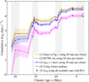 |
Fig. B.1 Influence of measurement errors or binaries on the cumulative σ3D. (1) The upper orange curve is the fiducial one from Fig. 1. (2) The dashed black curve shows the cumul. σ3D when applying a cut on the Gaia RUWE parameter, to test the influence of binaries. (3) The middle blue curve shows the cumul. σ3D when applying an additional error cut at eRV ≤ 1 km s−1 on the stellar members of each cluster. (4) The magenta curve shows the cumul. σ3D when using the cluster medians. (5) The black cross marks the total σ3D as calculated from all stars in Sco-Cen with valid RV measurements. The error bars (shaded regions) show the 95% interquartile ranges (2σ). |
Results of the total σ3D of the whole Sco-Cen association when using the different, mentioned data samples.
Second, we calculated the cumulative velocity dispersion by using only the median UVW values of the clusters. With this approach, we removed any internal velocity scatter of each cluster, and we only focused on the more robust cluster velocities; so we got a measure of the lower limit of σ3D. We sampled from cluster median UVW velocities and their uncertainties (assuming Gaussian errors) to get a measure of uncertainty for the clusters’ cumulative σ3D. Naturally, this approach results in lownumber statistics, especially for the first few time-steps (at the start, only one velocity is used, from e Lup, hence, it is zero). Nevertheless, we found that the shape of the curve is similar, as highlighted in Fig. B.1 (magenta curve), with an average shift of about −0.5 to −0.6 km s−1. The total 3D velocity dispersion of all 32 cluster medians results in 4.13±0.06 km s−1.
Finally, we tested the potential influence of unresolved binaries or multiples. We used Gaia’s re-normalised unit weight error (RUWE), and a variable limit (ruwe_lim) as outlined in Castro-Ginard et al. (2024, see their Appendix A). The suggested ruwe_lim mainly depends on crowding at the location of a star in the field of view of Gaia. We repeated the calculation of the cumulative σ3D by additionally requiring RUWE <ruwe_lim and compared it to the cumulative σ3D from Fig. 1. We find that the RUWE cut does not make a significant difference (Fig. B.1, dashed black line). Overall, we only find small deviations of about 0.01-0.03 km s−1 around the original trend. The total σ3D when using the RUWE cut is then 4.62±0.05 km s−1. We conclude that the influence of unresolved binaries is negligible concerning our selected UVW sample and that the influence of RV measurement errors is dominating any potential shifts of σ3D.
Considering these different tests, we conclude that the present-day velocity dispersion of Sco-Cen is between 4.04.7 km s−1 (see the overview in Table B.1). The measurement errors appear to influence the magnitude of the cumulative σ3D, while the increasing trend, with the visible jumps and plateaus in between, appears to be unaffected and stays essentially the same.
B.2 Calculating the cumulative size of the region
To estimate the cumulative size (S in parsecs; see Fig. 3) of Sco-Cen, we estimated the change of the extent of the region when ordering the stars by the ages of their parent clusters, starting with the oldest cluster, similar to the cumulative σ3D. We like to note that orbital tracebacks of the star and cluster positions have not been considered in this work, which will be part of future work. To calculate the size of a given assembly of stars in 3D, we determined the largest distance between any two sources at this step. Since Euclidean distances ignore the shape of Sco-Cen, we use a graph constructed from individual members (as nodes) to approximate the manifold of the association. We constructed the graph via a k-neighbours graph in positional (XYZ) space and used Dijkstra’s algorithm to compute shortest paths between any two sources in the graph (Dijkstra 1959). At each age step, we computed the maximum distance for all possible shortest paths between members of respective subgroups. We used the Python packages: sklearn.neighbors.kneighbors_graph, networkx, nx.single_source_dijkstra_path_length.
This was done cumulatively, by starting with the stellar members from the oldest cluster, and adding at each step stellar members of the next youngest cluster, while we used only stars that fulfil the stability criterion from Appendix A.4. We iterated over randomised subsamples per cluster of equal size to get an estimate of the uncertainty and to account for the different cluster sizes. We always added 30 randomly drawn stellar members of each cluster at each cumulative age step. For clusters with fewer members, we added the full set of cluster members of these sparse clusters (no up-sampling, no source appears more than once). Using at least 30 sources per cluster allows a similar weight to be obtained for the sparser clusters as for the richer ones. Moreover, using fewer stars significantly reduces the computation time of Dijkstra. We iterated over this procedure 70 times, which delivered a median extent and its uncertainty per age step. With this method, the total present-day size of Sco-Cen yields a value of  pc. See the cumulative S in Fig. 3.
B.3 Calculating cluster 3D bulk positions and motions
We used the Galactic Cartesian positions (XYZ) and motions (UVW or UVWLSR) of the stellar members of each cluster to calculate the cluster properties in the 6D phase space. For XYZ, we only applied the stability cut as described above, which can be reproduced using the flag used_xyz=1 (see Table C.1). For UVW, we used the stellar members that pass the additional RV quality criteria (see Appendix A.4), which can be selected by using the flag used_uvw=1 (see Table C.1). The available number of sources per cluster after applying the quality criteria are listed in Table A.2.
The clusters’ 3D positions and motions were determined via bootstrapping by sampling with replacement 1000 times from the positions or velocities of the stellar members of each cluster. From each bootstrap run, we store the median, mean, and standard deviation (STD) per cluster. The 6D properties of each cluster are then the resulting averaged medians, averaged means, and averaged STDs from the bootstrap runs, reported in an online table, available on Vizier (see Table C.2). The given uncertainties of median, mean, and STD are the standard deviations of the bootstrapped medians, means, and STDs. For our analysis, we used the medians and their uncertainties.
B.4 Testing different reference points
We investigated three points of reference in more detail, for which we chose the two clusters e Lup and φ Lup, and SC15. The latter represents the bulk position and motion of older clusters with ages > 15 Myr. From these, we removed two sparse clusters, Pipe-North and θ Oph, since they show peculiar motions relative to the rest of the older clusters. Hence, we used eight clusters for the calculation of SC15, which are e Lup, Libra-South, US-foreground, φ lup, η Lup, V1062-Sco, νCen, and σ Cen, containing a total of 7290 stellar members. To determine the centre and rest velocity, we used the Galactic Cartesian positions and motions of the stellar members of the eight clusters with applied quality criteria as outlined in Appendix A.4. This leaves 6659 stellar members in XYZ and 1288 in UVW space.
The median and mean position and velocity of SC15 were obtained via bootstrapping (5000 times with replacement) over the selected stellar XYZ positions or UVW velocities. Table B.2 reports the averages of the bootstrapped medians, means, and standard deviations in XYZ and UVW. The given uncertainties are the standard deviations of the bootstrap medians or means. See P25 and MR25 for similar estimates, while they used slightly different data, in particular concerning the selected RVs. The difference in position and motion between e Lup, φ Lup, and SC15 are given in Table B.3.
Figure B.2 shows the resulting speed-time and radialmotion-distance relations, when using the two alternative reference points, φLup and SC15, compared to when using the oldest cluster, e Lup, as used in the main part of the paper (Figs. 4 and 5). We see similar, while slightly shallower, trends of speed with time and radial motion with distance.
B.5 Testing the robustness of the linear relations
We tested the robustness of the speed-time and radial-motiondistance relations with several randomisation tests. In the main part of this paper, we used as a first choice the oldest cluster, e Lup, as a reference point. Alternatively, we also set φ Lup or the bulk motion of SC15 as reference. We find similar correlations (see Figs. 4, 5, B.2, and Table 1), while these three reference points are generally at central locations with similar 3D space motions (see Table B.3).
Central position and rest velocity of SC15.
We further tested these relations by using each of the 32 clusters once as a reference point to calculate the relative speed or distance. In all cases, the reference cluster was excluded from the linear fit. We fitted linear slopes to the resulting distributions in the speed-time and radial-motion-distance spaces. We tested the correlations with the coefficient of determination (r2-value), the Spearman rank correlation coefficient (SRCC; Spearman 1904; Daniel 1990), and the Pearson correlation coefficient (PCC; Pearson 1895). SRCC tests for monotonic relationships between two variables and ignores the scale, and PCC evaluates linear relationships using the physical scales.
For the speed-time relation, we find that the time-ordered case with e Lup as reference point delivers one of the cleanest linear trends, with the steepest slope and the highest r2 , SRCC, and PCC values. We find that if using several of the older clusters as reference, we get similar linear trends compared to e Lup; these are φ Lup, ν Cen, η Lup, V1062-Sco, Sco-Sting, ρ Lup, ρ Sco, and UPK606 (all older than 13 Myr, see Table A.2).
For the radial-motion-distance relation, we see a similar behaviour, while here e Lup stands out more clearly as the best fit with the steepest linear slope. Under ideal conditions, the best reference point (kinematic centre) does correspond to the steepest (and cleanest) positive slope for an approximately isotropic radial expansion pattern, because any offset from the true centre introduces non-radial components, which would flatten the correlation and increase the scatter.
Several of the older clusters also appear to be relatively good reference points, compared to e Lup. This is consistent with the fact that the older clusters make up the bulk of Sco-Cen, they have generally similar space motions, and are located at central locations. The youngest of these older clusters is UPK606, with an age of about 13-14 Myr. This fits a formation scenario, where feedback originating from the older clusters was mainly affecting younger clusters with ages younger than about 12 Myr, which approximately marks the onset of the formation of cluster chains.
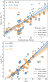 |
Fig. B.2 Speed-time relation (top panel, similar as Fig. 4) and Radialcomponent-distance relation (bottom panel, similar as Fig. 5), with φ Lup (blue) or SC15 (orange) as reference points. For comparison, we also show the slopes when e Lup is set as the reference point, from Fig. 4 or 5 (dashed black lines). The resulting median slopes are given in the upper left corners in the respective colours (see also Table 1). The shaded areas show the 1σ uncertainties around the median slopes. |
Finally, we tested if the speed-time relation is indeed linked to the formation time, as suggested by the linear trends when ordering the clusters by age and when using older clusters as reference points (Figs. 4 & B.2). To this end, we randomised the order of the time axis, while keeping the speed order as calculated for a given reference point. We set each of the 32 clusters once as a reference point, while the reference cluster was then removed from the correlation. We tested if the time-ordered relations are significant by randomly shuffling the measured formation times (or cluster ages) on the x-axis. Additionally, we created a uniform distribution of times between the formation time limits of the Sco-Cen clusters, (−20.9, −3.4) Myr, to create cases that are within the physical boundaries of the observed case. This allowed us to determine the linear regression statistics. For a more robust test, we determined the SRCC, which ranks the order of the values on the x and y axis, making it independent of the true physical scale. We find that the results from the timeordered cases - with e Lup, φ Lup, or SC15 as reference point -are only reproduced with a probability that is beyond 4σ. The positive linear correlation of time versus speed is not reproduced by the vast majority of the randomly ordered cases. About half of the random cases show negative trends (reversed slopes), which we also find when setting some of the mostly younger clusters as reference point (concerning Pipe-N, Musca-fg, η Cham, e Cham, TWA-a,b, δ Sco, ν Sco, ρ Oph, and B59). This test supports the hypothesis that the time-ordered behaviour of the motions in Sco-Cen, where younger clusters move faster compared to older ones, is unlikely to have been created by a random process in which clusters would form independently from each other, but it lies at the bottom of the formation history of the region.
Appendix C Online material
An overview of the columns of our stellar source catalogue is given in Table C.1 (available on Vizier), containing all 13,011 sources discussed in this paper. The table provides information on cluster labels and names, ages, the selected RV data, and derived parameters. The finally used RV value is either the measurement with the lowest RV uncertainty or the only available RV measurement (named vhel_best). The reference column (rv_ref) indicates from which survey the RV measurement originates (see Table A.1). Additionally, we give the weighted mean and weighted standard deviation if a source was observed by more than one RV survey (vhel_w_mean, vhel_w_std). We also list the individual RV data from all surveys mentioned in Table A.1, including the scatter parameter from MWM if available (std_v_rad), and the corrected RV uncertainties, if applicable (see Appendix A.3). Finally, we list derived parameters, including XYZ and UVW (see Appendix A.2). We flag the sources that pass our quality criteria to facilitate the selection of the used data: for the 5D sample, used_xzy = 1; and for the 6D sample, used_uvw = 1.
Source catalogue containing all 13011 sources discussed in this work. The Table is only available online on Vizier.
An overview of the columns of the cluster catalogue is given in Table C.2 (available on Vizier), listing parameters for the 36 clusters as given in Table A.2. We provide cluster properties, such as average positions and motions - median, mean, standard deviation (std), and their uncertainties - as obtained via bootstrapping (see Appendix B.3).
Finally, in Table C.3 (available on Vizier) we list the medians and uncertainties of the cumulative σ3D and the cumulative size for each age step, as used to construct Figs. 1, 3, and B.1.
Cumulative σ3D and cumulative size data (available on Vizier), used to create Figs. 1, 3, and B.1. We give the median and the uncertainties from the upper and lower 95th interquartile range (2σ) at each step. In the online version, the σ3D values are given for all four cumulative trends that are shown in Fig. B.1 and outlined in Appendix B.1.
All Tables
Overview of 36 stellar clusters toward Sco-Cen from R23a (SigMA selected clusters) and MR25 (TWA clusters), including RV data statistics, sorted by cluster age. An extended online version of this table is available on Vizier, which also contains further cluster properties, such as average positions and motions, as shown in the column overview in Table C.2.
Results of the total σ3D of the whole Sco-Cen association when using the different, mentioned data samples.
Source catalogue containing all 13011 sources discussed in this work. The Table is only available online on Vizier.
Cumulative σ3D and cumulative size data (available on Vizier), used to create Figs. 1, 3, and B.1. We give the median and the uncertainties from the upper and lower 95th interquartile range (2σ) at each step. In the online version, the σ3D values are given for all four cumulative trends that are shown in Fig. B.1 and outlined in Appendix B.1.
All Figures
|
Fig. 1 Cumulative 3D velocity dispersion of Sco-Cen, ordered by decreasing cluster age. The shaded orange area shows the 95% interquartile ranges (2σ bound), highlighting the uncertainties of the trend (see Appendix B.1). The symbols are coloured by the formation time of the youngest cluster included in the cumulative calculation (colour correlates with x-axis). We indicate the lookback time at the top of the x-axis, since the cumulative σ3D could also be interpreted as the evolution of velocity dispersion over time. The four vertical grey bars indicate the four main star formation events in Sco-Cen, marking four periods of an increased star formation rate, as is discussed in R23b (see their Fig. 3). |
| In the text | |
|
Fig. 2 3D spatial distribution of clusters in Sco-Cen together with the cumulative σ3D. The seven panels show seven age ranges, which dissect the chronological build-up of Sco-Cen. The upper panels display the cumulative 3D velocity dispersion (as in Fig. 1). Below each graph, seven 3D age maps depict the present-day spatial distribution of clusters (in XYZ). The clusters are represented by their enveloping surfaces and colour-coded by age. Each of the seven panels only shows the clusters that formed before the indicated cluster formation times. The shown cluster sizes can be interpreted as upper limits of the region’s size at a given age and not as the true physical extent before the present-day, which was likely smaller (see Sect. 5.4). The figure illustrates which clusters contribute to which jumps or steps in the cumulative σ3D. Sub-regions and cluster chains are labelled in the final panel. The 3D visualisations originate from R23b and MR25; interactive versions are available in the respective publications. |
| In the text | |
|
Fig. 3 Present-day cumulative size of Sco-Cen, when ordering and adding the stellar cluster members by their decreasing age (without considering orbital trace-backs). The sizes can be seen as upper limits of the region’s size at a given age, but not as the true physical extent before the present-day, which was likely smaller (see Sect. 5.4). The shaded green area shows the 95% interquartile range (2σ; see Appendix B.2). The colours and grey bars are as in Fig. 1. |
| In the text | |
|
Fig. 4 Speed-time relation. Relative cluster speed (v) versus lookback time (t), with the oldest cluster (e Lup) as a reference point that is excluded from the linear fit (dashed black circle). The symbols are colour-coded by formation time (or cluster age; see the x-axis) and scaled by number of sources per cluster. The linear fit (solid grey line) was obtained via bootstrapping, with the median fitting parameters given in the upper left corner. The fit uncertainties are plotted as shaded grey areas (1-2-3 σ). |
| In the text | |
|
Fig. 5 Radial-motion-distance relation. Radial component of the relative cluster motions (vr) versus relative cluster distance (r), with e Lup as a reference point. The symbols are colour-coded by formation time, as in Fig. 4. A linear fit to the data is shown as a solid grey line, with the best-fitting slope given in the upper left corner, and the 1-2-3σ fit uncertainties are plotted as shaded grey areas. The two clusters marked by dashed black circles (e Lup, ν Cen) are excluded from the linear fit. |
| In the text | |
|
Fig. 6 Position velocity (PV) diagrams for the 32 Sco-Cen clusters using the XU, YV, and ZW spaces. Symbols and colours as in Fig. 4. The median slopes of the fitted linear regressions (solid black lines) are given in the upper left corners. The shaded grey areas are the 1-2-3σ uncertainty ranges. The inverse of the slope gives a time in million years, in brackets, marking the possible onset of expansion. The dashed red slopes are the linear fitting results when using only 25 clusters, after removing seven clusters with peculiar tangential motions, marked with red circles (see Sect. 5.2). In the ZW diagram (right panel), the vertical dashed grey line indicates the approximate location of the Galactic mid-plane, assuming that the Sun is located about 21 pc above the plane (e.g. Bennett & Bovy 2019). |
| In the text | |
|
Fig. 7 Radial component of the relative cluster motions (vr) versus the tangential component (vtan) (left panel), and versus formation time (right panel), with e Lup as a reference point. Symbols and colours are as in Fig. 4. The dashed grey line in the left panel is a 1-to-1 line. The dashed dark grey line in the right panel shows a linear fit to data of 23 clusters, after removing the seven red-circled and the two dashed black-circled clusters. The solid light grey line at vr = 0 in both panels marks the transition from radial outward motion (> 0) to inward motion (< 0). |
| In the text | |
|
Fig. 8 Relative cluster distances versus formation time, with e Lup as a reference point. Symbols and colours as in Fig. 4. Two linear relations are fitted, once for all clusters (dashed light grey line) and once for 25 clusters (solid black line) after removing the seven red-circled clusters; see also Fig. 7. The shaded grey areas show the 1-2σ uncertainty ranges around the median slope when using 25 clusters. |
| In the text | |
|
Fig. B.1 Influence of measurement errors or binaries on the cumulative σ3D. (1) The upper orange curve is the fiducial one from Fig. 1. (2) The dashed black curve shows the cumul. σ3D when applying a cut on the Gaia RUWE parameter, to test the influence of binaries. (3) The middle blue curve shows the cumul. σ3D when applying an additional error cut at eRV ≤ 1 km s−1 on the stellar members of each cluster. (4) The magenta curve shows the cumul. σ3D when using the cluster medians. (5) The black cross marks the total σ3D as calculated from all stars in Sco-Cen with valid RV measurements. The error bars (shaded regions) show the 95% interquartile ranges (2σ). |
| In the text | |
|
Fig. B.2 Speed-time relation (top panel, similar as Fig. 4) and Radialcomponent-distance relation (bottom panel, similar as Fig. 5), with φ Lup (blue) or SC15 (orange) as reference points. For comparison, we also show the slopes when e Lup is set as the reference point, from Fig. 4 or 5 (dashed black lines). The resulting median slopes are given in the upper left corners in the respective colours (see also Table 1). The shaded areas show the 1σ uncertainties around the median slopes. |
| In the text | |
Current usage metrics show cumulative count of Article Views (full-text article views including HTML views, PDF and ePub downloads, according to the available data) and Abstracts Views on Vision4Press platform.
Data correspond to usage on the plateform after 2015. The current usage metrics is available 48-96 hours after online publication and is updated daily on week days.
Initial download of the metrics may take a while.