| Issue |
A&A
Volume 699, July 2025
|
|
|---|---|---|
| Article Number | A109 | |
| Number of page(s) | 21 | |
| Section | Extragalactic astronomy | |
| DOI | https://doi.org/10.1051/0004-6361/202554163 | |
| Published online | 02 July 2025 | |
Constraints on the state of the intergalactic medium at z∼8 − 10 using redshifted 21 cm observations with LOFAR
1
Department of Physical Sciences, Indian Institute of Science Education and Research Kolkata, Mohanpur, WB 741 246, India
2
Kapteyn Astronomical Institute, University of Groningen, PO Box 800 9700AV Groningen, The Netherlands
3
ARCO (Astrophysics Research Center), Department of Natural Sciences, The Open University of Israel, 1 University Road, PO Box 808 Ra’anana 4353701, Israel
4
Max-Planck Institute for Astrophysics, Karl-Schwarzschild-Straße 1, 85748 Garching, Germany
5
The Oskar Klein Centre, Department of Astronomy, Stockholm University, AlbaNova, SE-10691 Stockholm, Sweden
6
Van Swinderen Institute for Particle Physics and Gravity, University of Groningen, Nijenborgh 4, 9747 AG Groningen, The Netherlands
7
Nordita, KTH Royal Institute of Technology and Stockholm University, Hannes Alfvéns väg 12, SE-106 91 Stockholm, Sweden
8
LUX, Observatoire de Paris, PSL Research University, CNRS, Sorbonne Université, F-75014 Paris, France
9
Astron, PO Box 2 7990 AA Dwingeloo, The Netherlands
10
Astronomy Centre, Department of Physics and Astronomy, Pevensey II Building, University of Sussex, Brighton BN1 9QH, UK
11
INAF – Istituto di Radioastronomia, Via P. Gobetti 101, 40129 Bologna, Italy
12
Laboratoire de Physique de l’ENS, ENS, Université PSL, CNRS, Sorbonne Université, Universitée Paris Cité, 75005 Paris, France
13
School of Physics and Electronic Science, Guizhou Normal University, Guiyang 550001, PR China
14
Department of Computer Science, University of Nevada, Las Vegas, Nevada 89154, USA
15
Center for Fundamental Physics of the Universe, Department of Physics, Brown University, Providence, 02914 RI, USA
⋆ Corresponding author: This email address is being protected from spambots. You need JavaScript enabled to view it.
Received:
17
February
2025
Accepted:
1
May
2025
Abstract
The power spectra of the redshifted 21 cm signal from the Epoch of Reionization (EoR) contain information about the ionization and thermal states of the intergalactic medium (IGM) and depend on the properties of the sources that existed during that period. Recently, the LOFAR-EoR Key Science Project team has analysed ten nights of LOFAR high-band data and estimated upper limits on the 21 cm power spectrum at redshifts 8.3, 9.1, and 10.1. Here, we used these upper limit results to constrain the properties of the IGM at those redshifts. We focus on the properties of the ionized and heated regions where the temperature is larger than that of the cosmic microwave background (CMB). We modelled the power spectrum of the 21 cm signal with the code GRIZZLY and used a Bayesian inference framework to explore the source parameters for uniform priors on their ranges. The framework also provides information about the IGM properties in the form of derived parameters. We do not include constraints from other observables except for some very conservative limits on the maximum ionization fraction at those redshifts, which we estimated from the CMB Thomson scattering optical depth. In a model that includes a radio background in excess of the CMB, the 95% (68%) credible intervals of disfavoured models at redshift 9.1 for the chosen priors correspond to IGM states with an averaged ionization and heated fraction below 0.46 (≲ 0.05), an average gas temperature below 44 K (4 K), and a characteristic size of the heated region of ≲14 h−1 Mpc (≲3 h−1 Mpc). The 68% credible interval suggests an excess radio background that is more than 100% of the CMB at 1.42 GHz, while the 95% credible interval of the radio background efficiency parameter spans the entire prior range. The behaviour of the credible intervals is similar at all redshifts. The models disfavoured by the LOFAR upper limits are extreme, as they are mainly driven by rare and large ionized or heated regions. We find that the inclusion of upper limits from other radio interferometric observations in the Bayesian analysis significantly increases the number of disfavoured EoR models, thus enhancing the disfavoured credible intervals of the IGM parameters, especially those related to the average gas temperature and size distribution of the heated regions. While our constraints are not yet very strong, more stringent upcoming results from 21 cm observations together with the detection of many high-z galaxies, for example with the James Webb Space Telescope, will strengthen understanding of this crucial phase of the Universe.
Key words: radiative transfer / galaxies: formation / galaxies: high-redshift / intergalactic medium / cosmology: theory / dark ages / reionization / first stars
© The Authors 2025
 Open Access article, published by EDP Sciences, under the terms of the Creative Commons Attribution License (https://creativecommons.org/licenses/by/4.0), which permits unrestricted use, distribution, and reproduction in any medium, provided the original work is properly cited.
This article is published in open access under the Subscribe to Open model. This email address is being protected from spambots. You need JavaScript enabled to view it. to support open access publication.
1. Introduction
The formation of the first stars and galaxies transformed the Universe from a cold and neutral phase to a hot and highly ionized one. The era when ultraviolet (UV) radiation from the earliest sources ionized the neutral hydrogen (H I) in the intergalactic medium (IGM) is known as the Epoch of Reionization (EoR). While concrete evidence for the existence of this phase transition exists, its details remain unknown. Several observational probes, such as the CMB Thomson scattering optical depth (e.g. Planck Collaboration VI 2020), high-redshift (z) Lyα emitters (e.g. Hu et al. 2010; Morales et al. 2021; Tang et al. 2023; Witten et al. 2024), the Gunn-Peterson trough, and the Lyα damping wings in high-z quasar spectra (e.g. Fan et al. 2006; Becker et al. 2015; Bañados et al. 2018), have provided limited but useful insight about the evolution of the average neutral fraction.
Currently, the redshifted 21 cm signal from neutral hydrogen is the most promising observational probe of the spatial distribution and temporal evolution of H I in the IGM (see e.g. Madau et al. 1997; Furlanetto et al. 2006; Zaroubi 2013). This signal carries a large amount of information on the physical state of the IGM as well as on the properties of the first UV and X-ray emitting sources. Indeed, as it is a line emission, the 21 cm signal permits one to study physical processes at different stages of the EoR.
To measure the redshifted 21 cm signal, several radio observations have been set up or proposed, and they can be divided into two categories. The first type uses a single radio antenna and attempts to measure the time evolution of the sky-averaged brightness temperature ( ) of the 21 cm signal. Into this category fall instruments such as the Experiment to Detect the Global EoR Signature (EDGES; Bowman & Rogers 2010), EDGES2 (Monsalve et al. 2017; Bowman et al. 2018), the Shaped Antenna measurement of the background RAdio Spectrum (SARAS; Patra et al. 2015), SARAS2 (Singh et al. 2017), the Broadband Instrument for Global HydrOgen Reionization Signal (BigHorns; Sokolowski et al. 2015), the Sonda Cosmologica de las Islas para la Deteccion de Hidrogeno Neutro (SciHi; Voytek et al. 2014), the Large Aperture Experiment to detect the Dark Ages (LEDA; Price et al. 2018), the Radio Experiment for the Analysis of Cosmic Hydrogen (REACH; de Lera Acedo et al. 2022), Probing Radio Intensity at High-Z from Marion (Prizm; Philip et al. 2018), and the Mapper of the IGM Spin Temperature (MIST; Monsalve et al. 2024).
The second type uses large radio interferometers to measure the spatial fluctuations of the redshifted H I signal in a statistical sense, mainly through its power spectrum. To this category belong ongoing or completed observations such as the Low Frequency Array (LOFAR1; van Haarlem et al. 2013; Patil et al. 2017), the Giant Metrewave Radio Telescope (GMRT; Paciga et al. 2013), the Precision Array for Probing the Epoch of Reionization (PAPER2; Parsons et al. 2014; Kolopanis et al. 2019), the Murchison Widefield Array (MWA3; Tingay et al. 2013), the Hydrogen Epoch of Reionization Array (HERA4; DeBoer et al. 2017), and the New Extension in Nançay Upgrading LOFAR (NenuFAR5; Munshi et al. 2024). Around the start of the next decade, the Square Kilometre Array (SKA)6 will become available, and its transformative sensitivity should also enable tomographic imaging of the signal (Mellema et al. 2013, 2015; Koopmans et al. 2015; Ghara et al. 2017).
These observations face a range of challenges. Among them is the mitigation of the galactic and extra-galactic foregrounds, which are four to five orders of magnitude brighter than the expected signal (see e.g. Ghosh et al. 2012). However, the smooth frequency dependence of the foreground signal allows for its subtraction (Harker et al. 2009; Bonaldi & Brown 2015; Chapman et al. 2016; Mertens et al. 2018; Hothi et al. 2021), avoidance (Datta et al. 2010; Liu et al. 2014), or suppression (Datta et al. 2007; Ghara et al. 2016). At the same time, an accurate calibration during the data analysis process is required to minimise the artefacts from bright foreground sources (Barry et al. 2016; Patil et al. 2017). Recent improvements in foreground mitigation algorithms (e.g. Liu et al. 2014; Mertens et al. 2018, 2024; Acharya et al. 2024a; Gao et al. 2024), calibration methods (see e.g. Yatawatta & Banerjee 2011; Kern et al. 2019, 2020; Mevius et al. 2022; Gan et al. 2022, 2023), mitigation of radio frequency interference (see e.g. Offringa et al. 2019; Wilensky et al. 2019; Munshi et al. 2025), and ionospheric effects (e.g. Mevius et al. 2016; Edler et al. 2021), as well as improved sky-model building (see e.g. Patil et al. 2016; Ewall-Wice et al. 2017) and inclusion of polarisation effects (e.g. Jelić et al. 2010; Spinelli et al. 2018) in the data analysis step, are showing promising results in reducing the effects of systematics and in helping recover the targeted 21 cm signal.
So far only one detection of  with a minimum at z ≈ 17 (Bowman et al. 2018) has been claimed based on an EDGES2 low-band observation. This detection, though, remains disputed (e.g. in Hills et al. 2018; Draine & Miralda-Escudé 2018; Singh & Subrahmanyan 2019; Bradley et al. 2019), and it requires confirmation from other similar observations. A recent observation in the 55-85 MHz band with SARAS3 is inconsistent with the results from Bowman et al. (2018), ruling out the deep
  profile around z ∼ 17 with 95% confidence (Singh et al. 2022). Other global 21 cm signal experiments, such as LEDA (Bernardi et al. 2016), EDGES high-band (Monsalve et al. 2017, 2019), and SARAS2 (Singh et al. 2017), have only provided upper limits on the signal amplitude. Results from SARAS and EDGES, however, have started ruling out EoR scenarios and putting constraints on the early source properties, dark matter models, and the strength of the radio background (e.g. Barkana 2018; Fialkov et al. 2018; Muñoz & Loeb 2018; Nebrin et al. 2019; Chatterjee et al. 2019, 2020; Ghara & Mellema 2020; Ghara et al. 2022; Bera et al. 2023; Acharya et al. 2023; Cyr et al. 2024).
This paper focuses on the results of radio interferometric observations of the 21 cm signal power spectrum Δ2, which contains much more information than the global signal. At the current time, such observations have only produced upper limits. A 2σ upper limit of (248)2 mK2 for k = 0.5 h Mpc−1 at z = 8.6 from the GMRT was the first of its kind (Paciga et al. 2013). Later, PAPER7 (Parsons et al. 2014; Ali et al. 2015), LOFAR (Patil et al. 2017; Mertens et al. 2020), MWA (Barry et al. 2019; Trott et al. 2020), and HERA (Abdurashidova et al. 2023) produced additional upper limits. To date, Δ2(k = 0.075 h Mpc−1, z = 9.1, 141 hours)≈(73)2 mK2, Δ2(k = 0.34 h Mpc−1, z = 7.9, 1128 hours)≈(21.4)2 mK2, and Δ2(k = 0.14 h Mpc−1, z = 6.5, 110 hours)≈(43)2 mK2 are the best upper limits obtained from LOFAR (Mertens et al. 2020), HERA (Abdurashidova et al. 2023), and MWA (Trott et al. 2020) EoR observations, respectively. Recent observations with the LOFAR-Low Band Antenna array (Gehlot et al. 2019), the Owens Valley Radio Observatory Long Wavelength Array (OVRO-LWA; Eastwood et al. 2019), and NenuFAR (Munshi et al. 2024) have produced upper limits at higher redshifts. These data have been used to rule out not only some unusual reionization scenarios requiring, for example, atypical cooling mechanisms or the presence of a radio background in addition to the CMB, but also less exotic ones (see e.g. Ghara et al. 2020; Greig et al. 2021; Mondal et al. 2020; Abdurashidova et al. 2022).
Mertens et al. (2025) have recently published new results from the LOFAR team in the redshift range of 8.3–10.1, with a best 2σ upper limit of Δ2(k = 0.076 h Mpc−1, z = 9.1, 140 hours)≈(54.3)2 mK2. This is approximately a factor of two improvement at the same k− scale and redshift in comparison to the previous one from Mertens et al. (2020) and thus is expected to rule out even more EoR scenarios than those already excluded in Ghara et al. (2020), Greig et al. (2021), and Mondal et al. (2020). Additionally, the upper limits at the other two redshifts might help in ruling out even more EoR scenarios.
It should be noted that the 21 cm signal measurements do not directly probe astrophysical sources but rather the ionization and thermal state of the IGM. However, presenting the 21 cm signal observables in terms of IGM-related parameters is challenging (see e.g. Mirocha et al. 2022; Ghara et al. 2024; Choudhury et al. 2024). As the 21 cm signal simulation codes use the source parameters as input, previous studies mainly focused on constraining the astrophysical source properties using either Fisher matrices or Bayesian inference techniques (e.g. Ewall-Wice et al. 2016; Park et al. 2019; Cohen et al. 2020). It should be noted that the inference on the astrophysical source properties is limited by the assumptions of the source model used in the 21 cm signal simulation codes. We therefore put less emphasis on the inference results for the source parameters and focus on the IGM properties instead.
In this paper, we use the new LOFAR upper limits to investigate which EoR scenarios are disfavoured within the redshift range of 8.3–10.1. We achieved this by employing the Bayesian inference framework previously used in Ghara et al. (2021) to interpret multi-redshift upper limits from MWA observations (Trott et al. 2020). The main difference between this version of the framework and the one used in Ghara et al. (2020) is that we consider the presence of an excess radio background component in addition to the CMB, similar to what was done in Mondal et al. (2020).
The paper is structured as follows. In Sect. 2, we describe the new LOFAR upper limits used in this study and introduce the basic methodology of our Bayesian interpretation framework. We present our results in Sect. 3, and finally we conclude our study in Sect. 4. We adopted the cosmological parameters Ωm = 0.27, ΩΛ = 0.73, ΩB = 0.044, and h = 0.7 (Wilkinson Microwave Anisotropy Probem WMAP; Hinshaw et al. 2013), which are the same as used in the N-body simulations employed here.
2. Methodology
Here we briefly describe the new LOFAR upper limits on the 21 cm signal power spectrum. We also give an overview of the framework employed to constrain the IGM properties with them.
2.1. Observations
The LOFAR-EoR Key Science Project team has analysed data for the North Celestial Pole (NCP) field from 14 nights of observations taken during LOFAR Cycles 0–3. Previously, Mertens et al. (2020) analysed 12 nights (resulting in 141 hours) of NCP data in the frequency range 134–146 MHz, and presented upper limits on the 21 cm signal power spectrum at z = 9.1. In the latest results, the team has added two more nights at 134–146 MHz (z = [8.73, 9.6]), and also analysed two additional frequency bands: 122–134 MHz (z = [9.6, 11.64]) and 146–158 MHz (z = [8, 8.73]), while only the best 10 nights (corresponding to 140 hours) of data for each redshift bin are finally combined. This has resulted in new upper limits on the 21 cm signal power spectrum at z = 8.3, 9.1 and 10.1.
The details of the observations and the analysis techniques can be found in Mertens et al. (2025). Here we summarise the final results in Table 1. It shows the mean power spectrum Δ212(k, z) and associated 1σ error Δ21, err2(k, z). The best result is at z = 9.1, with a 2σ upper limit of (54.3 mK)2 at k = 0.075 h Mpc−1, which is a factor of ≈2 lower than the one reported in Mertens et al. (2020). This is caused by improvements in the data analysis pipeline (see Mertens et al. 2025 for more details).
Recent LOFAR upper limit on Δ2 at different k-bins for z = 8.3, 9.1, and 10.1.
2.2. Interpretation framework
The framework employed to constrain the IGM properties using the upper limit results from Mertens et al. (2025) relies on a large (∼105) database of reionization scenarios, as well as the associated IGM properties and 21 cm signal power spectra. These theoretical power spectra are then used in a Bayesian analysis in combination with the measured ones to find the exclusion likelihood for a reionization scenario. The same approach was used in Ghara et al. (2021) to interpret upper limits from observations with MWA. We refer the reader to Ghara et al. (2020, 2021) for a detailed description of the framework.
The large database of reionization scenarios and associated 21 cm signals is produced with GRIZZLY (Ghara et al. 2015a, 2018), an independent implementation of the BEARS algorithm (Thomas & Zaroubi 2008; Thomas et al. 2009; Thomas & Zaroubi 2011; Krause et al. 2018). It requires cosmological density and velocity fields, together with the dark matter halo catalogues as input. These are typically obtained from a cosmological N-body simulation. Given a set of astrophysical source parameters, it then employs a one-dimensional radiative transfer scheme to generate ionization fraction, gas temperature and Lyα flux fields. The N-body simulation as well as the source model used in GRIZZLY are described in the following sub-sections.
2.2.1. N-body simulation
The N-body outputs used here are the same employed in Ghara et al. (2020) and were obtained from the PRACE8 project PRACE4LOFAR. The dark matter-only simulation was run using the cubep3m (Harnois-Déraps et al. 2013) code with particle mass resolution of 4.05 × 10⁷ M⊙. The simulation cube has a size of 500 h−1 Mpc, corresponding to a field-of-view of 4.3° ×4.3° at z≈ 9. This length is enough to cover the largest scale probed by the LOFAR observations, which corresponds to a k-scale of 0.05 h Mpc−1, requiring a size of at least ≈250 h−1 Mpc.
The density and velocity fields were smoothed onto a 3003 grid (see e.g, Giri et al. 2019a,b). The lists of dark matter halos were obtained on the fly during the N-body simulation using a spherical overdensity halo finder (Watson et al. 2013). The halo lists consist of halos with more than 25 particles, which leads to a minimum dark matter halo mass ≈109 M⊙.
2.2.2. GRIZZLY source model
The next step is to employ GRIZZLY (Ghara et al. 2015a, 2018) to generate 3D cubes of the 21 cm signal at the probed redshifts. For this, we used different combinations of astrophysical parameters, which encode the source properties in terms of the emissivity of UV, X-ray, Lyα, and radio photons, as each of these affects the spatial fluctuations of the signal (see e.g. Ross et al. 2019; Eide et al. 2020; Reis et al. 2020). Our source model assumes that the stellar mass M⋆ in a dark matter halo with mass Mhalo is  , where f⋆ is the star formation efficiency. In all our simulations we used f⋆ = 0.02, which is consistent with studies such as Behroozi & Silk (2015) and Sun & Furlanetto (2016).
The source parameters we varied to create our set of simulations are as follows:
(1) Ionization efficiency (ζ): This parameter regulates the emission rate of ionizing photons escaping into the IGM from a halo9. We assume it to be constant per unit stellar mass, or in other words, this emission rate scales linearly with halo mass. The rate is then given by  , where we vary log10(ζ) in the range [–3, 3].
(2) X-ray heating efficiency (fX): This is the parameter that regulates the emission rate of X-ray photons from a halo according to  , where we consider the X-ray band to span from 100 eV to 10 keV. Just as the ionizing ultraviolet radiation, the X-ray emission scales linearly with halo mass. We adopt a power-law spectral energy distribution (SED), i.e. IX(E)∝E−α, where α = 1.2 across the X-ray band. The
  value for fX = 1 is in agreement with the SED of high-mass X-ray binaries in local star-forming galaxies for the 0.5–8 keV band (Mineo et al. 2012; Islam et al. 2019). We vary log10(fX) in the range [–3, 3].
(3) Minimum mass of UV emitting halos (Mmin): This parameter determines the number density of UV emitting sources, as we assume that only dark matter halos with a mass larger than Mmin contribute to the ionizing photon budget. We vary log10(Mmin/M⊙) in the range [9, 12]. The lower value is determined by the lowest mass halos resolved in our N-body simulations. While the number density of dark matter halos in a ΛCDM cosmology is larger at the low mass end, star formation in halos with mass ≲ 109 M⊙ is expected to be significantly suppressed due to thermal feedback, SNe feedback, or inefficient gas accretion (see e.g. Shapiro et al. 1994; Barkana & Loeb 2001; Springel & Hernquist 2003; Sobacchi & Mesinger 2013). These lower mass halos are therefore expected to have a less significant impact on the 21 cm signal power spectrum.
(4) Minimum mass of X-ray emitting halos (Mmin, X): This determines the number density of X-ray emitting halos, as we assume that only halos with a mass larger than Mmin, X host X-ray sources. Also for log10(Mmin, X/M⊙) we explore the range [9, 12].
(5) Radio background efficiency (Ar): We assumed the existence of a radio background10 in addition to the CMB. This parameter quantifies the effective brightness temperature of the total radio background as (Fialkov & Barkana 2019; Mondal et al. 2020)
![Mathematical equation: $$ \begin{aligned} {T_{\gamma , {\mathrm{eff} }}} = T_{\gamma } \left[1+A_r \left(\frac{\nu _{\rm obs}}{78\,\mathrm{MHz}} \right)^{-2.6} \right]. \end{aligned} $$](/articles/aa/full_html/2025/07/aa54163-25/aa54163-25-eq8.gif) (1)
(1)
Here, Tγ(z) = 2.725 (1 + z) K is the usual CMB temperature and νobs is the observation frequency. For simplicity, we adopt a uniform radio background, but the presence of inhomogeneities could enhance the amplitude of the 21 cm signal power spectrum above our estimates (Reis et al. 2020). We vary Ar in the range [0, 416]. The lower bounds correspond to no excess radio background (i.e. Tγ, eff = Tγ), while the upper bounds represent the upper limits of 0.603 K as measured by LWA1 (Dowell & Taylor 2018).
2.2.3. Simulating the 21 cm signal power spectrum
The 21 cm signal brightness temperature (δTb) can be written as (see e.g, Madau et al. 1997; Furlanetto et al. 2006)
![Mathematical equation: $$ \begin{aligned} {\delta T_{\mathrm{b} }} (\mathbf x , z) \!&= \! 27 ~ x_{\rm HI} (\mathbf x , z) [1+\delta _{\rm B}(\mathbf x , z)] \left(1-\frac{{T_{\gamma , {\mathrm{eff} }}}(z)}{{T_{\mathrm{S} }}(\mathbf x , z)} \right) \nonumber \\&\quad \times \! \left(\frac{{\Omega _{\mathrm{B} }} h^2}{0.023}\right) \left(\frac{0.15}{{\Omega _{\mathrm{m} }} h^2}\frac{1+z}{10}\right)^{1/2} \left(\frac{H}{\mathrm{d} v_\mathrm{r} /\mathrm{d} r+H}\right)\,\mathrm{mK}. \end{aligned} $$](/articles/aa/full_html/2025/07/aa54163-25/aa54163-25-eq9.gif) (2)
(2)
Here, [1 + δB(x, z)] is the overdensity at position x and redshift z, extracted from the gridded density fields obtained from the N-body simulation described in Sect. 2.2.1. The quantities xHI, TS, H and dvr/dr are the neutral hydrogen fraction, the spin temperature of hydrogen in the IGM, the Hubble parameter and the velocity gradient along the line of sight, respectively. Given a set of astrophysical source parameters, GRIZZLY generates xHI and gas temperature (TK) maps. Here, we assume TS = TK which is expected at the redshifts of interest due to the presence of a strong Lyα background (e.g. Barkana & Loeb 2005; Pritchard & Loeb 2012; Schneider et al. 2021). We include the line-of-sight velocity field effects (so-called redshift space distortions, RSD) to the δTb cubes using the cell movement method (or Mesh-to-Mesh Real-to-Redshift-Space-Mapping scheme; Mao et al. 2012; Ghara et al. 2015b; Ross et al. 2021). Finally, we estimate the dimensionless power spectrum of δTb, denoted as Δ2(k)11.
2.2.4. Derived IGM parameters
Similar to Ghara et al. (2020, 2021), our main focus here is on the characterisation of the IGM, as its properties are directly linked to the observed 21 cm signal. However, our framework is not completely independent of source models, as GRIZZLY uses a set of source parameters as input to simulate ionization and temperature fields, which are then used to determine a set of quantities related to the IGM.
When considering the IGM parameters, we defined ‘heated regions’ as those with TK > Tγ, eff. To derive the size distribution of these regions, we used the mean free path (MFP) method from Mesinger & Furlanetto (2007), see Ghara et al. (2020) for more details. We then considered the following derived IGM parameters or quantities12 for each redshift:
-
 : Volume-averaged ionized fraction.
 -
 (K): Volume-averaged gas temperature of neutral regions, where we consider the gas to be neutral if xHII < 0.5. We note that choosing a different value would change the estimate of
  . In general, a higher xHII threshold results in a larger value of
  .
. -
 (mK): Mass-averaged differential brightness temperature.
 -
fheat: Volume fraction of heated regions (TK > Tγ, eff).
-
 (h−1 Mpc): Characteristic size of the heated regions, corresponding to the size at which the distribution of heated regions size peaks.
 -
 (h−1 Mpc): Full width at half maximum (FWHM) of the PDF of the size distribution of heated regions.
2.2.5. Bayesian inference
To explore the source parameter space as given in Table 2, we use the publicly available Markov chain Monte Carlo (MCMC) sampler code COBAYA13 (Lewis & Bridle 2002). The likelihood of a set of parameters θ to be excluded at z for an upper limit of the power spectrum Δ212(ki, z)±Δ21, err2(ki, z), can be defined as (see Ghara et al. 2020, for details)
![Mathematical equation: $$ \begin{aligned} \mathcal{L} _{\mathrm{ex, single} -z}(\boldsymbol{\theta }, z) = 1- \prod _{i} \frac{1}{2}\left[ 1 + \mathrm{erf} \left(\frac{{\Delta ^2_\mathrm{21} } (k_i, z)- {\Delta ^2_\mathrm{m} }(k_i, \boldsymbol{\theta }, z)}{\sqrt{2} \sigma (k_i, z)}\right) \right]. \end{aligned} $$](/articles/aa/full_html/2025/07/aa54163-25/aa54163-25-eq17.gif) (3)
(3)
Overview of the source parameters used in GRIZZLY with their explored ranges.
Here, Δm2(k, θ, z) is the model power spectrum for a set of parameters θ, while σ is the error that includes contributions from the observational error (Δ21, err2) as well as from the power spectrum modelling error (Δm, err2):  .
.
Unlike our previous inference studies, here we also consider the combination of the three upper limits into a joint likelihood:
![Mathematical equation: $$ \begin{aligned} \mathcal{L} _{\mathrm{ex, joint} -z}(\boldsymbol{\theta }) = 1- \prod _{i,j} \frac{1}{2}\left[ 1 + \mathrm{erf} \left(\frac{{\Delta ^2_\mathrm{21} } (k_i, z_j)- {\Delta ^2_\mathrm{m} }(k_i, \boldsymbol{\theta }, z_j)}{\sqrt{2} \sigma (k_i, z_j)}\right) \right]. \end{aligned} $$](/articles/aa/full_html/2025/07/aa54163-25/aa54163-25-eq21.gif) (4)
(4)
We note that multiple upper limits can be combined into a single likelihood only when the redshift evolution of the source parameters is well understood. As here we assume the source parameters to be redshift-independent, some caution should be applied in the interpretation of the joint analysis. In the future, we plan to extend it by employing the code POLAR (Ma et al. 2023; Acharya et al. 2024b), which includes a redshift evolution in the modelling of the source parameters.
Similar to Ghara et al. (2021), our framework does not directly use GRIZZLY in the MCMC analysis. Instead, we first employ GRIZZLY to generate 105 sets of power spectra and IGM parameters at each of the three redshifts by sampling the 5D source parameter space14. Then, in the MCMC analysis we employ a linear interpolation scheme (Weiser & Zarantonello 1988; Virtanen et al. 2020) over the 5D source parameter space, which uses the previously generated power spectra and IGM parameters. We also consider a conservative 30% modelling error, Δm, err2(ki, z) = 0.3 × Δm2(ki, θ, z). This includes the inherent modelling errors due to the approximate nature of the GRIZZLY algorithm15, as well as the errors introduced by the interpolation scheme. To run the MCMC on the source parameters, we used ten walkers and 106 steps, and ensure that all the MCMC chains converge well before the final step. We adopt a uniform prior in log-scale on the explored parameter ranges (see Table 2). COBAYA produces the list of corresponding derived IGM parameters using the same linear interpolation scheme.
As the upper limits towards the largest k values exceed the values for all of the power spectra in our simulation database (see next section), they do not yield any constraints. Therefore, only the three smallest k-bins (see Table 1) are used in the MCMC analysis to estimate ℒex, single − z(θ, z) and ℒex, joint − z(θ).
In this analysis we also use a prior on  , derived from the measured Thomson scattering optical depth towards the CMB. For each of the three redshifts zi we assume a stepwise reionization history, in which the Universe is neutral until zi, partially ionized at a level (
 ) until redshift 6, and fully ionized after that16. The value
  follows from assuming the 1στ measurement, i.e. τ = 0.061 for τ = 0.054 ± 0.007 (Planck Collaboration VI 2020). It represents the largest possible of value of
  at redshift zi consistent with the τ measurements. We obtain values of
  , 0.79 and 0.57 at z = 8.3, 9.1 and 10.1, respectively. The same approach was used in Ghara et al. (2020, 2021). We note that in a realistic reionization scenario, the evolution of
  is expected to be gradual.
It should be noted that the Bayesian analysis explores the source parameters rather than the IGM parameters, as our framework uses the former as input. The source parameter values obtained from the MCMC chains are then used to generate lists of corresponding IGM parameter values. Finally, these lists are employed to obtain the posterior distribution of the IGM parameters. Because of this procedure, the constraint on the IGM parameters might be significantly affected by the priors on the source parameters. We discuss this in Appendix A.
3. Results
Before describing the quantitative analysis of our results, we present in Fig. 1, as an illustration, a subset of the 21 cm signal power spectra with Ar = 0 at z = 8.3, 9.1 and 10.1. We find that at each redshift some of the power spectra (indicated with coloured lines) have values larger than Δ212(k, z)−Δ21, err2(k, z) from the recent LOFAR 1σ upper limits from Mertens et al. (2025, indicated by the down arrow points) in at least one k-bin. For this reason, they have a high probability of being ruled out. Overall, we find that 10%, 13%, and 5% of our simulated power spectra fall into this category at z = 8.3, 9.1 and 10.1, respectively. Here it should be kept in mind that these fractions depend on the priors chosen for the source parameters. On the other hand, the power spectra in grey have a low exclusion probability as they remain below that limit. The thick dashed lines correspond to the power spectra of a completely neutral and unheated IGM, obtained assuming constant values of xHI = 1 and TS = TK = 0.021 × (1 + z)2 K. We note that the observed upper limits are still unable to rule out this scenario. We estimate that for z = 9.1 at least 2–3 times more integration time would be required to achieve that.
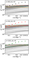 |
Fig. 1. Set of 1000 power spectra randomly chosen from the 105 simulated power spectra. Panels from top to bottom refer to z = 8.3, 9.1, and 10.1, respectively. These correspond to the scenario with no additional radio background other than the CMB (Ar = 0). The down arrow points refer to the recent LOFAR 1σ upper limit (Δ212(k, z)±Δ21, err2(k, z)) from Mertens et al. (2025). As a reference, the dashed line corresponds to the power spectrum for a completely neutral IGM with no X-ray heating, and with TS = TK. The coloured power spectra are those with a value larger than Δ212(k, z)−Δ21, err2(k, z) in at least one k-bin, i.e. they have a high probability of being ruled out, while those in grey have a low exclusion probability. |
As a further illustration, Fig. 2 shows the distribution of source parameters for models with a high probability of being ruled out, i.e. which have a value larger than Δ212(k, z)−Δ21, err2(k, z) in at least one k-bin. The vertical axes represent the number of disfavoured models out of the total of 105. We only consider the Ar = 0 scenario and each source parameter range has been logarithmically binned into eight bins. We note that a significant fraction of these disfavoured models has high values of Mmin and Mmin, X, indicating that they represent scenarios in which the ionized or heated regions are rare. A large fraction of models also has high values of ζ and fX, suggesting that the rare ionized or heated regions are large in size.
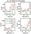 |
Fig. 2. Histogram of the disfavoured values of the source parameters for the scenario with Ar = 0. These correspond to the models with power spectra values larger than Δ212(k, z)−Δ21, err2(k, z) in at least one k-bin, and they have a high probability of being ruled out by the recent LOFAR 1σ upper limits (Δ212(k, z)±Δ21, err2(k, z)) from Mertens et al. (2025). |
In Fig. 3, we present the distribution of IGM parameters for the same set of models considered in Fig. 2. A significant number of disfavoured models at all redshifts have  and fheat smaller than ∼0.6. The characteristic sizes in these models are several tens of h−1 Mpc, indicating that the ionized or heated regions are both rare and large. At the same time, the volume occupied by them remains less than 50% of the total volume. We note that a large number of disfavoured models with
  , fheat ≲ 0.1 and
  K are strongly influenced by the priors chosen on the source parameters (see Appendix A for details).
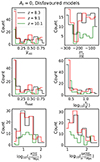 |
Fig. 3. Histogram of the disfavoured values of the IGM parameters for the scenario with Ar = 0. These correspond to the same set of models considered in Fig. 2. |
In the following sections, we present the results of our MCMC analysis. Following the same approach adopted in Ghara et al. (2021), we first perform the MCMC using the likelihood ℒex, single − z(θ, z) as given in Eq. (3), which accounts for upper limits at a single redshift only. We denote this as ‘Single-z’ analysis. We also run an MCMC analysis where we use the joint likelihood ℒex, joint − z(θ) as shown in Eq. (4), which combines all the upper-limit results. We denote this as ‘Joint-z’ analysis. We note again that as our source parameters are assumed to be redshift independent, the results of the Joint-z analysis should be interpreted with some caution. We first consider the case of no additional radio background and follow it by the case in which we allow for an additional radio background. Finally we describe how the inclusion of upper limits on the power spectrum from other 21 cm experiments impacts the results.
3.1. Analysis without excess radio background (Ar = 0)
For Ar = 0 our parameter space is 4D, defined by ζ, Mmin, Mmin, X and fX. This scenario corresponds to one in which the only radio background at 1420 MHz is the CMB.
Figure 4 shows the posterior distribution of the GRIZZLY source parameter space at z = 9.1. Here we highlight that the likelihood used in the MCMC represents the exclusion probability of a model. We also note that the 68% and 95% credible interval contours on the two-dimensional contour panels have remained open, indicating that the constraints on the source parameters depend on the chosen prior ranges. We find that the 68% disfavoured credible intervals17 from the Single-z analysis at z = 9.1 are  and
and  , while the limits for ζ and fX span the entire parameter ranges. The 95% disfavoured credible intervals of the source parameters span the entire parameter ranges for both the Single-z and Joint-z analysis. The 68% credible intervals for the Joint-z analysis case are similar to those of the Single-z case. One reason behind the similarity could be that the Joint-z analysis results are likely to be biased by the strongest upper limit results, which are at z = 9.1.
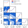 |
Fig. 4. Posterior distribution of the disfavoured values of the source parameters for the Ar = 0 scenario. These are disfavoured by the LOFAR upper limits from Mertens et al. (2025) at z = 9.1. Red refers to the case when each redshift is considered separately (Single-z) at z = 9.1, while blue represents the joint MCMC analysis results (Joint-z). The contour levels in the two-dimensional contour plots refer to the 1σ and 2σ credible intervals of the models disfavoured by the LOFAR upper limit at this redshift. The diagonal panels represent the corresponding marginalised probability distributions of each parameter. |
The marginalised probability distributions of the disfavoured source parameter values at all redshifts are shown in Fig. 5. The related credible intervals are listed in Table 3 for both the Single − z and Joint − z cases. The credible intervals for Mmin and Mmin, X for the three Single-z cases are qualitatively consistent with each other, as they disfavour models at the highest end of the prior range, i.e. log10(Mmin) or log10(Mmin, X)≳10.5 M⊙. This suggests that models associated with a low number density of massive UV and X-ray emitting sources are disfavoured. The limits for ζ, on the other hand, differ among the various redshifts. For z = 10.1 models towards the higher end of our prior interval are disfavoured, but for z = 8.3 it is rather models at the lower end of our prior interval which are found to be less likely. The same trend is seen for the fX parameter. This can be understood from the difference in the number density of halos between these two redshifts. Scenarios more likely to be disfavoured require a high contrast, so the ionized or heated regions should not be too small and few or too large and many. With a smaller halo density at z = 10.1, relatively large efficiencies are needed to produce a large contrast population of ionized or heated regions, but at the larger halo density for z = 8.3 such high efficiencies would ionize or heat too much of the IGM, yielding a low contrast, and instead lower efficiencies are needed to create a large contrast distribution of ionized or heated regions.
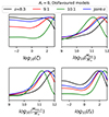 |
Fig. 5. Marginalised probability distribution of the disfavoured values of the source parameters for the Ar = 0 scenario. The corresponding models are disfavoured by the LOFAR upper limits from Mertens et al. (2025) at z = 9.1. The black, red, and green curves refer to the Single-z case at z = 8.3, 9.1 and 10.1, respectively, while the blue curves are for the Joint-z analysis case. |
Constraints on the source parameters derived using the LOFAR upper limits from Mertens et al. (2025) for the Ar = 0 scenario.
Indeed, as also seen in our previous studies (Ghara et al. 2020, 2021, 2024) only a few IGM states can produce very large amplitudes for the large-scale power spectrum. One of these is a patchy reionization model with cold neutral regions. Such a model requires reionization by highly luminous UV emitting sources (large value of ζ) with a low number density (large value of Mmin), combined with a small value of fX to keep the neutral regions cool. In such a scenario, the large-scale Δ2 is dominated by xHII fluctuations and reaches the largest amplitude for  (see e.g. Ghara et al. 2024). A second possibility is a patchy heating scenario, which requires rare and bright X-ray sources, implying large values for both fX and Mmin.
Figure 6 shows the posterior distributions of the disfavoured IGM parameter values at z = 9.1. The corresponding credible intervals are listed in Table 4. The disfavoured models have  ,
,  K, fheat ≲ 0.18 (0.57),
  mK,
mK,  and
and  at 68% (95%) credible intervals for the Single-z analysis case. The PDF of
  indicates that a significant fraction of the disfavoured models are nearly fully neutral ones, where the large-scale power spectrum is mainly determined by fluctuations in TS. As previously mentioned, the derived constraints on the IGM parameters might be significantly affected by the chosen priors on the source parameters (see Appendix A for details).
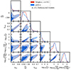 |
Fig. 6. Posterior distribution of the disfavoured values of the IGM parameters for the Ar = 0 scenario. These are disfavoured by the LOFAR upper limits from Mertens et al. (2025) at z = 9.1. Red refers to the case when z = 9.1 is considered separately (Single-z), while blue represents the joint redshift analysis obtained at z = 9.1 (Joint-z). The contour levels in the two-dimensional contour plots refer to the 1σ and 2σ credible intervals of the models disfavoured by the LOFAR upper limit at this redshift. The diagonal panels represent the corresponding marginalised probability distributions of each parameter. |
Table 4 also includes the results on the IGM parameters obtained from the MCMC analysis performed at the other two redshifts. The Single-z analysis gives fairly similar results at all redshifts, for both the 68% and 95% credible intervals levels. Indeed, the disfavoured IGM states are those which cause a high contrast in the δTb maps, producing large Δ2 values at scales 0.076 h Mpc−1 ≲ k ≲ 0.133 h Mpc−1. Unlike the Single-z case, in the Joint-z analysis the IGM parameter’s disfavoured credible intervals show a consistent evolution with redshift. For example, the 95% credible intervals limits on  are ≲0.85, ≲0.46 and ≲0.17 at z = 8.3, 9.1 and 10.1, respectively. The main reason behind this evolution is that in this case, the disfavoured limits of Mmin and Mmin, X are basically the same at all redshifts, while the number density of dark matter halos contributing to ionization or heating increases towards lower redshift for a fixed Mmin and Mmin, X. This causes a more efficient ionization and heating process towards the lower redshift for disfavoured models from the Joint-z analysis.
Constraints on the IGM parameters derived using the LOFAR upper limits from Mertens et al. (2025) for the Ar = 0 scenario.
3.2. Analysis with excess radio background (VaryingAr)
Next, we present the results of the MCMC analysis for the 5D source parameter space, i.e. ζ, Mmin, Mmin, X, fX and Ar, the same as above with the addition of the excess radio background. Table 2 lists the priors on these parameters.
Figure 7 shows the posterior distribution of the five parameters for the disfavoured models at z = 9.1. For the Single-z approach, the 68% disfavoured credible intervals limits are ζ ≲ 2.4,  ,
,  , fX ≲ 5.2 and Ar ≳ 4.6 (see Table 5). The 95% disfavoured credible intervals of the source parameters span the entire parameter ranges for all three Single-z and Joint-z analyses. The physical reasons behind the high amplitude of the large-scale power spectrum are the same as those discussed in the previous section. Additionally, a higher value of Ar increases the signal strength and thus the power spectrum amplitude. We note that the effect of Ar is model dependent. In fact, as for Ar = 0, also in this scenario the signal from fully ionized gas is zero because δTb = 0, while the strength of the signal from neutral or partially ionized gas increases for larger values of Ar. This causes a different enhancement in the power spectrum amplitude between a scenario with a large fraction of ionized regions (such as a patchy reionization scenario) and a neutral scenario (e.g. a patchy heating scenario with
  ). This is one of the major reasons behind the differences in the posterior distribution of the source parameters compared to the previous case.
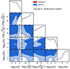 |
Fig. 7. Posterior distribution of the source parameters disfavoured values for the Varying Ar scenario. The corresponding models are disfavoured by the LOFAR upper limits from Mertens et al. (2025) at z = 9.1. Red refers to the case when each redshift is considered separately (Single-z) at z = 9.1, while blue represents the joint MCMC analysis results (Joint-z). The contour levels in the two-dimensional contour plots refer to the 1σ and 2σ credible intervals of the disfavoured models. The diagonal panels represent the corresponding marginalised probability distributions of each parameter. |
Constraints on the source parameters derived using the LOFAR upper limits from Mertens et al. (2025) for the Varying Ar scenario.
Table 5 shows the 68% credible intervals on the disfavoured values of the source parameters at all redshifts for the Single-z analysis, and at z = 9.1 for the Joint-z one. The credible intervals of the Single-z analysis are similar in trend for all redshifts, except for Mmin, X which remains unconstrained at z = 10.1. The disfavoured credible intervals on ζ and fX indicate smaller values towards lower redshifts. The 68% credible interval limits on disfavoured Ar values for the Single-z analysis correspond to Tγ, eff ≳ 60, 55 and 95 K at z = 8.3, 9.1 and 10.1, respectively, which are equivalent to an excess radio background larger than 140, 100, 207% of the CMB at 1.42 GHz. The Joint-z analysis posteriors for the source parameters show a trend similar to those from the Single-z cases, but closer to the z = 9.1 Single-z analysis results. The 68% credible intervals on the disfavoured Ar values correspond to Tγ, eff ≳ 43.2 K at z = 9.1 for the Joint-z analysis, meaning that an excess radio background higher than 57% of the CMB at 1.42 GHz is disfavoured. On the other hand, the 95% credible intervals on the disfavoured Ar value span the entire prior range of Ar for both the Single-z and Joint-z cases.
Figure 8 shows the IGM parameters’ posterior distributions for the disfavoured models obtained from the MCMC analysis at z = 9.1. The 68% (95%) credible intervals for the Single-z analysis case at z = 9.1 are  ,
,  K, fheat ≲ 0.05 (0.46),
  mK,
mK,  and
and  . The ionization and the thermal states of the disfavoured models are similar to those in the scenario with Ar = 0, and correspond to extreme models with rare and large ionized or heated regions. We repeat the caveat that the constraints on the IGM parameters might be significantly impacted by the chosen priors on the source parameters (see Appendix A for details).
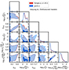 |
Fig. 8. Posterior distribution of the IGM parameters of the disfavoured models at z = 9.1 for the Varying Ar scenario. Red refers to the case when each redshift is considered separately (Single-z), while blue represents the joint MCMC analysis obtained at z = 9.1 (Joint-z). The contour levels in the two-dimensional contour plots refer to the 1σ and 2σ credible intervals of the models disfavoured by the LOFAR upper limit from Mertens et al. (2025) at this redshift. The diagonal panels represent the corresponding marginalised probability distributions of each parameter. |
Table 6 shows the disfavoured limits for all three Single-z and Joint-z analyses at 68% and 95% credible intervals. In the Single-z cases, the disfavoured limits on IGM parameters for all redshifts are similar, indicating that the IGM ionization and thermal states producing high amplitudes of the large-scale power spectra are similar. As in the case with Ar = 0, we also see a consistent redshift evolution of the IGM parameters’ disfavoured limits in the Joint-z analysis case.
Constraints on the IGM parameters derived using the LOFAR upper limits from Mertens et al. (2025) for the Varying Ar scenario.
3.3. Analysis including results from other interferometers
Besides LOFAR, several other radio interferometers, such as GMRT, PAPER, MWA and HERA, have produced upper-limits on the 21 cm signal power spectrum in the range z = 8 − 10. In this section we consider all available upper limits to derive constraints on the IGM physical properties in this redshift range. Except for LOFAR and MWA, the other upper limits are obtained in a limited small-scale range with k ≳ 0.3 h Mpc−1. Combining all available upper limits in a MCMC analysis needed to consider a broader k range compared to the earlier cases.
Figure 9 shows those 2σ upper limits along with 1000 GRIZZLY power spectra randomly chosen from the 105 simulations for Ar = 0. We note that at z ∼ 8 only LOFAR (Mertens et al. 2025) and HERA (Abdurashidova et al. 2023) upper limits can rule out some EoR models at the 2σ level. In comparison to LOFAR, a significantly larger number of models is ruled out by the HERA best 2σ upper limit Δ2(k = 0.34 h Mpc−1, z = 7.9, 1128 hours)≈(21.4)2 mK2, including the scenario of a completely neutral and unheated IGM (dashed line). This is consistent with the findings of Abdurashidova et al. (2022). The best upper limit from MWA (Trott et al. 2020), Δ2(k = 0.14 h Mpc−1, z = 7.8, 51 hours)≈(154)2 mK2, is still above the extreme EoR models power spectra by a factor of ≈2. The best 2σ result from PAPER is Δ2(k = 0.37 h Mpc−1, z = 8.4, 135 nights)≈(205)2 mK2, which is larger than the predicted power spectra by a factor of ≳4.
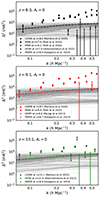 |
Fig. 9. Set of 1000 power spectra randomly chosen from the 105 simulated spectra for Ar = 0 scenario. Panels from top to bottom refer to z = 8.3, 9.1, and 10.1, respectively. The dashed lines correspond to the power spectrum for a completely neutral IGM with no X-ray heating and with TS = TK at those redshifts. The down arrow points refer to the different 2σ upper limits at those redshifts. |
At z ∼ 9, the LOFAR upper limits from Mertens et al. (2025) are the best available results, and remain the only ones which rule out a set of extreme EoR scenarios. The best 2σ upper limit from GMRT (Paciga et al. 2013) and MWA (Trott et al. 2020) at this redshift are Δ2(k = 0.5 h Mpc−1, z = 8.6, 50 hours)≈(248)2 mK2 and Δ2(k = 0.14 h Mpc−1, z = 8.8, 51 hours)≈(250)2 mK2, respectively, i.e. more than ≈6 times larger than our extreme models. The best 2σ result from PAPER is Δ2(k = 0.36 h Mpc−1, z = 8.7, 135 nights)≈(281)2 mK2, which is larger than the GRIZZLY power spectra by a factor of at least ≈8. We note that the neutral and unheated IGM scenario at z ∼ 9 (dashed curve) hasn’t been ruled out by any of these upper limits.
Similarly to z ∼ 8, also at z ∼ 10 only LOFAR and HERA upper limits can rule out some extreme EoR models, as shown in the bottom panel of Fig. 9. The best 2σ upper limit result from HERA at this redshift is Δ2(k = 0.36 h Mpc−1, z = 10.4, 1128 hours)≈(59)2 mK2, which is marginally able to rule out the neutral and unheated EoR scenario. Compared to z ∼ 8, the number of models ruled out by HERA at z ∼ 10 is smaller. The only other interferometer which has collected data at this redshift is PAPER, with a best 2σ result of Δ2(k = 0.34 h Mpc−1, z = 9.9, 135 nights)≈(1923)2 mK2, which is several orders of magnitude higher than our theoretical predictions.
Next, we performed an MCMC analysis on the disfavoured models for the Ar = 0 scenario, including all available upper limit results at z ∼ 8, 9, and 10. In this case, we included one k-bin corresponding to the best upper limit results from each telescope in addition to the three LOFAR k-bins considered in our previous analysis. We denote this as the allUL scenario. The 1D posterior distribution of the disfavoured source parameters for allUL and Ar = 0 is shown (dotted lines) in Fig. 10 along with the LOFAR only case (solid). The 68% disfavoured credible intervals from the Single-z analysis at z ∼ 9 for the allUL case are  and
and  , while the limits for ζ and fX span the entire parameter ranges. The 95% disfavoured credible intervals span the entire parameter ranges for both the Single-z and Joint-z analysis. For the Joint-z and
  analysis case, the 68% disfavoured credible intervals at z ∼ 9 are ζ ≲ 1.8 and
  , while the limits for Mmin, X and fX span the entire parameter ranges, similarly to the Single-z analysis. The presence of small-scale power spectra upper limits in the MCMC analysis, causes a significant change in the marginalised probability distribution of the source parameters with respect to the LOFAR-only case. The minimum change is observed at z ∼ 9, as the LOFAR upper limits at the large-scales are the best ones and thus dominate the MCMC analysis. Instead, at the other two redshifts the posteriors are mainly determined by the HERA upper limits.
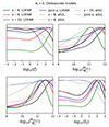 |
Fig. 10. Marginalised probability distribution of the disfavoured models’ source parameters at z ∼ 8, 9, and 10 for allUL case. The results are for the Ar = 0 scenario. The black, red, and green curves refer to the Single-z case at z = 8.3, 9.1 and 10.1, respectively, while the blue curves are for the Joint-z analysis case. The solid curves represent results derived from the LOFAR upper limits only, while the dotted curves refer to cases where we have used all available upper limits. |
In Fig. 11 we present the 1D marginalised probability distribution of the disfavoured models’ IGM parameters at z ∼ 9 for the allUL scenario with Ar = 0, which in the Single-z analysis case have  ,
,  K,
K,  mK,
mK,  and
and  at 68% (95%) credible intervals, while fheat spans the entire range. With the Joint-z analysis we instead obtain
  ,
,  K,
K,  mK, fheat ≲ 0.12(X),
  and
and  . While the constraints on
  look similar for the allUL and LOFAR-only cases, significant differences are seen for the other parameters. Indeed, due to the presence of the small-scale upper limits with a large error, more reionization scenarios with smaller emission/ionized regions are disfavoured in the allUL scenario.
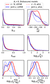 |
Fig. 11. Marginalised probability distribution of the IGM parameters of the disfavoured models at z ∼ 9 for allUL and Ar = 0 scenario. The red and blue curves refer to the Single-z and Joint-z cases, respectively. The solid curves represent results derived from the LOFAR upper limits only, while the dotted refer to cases where we have used all available upper limits. |
Finally, Fig. 12 presents the 1D marginalised probability distribution of the disfavoured IGM parameters at z ∼ 9 for the allUL and Varying Ar scenario. The 68% (95%) credible intervals of the disfavoured models for the Single-z analysis are  , fheat ≲ 0.06 (0.5)
  K,
K,  mK,
mK,  and
and  . For the Joint-z analysis, these intervals instead are
  ,
,  K,
K,  mK, fheat ≲ 0.12(X),
  and
and  . Table B2 presents the 68% and 95% credible intervals at all three redshifts for both the Single-z and Joint-z analysis. Contrary to Fig. 11, here we see that the constraints on all our IGM parameters look similar to the allUL and LOFAR-only case in the Single-z analysis. The difference on the posterior distributions for the Joint-z case as shown in Fig. 12 is also not as significant as found in Fig. 11. While the LOFAR z = 9.1 upper limits, being the best ones at this redshift, try to keep the MCMC results similar for the allUL and LOFAR-only Single-z case, the effect of source parameters’ priors in the Varying Ar scenario also play an important role in producing similar posterior distributions.
We have also performed an MCMC analysis for the other two redshifts, the results of which can be found in Appendix B. This includes the constraints on the IGM parameters for the allUL case in Tables B.1 and B2. Figures B.1 and B.2 show the comparison between the allUL and LOFAR-only Ar = 0 scenario for redshifts ∼ 8 and 10, respectively. Clearly, the 1D posterior distributions are biased by the HERA upper limits, making the allUL and LOFAR-only PDFs different for most of the IGM parameters. This is also true for Figs. B.3 and B.4, which show the same comparison but for the Varying Ar scenario for redshifts ∼ 8 and 10, respectively.
4. Summary and discussion
Recently, Mertens et al. (2025) analysed 140 hours of LOFAR data for redshifts 8.3, 9.1, and 10.1, and produced new upper limits on the dimensionless spherically averaged power spectrum of the 21 cm signal (see Table 1). Here, we have used those upper limits to infer the physical state of the IGM as well as the properties of the ionizing sources at those redshifts. As the upper limit results are still weak, we have derived constraints on the disfavoured rather than favoured models of reionization.
Our framework uses a databse of hundreds of thousands of reionization models simulated with the GRIZZLY code, which employs a one-dimensional radiative transfer approach. The models are obtained by changing the following parameters associated with source properties: ionization efficiency (ζ), minimum mass of the UV emitting halos (Mmin), minimum mass of X-ray emitting halos (Mmin, X), X-ray heating efficiency (fX), and the amplitude of a radio background in excess of the CMB (Ar). In addition to the power spectra of the 21 cm signal, various other quantities were derived from the reionization models to characterise the ionization and thermal state of the IGM, such as the volume-averaged ionization fraction ( ), volume-averaged gas temperature of the partially ionized IGM (
 ), mass-averaged brightness temperature (
 ), volume fraction of the heated region (fheat), size of the heated regions at which the PDF of the sizes peak (
 ), and FWHM of the PDFs (
 ). We then used an MCMC framework to derive constraints on the source parameters and IGM-related quantities. We considered two different scenarios, one in which there is no excess radio background and another in which there is one characterised by a parameter Ar. We performed one MCMC analysis considering each redshift independently (referred to as the Single-z analysis case) and another in which we derived a joint likelihood for the three redshifts (Joint-z analysis). The constraints obtained on the disfavoured source and IGM parameters are based on the chosen uniform priors of the source parameters as presented in Table 2. We highlight that our source parameters are assumed to be redshift independent, and thus the results of the Joint-z analysis should be interpreted with caution. The main findings of the paper can be summarised as follows.
-
More than 10% of the simulation database with Ar = 0 are well above Δ212(k, z)−Δ21, err2(k, z) in at least one k-bin at all three redshifts, indicating that these models have a high probability of being ruled out.
-
The models disfavoured by both the Single-z and the Joint-z analysis for the scenario with Ar = 0 typically have a small number density of bright UV and X-ray emitting sources at all redshifts. More specifically, in the Single-z analysis, the 68% credible intervals on the disfavoured Mmin and Mmin, X values at z = 9.1 are
 and
and  , respectively, while ζ and fX remain unconstrained (see Table 3 for the constraints at all redshifts). We find that the 95% disfavoured credible intervals of the source parameters span the entire prior ranges. The MCMC analysis results in the Joint-z case are significantly biased by the upper limits at z = 9.1, which are the strongest among the three redshifts considered here.
 -
For Ar = 0, the disfavoured limits on the IGM parameters at z = 9.1 are
 ,
,  K, fheat ≲ 0.18 (0.57),
  mK,
mK,  , and
, and  at the 68% (95%) credible interval level (see Table 4 for details), indicating extreme reionization models with rare and large ionized or heated regions. The Single-z analysis gives similar credible intervals at all redshifts, showing that only a few IGM physical states can produce very high amplitudes of the large-scale power spectrum. As for the source parameters, the results of the Joint-z analysis for the IGM parameters are mainly biased by the z = 9.1 upper limits. They show a consistent redshift evolution. For example, the 95% credible interval limits on
  are ≲0.85, ≲0.46, and ≲0.17 at z = 8.3, 9.1, and 10.1, respectively.
 -
When also considering an excess radio background, the models disfavoured by both the Single-z and the Joint-z analysis have a low number density of bright UV and X-ray emitting sources at all redshifts. More specifically, in the Single-z analysis, the 68% credible intervals on the source parameters at z = 9.1 are ζ ≲ 2.4,
 ,
,  , fX ≲ 5.2, and Ar ≳ 4.6 (see Table 5 for the constraints at all redshifts). We find that the 95% disfavoured credible intervals span the entire prior ranges of the source parameters for both the Single-z and Joint-z analysis. We also find that the 68% credible intervals are Ar ≳ 7.9 and 7.2 at z = 8.3 and 10.1, respectively, suggesting that an excess radio background that is at least 140%, 100%, and 207% of the CMB at 1.42 GHz is disfavoured at z = 8.3, 9.1, and 10.1, respectively. As for Ar = 0, the Joint-z analysis is biased by the upper limits at z = 9.1. In terms of the excess radio background, in this case we find that the 68% limits on the disfavoured models’ Ar at z = 9.1 correspond to an excess radio background that is ≳57% of the CMB at 1.42 GHz.
 -
For such a radio background model, the disfavoured limits on the IGM parameters are
 ,
,  K, fheat ≲ 0.05 (0.46),
  mK,
mK,  , and
, and  at z = 9.1 for the Single-z case at the 68% (95%) credible interval level (see Table 6 for all redshifts’ constraints). This indicates that the disfavoured ionization and thermal states are similar to those in the scenario with Ar = 0 and correspond to extreme reionization models with rare and large ionized or heated regions. Similarly to the Ar = 0 scenario, we also find a consistent redshift evolution of the IGM parameters’ disfavoured limits in the Joint-z analysis for the Varying Ar case.
 -
The inclusion of upper limits from other radio interferometric observations (allUL case) in our study significantly increases the disfavoured parameter space of both the source and IGM parameters. We find that the HERA upper limits dominate the Bayesian analysis at z ∼ 8 and 10, while the LOFAR ones prevail at z ∼ 9. The HERA upper limits rule out a neutral and unheated IGM at z ∼ 8 at a 2σ level. We find that the constraints on
 , and
, and  are similar for the allUL and LOFAR-only cases, while those on the other parameters are significantly different.
The constraints derived in this paper improve on those obtained in Ghara et al. (2020) using the earlier LOFAR upper limits at z = 9.1 from Mertens et al. (2020). Indeed, in the absence of a radio background in excess of the CMB, the 95% credible intervals on the disfavoured models’ IGM parameters obtained in Ghara et al. (2020) were fheat ≲ 0.34,  K,
K,  and
and  , while we found two regimes of disfavoured credible intervals for
  , i.e.
  and
and  . We note that there are some differences between the analysis done here and in Ghara et al. (2020). For example, the latter fixed Mmin = 109 M⊙ while varying ζ, Mmin, X and fX with different prior ranges, and they did not include redshift space distortions in their simulated power spectra, resulting in under-predictions of the large-scale power spectrum for several scenarios. The improvement in the present version of our interpretation framework, as well as in the observed upper limits, has enabled us to rule out more reionization models and produce better posterior distributions for both the disfavoured source and IGM parameters.
Previously, Mondal et al. (2020) constrained the excess radio background as 0.1–9.6% of the CMB at 1.42 GHz using the LOFAR upper limits at z = 9.1 from Mertens et al. (2020). We note that a direct comparison to these constraints is not possible, as they were obtained by marginalizing models that are allowed under those upper limits, while our results are derived from the marginalisation of the excluded models. In Ghara et al. (2021), an excess radio background of at least 25% of the CMB at 1.42 GHz was excluded using MWA upper limits in the range z = 6.5 − 8.7 from Trott et al. (2020) with 68% credible intervals on Ar.
The MCMC results presented in this study are dependent on the prior ranges of the source parameters. This is true not only for the disfavoured models but also for the allowed ones. Since the volume in parameter space is set by the priors, their impact can be very large, particularly if the interested scale is unknown and a flat prior in log space is employed. Therefore, the results strongly depend on the lower and upper limits set on the model parameters. In this work, we find that the constraints on  , fheat, and
  are significantly affected by the chosen priors on the source parameters (see Appendix A). To improve on this, observational data on high-z galactic properties, such as the luminosity function from the James Webb Space Telescope (JWST; e.g. Donnan et al. 2022; Castellano et al. 2023), can be used to increase our understanding of the prior ranges of the source parameters and thus to improve the constraints on the source and IGM parameters of the excluded models.
The upper limits on the 21 cm signal power spectrum used in this study contain excess noise and thus are conservative in nature. This is also applicable to the previous LOFAR upper limits from Patil et al. (2017), Mertens et al. (2020), and Ceccotti et al. (2025). The source of this excess noise is still uncertain (see e.g. Gan et al. 2022). Recently, Acharya et al. (2024c) considered applying a bias correction for excess noise as well, and they reported a 2σ upper limit of Δ2(k = 0.075 h Mpc−1, z = 9.1)≈(25)2 mK2 based on 141 hours of LOFAR data used in Mertens et al. (2020). In Appendix C, we perform an inference study on the Acharya et al. (2024c) upper limits and find that the 95% credible intervals of the IGM parameters of the allowed models are  ,
,  K, fheat ≳ 0.62,
  mK,
mK,  , and
, and  for the Varying Ar and Single-z scenario at z = 9.1. As in this scenario, the upper limits are stronger, and the results are on the allowed rather than the excluded models, so they cannot be directly compared to the results presented in the rest of the paper. We also caution the reader that the robustness of the Acharya et al. (2024c) upper limits needs further investigation, as also discussed in the original paper. For this reason, we have focused our attention on the constraints obtained from the weaker upper limits of Mertens et al. (2025).
We also note that in principle, an inference study such as the one discussed here should be included in the data analysis pipeline together with the foreground mitigation rather than as a separate step. This, however, is beyond the scope of this paper but will be considered in future studies.
It should be noted that the current LOFAR upper limits on Δ2 are rather large, and thus the constraints obtained on the disfavoured IGM and source parameters are not yet very strong. However, this study illustrates the potential of the 21 cm signal observation as a probe of the EoR, as even before an actual detection of the signal becomes available, more stringent upper limits on Δ2 would provide stronger constraints on the IGM parameters during the first billion years of the Universe. Additionally, other probes of this era such as the CMB, the global 21 cm signal, and high-z sources (e.g. galaxies, quasars, and fast radio bursts) will strengthen the understanding of the IGM during this crucial period in the Universe’s history. In particular, the detection of many faint galaxies at z ≳ 6 with JWST, complemented by observations with the Atacama Large Millimetre Array and the future European Extremely Large Telescope, will improve our understanding of the properties of early galaxies. This information will be fundamental to improving the prediction of the 21 cm signal through the calibration of the source model with these observations (see e.g. the GRIZZLY extension POLAR; Ma et al. 2023) and will thus provide a much deeper understanding of the EoR sources and IGM properties.
The initial strong upper limits from the PAPER collaboration (Beardsley et al. 2016) were later revised to a weaker upper bound after taking signal loss into account in their analysis (Cheng et al. 2018; Kolopanis et al. 2019).
Partnership for Advanced Computing in Europe: http://www.prace-ri.eu/
The amount of ionizing photons reaching the IGM depends on various quantities such as the star formation rate, the stellar initial mass function, the intrinsic ionizing photons emission rate, and the escape fraction. The parameter ζ combines the effects of all these.
The existence of a radio background of astrophysical or cosmological origin in addition to the CMB is motivated by the results of ARCADE2 (Fixsen et al. 2011) and LWA1 (Dowell & Taylor 2018) observations, which show evidence of excess towards the Rayleigh-Jeans part of the spectrum. In particular, the LWA1 measurement at frequency 40–80 MHz suggests a power-law dependence with spectral index –2.58 ± 0.05 and a temperature of  mK at 1.42 GHz. We note that the ARCADE2 and LWA1 measurements are debated, as the measurements might suffer from erroneous Galactic modelling (Subrahmanyan & Cowsik 2013).
We note that in our previous studies (Ghara et al. 2020, 2021) we ignored the redshift space distortions, which results in underestimating the 21 cm signal power spectrum, especially when it is dominated by density fluctuations.
Unlike in Ghara et al. (2020), here we do not consider separate probability distribution functions (PDFs) for the H II regions. In the absence of X-ray heating, the H II regions are equivalent to the heated regions, as the gas temperature within them is ∼104 K, i.e. much larger than Tγ, eff.
Each source parameter, si, is sampled by linearly binning the range [log10(si, min), log10(si, max)].
A comparison study of GRIZZLY with the 3D radiative transfer scheme C2RAY for different reionization scenarios assuming TS ≫ Tγ showed an excellent match of the power spectra, having a less than 10% difference (Ghara et al. 2018). However, the level of agreement across the entire parameter space is not known. Also, we do not have robust accuracy estimates of GRIZZLY for scenarios with TS fluctuations. Thus we used a conservative modelling error which also covers other uncertainties such as an interpolation error in the MCMC analysis. We note that the chosen modelling error is still significantly smaller than the 1σ error on the LOFAR upper limits at the large scales.
The exact redshift of the end of reionization (zend) is debated. While the Gunn-Peterson trough in high−z quasar spectra suggests zend ≈ 6 (e.g. Fan et al. 2006; Mortlock et al. 2011; Venemans et al. 2015; Bañados et al. 2018), Lyα forest observations at lower redshifts suggest a late reionization (see e.g. Becker et al. 2018; Eilers et al. 2018).
A credible interval is a parameter range with a certain probability (e.g. 68%) of containing the true value of the parameter. Our constraints on the source and IGM parameters do not represent models ruled out with a high significance, but rather models with a high probability to be excluded. These interval limits are also highly dependent on the prior chosen on the source parameter ranges.
Acknowledgments
RG acknowledges support from SERB, DST Ramanujan Fellowship no. RJF/2022/000141. We acknowledge that the N-body simulation used in this paper has been achieved using the PRACE Research Infrastructure resources Curie based at the Tr s Grand Centre de Calcul (TGCC) operated by CEA near Paris, France and Marenostrum based in the Barcelona Supercomputing Center, Spain (PRACE under PRACE4LOFAR grants 2012061089 and 2014102339 as well as under the Multi-scale Reionization grants 2014102281 and 2015122822). SKG is supported by NWO grant number OCENW.M.22.307. LVEK, SAB, KC, SG, CH and SM acknowledge the financial support from the European Research Council (ERC) under the European Union’s Horizon 2020 research and innovation programme (Grant agreement No. 884760, “CoDEX”). FGM acknowledges the support of the PSL Fellowship. EC acknowledge support from the Centre for Data Science and Systems Complexity (DSSC), Faculty of Science and Engineering at the University of Groningen, and the Ministry of Universities and Research (MUR) through the PRIN project ‘Optimal inference from radio images of the epoch of reionization’. SZ acknowledge support by the Israel Science Foundation (grant no. 1388/24). GM’s research is supported by the Swedish Research Council project grant 2020-04691_VR. MC’s research is supported by the Center for Fundamental Physics of the Universe(CFPU) Postdoctoral fellowship, Brown University, Providence, RI.
References
- Abdurashidova, Z., Aguirre, J. E., Alexander, P., et al. 2022, ApJ, 924, 51 [NASA ADS] [CrossRef] [Google Scholar]
- Abdurashidova, T. H. C. Z., Adams, T., Aguirre, J. E., et al. 2023, ApJ, 945, 124 [NASA ADS] [CrossRef] [Google Scholar]
- Acharya, S. K., Cyr, B., & Chluba, J. 2023, MNRAS, 523, 1908 [Google Scholar]
- Acharya, A., Mertens, F., Ciardi, B., et al. 2024a, MNRAS, 527, 7835 [Google Scholar]
- Acharya, A., Ma, Q. b., Giri, S. K., et al. 2024b, MNRAS, submitted [arXiv:2410.11620] [Google Scholar]
- Acharya, A., Mertens, F., Ciardi, B., et al. 2024c, MNRAS, 534, L30 [Google Scholar]
- Ali, Z. S., Parsons, A. R., Zheng, H., et al. 2015, ApJ, 809, 61 [NASA ADS] [CrossRef] [Google Scholar]
- Bañados, E., Venemans, B. P., Mazzucchelli, C., et al. 2018, Nature, 553, 473 [Google Scholar]
- Barkana, R. 2018, Nature, 555, 71 [Google Scholar]
- Barkana, R., & Loeb, A. 2001, Phys. Rep., 349, 125 [NASA ADS] [CrossRef] [Google Scholar]
- Barkana, R., & Loeb, A. 2005, ApJ, 626, 1 [Google Scholar]
- Barry, N., Hazelton, B., Sullivan, I., Morales, M. F., & Pober, J. C. 2016, MNRAS, 461, 3135 [CrossRef] [Google Scholar]
- Barry, N., Wilensky, M., Trott, C. M., et al. 2019, ApJ, 884, 1 [Google Scholar]
- Beardsley, A. P., Hazelton, B. J., Sullivan, I. S., et al. 2016, ApJ, 833, 102 [NASA ADS] [CrossRef] [Google Scholar]
- Becker, G. D., Bolton, J. S., Madau, P., et al. 2015, MNRAS, 447, 3402 [Google Scholar]
- Becker, G. D., Davies, F. B., Furlanetto, S. R., et al. 2018, ApJ, 863, 92 [NASA ADS] [CrossRef] [Google Scholar]
- Behroozi, P. S., & Silk, J. 2015, ApJ, 799, 32 [NASA ADS] [CrossRef] [Google Scholar]
- Bera, A., Ghara, R., Chatterjee, A., Datta, K. K., & Samui, S. 2023, JApA, 44, 10 [Google Scholar]
- Bernardi, G., Zwart, J. T. L., Price, D., et al. 2016, MNRAS, 461, 2847 [NASA ADS] [CrossRef] [Google Scholar]
- Bonaldi, A., & Brown, M. L. 2015, MNRAS, 447, 1973 [NASA ADS] [CrossRef] [Google Scholar]
- Bowman, J. D., & Rogers, A. E. E. 2010, Nature, 468, 796 [Google Scholar]
- Bowman, J. D., Rogers, A. E. E., Monsalve, R. A., Mozdzen, T. J., & Mahesh, N. 2018, Nature, 555, 67 [Google Scholar]
- Bradley, R. F., Tauscher, K., Rapetti, D., & Burns, J. O. 2019, ApJ, 874, 153 [NASA ADS] [CrossRef] [Google Scholar]
- Castellano, M., Fontana, A., Treu, T., et al. 2023, ApJ, 948, L14 [NASA ADS] [CrossRef] [Google Scholar]
- Ceccotti, E., Offringa, A. R., Koopmans, L. V. E., et al. 2025, A&A, 696, A56 [NASA ADS] [CrossRef] [EDP Sciences] [Google Scholar]
- Chapman, E., Zaroubi, S., Abdalla, F. B., et al. 2016, MNRAS, 458, 2928 [NASA ADS] [CrossRef] [Google Scholar]
- Chatterjee, A., Dayal, P., Choudhury, T. R., & Hutter, A. 2019, MNRAS, 487, 3560 [NASA ADS] [CrossRef] [Google Scholar]
- Chatterjee, A., Dayal, P., Choudhury, T. R., & Schneider, R. 2020, MNRAS, 496, 1445 [NASA ADS] [CrossRef] [Google Scholar]
- Cheng, C., Parsons, A. R., Kolopanis, M., et al. 2018, ApJ, 868, 26 [NASA ADS] [CrossRef] [Google Scholar]
- Choudhury, M., Ghara, R., Zaroubi, S., et al. 2024, arXiv e-prints [arXiv:2407.03523] [Google Scholar]
- Cohen, A., Fialkov, A., Barkana, R., & Monsalve, R. A. 2020, MNRAS, 495, 4845 [NASA ADS] [CrossRef] [Google Scholar]
- Cyr, B., Chluba, J., & Acharya, S. K. 2024, Phys. Rev. D, 109, L121301 [Google Scholar]
- Datta, K. K., Bharadwaj, S., & Choudhury, T. R. 2007, MNRAS, 382, 809 [NASA ADS] [CrossRef] [Google Scholar]
- Datta, A., Bowman, J. D., & Carilli, C. L. 2010, ApJ, 724, 526 [NASA ADS] [CrossRef] [Google Scholar]
- DeBoer, D. R., Parsons, A. R., Aguirre, J. E., et al. 2017, PASP, 129, 045001 [NASA ADS] [CrossRef] [Google Scholar]
- de Lera Acedo, E., de Villiers, D. I. L., Razavi-Ghods, N., et al. 2022, Nat. Astron., 6, 984 [NASA ADS] [CrossRef] [Google Scholar]
- Donnan, C. T., McLeod, D. J., Dunlop, J. S., et al. 2022, MNRAS, 518, 6011 [NASA ADS] [CrossRef] [Google Scholar]
- Dowell, J., & Taylor, G. B. 2018, ApJ, 858, L9 [Google Scholar]
- Draine, B. T., & Miralda-Escudé, J. 2018, ApJ, 858, L10 [Google Scholar]
- Eastwood, M. W., Anderson, M. M., Monroe, R. M., et al. 2019, AJ, 158, 84 [NASA ADS] [CrossRef] [Google Scholar]
- Edler, H. W., de Gasperin, F., & Rafferty, D. 2021, A&A, 652, A37 [NASA ADS] [CrossRef] [EDP Sciences] [Google Scholar]
- Eide, M. B., Ciardi, B., Graziani, L., et al. 2020, MNRAS, 498, 6083 [Google Scholar]
- Eilers, A.-C., Davies, F. B., & Hennawi, J. F. 2018, ApJ, 864, 53 [NASA ADS] [CrossRef] [Google Scholar]
- Ewall-Wice, A., Hewitt, J., Mesinger, A., et al. 2016, MNRAS, 458, 2710 [NASA ADS] [CrossRef] [Google Scholar]
- Ewall-Wice, A., Dillon, J. S., Liu, A., & Hewitt, J. 2017, MNRAS, 470, 1849 [CrossRef] [Google Scholar]
- Fan, X., Strauss, M. A., Becker, R. H., et al. 2006, AJ, 132, 117 [NASA ADS] [CrossRef] [Google Scholar]
- Fialkov, A., & Barkana, R. 2019, MNRAS, 486, 1763 [NASA ADS] [CrossRef] [Google Scholar]
- Fialkov, A., Barkana, R., & Cohen, A. 2018, Phys. Rev. Lett., 121, 011101 [NASA ADS] [CrossRef] [Google Scholar]
- Fixsen, D. J., Kogut, A., Levin, S., et al. 2011, ApJ, 734, 5 [Google Scholar]
- Furlanetto, S. R., Oh, S. P., & Briggs, F. H. 2006, Phys. Rep., 433, 181 [Google Scholar]
- Gan, H., Koopmans, L. V. E., Mertens, F. G., et al. 2022, A&A, 663, A9 [NASA ADS] [CrossRef] [EDP Sciences] [Google Scholar]
- Gan, H., Mertens, F. G., Koopmans, L. V. E., et al. 2023, A&A, 669, A20 [NASA ADS] [CrossRef] [EDP Sciences] [Google Scholar]
- Gao, L. Y., Koopmans, L. V. E., Mertens, F. G., et al. 2024, arXiv e-prints [arXiv:2412.16853] [Google Scholar]
- Gehlot, B. K., Mertens, F. G., Koopmans, L. V. E., et al. 2019, MNRAS, 488, 4271 [Google Scholar]
- Ghara, R., & Mellema, G. 2020, MNRAS, 492, 634 [NASA ADS] [CrossRef] [Google Scholar]
- Ghara, R., Choudhury, T. R., & Datta, K. K. 2015a, MNRAS, 447, 1806 [NASA ADS] [CrossRef] [Google Scholar]
- Ghara, R., Datta, K. K., & Choudhury, T. R. 2015b, MNRAS, 453, 3143 [Google Scholar]
- Ghara, R., Choudhury, T. R., & Datta, K. K. 2016, MNRAS, 460, 827 [NASA ADS] [CrossRef] [Google Scholar]
- Ghara, R., Choudhury, T. R., Datta, K. K., & Choudhuri, S. 2017, MNRAS, 464, 2234 [NASA ADS] [CrossRef] [Google Scholar]
- Ghara, R., Mellema, G., Giri, S. K., et al. 2018, MNRAS, 476, 1741 [NASA ADS] [CrossRef] [Google Scholar]
- Ghara, R., Giri, S. K., Mellema, G., et al. 2020, MNRAS, 493, 4728 [NASA ADS] [CrossRef] [Google Scholar]
- Ghara, R., Giri, S. K., Ciardi, B., Mellema, G., & Zaroubi, S. 2021, MNRAS, 503, 4551 [NASA ADS] [CrossRef] [Google Scholar]
- Ghara, R., Mellema, G., & Zaroubi, S. 2022, JCAP, 2022, 055 [CrossRef] [Google Scholar]
- Ghara, R., Shaw, A. K., Zaroubi, S., et al. 2024, A&A, 687, A252 [NASA ADS] [CrossRef] [EDP Sciences] [Google Scholar]
- Ghosh, A., Prasad, J., Bharadwaj, S., Ali, S. S., & Chengalur, J. N. 2012, MNRAS, 426, 3295 [NASA ADS] [CrossRef] [Google Scholar]
- Giri, S. K., Mellema, G., Aldheimer, T., Dixon, K. L., & Iliev, I. T. 2019a, MNRAS, 489, 1590 [NASA ADS] [CrossRef] [Google Scholar]
- Giri, S. K., D’Aloisio, A., Mellema, G., et al. 2019b, JCAP, 2019, 058 [Google Scholar]
- Greig, B., Mesinger, A., Koopmans, L. V. E., et al. 2021, MNRAS, 501, 1 [Google Scholar]
- Harker, G., Zaroubi, S., Bernardi, G., et al. 2009, MNRAS, 397, 1138 [NASA ADS] [CrossRef] [Google Scholar]
- Harnois-Déraps, J., Pen, U.-L., Iliev, I. T., et al. 2013, MNRAS, 436, 540 [Google Scholar]
- Hills, R., Kulkarni, G., Meerburg, P. D., & Puchwein, E. 2018, Nature, 564, E32 [Google Scholar]
- Hinshaw, G., Larson, D., Komatsu, E., et al. 2013, ApJS, 208, 19 [Google Scholar]
- Hothi, I., Chapman, E., Pritchard, J. R., et al. 2021, MNRAS, 500, 2264 [Google Scholar]
- Hu, E. M., Cowie, L. L., Barger, A. J., et al. 2010, ApJ, 725, 394 [Google Scholar]
- Islam, N., Ghara, R., Paul, B., Choudhury, T. R., & Nath, B. B. 2019, MNRAS, 487, 2785 [NASA ADS] [CrossRef] [Google Scholar]
- Jelić, V., Zaroubi, S., Labropoulos, P., et al. 2010, MNRAS, 409, 1647 [CrossRef] [Google Scholar]
- Kern, N. S., Parsons, A. R., Dillon, J. S., et al. 2019, ApJ, 884, 105 [NASA ADS] [CrossRef] [Google Scholar]
- Kern, N. S., Parsons, A. R., Dillon, J. S., et al. 2020, ApJ, 888, 70 [NASA ADS] [CrossRef] [Google Scholar]
- Kolopanis, M., Jacobs, D. C., Cheng, C., et al. 2019, ApJ, 883, 133 [NASA ADS] [CrossRef] [Google Scholar]
- Koopmans, L., Pritchard, J., Mellema, G., et al. 2015, Proceedings of Advancing Astrophysics with the Square Kilometre Array – PoS(AASKA14), AASKA14 (Sissa Medialab) [Google Scholar]
- Krause, F., Thomas, R. M., Zaroubi, S., & Abdalla, F. B. 2018, New Astron., 64, 9 [NASA ADS] [CrossRef] [Google Scholar]
- Lewis, A., & Bridle, S. 2002, Phys. Rev. D, 66, 103511 [Google Scholar]
- Liu, A., Parsons, A. R., & Trott, C. M. 2014, Phys. Rev. D, 90, 023019 [NASA ADS] [CrossRef] [Google Scholar]
- Ma, Q.-B., Ghara, R., Ciardi, B., et al. 2023, MNRAS, 522, 3284 [NASA ADS] [CrossRef] [Google Scholar]
- Madau, P., Meiksin, A., & Rees, M. J. 1997, ApJ, 475, 429 [NASA ADS] [CrossRef] [Google Scholar]
- Mao, Y., Shapiro, P. R., Mellema, G., et al. 2012, MNRAS, 422, 926 [NASA ADS] [CrossRef] [Google Scholar]
- Mellema, G., Koopmans, L. V. E., Abdalla, F. A., et al. 2013, Exp. Astron., 36, 235 [NASA ADS] [CrossRef] [Google Scholar]
- Mellema, G., Koopmans, L., Shukla, H., et al. 2015, Advancing Astrophysics with the Square Kilometre Array (AASKA14) , 10 [Google Scholar]
- Mertens, F. G., Ghosh, A., & Koopmans, L. V. E. 2018, MNRAS, 478, 3640 [NASA ADS] [Google Scholar]
- Mertens, F. G., Mevius, M., Koopmans, L. V. E., et al. 2020, MNRAS, 493, 1662 [Google Scholar]
- Mertens, F. G., Bobin, J., & Carucci, I. P. 2024, MNRAS, 527, 3517 [Google Scholar]
- Mertens, F. G., Mevius, M., Koopmans, L. V. E., et al. 2025, A&A, 698, A186 [NASA ADS] [CrossRef] [EDP Sciences] [Google Scholar]
- Mesinger, A., & Furlanetto, S. 2007, ApJ, 669, 663 [Google Scholar]
- Mevius, M., van der Tol, S., Pandey, V. N., et al. 2016, Radio Sci., 51, 927 [Google Scholar]
- Mevius, M., Mertens, F., Koopmans, L. V. E., et al. 2022, MNRAS, 509, 3693 [Google Scholar]
- Mineo, S., Gilfanov, M., & Sunyaev, R. 2012, MNRAS, 419, 2095 [Google Scholar]
- Mirocha, J., Muñoz, J. B., Furlanetto, S. R., Liu, A., & Mesinger, A. 2022, MNRAS, 514, 2010 [NASA ADS] [CrossRef] [Google Scholar]
- Mondal, R., Fialkov, A., Fling, C., et al. 2020, MNRAS, 498, 4178 [NASA ADS] [CrossRef] [Google Scholar]
- Monsalve, R. A., Rogers, A. E. E., Bowman, J. D., & Mozdzen, T. J. 2017, ApJ, 835, 49 [Google Scholar]
- Monsalve, R. A., Fialkov, A., Bowman, J. D., et al. 2019, ApJ, 875, 67 [NASA ADS] [CrossRef] [Google Scholar]
- Monsalve, R. A., Altamirano, C., Bidula, V., et al. 2024, MNRAS, 530, 4125 [Google Scholar]
- Morales, A. M., Mason, C. A., Bruton, S., et al. 2021, ApJ, 919, 120 [CrossRef] [Google Scholar]
- Mortlock, D. J., Warren, S. J., Venemans, B. P., et al. 2011, Nature, 474, 616 [Google Scholar]
- Muñoz, J. B., & Loeb, A. 2018, Nature, 557, 684 [Google Scholar]
- Munshi, S., Mertens, F. G., Koopmans, L. V. E., et al. 2024, A&A, 681, A62 [NASA ADS] [CrossRef] [EDP Sciences] [Google Scholar]
- Munshi, S., Mertens, F. G., Koopmans, L. V. E., et al. 2025, A&A, 697, A203 [NASA ADS] [CrossRef] [EDP Sciences] [Google Scholar]
- Nebrin, O., Ghara, R., & Mellema, G. 2019, JCAP, 2019, 051 [CrossRef] [Google Scholar]
- Offringa, A. R., Mertens, F., & Koopmans, L. V. E. 2019, MNRAS, 484, 2866 [CrossRef] [Google Scholar]
- Paciga, G., Albert, J. G., Bandura, K., et al. 2013, MNRAS, 433, 639 [CrossRef] [Google Scholar]
- Park, J., Mesinger, A., Greig, B., & Gillet, N. 2019, MNRAS, 484, 933 [NASA ADS] [CrossRef] [Google Scholar]
- Parsons, A. R., Liu, A., Aguirre, J. E., et al. 2014, ApJ, 788, 106 [NASA ADS] [CrossRef] [Google Scholar]
- Patil, A. H., Yatawatta, S., Zaroubi, S., et al. 2016, MNRAS, 463, 4317 [NASA ADS] [CrossRef] [Google Scholar]
- Patil, A. H., Yatawatta, S., Koopmans, L. V. E., et al. 2017, ApJ, 838, 65 [NASA ADS] [CrossRef] [Google Scholar]
- Patra, N., Subrahmanyan, R., Sethi, S., Udaya Shankar, N., & Raghunathan, A. 2015, ApJ, 801, 138 [NASA ADS] [CrossRef] [Google Scholar]
- Philip, L., Abdurashidova, Z., Chiang, H. C., et al. 2018, J. Astron. Instrum., submitted [arXiv:1806.09531] [Google Scholar]
- Planck Collaboration VI. 2020, A&A, 641, A6 [NASA ADS] [CrossRef] [EDP Sciences] [Google Scholar]
- Price, D. C., Greenhill, L. J., Fialkov, A., et al. 2018, MNRAS, 478, 4193 [NASA ADS] [Google Scholar]
- Pritchard, J. R., & Loeb, A. 2012, Rep. Progr. Phys., 75, 086901 [CrossRef] [Google Scholar]
- Reis, I., Fialkov, A., & Barkana, R. 2020, MNRAS, 499, 5993 [CrossRef] [Google Scholar]
- Ross, H. E., Dixon, K. L., Ghara, R., Iliev, I. T., & Mellema, G. 2019, MNRAS, 487, 1101 [NASA ADS] [CrossRef] [Google Scholar]
- Ross, H. E., Giri, S. K., Mellema, G., et al. 2021, MNRAS, 506, 3717 [NASA ADS] [CrossRef] [Google Scholar]
- Schaeffer, T., Giri, S. K., & Schneider, A. 2024, Phys. Rev. D, 110, 023543 [Google Scholar]
- Schneider, A., Giri, S. K., & Mirocha, J. 2021, Phys. Rev. D, 103, 083025 [NASA ADS] [CrossRef] [Google Scholar]
- Shapiro, P. R., Giroux, M. L., & Babul, A. 1994, ApJ, 427, 25 [Google Scholar]
- Singh, S., & Subrahmanyan, R. 2019, ApJ, 880, 26 [Google Scholar]
- Singh, S., Subrahmanyan, R., Udaya Shankar, N., et al. 2017, ApJ, 845, L12 [NASA ADS] [CrossRef] [Google Scholar]
- Singh, S., Jishnu, N. T., Subrahmanyan, R., et al. 2022, Nat. Astron., 6, 607 [NASA ADS] [CrossRef] [Google Scholar]
- Sobacchi, E., & Mesinger, A. 2013, MNRAS, 432, L51 [NASA ADS] [CrossRef] [Google Scholar]
- Sokolowski, M., Tremblay, S. E., Wayth, R. B., et al. 2015, PASA, 32, e004 [Google Scholar]
- Spinelli, M., Bernardi, G., & Santos, M. G. 2018, MNRAS, 479, 275 [Google Scholar]
- Springel, V., & Hernquist, L. 2003, MNRAS, 339, 312 [NASA ADS] [CrossRef] [Google Scholar]
- Subrahmanyan, R., & Cowsik, R. 2013, ApJ, 776, 42 [Google Scholar]
- Sun, G., & Furlanetto, S. R. 2016, MNRAS, 460, 417 [CrossRef] [Google Scholar]
- Tang, M., Stark, D. P., Chen, Z., et al. 2023, MNRAS, 526, 1657 [NASA ADS] [CrossRef] [Google Scholar]
- Thomas, R. M., & Zaroubi, S. 2008, MNRAS, 384, 1080 [Google Scholar]
- Thomas, R. M., & Zaroubi, S. 2011, MNRAS, 410, 1377 [NASA ADS] [CrossRef] [Google Scholar]
- Thomas, R. M., Zaroubi, S., Ciardi, B., et al. 2009, MNRAS, 393, 32 [Google Scholar]
- Tingay, S. J., Goeke, R., Bowman, J. D., et al. 2013, PASA, 30, 7 [Google Scholar]
- Trott, C. M., Jordan, C. H., Midgley, S., et al. 2020, MNRAS, 493, 4711 [NASA ADS] [CrossRef] [Google Scholar]
- van Haarlem, M. P., Wise, M. W., Gunst, A. W., et al. 2013, A&A, 556, A2 [NASA ADS] [CrossRef] [EDP Sciences] [Google Scholar]
- Venemans, B. P., Bañados, E., Decarli, R., et al. 2015, ApJ, 801, L11 [Google Scholar]
- Virtanen, P., Gommers, R., Oliphant, T. E., et al. 2020, Nat. Methods, 17, 261 [Google Scholar]
- Voytek, T. C., Natarajan, A., Jáuregui García, J. M., Peterson, J. B., & López-Cruz, O. 2014, ApJ, 782, L9 [Google Scholar]
- Watson, W. A., Iliev, I. T., D’Aloisio, A., et al. 2013, MNRAS, 433, 1230 [Google Scholar]
- Weiser, A., & Zarantonello, S. E. 1988, Math. Comput., 50, 189 [Google Scholar]
- Wilensky, M. J., Morales, M. F., Hazelton, B. J., et al. 2019, PASP, 131, 114507 [NASA ADS] [CrossRef] [Google Scholar]
- Witten, C., Laporte, N., Martin-Alvarez, S., et al. 2024, Nat. Astron., 8, 384 [Google Scholar]
- Yatawatta, S., & Banerjee, P. 2011, 2011 XXXth URSI General Assembly and Scientific Symposium (IEEE Piscataway) [Google Scholar]
- Zaroubi, S. 2013, in The First Galaxies, eds. T. Wiklind, B. Mobasher, & V. Bromm, Astrophysics and Space Science Library, 396, 45 [NASA ADS] [CrossRef] [Google Scholar]
Appendix A: Effect of the source parameter priors on the IGM parameters constraints
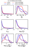 |
Fig. A.1. Marginalised probability distribution of the IGM parameters of the disfavoured models for a constant exclusion likelihood. The red and blue curves refer to the Single-z and Joint-z cases at z = 9.1, respectively. The solid curves represent results from the main text, while the dashed refers to cases where we have used ℒex, single − z(θ, z = 9.1) = 0.5 and ℒex, joint − z(θ, z = 9.1) = 0.5. |
In the study described in the main text we use source parameters as input for the MCMC analysis. After this the list of source parameter values is used to produce a corresponding list of IGM parameters, which is then employed to constrain the IGM parameters themselves. This method might introduce non-uniform posterior distributions of the IGM parameters even when the LOFAR upper limits are not considered in the analysis. In this section, we aim to investigate the effect of the source parameters’ priors on the constraints on the IGM parameters, by adopting the following approach. We fix to 0.5 the exclusion likelihood shown in Eqs. (3) and (4), independently from the LOFAR upper limits, but still use the priors on the maximum value of  , and we denote this as the no-LOFAR scenario. In this case, the posterior distribution of the source parameters is expected to be independent of the choice of the constant likelihood, while the posterior distribution of the disfavoured IGM parameter values is entirely determined by the chosen priors on the source parameters.
We consider the four source parameters for the Ar = 0 scenario from Sect. 3.1, but with a constant likelihood. The dashed curves in Fig. A.1 refer to the resulting marginalised probability distribution of the IGM parameters of the disfavoured models, for both the Single-z and Joint-z analysis. The distribution shows the effect of the source priors on the posteriors for the IGM parameters. The disfavoured models have  ,
,  K, no constraints on fheat,
  mK,
mK,  and
and  at 68% (95%) credible intervals for the Single-zno-LOFAR analysis case. For the Joint-zno-LOFAR analysis case, the disfavoured models’ 68% (95%) credible intervals are
  ,
,  K, no constraints on fheat,
  mK,
mK,  and
and  . For comparison, the solid curves show the probability distribution of the IGM parameters of the disfavoured models obtained in Section 3.1. Any differences between the solid and dashed curves are due to the effect of using the LOFAR upper limits. Such differences are clearly visible for
  ,
,  and
and  , they are less prominent for
  , fheat and
  . This suggests that the LOFAR upper limits provide very weak constraints on the latter three IGM parameters. The fact that the posterior for
  is affected by the LOFAR upper limits but the other averages (
 , fheat and
  ) are not, suggests that the correlations between δ, xHII and TK play important roles in determining the 21 cm signal power spectra (see e.g. Schaeffer et al. 2024).
Appendix B: Inference including all available upper limit results at z ∼ 8 and 10
While the results from the MCMC analysis which includes all available upper limits (allUL case) at z ∼ 9 have been discussed in Sect. 3.3, here we present the results at z ∼ 8 and 10. The 68% disfavoured credible intervals of the source parameters for the Ar = 0 and Single-z scenario at z ∼ 8 are ζ ≲ 1.6 and  , while the limits for Mmin, X and fX span the entire parameter ranges (see Fig. 10). The same intervals for z ∼ 10 are ζ ≲ 5,
 ,
,  , and fX ≲ 4. In this case, the source parameters’ 95% disfavoured credible intervals span the entire parameter ranges for both the redshifts. The 1D marginalised probability distribution of the source parameters at z ∼ 8 and 10 for the
  case are significantly different from the LOFAR-only case, as HERA upper limits dominate the MCMC analysis at these two redshifts.
Constraints on the IGM parameters for the Ar = 0 and allUL scenario for both the Single-z and Joint-z analysis at three redshifts.
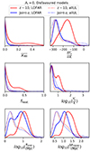 |
Fig. B.2. Marginalised probability distribution of the disfavoured models’ IGM parameters at z ∼ 10 for the allUL and Ar = 0 scenario. The red and blue curves refer to the Single-z and Joint-z cases, respectively. The solid curves represent results when we consider LOFAR upper limits only, while the dotted curves refer to cases where we have used all available upper limit results from different radio interferometric observations. |
The 1D marginalised probability distribution of the disfavoured IGM parameters for the Ar = 0 and allUL case at z ∼ 8 are shown in Fig. B.1 while Fig. B.2 shows the same but for z ∼ 10. The disfavoured models at z ∼ 8 in the allUL, Single-z and Ar = 0 scenario have  ,
,  K,
K,  mK,
mK,  and
and  , while fheat spans the entire range at 68% (95%) credible intervals. The disfavoured models at z ∼ 10 in the allULSingle-z case have
  ,
,  K,
K,  mK, fheat ≲ 0.03(0.36)
  and
and  at 68% (95%) credible intervals. As expected, the disfavoured IGM parameter space is much larger in the allUL case compared to the LOFAR-only case at z ∼ 8 and 10, as the MCMC analysis is mainly driven by the strong HERA upper limits. The 68% and 95% credible intervals for the Joint-zallUL case are shown in Table B.1. The numbers show that the results for the Joint-z MCMC analysis are mainly driven by the HERA upper limits at z ∼ 8.
Next we consider the Varying Ar scenario, starting with the Single-z and  case. In this case, the disfavoured models at z ∼ 8 show 68% credible intervals on the source parameters as ζ ≲ 1.7,
 , while the credible intervals of other parameters span the entire range. The same intervals for z ∼ 10 are ζ ≲ 3.3,
 and fX ≲ 5.5, while the other two parameters’ credible intervals span the entire ranges. The 1D marginalised probability distribution of the disfavoured IGM parameters for this case at z ∼ 8 and 10 is shown in Fig. B.3 and B.4, respectively. The disfavoured models at z ∼ 8 have
  ,
,  K,
K,  mK,
mK,  and
and  , while fheat spans the entire range at 68% (95%) credible intervals for the Single-z analysis case. The disfavoured models at z ∼ 10 in the allUL and Varying Ar
case have
, while fheat spans the entire range at 68% (95%) credible intervals for the Single-z analysis case. The disfavoured models at z ∼ 10 in the allUL and Varying Ar
case have  ,
,  K,
K,  mK, fheat ≲ 0.03(0.31)
  and
and  at 68% (95%) credible intervals for the Single-z analysis case.
The 68%and 95% credible intervals for the Joint-z, allUL case under the Varying Ar scenario are shown in Table B2. Similarly to the Ar = 0 scenario above, we find that the Joint-z MCMC analysis is also mostly driven by HERA upper limits at z ∼ 8.
Constraints on the IGM parameters at three different redshifts for the Varying Ar and allUL scenario for both the Single-z and Joint-z analysis.
Appendix C: Inference using Acharya et al. (2024c) upper limit results
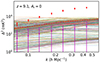 |
Fig. C.1. A subset of 1000 power spectra simulated with GRIZZLY at z = 9.1. These power spectra correspond to those with Ar = 0. The red and magenta points refer to the recent LOFAR 1σ upper limits from Mertens et al. (2025) and Acharya et al. (2024c), respectively. As a reference, the red dashed line corresponds to the power spectrum for a completely neutral IGM with no X-ray heating and TS = TK. |
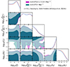 |
Fig. C.2. Posterior distribution of the source parameters at z = 9.1 for the Varying Ar scenario. These models are favoured by the LOFAR upper limits from Acharya et al. (2024c). Magenta indicates the case in which upper limits in three k−bins are considered, while teal represents the case when only one k−bin is used. The contour levels in the two-dimensional contour plots refer to the 1σ and 2σ credible intervals of the models favoured by the LOFAR upper limit at this redshift. The diagonal panels represent the corresponding marginalised probability distributions of each parameter. |
The LOFAR upper limits considered in the main text, as well as those obtained by Mertens et al. (2020), contain excess noise and thus are conservative limits in nature. Recently, Acharya et al. (2024c) have re-analysed the 10 nights of data used in Mertens et al. (2020) with a different approach, and reported a much stronger 2σ upper limit of  (see Table C1). This was obtained by assuming an accurate bias correction for the excess noise by subtracting the excess component. As this approach increases the risk of signal loss, more testing is required to verify the robustness of the results. Nevertheless, here we use these upper limits to explore their impact on the derived constraints for the physical state of the IGM.
Upper limit on Δ2 as reported in Acharya et al. (2024c) at z = 9.1 for different k-bins.
Figure C.1 shows 1000 randomly chosen models from the GRIZZLY simulation database, together with the LOFAR 1σ upper limits from Mertens et al. (2025, red) and Acharya et al. (2024c, magenta, Δ21 − an2 with error Δ21 − an, err2). We see that the red dashed curve, corresponding to the power spectrum of a completely neutral and unheated IGM at z = 9.1 obtained assuming constant values of xHI = 1 and TS = TK = 2 K, remains above the 1σ upper limits from Acharya et al. (2024c) at least for one k−bin. Unlike the results presented in the main text, here we find that all models are above Δ21 − an2 − Δ21 − an, err2.
When performing the same MCMC analysis discussed in the main text to identify the disfavoured models, we find that the marginalised probabilities are high over the full parameter space, indicating that a large number of models are disfavoured. For this reason, differently from the analysis performed in the main text, here we choose to study the properties of the favoured models by adopting for the likelihood of a model surviving at z the expression ℒsu, single − z(θ, z) = 1 − ℒex, single − z(θ, z).
We perform the Single-z analysis following two approaches, the first of which is the same one adopted in the main text, i.e. we consider the upper limits at the three smallest k−bins. In the second case, instead, we consider only the smallest k−bin upper limit, which is the strongest, and thus it is the one that mainly affects the constraints on the source and IGM parameters. Using only one k−bin also have the advantage of breaking the correlation originating from the approach adopted in Acharya et al. (2024c) when using upper limits at different k−bins.
Figure C.2 shows the posterior distribution of the source parameters for the Varying Ar scenario at z = 9.1 obtained from the MCMC analysis using the upper limits from Acharya et al. (2024c) on the allowed models. The 68% credible intervals limits of the allowed models are ζ ≲ 14,  ,
,  , fX ≳ 100 and Ar ≲ 2 for the Varying Ar scenario. The limits are similar when we use one upper limit at k = 0.075 h Mpc−1.
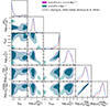 |
Fig. C.3. Posterior distribution of the IGM parameters at z = 9.1 for the Varying Ar scenario. These posterior distributions correspond to the models that are favoured by the LOFAR upper limits from Acharya et al. (2024c). Magenta indicates the case in which upper limits in three k−bins are considered, while teal represents the case when only one k−bin is used. The contour levels in the two-dimensional contour plots refer to the 1σ and 2σ credible intervals of the models favoured by the LOFAR upper limits at this redshift. The diagonal panels represent the corresponding marginalised probability distributions of each parameter. |
Figure C.3 shows the posterior distribution of the IGM parameters of the favoured models obtained from the Single-z analysis with the upper limits from Acharya et al. (2024c) at z = 9.1. The 95% credible intervals of the allowed models’ IGM parameters are  ,
,  K, fheat ≳ 0.62,
  mK,
mK,  and
and  . The limits on the IGM parameters for the case where we used the upper limit at k = 0.075 h Mpc−1 only are similar to the case where we used three k−bins upper limits. We note that, similar to the scenarios considered in the main text, these constraints are also highly dependent on the chosen priors on the source parameters (see Appendix A).
All Tables
Constraints on the source parameters derived using the LOFAR upper limits from Mertens et al. (2025) for the Ar = 0 scenario.
Constraints on the IGM parameters derived using the LOFAR upper limits from Mertens et al. (2025) for the Ar = 0 scenario.
Constraints on the source parameters derived using the LOFAR upper limits from Mertens et al. (2025) for the Varying Ar scenario.
Constraints on the IGM parameters derived using the LOFAR upper limits from Mertens et al. (2025) for the Varying Ar scenario.
Constraints on the IGM parameters for the Ar = 0 and allUL scenario for both the Single-z and Joint-z analysis at three redshifts.
Constraints on the IGM parameters at three different redshifts for the Varying Ar and allUL scenario for both the Single-z and Joint-z analysis.
Upper limit on Δ2 as reported in Acharya et al. (2024c) at z = 9.1 for different k-bins.
All Figures
|
Fig. 1. Set of 1000 power spectra randomly chosen from the 105 simulated power spectra. Panels from top to bottom refer to z = 8.3, 9.1, and 10.1, respectively. These correspond to the scenario with no additional radio background other than the CMB (Ar = 0). The down arrow points refer to the recent LOFAR 1σ upper limit (Δ212(k, z)±Δ21, err2(k, z)) from Mertens et al. (2025). As a reference, the dashed line corresponds to the power spectrum for a completely neutral IGM with no X-ray heating, and with TS = TK. The coloured power spectra are those with a value larger than Δ212(k, z)−Δ21, err2(k, z) in at least one k-bin, i.e. they have a high probability of being ruled out, while those in grey have a low exclusion probability. |
| In the text | |
|
Fig. 2. Histogram of the disfavoured values of the source parameters for the scenario with Ar = 0. These correspond to the models with power spectra values larger than Δ212(k, z)−Δ21, err2(k, z) in at least one k-bin, and they have a high probability of being ruled out by the recent LOFAR 1σ upper limits (Δ212(k, z)±Δ21, err2(k, z)) from Mertens et al. (2025). |
| In the text | |
|
Fig. 3. Histogram of the disfavoured values of the IGM parameters for the scenario with Ar = 0. These correspond to the same set of models considered in Fig. 2. |
| In the text | |
|
Fig. 4. Posterior distribution of the disfavoured values of the source parameters for the Ar = 0 scenario. These are disfavoured by the LOFAR upper limits from Mertens et al. (2025) at z = 9.1. Red refers to the case when each redshift is considered separately (Single-z) at z = 9.1, while blue represents the joint MCMC analysis results (Joint-z). The contour levels in the two-dimensional contour plots refer to the 1σ and 2σ credible intervals of the models disfavoured by the LOFAR upper limit at this redshift. The diagonal panels represent the corresponding marginalised probability distributions of each parameter. |
| In the text | |
|
Fig. 5. Marginalised probability distribution of the disfavoured values of the source parameters for the Ar = 0 scenario. The corresponding models are disfavoured by the LOFAR upper limits from Mertens et al. (2025) at z = 9.1. The black, red, and green curves refer to the Single-z case at z = 8.3, 9.1 and 10.1, respectively, while the blue curves are for the Joint-z analysis case. |
| In the text | |
|
Fig. 6. Posterior distribution of the disfavoured values of the IGM parameters for the Ar = 0 scenario. These are disfavoured by the LOFAR upper limits from Mertens et al. (2025) at z = 9.1. Red refers to the case when z = 9.1 is considered separately (Single-z), while blue represents the joint redshift analysis obtained at z = 9.1 (Joint-z). The contour levels in the two-dimensional contour plots refer to the 1σ and 2σ credible intervals of the models disfavoured by the LOFAR upper limit at this redshift. The diagonal panels represent the corresponding marginalised probability distributions of each parameter. |
| In the text | |
|
Fig. 7. Posterior distribution of the source parameters disfavoured values for the Varying Ar scenario. The corresponding models are disfavoured by the LOFAR upper limits from Mertens et al. (2025) at z = 9.1. Red refers to the case when each redshift is considered separately (Single-z) at z = 9.1, while blue represents the joint MCMC analysis results (Joint-z). The contour levels in the two-dimensional contour plots refer to the 1σ and 2σ credible intervals of the disfavoured models. The diagonal panels represent the corresponding marginalised probability distributions of each parameter. |
| In the text | |
|
Fig. 8. Posterior distribution of the IGM parameters of the disfavoured models at z = 9.1 for the Varying Ar scenario. Red refers to the case when each redshift is considered separately (Single-z), while blue represents the joint MCMC analysis obtained at z = 9.1 (Joint-z). The contour levels in the two-dimensional contour plots refer to the 1σ and 2σ credible intervals of the models disfavoured by the LOFAR upper limit from Mertens et al. (2025) at this redshift. The diagonal panels represent the corresponding marginalised probability distributions of each parameter. |
| In the text | |
|
Fig. 9. Set of 1000 power spectra randomly chosen from the 105 simulated spectra for Ar = 0 scenario. Panels from top to bottom refer to z = 8.3, 9.1, and 10.1, respectively. The dashed lines correspond to the power spectrum for a completely neutral IGM with no X-ray heating and with TS = TK at those redshifts. The down arrow points refer to the different 2σ upper limits at those redshifts. |
| In the text | |
|
Fig. 10. Marginalised probability distribution of the disfavoured models’ source parameters at z ∼ 8, 9, and 10 for allUL case. The results are for the Ar = 0 scenario. The black, red, and green curves refer to the Single-z case at z = 8.3, 9.1 and 10.1, respectively, while the blue curves are for the Joint-z analysis case. The solid curves represent results derived from the LOFAR upper limits only, while the dotted curves refer to cases where we have used all available upper limits. |
| In the text | |
|
Fig. 11. Marginalised probability distribution of the IGM parameters of the disfavoured models at z ∼ 9 for allUL and Ar = 0 scenario. The red and blue curves refer to the Single-z and Joint-z cases, respectively. The solid curves represent results derived from the LOFAR upper limits only, while the dotted refer to cases where we have used all available upper limits. |
| In the text | |
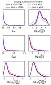 |
Fig. 12. Same as Fig. 11 but for the Varying Ar scenario. |
| In the text | |
|
Fig. A.1. Marginalised probability distribution of the IGM parameters of the disfavoured models for a constant exclusion likelihood. The red and blue curves refer to the Single-z and Joint-z cases at z = 9.1, respectively. The solid curves represent results from the main text, while the dashed refers to cases where we have used ℒex, single − z(θ, z = 9.1) = 0.5 and ℒex, joint − z(θ, z = 9.1) = 0.5. |
| In the text | |
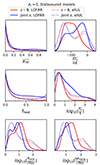 |
Fig. B.1. Same as Fig. B.2 but for z ∼ 8. |
| In the text | |
|
Fig. B.2. Marginalised probability distribution of the disfavoured models’ IGM parameters at z ∼ 10 for the allUL and Ar = 0 scenario. The red and blue curves refer to the Single-z and Joint-z cases, respectively. The solid curves represent results when we consider LOFAR upper limits only, while the dotted curves refer to cases where we have used all available upper limit results from different radio interferometric observations. |
| In the text | |
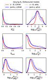 |
Fig. B.3. Same as Fig. B.1 but for the Varying Ar scenario. |
| In the text | |
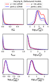 |
Fig. B.4. Same as Fig. B.2 but for Varying Ar scenario. |
| In the text | |
|
Fig. C.1. A subset of 1000 power spectra simulated with GRIZZLY at z = 9.1. These power spectra correspond to those with Ar = 0. The red and magenta points refer to the recent LOFAR 1σ upper limits from Mertens et al. (2025) and Acharya et al. (2024c), respectively. As a reference, the red dashed line corresponds to the power spectrum for a completely neutral IGM with no X-ray heating and TS = TK. |
| In the text | |
|
Fig. C.2. Posterior distribution of the source parameters at z = 9.1 for the Varying Ar scenario. These models are favoured by the LOFAR upper limits from Acharya et al. (2024c). Magenta indicates the case in which upper limits in three k−bins are considered, while teal represents the case when only one k−bin is used. The contour levels in the two-dimensional contour plots refer to the 1σ and 2σ credible intervals of the models favoured by the LOFAR upper limit at this redshift. The diagonal panels represent the corresponding marginalised probability distributions of each parameter. |
| In the text | |
|
Fig. C.3. Posterior distribution of the IGM parameters at z = 9.1 for the Varying Ar scenario. These posterior distributions correspond to the models that are favoured by the LOFAR upper limits from Acharya et al. (2024c). Magenta indicates the case in which upper limits in three k−bins are considered, while teal represents the case when only one k−bin is used. The contour levels in the two-dimensional contour plots refer to the 1σ and 2σ credible intervals of the models favoured by the LOFAR upper limits at this redshift. The diagonal panels represent the corresponding marginalised probability distributions of each parameter. |
| In the text | |
Current usage metrics show cumulative count of Article Views (full-text article views including HTML views, PDF and ePub downloads, according to the available data) and Abstracts Views on Vision4Press platform.
Data correspond to usage on the plateform after 2015. The current usage metrics is available 48-96 hours after online publication and is updated daily on week days.
Initial download of the metrics may take a while.