| Issue |
A&A
Volume 698, June 2025
|
|
|---|---|---|
| Article Number | A186 | |
| Number of page(s) | 32 | |
| Section | Extragalactic astronomy | |
| DOI | https://doi.org/10.1051/0004-6361/202554158 | |
| Published online | 13 June 2025 | |
Deeper multi-redshift upper limits on the epoch of reionisation 21 cm signal power spectrum from LOFAR between z = 8.3 and z = 10.1
1
LUX, Observatoire de Paris, PSL Research University, CNRS, Sorbonne Université, F-75014 Paris, France
2
Astron, PO Box 2, 7990 AA Dwingeloo, The Netherlands
3
Kapteyn Astronomical Institute, University of Groningen, PO Box 800, 9700 AV Groningen, The Netherlands
4
Department of Natural Sciences, The Open University of Israel, 1 University Road, PO Box 808, Ra’anana 4353701, Israel
5
Max-Planck Institute for Astrophysics, Karl-Schwarzschild-StraSSe 1, 85748 Garching, Germany
6
INAF – Istituto di Radioastronomia, Via P. Gobetti 101, 40129 Bologna, Italy
7
School of Physics and Astronomy, The University of Nottingham, University Park, Nottingham, NG7 2RD, UK
8
Department of Physical Sciences, Indian Institute of Science Education and Research Kolkata, Mohanpur, WB 741 246, India
9
Van Swinderen Institute for Particle Physics and Gravity, University of Groningen, Nijenborgh 4, 9747 AG Groningen, The Netherlands
10
Nordita, KTH Royal Institute of Technology and Stockholm University, Hannes Alfvéns väg 12, SE-106 91 Stockholm, Sweden
11
Laboratoire de Physique de l’Ecole Normale Supérieure, ENS, Université PSL, CNRS, Sorbonne Université, Université de Paris, F-75005 Paris, France
12
Astronomy Centre, Department of Physics and Astronomy, Pevensey II Building, University of Sussex, Brighton BN1 9QH, UK
13
Ru¯der Bošković Institute, Bijenička cesta 54, 10000 Zagreb, Croatia
14
School of Physics and Electronic Science, Guizhou Normal University, Guiyang 550001, PR China
15
Guizhou Provincial Key Laboratory of Radio Astronomy and Data Processing, Guizhou Normal University, Guiyang 550001, PR China
16
The Oskar Klein Centre, Department of Astronomy, Stockholm University, AlbaNova, SE-10691 Stockholm, Sweden
⋆ Corresponding authors: This email address is being protected from spambots. You need JavaScript enabled to view it.
; This email address is being protected from spambots. You need JavaScript enabled to view it.
Received:
17
February
2025
Accepted:
20
April
2025
Abstract
We present new upper limits on the 21 cm signal power spectrum from the epoch of reionisation (EoR), at redshifts z≈10.1,9.1, and 8.3, based on reprocessed observations from the Low-Frequency Array (LOFAR). The analysis incorporates significant enhancements in calibration methods, sky model subtraction, radio-frequency interference (RFI) mitigation, and an improved signal separation technique using machine learning to develop a physically motivated covariance model for the 21 cm signal. These advancements have markedly reduced previously observed excess power due to residual systematics, bringing the measurements closer to the theoretical thermal noise limit across the entire k-space. Using comparable observational data, we achieve a two- to fourfold improvement over our previous LOFAR limits, with best upper limits of Δ212 < (68.7 mK)2 at k=0.076 h cMpc−1, Δ212 < (54.3 mK)2 at k=0.076 h cMpc−1, and Δ212 < (65.5 mK)2 at k=0.083 h cMpc−1 at redshifts z≈10.1,9.1, and 8.3, respectively. These new multi-redshift upper limits provide new constraints that can be used to refine our understanding of the astrophysical processes during the EoR. Comprehensive validation tests, including signal injection, were performed to ensure the robustness of our methods. The remaining excess power is attributed to residual foreground emissions from distant sources, beam model inaccuracies, and low-level RFI. We discuss ongoing and future improvements to the data processing pipeline aimed at further reducing these residuals, thereby enhancing the sensitivity of LOFAR observations in the quest to detect the 21 cm signal from the EoR.
Key words: methods: data analysis / techniques: interferometric / cosmology: observations / dark ages, reionization, first stars
© The Authors 2025
 Open Access article, published by EDP Sciences, under the terms of the Creative Commons Attribution License (https://creativecommons.org/licenses/by/4.0), which permits unrestricted use, distribution, and reproduction in any medium, provided the original work is properly cited.
This article is published in open access under the Subscribe to Open model. This email address is being protected from spambots. You need JavaScript enabled to view it. to support open access publication.
1. Introduction
The period following the recombination era (z∼1100) represents one of the last unexplored frontiers in modern astronomy and cosmology. The epochs starting after the cosmic Dark Ages (z>30) encompass the formation of the first stars and galaxies during the cosmic dawn (CD; 15<z<30), and the epoch of reionisation (EoR; 6<z<15), marking the last major phase transition of the Universe (Barkana & Loeb 2001; Furlanetto et al. 2006; Loeb & Furlanetto 2013). Understanding these epochs is crucial for a comprehensive picture of cosmic evolution.
Our knowledge of these early times remains limited, primarily due to the scarcity of detectable luminous sources at such high redshifts. Recent observations, particularly from the James Webb Space Telescope (JWST), have begun to unveil galaxies at redshifts of z>10, pushing the boundaries of our observational capabilities (e.g. Bouwens et al. 2023; Harikane et al. 2023; Atek et al. 2023; Donnan et al. 2023; Finkelstein et al. 2024). These observations have revealed a surprisingly abundant population of bright galaxies in the early Universe, challenging existing models of galaxy formation and evolution (Boylan-Kolchin 2023; Mason et al. 2023; Arrabal Haro et al. 2023).
Central to exploring these eras is the observation of the redshifted 21 cm line of neutral hydrogen, which promises to chronicle the first billion years of the Universe's evolution. Such observations can yield invaluable insights into cosmic history, the formation of the first luminous structures, and the properties of the sources driving reionisation. By tracing the HI gas in the intergalactic medium (IGM), we can study the cumulative impact of these light sources, not just the brightest ones (for reviews see e.g. Ciardi & Ferrara 2005; Morales & Wyithe 2010; Pritchard & Loeb 2012; Furlanetto et al. 2016). These observations may even unveil entirely new physics, such as exotic heating mechanisms or interactions in the dark sector (e.g. Barkana 2018; Fialkov & Barkana 2019).
Current evidence suggests that most of the reionisation occurred within 6≲z≲10, as is indicated by the Gunn-Peterson trough in high-redshift quasar spectra (e.g. Becker et al. 2001; Fan et al. 2006; Eilers et al. 2018) and measurements of the Thomson scattering optical depth of the cosmic microwave background (CMB) radiation (Planck Collaboration VI 2020). Recent analyses, particularly those examining IGM damping wing absorption in quasar spectra, imply a rapid evolution of the EoR between 5.5<z<7 (e.g. Greig et al. 2017; Davies et al. 2018; Bañados et al. 2018; Wang et al. 2020). Observations of the Lyα forest at z∼6 suggest that the EoR extended down to z∼5.5 (Becker et al. 2015; Bosman et al. 2018; Keating et al. 2020; Qin et al. 2021). These findings align with CMB constraints, supporting a relatively late EoR with a midpoint around z∼7 (e.g. Greig et al. 2017; Qin et al. 2020). Nonetheless, much remains to be understood about the EoR, and the observation of the 21 cm signal from this epoch could provide critical insights into these formative periods of the Universe.
Large low-frequency radio telescopes such as LOFAR1 (van Haarlem et al. 2013), MWA2 (Tingay et al. 2013), NenuFAR3 (Zarka et al. 2020), HERA4 (Deboer et al. 2017), and GMRT5 (Gupta et al. 2017) are at the forefront of the search for the 21 cm signal across a broad range of redshifts. Initially, these experiments have aimed for a statistical detection of the 21 cm fluctuations. These efforts are also crucial for the success of the forthcoming SKAO6, a next-generation radio telescope with unmatched sensitivity and with the potential to obtain images of these epochs (Koopmans et al. 2015; Mellema et al. 2015). Despite significant challenges, these instruments have set impressive upper limits on the 21 cm signal power spectra, but they have yet to achieve a detection. Recent efforts include those by Trott et al. (2020), who reported a 2-σ upper limit of 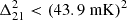 at z≈6.5 and k=0.15 h cMpc−1 with the MWA, using 298 h of carefully selected data, and the HERA team, who recently reported a 2-σ upper limit of
  at z≈7.9 and k=0.34 h cMpc−1, and
 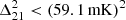 at z≈10.4 and k=0.36 h cMpc−1using 94 nights of observations (HERA Collaboration 2023). The LOFAR-EoR Key Science Project has also made significant progress. We published a first upper limit based on 13 hours of data (Patil et al. 2017). This was later improved to a 2-σ upper limit at z≈9.1 of
 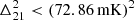 at k=0.075 h cMpc−1, using 141 hours of data (Mertens et al. 2020, hereafter LOFAR20).
Detecting the 21 cm signal is extremely challenging due to the difficulty of extracting this faint signal buried beneath astrophysical foregrounds that are many orders of magnitude brighter and contaminated by numerous systematics. At the low radio-frequencies targeted by 21 cm signal observations, the emission from the Milky Way and other extra-galactic sources dominates the sky. The emission of these foregrounds varies smoothly with frequency, which can be used to differentiate it from the rapidly fluctuating 21 cm signal (Jelić et al. 2008). However, the frequency-dependent response of the radio telescopes introduces structure to the otherwise spectrally smooth foregrounds, causing so-called ‘mode-mixing’ (Morales et al. 2012). Most chromatic effects are confined inside a wedge-like shape in k-space (Datta et al. 2010; Trott et al. 2012; Vedantham et al. 2012; Liu et al. 2014). High-precision calibration is essential, as errors can be introduced by calibration with an incomplete or incorrect sky model (Patil et al. 2016; Ewall-Wice et al. 2017; Barry et al. 2016), incorrect bandpass calibration, and cable reflections (Beardsley et al. 2016), as well as chromatic errors due to leakage from the polarised sky into Stokes-I (Jelić et al. 2010; Spinelli et al. 2018), ionospheric disturbances (Koopmans 2010; Vedantham & Koopmans 2016; Jordan et al. 2017; Mevius et al. 2016; Brackenhoff et al. 2024), incorrect primary-beam models (Gehlot et al. 2021; Chokshi et al. 2024), or gridding errors (Offringa et al. 2019b). Multi-path propagation, mutual coupling (Kern et al. 2020; Kolopanis et al. 2023), and residual radio-frequency interference (RFI) (Offringa et al. 2019a; Wilensky et al. 2019) must also be corrected or mitigated with great precision to detect the redshifted 21 cm signal.
Various observing and analysis strategies have been implemented by different teams, to optimise the telescope's capabilities and ensure the successful detection of the 21 cm line. The strategy of the LOFAR-EoR Key Science Project involves combining thousands of observing hours on a deep field, calibrated to high precision with a deep and extended sky model of the field using a sky-based calibration scheme. We also pursue a foreground removal strategy to model and remove foreground contaminants, aiming to probe the 21 cm signal both outside and inside the foreground wedge, enhancing sensitivity and accessing larger scales. This effort requires a comprehensive sky model. In this work, we focus on one of the deep fields studied by the LOFAR-EoR Key Science Project; namely, the north celestial pole (NCP). The model (Yatawatta et al. 2013; Patil et al. 2017) of this field currently consists of almost thirty thousand components. This model is used for solving station gains in multiple directions using the Sagecal-CO code (Yatawatta 2016) and subsequently removing these components with their direction-dependent (DD) instrumental response functions. Residual foregrounds are then statistically separated from the 21 cm signal using Gaussian process (GP) regression (GPR, Mertens et al. 2018, 2024).
This strategy was implemented by LOFAR20, where, despite setting scientifically interesting upper limits and discarding some extreme models (Ghara et al. 2020; Greig et al. 2021; Mondal et al. 2020), the results were still above the theoretical limits expected if thermal noise dominated. Over the past four years, many potential sources of this excess have been investigated, including residual foreground emissions from off-centre sources, chromatic direction-independent (DI) and DD calibration errors, low-level RFI, and ionospheric disturbances. Detailed analyses by Gan et al. (2022) showed that the excess variance was not strongly correlated with gain variance or ionospheric conditions, suggesting that neither calibration errors nor ionospheric effects are the primary contributors. This finding was corroborated by Gan et al. (2023), who found no significant difference in foreground removal between two calibration algorithms, and by Brackenhoff et al. (2024), who demonstrated that ionospheric impact on cylindrically averaged power spectra is confined to the wedge and can be effectively modelled and removed using current techniques. However, Gan et al. (2022) indicated that the excess variance might be related to bright, distant sources such as Cassiopeia A (Cas A) and Cygnus A. Additionally, Hothi et al. (2021) found that the GPR method was optimal compared to alternatives, although Kern & Liu (2021) highlighted the need for a more physically motivated approach to GPR to reduce the risk of bias and signal loss.
Although we have not yet definitively identified the cause of the observed excess power in our data, these recent analyses have provided valuable insights into potential contributing factors, leading to significant enhancements in our processing pipeline. These include improvements in both DI and DD-calibration, more effective RFI flagging, and enhanced residual foreground removal methods. In particular, the latter benefited from several recent works: Mertens et al. (2024) introduced the concept of learned kernels, which allows for a parametrised covariance function to be derived from simulated datasets, ensuring a more physically motivated model and significantly improving component separation. This new ML-GPR method was first tested on LOFAR simulations (Acharya et al. 2024a) and then applied to LOFAR data in Acharya et al. (2024b).
In this publication, we present improved multi-redshift 21 cm power spectrum upper limits from the LOFAR-EoR Key Science Project. These new upper limits are based on a similar set of observations as were used in our LOFAR20 publication (about 140 h of data) but include a broader frequency range (122–159 MHz). This broader range allows us to set upper limits at redshifts centred on z≈10.1,9.1, and 8.3.
Our observational strategy is detailed in Section 2, with the processing and analysis methods described in Section 3. A new upper limit on the 21 cm signal power spectra is presented in Section 4, and the validation procedure is explained in Section 5. Finally, we discuss our results and their implications in Section 6. Throughout this paper, we use a ΛCDM cosmology consistent with the Planck 2015 results (Planck Collaboration XIII 2016).
2. Observations
The LOFAR radio telescope comprises 24 core stations distributed within a 2 km diameter, 14 remote stations across the Netherlands, providing a maximum baseline length of approximately 100 km, and an increasing number of international stations across Europe (van Haarlem et al. 2013). The LOFAR-EoR observations utilise the High Band Antennas (HBA), operating at frequencies between 110 and 189 MHz, and target two primary fields: the NCP and the bright compact radio source 3C 196 (de Bruyn 2012).
We reanalysed 12 NCP observations from LOFAR Cycles 0 to 3, which were previously used in LOFAR20, along with two additional nights from Cycles 1 and 2. This amounts to about 200 hours of observation. The NCP is particularly advantageous for EoR studies due to its year-round continuous visibility, making it a key focus for deep field observations. These observations employed all core stations (in split mode, effectively providing 48 stations) along with remote stations. The observational setup remained nearly identical to that described in LOFAR20. Data were recorded with a frequency range of 115–189 MHz, a spectral resolution of 3.05 kHz (resulting in 64 channels per sub-band of 195.3 kHz), and a temporal resolution of 2 seconds. Key differences from the LOFAR20 analysis include the processing of two additional frequency bands – 122–134 MHz and 147–159 MHz – alongside the previously used 134–147 MHz band, as well as the inclusion of two additional nights of observations. All frequency bands were reprocessed using an updated processing pipeline, which is detailed in the subsequent sections. A summary of all observations is provided in Table 1.
List of all observation nights analysed, with date, time, duration, and noise statistics.
3. Data reduction
The LOFAR-EoR data processing pipeline has been iteratively developed and generally follows the strategy described by Patil et al. (2017) and LOFAR20. It comprises the following key steps: (i) Pre-processing, where visibility averaging and RFI excision are performed; (ii) Calibration, involving a DI calibration scheme using a sky-based approach; (iii) Sky-model source subtraction, employing DD calibration for accurate source removal; (iv) Post-calibration flagging, which includes further RFI excision; (v) Imaging, converting visibilities into image cubes in units of Kelvin; (vi) Combination of nights, where data from multiple nights are combined using an inverse variance-weighted method; and finally, (vii) Residual foreground removal, which models the gridded observed data as a sum of multiple components: foregrounds, excess emissions, and the 21 cm signal. The foreground component was removed, and the residual formed the basis for our upper limit on the 21 cm power spectrum.
This study introduces several improvements, particularly in the calibration steps, sky model subtraction, and post-calibration flagging strategy. A new method for residual foreground subtraction was also implemented. Figure 1 shows an overview of the LOFAR-EoR data processing pipeline. All data processing was conducted on the ‘Dawn’ compute cluster, equipped with 48 × 32 hyperthreaded compute cores and 124 Nvidia K40 GPUs, located at the Centre for Information Technology of the University of Groningen.
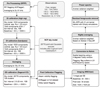 |
Fig. 1. LOFAR-EoR HBA processing pipeline, describing the steps required to reduce the raw observed visibilities to the 21 cm signal power spectra. |
3.1. Pre-processing
The raw LOFAR NCP data were initially integrated with a time resolution of 2 seconds and 64 channels per sub-band. After applying RFI flagging using AOFlagger (Offringa et al. 2012) and excluding the outer 2 channels on both sides of the band, the data were averaged to 15 channels of 12.2 kHz per sub-band before archiving in the LOFAR Long Term Archive (LTA). As is described in LOFAR20, a second AOFlagger step was performed before further averaging to three channels of 61 kHz width. Intra-station baselines, affected by crosstalk due to shared electronics cabinets, were also fully flagged. To stabilise the initial calibration, the raw data were pre-scaled such that the visibility amplitudes were between 1 and 10. This step made sure that the initial gains, initialised with an amplitude of 1 and phase of zero, were within a factor of 10 of the final optimised gains. The resulting data product, averaged over three channels with a resolution of 2 seconds, was then used in the initial calibration step.
3.2. Calibration
For calibration, we used a sky model similar to that described in LOFAR20, with the exception of modified models for the three brightest sources (3C 61.1, Cas A, and Cygnus A) and a reduced number of components and clusters. Details of these modifications are provided below. The intensity scale of the sky-model is set by NVSS J011732+892848 (RA 01h 17m 33s, Dec 89° 28′ 49″ in J2000), as was the case in LOFAR20.
The spectral variability of the bright 3C 61.1 source near the first null of the beam would dominate the calibration solutions in the rest of the field. Therefore, similar to LOFAR20, the DI calibration step treats the 3C 61.1 direction separately. It solves simultaneously for the station gains in two directions and then corrects the visibilities with the gain solutions of the central field. We solved for a 2 × 2 complex gain (i.e. Jones) matrix per station, using a ∼1300 component model of the central field as well as an updated model consisting of 1545 clean components for 3C 61.1 (Ceccotti et al. 2023). The model consists of intrinsic flux density values, and the station beam response was modelled from the geometrical delays using the positions of the individual dipoles (i.e. the array factor). Tiles that were flagged during the observations were taken into account in the beam response model, but individual malfunctioning dipoles are not. In this way, the dipole response including any cross coupling effects were absorbed in the gain solutions and thus applied when using the gains to correct the visibilities.
Sagecal-CO (Yatawatta 2016) was used to calibrate our observations, which allowed us to regularise the spectral behaviour of the gain solutions in order to approach a smooth curve with a regularisation prior. We used a third-order Bernstein polynomial over the 13-MHz bandwidth, treating each redshift bin separately. Variation in the Sagecal-CO regularisation parameter determines how fast the solutions converge to this smooth curve. In LOFAR20 almost full spectral freedom was allowed during DI-calibration by setting a low regularisation parameter and only relatively few iterations. It is known that spectral errors in the gains that are applied when correcting the visibilities can introduce unwanted features in the final power spectrum that cannot be removed in later steps in the processing. Unmodelled sky components can for example be the cause of such errors in the gains (e.g. Barry et al. 2016). Following Mevius et al. (2022), a high spectral regularisation of the gains is desired. However, small spectral features, such as cable reflections, with a typical frequency scale of ∼1 MHz for LOFAR HBA data, require solutions with high spectral resolution. Those features, however, are expected to be fairly constant in time and direction. We therefore adopted a two-step approach:
-
(i)
DI-calibration with high spectral regularisation – First, DI spectrally smooth solutions were fitted using Sagecal-CO with a high-regularisation parameter and a solution time interval of 30 s.
-
(ii)
Bandpass calibration – Subsequently, a full bandpass calibration was performed with a single solution per sub-band and a time interval of 4 hours. This interval was chosen due to computational limitations, although ideally the entire observation duration would be used.
We note that a simultaneous solve for long and short term solution intervals would also be computationally impossible. Therefore, this iterative approach was chosen. The preferred order of the two-step approach, first high-regularisation then bandpass calibration, was based on experiments on actual data. Convergence of the solutions was most stable this way and experiments showed no further improvement after a second iteration of high-regularisation calibration.
The sky model is more accurate on the shorter baselines, where it is less affected by ionospheric errors (e.g. Vedantham & Koopmans 2016; Mevius et al. 2016; Ewall-Wice et al. 2017; Brackenhoff et al. 2024). Therefore, we decided to limit the baseline range of the visibilities used in the DI-calibration to 50–5000λ. This choice includes all LOFAR core baselines and is based on experiments testing the final power spectrum of a single night of observation with various baseline cuts and solution time intervals. Importantly, this baseline length is comparable to or smaller than the typical ionospheric diffractive scale at our observing frequency (Mevius et al. 2016), minimising the impact of ionospheric phase fluctuations. A more rigorous analysis of the optimal baseline selection using a full simulation of the processing pipeline will be the topic of a follow up paper.
Figure 2 shows the gain spectra of the DI-calibration solution for a typical observation night. It demonstrates a significant reduction in gain errors by two to three orders of magnitude compared to LOFAR20, while preserving the correction of spectrally non-smooth but time-stable features in the signal processing chain (e.g. cable reflections), which are properly accounted for.
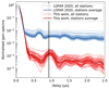 |
Fig. 2. Normalised gain-spectra of the DI-calibration for frequency range 134–147 MHz, observation L254871. The one-step unregularised calibration (‘LOFAR 2020’, blue lines) is compared with the two-steps calibration (‘This work’, red lines). The delay corresponding to reflections in the 115-metre cables of LOFAR is denoted by a grey line, where a spectral feature is also observed, as expected. |
3.3. Sky-model sources subtraction
In the second calibration step, no corrections were applied to the data. Instead, an extensive model, consisting of 28 778 components, was subtracted from the visibilities after multiplication with the fitted DD-gains. As was the case in LOFAR20, we fitted the DD-gains on a different set of baselines than the ones used in the final power spectrum. We calibrated our data on the baselines between 250 and 5000 λ, while the final power spectrum used the baselines below 250 λ. The reason for this is twofold: first, this method ensures that the 21 cm signal of interest is not suppressed while subtracting the gain-corrected model (Sardarabadi & Koopmans 2019; Mevius et al. 2022), and secondly, our sky model does not include the large diffuse structures which mainly affect the shorter baselines that are excluded from the gain calibration. The DD-calibration closely follows that of LOFAR20 with a few alterations highlighted here.
LOFAR20 used a 28 773 component model divided into 122 separate clusters, where the 2×2 complex station gains in the direction of each individual cluster were solved for simultaneously using Sagecal-CO. In this work, we modified that model in several ways. Firstly, we found that residuals from the bright A-team sources (Cas A and Cygnus A) significantly contributed to excess variance in the power spectrum (Gan et al. 2022). We therefore updated their model, replacing shapelet components with a simpler mix of point sources and Gaussians, which improved results, although the exact reason for this improvement is still under investigation (Ceccotti et al. 2025a). Secondly, clusters outside the first station beam null showed higher variance in the solutions, likely due to rapid beam-related gain fluctuations that cannot be accurately captured by the spectrally smooth gains used in Sagecal-CO. In such cases, including these clusters can increase, rather than reduce, the overall variance. By excluding 14 outer clusters from the DD-calibration (see Figure 3), we achieved a marked improvement in the final power spectrum. The updated model now contains 28 778 components in 108 clusters.
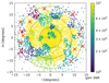 |
Fig. 3. Signal-to-noise ratio (S/N) of the time-differenced solutions for all ∼28 000 sky components of LOFAR20 in real data. Clusters of components can be recognised since they share the same gain solutions. In total, there are 120 clusters in the image. The S/N is similar for most clusters, but showing a slight gradient to lower S/N values away from the phase centre. The components in the outer 14 clusters (with a flux weighted mean position more than 10 degrees away from the phase centre), indicated with red crosses, have been removed from the model used in the current analysis. |
Similar to LOFAR20, we used Sagecal-CO with high-regularisation parameters optimised to minimise the gain variations per individual cluster. The solution time interval varies between 2.5 and 20 min depending on the total apparent flux in a cluster. To ensure maximum smoothness, fitted smooth third-order Bernstein polynomials were used instead of the regularised gains, which may still contain higher-frequency spectral features7. The sky-model multiplied with these smooth gains was then subtracted from the visibilities for further processing.
3.4. Post-calibration flagging
In the LOFAR20 analysis, we also encountered a substantial amount of low-level RFI, which we believe significantly contributed to the excess power observed on small baselines. Some measures were implemented in the previous analysis to mitigate this impact. Notably, we systematically flagged certain small baselines that were visibly heavily affected by RFI. Subsequent near-field imaging (see Smeenk 2020, for the methodology) confirmed that the source of this interference was local to the superterp8. In the current analysis, we aimed to improve upon this approach by automating the detection and flagging of low-level RFI. Our post-processing flagging procedure included the following steps:
Wide bandwidth AOFlagger: The AOFlagger algorithm (Offringa et al. 2012) was applied, post point-source subtraction, across the full frequency band of each of the three redshift bins. This increases our sensitivity to fainter and broadband RFI. The effect of this step is shown in the second panel of Figure 5, where RFI contamination along the horizon line and within the foreground wedge is visibly reduced.
Timeslots flagging: Timeslots with more than 35% of flagged data and baselines with over 80% of flagged data are fully flagged, with the aim of minimising the impact of flagging caused by missing frequency channels. The issue with missing frequency channels arises because flagged samples introduce spectral discontinuities, causing excess power when the data are averaged or gridded, which can bias the 21 cm power spectrum (Offringa et al. 2019a).
Flag RFI in the 147–149 and 155–158 MHz bands: By visual inspection, we noticed that some baselines were affected by broadband RFI in these bands. The detection and flagging of this RFI was automated using a statistical thresholding based on the mean power ratio inside and outside the band. The number of flagged baselines for this step is shown in the shaded and blank bars in Figure 4. Typically, only a few baselines were affected by this RFI. The 147–149 MHz band RFI mostly affects earlier observations (cycles 0 to 2), while the 155–158 MHz band RFI primarily affects cycles 2 and 3, impacting not only small baselines but also longer ones. An example of the baselines affected by this type of RFI is presented in Appendix A.
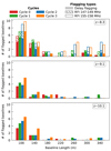 |
Fig. 4. Number of flagged baselines by some of the post-calibration visibility flagger, grouped by baseline length bins and categorised by different sources of contamination. Short baselines are predominantly affected, although certain frequency bands (147–149 MHz and 155–159 MHz) also show contamination on longer baselines |
Delay-space baseline flagger: Finally, a systematic search for RFI-corrupted baselines was conducted. This involved computing the delay spectra for each baseline individually, analysing the median amplitude over time above the horizon limit, and flagging baselines that showed outlier peaks beyond a set threshold. The effect of this step is shown in the third panel of Figure 5. The number of flagged baselines for this step is represented by the plain bars in Figure 4. Examples of baselines flagged by this method are presented in Appendix A. Although it results in a non-negligible increase in thermal noise on these baselines due to fully flagging entire baselines, the benefit of reducing these contaminants far outweighs the cost. For future work, we are investigating the possibility of filtering these contaminants – mainly from local RFI sources – to preserve as much data as possible.
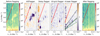 |
Fig. 5. Effect of post-calibration flagging steps on the 2D power spectra for observation L246309 in the frequency range 134–147 MHz. The left panel shows the power spectra before any calibration. The four middle panels display the ratio of power spectra before and after each successive flagging step, illustrating the progressive reduction of contamination. The four steps, shown in order, are: (1) post-calibration wide-bandwidth AOFlagger; (2) baseline flagging of delay-spectrum outliers above the horizon limit; (3) post-gridding flagging based on outlier detection in channels and uv-cells; and (4) post-gridding flagging of uv-cells contaminated by A-team sidelobes. The right panel shows the power spectra after all steps have been applied. While some steps increase thermal noise (e.g. step 2, which removes entire baselines), they are effective in reducing RFI-related contamination. In all panels, the foreground horizon line is shown as a solid red line, while the dashed green and black lines indicate the delay ranges where most of the power from Cas A and Cygnus A is expected, respectively. |
The cumulative effect of these flagging steps, in addition to other flagging steps on the gridded visibility cubes described later, is shown in Figure 5.
3.5. Imaging
After calibration, source subtraction, and RFI excision, the residual visibilities were gridded and imaged independently for each sub-band using WSClean9 (Offringa et al. 2014), producing an (l,m,f) image cube, with f the frequency. Separate Stokes-I and V images (in Jy PSF−1), as well as point spread function maps, were generated for each sub-band using natural weighting. Additionally, even and odd 10-second time-step images were created, enabling the generation of gridded time-differenced visibilities to estimate the thermal noise variance in the data. The sub-bands were then combined into image cubes with an 8.5°×8.5° field of view and a pixel size of 0.5 arcmin. These cubes were trimmed using a Tukey spatial filter with a 4° diameter, focusing on the primary beam's most sensitive region (the station's primary beam full width at half-maximum at 140 MHz is approximately 4.1°). The Tukey window was chosen to find a compromise between avoiding sharp image edges and maximising the observed volume, thereby improving sensitivity.
The image cubes produced by WSClean were converted to Kelvin units following the procedure outlined in LOFAR20, and then transformed back to gridded visibilities through an inverse Fourier transform applied independently for each frequency channel. For each dataset, the gridded visibilities, V(u,v,f), were stored in a HDF5 format in Kelvin units, along with the number of visibilities that contribute to each (u,v,f) grid point, Nvis(u,v,f).
A final outlier rejection was performed on the gridded visibility cubes to flag any remaining low-level RFI using a simple threshold-clipping method. Channels were flagged based on outliers in Stokes-V and Stokes-I variance. The flagged frequencies for the three redshift bins are shown in Figure 6 (grey areas). Many channels were flagged in the z≈9.1 redshift bin, while the z≈10.1 bin is comparatively cleaner. uv-cells are also flagged based on outliers in the weights, Stokes-V variance, and channel-difference Stokes-I variance. Additionally, uv-cells corresponding to sidelobes originating from Cas A and Cygnus A in uv-space were flagged (see Munshi et al. 2025b, for a formal mathematical treatment of this effect). The flagged uv-cells for the three redshift bins are shown in Figure 7, and most flagging is due to Cas A and Cygnus A. The impact of this flagging on the cylindrically averaged power spectra is shown in Figure 5, which indicates that the A-team flagger primarily reduces power in regions where these sources are expected to contribute, helping to reduce contaminants.
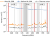 |
Fig. 6. Variance as function of frequency for the ten combined nights of the three redshift bins. The top line (blue) shows the Stokes-I power after sky-model subtraction (DD-calibration). The middle line (orange) shows the variance of the residual after ML-GPR, the bottom line (dark grey) show the thermal noise level estimated from the gridded time-differenced visibilities. Flagged channels are shown in light grey. |
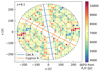 |
Fig. 7. Noise standard deviation, in SEFD units, estimated from the channel-differenced noise at each uv-cell, after sky-model subtraction. Data are shown for the Stokes-I 10 nights combined z≈9.1 data cube. The trace of the Cas A and Cygnus A sources in the uv plane, which are fully flagged, are denoted with a blue and orange line, respectively. |
3.6. Combining nights
To achieve a better sensitivity and reduce thermal noise (and other incoherent errors), combining data from multiple nights of observation is essential. In this analysis, data from 14 nights were processed, but only the best 10 nights for each redshift bin were selected for combination. This allow us to be consistent with the LOFAR20, while also allowing for the exclusion of clearly suboptimal nights. The selected nights are listed in Table 1. This selection was based on the quality of each nights, as is reflected in the post-calibration cylindrically averaged power spectra (see Appendix B for a complete list of cylindrically averaged power spectra for all analysed nights).
The selected nights were combined at the visibility level, following the weighting scheme:
where Vi represents the visibility cube for the i-th night, Vcn is the combined visibility cube for n nights, and Wi is the weights cube for the i-th night indicating the effective number of visibilities contributing to each uv-grid point.
3.7. Residual foreground removal
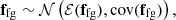
After calibration and sky-model source subtraction, the residual Stokes-I visibilities, Vres, are still dominated by foregrounds, predominantly extra-galactic emission below the confusion limit and partially polarised diffuse Galactic emission. These foregrounds are approximately three orders of magnitude brighter than the 21 cm signal. Following the methodology of LOFAR20, we applied GPR (Rasmussen & Williams 2006) to model and subtract the residual foregrounds. This approach exploits the distinct frequency coherence scales of the foregrounds and the 21 cm signal, and follow the methodology established in Mertens et al. (2018). The data, d, were modelled as:
 (1)
(1)
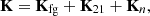
where the vectors ffg, f21, and n represent the foregrounds, 21 cm signal, and noise components, respectively, as functions of the frequency, f. The different components, which we assume to be independent, can be separated based on their distinct spectral behaviour (Mertens et al. 2018)10. This behaviour is defined by the covariance of the components between frequency channels. The total frequency-frequency covariance matrix of the data, K, is a sum of the individual covariance matrices, encompassing the foreground covariance matrix, Kfg, the 21 cm covariance matrix, K21, and the noise covariance matrix, Kn:
 (2)
(2)
using the shorthand K≡K(f,f). The joint probability density distribution of the observations, d, and the function values, ffg, of the foreground model at the same frequencies, f, are then given by
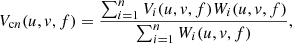
![Mathematical equation: $$ \left [\begin {array}{c} {{\mathbf {d}}} \\ {{\mathbf {f}}}_{{\mathrm {fg}}} \end {array}\right ] \sim {\cal {{N}}}\left (\left [\begin {array}{c} {{\mathbf {0}}} \\ {{\mathbf {0}}} \end {array}\right ], \left [\begin {array}{cc} {{\mathbf {K}}}_{{\mathrm {fg}}} + {{\mathbf {K}}}_{21} + {{\mathbf {K}}}_{{\mathrm {n}}} & {{\mathbf {K}}}_{{\mathrm {fg}}} \\ {{\mathbf {K}}}_{{\mathrm {fg}}} & {{\mathbf {K}}}_{{\mathrm {fg}}} \end {array}\right ] \right ). $$](/articles/aa/full_html/2025/06/aa54158-25/aa54158-25-eq11.gif) (3)
(3)
The foreground model is then a GP, conditional on the data:
 (4)
(4)
with an expectation value and covariance defined by:
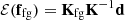 (5)
(5)
 (6)
(6)
The residual was obtained by subtracting ℰ(ffg) from the observed data:
 (7)
(7)
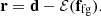
The GPR method utilises parametrised covariance functions to model the different components of the signal. These functions are defined by a set of parameters, θ, which control properties such as variance and the overall shape of the covariance function. In GPR, we performed prior covariance model selection under a Bayesian framework by choosing the model that maximises the log-marginal-likelihood.
 (8)
(8)
with n the number of data points. The posterior probability density of the parameters was then estimated by applying Bayes’ theorem, incorporating the prior on the parameters:
 (9)
(9)
The posterior distributions for the parameters of our GP model were derived for each redshift bin with a nested sampling algorithm using the UltraNest11 package (Buchner 2021).
To enhance the robustness of our methodology, we have introduced several improvements over the LOFAR20 approach. One key limitation of the earlier approach was the reliance on an exponential covariance function to model the 21 cm signal. While this choice was effective for a subset of simulations, it risks introducing biases when applied to a wider range of scenarios (Kern & Liu 2021). In this work, we addressed this limitation by employing a machine learning approach to construct a physically motivated covariance function directly from simulations of the 21 cm with different astrophysics. Specifically, we used a variational autoencoder (VAE) to learn a low-dimensional representation of the 21 cm signal covariance from a large ensemble of simulations (Mertens et al. 2024). This enables a more accurate and flexible modelling of the 21 cm component in the data.
The simulations used for this training are based on the Grizzly framework (Ghara et al. 2015, 2018), which encompasses a wide range of astrophysical scenarios. The trained VAE kernel thus serves as an effective model for the 21 cm signal covariance matrix, parametrised by three key factors: two latent space dimensions, x1 and x2, and a variance scaling factor,  . This machine-learning-derived covariance function is integrated into our GPR framework to more accurately isolate the 21 cm signal from the foregrounds and systematics. We refer to Mertens et al. (2024) for a comprehensive description of the VAE method, and Acharya et al. (2024a) for the more specific description of the Grizzly trained VAE kernel.
For the foreground components, we used analytical covariance models from the Matérn class (Rasmussen & Williams 2006), which provide a flexible description of the spectral behaviour observed in the data. Different forms within the Matérn class, such as Matérn 3/2 and Matérn 5/2, have been tested through multiple trials to identify the most suitable model for our observations.
Additionally, to account for the baseline dependence of the foregrounds coherence scale (which manifests as the ‘wedge’ in k-space), we set the coherence scale as a function of baseline length using:
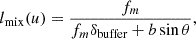 (10)
(10)
where lmix is the mode-mixing coherence-scale, δbuffer is the delay buffer, b is the baseline length, θ is the angular distance of foreground sources from the phase centre, and fm is the central frequency of the redshift bin.
The same range of covariance models has also been successfully used in the recent SKA Data Challenge 3a (Bonaldi et al. 2025), where they were tested on externally produced data and emerged as the top-performing approach. While this demonstrates the performance of the method, it should be noted that the challenge dataset was relatively simplified compared to real observational data.
Our findings indicate that the data cannot be adequately described by only the foreground and 21 cm components. There is additional power within the data characterised by a smaller coherence scale (typically of ≈0.4 MHz), making it more challenging to differentiate from the 21 cm signal. This necessitates the addition of an ‘Excess’ component to our covariance model to ensure a more effective separation between the foregrounds and the 21 cm signal.
The final parametric GP model is composed of five terms:
 (11)
(11)
where Kn represents the thermal noise diagonal covariance matrix, estimated from the time-differenced visibility cube, and α a scaling factor that accounts for additional frequency-uncorrelated noise in the data in excess of the thermal noise.
The various components and their parameters are detailed in Table 2. The model includes six main components:
-
(i)
The sky – Represents the large-scale spectrally smooth foregrounds, the astrophysical sources, Galactic and extra-galactic, in the field of view of the image cube.
-
(ii)
The Mode-mixing 1 – Accounts for chromatic effects with shorter coherence-scale introduced by the spectral response of the instrument.
-
(iii)
The Mode-mixing 2 – An additional mode-mixing component used exclusively for the z≈10.1 bin, as one component was insufficient to account for the chromatic effects for this redshift.
-
(iv)
The excess – Captures small-scale residual structures not fully accounted for by the foreground models.
-
(v)
The 21 cm – The learned component that should capture the 21 cm signal in the data.
-
(vi)
The noise – Represents the thermal noise inherent to the observation.
Each of these components has different associated parameters, for which we assigned prior ranges that were iteratively refined during model development. The prior ranges and the posterior values reflect our best understanding of the spectral behaviours of the foregrounds and excess components for each redshift bin, and ensure the separability between the 21 cm signal in one part and the foregrounds and instrumental effects in another part. In addition to selecting the model and prior ranges that would maximise the Bayesian evidence, this process is also guided by injection tests. It consists of injecting a mock 21 cm signal into the data and ensuring that it can be recovered by our component separation process (this procedure is fully described in Section 5).
GP model: summary of the model parameters, priors, and posteriors (median with 68% intervals).
3.8. Power spectra estimation
We define the cylindrically averaged power spectrum as (Mertens et al. 2020):
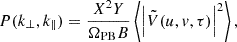 (12)
(12)
where  is the Fourier transform of the visibility cube V(u,v,f) in the frequency direction, B is the frequency bandwidth, ΩPB is the integral of the square of the primary beam gain over the solid angle, X and Y are conversion factors from angle and frequency to comoving distance, and <..> denotes the averaging over baselines inside a bin-width. The Fourier modes are in units of inverse comoving distance and are given by (Morales et al. 2006; Trott et al. 2012)
 (13)
(13)
where DM(z) is the transverse co-moving distance, H0 is the Hubble constant, f21 is the frequency of the hyperfine transition, and E(z) is the dimensionless Hubble parameter. We also define the dimensionless power spectrum by averaging the power spectrum in spherical shells as
 (14)
(14)
This representation is well suited for characterising the 21 cm signal, to a first order12. We limited our analysis to a bandwidth of 12 MHz to limit the effects of signal evolution; in other words, the light-cone effect (Datta et al. 2012).
When displaying the cylindrically averaged power spectra, we overplot the horizon line. This line represents the limit above which we do not expect any foreground emission and delimits the foreground wedge. The line was computed using improved calculations that take into account the sky curvature and phase-referencing away from zenith (Munshi et al. 2025b).
3.8.1. Uncertainty calculation
To compute the power spectrum and its uncertainty for a given ML-GPR component, such as the 21 cm signal for illustration as given below, we employed the following procedure:
-
1.
We drew m samples from the posterior distribution of the parameters obtained from the nested sampling results from the GPR analysis.
-
2.
For each set of parameters, we calculated the predictive mean, ℰ(f21), and the predictive covariance, cov(f21), of the 21 cm component.
-
3.
For each parameter sample, we generated a realisation of the 21 cm signal by adding a random fluctuation to the predictive mean:
 (15)
(15)where δ21 is a random vector drawn from a multivariate Gaussian distribution with covariance cov(f21).
-
4.
We computed the power spectrum for each realisation, f21, using the definitions provided earlier.
-
5.
After processing all m samples, we have m power spectra. We estimated the final power spectrum of the 21 cm component by calculating the median of these m spectra at each k value. The associated 1σ uncertainty was determined by the standard deviation of the power spectra values at each k.
This method accounts for uncertainties in the parameters and propagates them through to the power spectrum estimation. By incorporating the variability from both the parameters and the intrinsic fluctuations of the 21 cm signal, we obtained a more robust estimate of the power spectrum and its statistical uncertainty. We note that calibration gain errors were ignored in this calculation. Calibration errors manifest themselves as additional power (solver noise in the spectra when the solutions are transferred from longer to shorter baselines. Mevius et al. (2022) have shown that the expected level of solver noise power is well below that of thermal noise.
3.8.2. ML-GPR inpainting for Stokes-I and foreground power spectra estimation
When estimating power spectra from Stokes-I data (after DD-calibration) or from the foreground components, missing frequency channels – flagged by our post-calibration procedure (see Figure 6) – can introduce strong spectral leakage during the delay transform. This leakage occurs because frequency gaps disrupt the continuity required for accurate Fourier transforms, leading to artefacts that contaminate the power spectrum estimation.
To mitigate this issue for Stokes-I data and foreground components, we used the results from ML-GPR to interpolate the data values at the missing channels. Importantly, this interpolation method was only applied to these components and not to others, such as the residuals, the 21 cm signal, or the excess component; thus, our final results remain unaffected by this method.
By leveraging the covariance structure of the data, ML-GPR allows us to obtain estimates of the data at the flagged frequencies. Given the unflagged frequency channels, f, and the flagged channels, f*, we computed the predictive mean at the flagged channels using
 (16)
(16)
Similarly, we computed the predictive mean of the foreground component over the full frequency range, ffull, including the flagged channels, using
 (17)
(17)
By interpolating across the missing channels, we reconstructed a continuous frequency spectrum, reducing spectral leakage effects in the delay transform. This ‘inpainting’ method, similar to that described by Kern & Liu (2021), was used only to estimate the power spectra of the Stokes-I data and the foreground components, and is not applied to other components or the final results.
4. Results
In this section, we present the results of our analysis, starting with the separation of components using ML-GPR. We then discuss the derived power spectra, compare our results with previous findings from LOFAR20, and present new upper limits on the 21 cm signal power spectrum at redshifts z≈8.3, z≈9.1, and z≈10.1.
4.1. Component separation
We begin by analysing the results of the component separation. The priors and posterior estimates for the parameters of our ML-GPR model are presented in Table 2, and detailed corner plots of the posterior distributions are provided in Appendix C. Most parameters are well constrained, except for the variance of the ‘21 cm’ component for which, given the depth of the current data, only an upper limit is found. Moreover, we observe minimal correlation between the parameters, with the exception of a few intra-component parameters, such as between the variance and coherence scale of the mode-mixing component ( and θmix).
As was expected, the ‘Sky’ and ‘Mode-Mixing’ components dominate the decomposition. The coherence scales of these components vary between redshift bins but align with theoretical expectations (see Figure 8 for the coherence scales of the different mode-mixing components across the three redshift bins). Specifically, we observe a decrease in coherence scale as we decrease frequency (i.e. increase redshift). This trend is attributed to the increased intensity of the foreground emissions and the larger field of view of the station primary beam at lower frequencies. A larger field of view captures more emission from regions farther from the phase centre, which exhibit shorter coherence scales in frequency.
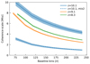 |
Fig. 8. Coherence scales of the mode-mixing foreground GPR components for the three different redshift bins. The baseline dependence of the coherence scale is defined by Equation (10). Based on the estimated values of the θ parameters for the mode-mixing components, the coherence scales range approximately between 8 MHz and ≈2.5 MHz for redshift bins 8.3 (green line) and 9.1 (orange line). For redshift bin 10.1 (blue line), two mode-mixing components are required, yielding coherence scales ranging approximately between 10 MHz and 4 MHz for the first component (solid line), and between 3 MHz and 1 MHz for the second (dashed line). |
The ‘Excess’ component captures small-scale residual structures not fully accounted for by the foreground models. Overall, we observe that the coherence scale of the excess component is consistent across all redshift bins. Compared to the coherence scale observed in LOFAR20, where a coherence scale of 0.26 MHz was found using a Matérn 5/2 kernel, we now find a coherence scale of approximately 0.4 MHz using a radial basis function (RBF) kernel. This indicates that the excess component in our current analysis is overall more frequency coherent. Possible sources of this residual excess are discussed in Section 6.
The ‘21 cm’ component remains largely unconstrained across all redshifts, and its variance is significantly lower than the noise variance. This is expected as we are using a relatively short total integration time. In this paper, we conservatively subtract only the foreground components (‘sky’ and ‘mode-mixing’) from the data. We have not yet attempted to remove the ‘excess’ component (for a discussion on this see e.g. Acharya et al. 2024b), but we may consider doing so in the future, once we are confident that it can be properly separated from the 21 cm signal.
4.2. Power spectra
Figures 9 and 10 present the power spectra of the different components resulting from the ML-GPR decomposition. The foreground components are effectively described by a combination of a spectrally very smooth component and a spectrally less smooth component, both of which are well confined within the wedge region in k-space (see the second row of Figure 9). For small baselines (k⊥ below 0.1 h cMpc−1), the foreground power even falls below the thermal noise level for k∥>0.2 h cMpc−1 at redshifts z≈8.3 and z≈9.1, and for k∥>0.3 h cMpc−1 at z≈10.1. This illustrates the more intense foreground power for the redshift bin z≈10.1.
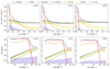 |
Fig. 9. ML-GPR components decomposition of the residual Stokes-I for the three redshift bins. The residual Stokes-I data (blue line) are decomposed into the following components: foreground sky (red), mode-mixing (orange), excess (yellow), noise (green), and the 21 cm signal (magenta). The residual (grey line) represents the Stokes-I data after subtracting all the foreground components. The shaded area represents the 2-σ uncertainty. The top panel displays the cylindrically averaged power spectra as a function of k∥ (averaged over k⊥), while the bottom panels shows the spherically averaged power spectra. |
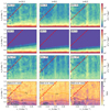 |
Fig. 10. Cylindrically averaged power spectra of the ML-GPR component decomposition of the residual Stokes-I data for the three redshift bins. The top row shows the power spectra before ML-GPR. The second row shows the power spectra of the foreground components only (comprising the ‘sky’ and ‘mode-mixing’ components). The third row presents the power spectra of the residual data after subtracting the foregrounds using ML-GPR. The last row shows the ratio of the residual power to the thermal noise power. In all panels, the foreground horizon line is depicted by a dashed red line. The solid black line in the second row delimits the regions below which the foregrounds power is higher than the thermal noise power. |
The effective confinement of the foreground power within the wedge is crucial for the separability between the foregrounds and the 21 cm signal (Mertens et al. 2018). Our improvements in calibration and RFI mitigation have significantly reduced spectrally correlated contaminants, leading to a better separability of the foregrounds from the 21 cm signal of interest.
The excess component has less spectral coherence than the foreground components. While it exceeds the noise power within the wedge regions, its influence decreases as k∥ increases. Even at high k∥, the excess remains only a small fraction of the noise power, indicating that while the excess component is not entirely negligible, it has a limited impact at higher k∥ modes, particularly above the foreground wedge.
The variance of the 21 cm signal component remains unconstrained across all three redshift bins. Consequently, the power spectra of this component are very low but with large uncertainties, reflecting the large uncertainties in the parameters associated with this component. This behaviour is consistent with the findings of Mertens et al. (2024), where a scenario without a 21 cm signal was tested, resulting in similar uncertainties. The same pattern was also observed by Acharya et al. (2024a) with LOFAR simulation when the 21 cm signal variance was much smaller than the noise variance. This consistency confirms that no 21 cm signal is detected in our data, or at least that it is not captured by the 21 cm component in our analysis.
After subtracting the foreground components from the data (after ML-GPR), the residual power spectra primarily consist of noise and the excess component, and are thus confined to low k∥ modes. On average, the ratio of the residual power spectra to the thermal noise power spectra at high k∥ (above k∥=1 h cMpc−1) is approximately 1.6, 1.4 and 2.2 for the redshift bins z≈10.1,9.1, and 8.3, respectively. At lower k∥ (below k∥=0.2 h cMpc−1), the mean ratios are approximately 5.5, 5.0, and 5.9 for redshifts z≈10.1,9.1, and 8.3, respectively.
The observed ratios are lower for certain k⊥ values where the noise is higher, like k⊥=0.15 h cMpc−1 for example. This is because the ratio is computed relative to the thermal noise, and the excess component does not scale with the thermal noise. As a result, regions with higher noise exhibit lower ratios. On a related note, the higher power observed in Figure 10 (and in Appendix B) before and after ML-GPR around k⊥≈0.15 h cMpc−1 is linked to the lower density of baselines of LOFAR in this range, when observing the NCP, which results in higher noise.
4.3. Comparison with previous results
Our updated analysis demonstrates a significant reduction in residual power across the entire k-range. Figure 11 presents a comparison between the cylindrically averaged power spectra from our LOFAR20 analysis and the current analysis. On average, we observe a reduction in power inside the wedge by a factor of approximately two. In the LOFAR20 analysis, the ratio of residual power to thermal noise was about 6.2 inside the wedge and approximately 3 above it. These ratios have been reduced to about 3 inside the wedge and 1.6 above it in our current analysis.
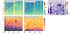 |
Fig. 11. Comparison between the current results and those of LOFAR20 at redshift z≈9.1. The top row shows the residual cylindrically averaged power spectra after GPR for the LOFAR20 dataset (left panel), the current dataset (middle panel), and the ratio between the two (right panel). The bottom row presents the ratio of the residual power to the thermal noise for the LOFAR20 dataset (left panel) and the current dataset (middle panel), accompanied by smoothed contour maps to emphasise the differences. In all panels, the foreground horizon line is indicated by a dashed red line. The significant reduction in residual power across the full k-space demonstrates the effectiveness of our improved data processing techniques. |
Notably, the most substantial reductions – by factors of approximately 4–5 – are observed at k⊥≈0.08 and 0.16 h cMpc−1. These reductions are likely due to residual RFI, with the former being directly associated with local sources that we have effectively mitigated through delay-space baseline flagging techniques.
The application of delay-space baseline flagging (see Section 3.4) has proven effective in reducing excess power on small baselines, which are particularly susceptible to RFI contamination. However, this improvement comes at the expense of an increase in thermal noise. Consequently, while the ratio of residual power to thermal noise has decreased significantly for small baselines, the ratio between the residuals from the LOFAR20 and current analyses remains close to unity in this region.
These improvements are the cumulative result of enhancements implemented at every stage of our analysis: by refining the calibration procedures, improving sky model subtraction, optimising the GPR methodology, and enhancing RFI excision techniques, we have significantly reduced residual power levels using a dataset similar to that used in the LOFAR20 analysis. These methodological advancements have collectively contributed to bringing our measurements closer to the theoretical thermal noise limit. This demonstrates that careful attention to data processing details can lead to substantial improvements, even when using comparable observational data.
4.4. New upper limits
Finally, the noise-bias-subtracted Stokes-I spherically averaged power spectra for each of the three redshift bins (z≈10.1,9.1, and 8.3) was computed to derive upper limits on the 21 cm signal. The power spectra were calculated within seven k-bins, logarithmically spaced between kmin=0.06 h cMpc−1 and kmax=0.5 h cMpc−1, with a bin size of Δk/k≈0.3. This choice of k-bins balances the need for sufficient k-space resolution with the statistical requirements for averaging. The same input dataset for the noise, derived from time-differenced visibilities and used in ML-GPR, was used to compute the power-spectra noise bias,  . This was subtracted from the residual Stokes-I power, after ML-GPR,
  .
.
To estimate the uncertainties and upper limits on the 21 cm power spectrum, we recall that we employed a sampling approach inherent to our ML-GPR framework. Specifically, we generated multiple realisations of the power spectrum by sampling from the posterior distribution of the parameters obtained during the GPR analysis (see Section 3.7). For each realisation, we computed the spherically averaged power spectrum, incorporating the uncertainties from both the parameters and the intrinsic sampling variance. The noise power spectrum, which was subtracted from the residual power spectrum as a bias, has its own uncertainty due to sampling variance, which was also accounted for. This ensemble of power spectra allowed us to construct a distribution for each k-bin, from which we extracted the 95% confidence interval to establish 2-σ uncertainties and upper limits.
The resulting power spectra for the three redshift bins are presented in Figure 12. Our analysis yields the most stringent 2-σ upper limits to date on the 21 cm power spectrum from LOFAR for all three redshift bins. The new upper limits at z≈9.1 represent an improvement by a factor of 2 to 4 compared to the LOFAR20 results, achieved with comparable observational data. The upper limits for z≈8.3 and z≈10.1 also set new benchmarks, expanding the redshift range over which meaningful constraints can be placed on the 21 cm signal.
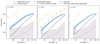 |
Fig. 12. Final spherically averaged power spectra from the combined 10-night dataset, after ML-GPR residual foreground removal and noise bias removal, are shown as the blue line, with the shaded blue area representing the 95% confidence interval. Previous LOFAR upper limits from LOFAR20 (dark orange line) and Patil et al. (2017) (light orange line) are included for comparison. The theoretical thermal noise power spectrum is depicted by the dashed black line, and its 2-σ error is indicated by the dotted line. The new upper limits at z≈9.1 represent an improvement by a factor of 2–4 compared to the LOFAR 2020 results, achieved with comparable observational data. The shaded lavender-grey area represents the 2-σ upper limits that would be obtained if both the ‘excess’ and ‘foreground’ components were subtracted from the data. |
Despite all the improvements, the measured power spectra remain dominated by residual foregrounds and systematics, particularly at low k values. These residuals are primarily due to the excess component identified in our ML-GPR decomposition. Moreover, the residuals are only partially correlated between nights, whereas a true 21 cm signal would be fully correlated (assuming it dominates over the noise), and, to a first order, isotropic (i.e. exhibiting constant power across all modes of a given k). Consequently, we do not interpret the positive values of  as a detection of the 21 cm signal. Instead, we conservatively treat them as upper limits.
The 2-σ upper limits for each k-bin and redshift are reported in Table 3. These limits are derived from the 95% confidence intervals of the sampled power spectra distributions, accounting for both statistical uncertainties and residual systematics in the data. The most stringent 2-σ upper limit is found for the redshift bin z≈9.1, with  at k=0.076 h cMpc−1. Overall, we found that the redshift bin z≈9.1 provided the best upper limits, as it is the cleanest among the three bins analysed. This result is expected due to higher foreground levels at z≈10.1, which complicate the isolation of the 21 cm signal, and lower sensitivity at z≈8.3, caused by increased contamination from RFI at small baselines. The higher RFI contamination leads to a greater flagging fraction of the data at z≈8.3, reducing the effective sensitivity (see Figure 4). Nevertheless, the availability of upper limits across three distinct redshift bins enhances our ability to constrain astrophysical parameters related to the EoR, which we shall present in an accompanying paper (Ghara et al. 2025).
 upper limits at the 2-σ level (
 ) and the residual power after GPR minus the noise power (
 ) from the 10-night dataset, at given k bins for the three redshift ranges.
Following the approach of Acharya et al. (2024b), we investigated the potential improvement in the upper limits if we could cleanly isolate the ‘excess’ component from the 21 cm signal component and subtract it from the data. The spherically averaged power spectra resulting from this hypothetical subtraction are depicted as the shaded lavender-grey area in Figure 12. This would yield a best 2-σ upper limit at z≈9.1 of  at k=0.076 h cMpc−1. However, given our current inability to fully separate the ‘excess’ component from the 21 cm signal component, we have decided, as in LOFAR20, to conservatively include the ‘excess’ component in the final results.
Recent results from other experiments provide useful context for interpreting our new limits. The best published MWA upper limit,  at z≈6.5 and k=0.15 h cMpc−1 (Trott et al. 2020), lies at a lower redshift than the LOFAR measurements presented here. The most recent HERA upper limits (HERA Collaboration 2023), by contrast, overlap more directly in redshift. At z≈7.9, HERA reports a 2-σ upper limit of
  at k=0.34 h cMpc−1, which is significantly lower than our LOFAR limit at z≈8.3, measured at a lower k-mode. At z≈10.4, HERA obtains a limit of
  at k=0.36 h cMpc−1, which is comparable to our result of
 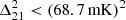 at z≈10.1, again at a lower k-mode.
5. Data analysis validations
Ensuring the integrity of the 21 cm signal throughout our data processing pipeline is a major concern. Given the faintness of the expected 21 cm signal and the overwhelming presence of foregrounds and instrumental effects, each step in the pipeline has the potential to inadvertently suppress or bias the 21 cm signal. In this section, we present the validation procedures applied to critical components of our pipeline.
5.1. Signal retention during calibration
The intensity scale of the visibilities, and hence ultimately the 21 cm signal strength, was fixed during the DI-calibration step. The absolute intensity scale of the sky model was set using the same procedure as described in LOFAR20, using the flat-spectrum source NVSSJ011732+892848 (RA01h,17m,33s, Dec +89°,28′,49″ in J2000) with an intrinsic flux of 8.1 Jy with 5% accuracy (Patil et al. 2017). The accuracy of our flux scale calibration was previously tested in LOFAR20 by cross-identifying the brightest sources within 3° of the phase centre with the 6C and 7C 151 MHz radio catalogues (Baldwin et al. 1985; Hales et al. 2007), confirming the reliability of our calibration. Since our DI-calibration procedure is not fundamentally changed, we refer the reader to LOFAR20 for more detailed validation results of this step.
When subtracting the sky-model multiplied with the DD calibrated gains, there is a risk of signal suppression. Sardarabadi & Koopmans (2019) and Mevius et al. (2022) investigated the effect of DD-calibration and sky-model subtraction on signal suppression and residual noise in the power spectrum. Using the spectral smoothness constraint as implemented in Sagecal-CO (Yatawatta 2015), overfitting and therefore signal suppression is significantly reduced. It was found that no signal suppression occurs if the baselines used in the power spectrum – those <250λ – are excluded from the calibration step. Excluding baselines from the calibration will result in extra noise on those baselines due to overfitting13. However, the current smoothness constraint settings in Sagecal-CO significantly reduce this additional noise. Brackenhoff et al. (2024) have shown that additional ionospheric noise can also be mitigated using this method.
Signal suppression due to DI-calibration is expected to be negligible, as no visibility subtraction is involved in this step. This justifies the broader baseline selection between 50 and 5000 λ at this stage. However, calibration errors caused by unmodelled sources and overfitting during DI-calibration can still result in additional noise (Höfer et al. 2025). This noise cannot be removed later in the calibration chain because the visibilities are multiplied by the inverse calibration gains. This effect is mitigated by minimising the number of free parameters, as we currently do by starting with a high time resolution, spectrally smooth calibration, followed by a 4-hour long time interval bandpass calibration.
We conclude that excluding short baselines from the calibration process prevents suppression of the 21 cm signal. A slight increase in variance may result from the transfer of minor gain errors from longer to shorter baselines. Nevertheless, this effect is expected to be minimal due to regularisation, as is shown by Sardarabadi & Koopmans (2019), Mevius et al. (2022).
5.2. Signal retention during RFI flagging
In order to verify that the post-calibration flagging steps (described in Sect. 3.4) would not suppress a 21 cm signal, we injected an artificial signal in the residual visibilities of one of the observations. The power spectra after flagging with and without injected signal were subtracted to obtain a measure of the recovered signal. This was then compared to the power spectrum of the injected signal. Figure 13 shows that the injected signal is recovered well, both after the wide-field AOFlagger step and after the visibility flagging. The small changes, all within the 1-σ errors, between the injected and recovered signal are due to slight variations in the visibility standard deviation, which cause slightly different time and frequency bins to be flagged when a 21 cm signal is present. As expected, this effect decreases with decreasing amplitude of the injected signal. In order to be able to test the recovery of the injected signal over the thermal noise, we injected a signal with an amplitude larger than expected for any real 21 cm signal. We therefore conclude that the post-calibration flagging does not have a significant effect on recovery of the 21 cm signal.
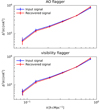 |
Fig. 13. Recovery test of injected 21 cm signal, validating the post-processing flagging step. Top: effect after applying AOFlagger. Bottom: effect of the visibility flagging step. The difference between injected and recovered signal is within the 1 sigma uncertainty. |
5.3. Signal retention during residual foregrounds removal
The ML-GPR algorithm is a powerful tool for foreground mitigation, but it may inadvertently alter the recovered 21 cm signal. Assessing the impact of ML-GPR on the 21 cm signal is therefore essential to ensure the reliability of our results. To this end, we performed signal injection tests, similar to those in LOFAR20, though here we employed a much more realistic and broader set of possible 21 cm signals.
Synthetic 21 cm signals were added to the data just before the ML-GPR step. The signals were generated using the decoder of the trained VAE kernel, which allowed us to produce a variety of power spectra corresponding to different points in the latent space of the VAE model. We selected 25 different shapes of the 21 cm power spectrum by choosing points that cover the full distribution of the training points in the latent space. This sampling captures a wide range of possible 21 cm signal shapes as represented by the Grizzly simulations used to train the VAE kernel. For each of these 25 shapes, we scaled the power to be equal to 0.25, 0.5, 1.0, and 2 times the noise power, resulting in 100 different injected signals that cover a broad range of signal strengths. We repeated this exercise with synthetic 21 cm signals generated using a VAE kernel trained with 21cmFAST simulations, while still using the Grizzly trained VAE kernel in ML-GPR. This ensures that the injection test is not dependent on the training set of the VAE kernel.
For each injected signal, we generated a realisation of a visibility cube which has the desired power spectrum and add it to the data before ML-GPR. ML-GPR was then performed on this data cube with the injected signal, using the same priors as were used for the actual data without injection. The residual power spectrum of the data without an injected signal was subtracted from the residual power spectrum obtained after ML-GPR on the data with the injected signal. This difference yields the recovered 21 cm power spectrum, which can be compared to the power spectrum of the injected signal to assess any potential absorption or biasing caused by ML-GPR.
To quantify the performance of ML-GPR in recovering the injected 21 cm signal, we calculated a p value for each k-bin, defined as the fraction of realisations where the residual power spectrum is higher than the injected power spectrum. We then derived the z-score using the inverse cumulative distribution function of the normal distribution. A z-score indicates the number of standard deviations by which the recovered 21 cm signal deviates from the injected 21 cm signal. A negative z-score suggests absorption of the signal, with values below −2 indicating absorption beyond the 2-σ upper limits.
The z-scores for all signal injection tests are shown in the top panels of Figure 14 for the Grizzly simulation sets and Figure 15 for the 21cmFAST simulation set, with different intensities of the injected signal denoted by different colours. For the Grizzly simulation set, only one case (out of 100 cases) presents a few k-bin just below a z-score of −2 for the redshift bin z≈8.3, none for z≈9.1, and only four cases for z≈10.1. For the 21cmFAST simulation set, four cases present a few k-bin just below a z-score of −2 for the redshift bin z≈8.3, one for z≈9.1, and 11 for z≈10.1. The lower panels of Figures 14 and 15 show the power spectra of the injected signal, with the colour indicating the mean z-score for each case. The cases with the worst recovery are those characterised by a flat power spectrum or an upturn at large scales. These cases are particularly challenging to recover as the frequency coherence scale is closer to that of the mode-mixing component. Nevertheless, ML-GPR performs remarkably well even in these challenging cases. An additional point supporting the robustness of our analysis is that, in all injection cases, the variance parameter of the 21 cm signal component ( ) was consistently constrained, whereas it remains unconstrained in the actual data. This indicates that if a 21 cm signal were present above the noise level, it would indeed be detected and constrained by our ML-GPR model.
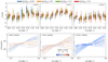 |
Fig. 14. Results of the injection test, validating the ML-GPR residual foreground removal step, with the Grizzly simulations. The top plots show the z-score as a function of k-mode. A total of 25 synthetic 21 cm signals are tested, each with four different intensities. Each box-plot represents the distribution of z-scores for all 25 cases, with different box-plot colours indicating different signal intensities. The central line represents the median z-score, the box edges indicate the 25th and 75th percentiles (interquartile range), the whiskers extend to the data points within 1.5 times the interquartile range, and individual points beyond the whiskers represent outliers. A negative z-score suggests absorption of the signal, with values below −2 indicating absorption beyond the 2-σ upper limits. The bottom panel shows the spherically averaged power spectrum (for |

Our signal injection tests demonstrate that ML-GPR does not significantly suppress the 21 cm signal. The recovered power spectra match the injected signals within the uncertainties for almost all cases, confirming the reliability of ML-GPR in our analysis. Over the 600 injections that we performed (three redshift bins, two simulation codes), only 3.5% presented a z-score below −2. We also note that the z-score for the smallest k-bins was consistently above −2, indicating a robust recovery for the larger spatial scales. When considering individual k-bins, only 1.1% of the bins exhibited a z-score below −2. This validation shows that our ML-GPR pipeline preserves the 21 cm signal while effectively mitigating foregrounds and systematics. Furthermore, these results indicate that any potential bias in the 21 cm power spectrum is minimal and does not necessitate correction, thereby supporting the robustness of our analysis.
6. Discussion
Throughout the reprocessing of the LOFAR observations originally analysed in LOFAR20, we have significantly enhanced our data processing pipeline. Each step was carefully reviewed and refined to minimise sources of excess power that hinder the detection of the 21 cm signal. In this section, we review the changes made to the pipeline and how they contribute to the overall improvement, examine the sources of remaining excess power, and discuss further developments needed to enhance the quality of our results.
6.1. Quantifying pipeline improvements
Several key updates to the pipeline contributed to the reduction of excess variance across the dataset. The revised DI-calibration scheme, which separates spectral and temporal components, led to a modest reduction in excess variance of about 10–20%. More importantly, it reduced gain error by two to three orders of magnitude, making the calibration significantly more robust. The updated DD-calibration, particularly the removal of some source clusters beyond the first beam null, reduced foreground contamination within the wedge by up to a factor of five for some nights. However, the level of improvement varied with both night and observed LST range, leading to a more modest average reduction – closer to a factor of two or less on the combined dataset. Enhanced RFI flagging after calibration reduced power by up to a factor of 10 on short baselines in some cases, though night-to-night variability means the average improvement is closer to a factor of 4–5. Finally, the refinement of the foreground removal algorithm using ML-GPR played a key role in further reducing the final excess variance. Its effectiveness was supported by the improved calibration and RFI flagging, which helped confine foreground power to the low k∥ range. This improved the separation between foregrounds and residual (excess and 21 cm) components, making the foreground removal process more efficient and reliable.
6.2. Sources of excess
We investigated many sources of excess power during this reprocessing:
Bright sources in the side-lobes – Bright sources, far outside the primary beam, such as Cas A and Cygnus A present significant challenges. Gan et al. (2022) identified them as a source of excess variance in the LOFAR20 results. During observations, the LOFAR station beam gain in their direction evolves considerably. The deep nulls and strong spectral variations in the sidelobes of the beam, resulting from the regular structure of the array, paired with beam modelling errors, make subtracting these sources during DD-calibration very difficult, especially since we impose spectrally smooth solutions. Any residual flux from these sources introduces spectral fluctuations into the data. Additionally, Munshi et al. (2024) showed that bright distant sources can contribute power at much higher k∥ than previously thought. Currently, only Cas A and Cygnus A are addressed, while many other sources, such as Taurus A, Virgo A, and other bright 3C sources, may impact our data as well. This is clearly a source of excess power. Although improvements in the Cas A and Cygnus A sky models and directional post-calibration flagging helped reduce their impact, much work remains to be done to further mitigate their impact (Ceccotti et al. 2025a). Optimising calibration and flagging (or avoidance) strategies for bright sources in the sidelobes is one of the major topics currently under study.
DD-calibration errors – Enforcing spectrally smooth solutions for DD-calibration has significantly reduced excess variance due to calibration errors. However, related to the point above, we noticed that calibrating and subtracting clusters of sources located far beyond the first null of the beam may in some circumstances do more harm than good. In current analysis, removing those clusters from the sky model improved the final 21 cm signal power spectrum limit. Deciding which sources to include in the final sky model, however, requires further investigation and automation.
DI-calibration errors – Improving DI-calibration was a major focus of this reprocessing, and we managed to considerably reduce the gain errors in this step. The number of free parameters in DI-calibration was significantly reduced by allowing only a time-stable but spectrally varying bandpass gain, and conversely applying time-varying but spectrally smooth solutions to the visibilities. This approach minimises the impact of DI-calibration errors on the power spectra, particularly at higher delays. We believe DI-calibration errors to not be a significant source of excess power anymore. This will be further quantified by (Höfer et al. 2025).
Radio frequency interference – In the reprocessing, we observed the significant impact that low-level RFI can have on the power spectra (see e.g. Figure 4); it was clearly a source of excess power. Broadband RFI can introduce frequency structure at high k∥ and is usually difficult to detect and flag. Processing observations targeting 3C 196, for example, showed that, for targets other than the NCP where RFI does not coherently add up, the excess is reduced (Ceccotti et al. 2025b). While major improvements were implemented in the pipeline to reduce the impact of RFI, which have clearly been effective, further work is needed: our current approach, which discards any data – even entire baselines – affected by RFI, has the negative effect of decreasing our sensitivity. This is especially the case for small baselines, which are heavily affected by local sources of RFI, thereby reducing our sensitivity at the largest scales.
Ionosphere errors – In a recent paper by Brackenhoff et al. (2024) it is shown that calibration errors induced by ionospheric disturbances are unlikely to be the cause of excess variance. Gan et al. (2022) also did not observe any correlation between metrics assessing ionospheric activity and excess variance in the observations. However, the interaction of ionospheric errors with other effects, such as beam errors in the far sidelobes, requires further investigation.
6.3. Future improvement
Figure 16 effectively illustrates the improvements achieved in our processing pipeline to reduce the aforementioned sources of excess power, as well as highlighting areas that still require attention. The figure shows the night-to-night cross-coherence for different regions of the cylindrically averaged power spectra, evaluated over all pairs of nights and across the three redshift bins. We split the cylindrically averaged power-spectra into four regions, corresponding different angular ranges: (i) the region covered by our NCP sky model (<15°, in yellow), (ii) the region where we expect most of the power from the bright sources Cas A and Cygnus A (15°–50°, in green), (iii) the foreground wedge region affected by more distant bright sources (>50°, light blue), and (iv) the EoR window (dark blue). Compared to the results from LOFAR20 (indicated by the dashed line in the top-middle panel), we observe a considerable reduction in night-to-night correlation across all k-space regions. Specifically, the correlation in the EoR window and in the foreground wedge above 50° is now very close to zero, indicating minimal remaining coherent excess power in these regions. However, some correlation remains in the foreground wedge within the 15°–50° range, suggesting that distant and bright sources continue to contribute a coherent excess. Additionally, significant correlation persists in the foreground wedge below 15°, pointing to contributions from sources within the first few sidelobes of the LOFAR station beam. The fact that the night-to-night correlation decreases considerably when the two nights are observed at very different local sidereal times – and thus see the sky through a very different primary beam – as shown in the lower panel of Figure 16, indicates that these residual excesses have a sky origin.
 |
Fig. 16. Night-to-night cross-coherence for different regions of the cylindrically averaged power spectra, evaluated over all pairs of nights and across the three redshift bins. The top panels display density plots of the cross-coherence values, with colours indicating different regions of the power spectra (the specific regions are illustrated in the insets). The bottom panels present the individual cross-coherence values as a function of Local Sidereal Times (LST) time difference, along with a fitted trend line to highlight the overall pattern. For the redshift bin at z≈9.1 (middle panel), we also include in a dashed line the cross-coherence results from LOFAR20 for comparison. |
Most of the causes of excess power, we currently believe, could be mitigated by further improving the calibration scheme, our sky model, and the GPR covariance model. Enhancing our RFI mitigation strategy could also help us to preserve our sensitivity at a large scale.
Further improving the low-level RFI flagging – A possibility under investigation is to use a more specific filtering instead of flagging full baselines. As some of the strong sources of RFI identified in this work are often located near the superterp, a procedure similar to a DD-calibration, but for a source on the ground, could be envisaged (Finlay et al. 2023). A similar method is also investigated for the NenuFAR data (Munshi et al. 2025a).
Improving the GPR covariance model – The separation between residual foregrounds and the 21 cm signal remains a significant challenge in our analysis. Further enhancements to our ML-GPR framework are necessary to address this issue. Our strategy has been to refine the covariance model to better match the actual covariance of the data. This approach was successfully applied to the 21 cm signal component by implementing learned kernels trained on 21 cm simulations. A similar methodology needs to be adopted for the foreground covariance model, which currently relies on a generic covariance function. Developing an analytically defined or simulation-based learned foreground covariance model that incorporates instrumental and systematic effects should greatly enhance the accuracy of our foreground modelling. Additionally, extending the ML-GPR framework to enable a joint analysis over multiple redshifts simultaneously – thereby encompassing a wider bandwidth – could improve our ability to distinguish between the evolving 21 cm signal and the spectrally smooth foregrounds. Implementing this strategy would require our calibration scheme to be executed consistently over the combined redshift bins.
Beam model and calibration – For computational reasons, the beam model is until now not used in DD-calibration. Yet, we see that a major source of excess noise is related to beam effects outside the first null of the beam. Mitigating beam effects in DD-calibration will be a major focus of future improvements to our calibration scheme. This can be accomplished by smart weighting schemes that down weight the effects of nulls in the beam (Brackenhoff et al. 2025) or reducing the number of degrees of freedom by spatial constraints as discussed in Yatawatta (2022). Other ways of reducing the number of degrees of freedom in DD-calibration involve decomposing the calibration in steps that are physically motivated, such as ionospheric effects.
Improving the NCP sky model – In the current analysis, we discarded some of the outer source clusters that were previously used in the NCP sky model, because keeping them in the model would only add to the excess noise, at least for the observations we checked. This evaluation needs to be performed more rigorously. The number of clusters and components in the sky model should be revisited and possibly reduced. At the same time, we notice that bright sources that may have a low apparent brightness when integrated over the full 12 hr observations can cause issues at certain sidereal times when they are in the sidelobes of some of the beams. Therefore, we should investigate the effect of adding more bright sources other than Cas A and Cygnus A.
7. Summary and conclusion
We have presented new upper limits on the 21 cm signal from the EoR, derived from reprocessed LOFAR observations. Building upon the work of LOFAR20, we have significantly enhanced our data processing pipeline and extended our analysis to a broader frequency range, allowing us to set upper limits at redshifts z≈10.1,9.1, and 8.3. The main conclusions of our work are:
-
1.
By significantly modifying our DI-calibration strategy, splitting the spectral and temporal calibration parts, a reduction in gain errors by two to three orders of magnitude was achieved by significantly reducing the number of free parameters. This minimised the impact of DI-calibration errors on the power spectra, particularly at higher delays, effectively eliminating them as a source of excess power.
-
2.
We updated our sky model, incorporating improved models of distant bright sources like Cas A and Cygnus A, which are known to introduce excess variance due to their complex beam interactions. Despite these improvements, residual contributions from these and other bright sources outside the primary beam remain significant sources of excess power. In addition, we found that calibrating and subtracting clusters of sources located far beyond the first null of the beam sometimes increased errors. By removing these distant clusters from the sky model, we improved the final 21 cm signal power spectrum limit.
-
3.
By implementing a new post-calibration RFI mitigation strategy, including delay-space baseline flagging, we significantly reduce excess power caused by low-level and broadband RFI, particularly from local sources. This approach effectively mitigates RFI contamination on small baselines, leading to reductions in power by factors of 4 to 5 at specific k⊥ values. While this leads to increased thermal noise on large scale due to data loss from flagging entire baselines, the overall benefit in reducing RFI-induced excess power far outweighs the sensitivity loss, enhancing the quality of our power spectrum measurements.
-
4.
The GPR method was enhanced by employing a machine learning approach to construct a physically motivated covariance function for the 21 cm signal, thereby improving the separation between the 21 cm signal and foreground components. Additionally, we refined the foreground covariance model by making the coherence scale dependent on baseline length, effectively accounting for the foreground ‘wedge’ in k-space. These advancements substantially improved our ability to isolate the 21 cm signal from foreground contamination.
-
5.
The cumulative effect of all these improvements is a significant reduction of residual power across the entire k-range, effectively minimising systematics in our data. At the redshift bin z≈9.1, residual power inside the wedge decreased by a factor of about two compared to our previous analysis. Specifically, the ratio of residual power to thermal noise decreased from 6.2 to 3 inside the wedge, and from approximately 3 to 1.6 outside it. These advancements bring our measurements closer to the theoretical thermal noise limit, thereby improving the sensitivity of our observations.
-
6.
We have established the most stringent 2-σ upper limits on the 21 cm signal from LOFAR at redshifts z≈10.1,9.1, and 8.3. Specifically, at z≈9.1, we achieved a two- to fourfold improvement over our previous results LOFAR20 using comparable observational data, setting a best upper limit of
 at k=0.076 h cMpc−1. For the other redshifts, we achieved a best upper limit of
  at k=0.076 h cMpc−1 for z≈10.1 and
  at k=0.083 h cMpc−1 for z≈8.3. The upper limits for each k-bin and redshift are reported in Table 3. These upper limits have been rigorously validated through comprehensive tests, including signal injection, ensuring that our data processing and analysis methods do not suppress the 21 cm signal.
These new multi-redshift upper limits provide new constraints that can be used to refine our understanding of the astrophysical processes during the EoR. The implications of these multi-redshift 21 cm signal power spectrum upper limits are presented in an accompanying paper by Ghara et al. (2025). The study uses a Bayesian inference framework based on the 21 cm signal power spectrum modelling using Grizzly code to constrain the IGM properties of the disfavoured reionisation scenarios between redshift 8–10. The study shows that the disfavoured models are still extreme types in which the 21 cm signal fluctuations are mainly driven by rare and large ionised regions. For a standard cosmology scenario without any excess radio background to the CMB, the 95% credible intervals of the disfavoured models at redshift 9.1 represent disfavoured IGM states with averaged ionisation and heated fraction below ≲0.55, an average gas temperature of ≲21 K, and heated region that has a characteristic size of ≲40 Mpc. These constraints are based on uniform priors of the Grizzly source parameters on their ranges and by using conservative limits on the maximum ionisation fraction at those three redshifts, estimated from the CMB Thomson scattering optical depth from Planck. We refer to Ghara et al. (2025) for the detailed constraints on the source and IGM parameters for all three redshifts.
While we have not yet detected the 21 cm signal, the significant improvements achieved in this work lay the groundwork for future analyses with much longer (∼1000 hours) integrations and more advanced data processing techniques. Continued development in RFI mitigation, calibration strategies, beam modelling, and sky modelling will further enhance our ability to detect the elusive 21 cm signal from the EoR.
Data availability
The data underlying this article will be shared on reasonable request to the corresponding author.
Acknowledgments
We are grateful to the referee for their valuable feedback and suggestions that improved this paper. FGM acknowledges the financial support of the PSL Fellowship Programme. LVEK, SAB, KC, SG, CH and SM acknowledge the financial support from the European Research Council (ERC) under the European Union's Horizon 2020 research and innovation programme (Grant agreement No. 884760, ‘CoDEX’). EC (INAF) would like to acknowledge support from the Centre for Data Science and Systems Complexity (DSSC), Faculty of Science and Engineering at the University of Groningen, and from the Ministry of Universities and Research (MUR) through the PRIN project ‘Optimal inference from radio images of the epoch of reionisation’. GM is supported by Swedish Research Council grant 2020-04691. QM acknowledges the financial support of the National Natural Science Foundation of China (Grant No. 12263002). RG acknowledges support from SERB, DST Ramanujan Fellowship no. RJF/2022/000141. EC (Nottingham) acknowledges the support of a Royal Society Dorothy Hodgkin Fellowship and a Royal Society Enhancement Award. SKG is supported by NWO grant number OCENW.M.22.307.
LOw-Frequency ARray, http://www.lofar.org
Murchison Widefield Array, http://www.mwatelescope.org
New Extension in Nançay Upgrading LOFAR, https://nenufar.obs-nancay.fr/en/homepage-en/
Hydrogen Epoch of Reionization Array, https://reionization.org/
Giant Metrewave Radio Telescope, http://www.gmrt.ncra.tifr.res.in
Square Kilometre Array Observatory, https://www.skao.int
These higher-frequency spectral features are unphysical and therefore could overfit the data.
The Superterp consists of 24 densely packed stations within a 300-metre diameter area at the core of LOFAR.
Currently, our GP model does not include spatial (in the plane of the sky) correlation, this is left for a future development.
Although the 21 cm power spectrum is expected to present slight anisotropies due to redshift space distortions and light cone effects, it is common practice to ignore these to the first order and use the spherically averaged power spectrum.
Overfitting occurs on the longer baselines and those errors are transferred to the baselines not used during calibration.
References
- Acharya, A., Mertens, F., Ciardi, B., et al. 2024a, MNRAS, 527, 7835 [Google Scholar]
- Acharya, A., Mertens, F., Ciardi, B., et al. 2024b, MNRAS, 534, L30 [Google Scholar]
- Arrabal Haro, P., Dickinson, M., Finkelstein, S. L., et al. 2023, Nature, 622, 707 [NASA ADS] [CrossRef] [Google Scholar]
- Atek, H., Shuntov, M., Furtak, L. J., et al. 2023, MNRAS, 519, 1201 [Google Scholar]
- Baldwin, J. E., Boysen, R. C., Hales, S. E. G., et al. 1985, MNRAS, 217, 717 [NASA ADS] [Google Scholar]
- Bañados, E., Venemans, B. P., Mazzucchelli, C., et al. 2018, Nature, 553, 473 [Google Scholar]
- Barkana, R. 2018, Nature, 555, 71 [Google Scholar]
- Barkana, R., & Loeb, A. 2001, Phys. Rep., 349, 125 [NASA ADS] [CrossRef] [Google Scholar]
- Barry, N., Hazelton, B., Sullivan, I., Morales, M. F., & Pober, J. C. 2016, MNRAS, 461, 3135 [CrossRef] [Google Scholar]
- Beardsley, A. P., Hazelton, B. J., Sullivan, I. S., et al. 2016, ApJ, 833, 102 [NASA ADS] [CrossRef] [Google Scholar]
- Becker, R. H., Fan, X., White, R. L., et al. 2001, AJ, 122, 2850 [NASA ADS] [CrossRef] [Google Scholar]
- Becker, G. D., Bolton, J. S., Madau, P., et al. 2015, MNRAS, 447, 3402 [Google Scholar]
- Bonaldi, A., Hartley, P., Braun, R., et al. 2025, MNRAS, submitted [arXiv:2503.11740] [Google Scholar]
- Bosman, S. E. I., Fan, X., Jiang, L., et al. 2018, MNRAS, 479, 1055 [Google Scholar]
- Bouwens, R. J., Stefanon, M., Brammer, G., et al. 2023, MNRAS, 523, 1036 [NASA ADS] [CrossRef] [Google Scholar]
- Boylan-Kolchin, M. 2023, Nat. Astron., 7, 731 [NASA ADS] [CrossRef] [Google Scholar]
- Brackenhoff, S. A., Mevius, M., Koopmans, L. V. E., et al. 2024, MNRAS, 533, 632 [NASA ADS] [CrossRef] [Google Scholar]
- Brackenhoff, S. A., Offringa, A. R., Mevius, M., et al. 2025, MNRAS, submitted [arXiv:2504.02483] [Google Scholar]
- Buchner, J. 2021, J. Open Source Softw., 6, 3001 [CrossRef] [Google Scholar]
- Ceccotti, E., Offringa, A. R., Koopmans, L. V., et al. 2023, MNRAS, 525, 3946 [NASA ADS] [Google Scholar]
- Ceccotti, E., Offringa, A. R., Koopmans, L. V. E., et al. 2025a, A&A, 696, A56 [NASA ADS] [CrossRef] [EDP Sciences] [Google Scholar]
- Ceccotti, E., Offringa, A. R., Mertens, F. G., et al. 2025b, MNRAS, submitted [arXiv:2504.18534] [Google Scholar]
- Chokshi, A., Barry, N., Line, J. L. B., et al. 2024, MNRAS, 534, 2475 [Google Scholar]
- Ciardi, B., & Ferrara, A. 2005, Space Sci. Rev., 116, 625 [Google Scholar]
- Datta, A., Bowman, J. D., & Carilli, C. L. 2010, ApJ, 724, 526 [NASA ADS] [CrossRef] [Google Scholar]
- Datta, K. K., Mellema, G., Mao, Y., et al. 2012, MNRAS, 424, 1877 [NASA ADS] [CrossRef] [Google Scholar]
- Davies, F. B., Hennawi, J. F., Bañados, E., et al. 2018, ApJ, 864, 142 [NASA ADS] [CrossRef] [Google Scholar]
- Deboer, D. R., Parsons, A. R., Aguirre, J. E., et al. 2017, PASP, 129, 45001 [Google Scholar]
- de Bruyn, A. G. 2012, Am. Astron. Soc. Meet. Abstr., 219, 214.05 [Google Scholar]
- Donnan, C. T., McLeod, D. J., Dunlop, J. S., et al. 2023, MNRAS, 518, 6011 [Google Scholar]
- Eilers, A. -C., Davies, F. B., & Hennawi, J. F. 2018, ApJ, 864, 53 [NASA ADS] [CrossRef] [Google Scholar]
- Ewall-Wice, A., Dillon, J. S., Liu, A., & Hewitt, J. 2017, MNRAS, 470, 1849 [CrossRef] [Google Scholar]
- Fan, X., Strauss, M. A., Richards, G. T., et al. 2006, AJ, 131, 1203 [NASA ADS] [CrossRef] [Google Scholar]
- Fialkov, A., & Barkana, R. 2019, MNRAS, 486, 1763 [NASA ADS] [CrossRef] [Google Scholar]
- Finkelstein, S. L., Leung, G. C. K., Bagley, M. B., et al. 2024, ApJ, 969, L2 [NASA ADS] [CrossRef] [Google Scholar]
- Finlay, C., Bassett, B. A., Kunz, M., & Oozeer, N. 2023, MNRAS, 524, 3231 [Google Scholar]
- Furlanetto, S. R. 2016, in Understanding the Epoch of Cosmic Reionization: Challenges and Progress, eds. A. Mesinger (Springer International Publishing), 423, 247 [Google Scholar]
- Furlanetto, S. R., Oh, S. P., & Briggs, F. H. 2006, Phys. Rep., 433, 181 [Google Scholar]
- Gan, H., Koopmans, L. V., Mertens, F. G., et al. 2022, A&A, 663, A9 [NASA ADS] [CrossRef] [EDP Sciences] [Google Scholar]
- Gan, H., Mertens, F. G., Koopmans, L. V., et al. 2023, A&A, 669, A20 [NASA ADS] [CrossRef] [EDP Sciences] [Google Scholar]
- Gehlot, B. K., Jacobs, D. C., Bowman, J. D., et al. 2021, MNRAS, 506, 4578 [NASA ADS] [CrossRef] [Google Scholar]
- Ghara, R., Choudhury, T. R., & Datta, K. K. 2015, MNRAS, 447, 1806 [NASA ADS] [CrossRef] [Google Scholar]
- Ghara, R., Mellema, G., Giri, S. K., et al. 2018, MNRAS, 476, 1741 [NASA ADS] [CrossRef] [Google Scholar]
- Ghara, R., Giri, S. K., Mellema, G., et al. 2020, MNRAS, 493, 4728 [NASA ADS] [CrossRef] [Google Scholar]
- Ghara, R., Zaroubi, S., Ciardi, B., et al. 2025, A&A, in press https://doi.org/10.1051/0004-6361/202554163 [Google Scholar]
- Greig, B., Mesinger, A., Haiman, Z., & Simcoe, R. A. 2017, MNRAS, 466, 4239 [Google Scholar]
- Greig, B., Mesinger, A., Koopmans, L. V., et al. 2021, MNRAS, 501, 1 [Google Scholar]
- Gupta, Y., Ajithkumar, B., Kale, H. S., et al. 2017, Curr. Sci., 113, 707 [NASA ADS] [CrossRef] [Google Scholar]
- Hales, S. E., Riley, J. M., Waldram, E. M., Warner, P. J., & Baldwin, J. E. 2007, MNRAS, 382, 1639 [Google Scholar]
- Harikane, Y., Zhang, Y., Nakajima, K., et al. 2023, ApJ, 959, 39 [NASA ADS] [CrossRef] [Google Scholar]
- HERA Collaboration (Abdurashidova, Z., et al.) 2023, ApJ, 945, 124 [NASA ADS] [CrossRef] [Google Scholar]
- Höfer, C., Koopmans, L. V. E., Brackenhoff, S. A., et al. 2025, A&A, submitted [arXiv:2504.03554] [Google Scholar]
- Hothi, I., Chapman, E., Pritchard, J. R., et al. 2021, MNRAS, 500, 2264 [Google Scholar]
- Jelić, V., Zaroubi, S., Labropoulos, P., et al. 2008, MNRAS, 389, 1319 [CrossRef] [Google Scholar]
- Jelić, V., Zaroubi, S., Labropoulos, P., et al. 2010, MNRAS, 409, 1647 [CrossRef] [Google Scholar]
- Jordan, C. H., Murray, S., Trott, C. M., et al. 2017, MNRAS, 471, 3974 [NASA ADS] [CrossRef] [Google Scholar]
- Keating, L. C., Weinberger, L. H., Kulkarni, G., et al. 2020, MNRAS, 491, 1736 [NASA ADS] [CrossRef] [Google Scholar]
- Kern, N. S., & Liu, A. 2021, MNRAS, 501, 1463 [Google Scholar]
- Kern, N. S., Parsons, A. R., Dillon, J. S., et al. 2020, ApJ, 888, 70 [NASA ADS] [CrossRef] [Google Scholar]
- Kolopanis, M., Pober, J. C., Jacobs, D. C., & McGraw, S. 2023, MNRAS, 521, 5120 [NASA ADS] [Google Scholar]
- Koopmans, L. V. 2010, ApJ, 718, 963 [NASA ADS] [CrossRef] [Google Scholar]
- Koopmans, L., Pritchard, J., Mellema, G., et al. 2015, Proceedings of Advancing Astrophysics with the Square Kilometre Array (AASKA14), http://pos.sissa.it/cgi-bin/reader/conf.cgi?confid=215, 1 [Google Scholar]
- Liu, A., Parsons, A. R., & Trott, C. M. 2014, Phys. Rev. D - Part. Fields Grav. Cosmol., 90, 23019 [Google Scholar]
- Loeb, A., & Furlanetto, S. R. 2013, The First Galaxies in the Universe, 1 [Google Scholar]
- Mason, C. A., Trenti, M., & Treu, T. 2023, MNRAS, 521, 497 [NASA ADS] [CrossRef] [Google Scholar]
- Mellema, G., Koopmans, L., Shukla, H., et al. 2015, Proceedings of Advancing Astrophysics with the Square Kilometre Array (AASKA14), http://pos.sissa.it/cgi-bin/reader/conf.cgi?confid=215, 10 [Google Scholar]
- Mertens, F. G., Ghosh, A., & Koopmans, L. V. 2018, MNRAS, 478, 3640 [NASA ADS] [Google Scholar]
- Mertens, F. G. G., Mevius, M., Koopmans, L. V. E. V., et al. 2020, MNRAS, 493, 1662 [NASA ADS] [CrossRef] [Google Scholar]
- Mertens, F. G., Bobin, J., & Carucci, I. P. 2024, MNRAS, 527, 3517 [Google Scholar]
- Mevius, M., van der Tol, S., Pandey, V. N., et al. 2016, Radio Sci., 51, 927 [Google Scholar]
- Mevius, M., Mertens, F., Koopmans, L. V., et al. 2022, MNRAS, 509, 3693 [Google Scholar]
- Mondal, R., Fialkov, A., Fling, C., et al. 2020, MNRAS, 498, 4178 [NASA ADS] [CrossRef] [Google Scholar]
- Morales, M. F., & Wyithe, J. S. B. 2010, ARA&A, 48, 127 [NASA ADS] [CrossRef] [Google Scholar]
- Morales, M. F., Bowman, J. D., & Hewitt, J. N. 2006, ApJ, 648, 767 [NASA ADS] [CrossRef] [Google Scholar]
- Morales, M. F., Hazelton, B., Sullivan, I., & Beardsley, A. 2012, ApJ, 752, 137 [NASA ADS] [CrossRef] [Google Scholar]
- Munshi, S., Mertens, F. G., Koopmans, L. V. E., et al. 2024, A&A, 681, A62 [NASA ADS] [CrossRef] [EDP Sciences] [Google Scholar]
- Munshi, S., Mertens, F. G., Koopmans, L. V. E., et al. 2025a, A&A, 697, A203 [NASA ADS] [CrossRef] [EDP Sciences] [Google Scholar]
- Munshi, S., Mertens, F. G., Koopmans, L. V. E., et al. 2025b, A&A, 693, A276 [NASA ADS] [CrossRef] [EDP Sciences] [Google Scholar]
- Offringa, A. R., Gronde, J. J. V. D., & Roerdink, J. B. 2012, A&A, 539, A95 [NASA ADS] [CrossRef] [EDP Sciences] [Google Scholar]
- Offringa, A. R., McKinley, B., Hurley-Walker, N., et al. 2014, MNRAS, 444, 606 [Google Scholar]
- Offringa, A. R., Mertens, F., & Koopmans, L. V. 2019a, MNRAS, 484, 2866 [CrossRef] [Google Scholar]
- Offringa, A. R., Mertens, F., Tol, S. V. D., et al. 2019b, A&A, 631, A12 [NASA ADS] [CrossRef] [EDP Sciences] [Google Scholar]
- Patil, A. H., Yatawatta, S., Zaroubi, S., et al. 2016, MNRAS, 463, 4317 [NASA ADS] [CrossRef] [Google Scholar]
- Patil, A. H., Yatawatta, S., Koopmans, L. V. E., et al. 2017, ApJ, 838, 65 [NASA ADS] [CrossRef] [Google Scholar]
- Planck Collaboration XIII. 2016, A&A, 594, A13 [NASA ADS] [CrossRef] [EDP Sciences] [Google Scholar]
- Planck Collaboration VI. 2020, A&A, 641, A6 [NASA ADS] [CrossRef] [EDP Sciences] [Google Scholar]
- Pritchard, J. R., & Loeb, A. 2012, Rep. Prog. Phys., 75, 86901 [Google Scholar]
- Qin, Y., Poulin, V., Mesinger, A., et al. 2020, MNRAS, 499, 550 [NASA ADS] [CrossRef] [Google Scholar]
- Qin, Y., Mesinger, A., Bosman, S. E. I., & Viel, M. 2021, MNRAS, 506, 2390 [NASA ADS] [CrossRef] [Google Scholar]
- Rasmussen, C. E., & Williams, C. K. I. 2006, Gaussian Processes for Machine Learning (The MIT Press) [Google Scholar]
- Sardarabadi, A. M., & Koopmans, L. V. 2019, MNRAS, 483, 5480 [CrossRef] [Google Scholar]
- Smeenk, M. 2020, Bachelor's Thesis [Google Scholar]
- Spinelli, M., Bernardi, G., & Santos, M. G. 2018, MNRAS, 479, 275 [Google Scholar]
- Tingay, S. J., Goeke, R., Bowman, J. D., et al. 2013, PASA, 30, e007 [Google Scholar]
- Trott, C. M., Wayth, R. B., & Tingay, S. J. 2012, ApJ, 757, 101 [NASA ADS] [CrossRef] [Google Scholar]
- Trott, C. M., Jordan, C. H., Midgley, S., et al. 2020, MNRAS, 493, 4711 [NASA ADS] [CrossRef] [Google Scholar]
- van Haarlem, M. P., Wise, M. W., Gunst, A. W., et al. 2013, A&A, 556, A2 [NASA ADS] [CrossRef] [EDP Sciences] [Google Scholar]
- Vedantham, H. K., & Koopmans, L. V. 2016, MNRAS, 458, 3099 [NASA ADS] [CrossRef] [Google Scholar]
- Vedantham, H., Shankar, N. U., & Subrahmanyan, R. 2012, ApJ, 745, 176 [NASA ADS] [CrossRef] [Google Scholar]
- Wang, F., Davies, F. B., Yang, J., et al. 2020, ApJ, 896, 23 [NASA ADS] [CrossRef] [Google Scholar]
- Wilensky, M. J., Morales, M. F., Hazelton, B. J., et al. 2019, PASP, 131, 114507 [NASA ADS] [CrossRef] [Google Scholar]
- Yatawatta, S. 2015, MNRAS, 449, 4506 [Google Scholar]
- Yatawatta, S. 2016, European Signal Processing Conference, 2016-Novem, 265 [Google Scholar]
- Yatawatta, S. 2022, MNRAS, 510, 2718 [NASA ADS] [CrossRef] [Google Scholar]
- Yatawatta, S., Bruyn, A. G. D., Brentjens, M. A., et al. 2013, A&A, 550, A136 [NASA ADS] [CrossRef] [EDP Sciences] [Google Scholar]
- Zarka, P., Denis, L., Tagger, M., et al. 2020, in URSI GASS2020, https://hal.science/hal-04056720 [Google Scholar]
Appendix A: Example of RFI affected baselines
This appendix presents a few example of baseline affected by RFI in the 147–149 MHz and 155–158 MHz range, and also a typical baseline affected by broad-band RFI and flagged by the delay-space baseline flagger.
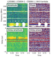 |
Fig. A.1. An example of a baseline affected by RFI in the 147–149 MHz range. The solid red line represent the baseline horizon line. |
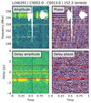 |
Fig. A.2. An example of a baseline affected by RFI in the 155–158 MHz range. The solid red line represent the baseline horizon line. |
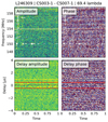 |
Fig. A.3. An example of a baseline broad-band RFI flagged by the delay-space baseline flagger. The solid red line represent the baseline horizon line. |
Appendix B: Cylindrically averaged power-spectra all nights
This appendix presents all cylindrically averaged power-spectra of the 14 processed nights before and after residual foregrounds removal (ML-GPR).
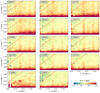 |
Fig. B.1. Cylindrically averaged power-spectra of all nights at z≈10.1, before ML-GPR. |
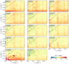 |
Fig. B.2. Cylindrically averaged power-spectra of all nights at z≈10.1, after ML-GPR. |
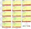 |
Fig. B.3. Cylindrically averaged power-spectra of all nights at z≈9.1, before ML-GPR. |
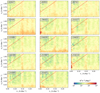 |
Fig. B.4. Cylindrically averaged power-spectra of all nights at z≈9.1, after ML-GPR. |
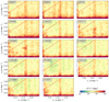 |
Fig. B.5. Cylindrically averaged power-spectra of all nights at z≈8.3, before ML-GPR. |
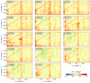 |
Fig. B.6. Cylindrically averaged power-spectra of all nights at z≈8.3, after ML-GPR. |
Appendix C: Posterior distribution of the GP model hyper-parameters
This appendix presents all posterior distribution of the GP model parameters for all three redshift bins, using a nested sampling algorithm.
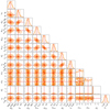 |
Fig. C.1. Posterior distribution of the GP model parameters derived using a nested sampling algorithm, at z≈10.1 |
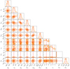 |
Fig. C.2. Posterior distribution of the GP model parameters derived using a nested sampling algorithm, at z≈9.1 |
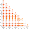 |
Fig. C.3. Posterior distribution of the GP model parameters derived using a nested sampling algorithm, at z≈8.3 |
All Tables
List of all observation nights analysed, with date, time, duration, and noise statistics.
GP model: summary of the model parameters, priors, and posteriors (median with 68% intervals).
upper limits at the 2-σ level () and the residual power after GPR minus the noise power () from the 10-night dataset, at given k bins for the three redshift ranges.
All Figures
|
Fig. 1. LOFAR-EoR HBA processing pipeline, describing the steps required to reduce the raw observed visibilities to the 21 cm signal power spectra. |
| In the text | |
|
Fig. 2. Normalised gain-spectra of the DI-calibration for frequency range 134–147 MHz, observation L254871. The one-step unregularised calibration (‘LOFAR 2020’, blue lines) is compared with the two-steps calibration (‘This work’, red lines). The delay corresponding to reflections in the 115-metre cables of LOFAR is denoted by a grey line, where a spectral feature is also observed, as expected. |
| In the text | |
|
Fig. 3. Signal-to-noise ratio (S/N) of the time-differenced solutions for all ∼28 000 sky components of LOFAR20 in real data. Clusters of components can be recognised since they share the same gain solutions. In total, there are 120 clusters in the image. The S/N is similar for most clusters, but showing a slight gradient to lower S/N values away from the phase centre. The components in the outer 14 clusters (with a flux weighted mean position more than 10 degrees away from the phase centre), indicated with red crosses, have been removed from the model used in the current analysis. |
| In the text | |
|
Fig. 4. Number of flagged baselines by some of the post-calibration visibility flagger, grouped by baseline length bins and categorised by different sources of contamination. Short baselines are predominantly affected, although certain frequency bands (147–149 MHz and 155–159 MHz) also show contamination on longer baselines |
| In the text | |
|
Fig. 5. Effect of post-calibration flagging steps on the 2D power spectra for observation L246309 in the frequency range 134–147 MHz. The left panel shows the power spectra before any calibration. The four middle panels display the ratio of power spectra before and after each successive flagging step, illustrating the progressive reduction of contamination. The four steps, shown in order, are: (1) post-calibration wide-bandwidth AOFlagger; (2) baseline flagging of delay-spectrum outliers above the horizon limit; (3) post-gridding flagging based on outlier detection in channels and uv-cells; and (4) post-gridding flagging of uv-cells contaminated by A-team sidelobes. The right panel shows the power spectra after all steps have been applied. While some steps increase thermal noise (e.g. step 2, which removes entire baselines), they are effective in reducing RFI-related contamination. In all panels, the foreground horizon line is shown as a solid red line, while the dashed green and black lines indicate the delay ranges where most of the power from Cas A and Cygnus A is expected, respectively. |
| In the text | |
|
Fig. 6. Variance as function of frequency for the ten combined nights of the three redshift bins. The top line (blue) shows the Stokes-I power after sky-model subtraction (DD-calibration). The middle line (orange) shows the variance of the residual after ML-GPR, the bottom line (dark grey) show the thermal noise level estimated from the gridded time-differenced visibilities. Flagged channels are shown in light grey. |
| In the text | |
|
Fig. 7. Noise standard deviation, in SEFD units, estimated from the channel-differenced noise at each uv-cell, after sky-model subtraction. Data are shown for the Stokes-I 10 nights combined z≈9.1 data cube. The trace of the Cas A and Cygnus A sources in the uv plane, which are fully flagged, are denoted with a blue and orange line, respectively. |
| In the text | |
|
Fig. 8. Coherence scales of the mode-mixing foreground GPR components for the three different redshift bins. The baseline dependence of the coherence scale is defined by Equation (10). Based on the estimated values of the θ parameters for the mode-mixing components, the coherence scales range approximately between 8 MHz and ≈2.5 MHz for redshift bins 8.3 (green line) and 9.1 (orange line). For redshift bin 10.1 (blue line), two mode-mixing components are required, yielding coherence scales ranging approximately between 10 MHz and 4 MHz for the first component (solid line), and between 3 MHz and 1 MHz for the second (dashed line). |
| In the text | |
|
Fig. 9. ML-GPR components decomposition of the residual Stokes-I for the three redshift bins. The residual Stokes-I data (blue line) are decomposed into the following components: foreground sky (red), mode-mixing (orange), excess (yellow), noise (green), and the 21 cm signal (magenta). The residual (grey line) represents the Stokes-I data after subtracting all the foreground components. The shaded area represents the 2-σ uncertainty. The top panel displays the cylindrically averaged power spectra as a function of k∥ (averaged over k⊥), while the bottom panels shows the spherically averaged power spectra. |
| In the text | |
|
Fig. 10. Cylindrically averaged power spectra of the ML-GPR component decomposition of the residual Stokes-I data for the three redshift bins. The top row shows the power spectra before ML-GPR. The second row shows the power spectra of the foreground components only (comprising the ‘sky’ and ‘mode-mixing’ components). The third row presents the power spectra of the residual data after subtracting the foregrounds using ML-GPR. The last row shows the ratio of the residual power to the thermal noise power. In all panels, the foreground horizon line is depicted by a dashed red line. The solid black line in the second row delimits the regions below which the foregrounds power is higher than the thermal noise power. |
| In the text | |
|
Fig. 11. Comparison between the current results and those of LOFAR20 at redshift z≈9.1. The top row shows the residual cylindrically averaged power spectra after GPR for the LOFAR20 dataset (left panel), the current dataset (middle panel), and the ratio between the two (right panel). The bottom row presents the ratio of the residual power to the thermal noise for the LOFAR20 dataset (left panel) and the current dataset (middle panel), accompanied by smoothed contour maps to emphasise the differences. In all panels, the foreground horizon line is indicated by a dashed red line. The significant reduction in residual power across the full k-space demonstrates the effectiveness of our improved data processing techniques. |
| In the text | |
|
Fig. 12. Final spherically averaged power spectra from the combined 10-night dataset, after ML-GPR residual foreground removal and noise bias removal, are shown as the blue line, with the shaded blue area representing the 95% confidence interval. Previous LOFAR upper limits from LOFAR20 (dark orange line) and Patil et al. (2017) (light orange line) are included for comparison. The theoretical thermal noise power spectrum is depicted by the dashed black line, and its 2-σ error is indicated by the dotted line. The new upper limits at z≈9.1 represent an improvement by a factor of 2–4 compared to the LOFAR 2020 results, achieved with comparable observational data. The shaded lavender-grey area represents the 2-σ upper limits that would be obtained if both the ‘excess’ and ‘foreground’ components were subtracted from the data. |
| In the text | |
|
Fig. 13. Recovery test of injected 21 cm signal, validating the post-processing flagging step. Top: effect after applying AOFlagger. Bottom: effect of the visibility flagging step. The difference between injected and recovered signal is within the 1 sigma uncertainty. |
| In the text | |
|
Fig. 14. Results of the injection test, validating the ML-GPR residual foreground removal step, with the Grizzly simulations. The top plots show the z-score as a function of k-mode. A total of 25 synthetic 21 cm signals are tested, each with four different intensities. Each box-plot represents the distribution of z-scores for all 25 cases, with different box-plot colours indicating different signal intensities. The central line represents the median z-score, the box edges indicate the 25th and 75th percentiles (interquartile range), the whiskers extend to the data points within 1.5 times the interquartile range, and individual points beyond the whiskers represent outliers. A negative z-score suggests absorption of the signal, with values below −2 indicating absorption beyond the 2-σ upper limits. The bottom panel shows the spherically averaged power spectrum (for |
| In the text | |
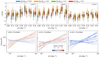 |
Fig. 15. Same as Figure 14 with the 21cmFAST simulations. |
| In the text | |
|
Fig. 16. Night-to-night cross-coherence for different regions of the cylindrically averaged power spectra, evaluated over all pairs of nights and across the three redshift bins. The top panels display density plots of the cross-coherence values, with colours indicating different regions of the power spectra (the specific regions are illustrated in the insets). The bottom panels present the individual cross-coherence values as a function of Local Sidereal Times (LST) time difference, along with a fitted trend line to highlight the overall pattern. For the redshift bin at z≈9.1 (middle panel), we also include in a dashed line the cross-coherence results from LOFAR20 for comparison. |
| In the text | |
|
Fig. A.1. An example of a baseline affected by RFI in the 147–149 MHz range. The solid red line represent the baseline horizon line. |
| In the text | |
|
Fig. A.2. An example of a baseline affected by RFI in the 155–158 MHz range. The solid red line represent the baseline horizon line. |
| In the text | |
|
Fig. A.3. An example of a baseline broad-band RFI flagged by the delay-space baseline flagger. The solid red line represent the baseline horizon line. |
| In the text | |
|
Fig. B.1. Cylindrically averaged power-spectra of all nights at z≈10.1, before ML-GPR. |
| In the text | |
|
Fig. B.2. Cylindrically averaged power-spectra of all nights at z≈10.1, after ML-GPR. |
| In the text | |
|
Fig. B.3. Cylindrically averaged power-spectra of all nights at z≈9.1, before ML-GPR. |
| In the text | |
|
Fig. B.4. Cylindrically averaged power-spectra of all nights at z≈9.1, after ML-GPR. |
| In the text | |
|
Fig. B.5. Cylindrically averaged power-spectra of all nights at z≈8.3, before ML-GPR. |
| In the text | |
|
Fig. B.6. Cylindrically averaged power-spectra of all nights at z≈8.3, after ML-GPR. |
| In the text | |
|
Fig. C.1. Posterior distribution of the GP model parameters derived using a nested sampling algorithm, at z≈10.1 |
| In the text | |
|
Fig. C.2. Posterior distribution of the GP model parameters derived using a nested sampling algorithm, at z≈9.1 |
| In the text | |
|
Fig. C.3. Posterior distribution of the GP model parameters derived using a nested sampling algorithm, at z≈8.3 |
| In the text | |
Current usage metrics show cumulative count of Article Views (full-text article views including HTML views, PDF and ePub downloads, according to the available data) and Abstracts Views on Vision4Press platform.
Data correspond to usage on the plateform after 2015. The current usage metrics is available 48-96 hours after online publication and is updated daily on week days.
Initial download of the metrics may take a while.