| Issue |
A&A
Volume 669, January 2023
|
|
|---|---|---|
| Article Number | A6 | |
| Number of page(s) | 5 | |
| Section | Cosmology (including clusters of galaxies) | |
| DOI | https://doi.org/10.1051/0004-6361/202244986 | |
| Published online | 20 December 2022 | |
Suppressing variance in 21 cm signal simulations during reionization
1
Institute for Computational Science, University of Zurich, Winterthurerstrasse 190, 8057 Zurich, Switzerland
e-mail: This email address is being protected from spambots. You need JavaScript enabled to view it.
2
Donostia International Physics Center (DIPC), Paseo Manuel de Lardizabal, 4, 20018 Donostia-San Sebastiàn, Spain
3
IKERBASQUE, Basque Foundation for Science, 48013 Bilbao, Spain
Received:
16
September
2022
Accepted:
25
October
2022
Abstract
Current best limits on the 21 cm signal during reionization are provided at large scales (≳100 Mpc). To model these scales, enormous simulation volumes are required, which are computationally expensive. We find that the primary source of uncertainty at these large scales is sample variance, which determines the minimum size of simulations required to analyse current and upcoming observations. In large-scale structure simulations, the method of ‘fixing’ the initial conditions (ICs) to exactly follow the initial power spectrum and ‘pairing’ two simulations with exactly out-of-phase ICs has been shown to significantly reduce sample variance. Here we apply this ‘fixing and pairing’ (F&P) approach to reionization simulations whose clustering signal originates from both density fluctuations and reionization bubbles. Using a semi-numerical code, we show that with the traditional method, simulation boxes of L ≃ 500 (300) Mpc are required to model the large-scale clustering signal at k = 0.1 Mpc−1 with a precision of 5 (10)%. Using F&P, the simulation boxes can be reduced by a factor of 2 to obtain the same precision level. We conclude that the computing costs can be reduced by at least a factor of 4 when using the F&P approach.
Key words: dark ages / reionization / first stars / cosmology: theory / Galaxy: formation / intergalactic medium
© The Authors 2022
 Open Access article, published by EDP Sciences, under the terms of the Creative Commons Attribution License (https://creativecommons.org/licenses/by/4.0), which permits unrestricted use, distribution, and reproduction in any medium, provided the original work is properly cited.
This article is published in open access under the Subscribe-to-Open model. This email address is being protected from spambots. You need JavaScript enabled to view it. to support open access publication.
1. Introduction
The 21 cm signal produced by the spin-flip transition of the ground state of neutral hydrogen present during the epoch of reionization (EoR) will be a treasure trove of information. It will teach us not only about the nature of the first luminous sources but also about the thermal and ionization history of the high-redshift (z ≳ 6) intergalactic medium (see Pritchard & Loeb 2012 for a review). Furthermore, it may help reveal the mysteries of the dark matter sector (e.g., Muñoz & Loeb 2018; Schneider 2018; Lopez-Honorez et al. 2019; Giri & Schneider 2022), find primordial black holes (Tashiro & Sugiyama 2013; Mena et al. 2019), and shed light on the origin of density fluctuations (Furugori et al. 2020; Cole & Silk 2021).
The 21 cm signal can be distinguished from the Rayleigh-Jeans tail of the cosmic microwave background radiation using radio telescopes. These telescopes will record a quantity known as the differential brightness temperature, which is given by
 (1)
(1)
where xHI and δ are the fraction of neutral hydrogen and the density fluctuation, respectively. The spin temperature, Ts, is the excitation temperature of the two spin states of the neutral hydrogen. The Tγ is the cosmic microwave background temperature at redshift z. In this work we assume the spin temperature to be saturated (Ts ≫ Tγ), which is a good approximation during the EoR. For simplicity, we furthermore ignore the redshift-space distortions (RSDs) of the signal.
The 21 cm signal from the EoR has not been detected yet. Current radio experiments, such as the LOw Frequency ARray (LOFAR; Mertens et al. 2020), Murchison Widefield Array (MWA; Trott et al. 2020), and Hydrogen Epoch of Reionization Array (HERA; The HERA Collaboration 2022) provide upper limits of the 21 cm power spectrum, which have helped rule out some extreme astrophysical models at z = 6 − 9 (e.g., Ghara et al. 2020, 2021). The thermal noise in the 21 cm signal observation increases with wave mode (e.g., Koopmans et al. 2015). Therefore, the best upper limits are currently obtained at wave modes k ∼ 0.1 Mpc−1. At even larger scales, the signal cannot be retrieved due to the presence of foreground contamination. Future observations by, for example, HERA and the Square Kilometre Array (SKA; Koopmans et al. 2015) are expected to detect the signal at k ∼ 0.1 − 1 Mpc−1 during their initial observation phases (e.g., Greig & Mesinger 2015).
The observed fields of view of radio telescopes are large enough for the observations at k ≳ 0.1 Mpc−1 to be less affected by cosmic variance. For example, the LOFAR upper limits were derived from observations with fields of view of 4° ×4°, which corresponds to k ∼ 0.01 Mpc−1 (Mertens et al. 2020). The error at the scales that we are interested in is dominated by the by various steps in the data processing pipeline, such as calibration and foreground mitigation (e.g., Mertens et al. 2020). However, the interpretation of these observations will be affected by the variance in simulations that use a box length (L) that is too close to the largest observed scales.
Iliev et al. (2014) find that simulations with L ≳ 150 Mpc are required to accurately model the distribution and growth of reionization bubbles. However, simulations of this size are known to be strongly affected by sample variance. At the relevant scales (k ∼ 0.1 Mpc−1), the limited number of wave modes (Nmodes) present in a simulation box of L ∼ 150 Mpc results in a sample error that resembles Poisson noise proportional to  . A similar study was done by Kaur et al. (2020), who included the pre-reionization era. To reduce sample variance at scales around k ∼ 0.1 Mpc−1, huge simulations (L ≳ 500 Mpc) are required (Ghara et al. 2020). Alternatively, one can model this signal by averaging over multiple realizations of smaller volume simulations (Mondal et al. 2020). Both approaches are very expensive, especially when considering that the reionization process may be driven by sources residing in dark matter mini-haloes (with masses of ≲108 M⊙), which need to be properly resolved (e.g., Giri & Schneider 2022).
In this work we explore a method known as ‘fixing and pairing’ (F&P), which has been shown to substantially reduce the variance in simulations of matter fluctuations at low redshifts (Pontzen et al. 2016; Angulo & Pontzen 2016). This method has been extensively used for high-precision predictions of the matter power spectrum (e.g., Villaescusa-Navarro et al. 2020; Angulo et al. 2021; Knabenhans et al. 2021) as well as biased tracers of the matter distribution (e.g., Villaescusa-Navarro et al. 2018; Maion et al. 2022). Here we apply the F&P approach for the first time to simulations of the 21 cm signal during reionization. In the next section we describe the simulations used in this study. In Sect. 3 we present our findings and conclude in Sect. 4.
2. Simulations
For this work we used the publicly available reionization simulation code 21cmFAST (Mesinger et al. 2011). We modified the initial condition (IC) generator of the code, adding the option of fixing the IC. The original (or Gaussian) method of 21cmFAST is summarized in Sect. 2.1, and our modifications are discussed in Sect. 2.2.
2.1. Gaussian method
21cmFAST initializes a Gaussian random field at the initial redshift (zinit = 50) using a linear power spectrum P(k, zinit) obtained from the Eisenstein & Hu (1999) fitting function. The ICs of the density perturbations are given by
![Mathematical equation: $$ \begin{aligned} \delta (\boldsymbol{k},z_\mathrm{init} ) = \sqrt{0.5P(k,z_\mathrm{init} )}\ [a_{\boldsymbol{k}}+ib_{\boldsymbol{k}}] , \end{aligned} $$](/articles/aa/full_html/2023/01/aa44986-22/aa44986-22-eq3.gif) (2)
(2)
where ak and bk are drawn from a Gaussian distribution 𝒩(0, 1) (Mesinger & Furlanetto 2007). The subsequent formation and evolution of structures are simulated using second-order Lagrangian perturbation theory (e.g., Bernardeau et al. 2002). The growth of ionized bubbles during reionization is modelled based on the formalism in Furlanetto et al. (2004).
In this work we assume the default values provided in Greig & Mesinger (2015) for the source parametrization (model 1). The virial temperature of the smallest haloes containing stars was set to Tvir ≃ 104.7 K. For simplicity, the ionizing efficiency of sources was set to ζ = 20. It should be noted that in reality ζ is expected to scale with source properties, for example with the mass of the hosting halo (see e.g., Park et al. 2019; Schneider et al. 2021). Finally, the maximum distance that photons can travel was set to Rmax = 15 Mpc, which models the unresolved absorbers. This is discussed further in Georgiev et al. (2022).
Regarding fiducial model 1, we investigated two more models where reionization is caused by rare and very efficient sources (model 2) and by a larger number of inefficient sources (model 3). The parameters of models 2 and 3 are given by {Tvir, ζ}={105.5 K, 200} and {Tvir, ζ}={104.3 K, 15}, respectively. We note that the parameters of all three models were chosen such that the reionization history remains unchanged. To study the influence of sample variance, we ran simulations with five different box lengths of L = 100, 150, 200, 300, and 400 Mpc, fixing the spatial resolution to 2 Mpc.
2.2. Fixing and pairing method
The F&P method for simulations is a two-step process that was introduced in Angulo & Pontzen (2016). The first step consists of ‘fixing’ the ICs and is achieved by replacing Eq. (2) with the following,
 (3)
(3)
Here we randomly drew θk from a flat distribution between 0 and 2π. This way the IC is ‘fixed’ to exactly give the linear power spectrum. The second step of the F&P method consists of running two ‘paired’ simulations (A and B) that are identical except that the phases of B are shifted by π with respect to those of A. This means that their density fields are inverted, that is, δA(k, zinit) = − δB(k, zinit). Fixing the ICs and taking the average over the summary statistics of two paired simulations, such as power spectra and bispectra, significantly reduces the sample variance.
In the first two panels of Fig. 1, we show slices of the 21 cm signal from two paired simulations produced with the F&P method. The slices are shown at z = 9, which corresponds to an early phase of reionization when the majority of the simulation volumes are still neutral (mean neutral fraction of xHI = 0.8). The bubbles are visible, and their positions are strongly correlated with the matter perturbations of the corresponding simulation. As the initial density fields between the two simulations are perfectly anti-correlated, the bubbles are anti-correlated as well. The two slices confirm that ionized regions in one simulation are still neutral in the other. We note, however, that this anti-correlation, while very strong during the early phases of reionization, reduces with time as the bubbles grow larger and merge.
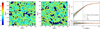 |
Fig. 1. Example of a pair of fixed simulations. First and second panel: slices of fixed and paired reionization simulations (A and B) at z = 9 (with a mean neutral fraction of xHI = 0.8). The colour map shows the differential brightness temperature between 0 and 50 mK. Third panel: 21 cm power spectra of the same paired simulations (blue and orange) along with those of 100 independent traditional simulations (grey lines). The mean power spectra of the traditional simulations and the two F&P simulations are shown as solid green and dotted red lines, respectively. For reference, the expected largest scale probed by SKA, k = 0.1 Mpc−1, is marked with a vertical line. |
The third panel of Fig. 1 shows the corresponding power spectra from the paired simulations (A and B). Also shown are the resulting F&P power spectrum, corresponding to the mean of the two, and, for comparison, the mean power spectrum of 100 independent realizations with the Gaussian method. The individual power spectra from each of these simulations are shown as well. The fact that the F&P result is nearly indistinguishable from this mean power spectrum is very promising. It qualitatively confirms that the F&P method can reduce the sample variance for simulations of the EoR. In the following section we investigate this result in a more quantitative manner.
3. Results
In this section we first show that sample variance is indeed the dominating modelling error for reionization simulations. We then investigate how we can reduce the sample variance using the F&P method and provide estimates for the smallest volumes that can be run without being dominated by sample variance.
3.1. Power spectrum
The power spectrum is expected to be the first detectable statistics of the 21 cm signal from radio interferometric experiments. We therefore require accurate predictions of the power spectrum with an associated theoretical error that ideally stays below the observational errors for all wave modes and redshifts. In terms of simulations, this means that we have to quantify errors related to, for example, the resolution, box size, and sample variance, selecting a simulation setup where such errors are sub-dominant. In this work we aim to quantify the minimum box size required for reionization simulations. This means we do not investigate resolution effects but focus on errors caused by missing large-scale modes and sample variance.
In Fig. 2 we show the ratio of the power spectra of smaller volumes compared to our largest simulation (L = 400 Mpc). Since these simulations are set up with the same realization of the density field, any deviations of smaller simulations are caused by missing modes that are larger than the box size. At k ≳ 0.1 Mpc−1, we find that the power spectra from small volume simulations (L = 150, 200, and 300 Mpc) deviate at a per cent level from the power spectrum measured in the L = 400 Mpc box. This is true for all the redshifts investigated. We also plot the case with L = 100 Mpc. This case shows large deviations at most wave modes as this volume is affected by the missing large-scale modes, which is consistent with the results from Iliev et al. (2014). Since the upcoming observations from the SKA are expected to provide measurements at k ≳ 0.1 Mpc−1 (e.g., Greig & Mesinger 2015), we conclude from Fig. 2 that a box size of L = 150 Mpc is sufficient to model the largest required modes at the 1% level. A similar study is presented in Greig et al. (2022).
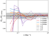 |
Fig. 2. Ratio of the power spectra produced with small simulation volumes (L = 100, 150, 200, and 300 Mpc) to that with the largest simulated volume (L = 400 Mpc). We mark k = 0.1 Mpc−1 with a vertical line, and the 1% level is the grey shaded region. The differences at k ≳ 0.1 Mpc−1 are within the 1% level for simulations with L ≳ 150 Mpc. |
We now turn our attention to the error caused by sample variance. The top panels of Fig. 3 show the standard deviations (σ) with respect to the mean power spectrum (μ) from 100 simulations at three different redshifts (corresponding to xHI = 0.8, 0.6, and 0.4 from left to right). The sample variances obtained with the Gaussian method (Sect. 2.1) are shown with different simulation volumes (L = 150, 200, 300, and 400 Mpc). The results from fixed simulations and F&P simulations are also shown. While fixing the ICs helps reduce the sample variance, a more significant improvement is obtained with the F&P method. Independent of the simulation volume and the k mode, F&P leads to a suppression of the cosmic variance by about a factor of ≳2 compared to the Gaussian method.
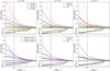 |
Fig. 3. Ratio of standard deviation on the power spectra to the mean power spectra estimated from 100 simulations at early (left panels), middle (middle panels), and late (right panels) stages of reionization. We also mark the wave mode k = 0.1 Mpc−1 with vertical lines. The top panels show the results from four different simulation volumes (150 Mpc: red, 200 Mpc: blue, 300 Mpc: orange, 400 Mpc: green) for the Gaussian (dotted), fixed IC (dashed), and F&P (solid) methods. We see that the fixed IC and F&P methods reduce the error on the power spectra by about 1.5 and 2 times, respectively, compared to the Gaussian method. The bottom panels show the results for three different reionization models (1: blue, 2: violet, 3: brown). Both the fixed IC and F&P methods work in a similar manner for all the models. We have also included, in the bottom sub-panels, the ratio of standard deviation to that of the Gaussian method. |
In the bottom panels of Fig. 3, we focus on the L = 200 Mpc box, providing results from astrophysical models 1, 2, and 3. All three models provide a similar improvement, confirming that our results are only weakly dependent on the choice of astrophysical model.
Comparing the different simulation volumes shown in Fig. 3, we conclude that the F&P method can obtain the same sample variance for simulations that have a two times smaller box size than with the traditional approach. For example, at k = 0.1 Mpc−1, the F&P approach gives a similar sample variance for the L = 200 Mpc simulations compared to the L = 400 Mpc simulations with the Gaussian method at all redshifts. Reducing the box size by a factor of 2 improves the speed and reduces the memory requirement by at least a factor of 8. Since two simulations are required for the F&P approach, a gain of at least a factor of four is expected.
3.2. Bispectrum
The 21 cm signal is expected to be highly non-Gaussian. As a consequence, higher-order statistics will have to be used to obtain all the available information contained in the 21 cm density field. Measuring the bispectrum, ℬ, consists of an obvious step in that direction (e.g., Majumdar et al. 2018), which is given by
 (4)
(4)
where δD is the Dirac delta function, and B(k1, k2, k3) depends on the configuration of triangles formed by the three wave vectors (k1, k2, and k3). Here we study two configurations, an equilateral triangle (k1 = k2 = k3) and a scalene triangle (k1 = k2/2 = 0.1 Mpc−1). We used the publicly available package BIFFT (Watkinson et al. 2021) to measure the bispectra of our simulations.
The top panel of Fig. 4 shows the equilateral ℬ at z = 9 (xHI = 0.8) for the simulations shown in Fig. 1. The 100 simulations with the Gaussian method are plotted with their mean, and simulations A and B are highlighted. Just as for the power spectrum, we observe significant sample variance in the equilateral ℬ at small wave modes (k ≲ 0.2 Mpc−1). For reference, we again mark k = 0.1 Mpc−1. Finally, the equilateral ℬ of the F&P simulations is also shown. It lies very close to the mean value of the 100 independent simulations, confirming the results obtained with the power spectrum. As a consequence, we expect the F&P method to yield a similar improvement regarding the sample variance of the equilateral ℬ.
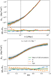 |
Fig. 4. 21 cm bispectra from 100 simulations at z = 9 produced in L = 300 Mpc simulation volumes plotted with grey lines, with the mean shown with green lines. Top panel: equilateral bispectra as a function of wave modes. We also mark k = 0.1 Mpc−1 with a vertical line and observe that the variance increases below this scale. Bottom panel: scalene bispectrum as a function of the angle between the two wave vectors, k1 and k2. The 21 cm bispectra corresponding to simulations A and B, shown in Fig. 1, are given with blue and orange lines, respectively. With these two simulations, we can estimate the bispectrum (red lines) that is very close to the mean bispectrum in both panels. |
Very similar conclusions can be drawn when investigating the scalene ℬ shown in the bottom panel of Fig. 4. Here the ℬ is given as a function of the opening angle between the two wave vectors, k1 and k2 (θ = cos−1(k1.k2/(k1k2)). As k1 = k2/2 = 0.1 Mpc−1, this ℬ probes the non-Gaussianity at large scales for all values of θ. Therefore, we observe a large variance for all values of the angle θ. We again find that the F&P simulations help in getting close to the mean ℬ estimated from 100 traditional simulations. In this section we have argued that the sample variance of the ℬ can be suppressed by the F&P method in a similar way as for the power spectrum. We limited ourselves to a qualitative analysis of two particular ℬ configurations for a single redshift. We note, however, that the non-Gaussian information contained in the 21 cm bispectra is very rich, showing a complicated evolution during the EoR (Majumdar et al. 2018). A more thorough investigation of the effect of sample variance on higher-order statistics is left for future work.
4. Conclusions
Numerical simulations of the EoR are very expensive as they need to simultaneously resolve small sources and cover large cosmological volumes. In this work we used the semi-numerical code 21cmFAST to investigate the minimum box size (L) a simulation needs to produce unbiased results. We thereby primarily focused on the 21 cm power spectrum at scales corresponding to k = 0.1 − 1 Mpc−1, where future observations from, for example, HERA and SKA are expected to detect the 21 cm signal.
First, we performed a comparison of power spectra from simulations with the same initial density field but different box lengths (L = 100, 150, 200, 300, and 400 Mpc). The analysis revealed that power spectra from L ≳ 150 Mpc agree within a per cent in the regime of k = 0.1 − 1 Mpc−1. We conclude that a box size of L = 150 Mpc is sufficient to be unbiased by missing large-scale modes
We then studied the sample variance (sometimes referred to as cosmic variance), which is known to affect the large-scale power spectrum at a more significant level. Using the Gaussian method, we show that simulation volumes with a box length of at least L = 400 Mpc are required to reduce the uncertainty to less than 10% at k = 0.1 Mpc−1. The sample variance can be reduced by about a factor of 1.5 by fixing the ICs. With this method, we can achieve an error of ≲10% at k ≈ 0.1 Mpc−1 by using a smaller simulation box of L = 300 Mpc instead. We note that the reionization simulations of the THESAN project (Kannan et al. 2022) were fixed, but they did not study the impact of pairing.
As a further step, we applied the F&P method to reionization simulations. The method consists of taking the average power spectrum from two fixed simulations with inverted ICs. While F&P simulations have been successfully used to suppress sample variance for low-redshift cosmological simulations, they have never been used in the context of reionization. We show that the F&P method can further reduce the effect of sample variance to below 10% for a box size of L = 200 Mpc. We also tested the robustness of our results by changing the astrophysical parameters assuming a model with fewer, more efficient sources and a model with a larger number of inefficient sources. We find similar improvements using these models, which means that our general conclusions remain independent of the assumed astrophysical model.
Finally, we investigated the effect of sample variance on the 21 cm bispectrum. We find that sample variance affects the bispectrum and the power spectrum similarly. The F&P method is expected to improve the theoretical predictions for higher-order statistics as well, in agreement with findings from cosmological simulations at low redshifts (Angulo & Pontzen 2016).
We note that we have not included RSD in our simulation. We do not expect a significant impact on our findings since, to the first order, the RSD just boosts the signal at all wave modes (e.g., Ross et al. 2021), which will cancel out in the relative error studied here. In the future, we will explore this effect in detail.
In general, we conclude that the F&P method allows the sample variance caused by the finite simulation volume to be significantly reduced. For reionization, this means that two F&P simulations with L = 200 Mpc are sufficient to predict the 21 cm signal in the regime of k = 0.1 − 1 Mpc−1 to better than 10%. This give us of a speed up of a factor of ≳4 compared to previous simulation methods.
Acknowledgments
We thank Bradley Greig for useful comments. This research was supported by the Munich Institute for Astro-, Particle and BioPhysics (MIAPbP) which is funded by the Deutsche Forschungsgemeinschaft (DFG, German Research Foundation) under Germany’s Excellence Strategy – EXC-2094 – 390783311. SKG and AS are supported by the Swiss National Science Foundation via the Grant No. PCEFP2_181157. FM and REA acknowledge the support of the ERC-StG number 716151 (BACCO). The simulations were analysed using TOOLS21CM (Giri et al. 2020).
References
- Angulo, R. E., & Pontzen, A. 2016, MNRAS, 462, L1 [NASA ADS] [CrossRef] [Google Scholar]
- Angulo, R. E., Zennaro, M., Contreras, S., et al. 2021, MNRAS, 507, 5869 [NASA ADS] [CrossRef] [Google Scholar]
- Bernardeau, F., Colombi, S., Gaztanaga, E., & Scoccimarro, R. 2002, Phys. Rep., 367, 1 [NASA ADS] [CrossRef] [Google Scholar]
- Cole, P. S., & Silk, J. 2021, MNRAS, 501, 2627 [NASA ADS] [CrossRef] [Google Scholar]
- Eisenstein, D. J., & Hu, W. 1999, ApJ, 511, 5 [Google Scholar]
- Furlanetto, S. R., Zaldarriaga, M., & Hernquist, L. 2004, ApJ, 613, 1 [NASA ADS] [CrossRef] [Google Scholar]
- Furugori, K., Abe, K. T., Tanaka, T., et al. 2020, MNRAS, 494, 4334 [NASA ADS] [CrossRef] [Google Scholar]
- Georgiev, I., Mellema, G., Giri, S. K., & Mondal, R. 2022, MNRAS, 513, 5109 [NASA ADS] [CrossRef] [Google Scholar]
- Ghara, R., Giri, S. K., Mellema, G., et al. 2020, MNRAS, 493, 4728 [NASA ADS] [CrossRef] [Google Scholar]
- Ghara, R., Giri, S. K., Ciardi, B., Mellema, G., & Zaroubi, S. 2021, MNRAS, 503, 4551 [NASA ADS] [CrossRef] [Google Scholar]
- Giri, S. K., & Schneider, A. 2022, Phys. Rev. D, 105, 083011 [NASA ADS] [CrossRef] [Google Scholar]
- Giri, S., Mellema, G., & Jensen, H. 2020, J. Open Source Softw., 5, 2363 [NASA ADS] [CrossRef] [Google Scholar]
- Greig, B., & Mesinger, A. 2015, MNRAS, 449, 4246 [NASA ADS] [CrossRef] [Google Scholar]
- Greig, B., Wyithe, J. S. B., Murray, S. G., Mutch, S. J., & Trott, C. M. 2022, MNRAS, 516, 5588 [NASA ADS] [CrossRef] [Google Scholar]
- Iliev, I. T., Mellema, G., Ahn, K., et al. 2014, MNRAS, 439, 725 [Google Scholar]
- Kannan, R., Garaldi, E., Smith, A., et al. 2022, MNRAS, 511, 4005 [NASA ADS] [CrossRef] [Google Scholar]
- Kaur, H. D., Gillet, N., & Mesinger, A. 2020, MNRAS, 495, 2354 [NASA ADS] [CrossRef] [Google Scholar]
- Knabenhans, M., Stadel, J., Potter, D., et al. 2021, MNRAS, 505, 2840 [NASA ADS] [CrossRef] [Google Scholar]
- Koopmans, L., Pritchard, J., Mellema, G., et al. 2015, in AASKA14, 1 [Google Scholar]
- Lopez-Honorez, L., Mena, O., & Villanueva-Domingo, P. 2019, Phys. Rev. D, 99, 023522 [NASA ADS] [CrossRef] [Google Scholar]
- Maion, F., Angulo, R. E., Zennaro, M., et al. 2022, JCAP, 2022, 036 [CrossRef] [Google Scholar]
- Majumdar, S., Pritchard, J. R., Mondal, R., et al. 2018, MNRAS, 476, 4007 [NASA ADS] [CrossRef] [Google Scholar]
- Mena, O., Palomares-Ruiz, S., Villanueva-Domingo, P., & Witte, S. J. 2019, Phys. Rev. D, 100, 043540 [NASA ADS] [CrossRef] [Google Scholar]
- Mertens, F. G., Mevius, M., Koopmans, L. V., et al. 2020, MNRAS, 493, 1662 [NASA ADS] [CrossRef] [Google Scholar]
- Mesinger, A., & Furlanetto, S. 2007, ApJ, 669, 663 [Google Scholar]
- Mesinger, A., Furlanetto, S., & Cen, R. 2011, MNRAS, 411, 955 [Google Scholar]
- Mondal, R., Fialkov, A., Fling, C., et al. 2020, MNRAS, 498, 4178 [NASA ADS] [CrossRef] [Google Scholar]
- Muñoz, J. B., & Loeb, A. 2018, Nature, 557, 684 [Google Scholar]
- Park, J., Mesinger, A., Greig, B., & Gillet, N. 2019, MNRAS, 484, 933 [NASA ADS] [CrossRef] [Google Scholar]
- Pontzen, A., Slosar, A., Roth, N., & Peiris, H. V. 2016, Phys. Rev. D, 93, 103519 [NASA ADS] [CrossRef] [Google Scholar]
- Pritchard, J. R., & Loeb, A. 2012, Rep. Prog. Phys., 75, 086901 [NASA ADS] [CrossRef] [Google Scholar]
- Ross, H. E., Giri, S. K., Mellema, G., et al. 2021, MNRAS, 506, 3717 [NASA ADS] [CrossRef] [Google Scholar]
- Schneider, A. 2018, Phys. Rev. D, 98, 063021 [NASA ADS] [CrossRef] [Google Scholar]
- Schneider, A., Giri, S. K., & Mirocha, J. 2021, Phys. Rev. D, 103, 083025 [NASA ADS] [CrossRef] [Google Scholar]
- Tashiro, H., & Sugiyama, N. 2013, MNRAS, 435, 3001 [NASA ADS] [CrossRef] [Google Scholar]
- The HERA Collaboration (Abdurashidova, Z., et al.) 2022, ApJ, 925, 221 [NASA ADS] [CrossRef] [Google Scholar]
- Trott, C. M., Jordan, C., Midgley, S., et al. 2020, MNRAS, 493, 4711 [NASA ADS] [CrossRef] [Google Scholar]
- Villaescusa-Navarro, F., Naess, S., Genel, S., et al. 2018, ApJ, 867, 137 [NASA ADS] [CrossRef] [Google Scholar]
- Villaescusa-Navarro, F., Wandelt, B. D., Anglés-Alcázar, D., et al. 2020, ApJS, 250, 2 [CrossRef] [Google Scholar]
- Watkinson, C. A., Majumdar, S., Pritchard, J. R., & Mondal, R. 2021, Astrophysics Source Code Library [record ascl:2106.036] [Google Scholar]
All Figures
|
Fig. 1. Example of a pair of fixed simulations. First and second panel: slices of fixed and paired reionization simulations (A and B) at z = 9 (with a mean neutral fraction of xHI = 0.8). The colour map shows the differential brightness temperature between 0 and 50 mK. Third panel: 21 cm power spectra of the same paired simulations (blue and orange) along with those of 100 independent traditional simulations (grey lines). The mean power spectra of the traditional simulations and the two F&P simulations are shown as solid green and dotted red lines, respectively. For reference, the expected largest scale probed by SKA, k = 0.1 Mpc−1, is marked with a vertical line. |
| In the text | |
|
Fig. 2. Ratio of the power spectra produced with small simulation volumes (L = 100, 150, 200, and 300 Mpc) to that with the largest simulated volume (L = 400 Mpc). We mark k = 0.1 Mpc−1 with a vertical line, and the 1% level is the grey shaded region. The differences at k ≳ 0.1 Mpc−1 are within the 1% level for simulations with L ≳ 150 Mpc. |
| In the text | |
|
Fig. 3. Ratio of standard deviation on the power spectra to the mean power spectra estimated from 100 simulations at early (left panels), middle (middle panels), and late (right panels) stages of reionization. We also mark the wave mode k = 0.1 Mpc−1 with vertical lines. The top panels show the results from four different simulation volumes (150 Mpc: red, 200 Mpc: blue, 300 Mpc: orange, 400 Mpc: green) for the Gaussian (dotted), fixed IC (dashed), and F&P (solid) methods. We see that the fixed IC and F&P methods reduce the error on the power spectra by about 1.5 and 2 times, respectively, compared to the Gaussian method. The bottom panels show the results for three different reionization models (1: blue, 2: violet, 3: brown). Both the fixed IC and F&P methods work in a similar manner for all the models. We have also included, in the bottom sub-panels, the ratio of standard deviation to that of the Gaussian method. |
| In the text | |
|
Fig. 4. 21 cm bispectra from 100 simulations at z = 9 produced in L = 300 Mpc simulation volumes plotted with grey lines, with the mean shown with green lines. Top panel: equilateral bispectra as a function of wave modes. We also mark k = 0.1 Mpc−1 with a vertical line and observe that the variance increases below this scale. Bottom panel: scalene bispectrum as a function of the angle between the two wave vectors, k1 and k2. The 21 cm bispectra corresponding to simulations A and B, shown in Fig. 1, are given with blue and orange lines, respectively. With these two simulations, we can estimate the bispectrum (red lines) that is very close to the mean bispectrum in both panels. |
| In the text | |
Current usage metrics show cumulative count of Article Views (full-text article views including HTML views, PDF and ePub downloads, according to the available data) and Abstracts Views on Vision4Press platform.
Data correspond to usage on the plateform after 2015. The current usage metrics is available 48-96 hours after online publication and is updated daily on week days.
Initial download of the metrics may take a while.