| Issue |
A&A
Volume 699, July 2025
|
|
|---|---|---|
| Article Number | A206 | |
| Number of page(s) | 26 | |
| Section | Extragalactic astronomy | |
| DOI | https://doi.org/10.1051/0004-6361/202553977 | |
| Published online | 09 July 2025 | |
Modelling the selection of galaxy groups with end-to-end simulations
1
Department of Astronomy, University of Geneva, Ch. d’Ecogia 16, CH-1290 Versoix, Switzerland
2
Department of Physics, University of Helsinki, Gustaf Hällströmin katu 2, 00560 Helsinki, Finland
3
Max-Planck-Institut für extraterrestrische Physik (MPE), Giessenbachstraße 1, D-85748 Garching bei München, Germany
4
Department of Computer Science, Aalto University, PO Box 15400, Espoo, FI-00076, Finland
5
Tartu Observatory, University of Tartu, Observatooriumi 1, 61602 Tõravere, Estonia
6
Estonian Academy of Sciences, Kohtu 6, 10130 Tallinn, Estonia
7
Dr. Karl Remeis-Observatory and Erlangen Centre for Astroparticle Physics, Friedrich-Alexander Universität Erlangen-Nürnberg, Sternwartstr. 7, 96049 Bamberg, Germany
8
Institut d’Astrophysique de Paris (UMR 7095: CNRS & Sorbonne Université), 98 bis Bd Arago, F-75014 Paris, France
9
INAF/IASF-Milano, Via A. Corti 12, 20133 Milano, Italy
10
INAF, Osservatorio di Astrofisica e Scienza dello Spazio, via Piero Gobetti 93/3, 40129 Bologna, Italy
11
Center for Astrophysics | Harvard & Smithsonian, 60 Garden Street, Cambridge, MA 02138, USA
12
Centre for Radio Astronomy Techniques and Technologies, Department of Physics and Electronics, Rhodes University, PO Box 94, Makhanda 6140, South Africa
13
South African Radio Astronomy Observatory, Black River Park North, 2 Fir St, Cape Town 7925, South Africa
14
Centre for Astrophysics Research, Department of Physics, Astronomy and Mathematics, University of Hertfordshire, College Lane, Hatfield AL10 9AB, UK
15
Kavli Institute for Cosmology, University of Cambridge, Madingley Road, Cambridge, CB3 0HA, UK
16
Department of Physics and Astronomy, The University of Alabama in Huntsville, Huntsville, AL 35899, USA
17
Max-Planck-Institut für Astronomie, Königstuhl 17, 69117 Heidelberg, Germany
⋆ Corresponding author: This email address is being protected from spambots. You need JavaScript enabled to view it.
Received:
31
January
2025
Accepted:
3
June
2025
Abstract
Context. Feedback from supernovae and active galactic nuclei (AGN) shapes the galaxy formation and evolution, but its impact remains unclear. Galaxy groups offer a crucial probe to determine this impact because their gravitational binding energy is comparable to the energy that is available from their central AGN. The XMM-Newton Group AGN Project (X-GAP) is a sample of 49 groups that were selected in the X-ray (ROSAT) and optical (SDSS) bands and provides a benchmark for hydrodynamical simulations.
Aims. For this comparison, it is essential to understand the selection effects. We model the selection function of X-GAP by forward-modelling the detection process in the X-ray and optical bands.
Methods. Using the Uchuu N-body simulation, we built a dark matter halo light cone, predicted X-ray group properties with a neural network trained on hydrodynamical simulations, and assigned matching observed properties to the galaxies. We compared the selected sample to the parent population in the light cone.
Results. Our method provided a sample that matched the observed distribution of the X-ray luminosity and velocity dispersion. A completeness of 50% was reached at a velocity dispersion of 450 km/s in the X-GAP redshift range. The selection is driven by X-ray flux, with a secondary dependence on the velocity dispersion and redshift. We estimated a purity level of 93% for the X-GAP parent sample. We calibrated the relation of the velocity dispersion to the halo mass. We found a normalisation and slope that agree with the literature and an intrinsic scatter of about 0.06 dex. The measured velocity dispersion is only accurate within 10% for rich systems with more than about 20 members, and the velocity dispersion for groups with fewer than 10 members is biased at more than 20%.
Conclusions. The X-ray follow-up refines the optical selection and enhances the purity, but reduces completeness. In an SDSS-like set-up, measurement errors for the velocity dispersion dominate the intrinsic scatter. Our selection model enables unbiased comparisons of thermodynamic properties and gas fractions between X-GAP groups and hydrodynamical simulations.
Key words: methods: data analysis / surveys / galaxies: clusters: intracluster medium / galaxies: groups: general / large-scale structure of Universe / X-rays: galaxies: clusters
© The Authors 2025
 Open Access article, published by EDP Sciences, under the terms of the Creative Commons Attribution License (https://creativecommons.org/licenses/by/4.0), which permits unrestricted use, distribution, and reproduction in any medium, provided the original work is properly cited.
This article is published in open access under the Subscribe to Open model. This email address is being protected from spambots. You need JavaScript enabled to view it. to support open access publication.
1. Introduction
The large-scale structure (LSS) of the Universe evolves under the action of gravity following a bottom-up scenario (Navarro et al. 1996; Mo & White 2002; Springel et al. 2005; Fakhouri et al. 2010). The massive dark matter haloes we observe today in the nodes of the LSS are the end result of a process of merging and accretion from smaller haloes that formed in the early Universe from the collapse of initial perturbations in the density field. The behaviour of baryonic components such as gas and stars within the distribution of dark matter has been a key scientific puzzle for the past few decades. Feedback from active galactic nuclei (AGN, Padovani et al. 2017) has been suggested as a solution to a variety of questions, such as the suppression of cooling flows towards the centre of galaxy clusters (McNamara & Nulsen 2007; Gitti et al. 2012; Fabian 2012; Hlavacek-Larrondo et al. 2022; Bourne & Yang 2023), the quenching of star formation to reproduce the shape of the observed galaxy stellar mass function in simulations (Silk & Rees 1998; Pillepich et al. 2018), and the origin of scaling relations between galaxy properties and the mass of a supermassive black hole (SMBH) (Magorrian et al. 1998; Kauffmann & Haehnelt 2000; Kormendy & Ho 2013; Sahu et al. 2019).
Galaxy groups represent a key mass scale in this context because their gravitational binding energy is comparable to the output energy of the central AGN. Therefore, galaxy groups are very sensitive to the physics of AGN feedback. They are located at the peak of the mass density at the current epoch (Tinker et al. 2008). Groups of galaxies were historically first detected and studied in the optical and infrared bands, as collections of their member galaxies identified as over-densities in angular and redshift distributions (Abell 1958; Zwicky et al. 1963; Huchra & Geller 1982; Geller & Huchra 1983; Beers et al. 1990). Since then, various works presented similar methods for identifying groups from galaxy surveys, including phase-space methods (Mamon et al. 2013), the identification of red-sequence galaxies (Gladders & Yee 2000; Saro et al. 2013; Rykoff et al. 2014; Licitra et al. 2016), friends-of-friends (FoF) algorithms (Trevese et al. 2007; Muñoz-Cuartas & Müller 2012; Wen et al. 2012; Tempel et al. 2012), and modified FoF algorithms (Tempel et al. 2018; Lambert et al. 2020). Groups are often characterised in terms of the velocity dispersion of their galaxy members (Mamon et al. 2010; Gozaliasl et al. 2020); we refer to Old et al. (2014, 2015) for a comprehensive description and review about optical detection and mass estimate of galaxy groups). Galaxy groups are also often identified in X-rays through thermal bremsstrahlung and line emission from the hot gas that fills their potential wells (e.g. Böhringer et al. 2000; Rosati et al. 2002; Gozaliasl et al. 2014, 2019) and reaches temperatures between 106 and 108 K (Sanders 2023). Wide-field survey instruments in the X-ray band, such as ROSAT1 (Truemper 1982) and eROSITA2 (Merloni et al. 2012; Predehl et al. 2021), are therefore suitable to detect these objects. X-ray observations show prominent features such as cavities in the intra-group medium (IGrM) that are produced by massive AGN outflows (Bîrzan et al. 2008; Gastaldello et al. 2009; Randall et al. 2015). When the outburst is supersonic, shock waves propagating perpendicular to the outflow become visible (Liu et al. 2019).
The behaviour of the gaseous atmosphere is strongly connected with both gravitational and non-gravitational processes. The physical connection between these two types of properties is therefore related to the thermodynamic quantities describing the gas state. For example, AGN feedback tends to disrupt the gas in a more dramatic manner than massive clusters, causing an excess entropy in the core (Ponman et al. 1999) and/or in the outskirts, as observed by Finoguenov et al. (2002), Ponman et al. (2003). The combination of data from different wavelengths allowed us to consider these questions from various points of view. The Complete Local Volume Groups Sample (CLoGS, O’Sullivan et al. 2017) started from optical groups from the all-sky Lyon Galaxy Group catalogue (LGG, Garcia 1993) and combined them with X-ray observations from Chandra and XMM-Newton and with radio data from the Giant Metre wave Radio Telescope (GMRT) and the Very Large Array (VLA). Their sample was limited to the local Universe within 80 Mpc and focused on the properties of the brightest group galaxies (BGGs; O’Sullivan et al. 2018; Kolokythas et al. 2018, 2019). Later studies provided a more systematic analysis of thermodynamical properties for groups out to large radii, even up to R500c3, using both XMM-Newton (Johnson et al. 2009) and Chandra (Sun et al. 2009). More recently, Bahar et al. (2024) compared a large sample of 1178 groups that were detected in the first eROSITA all-sky survey to various hydrodynamical simulations. They found that the entropy profiles agree well between observations and simulations, whereas the groups core and inner part of the profile show some inconsistencies. This means that group properties might be a direct tracer of the AGN feedback mechanism.
Currently, hydrodynamical cosmological simulations include the implementation of AGN feedback in various forms and recipes. Some simulations, such as cosmo-OWLS (Le Brun et al. 2014), EAGLE (Schaye et al. 2015), and BAHAMAS (McCarthy et al. 2017), rely on an isotropic and thermal response to gas accretion onto the SMBH (see e.g. Booth & Schaye 2009). The gas surrounding the central black hole is heated when the AGN turns on, which suppresses gas cooling and hence star formation. Illustris (Vogelsberger et al. 2014) has a separate radio mode that injects off-set hot bubbles to mimic radio lobes. This concept was also used by the Fable Simulations (Henden et al. 2018). Other works, including HorizonAGN (Dubois et al. 2016), MAGNETICUM (Dolag et al. 2016), IllustrisTNG (Pillepich et al. 2018), SIMBA (Davé et al. 2019), and Flamingo (Schaye et al. 2023), added a kinetic feedback scheme, in which part of the energy injected by the AGN is converted into kinetic energy of the surrounding gas. This drives outflows out of the central SMBH and is more similar to a standard supernova feedback approach (Springel & Hernquist 2003).
Most simulations are tuned to reproduce a standard set of observables, which mainly are the galaxy stellar mass function, but also the gas fraction for clusters in the local Universe (BAHAMAS, Fable, and Flamingo). Although different simulations agree on the prediction of the quantities used to tune them, this is not necessarily the case for the inferred quantities. The predictions of the gas content and radial profiles of thermo-dynamical quantities, such as pressure and entropy, differ significantly between various works in the regime of galaxy groups, as highlighted by the reviews from Eckert et al. (2021), Oppenheimer et al. (2021), Gastaldello et al. (2021).
High-quality and multi-wavelength observations of galaxy groups are required to inform simulations in this regime. This is the primary goal of the XMM-Newton Group AGN Project (X-GAP, Eckert et al. 2024), which is a large program on XMM-Newton dedicated to 49 galaxy groups that aims to measure the impact of AGN feedback on the IGrM out to R500c. X-GAP is selected from the parent All-sky X-ray Extended Sources project (AXES, Damsted et al. 2024; Khalil et al. 2024), which combines the X-ray detection from the ROSAT all-sky survey using wavelet filters (Käfer et al. 2019) and optical FoF groups detected in the Sloan Digital Sky Survey (SDSS, Blanton et al. 2017) by Tempel et al. (2017). On the one hand, the optical detection of galaxy groups using galaxy members is affected by projection effects that typically arise in photometric data (see e.g. redmapper Rykoff et al. 2014). Spectroscopic information (Robotham et al. 2011; Tinker 2021) alleviates the projection effects, but a few issues still remain, such as low statistics, spectroscopic completeness, or redshift space distortions. On the other hand, the X-ray detection of groups is affected by a preferential selection for bright and peaked objects (this is the notion of cool core bias, Eckert et al. 2011), and only at relatively low redshift due to the shallow depth of X-ray surveys such as ROSAT (Ponman et al. 1999) and eROSITA (Bulbul et al. 2024; Bahar et al. 2024). The double selection in X-GAP is devised to obtain a complete and pure sample of galaxy groups that is to be compared to hydrodynamical simulations.
In this context, understanding the X-GAP completeness level is key to assessing whether any statement about AGN feedback resulting from its analysis is valid for a fair subsample of the overall group population in the Universe. This concept is encoded in the selection function, that is, the probability of a detection as a function of a given set of properties. In astronomical surveys, it is in fact often fruitful to model the incompleteness and exploit larger amounts of data than to restrict the study to a very complete sample with a high signal-to-noise ratio at the cost of losing many sources that lie closer to the detection limit (Rix et al. 2021; Clerc et al. 2024). The selection function is therefore a key component of the scaling relation and the cosmological analysis (see e.g, Pacaud et al. 2018; Bahar et al. 2022; Ghirardini et al. 2024; Artis et al. 2024) because it addresses the population of undetected objects in a statistical way.
We developed a framework for modelling the X-GAP selection function quantitatively by forward-modelling the selection process using end-to-end simulations. Similar approaches were recently dedicated to modelling the eROSITA X-ray selection function (Seppi et al. 2022; Clerc et al. 2024; Marini et al. 2024). A multi-wavelength approach to assess the sample properties with simulations is key to obtaining observational constraints that are representative of the underlying population (Marini et al. 2025; Popesso et al. 2024). We constructed a full-sky light cone starting from the Uchuu set of N-body simulations (Ishiyama et al. 2021). We used dedicated SDSS mocks based on Uchuu (Dong-Páez et al. 2024) to develop the optical side of our simulation. We populated our mock sky with X-rays using the AGN model from Comparat et al. (2019) and a new model for clusters and groups informed by hydrodynamical simulations. We forward-modelled the X-ray observations with the software called simulation of X-ray telescopes (SIXTE, Dauser et al. 2019). We reproduced the detection schemes in X-rays (Damsted et al. 2024) and optical bands (Tempel et al. 2017). We focused on selecting the parent sample because replicating the cuts in source size (angular size of R500c smaller than 15 arcmin to fit in the XMM-Newton field of view) and galaxy members (more than or equal to eight spectroscopic members) is then straightforward (Eckert et al. 2024). We evaluated and modelled the X-GAP selection function in terms of observables without directly modelling the mass selection. This makes the selection function more flexible against specific modelling choices, which may impact the relation between mass and luminosity. Finally, we calibrated the scaling relation between the line-of-sight velocity dispersion and the halo mass of the galaxy members.
This paper is organised as follows. In Section 2 we explain the strategy in our end-to-end simulation. In Section 3 we describe the neural network model we used to assign X-ray profiles and temperature to dark matter haloes. In Section 4 we elaborate on the treatment of each catalogue for input haloes, X-rays, and optical detections. In Section 5 we describe sample properties such as purity and completeness, and we model the selection function. In Section 6 we calibrate the scaling relation between the velocity dispersion and halo mass. Finally, in Section 7 we elaborate our findings in terms of the dynamical state of dark matter haloes and summarize our results in comparison to other works. When not otherwise specified, we assume the cosmological parameters from Planck Collaboration VI (2020), those used for simulating the Uchuu Universe, that is, ΩM = 0.3089, ΩB = 0.0486, σ8 = 0.8159, and H0 = 67.74 km/s/Mpc. We use X-ray luminosities within R500c in the 0.5–2.0 keV band.
2. Simulation strategy
Our strategy was to forward-model the galaxy group selection with end-to-end simulations, as shown in Fig. 1. We started from individual snapshots of the Uchuu simulations (Ishiyama et al. 2021) and build a dark matter halo light cone. We use the UchuuSDSS mock from Dong-Páez et al. (2024) to populate our haloes with galaxies. More details are reported in Sect. 4.2.
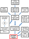 |
Fig. 1. Forward-modelling of the X-GAP selection. We started from a dark matter halo light cone generated from the Uchuu simulation, built a novel method for assigning cluster and group X-ray profiles and temperatures as a function of the halo mass and redshift, and used abundance-matching schemes to simulate galaxies and AGN. We generated X-ray events and accounted for the telescope response. Finally, we reproduced the detection schemes in X-ray and optical bands to select an X-GAP-like sample from our simulation. |
We develop a novel method to populate haloes with X-rays from galaxy clusters and groups (see Sect. 3) and implement the AGN model from Comparat et al. (2019). We model the diffuse X-ray background following the real ROSAT background maps (Snowden et al. 1997). We generate X-ray events using the SIXTE software (Dauser et al. 2019). We detect sources in the X-ray and optical bands and cross-matched the output galaxy cluster and group catalogue to the input dark matter haloes. The whole process is detailed in the next sections.
2.1. Halo light cone
Uchuu is a large dark matter only simulation with high resolution (Ishiyama et al. 2021). It is based on a standard Flat ΛCDM cosmology with parameters from Planck Collaboration VI (2020). Individual snapshots are publicly available4. The box size is 2 Gpc/h, with a total of 2.1 trillion particles, for a mass resolution of 3.27 × 10⁸ M⊙/h. The gravitational softening length is 0.4 kpc/h. This is ideal for our purpose to minimize cosmic variance effects due to the all-sky X-ray selection, but also to properly account for faint local galaxies in the SDSS optical selection. Haloes are identified with the Rockstar-Consistenttrees algorithm (Behroozi et al. 2013), based on a FoF approach in six dimensions for positions and velocities. The parallel processing of multiple snapshots provides a consistent halo catalogue as a function of redshift. We concatenate individual snapshots into a halo light cone by adapting the methodology of Comparat et al. (2020) to match the geometry of Dong-Páez et al. (2024). We combine snapshots at redshift 0.0, 0.09, 0.19, 0.30, 0.43, 0.49, 0.56, 0.70, 0.78, 0.86, 0.94, 1.03, 1.12, 1.22, 1.32, 1.43, 1.54, and 1.65 to obtain a smooth redshift distribution of dark matter haloes. This allowed us to include the bulk of the AGN population detected in the ROSAT All-Sky Survey (RASS), which peaks at redshift 0.3 and has a long tail extending just above redshift 1.5 (see e.g. Anderson et al. 2007). A rotation of 10 deg in the x-z cartesian plane allowed us to match our coordinates to the geometry of the UchuuSDSS simulation, for the observer placed in the origin, providing the same conversion between cartesian to angular coordinates. We convert cartesian coordinates into equatorial coordinates according to
 (1)
(1)
where the conversion from ϕ to RA is done in python with the numpy.mod function (van der Walt et al. 2011). We infer the cosmological redshift zcosmo from the comoving distance dC using astropy (Astropy Collaboration 2013) and add the effect of peculiar velocities according to:
 (2)
(2)
where c is the speed of light and zspec is the idealised spectroscopic redshift. Note that in Eq. (1) we place the observer in (0,0,0). The box is replicated 8 times around the origin by shifting all combinations of each cartesian coordinate by one box length. In the construction of the light cone we use the output of a given snapshot at redshift zsnap according to (zsnap−1+zsnap)/2<z<(zsnap+zsnap+1)/2. For z>0.78 the comoving distance to the edge of the snapshot becomes larger than the box length. Therefore, we replicate the snapshots one more time along each direction, obtaining 64 replicas around the observer at the origin for snapshots between z = 0.78 and z = 1.65.
We then query subhalo members for each distinct halo and use the individual peculiar velocities to compute the true halo line of sight velocity dispersion, according to:
 (3)
(3)
where Nmem is the number of subhaloes for each distinct halo. We restrict our measurement to subhaloes with virial mass larger than 9.3 × 10⁹ M⊙. It allowed us to resolve these structures with more than 20 particles, so that Rockstar provides secure (sub)halo properties (Knebe et al. 2011, 2013). In addition, it allowed us to describe SDSS-like galaxies with stellar masses down to 108 M⊙, the lower limit in the GALEX-SDSS-WISE Legacy Catalog (GSWLC, Salim et al. 2016). We verified the robustness of the measured true velocity dispersion by increasing the threshold to 50 and 100 particles, hence increasing the subhalo resolution level at the cost of reducing the number of subhaloes used in Eq. (3) (Onions et al. 2012), and did not find significant differences in the estimate of velocity dispersion. For computational power reasons, we compute velocity dispersions only for haloes in the first two redshift snapshots, meaning that we can access intrinsic halo velocity dispersion in our light cone up to z≤0.14. Therefore, we miss it for haloes present in the optical mock for z>0.14, but we are not affected by this limitation thanks to the upper limit of X-GAP at z = 0.06, allowing us to focus on lower z when modelling the selection function.
Various versions of UchuuSDSS are available, depending on the geometry and the conversion between cartesian and angular coordinates. By placing the observer in the origin of the boxes, we obtain a dark matter halo light cone with coordinates matching the UchuuSDSS0 galaxy mock from Dong-Páez et al. (2024). A slice of the full light cone is shown in Fig. 2, where the LSS expands from the origin as a function of the comoving distance to the observer. Each halo is colour-coded by its redshift (see Eq. (2)) and the shaded areas denote the intervals corresponding to the output from different snapshots. In addition, we rotate and flip the coordinates to match the geometry of three additional light cones with the observer at the same place, allowing us to independently reproduce the SDSS sky footprint of 7261 deg2 with four different regions, corresponding to the UchuuSDSS mocks from 0 to 3. In the rest of the article we will refer to the combination of the four light cones when stating our results. When needed, we assign hydrogen column density due to galactic absorption following HI4PI Collaboration (2016).
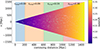 |
Fig. 2. Dark matter halo light cone generated from individual Uchuu snapshots. This panel shows a slice within ±50 Mpc along the z-axis up to redshift of 0.4. We show haloes more massive than 1012.5 M⊙ colour-coded by its redshift. The shaded areas denote the various snapshots we used to generate the light cone. |
2.2. Active galactic nuclei
We populate dark matter haloes from the Uchuu simulation with AGN using the model from Comparat et al. (2019). It is based on a halo abundance matching scheme (HAM) between stellar and halo mass. We select haloes with virial mass larger than 1011 M⊙. The stellar masses are assigned to each halo based on the stellar to halo mass relation from Moster et al. (2013), which accounts for the intrinsic scatter in the relation. The model is calibrated to reproduce the AGN duty cycle and the hard X-ray luminosity function (see Georgakakis et al. 2017; Aird et al. 2015). The choice of the 2–10 keV band is particularly useful because the hard band flux is less affected by the AGN spectra and obscuration properties compared to a softer X-ray band. The model produces an AGN population that matches measurements of the evolution of their number density with redshift and luminosity, and the clustering properties (Georgakakis et al. 2019). Various works in the literature reported the identification of a soft excess feature in AGN spectra (Boissay et al. 2016; Ricci et al. 2017; Waddell et al. 2024), which we include in our modelling. We assume a typical spectrum composed by an absorbed power-law with photon index equal to 1.9, with the addition of a scatter component from cold matter with 2% normalisation (Yaqoob 1997), and a reflection one with emission lines (Nandra et al. 2007). We add a phenomenological 0.2 keV thermal bremsstrahlung component to model the soft excess (Boissay et al. 2016). We generate model spectra with Xspec (version 12.13.1, Arnaud 1996), our model reads TBabs(ztbabs(powerlaw + constant × bremss) + constant × powerlaw + pexmon × constant). We assign the spectra by a nearest neighbour search in redshift, intrinsic absorption, and galactic extinction. We simulate AGN down to an X-ray flux of 10−13.2 erg/s/cm2, slightly below the flux limit of the ROSAT all sky survey (Voges et al. 2000). This allowed us to simulate the AGN population corresponding to the one detected in the real RASS, but without double counting the faint, undetected AGN contributing to the cosmic X-ray background (see next Section). Indeed, in the most recent processing of the ROSAT All-Sky Survey, that is, the Second ROSAT all-sky survey (2RXS) source catalogue by Boller et al. (2016), we find that the 1st percentile of the cumulative flux distribution calculated assuming a power-law spectrum appropriate for AGN corresponds to a flux of approximately 5.8 × 10⁻¹⁴ erg/s/cm2. Given the uncertainties associated with flux measurements at these faint levels, which are sensitive to the assumed spectral model, we consider this threshold to be broadly consistent with our adopted flux cut of 10−13.2 erg/s/cm2.
2.3. X-ray background
We merge the individual band 4–7 RASS background maps (Snowden et al. 1997)5 into a single map in the 0.44–2.05 keV band, summing the count rates from each individual band. This strategy accounts for spatial variations of the X-ray background, including the emission of the eROSITA bubble (Predehl et al. 2020) in the sky covered by SDSS, which was already detected in the RASS as the North Polar spur (Egger & Aschenbach 1995). Its brightest part is in the galactic plane (Willingale et al. 2003). We model the background assuming three main components: unabsorbed plasma emission from the local hot bubble (LHB), absorbed plasma emission from the galactic halo (GH), and the cosmic X-ray background (CXRB) from undetected point sources. In Xspec terms our model reads APEC + Tbabs × (APEC + powerlaw). We assume solar abundance (Z⊙) and kT = 0.097 keV for the LHB, 0.3 Z⊙ and kT = 0.22 keV for the GH, and a photon index Γ = 1.46 for the CXRB. We stress that the faint AGN population is not simulated as individual sources (see previous Section), because its emission is already present in the background maps. The proportional counter PSPC of ROSAT has low sensitivity to high energy particles and soft protons, therefore we neglect the particle induced background component in our spectral model. Indeed Eckert et al. (2012) demonstrated that the PSPC instrumental background is more than one order of magnitude lower than the sky background. We process the merged map into HEALPix6 format with NSIDE = 64, generating 49 152 areas of about 0.84 deg2. We convert the count rate to flux using the spectral model defined above folded with the ROSAT PSPC response file and integrate it in the individual areas to obtain the total flux from each pixel in the energy band of interest.
2.4. Event generation
To generate X-ray photons we use the SIXTE software (Dauser et al. 2019). It is an end-to-end X-ray simulator that allowed a forward-modelling of observations that accounted for vignetting, the energy-dependent PSF, the ancillary response file (ARF), and the redistribution matrix file (RMF). We built an ad hoc SIXTE module to simulate the RASS data. We use publicly available response files from ROSAT7. We build an analytical PSF model following the work from Boese (2000) (see Eq. (6), (7) therein). The ROSAT PSPC has a sensitive area of 8 cm diameter (Pfeffermann et al. 1986). The total area is A=π×(d/2)2, corresponding to a mock pixel with a size of  mm on a side. During the readout, we ignore any correction between pulse height amplitude and channels, as the time resolution of proportional counters is very good. We account for a dead time interval after each event of 180 μs, when the detector is not sensitive to radiation. We collect information about the telescope pointing from the publicly available ancillary ROSAT data8. We concatenate each file to generate a single RASS attitude file describing the coordinate pointing and the roll angle of the telescope as a function of time. We ignore time spans with operational problems (see Table 2 in Voges et al. 1999). For processing purposes, we divide the area covered by the X-GAP sample into 627 pixels of about 53 square degrees using healpix with NSIDE = 8. For clusters and groups, we generate idealised input images following the ellipticity of each dark matter halo, which SIXTE used to simulate events from extended sources on the plane of the sky.
3. Model of clusters and groups
Since the Uchuu simulations contain only dark matter, we need a prescription to populate the haloes with baryons. Various implementations exist in the literature, such as semi-analytical models (Shaw et al. 2010; Osato & Nagai 2023), or phenomenological approaches based on real observations (Zandanel et al. 2018), also accounting for covariances between different observables (Comparat et al. 2020). We proceed in this direction and develop a new model to predict the X-ray emissivity profile and temperature as a function of halo mass and redshift using a machine-learning approach. Our method builds on Comparat et al. (2020) and aims to predict cluster and group properties with the correct covariances. The Comparat et al. (2020) model is based on high signal to noise observation of massive galaxy clusters and required ad hoc corrections in the galaxy group regime (see discussion in Seppi et al. 2022). Although hydrodynamical simulations are not a perfect reconstruction of the real Universe due to various assumptions, for example, in the feedback and star formation prescriptions, they still provide a complete view of the galaxy group population under those assumptions. On the one hand, our new model is more reliable at low masses <1014 M⊙, because it is informed by hydrodynamical simulations, which do not lack objects in this mass range. On the other hand, hydrodynamical simulations cannot consistently predict hot gas properties for galaxy groups (Eckert et al. 2021). However, our definition of the selection function in terms of observables makes our modelling less dependent on specific models assumed in the implementation of baryonic physics (see also Appendix A). Similarly, various prescriptions for the hot X-ray gas may change the total number of sources as a function of X-ray observables at fixed optical properties in our framework. However, the selection function is a ratio, and it is not dependent on a given X-ray model if it also accounts for optical properties in its definition (see Sect. 5). We introduce the concepts, the model, and show the results about inferred observables in this section.
3.1. Emission measure profiles
We use the emission measure integrated along the line of sight to model the profiles. This quantity is also known as emission integral and should not be confused with the volume integrated emission measure (Eckert et al. 2016). When mentioning the emission measure, we refer to the one integrated along the line of sight. At radius x=r/r500c it can generally be deduced from the X-ray surface brightness (Neumann & Arnaud 1999; Arnaud et al. 2002). It is defined as follows:
 (4)
(4)
where S(E) is the detector effective area at energy E, σ(E) is the absorption cross section, fT((1+z)E) is the emissivity in cts/s/keV × cm3 for a plasma of temperature T.
In practice, various works in the literature use a conversion factor between count rate and APEC normalisation with xspec to obtain the emission measure profile from surface brightness. It allowed us to account for the response of the instrument (Pratt et al. 2009; Eckert et al. 2012; Bartalucci et al. 2023). More details are given in Appendix D. The self similar scaled emissivity profile is finally obtained as follows (see e.g. Arnaud et al. 2002; Eckert et al. 2012):
![Mathematical equation: $$ EM_{\mathrm {SS}}(x) = EM(x) \left [\frac {kT}{10\,{\mathrm {keV}}}\right ]^{-1/2} E(z)^{-3}. $$](/articles/aa/full_html/2025/07/aa53977-25/aa53977-25-eq6.gif) (5)
(5)
3.2. Profile extraction from TNG
We train a neural network on galaxy clusters from the hydrodynamical TNG300 simulation9 (Nelson et al. 2019). The box size is 205 Mpc/h and the dark matter particle mass is 5.9 × 10⁷ M⊙/h, therefore galaxy groups and clusters are simulated with extremely high resolution. We use groups and clusters with M500c > 8 × 10¹² M⊙ at snapshots corresponding to z = 0.01, 0.03, 0.06, 0.1, 0.2, 0.3, 0.5, 1.0, 1.5. In the snapshot at z = 0.03, which is within the X-GAP window, we model 4101 objects.
Following a methodology similar to Shreeram et al. (2025), we retrieve the data stored for each gas cell and model its emission measure using pyxsim (ZuHone et al. 2015), which provides a Python interface to the PHOX code (Biffi et al. 2012, 2013). We consider gas cells with temperature between 0.1 and 20 keV, with gas density below 5 × 10⁻²⁵ g/cm3. We project the 3D model of each cell along the x cartesian direction and integrate them within circular apertures to retrieve the emission measure profile integrated along the line of sight (as defined in Eq. (4)).
Next, we need an estimate for the source temperature in the simulation. Although computing the local temperature of a gas cell or particle in hydrodynamical simulations is possible using the internal energy, translating a large amount of individual temperatures into a global halo temperature is not trivial, as it often requires the assumptions of weights for different gas properties, which may result in disagreements between outputs from hydro simulations and observations (Mazzotta et al. 2004; Rasia et al. 2005, 2014). In observations, the temperature measurements comes rather from fitting the source spectrum with a single global temperature. Therefore, to be as close as possible to an ideal X-ray temperature from the observations’ perspective, we generate an ideal spectrum starting from the emission measure profile. We determine the photon X-ray emissivity using an APEC model (Smith et al. 2001) as a function of density and temperature of each gas cell, assuming a metallicity of Z = 0.3 Z⊙ and the abundance table from Asplund et al. (2009), using the emissivity of each cell as a distribution function for photon energy, assuming a large collective area of 10 000 cm2 and a long exposure time of 500 ks. We infer the ideal X-ray halo temperature by fitting the resulting global spectrum with an APEC model in Xspec, fixing the redshift to the redshift of the TNG snapshot and metallicity to 0.3, while leaving temperature and normalisation free to vary. The result is a collection of clusters and groups with mass, redshift, emission measure profile, and temperature. The assumption of Z = 0.3 Z⊙ is reasonable for the average metallicity in galaxy groups, especially outside the core (Sun et al. 2009; Mernier et al. 2017; Bahar et al. 2024). For detailed comparisons between the prediction of hydrodynamical simulations and the real X-GAP, accounting for the metallicity distribution along the group profile may also help in shedding light on AGN feedback prescriptions and we will consider it in future work.
3.3. Profile generation with machine-learning
The field of machine-learning and neural networks has enormously grown in recent years, with a multitude of implementations for various algorithms, such as variational auto encoders (Kingma & Welling 2013), and generative adversarial networks (Goodfellow et al. 2014). Different works in the literature have successfully applied machine-learning techniques in astronomy, for example to study galaxy cluster morphologies (Benyas et al. 2024), predict galaxy cluster masses (Ntampaka et al. 2019; Krippendorf et al. 2024), infer the gravitational potential of the Milky Way (Green et al. 2023), and study dark matter simulations (Rose et al. 2025).
In this context, normalising flows have emerged as a popular way to model and generate data (Hahn & Melchior 2022; Li et al. 2024; Crenshaw et al. 2024). normalising flows constitute a machine-learning approach to construct a complex probability distribution from a set of transformations of simple distributions (see Kobyzev et al. 2019, for a review). Given a set of observed variables  the goal is to model its probability distribution
  , by starting from a continuous random variable
  that follows a simple probability distribution
  , for instance a Gaussian one. The idea is to transform the simple
  into a more complex one through a collection of N invertible and differentiable functions (bijectors)
  . The transformed probability distribution is:
 (6)
(6)
where  and
and  is the Jacobian of each transformation fi. The variable y flows through the bijectors chain, while the Jacobians normalise the probability distributions of the transformed variable. The training process of a normalising flow consists of optimising the parameters of the bijectors in the chain to best reproduce the probability distribution of the observable
  . During training we minimize the negative log likelihood defined from Eq. (6) as follows:
![Mathematical equation: $$ \log {\cal {{L}}} = \sum _{\mathrm {i = 0}}^{\mathrm {N}} \log p_{\mathrm {y}}[f^{-1}_{\mathrm {i}}({\bar {x}})] + \sum _{\mathrm {i = 0}}^{\mathrm {N}}\log | \det Df_{\mathrm {i}}({\bar {x}}) |, $$](/articles/aa/full_html/2025/07/aa53977-25/aa53977-25-eq17.gif) (7)
(7)
because for bijectors the determinant of the product of the jacobian matrices of each transformation is the product of the individual determinants.
Our model is based on a multivariate normal distribution with the same dimension as our training dataset. Then we create an autoregressive normalising flow (MAF, Papamakarios et al. 2019) using autoregressive models for density estimation (MADE, Germain et al. 2015). They describe the final probability distribution as the product of conditional probabilities:
 (8)
(8)
where D is the number of dimensions of a given dataset. In particular, each component of the observable  is predicted by transforming the latent variable
  with a shift μi and a rescale factor σi that depend on the previous components:
 (9)
(9)
This set-up makes the calculation of the Jacobian in Eq. (6) simple, which reduces for each component to
 (10)
(10)
Finally, we minimize the negative of the log likelihood in Eq. (6) by the gradient descent method using the Adam optimiser with a learning rate of 10−3. One of the caveats in the field of computer vision is that the MAF architecture is slow in generating new data, because the generation of each variable needs all the previous inputs in the flow. Given the size of the dataset we need to generate we are not affected by this limitation.
In this study, we develop a network to predict the self similar emission measure profile (see Eq. (5)) and X-ray temperature, conditionally on mass and redshift. This allowed us to generate X-ray quantities (i.e. profiles and temperatures) using prior information of mass and redshift from our Uchuu halo light cone. Together with the profiles extracted from TNG, in the training set we add the HIFLUGCS sample (Reiprich & Böhringer 2002), and Chandra observations of SPT-selected clusters from Sanders et al. (2018). They make the prediction of our model more robust at high mass, where only a few haloes are available in TNG. If the X-ray data is not sufficient to reach the halo outskirts, we follow the approach of Comparat et al. (2020) and extrapolate the profile using a power law whose slope is fitted on the three outermost bins. The input dimension of our network is equal to 2 (M,z), while the output dimension is equal to 21, that is, 20 radial bins logarithmically spaced between 0.02 and 3 R500c plus one value for temperature. In contrast to temperature, the values of mass and surface brightness span many orders of magnitudes. Therefore, we model their log-value and normalise each array in our training data, so that the network only needs to work with numbers between 0 and 1. We then apply the inverse transformations to convert the output values of the network to predictions in physical units. We apply a median smoothing to the radial profiles. This technique replaces points that exhibit strong fluctuations relative to their neighbors with the median of the two preceding and two following points along the profile, effectively preserving the overall shape and slope of the profile. We build model with TensorFlow (Abadi et al. 2015), it is composed of three MAF. Each autoregressive network has two output parameters (μi,σi), two layers of 128 units each, and a sigmoid activation function. We train the model for 200 epochs, with a batch size of 16. We find that this set-up reproduces well the distributions of observed clusters and group properties compared to existing observations, as shown in the next section. This model does not introduce a correlation between the X-ray morphology (cool core or non-cool core) and the dynamical state of the dark matter haloes (see e.g. Seppi et al. 2021). The X-ray detection scheme is designed to be insensitive to the relaxation state of the hot gas and we verified that this is the case in Sect. 7.1.
3.4. Results
Starting from the halo masses and redshifts in the Uchuu light cone, we use the trained neural network to generate profiles and temperatures for each dark matter halo. The result is shown in Fig. 3. It displays the self similar scaled emission measured profiles, colour-coded by temperature. The scaling of the profiles with temperature is clear and as expected: hot clusters exhibit high surface brightness with steep profiles, while cooler systems show lower normalisation and flatter slopes. Specifically, we observe a correlation between emission measure and temperature in the central region within 0.5 × R500c, and a more uniform distribution of the profiles towards the outskirts (Eckert et al. 2012). Our result is in agreement with Comparat et al. (2020), which was built to reproduce observations of massive clusters by construction, and the profiles of X-COP clusters (Ghirardini et al. 2019). The bottom part of the panel shows the intrinsic scatter of the profiles at different radii. It is defined as the 16th–84th percentile distribution of the profiles around their median. It is the only scatter component, as the ideal model has no noise for individual systems. It is compared to the model from Comparat et al. (2020). The intrinsic scatter is computed on the overall population, so the halo selection is different between the lines shown in the bottom panel of Fig. 3. Nonetheless, we find overall a good agreement between the prediction of our neural network to previous models and observations. Our model predicts a slightly smaller intrinsic scatter compared to the training set in inner region, with a value of 0.39 against 0.48 at 0.1 × R500c. The opposite holds in the outskirts, with values of 0.7 and 0.55 at 2 × R500c. However, the model prediction and the training set are always compatible within 1σ throughout the whole profile.
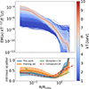 |
Fig. 3. Emission measure profiles with self-similar scaling, colour-coded for temperature, as a function of radius in units of R500c. The units on the y-axis are Mpc keV−1/2 cm−6. The bottom part of the panel shows the evolution of the intrinsic scatter of the profile at different radii. For reference, it is compared to the model from Comparat et al. (2020) and profiles of X-COP clusters (Ghirardini et al. 2019). |
We compute the value of X-ray luminosity with a cylindrical integral of the emissivity profile as follows:
 (11)
(11)
where r is the radius and Λ(kT) is the temperature dependent cooling function in the 0.5–2.0 keV band in units of cm3 erg s−1 (Sutherland & Dopita 1993). For convenience, we tabulate the cooling function on a fine grid of temperature (every 0.075 keV) and interpolate. We apply a 2D K-correction to convert intrinsic luminosities to the observer frame. We tabulate conversion factors as a function of cluster temperature and redshift. Finally, we additionally account for galactic absorption. We compute the galactic gas column density (NH) at the angular position of each cluster using the maps from HI4PI Collaboration (2016). Similarly to the cooling function case in Eq. (11), we tabulate the conversion factors and then interpolate at the exact values of luminosity, redshift, and NH of each cluster.
To assess the robustness of the model, we compare the scaling relations between observables and halo mass to literature results. The results are shown in Fig. 4, displaying the X-ray luminosity to mass and temperature to mass relations. Overall, we find good agreement between our result and observations. The model predicted by the neural network applied to the Uchuu light cone is in blue, and it is compared to a collection of real clusters and groups, including a RASS selected groups sample (Lovisari et al. 2015), some ROSAT selected sample of massive clusters (Mantz et al. 2016; Schellenberger & Reiprich 2017), the XMM-XXL survey (Adami et al. 2018), some Sunyaev-Zeldovich (SZ) selected samples in the radio/millimeter bands from SPT (Bulbul et al. 2019) and Planck (Lovisari et al. 2020), and the eROSITA catalogues from eFEDS (Liu et al. 2022a) and eRASS1 (Bulbul et al. 2024; Seppi et al. 2024). The bottom part of both panels shows the intrinsic scatter evolution as a function of halo mass. For the LX−M500c relation we find a slope of 1.58 ± 0.02. It is steeper than the self-similar model expectation of 4/3, because the gas fraction in the galaxy group regime is smaller than the cosmic one, which reduces luminosity at fixed mass. Our model aligns well with previous observations. The luminosity at fixed mass is slightly higher than the eRASS1 sample, likely due to software and calibration differences (see discussion in Bulbul et al. 2024). In any case, an accurate and precise comparison is not possible since for some of these observational samples a full scaling relation model including systematics and selection function is not available. In addition the masses have been computed using different techniques, such as weak lensing calibration, hydrostatic equilibrium assumption, or scaling relations, which means that the observational samples have different accuracy and precision along the x-axis in Fig. 4. The scatter in luminosity predicted by the neural network evolves for different masses, from about 0.4 dex at about 2 × 10¹³ M⊙ to 0.3 dex at 8 ×10¹⁴ M⊙, with a median value of 0.31 dex. This is in agreement with expectations when comparing these values with observations, given the fact that our model does not include measurement uncertainties that affect the latter. Literature values span between 0.2 and 0.4 (Lovisari et al. 2015; Bulbul et al. 2019; Sereno et al. 2019; Seppi et al. 2024). The relation is flatter in the mass range between 1 × 10¹³ and 5 × 10 13 M⊙. This is intrinsic to the TNG simulation, as indicated by the dashed magenta line, which reports the TNG100 prediction as shown in Zhang et al. (2024). This effect could be due to line cooling. At fixed density, the X-ray emissivity is enhanced for temperatures around 1 keV due to the addition of line cooling on top of the self-similar expectation of thermal bremsstrahlung. Indeed Lovisari et al. (2021) showed that the emissivity quickly increases by up to a factor of about two in the temperature range of 1 keV, this holds for different metallicities and energy bands. Disentangling such an effect from the reduced gas fraction in groups compared to clusters and the variation of the gaseous atmosphere due to AGN feedback is not trivial. In any case, we verify that this is not a limitation for our purpose of formulating the selection function in terms of observables. We reduce the luminosities extracted from the cluster model by a constant factor of 10%, that is, the fluxes are rescaled by a factor of 0.9. We re-generate the SIMPUT cluster files for the mock number three and process it with our end-to-end approach. We find that the final detection probability as a function of flux is in excellent agreement with the main work combining the four light cones. In addition, the X-GAP flux limit is about 5 × 10⁻¹³ erg/s/cm2, where we find an excellent agreement between different mocks and the test with rescaled luminosities. We further elaborate in Appendix A.
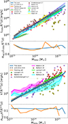 |
Fig. 4. X-ray scaling relation prediction of the cluster and group model. Top panel: Scaling relation between X-ray luminosity obtained by integrating the emission measure profiles (see Eq. (11)) and halo mass. Bottom panel: Scaling relation between temperature and halo mass. The blue shaded area shows the 16th–84th percentile distribution for the model applied to the Uchuu light cone in each mass bin. Our model is compared to a collection of real groups and cluster samples. The bottom part of both panels shows the intrinsic scatter evolution as a function of halo mass. |
For the TX−M500c relation we find a slope of 0.63 ± 0.02, close to the self similar model expectation of 2/3. The scatter is fairly constant as a function of mass, with values around 0.13. This is larger compared to the model from Comparat et al. (2020), reporting values around 0.07. Results from observational studies span from 0.05 (Lovisari et al. 2020), 0.064 (Sereno et al. 2019), 0.069 (Chiu et al. 2022), to 0.18 (Bulbul et al. 2019).
4. Catalogue creation
We follow the selection scheme devised by Damsted et al. (2024) for AXES, the successor of CODEX (Finoguenov et al. 2020), and the parent sample of X-GAP (Eckert et al. 2024). The optical FoF detection follows Tempel et al. (2017). On top of the positional matching between X-ray and optical detections, we add a matching to the input clusters and groups, which allowed us to quantify completeness and purity levels in the AXES catalogues. The whole procedure is detailed in this section.
4.1. X-ray detection
We run a wavelet source detection algorithm, as introduced by Vikhlinin et al. (1998). It consists in convolving the image with a kernel with a positive core and a negative outer ring, allowing the isolation of objects with a given angular size. The kernel is a Mexican hat function. This allowed us to subtract the background accurately because the convolution of the kernel with any local linear function is zero (see Vikhlinin et al. 1998, for details). The wavelet scale n is defined such that the outer scale corresponds to a Gaussian with size of 2n−1 pixels. We follow the implementation described in Käfer et al. (2019). We divide the detection of point-like emission using wavelet scales of 2, 3, and 4 pixels; from the detection of extended-like emission using wavelet scales of 5 and 6 pixels. A key step at this point is using images with the same pixel size as the real RASS maps, because this is the scale at the base of the wavelet filters. Given the pixel size of 45 arcsec, these scales correspond to 1.5, 3, and 6 arcmin for point-like emission, and 12, 24 arcmin for the extended-like case. Given the redshift range of X-GAP, using such large angular scales allowed us to create a source catalogue that was only sensitive to the baryonic content of groups in the outskirts. For a typical 5 × 10¹³ M⊙ group at z = 0.04, R500c covers about 12 arcmin. This minimizes the impact of AGN feedback, mostly evident in the central region, on the sample selection. The centre of X-ray emission is located by running SExtractor (Bertin & Arnouts 1996) on the sum of the extended source wavelet images.
4.2. Optical detection
Our optical mock is based on the UchuuSDSS simulation (Dong-Páez et al. 2024). The UchuuSDSS catalogues are publicly available10. They are based on a subhalo abundance matching (SHAM) between the maximum value of the halo circular velocity, serving as a stellar mass proxy, and a target luminosity to match the SDSS galaxy luminosity function. They add a smoothing to reproduce the observed redshift trend of the luminosity function and assign colours based on empirical models. Apparent r-band magnitude (mag-r) are computed accounting for colour-dependent k-corrections. Finally, they assign additional galaxy properties, such as stellar mass and star formation rate, by a nearest neighbour search within SDSS. The authors demonstrated that this approach recovers SDSS population properties by construction, such as the stellar mass function, galaxy clustering, redshift distribution, and colour magnitude diagrams (see Dong-Páez et al. 2024, for more details).
The optical FoF algorithm from Tempel et al. (2017), used in Damsted et al. (2024) and in this work, only requires angular coordinates, redshift, and mag-r. We treat their catalogue as the mock corresponding to the real galaxy SDSS data used in FoF search of galaxy groups. We select galaxies with redshift z<0.2 and r-band magnitude r−mag<17.77 to reproduce the same selection as Tempel et al. (2017). The authors used a redshift dependent linking length according to:
![Mathematical equation: $$ d_{\mathrm {LL}}(z) = d_{\mathrm {LL,0}}[1 + \arctan (z/z_\ast )], $$](/articles/aa/full_html/2025/07/aa53977-25/aa53977-25-eq24.gif) (12)
(12)
with dLL,0 = 0.34 Mpc and z* = 0.09. The original SDSS catalogue contains 584 449 galaxies and 88 662 groups with at least two members. In the four simulations we used there are 624 639, 610 845, 595 183, and 626 333 galaxies. Differences between the mocks are attributed to cosmic variance. These numbers are higher compared to the real Universe observed in SDSS. This is due to an overestimation of the galaxy density in the optical mock compared to the real SDSS at redshift close to 0.2, as pointed out in Dong-Páez et al. (2024). This is not a limitation in our redshift range of interest z<0.14, where we also have access to velocity dispersions (see Sect. 2.1). In fact, in this range the mocks contain 484 960, 473 439, 456 510, 492 000 galaxies compared to 464 978 in the real SDSS. We discard groups with fewer than five galaxy members, as their properties are hard to measure quantitatively (replicating the selection of Damsted et al. 2024). In addition to the catalogue of FoF groups, the algorithm from Tempel et al. (2017) provides the catalogue of member galaxies assigned to each FoF group. We use the latter for matching the FoF groups to input dark matter haloes, as explained in the next section.
We further clean our optical catalogue following the same approach as Damsted et al. (2024) and apply the CLEAN algorithm (Mamon et al. 2013). It minimizes the impact of interlopers, that is, galaxies falling within the projected virial radius but that are actually located outside the main halo, by selecting member galaxies based on their position in the phase space of radial distance from the centre and rest frame velocity. An iterative process based on an NFW model estimates r200c from velocity dispersion. Then the algorithm selects galaxies within the ±Kσlos(R), with K = 2.7. For more details about the theoretical formalism of CLEAN, we refer the reader to Appendix B in Mamon et al. (2013). Finally, using the cleaned members, we compute observed velocity dispersion using the Gapper method (Beers et al. 1990), an estimator based on the gaps between ordered measurements: it sorts the values of individual velocities and uses the difference between velocity intervals as weights to compute the final velocity dispersion (Wetzell et al. 2022). The uncertainty on the measurement is computed as the standard deviation of 1000 bootstrap resamples.
4.3. Matching input and output
Given the set-up of our simulation, we need to perform a three-way matching, between dark matter haloes in the light cone, detections in the X-ray mock, and FoF optical groups. For a given dark matter halo, we can ask whether it is detected in the X-ray, optical, or both mocks. For the matching procedure we focus on haloes at z≤0.14, where we measured input velocity dispersions. We ignore optical detections in the range between 0.14 and 0.2, which is nonetheless outside the X-GAP range of interest.
4.3.1. X-ray to haloes
We follow a similar scheme to Seppi et al. (2022) to match input and output catalogues from the X-ray point of view, and use the information stored in the unique ID of each photon. For each event, the ID encodes the source responsible for the emission, either a cluster, an AGN, or the background. For each entry in the wavelet catalogue, we query all the events within a radius of 6 arcmin. We assign such detection to the simulated source emitting the majority of the photons. If different sources provide the same exact amount of events, we give priority to the input cluster. We only account for input sources providing more than two events on the mock detector, and sources providing an amount of events larger than the 0.8 percentile point of the Poisson distribution with mean value equal to the total number of counts provided by the background within the given aperture of 6 arcmin (see also Liu et al. 2022b, for a similar implementation).
The main difference compared to previous work about eROSITA simulations cited above is that in this case we are particularly interested in the detection of extended sources rather than contamination. Indeed, it is clear from the X-GAP data that contamination from AGN is not an issue (Eckert et al. 2024), with only one false detection out of 49. Therefore, if a detection contains cluster emission but is not assigned to the cluster directly, that is, due to the presence of a bright AGN, we still consider the cluster as detected. Indeed, the cross-match with the optical mock allowed us to clean the otherwise contaminated X-ray classification of such sources. However, we track all cases of sources whose emission is contaminated by a secondary object. To do this, we require that the amount of counts provided by the secondary source within the given aperture is larger than the square root of the counts produced by the primary match.
4.3.2. Optical to haloes
We now search for an optical FoF counterpart to each simulated halo. We start from the input halo catalogue and search for optical matches in radial angular apertures of 3×R500c in the RA-Dec plane. We then query the candidate matches, if present, and keep only the ones with a relative redshift error below 1%, that is,  . This threshold is comparable to state of the art results on cluster photometric data (see e.g. Kluge et al. 2024), and thus serves as a reasonable upper limit that also accounts for additional observational redshift uncertainties. We perform the matching in redshift space, that is, ztrue includes peculiar velocities (see Eq. (2)), which help to disentangle close pairs or mergers due to the fact that the optical detection uses observed redshifts as well. For each candidate we evaluate the matching quality by computing a matching statistic accounting for a mass probability, encoded in the estimate of velocity dispersion, and a distance probability, related to the 3D cartesian distance from the true halo centre. The matching statistic is therefore higher if the optical candidate is well centred on the true position of the halo, and if velocity dispersion is accurately estimated. The final equation reads:
 (13)
(13)
where  is a log-normal function describing the measured velocity dispersion σv,M that is centred around the true value σv,T. We use a log-normal scatter of σLN = 0.08 dex. An accurate refinement of this quantity is provided in Sect. 6.
We consider the optical FoF object with the highest matching statistic as the primary match to an input halo, if more than one candidate is present. Although this set-up easily allowed us to state whether a halo is detected or not, it may assign the same optical FoF object to different input haloes. In such cases, we assign the primary match to the halo whose FoF object has the highest matching probability. For the other haloes, we then check if they have secondary matches. If the secondary matches have not been assigned as primary matches to another halo, we upgrade them to primary matches. Otherwise, we mark the cluster as blended with another primary detection. With this method we now have a unique way of mapping input haloes into FoF optical groups and clusters.
An example of the end result of the processing detailed in this section is shown in Fig. 5. It is a field of one square degree with one of the brightest clusters in our simulation. X-ray photons generated by various components (clusters and groups, AGN, background) are shown as small dots (in blue, orange, green). Galaxies are displayed by the plus signs and represented according to their g-r colour. True halo positions (wavelet detections, optical FoF detections) are located at the large crosses (cyan circles, magenta triangles). In this case, the bright system in the centre of the image is properly detected both in X-ray and optical bands. In addition, a fainter nearby halo is found by the optical FoF algorithm, but not in the wavelet processing.
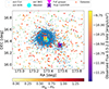 |
Fig. 5. Image example showing one of the brightest clusters in our mock with the additional components we included in the simulation. A secondary halo is located in the south-east region compared to the brightest one. The events generated by clusters (AGN, the X-ray background) are displayed as small dots in blue (orange, green). The true halo position is shown with large crosses, colour-coded by the X-ray flux. The position of the X-ray wavelet (optical FoF) detection is located at the cyan circle (magenta triangle). Each galaxy is marked by the small plus signs, according to their g-r colour. The vertical colour bar refers to input groups and clusters (the large crosses), the bottom one to individual galaxies (small plus signs). |
We generate X-ray photons for a total of 62 868 clusters and groups below redshift 0.14, with flux larger than 10−14 erg/s/cm2. This limit is much below the expected RASS detection limit (Böhringer et al. 2000; Ebeling et al. 2001). Between them, 17 669 are detected in the optical mock, for an optical completeness of 28.1%. In the X-ray mock, the wavelet processing identifies 5589 sources, for an X-ray completeness of 8.8%. After combining X-ray and optical detections, we obtain 3975 sources, for a global completeness of 6.3%. When focusing on a lower redshift slice, or more massive systems, the detection probability increases. In the redshift range of interest for X-GAP, between 0.02 and 0.06, the global probability of detection is 20.9%. A summary is reported in Table 1.
Summary statistic for our mocks.
Comparing the output sample obtained as described above to the real AXES presented in Damsted et al. (2024) is a test for our full workflow, from the individual models of clusters and groups, the X-ray simulation, the detection algorithm, and the matching procedure. We do so by comparing the X-ray luminosity as a function of the measured galaxy member velocity dispersion. In this case we use the X-ray luminosity in the 0.1–2.4 keV band to match the values measured in the real AXES. The procedure is the same as Eq. (11), but in this case we use the cooling function in the 0.1–2.4 keV band computed using pyatomdb (Foster & Heuer 2020). We focus on the X-GAP redshift range 0.02–0.06. The result is shown in Fig. 6. It displays the relation for our mock in blue and for the real AXES in orange. The shaded area accounts for 16th–84th percentiles. We find excellent agreement between our simulation and the results from Damsted et al. (2024). Therefore, our end-to-end simulation provides a robust sample in comparison to real data and is suitable to study its selection effects.
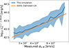 |
Fig. 6. Scaling relation between X-ray luminosity and measured velocity dispersion. The result from our simulation (the real AXES) is shown in blue (orange). We find excellent agreement between the mock and real data in Damsted et al. (2024). |
5. Selection function
In this section, we report our results about the sample completeness, directly encoded in the selection function, and purity. These results include the combination of the four light cones described in Sect. 2.1 into a single summary catalogue. We express the true X-ray flux in the 0.5–2.0 keV band within R500c.
5.1. Sample completeness
Information and knowledge about the sample completeness level is necessary to characterize the population of galaxy clusters and groups from a sample such as X-GAP. Our end-to-end mock allowed us a direct comparison between the halo population selected in the optical and X-ray bands to the global one in the full light cone. We start by analysing the fraction of selected sources as a function of X-ray flux and velocity dispersion. Just like for the luminosity, we use fluxes within R500c in the 0.5–2.0 keV band. The result is shown in Fig. 7. We see that the probability of detection is higher (in red) for bright systems with high velocity dispersion, and therefore high mass. However, we notice that the detection depends primarily on flux, rather than velocity dispersion. In the top panel of Fig. 7, at fixed velocity dispersion σv,T = 400 km/s, the detection probability changes from about 53% at X-ray flux of 2 ×10⁻¹² erg/s/cm2 to about 86% at 8 ×10⁻¹² erg/s/cm2. Conversely, it varies only from 75% at fixed flux of 5 ×10⁻¹² erg/s/cm2 for σv,T of 250 km/s to 81% at 1000 km/s. Although flux and velocity dispersion are inevitably intrinsically correlated, their impact on detection is not strongly linked. The same holds for redshift in comparison to X-ray flux. In the middle panel of Fig. 7 the detection probability is one for flux above 4 ×10⁻¹¹ erg/s/cm2 at each redshift, whereas faint sources at about 1 ×10⁻¹³ erg/s/cm2 are not detected even if they are nearby. This result is in agreement with Damsted et al. (2024), who find a small redshift evolution of the 10% completeness limit of AXES, from about 300 km/s at z = 0.05–480 km/s at z = 0.15. The bottom panel of Fig. 7 shows the detection probability as a function of redshift and velocity dispersion. In this case we do see a combined evolution. At z = 0.1, the completeness fraction increases from about 0.1% at σv,T = 300 km/s to 78% at σv,T = 1000 km/s. Similarly, at z = 0.02 it increases from 40% to 1. This trend is encoded in the correlation between more massive systems with larger velocity dispersion and X-ray brightness, meaning that the X-ray sensitivity is driving the variation of detection probability with redshift and velocity dispersion. We stress that this is true for our particular survey set up and does not necessarily hold for other selection criteria. Indeed, this is the result of the ROSAT selection being the limiting factor compared to the SDSS one. In an opposite case, with a deep X-ray coverage and a shallow optical one, the main driver of the selection method would likely be the optical proxy. Finally, we notice that the average R500c of the simulated systems in the X-GAP redshift range of 0.02–0.06 is equal to about 8 arcminutes and the average size of the detected systems is 11 arcminutes. This confirms that the size of the wavelet scales equal to 12 and 24 arcminutes in Damsted et al. (2024) is suitable to detect X-GAP groups using emission from their outskirts.
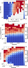 |
Fig. 7. Two-dimensional probability of detection for X-ray plus optically selected haloes in our simulation (see Sect. 5.1). The panels shows the completeness fraction as a function of three combinations of X-ray flux, velocity dispersion, and true velocity dispersion. |
5.2. Selection function model
The selection function encodes the probability for a source to be detected as a function of a given set of parameters. We compute the ratio between the detected and the simulated sources:
 (14)
(14)
In particular, we evaluate the ratio in Eq. (14) as a function of observable properties. This makes our selection function directly related to observations, bypassing intrinsic halo properties (e.g. halo mass), that are not directly measurable. When using multi wavelength data for the identification of clusters and groups, accounting for mass tracers using different observables is key to model selection effects in different surveys (e.g. Finoguenov et al. 2020). We use the X-ray flux in the 0.5–2.0 keV band within an aperture equal to R500c (computed following Sect. 3.4), velocity dispersion (see Eq. (3)), and redshift. The result is shown in Fig. 7. This combination is particularly suitable in the case where the selection function is needed for forward-modelling a population. One caveat is that one would need to account for an aperture correction since the radius encompassing an average density that is 500 times larger than the critical density depends on cosmology. It is possible to account for it by modelling its evolution with  . In the opposite case, where one wants to start from the data and does not necessarily have access to M500c, a selection function expressed in terms of flux measured within a fixed angular aperture is more convenient. Therefore, we add a second model on top of the base one, where we model the detection probability as a function of observed flux within an angular aperture of six arcminutes, velocity dispersion, and redshift. In addition, the latter model does not depend on any mass assumptions to estimate the radial aperture, which is also makes it useful for forward-modelling.
For both cases, we expect massive, bright, and nearby sources to be easier to detect compared to lighter, fainter, further ones. Therefore, the completeness is directly proportional to flux and velocity dispersion, and inversely proportional to redshift. In the previous paragraph describing Fig. 7, we notice that our selection is primarily driven by X-ray flux, which is the main variable of our model. We combine individual sigmoid functions into a comprehensive detection probability model with four free parameters, that reads:
![Mathematical equation: $$ \begin{aligned}P_{\mathrm {det}}(F_{\mathrm {X}}, z, \sigma _{\mathrm {v,T}}) =\ (1 &+ \exp [-\alpha _{\mathrm {Fx}}(\log _{\mathrm {10}}F_{\mathrm {X}} - F_{\mathrm {X,0}}) \ + \\ & - \alpha _{\mathrm {\sigma v}} \times \log _{\mathrm {10}}\sigma _{\mathrm {v,T}} + \alpha _{\mathrm {z}} \times \log _{10}z])^{-1}, \end{aligned} $$](/articles/aa/full_html/2025/07/aa53977-25/aa53977-25-eq30.gif) (15)
(15)
where the parameters αFx, αz, ασv regulate the slope of the global sigmoid function, and FX,0 sets the flux scale to centre its zero point along the flux axis. A similar approach was followed by Clerc et al. (2018), who modelled the detection of extended sources in eROSITA simulations with an error function. We find that a sigmoid allowed us to better capture the completeness trend in our simulations. To test the performance of our fit, we compute a reduced  , where F is the number of degrees of freedom, that is, the number of bins minus the number of free model parameters, D is the measured completeness, δD is its uncertainty, and M is the best-fit model evaluated at the median flux, velocity dispersion, and redshift of the full population in each 3D bin. We obtain
  , therefore we conclude that our fit is adequate. We derive posterior probability distributions and the Bayesian evidence for the parameters in Eq. (15) with the nested sampling Monte Carlo algorithm MLFriends (Buchner 2016, 2019) using the UltraNest11 package (Buchner 2021).
The result for the base model using F500c is shown in Fig. 8. The three panels show the detection probability with all combinations of flux, velocity dispersion, and redshift. The circles and squares represent the measurements from the end-to-end mocks, while the lines and shaded areas denote the best-fit model with 68% and 95% confidence intervals. The error bars account for the Poisson uncertainty in counting the total and the detected number of sources when computing the completeness (see Eq. (14)). The model favours a selection driven by flux, as noted in the previous section, with a secondary dependence on redshift and velocity dispersion. We find good agreement between the measured completeness and the model of the selection function. The full marginalised posterior distribution is shown by the green contours in Fig. 9. There is a negative correlation between the parameters describing the slope and flux normalisation, with a Pearson correlation coefficient of −0.75. This is unexpected because if the zero point is set to fainter fluxes, the slope needs to be shallower to describe the bulk of the population. However, this effect is mitigated by the positive correlation of FX,0 to the slopes related to velocity dispersion and redshift, with Pearson coefficients respectively equal to 0.98 and 0.79. We find also a positive correlation between the slopes related to redshift and velocity dispersion, with a coefficient of 0.69. This is expected by construction, because even if the detection probability increases with velocity dispersion and decreases with redshift, the sign in slope definition is opposite in Eq. (15). The results for the additional model using the flux within six arcminutes are qualitatively very similar to the base model using flux within R500c. The flux and the velocity dispersion slopes are compatible within 1σ. The flux normalisation is slightly larger at −10.84 ± 0.15 compared to −11.03 ± 0.14. One would naively expect the opposite, because at the average redshift (equal to 0.075) of our detected population, the mean R500c covers about 7 arcminutes, meaning that the integrated flux within a smaller aperture of six arcminutes should end up in a lower normalisation of the sigmoid function. However, this effect is counter balanced by the positive correlation between the flux normalisation and redshift slope, which is steeper in this second case at 2.19 ± 0.12 compared to 1.73 ± 0.12 for the base model. The larger slope values push the flux normalisation to higher values as well, but at fixed flux the completeness is higher for the model using flux within six arcminutes compared to the base one, as expected. All the parameters are reported in Table 2.
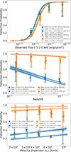 |
Fig. 8. Probability of detection for X-GAP-selected haloes as a function of observables. The three panels show different combinations of flux measured within R500c, redshift, and velocity dispersion on the x-axis in different colours and with different symbols. The various line styles denote the selection function model in Eq. (15). The error bars account for the Poisson error on the number of total and detected sources. The lines in each panel were shifted by −0.02, −0.01, 0, and 0.01 dex for clarity. |
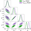 |
Fig. 9. Marginalised posterior distribution of the best-fit model of the X-ray plus optical selection function (see Eq. (15)). The filled 2D contours show the 1σ and 2σ confidence levels of the posteriors after convolution with the uniform priors. The green contours denote the base selection function where flux is measured within R500c, the violet contours show the effect of measuring flux within an angular aperture of six arcminutes. The parameter values are reported in Table 2. |
5.3. Purity-completeness trade-off
In the previous subsection, we analysed the sample completeness after cross-matching the input dark matter haloes to the X-ray and optical mocks. Instead, we did the opposite in this instance, that is, we started from the output mock catalogues and queried the matched haloes from the procedure outlined in Sect. 4. To compare the X-ray and optical catalogues we follow a prescription similar to Damsted et al. (2024). For each optical detection, we estimate R200c from a halo mass inferred from the measured galaxy velocity dispersion, based on the scaling relation calibrated in the next section. We stress the fact that this is not necessarily a precise and accurate measure of groups’ radii, but we simply use it as an aperture to search for X-ray matches. We consider an optical group to have a corresponding X-ray detection if there is a wavelet detection within the R200c estimated from velocity dispersion. This process allowed us to measure the purity of our sample, that is, the fraction of sources detected in the simulation that correspond to real input objects.
Since defining an input property for a source that is not matched to an input halo is impossible, we analyse purity as a function of a measured quantity: velocity dispersion. The result is shown in the left hand panel of Fig. 10. The blue line denotes the global population detected in the optical mock, after the application of CLEAN. The orange line considers only optical detections with a corresponding X-ray detection. The dashed black line shows the global distribution of the measured velocity dispersion in our mocks. The central panel shows the comparison to the full distribution in the real AXES sample (in pink), where the dashed lines denote the population with an X-ray match. We find that distributions in our mock and in the real AXES peak at the same velocity dispersion, and have a similar distribution, especially around the peak. This is an additional confirmation that our end-to-end simulations produce a high fidelity sample that matches the properties of the real AXES. In addition, it enables a reliable estimate of the purity level in AXES using the results from the mock. We find that the sample with an X-ray detection is very pure, reaching a purity of 90% already at σv,M = 280 km/s. The full optical mock reaches a similar purity level at about σv,M = 600 km/s. This means that the cross-correlation with X-ray practically serves as a cleaning of the optical catalogue, confirming the finding of Damsted et al. (2024). In fact, the overall distribution of measured velocity dispersion for all detections with an X-ray match peaks at higher values compared to only optical detections, with values of about 450 km/s and 350 km/s respectively. Using the full AXES population and our purity estimate from the simulation, we can estimate the purity level in the real data:
 (16)
(16)
where fobs is the fraction of real sources at a given velocity dispersion, and Psim is the purity estimate from the simulation. We estimate a purity level of 76% in the optical-only detection, and a 93% purity level in the AXES sample after adding the X-ray matching.
 |
Fig. 10. Trade-off between completeness and purity as a function of velocity dispersion. Left panel: Fraction of objects with a corresponding real input dark matter halo as a function of measured velocity dispersion. The blue line shows the fraction of objects detected in the optical mock that are matched to a real halo in the light cone. The orange line denotes objects with a corresponding X-ray detection. The green and red lines refer to the low redshift population, in the interval of interest for X-GAP, between 0.02 and 0.06. The black line shows the normalised distribution of measured velocity dispersion in the simulation. Central panel: Distribution of the measured velocity dispersion in our mock and in the real data. The blue and orange lines are left as a reference from the previous panel. The pink lines show the normalised distributions of the real AXES sample from Damsted et al. (2024), while the black ones refer to the simulation. The solid (dashed) lines denote the full optical (optical plus X-ray) detections. Right panel: Fraction of real input dark matter haloes with a corresponding detection in the mock. The coloured lines represent the same populations as the top panel, but starting from the true input dark matter haloes. |
We also study the detection performance in the lower redshift range between 0.02 and 0.06, where X-GAP is defined. The result is denoted by the green and red lines, that are the analogue of the blue and orange ones respectively, but for the low redshift population. When accounting only for the optical detection, the purity for the latter is lower than the global population by about 5–10% up to 500 km/s, where the two distributions start to agree within error bars. This is due to the fact that in the nearby Universe the SDSS galaxy sample contains a larger fraction of galaxies with low stellar mass. In the 0.02–0.06 range, the average stellar mass is about 2 × 10¹⁰ M⊙, whereas at higher redshift between 0.06–0.14, it increases to about 5 × 10¹⁰ M⊙. Therefore, the fraction of isolated galaxies at low redshift is higher, and the chance of merging them together into a fake detection is higher. However, there is excellent agreement between the orange and the red lines, meaning that after adding the X-ray match to the optical detections, the purity level is very stable for different redshift.
The effect of the X-ray correlation is also clear in the right hand panel of Fig. 10. It shows the completeness fraction as a function of true velocity dispersion, the same concept analysed in the previous section, in this case marginalised on flux and redshift. The optical catalogue reaches a 50% completeness at velocity dispersion equal to about 500 km/s, while the optical plus X-ray case requires about 730 km/s. This is due to the relatively shallow and low resolution coverage of the ROSAT all sky survey, which allowes us to detect only massive bright systems in large fractions. Conversely to purity, we see a significant improvement of the detection probability as a function of velocity dispersion at low redshift. In the 0.02–0.06 range, the 50% completeness is reached at 300 km/s. When adding the X-ray match, the same completeness level is reached at about 450 km/s. Both cases are an improvement by a factor of about 1.6 compared to the full population. The higher completeness at low redshift is also evident in the global distribution of measured velocity dispersion, the brown lines in the top panel of Fig. 10. In fact, such distribution peaks at 250 km/s and at 350 km/s when adding the X-ray match. Both are about 100 km/s lower than the peak of the distribution for the full population, even if the underlying true velocity dispersion follows a very similar trend (brown line in the bottom panel of Fig. 10): at low redshift we are able to probe the groups population down to lower velocity dispersion. We stress that this redshift trend is encoded in the selection function defined in terms of flux. We conclude that combining X-ray detected clusters and groups in the RASS with optical FoF detections provides pure samples even at low velocity dispersions, at the cost of reducing the sample completeness. However, the latter can be accounted for via the selection function calibrated in the previous section.
6. Mass – velocity dispersion
In the section, we use our mock to calibrate the scaling relation between halo mass and velocity dispersion. Within the scaling relation we account for two distributions. The first one is a log-normal distribution of the true velocity dispersion σv,T (see Eq. (3)) around the linear relation with halo mass. The second one is another log-normal distribution of the measured velocity dispersion σv,M (see Sect. 4.2) around the true one.
Following the work from Munari et al. (2013) and Ferragamo et al. (2022), we model the relation between the true velocity dispersion and halo mass using a power law model with normalisation A and slope α. In addition, we add the intrinsic scatter of the true velocity dispersion at fixed halo mass σintr. Finally, we consider the measured velocity dispersion to be distributed around the true value in a log-normal way with a scatter of σmeas. We report the two scatters σintr and σmeas in units of dex, they are the scatters of the base 10 logarithm of velocity dispersion. We also account for the measurement uncertainty of velocity dispersion on top of the scatter between measured and true velocity dispersion. This mitigates the lower precision of the velocity dispersion measurement for systems with a lower amount of members. Overall, our hierarchical formalism reads as follows:
 (17)
(17)
where θ is the collection of parameters describing the scaling relation, in our case A, α, σintr, σmeas. The normalisation A is always expressed in units of km/s. The last term P(I|σv,T,z) is the detection probability. We model it similarly to Eq. (15), but with a single sigmoid function for velocity dispersion. It depends on two parameters, the slope and normalisation, similarly to the corresponding flux terms in Eq. (15). We find a slope of 6.4 (10.8) and a normalisation of 2.64 (2.68) for the optically (optically plus X-ray) detected systems. Accounting for the detection probability allowed us to down-weight the low-mass groups that are less likely to be detected in the forward model of the selection process within the likelihood formalism. We perform five different fits in total. For the first three we focus on the true velocity dispersion. For the last two we account for the measured velocity dispersion and use the full calibration described above. In this section we focus on M200c, for consistency with the literature about velocity dispersion in clusters and groups. In Appendix B we calibrate the relation as a function of M500c, which is the mass measured for X-GAP galaxy groups (Eckert et al. 2024).
We note that when studying the scaling relation with real data, disentangling the two components of true and measured velocity dispersion is not feasible. However, this is possible within our framework, as we have access to σv,T in the simulations. This allowed us to separate the selection function, defined in terms of true observable halo properties, and the measurement of such observables, that in this case is σv,M.
6.1. True scaling relation
We first analyse the three cases focusing on the true velocity dispersion with different selections. The first case describes the full halo population in our light cone and does not account for any selection effect. The second one adds the optical selection, and the third one combines the optical selection with the X-ray one. Any discrepancy between these cases would allows us to understand the impact of selection effects on the true scaling relation.
We derive posterior probability distributions and the Bayesian evidence with the MLFriends algorithm using the UltraNest package. The full marginalised posterior distributions are shown in Fig. 12. We find a positive degeneracy between the normalisation and the slope of the scaling relation. This is expected, because the normalisation fixes the amplitude of the relation at high mass, therefore, a shallower slope is required to model the bulk of the population for a smaller normalisation. For the M200c case, the 1-D marginalised posteriors are A = 1145.1±3.9 and α = 0.330±0.001. We find a scatter for the true velocity dispersion of σintr = 0.073±0.001, confirming the tight distributions presented by Munari et al. (2013) and Ferragamo et al. (2022). The end result is shown in the top panel of Fig. 11, displaying the scaling relation between the true velocity dispersion computed using subhalo velocities (see Eq. (3)) and halo mass. The blue line denotes the best-fit model, the red lines include the intrinsic scatter σintr. Our result is compatible with the orange and green lines, referring to Munari et al. (2013) and Ferragamo et al. (2022), respectively. When adding the optical and the X-ray selections, we find a scaling relation with lower slope and normalisation. However, all three best fits are in excellent agreement within the intrinsic scatter of the scaling relation. The intrinsic scatter decreases from 0.073 for the full halo sample to 0.067 when adding the optical selection, and to 0.057 when including also the X-ray selection. This suggests that confirming the presence of a halo with one or multiple proxies gets rid of outliers, with velocity dispersions that are far from the mean scaling relation of fixed halo mass. All the parameters are reported in Table 3.
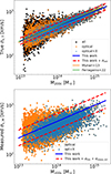 |
Fig. 11. Scaling relation between velocity dispersion and halo mass. Top panel: Scaling relation for the true velocity dispersion (Eq. (3)). The orange and green lines show the results from Munari et al. (2013) and Ferragamo et al. (2022). Bottom panel: Scaling relation for the measured velocity dispersion (Sect. 4.2). The blue line denotes the best-fit relation, and the red lines include the contribution of the intrinsic and measurement scatter summed in quadrature (see Eq. (17)). |
Priors and posteriors of the scaling relation between halo mass M200c and velocity dispersion.
6.2. Full calibration
We perform a full calibration of the velocity dispersion-halo mass relation by accounting for the distribution of the measured velocity dispersion around the true value. For the fourth and fifth case we add the measured velocity dispersion and apply the full formalism in Eq. (17). In the first place, we only study haloes detected in the optical mock, then secondly we add the X-ray selection. The bottom panel of Fig. 11 shows σv,M as a function of halo mass. In this case, the red lines include the contribution of the two scatters σintr and σmeas summed in quadrature, with the inclusion of measurement uncertainty as in Eq. (17). The posterior distribution is shown in the bottom panel of Fig. 12. The scatter for the measured velocity dispersion assumes larger values of σmeas = 0.102±0.001. The recovery of the normalisation, slope, and intrinsic scatter is in excellent agreement with the true velocity dispersion case analysed in the previous section. This is key, because it means that our formalism in Eq. (17) allowed us to recover the base scaling relation also when accounting for the measurement of velocity dispersion. The same holds for the addition of the X-ray selection on top of the optical one, with a similar measurement scatter of σmeas = 0.102±0.001. We emphasize that it is not possible to directly disentangle intrinsic and measurement scatter in observational data, as the true velocity dispersion is not accessible. However, this distinction is valuable in the context of forward-modelling, where true velocity dispersions can be generated as a function of halo mass including intrinsic scatter, and the observed values are subsequently modelled by incorporating measurement uncertainties around the true values. This approach enables a more accurate connection between observations and halo mass by appropriately accounting for both sources of scatter.
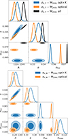 |
Fig. 12. Marginalised posterior distributions of the best-fit scaling relation parameters between velocity dispersion and M200c. The filled 2D contours show the 1-σ and 2-σ confidence levels of the posteriors after convolution with the uniform priors. The model is given by Eq. (17). The corresponding 1D parameter constraints are reported in Table 3. The top panel refers to direct relation between true velocity dispersion and halo mass, with black contours referring to the full sample, orange ones to clusters and groups detected in the optical mock, and blue ones with the addition of the X-ray detection. The bottom panel refers to the full model of the scaling relation accounting for the measured velocity dispersion. |
Finally, we test whether our assumption that the measured velocity dispersion is log-normally distributed around the true value is justified. We measure the ratio between measured and true velocity dispersion as a function of recovered number of CLEAN members. The result is shown in Fig. 13. The red line shows the gapper velocity dispersion measured by the CLEAN algorithm, the blue one denotes the estimate of the FoF finder. We do not see significant differences between them here.
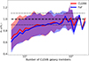 |
Fig. 13. Ratio of the measured and true velocity dispersion as a function of the number of recovered galaxy members. The red line shows the gapper velocity dispersion measured by the CLEAN algorithm, and the blue line refers to the direct estimate from the FoF finder. The dashed black line denotes the one-to-one ratio, and the dotted lines include a 10% deviation from unity. |
The ratio is systematically low for poor systems. About 20 members are required for a 10% accuracy in the measurement of velocity dispersion. We notice that this does not mean that the members have to be true group members. The misidentification of nearby galaxies that are not however gravitationally bound to the main halo from the dark matter point of view likely contributes to the scatter around the 1:1 ratio in Fig. 13. Our result is consistent with Marini et al. (2025), who find a large scatter between true halo mass and mass inferred from velocity dispersion spanning values between 25% and 40%, based on different optical finders for a GAMA-like survey. To assess whether the discrepancy between true and measured velocity dispersion for poor groups and clusters had an impact in our calibration of the total scaling relation, we tested a similar run by allowing the measured velocity dispersion to be biased compared to the true value, that is,
 (18)
(18)
where m, q describe the linear relation between the logarithmic values of measured and true velocity dispersion. On the one hand, we obtain m = 0.85±0.01 and q = 0.06±0.01, in agreement with the fact that their ratio does not follow a perfect 1:1 relation, as suggested by Fig. 13. This also means that estimating mass via velocity dispersion can be problematic also for massive galaxy clusters if the cluster is poor. This is a matter of galaxy population rather than halo mass. The majority of X-GAP groups are rich (Eckert et al. 2024), so accounting for velocity dispersion in the mass calibration is justified for large part of the sample. On the other hand, the scaling relation parameters are unbiased compared to the standard case (see Figs. 12, 11). We obtain a normalisation of 1124.3 ± 6.5, a slope of 0.335 ± 0.01, and an intrinsic scatter of 0.056 ± 0.001, all in great compatibility with the last column of Table 3. The additional uncertainties in the measurement of velocity dispersion just contributes to the measurement scatter, in fact we obtain a value of 0.078 ± 0.002 compared to 0.106 ± 0.02. We note that the linear model in Eq. (18) may not perfectly capture an effect that vanishes for rich systems. Nevertheless, given the results presented above, we expect that a more complex model would yield an even lower measurement scatter while preserving the same scaling relation parameters. We conclude that when using velocity dispersion as a mass proxy, accounting for measurement uncertainties and modelling the distribution around its true value, even with a simple lognormal function, is a key step towards retrieving an unbiased relation to halo mass.
7. Discussion and conclusions
We summarise our work and discuss the results we obtained in the previous sections further in terms of the group surface brightness and dynamical state. This final discussion aims to highlight the implications of our findings and place them in the broader context of galaxy group evolution and selection effects.
7.1. Surface brightness shape
The wavelet detection scheme is designed to detect groups and clusters using the emission from the outskirts. It is therefore not sensitive to the core properties, such as a peaked surface brightness profile in relaxed systems with an efficient cooling (Eckert et al. 2011). We therefore did not introduce a direct correlation between the dynamical state of dark matter haloes and the X-ray core properties.
We tested whether this assumption is valid by studying the detection probability as a function of the shape of the surface brightness profiles generated from the neural network in Sect. 3. We encoded the surface brightness shape in the ratio of the emissivity at R500c and in the inner most bin. When the ratio is low, the system is more similar to a cool core with a steep profile. Conversely, a high ratio means that the profile is flatter and the system is closer to a non-cool core. The result is shown in Fig. 14. The top panel shows the completeness fraction as a function of the profile ratio for different flux intervals identified by the various colours. No clear trend of the detection probability as a function of the profile ratio is visible, meaning that the detection process is not highly sensitive to the surface brightness shape. This holds from faint systems with an X-ray flux below 7 × 10⁻¹³ erg/s/cm2 where the completeness is close to zero to bright systems with a flux higher than 5 × 10⁻¹² erg/s/cm2, with a detection probability higher than 80%. In the bottom panel of Fig. 14, we split our population into cool cores and non-cool cores by selecting systems with a profile ratio that is below and above the median ratio, which is equal to 0.55. We show the completeness fraction as a function of flux for these two populations and find no significant difference between them. The two panels in Fig. 14 confirm that the wavelet detection scheme is not sensitive to the dynamical state and the core properties of clusters and groups in our simulation. Finally, it is justified to assume a constant metallicity profile because variations in metallicity would primarily affect the shape of the surface brightness profile, to which our selection method is largely insensitive.
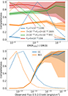 |
Fig. 14. Probability of detection as a function of core properties. The dashed lines represent the normalised distribution of the full population. Top panel: Completeness fraction as a function of emissivity profile ratio measured at R500c and in the inner most bin. Different flux intervals are encoded in different colours. Bottom panel: Completeness fraction as a function of flux for the cool core (non-cool core) systems with profile ratio smaller (larger) than the median values of 0.001. |
7.2. Dynamical state
The dynamical state of dark matter haloes hosting galaxy clusters and groups has frequently been studied in past decades in theory and simulations (Neto et al. 2007; Prada et al. 2012; Klypin et al. 2016; Seppi et al. 2021; De Luca et al. 2021) and through observations (Wojtak & Łokas 2010; Eckert et al. 2011; Ota et al. 2020; Ghirardini et al. 2022; Seppi et al. 2023; Cerini et al. 2023). From the point of view of dark matter alone, various parameters that are linked to the halo rotational properties and/or merger history were used to characterize the dynamical state of haloes. A popular choice was a combination of the spin parameter and the offset parameter. They are defined as
 (19)
(19)
where J is the halo angular momentum, E is its total energy, Rpeak is the position of the deepest point in the potential well, and RCM is its centre of mass. A disturbed or recently merged halo has a high ratio of rotational kinetic to gravitational energy and a large offset between the peak and centre-of-mass positions. Therefore, the spin and offset parameter values will both be higher than for a relaxed halo according to the definitions in Eq. (19). Following the popular thresholds for these parameters of 0.07 (see e.g. Neto et al. 2007; Klypin et al. 2016; Seppi et al. 2021), we divided our halo population detected in the optical mock into a relaxed and an unrelaxed sample. The sample selection is shown in Fig. 15. It displays the halo distribution in the spin-offset parameter plane.
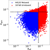 |
Fig. 15. Selection of relaxed and unrelaxed groups from the point of view of the dark matter halo ba sed on the spin and offset parameters. |
We repeat the scaling relation analysis explained in Sect. 6 to the individual samples selected from haloes matched with an optical detection. We use the same priors as the ones for the primary analysis in Table 3. The results are qualitatively similar, the posterior distributions are shown in Fig. 16. The slope of the scaling relation is compatible within 1σ for the two populations, assuming values of 0.333 ± 0.002 and 0.329 ± 0.002. However, the normalisation is significantly different, meaning that at fixed halo mass, a relaxed halo tends to host a group or cluster with higher velocity dispersion. The normalisation is 1147.1 ± 6.3 for the relaxed population, compared to 1074.0 ± 7.8 for the disturbed one. One may expect the opposite, with unrelaxed groups that are in the evolutionary stage of undergoing tidal interactions and mergers hosting a galaxy population with irregular velocities, ultimately increasing velocity dispersion at fixed mass.
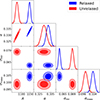 |
Fig. 16. Full marginalised posterior distribution for the scaling relation between halo mass and velocity dispersion for relaxed and unrelaxed haloes. |
To investigate this discrepancy, we measure the average distance of the recovered galaxy members from the halo centre as a function of halo mass. The result is shown in Fig. 17. In particular, the bottom panel shows the ratio of the average member distance between the disturbed and the relaxed population. It is always higher than 1 throughout the whole mass range, spanning between an increase of at least 5%, up to 10% at different masses. This means that for relaxed haloes, the member galaxies are probing a more central region of the gravitational potential compared to the disturbed case. Velocity dispersion tends to increase radially up to about the scale radius (Hoeft et al. 2004; Faltenbacher & Diemand 2006), and tends to decrease toward the outer regions. Since both radii used to describe clusters and groups, such as R200c or R500c, are significantly larger than the scale radius (depending on halo concentration, see Klypin et al. 2016), the members of relaxed groups and clusters are tracing a region of the potential with larger velocity dispersion, explaining the higher normalisation of the scaling relation measured in Fig. 16.
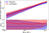 |
Fig. 17. Average galaxy member distances from the halo centre as a function of halo mass. The blue line denoted relaxed haloes, and the red line refers to disturbed ones. |
We stress that our formalism (see Eq. (17)) within the full calibration allowed us to probe the true velocity dispersion, which is unaffected by interlopers. This implies that the observed difference in normalisation is encoded in the radial distribution of member galaxies, which varies with the dynamical state of the halo. This effect plays a more significant role than the presence of galaxies with irregular velocities in disturbed systems. The latter effect rather contributes to the intrinsic scatter: the relaxed haloes trace a population with a velocity dispersion that lies closer to the mean relation to halo mass compared to the disturbed ones, in fact the intrinsic scatter is lower at 0.063 ± 0.001 compared to 0.069 ± 0.001. Because of projection, it is more likely to observe a merger closer to the 2D sky plane than along the 1D line of sight. Nonetheless, the line of sight velocity dispersion is able to capture the larger scatter in disturbed haloes. Finally, one might expect disturbed haloes to contain a higher fraction of interlopers, which would introduce additional scatter in the measured velocity dispersion. However, we find that the measured dispersions for disturbed (σmeas = 0.099 ± 0.002) and relaxed (σmeas = 0.104 ± 0.002) haloes are compatible within 1.7σ, indicating no statistically significant difference. This suggests that CLEAN is effectively removing interlopers in both relaxed and disturbed systems, ensuring robust velocity dispersion measurements.
7.3. Summary and comparison to other works
We produced and analysed a full end-to-end mock sky in the optical and X-ray wavelengths with the goal of forward-modelling the selection function of the X-GAP galaxy group sample (Eckert et al. 2024), a collection of 49 galaxy groups that were selected by cross-matching extended sources in the Rosat All Sky Survey (RASS) and FoF galaxy groups and clusters in the SDSS area (Tempel et al. 2017; Damsted et al. 2024). The workflow was summarised in Fig. 1. We built a dark matter halo light cone using individual snapshots of the Uchuu simulation (Ishiyama et al. 2021) (see Fig. 2) and adapted dedicated simulations of the SDSS sky (Dong-Páez et al. 2024). We developed a novel method for populating dark matter haloes with X-ray emission using an optimised neural network informed by hydrodynamical simulations to simulate emissivity profiles and temperatures with the proper covariances in terms of mass and redshift. We demonstrated that our model is able to predict the observed distributions of cluster and group profiles and observables and recovers scaling relations with halo mass for the X-ray luminosity and temperature with observations (see Sect. 3, Fig. 3 and 4). We used the AGN model from Comparat et al. (2019) and generated a mock X-ray diffuse background by resampling the real RASS background maps. We generated X-ray photons using SIXTE (Dauser et al. 2019), and we accounted for the instrumental response and observing strategy of the spacecraft.
We ran a wavelet-based detection scheme (Vikhlinin et al. 1998; Käfer et al. 2019) on the mock X-ray images and a FoF finder on the mock galaxies to obtain galaxy group candidates. We cross-matched the output catalogues with the dark matter halo light cone using the information stored in the source ID generating each X-ray event and the parent IDs stored for each galaxy member of the optical groups. An example for a field of one square degree that covers a massive cluster in the mock is shown in Fig. 5.
We measured the detection probability by comparing the histogram of detected haloes to the complete population as a function of flux, velocity dispersion, and redshift. The result is shown in Fig. 7. In total, we simulated 62 868 clusters and groups at z<0.14. The global completeness is 6.3%, with the X-ray mock being the limiting factor. The completeness is 8.8%, compared to 28.1% for the optical FoF catalogue alone. We found that the detection probability mainly depends on flux and weakly depends on the velocity dispersion and redshift. This confirms that the X-GAP selection is mainly limited by the X-ray flux because the coverage of the RASS is relatively shallow. We found a 50% detection probability at about 1.5 × 10⁻¹² erg/s/cm2. This 50% flux limit is about five times higher than the estimate for the first eROSITA all sky survey (eRASS1) that carried out by Seppi et al. (2022), at about 3 × 10⁻¹³ erg/s/cm2. Since the average exposure time is comparable between eRASS1 and the X-GAP area covered by the RASS, the difference resides in the higher eROSITA sensitivity compared to ROSAT based on its efficient grasp, that is, the effective collecting area multiplied by the field of view, which is larger than the ROSAT field of view by about three at 1 keV. Previous work by Clerc et al. (2018) estimated an average 50% completeness at 6 × 10⁻¹⁵ erg/s/cm2 for the cumulative sum of eight eROSITA all sky surveys. In this case, the much lower flux limit is also due to the increment in exposure time, which reaches average values of more than 1.5 ks compared to our average coverage of about 400 s. Pointed programs such as the XMM-XXL survey (Pierre et al. 2016), which covers about 50 square degrees with an exposure time of about 10 ks, allow us to reach faint fluxes of 2 × 10⁻¹⁴ erg/s/cm2 at z = 0.2 (Pacaud et al. 2006), with an effective area that is comparable to that of eROSITA. The different flux limits also depend on the set-up of a detection algorithm and source classification, which makes them dependent on the scientific goal of specific project.
Various approaches have been adopted in the literature to model the selection function, from empirical methods (Bocquet et al. 2019) and analytical models (Clerc et al. 2018; Ider Chitham et al. 2020) to more complex interpolation schemes (Clerc et al. 2024). The latter is preferable when the selection is to be modelled in a very large parameter space, in which case the effort becomes computationally very expensive. For example, Clerc et al. (2024) combined 100 different realisations of a single mock to model the eRASS1 cluster detection probability and accounted for the very large variations in the exposure time and local background across the eROSITA sky in addition to the count rate, redshift, and various combinations of morphological parameters. In comparison, the X-GAP area is covered with a stable background and more uniform exposure due to the marginal overlap between the deep region around the ecliptic pole and the SDSS area. We modelled the selection function with a sigmoid distribution that accounted for a main flux component, and secondary slopes described the redshift and velocity dispersion trends. We provided two models for the selection function, one model based on the observed flux within R500c, which is ideal for forward-modelling population studies, and a second model that used flux within a fixed angular aperture of 6 arcminutes, which is useful for studies that start from the perspective of the observations. Both models captured the smooth increment of the detection probability as a function of flux and its secondary trend with increasing velocity dispersion and decreasing redshift (see Fig. 8). The expression for our model is given in Eq. (15), the best-fit parameters are reported in Table 2, and their posterior distribution is shown in Fig. 9.
We analysed the purity of the selection method by comparing the fraction of detections that is not matched to an input halo. We studied this fraction as a function of velocity dispersion in Fig. 10. We found that the X-ray data serve as a cleaning of the optical catalogue, which reaches a purity of 90% at about 280 km/s, compared to 600 km/s for the optical FoF group catalogue. A similar comparison was performed by Marini et al. (2025) and Popesso et al. (2024). Together with the FoF algorithm from Tempel et al. (2017), they tested the optical finders from Yang et al. (2005) and Robotham et al. (2011). They studied completeness and purity as a function of halo mass instead of velocity dispersion, but our calibration of the mass-to-velocity dispersion scaling relation allowed us to compare our results with their work. At M200c = 2×10¹³ M⊙, they reported a contamination level of about 6% and 15% depending on the optical finder. Although the scatter is larger at low masses, at a corresponding velocity dispersion of about 250 km/s, we obtained a higher contamination of about 35%. The discrepancy is reduced after the X-ray cleaning, where our purity increases to about 85%. Multiple effects contribute to this difference. Marini et al. (2025) focused on a GAMA-like spectroscopic survey instead of SDSS, which allowed them to reach fainter magnitudes down to 19.8 (Popesso et al. 2024). Their mock extended to z = 0.2, which means that they probed fainter magnitudes than we did, but not necessarily a galaxy population with a lower stellar mass. This is consistent with our result in Fig. 10, where the purity decreases at low redshift. In addition, our matching procedure is different because we directly involved the velocity dispersion in the matching (see Sect. 4). One additional difference is that we did not include X-ray binaries (XRB) in our mock, which lack baryons in the first place. Popesso et al. (2024) showed that the XRB contribution to the total X-ray emission is 5% at most for small groups around 1013 M⊙, and it drastically drops towards the cluster scale. A similar result using observations was reported by Anderson et al. (2015), with an X-ray luminosity from XRBs around 1040 erg/s at stellar mass M★ = 2×10¹¹ M⊙, while the total luminosity was closer to 1040 erg/s. According to Tinker (2021), this range corresponds to an halo mass of about 8 ×10¹² M⊙. We therefore consider this a negligible limitation for the purpose of this work. Nonetheless, accounting for XRBs will be relevant in the future model comparison of thermodynamical profiles to X-GAP. Finally and most importantly, the selection of the parent optical catalogue is different because they even included galaxy pairs, while we focused on groups with at least five members.
The latter point also boosted the completeness, as reported by Popesso et al. (2024), which reached levels higher than 80% in the group regime, compared to our result, where the completeness is about 20% at a velocity dispersion of about 300 km/s. This is expected because the majority of these groups are detected with a low number of members, which are naturally filtered out by our selection of at least five members. Finally, the construction of the optical simulation also plays a role. On the one hand, we used the abundance-matching prescription from Dong-Páez et al. (2024), which recovers the SDSS optical properties by construction. On the other hand, Marini et al. (2025) built an optical mock with a stellar mass function that was skewed towards massive centrals, and they tested their analysis with a different simulation that was built using the UniverseMachine software (Behroozi et al. 2019). They showed that their completeness was reduced to about 60% for galaxy groups, which reduces the difference with our work. The estimation of the completeness and purity levels using simulations is strongly sensitive to the specific survey set-up and to the assumptions made in the detection scheme. A careful modelling of the whole process is the key to properly assessing the systematics for different works.
Finally, we calibrated the scaling relation between halo mass and velocity dispersion. We accounted for two different types of scatter. The first type was the intrinsic scatter, and the second scatter was due to the uncertainty in the measurement of velocity dispersion. The scaling relation is shown in Fig. 11 and the posterior distribution of the best-fit parameters is shown in Fig. 12. Our results agree with previous work on simulations (Munari et al. 2013; Ferragamo et al. 2022). The scatter is dominated by the measurement uncertainty, assuming values of 0.102 and 0.106 for groups detected in the optical mock and with the addition of the cross-correlation to X-ray. These are about 60% larger than the respective intrinsic scatters of 0.067 and 0.057. Moreover, the measurement of velocity dispersion is accurate compared to its true value only for rich systems, with a bias lower than 10% for systems with at least 20 members (see Fig. 13). For smaller groups, the velocity dispersion is biased towards lower values. This is true also for more massive systems when they are poor. Our result agrees with that of Marini et al. (2025), who obtained halo masses inferred from a velocity dispersion that were biased low compared to the true mass from groups to clusters using the FoF finder from Tempel et al. (2017). In general, it is essential to account for the distribution of the measured velocity dispersion around its true value to recover an unbiased scaling relation to the halo mass. In the context of forward-modelling, this is usually done for mass proxies, especially in cluster count cosmological studies in the X-ray or millimeter bands using the X-ray count rate (Ghirardini et al. 2024) or Y-SZ (Bocquet et al. 2025).
The mocks and the selection function developed in this article will be used a benchmark to compare the real X-GAP data to hydrodynamical simulations in future work.
Acknowledgments
The authors thank the anonymous referee for their helpful comments that improved the quality of the article. RS and DE are supported by Swiss National Science Foundation project grant #200021_212576. RS thanks S. Krippendorf and W. Hartley for useful discussions about neural networks for this project. RS thanks F. Prada for discussions about the Uchuu simulations. ET acknowledges funding from the HTM (grant TK202), ETAg (grant PRG1006) and the EU Horizon Europe (EXCOSM, grant No. 101159513). KK acknowledges support from the South African Radio Astronomy Observatory (SARAO; www.sarao.ac.za). MAB acknowledges support from a UKRI Stephen Hawking Fellowship (EP/X04257X/1). We thank Instituto de Astrofisica de Andalucia (IAA-CSIC), Centro de Supercomputacion de Galicia (CESGA) and the Spanish academic and research network (RedIRIS) in Spain for hosting Uchuu DR1, DR2 and DR3 in the Skies and Universes site for cosmological simulations. The Uchuu simulations were carried out on Aterui II supercomputer at Center for Computational Astrophysics, CfCA, of National Astronomical Observatory of Japan, and the K computer at the RIKEN Advanced Institute for Computational Science. The Uchuu Data Releases efforts have made use of the skun@IAA_RedIRIS and skun6@IAA computer facilities managed by the IAA-CSIC in Spain (MICINN EU-Feder grant EQC2018-004366-P).
ROentgen SATellite.
Extended ROentgen Survey with an Imaging Telescope Array.
R500c is the radius encompassing an average density that is 500 times larger than the critical density of the Universe at the group redshift, ρc = 3H(z)/8πG.
References
- Abadi, M., Agarwal, A., Barham, P., et al. 2015, TensorFlow: Large-Scale Machine Learning on Heterogeneous Systems, software available from tensorflow.org [Google Scholar]
- Abell, G. O. 1958, ApJS, 3, 211 [NASA ADS] [CrossRef] [Google Scholar]
- Adami, C., Giles, P., Koulouridis, E., et al. 2018, A&A, 620, A5 [NASA ADS] [CrossRef] [EDP Sciences] [Google Scholar]
- Aird, J., Coil, A. L., Georgakakis, A., et al. 2015, MNRAS, 451, 1892 [Google Scholar]
- Anderson, S. F., Margon, B., Voges, W., et al. 2007, AJ, 133, 313 [NASA ADS] [CrossRef] [Google Scholar]
- Anderson, M. E., Gaspari, M., White, S. D. M., Wang, W., & Dai, X. 2015, MNRAS, 449, 3806 [NASA ADS] [CrossRef] [Google Scholar]
- Arnaud, K. A. 1996, in Astronomical Data Analysis Software and Systems V, eds. G. H. Jacoby, & J. Barnes, ASP Conf. Ser., 101, 17 [NASA ADS] [Google Scholar]
- Arnaud, M., Aghanim, N., & Neumann, D. M. 2002, A&A, 389, 1 [NASA ADS] [CrossRef] [EDP Sciences] [Google Scholar]
- Artis, E., Ghirardini, V., Bulbul, E., et al. 2024, A&A, 691, A301 [NASA ADS] [CrossRef] [EDP Sciences] [Google Scholar]
- Asplund, M., Grevesse, N., Sauval, A. J., & Scott, P. 2009, ARA&A, 47, 481 [NASA ADS] [CrossRef] [Google Scholar]
- Astropy Collaboration (Robitaille, T. P., et al.) 2013, A&A, 558, A33 [NASA ADS] [CrossRef] [EDP Sciences] [Google Scholar]
- Bahar, Y. E., Bulbul, E., Clerc, N., et al. 2022, A&A, 661, A7 [NASA ADS] [CrossRef] [EDP Sciences] [Google Scholar]
- Bahar, Y. E., Bulbul, E., Ghirardini, V., et al. 2024, A&A, 691, A188 [NASA ADS] [CrossRef] [EDP Sciences] [Google Scholar]
- Bartalucci, I., Molendi, S., Rasia, E., et al. 2023, A&A, 674, A179 [NASA ADS] [CrossRef] [EDP Sciences] [Google Scholar]
- Beers, T. C., Flynn, K., & Gebhardt, K. 1990, AJ, 100, 32 [Google Scholar]
- Behroozi, P., Wechsler, R., & Wu, H. -Y. 2013, ApJ, 762, 109 [NASA ADS] [CrossRef] [Google Scholar]
- Behroozi, P., Wechsler, R. H., Hearin, A. P., & Conroy, C. 2019, MNRAS, 488, 3143 [NASA ADS] [CrossRef] [Google Scholar]
- Benyas, M., Pfeifer, J., Mantz, A. B., Allen, S. W., & Darragh-Ford, E. 2024, ApJ, 969, 58 [NASA ADS] [CrossRef] [Google Scholar]
- Bertin, E., & Arnouts, S. 1996, A&AS, 117, 393 [NASA ADS] [CrossRef] [EDP Sciences] [Google Scholar]
- Biffi, V., Dolag, K., Böhringer, H., & Lemson, G. 2012, MNRAS, 420, 3545 [NASA ADS] [Google Scholar]
- Biffi, V., Dolag, K., & Böhringer, H. 2013, MNRAS, 428, 1395 [Google Scholar]
- Bîrzan, L., McNamara, B. R., Nulsen, P. E. J., Carilli, C. L., & Wise, M. W. 2008, ApJ, 686, 859 [Google Scholar]
- Blanton, M. R., Bershady, M. A., Abolfathi, B., et al. 2017, AJ, 154, 28 [Google Scholar]
- Bocquet, S., Dietrich, J. P., Schrabback, T., et al. 2019, ApJ, 878, 55 [Google Scholar]
- Bocquet, S., Grandis, S., Krause, E., et al. 2025, Phys. Rev. D, 111, 063533 [Google Scholar]
- Boese, F. G. 2000, A&AS, 141, 507 [NASA ADS] [CrossRef] [EDP Sciences] [Google Scholar]
- Böhringer, H., Voges, W., Huchra, J. P., et al. 2000, ApJS, 129, 435 [Google Scholar]
- Boissay, R., Ricci, C., & Paltani, S. 2016, A&A, 588, A70 [NASA ADS] [CrossRef] [EDP Sciences] [Google Scholar]
- Boller, T., Freyberg, M. J., Trümper, J., et al. 2016, A&A, 588, A103 [NASA ADS] [CrossRef] [EDP Sciences] [Google Scholar]
- Booth, C. M., & Schaye, J. 2009, MNRAS, 398, 53 [Google Scholar]
- Bourne, M. A., & Yang, H. -Y. K. 2023, Galaxies, 11, 73 [NASA ADS] [CrossRef] [Google Scholar]
- Buchner, J. 2016, Stat. Comput., 26, 383 [Google Scholar]
- Buchner, J. 2019, PASP, 131, 108005 [Google Scholar]
- Buchner, J. 2021, J. Open Source Softw., 6, 3001 [CrossRef] [Google Scholar]
- Bulbul, E., Chiu, I. N., Mohr, J. J., et al. 2019, ApJ, 871, 50 [Google Scholar]
- Bulbul, E., Liu, A., Kluge, M., et al. 2024, A&A, 685, A106 [NASA ADS] [CrossRef] [EDP Sciences] [Google Scholar]
- Cerini, G., Cappelluti, N., & Natarajan, P. 2023, ApJ, 945, 152 [Google Scholar]
- Chiu, I. N., Ghirardini, V., Liu, A., et al. 2022, A&A, 661, A11 [NASA ADS] [CrossRef] [EDP Sciences] [Google Scholar]
- Clerc, N., Ramos-Ceja, M. E., Ridl, J., et al. 2018, A&A, 617, A92 [NASA ADS] [CrossRef] [EDP Sciences] [Google Scholar]
- Clerc, N., Comparat, J., Seppi, R., et al. 2024, A&A, 687, A238 [NASA ADS] [CrossRef] [EDP Sciences] [Google Scholar]
- Comparat, J., Merloni, A., Salvato, M., et al. 2019, MNRAS, 487, 2005 [Google Scholar]
- Comparat, J., Eckert, D., Finoguenov, A., et al. 2020, Open J. Astrophys., 3, 13 [Google Scholar]
- Crenshaw, J. F., Kalmbach, J. B., Gagliano, A., et al. 2024, AJ, 168, 80 [NASA ADS] [CrossRef] [Google Scholar]
- Damsted, S., Finoguenov, A., Lietzen, H., et al. 2024, A&A, 690, A52 [NASA ADS] [CrossRef] [EDP Sciences] [Google Scholar]
- Dauser, T., Falkner, S., Lorenz, M., et al. 2019, A&A, 630, A66 [NASA ADS] [CrossRef] [EDP Sciences] [Google Scholar]
- Davé, R., Anglés-Alcázar, D., Narayanan, D., et al. 2019, MNRAS, 486, 2827 [Google Scholar]
- De Luca, F., De Petris, M., Yepes, G., et al. 2021, MNRAS, 504, 5383 [NASA ADS] [CrossRef] [Google Scholar]
- Dolag, K., Komatsu, E., & Sunyaev, R. 2016, MNRAS, 463, 1797 [Google Scholar]
- Dong-Páez, C. A., Smith, A., Szewciw, A. O., et al. 2024, MNRAS, 528, 7236 [CrossRef] [Google Scholar]
- Dubois, Y., Peirani, S., Pichon, C., et al. 2016, MNRAS, 463, 3948 [Google Scholar]
- Ebeling, H., Edge, A. C., & Henry, J. P. 2001, ApJ, 553, 668 [Google Scholar]
- Eckert, D., Molendi, S., & Paltani, S. 2011, A&A, 526, A79 [NASA ADS] [CrossRef] [EDP Sciences] [Google Scholar]
- Eckert, D., Vazza, F., Ettori, S., et al. 2012, A&A, 541, A57 [NASA ADS] [CrossRef] [EDP Sciences] [Google Scholar]
- Eckert, D., Ettori, S., Coupon, J., et al. 2016, A&A, 592, A12 [NASA ADS] [CrossRef] [EDP Sciences] [Google Scholar]
- Eckert, D., Gaspari, M., Gastaldello, F., Le Brun, A. M. C., & O’Sullivan, E. 2021, Universe, 7, 142 [NASA ADS] [CrossRef] [Google Scholar]
- Eckert, D., Gastaldello, F., O’Sullivan, E., et al. 2024, Galaxies, 12, 24 [NASA ADS] [CrossRef] [Google Scholar]
- Egger, R. J., & Aschenbach, B. 1995, A&A, 294, L25 [NASA ADS] [Google Scholar]
- Fabian, A. C. 2012, ARA&A, 50, 455 [Google Scholar]
- Fakhouri, O., Ma, C. -P., & Boylan-Kolchin, M. 2010, MNRAS, 406, 2267 [CrossRef] [Google Scholar]
- Faltenbacher, A., & Diemand, J. 2006, MNRAS, 369, 1698 [Google Scholar]
- Ferragamo, A., De Petris, M., Yepes, G., et al. 2022, in mm Universe @ NIKA2 – Observing the mm Universe with the NIKA2 Camera, EPJ Web Conf., 257, 00018 [NASA ADS] [CrossRef] [EDP Sciences] [Google Scholar]
- Finoguenov, A., Jones, C., Böhringer, H., & Ponman, T. J. 2002, ApJ, 578, 74 [NASA ADS] [CrossRef] [Google Scholar]
- Finoguenov, A., Rykoff, E., Clerc, N., et al. 2020, A&A, 638, A114 [NASA ADS] [CrossRef] [EDP Sciences] [Google Scholar]
- Foster, A. R., & Heuer, K. 2020, Atoms, 8, 49 [NASA ADS] [CrossRef] [Google Scholar]
- Garcia, A. M. 1993, A&AS, 100, 47 [NASA ADS] [Google Scholar]
- Gastaldello, F., Buote, D. A., Temi, P., et al. 2009, ApJ, 693, 43 [NASA ADS] [CrossRef] [Google Scholar]
- Gastaldello, F., Simionescu, A., Mernier, F., et al. 2021, Universe, 7, 208 [NASA ADS] [CrossRef] [Google Scholar]
- Geller, M. J., & Huchra, J. P. 1983, ApJS, 52, 61 [NASA ADS] [CrossRef] [Google Scholar]
- Georgakakis, A., Aird, J., Schulze, A., et al. 2017, MNRAS, 471, 1976 [NASA ADS] [CrossRef] [Google Scholar]
- Georgakakis, A., Comparat, J., Merloni, A., et al. 2019, MNRAS, 487, 275 [NASA ADS] [CrossRef] [Google Scholar]
- Germain, M., Gregor, K., Murray, I., & Larochelle, H. 2015, ArXiv e-prints [arXiv:1502.03509] [Google Scholar]
- Ghirardini, V., Eckert, D., Ettori, S., et al. 2019, A&A, 621, A41 [NASA ADS] [CrossRef] [EDP Sciences] [Google Scholar]
- Ghirardini, V., Bahar, Y. E., Bulbul, E., et al. 2022, A&A, 661, A12 [NASA ADS] [CrossRef] [EDP Sciences] [Google Scholar]
- Ghirardini, V., Bulbul, E., Artis, E., et al. 2024, A&A, 689, A298 [NASA ADS] [CrossRef] [EDP Sciences] [Google Scholar]
- Gitti, M., Brighenti, F., & McNamara, B. R. 2012, Adv. Astron., 2012, 950641 [CrossRef] [Google Scholar]
- Gladders, M. D., & Yee, H. K. C. 2000, AJ, 120, 2148 [NASA ADS] [CrossRef] [Google Scholar]
- Goodfellow, I. J., Pouget-Abadie, J., Mirza, M., et al. 2014, ArXiv e-prints [arXiv:1406.2661] [Google Scholar]
- Gozaliasl, G., Finoguenov, A., Khosroshahi, H. G., et al. 2014, A&A, 566, A140 [NASA ADS] [CrossRef] [EDP Sciences] [Google Scholar]
- Gozaliasl, G., Finoguenov, A., Tanaka, M., et al. 2019, MNRAS, 483, 3545 [Google Scholar]
- Gozaliasl, G., Finoguenov, A., Khosroshahi, H. G., et al. 2020, A&A, 635, A36 [EDP Sciences] [Google Scholar]
- Green, G. M., Ting, Y. -S., & Kamdar, H. 2023, ApJ, 942, 26 [Google Scholar]
- Hahn, C., & Melchior, P. 2022, ApJ, 938, 11 [NASA ADS] [CrossRef] [Google Scholar]
- Henden, N. A., Puchwein, E., Shen, S., & Sijacki, D. 2018, MNRAS, 479, 5385 [CrossRef] [Google Scholar]
- HI4PI Collaboration (Ben Bekhti, N., et al.) 2016, A&A, 594, A116 [NASA ADS] [CrossRef] [EDP Sciences] [Google Scholar]
- Hlavacek-Larrondo, J., Li, Y., & Churazov, E. 2022, in Handbook of X-ray and Gamma-ray Astrophysics, eds. C. Bambi, & A. Sangangelo, 5 [Google Scholar]
- Hoeft, M., Mücket, J. P., & Gottlöber, S. 2004, ApJ, 602, 162 [Google Scholar]
- Huchra, J. P., & Geller, M. J. 1982, ApJ, 257, 423 [NASA ADS] [CrossRef] [Google Scholar]
- Ider Chitham, J., Comparat, J., Finoguenov, A., et al. 2020, MNRAS, 499, 4768 [NASA ADS] [CrossRef] [Google Scholar]
- Ishiyama, T., Prada, F., Klypin, A. A., et al. 2021, MNRAS, 506, 4210 [NASA ADS] [CrossRef] [Google Scholar]
- Johnson, R., Ponman, T. J., & Finoguenov, A. 2009, MNRAS, 395, 1287 [CrossRef] [Google Scholar]
- Käfer, F., Finoguenov, A., Eckert, D., et al. 2019, A&A, 628, A43 [Google Scholar]
- Kauffmann, G., & Haehnelt, M. 2000, MNRAS, 311, 576 [Google Scholar]
- Khalil, H., Finoguenov, A., Tempel, E., & Mamon, G. A. 2024, A&A, 690, A212 [NASA ADS] [CrossRef] [EDP Sciences] [Google Scholar]
- Kingma, D. P., & Welling, M. 2013, ArXiv e-prints [arXiv:1312.6114] [Google Scholar]
- Kluge, M., Comparat, J., Liu, A., et al. 2024, A&A, 688, A210 [NASA ADS] [CrossRef] [EDP Sciences] [Google Scholar]
- Klypin, A., Yepes, G., Gottlöber, S., Prada, F., & Heß, S. 2016, MNRAS, 457, 4340 [Google Scholar]
- Knebe, A., Knollmann, S. R., Muldrew, S. I., et al. 2011, MNRAS, 415, 2293 [Google Scholar]
- Knebe, A., Pearce, F. R., Lux, H., et al. 2013, MNRAS, 435, 1618 [NASA ADS] [CrossRef] [Google Scholar]
- Kobyzev, I., Prince, S. J. D., & Brubaker, M. A. 2019, ArXiv e-prints [arXiv:1908.09257] [Google Scholar]
- Kolokythas, K., O’Sullivan, E., Raychaudhury, S., et al. 2018, MNRAS, 481, 1550 [NASA ADS] [Google Scholar]
- Kolokythas, K., O’Sullivan, E., Intema, H., et al. 2019, MNRAS, 489, 2488 [CrossRef] [Google Scholar]
- Kormendy, J., & Ho, L. C. 2013, ARA&A, 51, 511 [Google Scholar]
- Krippendorf, S., Baron Perez, N., Bulbul, E., et al. 2024, A&A, 682, A132 [NASA ADS] [CrossRef] [EDP Sciences] [Google Scholar]
- Lambert, T. S., Kraan-Korteweg, R. C., Jarrett, T. H., & Macri, L. M. 2020, MNRAS, 497, 2954 [Google Scholar]
- Le Brun, A. M. C., McCarthy, I. G., Schaye, J., & Ponman, T. J. 2014, MNRAS, 441, 1270 [NASA ADS] [CrossRef] [Google Scholar]
- Li, J., Melchior, P., Hahn, C., & Huang, S. 2024, AJ, 167, 16 [Google Scholar]
- Licitra, R., Mei, S., Raichoor, A., Erben, T., & Hildebrandt, H. 2016, MNRAS, 455, 3020 [NASA ADS] [CrossRef] [Google Scholar]
- Liu, W., Sun, M., Nulsen, P., et al. 2019, MNRAS, 484, 3376 [NASA ADS] [CrossRef] [Google Scholar]
- Liu, A., Bulbul, E., Ghirardini, V., et al. 2022a, A&A, 661, A2 [NASA ADS] [CrossRef] [EDP Sciences] [Google Scholar]
- Liu, T., Merloni, A., Comparat, J., et al. 2022b, A&A, 661, A27 [NASA ADS] [CrossRef] [EDP Sciences] [Google Scholar]
- Lovisari, L., Reiprich, T. H., & Schellenberger, G. 2015, A&A, 573, A118 [NASA ADS] [CrossRef] [EDP Sciences] [Google Scholar]
- Lovisari, L., Schellenberger, G., Sereno, M., et al. 2020, ApJ, 892, 102 [Google Scholar]
- Lovisari, L., Ettori, S., Gaspari, M., & Giles, P. A. 2021, Universe, 7, 139 [NASA ADS] [CrossRef] [Google Scholar]
- Magorrian, J., Tremaine, S., Richstone, D., et al. 1998, AJ, 115, 2285 [Google Scholar]
- Mamon, G. A., Biviano, A., & Murante, G. 2010, A&A, 520, A30 [NASA ADS] [CrossRef] [EDP Sciences] [Google Scholar]
- Mamon, G. A., Biviano, A., & Boué, G. 2013, MNRAS, 429, 3079 [Google Scholar]
- Mantz, A. B., Allen, S. W., Morris, R. G., et al. 2016, MNRAS, 463, 3582 [NASA ADS] [CrossRef] [Google Scholar]
- Marini, I., Popesso, P., Lamer, G., et al. 2024, A&A, 689, A7 [NASA ADS] [CrossRef] [EDP Sciences] [Google Scholar]
- Marini, I., Popesso, P., Dolag, K., et al. 2025, A&A, 694, A207 [NASA ADS] [CrossRef] [EDP Sciences] [Google Scholar]
- Mazzotta, P., Rasia, E., Moscardini, L., & Tormen, G. 2004, MNRAS, 354, 10 [NASA ADS] [CrossRef] [Google Scholar]
- McCarthy, I. G., Schaye, J., Bird, S., & Le Brun, A. M. C. 2017, MNRAS, 465, 2936 [Google Scholar]
- McNamara, B. R., & Nulsen, P. E. J. 2007, ARA&A, 45, 117 [NASA ADS] [CrossRef] [Google Scholar]
- Merloni, A., Predehl, P., Becker, W., et al. 2012, ArXiv e-prints [arXiv:1209.3114] [Google Scholar]
- Mernier, F., de Plaa, J., Kaastra, J. S., et al. 2017, A&A, 603, A80 [NASA ADS] [CrossRef] [EDP Sciences] [Google Scholar]
- Mo, H. J., & White, S. D. M. 2002, MNRAS, 336, 112 [Google Scholar]
- Moster, B. P., Naab, T., & White, S. D. M. 2013, MNRAS, 428, 3121 [Google Scholar]
- Munari, E., Biviano, A., Borgani, S., Murante, G., & Fabjan, D. 2013, MNRAS, 430, 2638 [Google Scholar]
- Muñoz-Cuartas, J. C., & Müller, V. 2012, MNRAS, 423, 1583 [CrossRef] [Google Scholar]
- Nandra, K., O’Neill, P. M., George, I. M., & Reeves, J. N. 2007, MNRAS, 382, 194 [NASA ADS] [CrossRef] [Google Scholar]
- Navarro, J. F., Frenk, C. S., & White, S. D. M. 1996, ApJ, 462, 563 [Google Scholar]
- Nelson, D., Springel, V., Pillepich, A., et al. 2019, Comput. Astrophys. Cosmol., 6, 2 [Google Scholar]
- Neto, A. F., Gao, L., Bett, P., et al. 2007, MNRAS, 381, 1450 [NASA ADS] [CrossRef] [Google Scholar]
- Neumann, D. M., & Arnaud, M. 1999, A&A, 348, 711 [NASA ADS] [Google Scholar]
- Ntampaka, M., ZuHone, J., Eisenstein, D., et al. 2019, ApJ, 876, 82 [NASA ADS] [CrossRef] [Google Scholar]
- Old, L., Skibba, R. A., Pearce, F. R., et al. 2014, MNRAS, 441, 1513 [Google Scholar]
- Old, L., Wojtak, R., Mamon, G. A., et al. 2015, MNRAS, 449, 1897 [Google Scholar]
- Onions, J., Knebe, A., Pearce, F. R., et al. 2012, MNRAS, 423, 1200 [Google Scholar]
- Oppenheimer, B. D., Babul, A., Bahé, Y., Butsky, I. S., & McCarthy, I. G. 2021, Universe, 7, 209 [NASA ADS] [CrossRef] [Google Scholar]
- Osato, K., & Nagai, D. 2023, MNRAS, 519, 2069 [Google Scholar]
- O’Sullivan, E., Ponman, T. J., Kolokythas, K., et al. 2017, MNRAS, 472, 1482 [CrossRef] [Google Scholar]
- O’Sullivan, E., Combes, F., Salomé, P., et al. 2018, A&A, 618, A126 [NASA ADS] [CrossRef] [EDP Sciences] [Google Scholar]
- Ota, N., Mitsuishi, I., Babazaki, Y., et al. 2020, PASJ, 72, 1 [NASA ADS] [CrossRef] [Google Scholar]
- Pacaud, F., Pierre, M., Refregier, A., et al. 2006, MNRAS, 372, 578 [NASA ADS] [CrossRef] [Google Scholar]
- Pacaud, F., Pierre, M., Melin, J. B., et al. 2018, A&A, 620, A10 [NASA ADS] [CrossRef] [EDP Sciences] [Google Scholar]
- Padovani, P., Alexander, D. M., Assef, R. J., et al. 2017, A&ARv, 25, 2 [Google Scholar]
- Papamakarios, G., Nalisnick, E., Jimenez Rezende, D., Mohamed, S., & Lakshminarayanan, B. 2019, ArXiv e-prints [arXiv:1912.02762] [Google Scholar]
- Pfeffermann, E., Briel, U. G., Hippmann, H., et al. 1986, SPIE Conf. Ser., 733, 519 [Google Scholar]
- Pierre, M., Pacaud, F., Adami, C., et al. 2016, A&A, 592, A1 [NASA ADS] [CrossRef] [EDP Sciences] [Google Scholar]
- Pillepich, A., Springel, V., Nelson, D., et al. 2018, MNRAS, 473, 4077 [Google Scholar]
- Planck Collaboration VI. 2020, A&A, 641, A6 [NASA ADS] [CrossRef] [EDP Sciences] [Google Scholar]
- Ponman, T. J., Cannon, D. B., & Navarro, J. F. 1999, Nature, 397, 135 [CrossRef] [Google Scholar]
- Ponman, T. J., Sanderson, A. J. R., & Finoguenov, A. 2003, MNRAS, 343, 331 [NASA ADS] [CrossRef] [Google Scholar]
- Popesso, P., Marini, I., Dolag, K., et al. 2024, A&A, submitted [arXiv:2411.16546] [Google Scholar]
- Prada, F., Klypin, A. A., Cuesta, A. J., Betancort-Rijo, J. E., & Primack, J. 2012, MNRAS, 423, 3018 [NASA ADS] [CrossRef] [Google Scholar]
- Pratt, G. W., Croston, J. H., Arnaud, M., & Böhringer, H. 2009, A&A, 498, 361 [NASA ADS] [CrossRef] [EDP Sciences] [Google Scholar]
- Predehl, P., Sunyaev, R. A., Becker, W., et al. 2020, Nature, 588, 227 [CrossRef] [Google Scholar]
- Predehl, P., Andritschke, R., Arefiev, V., et al. 2021, A&A, 647, A1 [EDP Sciences] [Google Scholar]
- Randall, S. W., Nulsen, P. E. J., Jones, C., et al. 2015, ApJ, 805, 112 [NASA ADS] [CrossRef] [Google Scholar]
- Rasia, E., Mazzotta, P., Borgani, S., et al. 2005, ApJ, 618, L1 [NASA ADS] [CrossRef] [Google Scholar]
- Rasia, E., Lau, E. T., Borgani, S., et al. 2014, ApJ, 791, 96 [NASA ADS] [CrossRef] [Google Scholar]
- Reiprich, T. H., & Böhringer, H. 2002, ApJ, 567, 716 [Google Scholar]
- Ricci, C., Trakhtenbrot, B., Koss, M. J., et al. 2017, ApJS, 233, 17 [Google Scholar]
- Rix, H. -W., Hogg, D. W., Boubert, D., et al. 2021, AJ, 162, 142 [NASA ADS] [CrossRef] [Google Scholar]
- Robotham, A. S. G., Norberg, P., Driver, S. P., et al. 2011, MNRAS, 416, 2640 [NASA ADS] [CrossRef] [Google Scholar]
- Rosati, P., Borgani, S., & Norman, C. 2002, ARA&A, 40, 539 [Google Scholar]
- Rose, J. C., Torrey, P., Villaescusa-Navarro, F., et al. 2025, ApJ, 982, 68 [Google Scholar]
- Rykoff, E. S., Rozo, E., Busha, M. T., et al. 2014, ApJ, 785, 104 [Google Scholar]
- Sahu, N., Graham, A. W., & Davis, B. L. 2019, ApJ, 876, 155 [NASA ADS] [CrossRef] [Google Scholar]
- Salim, S., Lee, J. C., Janowiecki, S., et al. 2016, ApJS, 227, 2 [NASA ADS] [CrossRef] [Google Scholar]
- Sanders, J. S. 2023, ArXiv e-prints [arXiv:2301.12791] [Google Scholar]
- Sanders, J. S., Fabian, A. C., Russell, H. R., & Walker, S. A. 2018, MNRAS, 474, 1065 [NASA ADS] [CrossRef] [Google Scholar]
- Saro, A., Mohr, J. J., Bazin, G., & Dolag, K. 2013, ApJ, 772, 47 [NASA ADS] [CrossRef] [Google Scholar]
- Schaye, J., Crain, R. A., Bower, R. G., et al. 2015, MNRAS, 446, 521 [Google Scholar]
- Schaye, J., Kugel, R., Schaller, M., et al. 2023, MNRAS, 526, 4978 [NASA ADS] [CrossRef] [Google Scholar]
- Schellenberger, G., & Reiprich, T. H. 2017, MNRAS, 469, 3738 [CrossRef] [Google Scholar]
- Seppi, R., Comparat, J., Nandra, K., et al. 2021, A&A, 652, A155 [NASA ADS] [CrossRef] [EDP Sciences] [Google Scholar]
- Seppi, R., Comparat, J., Bulbul, E., et al. 2022, A&A, 665, A78 [NASA ADS] [CrossRef] [EDP Sciences] [Google Scholar]
- Seppi, R., Comparat, J., Nandra, K., et al. 2023, A&A, 671, A57 [NASA ADS] [CrossRef] [EDP Sciences] [Google Scholar]
- Seppi, R., Comparat, J., Ghirardini, V., et al. 2024, A&A, 686, A196 [NASA ADS] [CrossRef] [EDP Sciences] [Google Scholar]
- Sereno, M., Ettori, S., Eckert, D., et al. 2019, A&A, 632, A54 [NASA ADS] [CrossRef] [EDP Sciences] [Google Scholar]
- Shaw, L. D., Nagai, D., Bhattacharya, S., & Lau, E. T. 2010, ApJ, 725, 1452 [NASA ADS] [CrossRef] [Google Scholar]
- Shreeram, S., Comparat, J., Merloni, A., et al. 2025, A&A, 697, A22 [NASA ADS] [CrossRef] [EDP Sciences] [Google Scholar]
- Silk, J., & Rees, M. J. 1998, A&A, 331, L1 [NASA ADS] [Google Scholar]
- Smith, R. K., Brickhouse, N. S., Liedahl, D. A., & Raymond, J. C. 2001, ApJ, 556, L91 [Google Scholar]
- Snowden, S. L., Egger, R., Freyberg, M. J., et al. 1997, ApJ, 485, 125 [Google Scholar]
- Springel, V., & Hernquist, L. 2003, MNRAS, 339, 289 [Google Scholar]
- Springel, V., White, S. D. M., Jenkins, A., et al. 2005, Nature, 435, 629 [Google Scholar]
- Sun, M., Voit, G. M., Donahue, M., et al. 2009, ApJ, 693, 1142 [NASA ADS] [CrossRef] [Google Scholar]
- Sutherland, R. S., & Dopita, M. A. 1993, ApJS, 88, 253 [Google Scholar]
- Tempel, E., Tago, E., & Liivamägi, L. J. 2012, A&A, 540, A106 [CrossRef] [EDP Sciences] [Google Scholar]
- Tempel, E., Tuvikene, T., Kipper, R., & Libeskind, N. I. 2017, A&A, 602, A100 [NASA ADS] [CrossRef] [EDP Sciences] [Google Scholar]
- Tempel, E., Kruuse, M., Kipper, R., et al. 2018, A&A, 618, A81 [NASA ADS] [CrossRef] [EDP Sciences] [Google Scholar]
- Tinker, J. L. 2021, ApJ, 923, 154 [NASA ADS] [CrossRef] [Google Scholar]
- Tinker, J., Kravtsov, A. V., Klypin, A., et al. 2008, ApJ, 688, 709 [Google Scholar]
- Trevese, D., Castellano, M., Fontana, A., & Giallongo, E. 2007, A&A, 463, 853 [NASA ADS] [CrossRef] [EDP Sciences] [Google Scholar]
- Truemper, J. 1982, Adv. Space Res., 2, 241 [Google Scholar]
- van der Walt, S., Colbert, S. C., & Varoquaux, G. 2011, Comput. Sci. Eng., 13, 22 [Google Scholar]
- Vikhlinin, A., McNamara, B. R., Forman, W., et al. 1998, ApJ, 502, 558 [Google Scholar]
- Vogelsberger, M., Genel, S., Springel, V., et al. 2014, MNRAS, 444, 1518 [Google Scholar]
- Voges, W., Aschenbach, B., Boller, T., et al. 1999, A&A, 349, 389 [NASA ADS] [Google Scholar]
- Voges, W., Aschenbach, B., Boller, T., et al. 2000, IAU Circ., 7432, 3 [NASA ADS] [Google Scholar]
- Waddell, S. G. H., Nandra, K., Buchner, J., et al. 2024, A&A, 690, A132 [NASA ADS] [CrossRef] [EDP Sciences] [Google Scholar]
- Wen, Z. L., Han, J. L., & Liu, F. S. 2012, ApJS, 199, 34 [Google Scholar]
- Wetzell, V., Jeltema, T. E., Hegland, B., et al. 2022, MNRAS, 514, 4696 [NASA ADS] [CrossRef] [Google Scholar]
- Willingale, R., Hands, A. D. P., Warwick, R. S., Snowden, S. L., & Burrows, D. N. 2003, MNRAS, 343, 995 [Google Scholar]
- Wojtak, R., & Łokas, E. L. 2010, MNRAS, 408, 2442 [NASA ADS] [CrossRef] [Google Scholar]
- Yang, X., Mo, H. J., van den Bosch, F. C., & Jing, Y. P. 2005, MNRAS, 356, 1293 [Google Scholar]
- Yaqoob, T. 1997, ApJ, 479, 184 [Google Scholar]
- Zandanel, F., Fornasa, M., Prada, F., et al. 2018, MNRAS, 480, 987 [Google Scholar]
- Zhang, Y., Comparat, J., Ponti, G., et al. 2024, A&A, 690, A268 [NASA ADS] [CrossRef] [EDP Sciences] [Google Scholar]
- ZuHone, J. A., Kunz, M. W., Markevitch, M., Stone, J. M., & Biffi, V. 2015, ApJ, 798, 90 [Google Scholar]
- Zwicky, F., Herzog, E., & Wild, P. 1963, Catalogue of Galaxies and of Clusters of Galaxies, Vol. 2 (Pasadena: California Institute of Technology) [Google Scholar]
Appendix A: Rescaled Luminosity Test
Our cluster and group model, used to assign X-ray properties to dark matter haloes, is based on TNG. Compared to a stacking analysis of X-ray data with eROSITA from Zhang et al. (2024), it over predicts X-ray luminosities around 1013 M⊙ by about a factor 2 (see Sect. 3.4). By construction, our selection function for the X-ray plus optically selected clusters and groups is not affected by this particular prescription because it is formulated in terms of observables. A given model prescription will change the relation between luminosity and halo mass. On the one hand, at a fixed mass, the detection rate could change based on a given set up for the X-ray model. On the other hand, different models will map different luminosities at fixed mass. This does certainly impacts the detection rate at a given halo mass, but the same does not necessarily hold at a given flux. Nonetheless, we test such hypothesis by rescaling the input X-ray luminosities by 10% in the mock number 3. We regenerate the X-ray events and process this rescaled version of the simulation through our end-to-end pipeline. We finally compare the detection rate as a function of X-ray flux to the standard processing.
The result is shown in Fig. A.1. The collection of the four mocks is shown in blue. The detection probability in the rescaled simulation is in orange. The results from the standard processing of each individual mock is shown by the thinner lines. The bottom panel displays the ratio between each experiment and the reference collection used for the analysis in the main body of this paper. There is almost a perfect agreement between the rescaled version of the mock and the summary catalogue until 5×10⁻¹³ erg/s/cm2, where the total completeness is about 20%. Moreover, the agreement between the rescaled experiment and mock number 3, the one used to generate the rescaling in the first place, reaches even fainter fluxes at about 3×10⁻¹³ erg/s/cm2, where the detection probability is low, at about 5%. At fainter fluxes, both distributions are noisy, with fewer than 250 detected groups in total. We conclude that our selection method is not affected by assumptions included in the X-ray model for cluster and groups. In addition, the pink line shows the normalised flux distribution of the X-GAP groups presented in Eckert et al. (2024). There is no object fainter than about 5×10⁻¹³ erg/s/cm2. For this flux threshold we have an excellent agreement between various mocks and the rescaled test. The selection function formulated in this work is robust for the X-GAP sample.
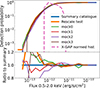 |
Fig. A.1. Detection probability as a function of X-ray flux. The collection of the four mocks processed with the standard pipeline is shown in blue, the rescale test is in orange. The individual mocks are displayed with thinner coloured lines. The pink line denotes the normalised histogram of the X-GAP fluxes. The bottom panel shows the ratio between each catalogue and the collection of the four mocks. |
Appendix B: Velocity dispersion and M500c
Compared to other galaxy clusters samples, the strength of X-GAP resides in mapping the gas properties out to R500c with high signal to noise ratio for low mass haloes hosting galaxy groups. Therefore, estimating the halo mass at larger radii, such as M200c is challenging. As explained in the main body of the article, we focus first on M200c to compare our results with previous works, since most of the literature focuses on R200c for such studies. In addition, we use our mock to calibrate the scaling relation between velocity dispersion and M500c. The formalism is the same as in Eq. 17, we simply substitute M200c with M500c. We fit for A, α, σintr, and σmeas. We put uniform priors on the parameters as reported in Table B.1.
Priors and posteriors of the scaling relation between halo mass M500c and velocity dispersion.
The results for the two cases using M200c or M500c are qualitatively similar. For the M500c case, we find a higher normalisation compared to the M200c case equal to A = 1332.2±5.2. This is expected, because the scaling relation is anchored at high mass of 1015 M⊙ and M500c is smaller than M200c. The slope α = 0.348±0.001 is slightly steeper, but compatible within the intrinsic scatter. The true intrinsic scatter σintr = 0.073±0.001 is compatible within 1σ with the M200c case. Similarly to the first case, the scatter is dominated by measurement uncertainty, with a σmeas = 0.102±0.001 and σmeas = 0.106±0.002 for the haloes detected in the optical and optical plus X-ray bands. Similarly to Fig. 11, the full relation between velocity dispersion and M500c is reported in Fig. B.1, with the top and bottom panels respectively showing the true and measured σV as a function of M500c. Similarly, the full posterior distributions are shown in Fig. B.2.
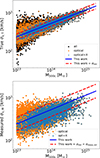 |
Fig. B.1. Scaling relation between velocity dispersion and halo mass M500c. The top and bottom panels are the same as in Fig. 11, but the reference mass is M500c instead of M200c. |
Appendix C: Selection impact on scaling relations
In this section we present the impact of the selection on the scaling relations between halo mass and observables, that is, temperature, luminosity, and velocity dispersion. In different mass bins, we compute the median observable, together with their 16th and 84th percentile points. We do it for the full population in the light cone and for the selected one after the optical and X-ray detection in our simulations. The result is collected in Fig. C.1. The top panels show the scaling relation rescaled by the self similar redshift evolution using E(z), the bottom panels display the ratio between the selected and the full population. We do not see an impact on the velocity dispersion to mass scaling relation, which confirms our previous findings in Sect. 5, with the X-ray selection being the limiting factor in our set-up, and Sect. 6, with similar best-fit parameters for the scaling relation before and after the selection. In addition, temperature does not impact the selection. The ratio between the selected and the full population is constant around 1. The same does not hold for luminosity. Moving towards lower masses, the selection is biased towards the brightest systems, with a 25% net effect 2×10¹³ M⊙. This is expected, because luminosity is the intrinsic property related to the observable that mostly impact our detection probability, that is, flux (see Sect. 5).
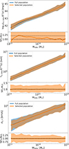 |
Fig. C.1. Scaling relation between observables and halo mass M500c. The top panel shows the X-ray luminosity, the central one displays temperature, while the bottom one reports the velocity dispersion. |
We further investigate this trend by dividing our samples into multiple redshift bins. The result is shown in Fig. C.2, where the redshift intervals are encoded in different colours: below 0.06 (in blue and orange), then up to 0.1 (in green and red), and 0.15 (in purple and brown). The bottom panel shows the ratio between the two populations in each bin, that is, the orange (red, brown) line is divided by the reference blue (green, purple) one. We find that the low redshift population is the least biased. The ratio between the full and the selected population is close to one down to 4×10¹³ M⊙, then it increases by about 20% down to about 1.5×10¹³ M⊙. As redshift increases, the detection of faint systems at fixed mass is more challenging and the scaling relation is more biased. In the middle redshift bins, there is 10% bias at 6×10¹³ M⊙, while in the higher redshift bin, the same bias is already reached at about 2×10¹⁴ M⊙. This highlights the importance of accounting for the selection function in this type of analysis, which are naturally affected by selection effects in extragalactic surveys.
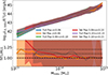 |
Fig. C.2. Scaling relation between X-ray luminosity and halo mass, as in the top panel of Fig. C.1, but split in different redshift bins. The panel shows the comparison between full population in the light cone and the one selected from our detection scheme. Different colours denote various redshift intervals: below 0.06 (in blue and orange), then up to 0.1 (in green and red), and 0.15 (in purple and brown). |
Appendix D: Self similar emission measure profile
We detail the calculation of the self similar emission measure profiles in this appendix. We start from a cluster surface brightness profile, defined as count rate in different radial bins per unit surface, that is, in units of cts/s/arcmin2. We can obtain the APEC normalisation profile by dividing the surface brightness profile by the net count rate obtained from xspec by assuming a Tbabs(APEC) model with the proper values of NH, temperature, redshift, metallicity and setting the normalisation to one, accounting for the response files of the instrument for the study (Eckert et al. 2012).
The APEC normalisation is defined as
![Mathematical equation: $$ {\mathrm {APEC NORM}} = \frac {10^{-14}}{4\pi [d_A (1+z)]^2} \int n_e n_H dV, [cm^{-5}] $$](/articles/aa/full_html/2025/07/aa53977-25/aa53977-25-eq53.gif) (D.1)
(D.1)
with dA being the angular diameter distance at redshift z. The self similar emission measure integrated along the line of sight is
 (D.2)
(D.2)
Combining equations D.1 e D.2 and splitting the volume integral between plane of the sky and line of sight we obtain
![Mathematical equation: $$ \begin{aligned}dV &= A \times dl \\ M &= \frac {10^{-14}}{4\pi [d_A (1+z)]^2} \\ N &= \sqrt {kT/10\ {\mathrm {keV}}} E(z)^3 \\ {\mathrm {APEC NORM}} &= M \times N \times EM \times A. \end{aligned} $$](/articles/aa/full_html/2025/07/aa53977-25/aa53977-25-eq55.gif) (D.3)
(D.3)
Considering an area A of 1 arcmin2 and the corresponding solid angle Ω with the proper conversion from arcmin to rad, we have
 (D.4)
(D.4)
Substituting equation D.4 into D.3 we get
 (D.5)
(D.5)
which we can invert to derive the final expression to infer the self similar emission measure profile from the APEC normalisation:
 (D.6)
(D.6)
All Tables
Priors and posteriors of the scaling relation between halo mass M200c and velocity dispersion.
Priors and posteriors of the scaling relation between halo mass M500c and velocity dispersion.
All Figures
|
Fig. 1. Forward-modelling of the X-GAP selection. We started from a dark matter halo light cone generated from the Uchuu simulation, built a novel method for assigning cluster and group X-ray profiles and temperatures as a function of the halo mass and redshift, and used abundance-matching schemes to simulate galaxies and AGN. We generated X-ray events and accounted for the telescope response. Finally, we reproduced the detection schemes in X-ray and optical bands to select an X-GAP-like sample from our simulation. |
| In the text | |
|
Fig. 2. Dark matter halo light cone generated from individual Uchuu snapshots. This panel shows a slice within ±50 Mpc along the z-axis up to redshift of 0.4. We show haloes more massive than 1012.5 M⊙ colour-coded by its redshift. The shaded areas denote the various snapshots we used to generate the light cone. |
| In the text | |
|
Fig. 3. Emission measure profiles with self-similar scaling, colour-coded for temperature, as a function of radius in units of R500c. The units on the y-axis are Mpc keV−1/2 cm−6. The bottom part of the panel shows the evolution of the intrinsic scatter of the profile at different radii. For reference, it is compared to the model from Comparat et al. (2020) and profiles of X-COP clusters (Ghirardini et al. 2019). |
| In the text | |
|
Fig. 4. X-ray scaling relation prediction of the cluster and group model. Top panel: Scaling relation between X-ray luminosity obtained by integrating the emission measure profiles (see Eq. (11)) and halo mass. Bottom panel: Scaling relation between temperature and halo mass. The blue shaded area shows the 16th–84th percentile distribution for the model applied to the Uchuu light cone in each mass bin. Our model is compared to a collection of real groups and cluster samples. The bottom part of both panels shows the intrinsic scatter evolution as a function of halo mass. |
| In the text | |
|
Fig. 5. Image example showing one of the brightest clusters in our mock with the additional components we included in the simulation. A secondary halo is located in the south-east region compared to the brightest one. The events generated by clusters (AGN, the X-ray background) are displayed as small dots in blue (orange, green). The true halo position is shown with large crosses, colour-coded by the X-ray flux. The position of the X-ray wavelet (optical FoF) detection is located at the cyan circle (magenta triangle). Each galaxy is marked by the small plus signs, according to their g-r colour. The vertical colour bar refers to input groups and clusters (the large crosses), the bottom one to individual galaxies (small plus signs). |
| In the text | |
|
Fig. 6. Scaling relation between X-ray luminosity and measured velocity dispersion. The result from our simulation (the real AXES) is shown in blue (orange). We find excellent agreement between the mock and real data in Damsted et al. (2024). |
| In the text | |
|
Fig. 7. Two-dimensional probability of detection for X-ray plus optically selected haloes in our simulation (see Sect. 5.1). The panels shows the completeness fraction as a function of three combinations of X-ray flux, velocity dispersion, and true velocity dispersion. |
| In the text | |
|
Fig. 8. Probability of detection for X-GAP-selected haloes as a function of observables. The three panels show different combinations of flux measured within R500c, redshift, and velocity dispersion on the x-axis in different colours and with different symbols. The various line styles denote the selection function model in Eq. (15). The error bars account for the Poisson error on the number of total and detected sources. The lines in each panel were shifted by −0.02, −0.01, 0, and 0.01 dex for clarity. |
| In the text | |
|
Fig. 9. Marginalised posterior distribution of the best-fit model of the X-ray plus optical selection function (see Eq. (15)). The filled 2D contours show the 1σ and 2σ confidence levels of the posteriors after convolution with the uniform priors. The green contours denote the base selection function where flux is measured within R500c, the violet contours show the effect of measuring flux within an angular aperture of six arcminutes. The parameter values are reported in Table 2. |
| In the text | |
|
Fig. 10. Trade-off between completeness and purity as a function of velocity dispersion. Left panel: Fraction of objects with a corresponding real input dark matter halo as a function of measured velocity dispersion. The blue line shows the fraction of objects detected in the optical mock that are matched to a real halo in the light cone. The orange line denotes objects with a corresponding X-ray detection. The green and red lines refer to the low redshift population, in the interval of interest for X-GAP, between 0.02 and 0.06. The black line shows the normalised distribution of measured velocity dispersion in the simulation. Central panel: Distribution of the measured velocity dispersion in our mock and in the real data. The blue and orange lines are left as a reference from the previous panel. The pink lines show the normalised distributions of the real AXES sample from Damsted et al. (2024), while the black ones refer to the simulation. The solid (dashed) lines denote the full optical (optical plus X-ray) detections. Right panel: Fraction of real input dark matter haloes with a corresponding detection in the mock. The coloured lines represent the same populations as the top panel, but starting from the true input dark matter haloes. |
| In the text | |
|
Fig. 11. Scaling relation between velocity dispersion and halo mass. Top panel: Scaling relation for the true velocity dispersion (Eq. (3)). The orange and green lines show the results from Munari et al. (2013) and Ferragamo et al. (2022). Bottom panel: Scaling relation for the measured velocity dispersion (Sect. 4.2). The blue line denotes the best-fit relation, and the red lines include the contribution of the intrinsic and measurement scatter summed in quadrature (see Eq. (17)). |
| In the text | |
|
Fig. 12. Marginalised posterior distributions of the best-fit scaling relation parameters between velocity dispersion and M200c. The filled 2D contours show the 1-σ and 2-σ confidence levels of the posteriors after convolution with the uniform priors. The model is given by Eq. (17). The corresponding 1D parameter constraints are reported in Table 3. The top panel refers to direct relation between true velocity dispersion and halo mass, with black contours referring to the full sample, orange ones to clusters and groups detected in the optical mock, and blue ones with the addition of the X-ray detection. The bottom panel refers to the full model of the scaling relation accounting for the measured velocity dispersion. |
| In the text | |
|
Fig. 13. Ratio of the measured and true velocity dispersion as a function of the number of recovered galaxy members. The red line shows the gapper velocity dispersion measured by the CLEAN algorithm, and the blue line refers to the direct estimate from the FoF finder. The dashed black line denotes the one-to-one ratio, and the dotted lines include a 10% deviation from unity. |
| In the text | |
|
Fig. 14. Probability of detection as a function of core properties. The dashed lines represent the normalised distribution of the full population. Top panel: Completeness fraction as a function of emissivity profile ratio measured at R500c and in the inner most bin. Different flux intervals are encoded in different colours. Bottom panel: Completeness fraction as a function of flux for the cool core (non-cool core) systems with profile ratio smaller (larger) than the median values of 0.001. |
| In the text | |
|
Fig. 15. Selection of relaxed and unrelaxed groups from the point of view of the dark matter halo ba sed on the spin and offset parameters. |
| In the text | |
|
Fig. 16. Full marginalised posterior distribution for the scaling relation between halo mass and velocity dispersion for relaxed and unrelaxed haloes. |
| In the text | |
|
Fig. 17. Average galaxy member distances from the halo centre as a function of halo mass. The blue line denoted relaxed haloes, and the red line refers to disturbed ones. |
| In the text | |
|
Fig. A.1. Detection probability as a function of X-ray flux. The collection of the four mocks processed with the standard pipeline is shown in blue, the rescale test is in orange. The individual mocks are displayed with thinner coloured lines. The pink line denotes the normalised histogram of the X-GAP fluxes. The bottom panel shows the ratio between each catalogue and the collection of the four mocks. |
| In the text | |
|
Fig. B.1. Scaling relation between velocity dispersion and halo mass M500c. The top and bottom panels are the same as in Fig. 11, but the reference mass is M500c instead of M200c. |
| In the text | |
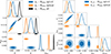 |
Fig. B.2. Same as Fig. 12, but referring to the scaling relation to M500c. |
| In the text | |
|
Fig. C.1. Scaling relation between observables and halo mass M500c. The top panel shows the X-ray luminosity, the central one displays temperature, while the bottom one reports the velocity dispersion. |
| In the text | |
|
Fig. C.2. Scaling relation between X-ray luminosity and halo mass, as in the top panel of Fig. C.1, but split in different redshift bins. The panel shows the comparison between full population in the light cone and the one selected from our detection scheme. Different colours denote various redshift intervals: below 0.06 (in blue and orange), then up to 0.1 (in green and red), and 0.15 (in purple and brown). |
| In the text | |
Current usage metrics show cumulative count of Article Views (full-text article views including HTML views, PDF and ePub downloads, according to the available data) and Abstracts Views on Vision4Press platform.
Data correspond to usage on the plateform after 2015. The current usage metrics is available 48-96 hours after online publication and is updated daily on week days.
Initial download of the metrics may take a while.