| Issue |
A&A
Volume 697, May 2025
|
|
|---|---|---|
| Article Number | A226 | |
| Number of page(s) | 23 | |
| Section | Cosmology (including clusters of galaxies) | |
| DOI | https://doi.org/10.1051/0004-6361/202453086 | |
| Published online | 22 May 2025 | |
Investigating the galaxy–halo connection of DESI emission-line galaxies with SHAMe-SF
1
Donostia International Physics Center (DIPC), Donostia-San Sebastian, Spain
2
University of the Basque Country UPV/EHU, Department of Theoretical Physics, Bilbao E-48080, Spain
3
IKERBASQUE, Basque Foundation for Science, 48013 Bilbao, Spain
4
Institut de Física d’Altes Energies (IFAE), The Barcelona Institute of Science and Technology, 08193 Bellaterra (Barcelona), Spain
⋆ Corresponding author; This email address is being protected from spambots. You need JavaScript enabled to view it.
Received:
20
November
2024
Accepted:
13
February
2025
Abstract
Context. The Dark Energy Spectroscopic Instrument (DESI) survey is mapping the large-scale distribution of millions of emission line galaxies (ELGs) over vast cosmic volumes to measure the growth history of the Universe. However, compared to luminous red galaxies, it is more complex to model the connection of ELGs with the underlying matter field.
Aims. We employed a novel theoretical model, SHAMe-SF, to infer the connection between ELGs and their host dark matter haloes and subhaloes. SHAMe-SF is a version of subhalo abundance matching that incorporates prescriptions for multiple processes, including star formation, tidal stripping, environmental correlations, and quenching.
Methods. We analysed public measurements of the projected and redshift-space ELG correlation functions at z = 1.0 and z = 1.3 from the DESI One Percent data release (from the Early Data Release), which we fitted over a broad range of scales, r ∈ [0.1, 30]/h−1 Mpc, to within the statistical uncertainties of the data. We also validated the inference pipeline using two mock DESI-ELG catalogues built from hydrodynamic (TNG300) and semi-analytic galaxy formation models (L-Galaxies).
Results. SHAMe-SF is able to reproduce the clustering of DESI ELGs and the mock DESI samples within statistical uncertainties. We infer that DESI ELGs typically reside in haloes of ∼ 1011.8 h−1 M⊙ when they are centrals and ∼ 1012.5 h−1 M⊙ when they are satellites, which occurs in ∼30% of cases. In addition, compared to the distribution of dark matter within haloes, satellite ELGs preferentially reside both in the outskirts and inside haloes, and have a net infall velocity towards the centre. Finally, our results show evidence of assembly bias and conformity. All these findings are in qualitative agreement with the mock DESI catalogues.
Conclusions. These results pave the way for a cosmological interpretation of DESI ELG measurements on small scales using SHAMe-SF.
Key words: galaxies: formation / galaxies: statistics / large-scale structure of Universe
© The Authors 2025
 Open Access article, published by EDP Sciences, under the terms of the Creative Commons Attribution License (https://creativecommons.org/licenses/by/4.0), which permits unrestricted use, distribution, and reproduction in any medium, provided the original work is properly cited.
This article is published in open access under the Subscribe to Open model. This email address is being protected from spambots. You need JavaScript enabled to view it. to support open access publication.
1. Introduction
Current galaxy surveys are mapping the large-scale structure of the Universe across a wide redshift range, seeking new insights into the nature of our Universe and its components. In the redshift range 0.8 < z < 1.6, emission line galaxies (ELGs) are an ideal target for these surveys because of their high number density and characteristic spectral features. One such survey, the Dark Energy Spectroscopic Instrument (DESI) survey (DESI Collaboration 2016), recently released the first 1% of its data, collecting spectra from ∼250 000 ELGs identified using the [OII] line doublet (DESI Collaboration 2024a). This number is already similar to that of eBOSS (Extended Baryon Oscillation Spectroscopic Survey), which had been the largest ELG survey (e.g. Raichoor et al. 2016).
To maximally exploit the data provided by surveys like DESI, it is necessary to link the observed galaxies with the underlying dark-matter field. Understanding this connection and the properties of the observed galaxies enables the creation of more realistic mocks and the development of more accurate theoretical models (Cuesta-Lazaro et al. 2023; Chaves-Montero et al. 2023; Contreras et al. 2023a). Several analyses of semi-analytic models (SAMs; Gonzalez-Perez et al. 2018, 2020) and hydrodynamic simulations (Hadzhiyska et al. 2021; Yuan et al. 2022a) have characterised ELGs as galaxies with high (specific) star formation rates (SFRs) that inhabit intermediate-mass haloes, with ∼10% of them being passive galaxies that host an active galactic nucleus (AGN). This is supported by observational studies at redshifts 0.02 < z < 0.22 (Favole et al. 2024) and 0.8 < z < 1 (Yuan et al. 2023).
Previous analyses of the galaxy clustering of DESI and other ELG samples modelled the galaxy–halo connection using halo occupation distributions (HODs) and subhalo abundance matching (SHAM). Both are empirical models that select, based on their properties, which haloes or subhaloes host the galaxies of a given sample (see e.g. Wechsler & Tinker 2018, for a review). Even within the same family of models, the assumptions made for the galaxy–halo connection can be completely different.
Halo occupation distributions (Jing et al. 1998; Benson et al. 2000; Peacock & Smith 2000; Berlind et al. 2003; Zheng et al. 2005, 2007; Guo et al. 2015; Contreras & Zehavi 2023) model the probability distribution of finding a central galaxy and the number of satellite galaxies as a function of their host halo mass. To improve their accuracy at describing ELG samples, HODs underwent several extensions and modifications; for instance, they adopted functional forms and scatter around the mean (Jiménez et al. 2019; Alam et al. 2020; Rocher et al. 2023; Hadzhiyska et al. 2023a; Vos-Ginés et al. 2024; Garcia-Quintero et al. 2025), included secondary properties (Hearin et al. 2016; Hadzhiyska et al. 2023a), or altered the satellite phase-space distribution (e.g. Avila et al. 2020; Rocher et al. 2023). In addition to these changes, to reproduce the small-scale clustering of ELGs, state-of-the-art HODs also include conditional probabilities for satellites based on the type of their central galaxy (Alam et al. 2020; Yuan et al. 2023; Reyes-Peraza et al. 2024).
Standard SHAM (Vale & Ostriker 2006; Shankar et al. 2006; Conroy et al. 2006; Trujillo-Gomez et al. 2011) assumes that the most massive haloes host the most luminous galaxies. In the case of ELGs at redshifts below z = 2, this relation does not hold since the highest star-forming galaxies do not usually populate the highest-mass subhaloes (e.g. Gonzalez-Perez et al. 2018). SHAM can account for this by changing the subhalo selection criteria (Favole et al. 2016; Prada et al. 2025; Yu et al. 2024). Extended SHAM also regulates the number of satellites in the sample, using the satellite fraction as a free parameter. Other approaches first perform a SHAM to model stellar mass and then select ELGs using a secondary subhalo property (Favole et al. 2022; Lin et al. 2023) or by selecting from a set of ELG candidates (Gao et al. 2022, 2023). In the latter approach, the satellite fraction is regulated by an additional free parameter (Gao et al. 2024) and correlations between centrals and their satellites (an effect known as ‘conformity’) are included, which improve the modelling of galaxy clustering on scales below 0.3 h−1 Mpc.
In a previous paper (Ortega-Martinez et al. 2024), we presented SubHalo Abundance Matching extended–Star Formation (SHAMe-SF), a new model for ELGs and star-forming samples, which we extensively validated using a hydrodynamic simulation and a SAM. Here, we apply the SHAMe-SF model to ELG data from DESI’s One Percent data release (DESI Collaboration 2024a). Our model can accurately reproduce galaxy clustering on small scales (r ∈ [0.1, 30]/h−1 Mpc). After fitting the clustering, we computed the posterior predictive distribution of the host halo mass distribution, assembly bias, satellite fractions, and phase-space distribution. We find that central ELGs are hosted by haloes with average masses of 1011.8 h−1 M⊙ if they are central, and 1012.5 h−1 M⊙ if they are satellites, and their clustering depends on properties beyond halo mass. Satellites are distributed almost isotropically, and we can divide them into an infalling population (outside the halo boundary with negative radial velocities) and an orbiting population. Even if most satellites inhabit haloes where the central galaxy is not an ELG, some haloes with lower halo masses (1012.2 h−1 M⊙) are conformal. SHAMe-SF’s capability to make this prediction was validated using two mock DESI samples built using a hydrodynamic simulation and a SAM. We also compared our findings with other models applied to DESI ELGs, finding good agreement for all the aspects of the galaxy–halo connection we analysed, except the satellite fractions.
This paper is structured as follows: A detailed description of the observational data, the choice of the validation mock DESI ELG samples, and the simulations used in this work are given in Sect. 2. We describe the SHAMe-SF model and the galaxy clustering statistics in Sect. 3. We use these tools in Sect. 4 to fit the galaxy clustering of DESI’s ELGs in the redshift ranges 0.8 < z < 1.1 and 1.1 < z < 1.6. Finally, our inference on the galaxy–(sub)halo connection is reported in Sect. 5. We compare these results with other ELG analyses in Sect. 6. Our conclusions are summarised in Sect. 7.
2. Observational and mock data
In this section we describe the different datasets we employed. First, we provide details on the ELG samples observed by DESI (Sect. 2.1). Then, we describe the simulation (TNG300, the largest box from the IllustrisTNG simulation suite) and the SAM we employed to build mock DESI ELG catalogues (Sect. 2.2).
2.1. ELGs in the DESI One Percent data release
In June 2023, the DESI collaboration released the first 1% of their data (DESI Collaboration 2024a) – the last step of its Survey Validation programme (DESI Collaboration 2024b). The sky area scanned consisted of 140 sq deg, made of 20 non-overlapping rosettes with repeated observations to maximise the number of observed galaxies (due to fibre assignment) with reliable redshift estimations.
These data contain a sample of ELGs, over the redshift range 0.6 < z < 1.6, with a selection criteria similar to that planned for the complete DESI survey (DESI Collaboration 2016; Raichoor et al. 2020, 2023). These galaxies were selected photometrically (via magnitude and colour cuts) and later confirmed spectroscopically by identifying the [O II] doublet in their spectra. Overall, the success rate of the target selection reached ∼90% (DESI Collaboration 2024a). Despite the limited volume, this dataset represents a unique opportunity to learn about ELGs at high redshift and their connection with the underlying dark matter.
Here, we employed public measurements of the clustering of these ELGs provided by the DESI collaboration (Rocher et al. 2023). The ELG sample was divided into a low-z and a high-z bin: z ∈ [0.8, 1.1] and z ∈ [1.1, 1.6]. The clustering measurements cover a wide range of scales, r ∈ [0.1, 30] h−1 Mpc, and have been corrected for observational systematic effects such as incompleteness and density inhomogeneities originating from fibre assignment. We also employed the covariance matrices provided by DESI. As described in Rocher et al. (2023); diagonal elements were estimated using a jackknife method and off-diagonal elements using a suite of HOD catalogues.
The [O II] emission of some galaxies in the DESI ELG sample can come from AGNs instead of star formation. This fraction is estimated to be very low (∼4%; Lan et al. 2024); thus, we do not expect this to affect our results significantly.
2.2. Mock DESI catalogues
We built two mock catalogues based on the TNG300 hydrodynamic simulation and a SAM to validate and interpret our results. In hydrodynamic simulations, baryons and gravity are jointly evolved. Semi-analytic models use the merger trees of dark matter-only simulation to model the evolution of the baryonic components of galaxies (for a review, see Baugh 2006; Benson 2010).
2.2.1. Galaxy formation simulations
TNG300 is a large publicly available high-resolution hydrodynamic simulation, which evolves dark matter, gas, stars, and black holes inside a periodic box of 205 h−1 Mpc (∼300 Mpc; Nelson et al. 2018; Springel et al. 2018; Marinacci et al. 2018; Pillepich et al. 2018; Naiman et al. 2018). Compared to observations, TNG300 reproduces the stellar mass function from SDSS (Sloan Digital Sky Survey, Pillepich et al. 2018, Jackson et al. 2020), as well as the stellar mass–SFR main sequence and the scatter on this relation (Donnari et al. 2019).
On the other hand, several aspects of the galaxy population are not reproduced by TNG300. Additionally, it has not been calibrated to match the observed properties of ELGs. For these reasons, we employed another galaxy formation model, namely the L-Galaxies SAM, with which we estimated the current modelling uncertainties and validated our inferences in two different galaxy formation scenarios.
We employed the catalogues provided by Ayromlou et al. (2021). These catalogues were generated using the Henriques et al. (2015) version of L-Galaxies on top of the subhalo merger trees extracted from a gravity-only version of the TNG300. As for the TNG300, it has been extensively tested that L-Galaxies reproduces multiple aspects of the observed galaxy population (Guo et al. 2011, 2013; Henriques et al. 2013, 2020).
2.2.2. ELG selection
DESI employs photometric selections to identify ELG candidates. Using the same criteria to build the mock DESI ELG catalogues using TNG300 and L-Galaxies implies modelling of additional processes (such as dust obscuration, metallicities, or burstiness), to obtain realistic colour-colour distributions. Instead, we defined our mock DESI ELG samples based on the stellar masses and SFRs of galaxies.
Yuan et al. (2023) estimated the stellar masses and SFRs of DESI ELGs in the redshift interval 0.8 < z < 1.1 by cross-matching them with galaxies in the COSMOS (The Cosmic Evolution Survey) survey (Weaver et al. 2022). Yuan et al. (2023) show that DESI ELGs populate a well-defined region in terms of the SFR, M*, and specific SFR (sSFR). Specifically, these galaxies lie above the main sequence, have a minimum SFR of ∼ 1 M⊙ yr−1, a minimum stellar mass of 108.7 M⊙, and a maximum stellar mass of 1010.5 M⊙, and therefore none are massive quenched galaxies.
Similar to Fig. 5 in Yuan et al. (2023), in Fig. 1 we show the distribution of SFRs and stellar masses (M*) for galaxies in the TNG300 simulation and L-Galaxies SAM catalogues (orange and blue contours, respectively). We note that this is the only case where mass units are M⊙ and not h−1 M⊙ to ease the comparison with the crossmatch with COSMOS. Although the two models are broadly consistent, we can see some differences. TNG300 shows a more narrowly defined main sequence of star formation and a drastic quenching at log(M*/M⊙)∼10.5. In contrast, quenching is less evident in the SAM for higher halo masses.
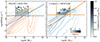 |
Fig. 1. Distribution of stellar masses (M*) and SFRs for galaxies at z = 1 as predicted by the TNG300 hydrodynamic simulation (‘DESI-TNG’, left panel) and by the L-Galaxies semi-analytic galaxy formation model (‘DESI-SAM’, right panel). Our mock DESI samples are defined by selection criteria for M*, SFRs, and the main sequence (similar to a cut in the sSFR), as indicated by solid lines (see Fig. 5 of Yuan et al. 2023 for a crossmatch between observed DESI and COSMOS galaxies). Note that the units for stellar mass are M⊙ (without the h factor). The fraction of selected galaxies for such samples is shown in a grey scale. |
To mimic these constraints in our mocks, we first matched COSMOS’s cumulative stellar mass and SFR functions with those in either TNG300 or L-Galaxies. We then defined thresholds that would yield the same abundance of galaxies. Subsequently, we fitted the M*-SFR main sequence in each catalogue and discarded galaxies below it. We call the final catalogues DESI-TNG (for the hydrodynamic simulation) and DESI-SAM (for the SAM). Finally, we down-sampled each catalogue to match DESI’s number density ( ; by a factor of ∼4 for DESI-TNG and ∼3 for DESI-SAM). This down-sampling mimics the incompleteness of the selection criteria. The final selection thresholds are indicated as blue (DESI-TNG) and orange (DESI-SAM) solid lines in Fig. 1. The grey colour bar indicates the fraction of galaxies in the ELG catalogues.
2.3. A note on halo finders
Throughout this work, we distinguish between subhaloes and haloes and between centrals and satellites. When comparing our inferences to other DESI models, it is important to consider the difference between halo finders when identifying different structures. Both the TNG and BACCO1 simulations use FoF (Davis et al. 1985) and SUBFIND (Springel et al. 2001) to define structures.
The FoF algorithm groups particles together based on a fixed length scale known as the linking length, which is usually set to a fraction of the mean inter-particle separation in the simulation. In contrast, SUBFIND identifies (sub-)structures based on the topology of the density field by identifying saddle points in the latter. In this work, we refer to all structures identified by SUBFIND as subhaloes. We note that this also includes a central subhalo consisting of most of the host halo from which we removed all particles belonging to other subhaloes. These secondary subhaloes are then considered to be satellites.
In Sect. 6 we compare our inferences to other works from the DESI collaboration. In most cases, the halo finder of choice is Rockstar (Behroozi et al. 2013) This halo finder performs an initial group division using a 3D FoF inspired algorithm with a large linking length, and identifies structures and substructures within each group through distances in 6D phase space. Further comparisons of halo finders are provided in Knebe et al. (2011), Onions et al. (2012), and Pujol et al. (2014). The main difference affecting our comparison is the labelling of structures outside of r200c. FoF + SUBFIND labels some substructures as satellites of a larger halo (see Hadzhiyska et al. 2023a), while Rockstar identifies the same structures as separate haloes. We note that this is relevant when analysing satellite fractions predicted by different models, and is taken into consideration in Sect. 6.3.1.
3. SHAMe-SF galaxy population model
In this section we recap our model for the clustering of ELG and describe the gravity-only simulation with which we computed its predictions. Then, we describe an emulator we built to accelerate the evaluation of model predictions.
3.1. SHAMe-SF
SHAMe-SF is based on the SHAM formalism and includes physical prescriptions to link the SFR of a galaxy to the properties of its host subhalo. The model was first presented in Ortega-Martinez et al. (2024), where we refer the reader to for an extensive discussion of the main ingredients and assumptions. In short, the SFR of a galaxy is assumed to be a function of the peak circular velocity, Vmax, of the host’s dark matter subhalo, where nuisance parameters control the functional form, scatter, and secondary correlations (using subhalo concentration). The SFR is also suppressed as a function of the host halo mass and time since accretion, effectively modelling gas stripping and quenching. Here, and in the remainder of the paper, we define the halo mass, Mh, as the mass contained within a sphere of an average density 200 times the critical density of the universe and centred in the minimum of the gravitational potential (whose radius is defined as r200c). We took the satellite definition from FoF (Davis et al. 1985) + SUBFIND (Springel et al. 2001), which also considers satellites beyond r200c.
For this work, we extended SHAMe-SF to allow an increase in SFR for very massive galaxies. Specifically, the SFR is given by
![Mathematical equation: $$ \begin{aligned} \mathrm{SFR}|_{({V_{\rm peak}})} \propto {\left\{ \begin{array}{ll} \left[ \left( \frac{V_{\rm peak}}{V_{1}}\right)^{-\beta } + \left( \frac{V_{\rm peak}}{V_{1}}\right)^{\gamma } \right]^{-1},&\mathrm{if}\ V_{\rm peak} \le V_{1}+\Delta V_1\\&\\ \mathrm{SFR}_{V_{1}+\Delta V_1} \left.\ \left( \frac{V_{\rm peak}}{V_{1}+\Delta V_1}\right)^{\gamma + \Delta \gamma } \ \right.\&\mathrm{if}\ V_{\rm peak} > V_{1}+\Delta V_1 \end{array}\right.} ,\end{aligned} $$](/articles/aa/full_html/2025/05/aa53086-24/aa53086-24-eq2.gif) (1)
(1)
where ΔV1 and Δγ are two additional free parameters compared to the original version of the model. SFRV1 + ΔV1 is a normalisation factor set to make the function continuous at SFRV1 + ΔV1. The option of including an additional feature in the functional form for high values of Vpeak was already discussed when we first presented the SHAMe-SF model. This term accounts for the possible connections between SFR and Vpeak that could appear due to different implementations of quenching and environmental effects (e.g. Contreras et al. 2015; Popesso et al. 2015; Nusser et al. 2020), as well as galaxies classified as ELG due to AGN emission lines rather than SF-related lines.
In the first version of SHAMe-SF, the same parameter regulated the secondary dependence on Vpeak/Vvir for centrals and satellites (fk). In this version, we used the same parameterisation as in Contreras et al. (2023a) and allowed for different dependences (fk, cen and fk, sat). This separation can describe differences between centrals and satellites depending on concentration that are not already captured by the quenching mechanism dependent on host halo mass and time since peak mass. To select a sample with a given number density  on a simulation with co-moving volume, V, we selected the
  subhaloes with the highest SFR (given by the relation with Vpeak, the semi-sorted scatter and the suppression in terms of the host halo mass).
The original version of the model was validated against multiple catalogues of SFR-selected galaxies extracted from the TNG and a SAM model (Ortega-Martinez et al. 2024). Specifically, SHAMe-SF was able to fit the projected and redshift-space clustering of ELGs with number densities over the range  at z = 0 and 1. Here, we further validated the extended version of the model against the mock DESI ELG catalogues described previously. In Appendix A we display our results, showing that SHAMe-SF can successfully fit the clustering statistics and provide accurate inferences about the galaxy-halo connection of mock DESI ELGs.
3.2. Gravity-only simulations
To suppress the impact of cosmic variance, we computed the predictions of SHAMe-SF on a simulation much larger than that employed for building our mock DESI ELG catalogues. Specifically, we used three gravity-only simulations of the BACCO simulation project (Angulo et al. 2021). The first simulation evolved 15363 particles of mp = 109.5 h−1 M⊙ on a box of 512 h−1 Mpc a side, which we employed to evaluate SHAMe-SF models. We used the other two simulations (with paired phases), with 30723 particles on a 1024 h−1 Mpc, to construct a SHAMe-SF emulator. The cosmology adopted by both simulations corresponds to the best-fit analysis of the Planck satellite data (Planck Collaboration XIII 2016): Ωm = 0.3089, σ8 = 0.8159, ns = 0.9667 and h = 0.6774, which is, hence, the fiducial cosmology adopted throughout our analyses.
The initial conditions of our simulations were computed using 2LPT (Second-order Lagrangian Perturbation Theory), where mode amplitudes were fixed to the ensemble average, drastically suppressing variance on large scales (Angulo & Pontzen 2016). Similarly to other BACCO simulations, we identified on-the-fly haloes and subhaloes using FoF and SUBFIND algorithms, respectively (Davis et al. 1985; Springel et al. 2001), as well as all the dark matter properties that SHAMe-SF requires.
3.3. A SHAMe-SF emulator
Following Angulo et al. (2021), we sped up the evaluation of SHAMe-SF predictions by building a simple feed-forward neural network emulator (see also Aricò et al. 2021, 2020; Pellejero Ibañez et al. 2023; Zennaro et al. 2023; Contreras et al. 2023a; Ortega-Martinez et al. 2024). We started by defining the set of SHAMe-SF parameter combinations, randomly distributed according to a Latin hypercube over the ranges
![Mathematical equation: $$ \begin{aligned} \beta&\in [0,20]\nonumber \\ \gamma&\in [-15,25] \nonumber \\ \Delta \gamma&\in [-10,10] \nonumber \\ V_1&\in [10^{1.8},10^{3.2}]\,\mathrm{(km/s)} \nonumber \\ \Delta V_1&\in [10^{0.2},10^{1.9}]\,\mathrm{(km/s)} \nonumber \\ \sigma&\in [0,2] \\ f_{k,\mathrm{(cen+sat)/2}}&\in [-1,1] \nonumber \\ f_{k,\mathrm{(cen-sat)/2}}&\in [-1,1] \nonumber \\ \alpha _0&\in [0,8] \nonumber \\ \alpha _{\rm exp}&\in [-8,8] \nonumber \\ M_{\rm crit}&\in [8.5,15] \ (\log (h^{-1}\,\mathrm{M}_{\odot })), \end{aligned} $$](/articles/aa/full_html/2025/05/aa53086-24/aa53086-24-eq6.gif) (2)
(2)
where {β, γ, Δγ, ΔV1, σ} describe the relation between SFR and circular velocity, {fk, (cen + sat)/2, fk, (cen − sat)/2} control the correlation with concentration, {α0, αexp, Mcrit} regulate the impact of gas stripping in satellites. These ranges are motivated by the analysis of star-forming galaxies from TNG300 and L-Galaxies in Ortega-Martinez et al. (2024) and are wide enough to avoid truncating the posterior distributions. We refer to Ortega-Martinez et al. (2024) for further details on the relation between parameters.
We then evaluated SHAMe-SF on top of our 1 h3 Gpc−3 gravity-only simulation at 10 redshifts over the range z ∈ [0.8, 1.6]2 and for six number density thresholds ![Mathematical equation: $ \bar{n} \in [10^{-4}, 10^{-2.5}]\,h^{3}\,\mathrm{Mpc}^{-3} $](/articles/aa/full_html/2025/05/aa53086-24/aa53086-24-eq7.gif) (equally spaced in log scale). Each evaluation takes approximately 20 CPU minutes (including calculating the galaxy clustering for the eight number densities).
(equally spaced in log scale). Each evaluation takes approximately 20 CPU minutes (including calculating the galaxy clustering for the eight number densities).
For each catalogue, we used CORRFUNC (Sinha 2016; Sinha & Garrison 2017) to compute the redshift-space 2D correlation function ξ(s, μ), where s2 = rp2 + rπ2 and  . To reduce statistical noise, we averaged the measurements over the three Cartesian axes and for eight model evaluations adopting different random seeds.
We computed the projected correlation function as follows:
 (3)
(3)
using the same separation bins and line-of-sight integration limit (πmax = 40 h−1 Mpc) as those used by DESI (Rocher et al. 2023). Subsequently, we estimated the multipoles of the correlation function as
 (4)
(4)
where Pℓ is the ℓ-th order Legendre polynomial.
Overall, by considering the different redshifts, number densities, and combinations of the SHAMe parameters, we obtained 130 000 measurements for each clustering statistic. We combined the data from different redshifts and number densities to train one neural network per clustering statistic. The architecture of the neural network is similar to that used in Contreras et al. (2023a): three fully connected hidden layers with 200 neurons. Variations in the architecture of the emulator do not significantly change our results. We used the TensorFlow library’s Keras front-end with the Adam optimisation algorithm, setting the learning rate to 0.001 and choosing a mean squared error loss function. 10% of the dataset was kept for validation.
4. Fitting DESI ELG clustering
This section discusses the fitting of DESI ELG clustering measurements using our SHAMe-SF model.
4.1. Likelihood, parameter space, and sampling
We assumed that the likelihood of observing a set of clustering statistics  is given by a multivariate Gaussian:
  , where t is the SHAMe-SF emulator predictions for a given set of parameters θ. We used the data vector, d, and covariance matrix, 𝒞−1, provided by the DESI collaboration (see Sect. 2.1). We included the emulator uncertainty (see Sect. 3.3) as an additive contribution to the diagonal of the covariance matrix.
We fixed the cosmological parameters to those assumed in our gravity-only simulation (see Sect. 3.2). Thus, we only varied parameters that control the relationship between ELGs and the host dark matter subhaloes. For all 11 SHAMe-SF parameters, we adopted flat priors over an interval that coincides with the ranges employed by our emulator. In Appendix A we show that these ranges comfortably enclose the values expected in the DESI-SAM and DESI-TNG ELG mocks. Thus, we expect these priors to be uninformative and not to affect our results. We note that our SHAMe-SF predictions assume values for Planck cosmology that do not match the fiducial cosmology assumed by DESI to transform angular separations and redshifts into distances. In principle, we could apply the so-called Alcock-Paczynski corrections after each model evaluation to account for this. However, the difference in cosmology is small (ΔΩm = 0.006); we verified that this effect negligibly impacts our predictions and, therefore, ignored it.
We separately analysed the low-z and high-z ELG samples. In each case, we evaluated SHAMe-SF at the median redshift of each sample (0.95 and 1.33, respectively). We only considered separations in the range r ∈ [0.1, 30] h−1 Mpc. The lower limit is set by the minimum scale for which we expect SHAMe-SF to deliver accurate inferences. The upper limit is set by the largest scale included in the public measurements, which also roughly coincides with the largest scale where the effect of the finite size of our gravity-only simulation is still small. Although not shown here, we verified that none of our results strongly depend on the minimum or maximum scale included in the fit.
We sampled the likelihood using an ensemble Markov chain Monte Carlo (MCMC) algorithm implemented by emcee (Foreman-Mackey et al. 2013). We employed a configuration consisting of 5000 chains, each with 30 000 steps. We note that the high computational efficiency of our emulator allows us to obtain 100 000 model evaluations in under 2 seconds of CPU time. Throughout this work, we refer to best-fit parameters as those that maximise the likelihood, and 1 and 2σ regions as 68 and 95% of the posterior distribution.
4.2. Best fit to DESI galaxy clustering
In Fig. 2 we display the measured projected correlation function and the monopole and quadrupole of the redshift space correlation function of the low-z and high-z DESI ELG samples. The best-fit SHAMe-SF model is shown as solid lines.
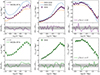 |
Fig. 2. Projected correlation function (wp) and the monopole (ξℓ = 0) and quadrupole (ξℓ = 2) of the redshift–space correlation function of ELGs in DESI at z = 0.95 (top row) and at z = 1.33 (bottom row), together with the corresponding best-fit SHAMe-SF model (purple and green lines). Bottom panels: Difference between the data and the fit with SHAMe-SF in units of the diagonal elements of the respective covariance matrix. For comparison, we display the measurements for our DESI-TNG and DESI-SAM mock DESI catalogues at z = 1 as blue and orange lines, respectively. SHAMe-SF is a reasonably good description of the data for all the statistics and scales considered. Note that the data display fluctuations inconsistent with the error bars, which suggests there could be sources of noise that are not accounted for in the covariance matrices. |
Firstly, we highlight that our model is an excellent description of the high- and low-z data over the whole range of scales considered. However, we note that the value of the reduced χ2, displayed in the legend, is somewhat high. Looking at the bottom panels, which display the difference between the data and the model in units of the diagonal elements of the covariance matrix, we can see no large systematic deviations from 0, typically the signature of model errors. Instead, there seem to be large random fluctuations, especially considering that neighbouring data points should exhibit a considerable degree of correlation. This suggests that there could be additional sources of stochastic noise or that the jackknife method (employed by DESI to estimate the covariance matrix) underestimates the actual uncertainty in the data.
In the case of the low-z sample, for which we have the crossmatch with COSMOS from Yuan et al. (2023), we can directly compare the DESI ELG clustering with that in our mock DESI-TNG and DESI-SAM catalogues (shown as dashed lines). We can see that for all statistics, the ELG mocks bracket the DESI measurements3, which indirectly supports the validity of our procedure to create DESI mocks to deliver plausible predictions for the galaxy–halo connection. The TNG-based sample is about 10% more biased, whereas the DESI-SAM is 2% less biased. This naively implies that the DESI-TNG (DESI-SAM) predicts more (fewer) satellites than measured in DESI, and a higher (lower) average mass for centrals (or satellite host halo mass). In subsequent sections, we explicitly explore this.
4.3. Constraints on SHAMe-SF model parameters
By fitting the clustering of DESI ELGs, we have constrained the free parameters of our SHAMe-SF model. In Fig. 3 we display the posterior distribution function on the four parameters best constrained by the data, namely: V1, the pivot value of Vmax, above which galaxies start to be quenched; fk, cen and fk, sat, which control the secondary dependence on subhalo concentration; and Mcrit, the host halo mass at which the SFRs of satellites decrease due to gas stripping. The full posteriors on the 11 parameters are shown in Fig. B.2.
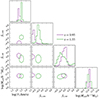 |
Fig. 3. Marginalised 1σ constraints on the most important SHAMe-SF parameters, obtained from fitting the clustering of DESI ELGs at z = 0.95 (purple) and 1.33 (green). |
First, the low and high-z samples prefer statistically consistent values for these SHAMe-SF parameters. This implies that the galaxy formation physics controlling ELGs does not significantly evolve between z = 1.0 and 1.3. Specifically, we obtain log V1 [km/s] ∼ 2.3: the SFR scales with Vpeak until subhaloes reach Vpeak ∼ 200 km/sec, after they start to be quenched for higher Vpeak values. Additionally, from the value of the Mcrit parameter, we infer that satellite ELGs are already affected by stripping in haloes of 1012 h−1 M⊙. The value of the ordering parameter for centrals (fk, cen) is negative for both redshift bins. For a fixed value of Vpeak, SHAMe-SF preferentially populates central subhaloes with lower concentrations. This is also true for satellites (fk, sat), but we find values closer to zero for the lower-z bin (almost random ordering). The next section explores what this implies for the type of dark matter structures DESI ELGs are located in.
5. Galaxy–halo connection in DESI ELGs
In this section we present the main results of our paper: constraints on the connection between DESI ELGs and the underlying dark matter structures. We explore the halo occupation number (Sect. 5.1), assembly bias (Sect 5.2) and the abundance and distribution of satellites (Sect. 5.3).
We obtained our inferences by randomly selecting 100 steps from our MCMC chains after discarding 10 000 burn-in steps. We then employed those parameter sets to build SHAMe-SF catalogues from our 512 h−1 Mpc gravity-only simulation. Finally, we computed the statistic of interest and present the median and 16th–84th percentiles of the distributions. We validated our procedure by applying it to our mock DESI catalogues, as shown in Appendix A.
5.1. Halo occupation number
In Fig. 4 we present our inferences on the average number of ELGs per halo as a function of halo mass for the low-z (left, purple) and high-z (right, green) samples. We find that central ELGs populate on average haloes of mass log(Mh/h−1 M⊙) = 11.7 ± 0.1 and 11.9 ± 0.1 in the low-z and high-z bins, respectively. For the mock ELG samples (DESI-TNG and DESI-SAM), we find a similar value in the low-z bin: log(Mh/h−1 M⊙) ∼ 11.9. The probability of finding a central galaxy on a halo is typically well below the unity for all halo masses. In the 1σ interval, the probability of finding a central ELG falls below 10−2.5 for galaxies with halo masses above 1013 h−1 M⊙. When looking at the 2σ regions, the model does not constraint the central occupancy for halo masses above 1013 h−1 M⊙, but even in this confidence interval, it does not reach the one-central-per-halo expectancy.
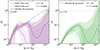 |
Fig. 4. Inferred halo occupation number for galaxies in the low-z and high-z DESI ELG samples. The solid (dashed) lines show the median of our model after marginalisation over all the SHAMe-SF parameters, whereas shaded regions (small and large circles) show the 1σ and 2σ regions for all galaxies (centrals). We compare the measured occupation distributions in our two DESI ELG mocks. DESI ELGs have similar mean halo masses as our mock DESI catalogues (DESI-TNG and DESI-SAM), but the abundance of satellites is systematically lower. We add as a reference the dotted grey line, indicating an abundance of ⟨N⟩ = 1. |
In the case of satellite ELGs, the average halo mass increases by ∼0.8 dex: log(Mh/h−1 M⊙) = 12.5 ± 0.2, and 12.5 ± 0.2, for the low and high-z samples. However, we find that satellite ELGs populate lower-mass haloes than in the DESI-TNG and DESI-SAM mock samples, where log(Mh/h−1 M⊙) = 12.9. SHAMe-SF places most of the satellites on masses in the interval log(Mh/h−1 M⊙)∈[11.8, 12.8]. For halo masses above 1013 h−1 M⊙, their median abundance drops, and we predict much larger uncertainties (almost two orders of magnitude for 1014 h−1 M⊙ in both redshift bins). This scatter between different realisations of the SHAMe-SF model is linked to the low contribution of haloes in these mass ranges to the clustering signal (see Contreras et al. 2013). We do not find the drop in the satellite abundance when comparing the low-z bin with the measurements on the mock DESI ELG samples.
5.2. Assembly bias
As observed in simulations, the halo spatial distribution depends on properties beyond halo mass (Sheth & Tormen 2004; Gao et al. 2005; Gao & White 2007; Wechsler et al. 2006; Faltenbacher & White 2010; Angulo et al. 2009; Mao et al. 2018). Since the evolution of subhaloes and galaxies is bound to that of their host haloes, this dependence (usually called assembly bias) will propagate to galaxies (Croton et al. 2007). The strength of the assembly bias signal varies depending on the hydrodynamic simulation (or SAM), number density, redshift or sample considered (Contreras et al. 2019, 2021a; Jiménez et al. 2021).
To quantify the amplitude of the assembly bias signal, we used the technique proposed by Croton et al. (2007), where the positions of haloes (including all their satellites) are shuffled among haloes within 0.1 dex bins in halo mass. We then estimated the assembly bias by comparing the shuffled and original correlation functions:
 (5)
(5)
We present the results of the inferred assembly bias signal in Fig. 5 for the low-z (top, purple) and high-z (bottom, green) DESI ELG samples. We find a non-negligible assembly bias signal for both redshift bins (between 10 and 20% for the low-z bin and ∼10% for the high-z bin). We obtain the same constraints shuffling using halo mass bins of 0.05 dex and 0.2 dex. In the case of the low-z bin, we also observe a scale dependence of the signal on large scales, compatible with the findings of Jiménez et al. (2021) for a SAM. The authors found different assembly bias signals for different number densities. Thus, we cannot assess the redshift evolution of assembly bias using these samples. Hadzhiyska et al. (2023a) point that part of this signal can originate from haloes misplaced as satellites by FoF + SUBFIND. To estimate this effect’s impact, we repeated the calculation only shuffling objects within r200c. We do not find deviations at large scales.
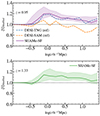 |
Fig. 5. Inferred magnitude of galaxy assembly bias in the low-z and high-z DESI ELG catalogues. We display the ratio of the correlation function in the best-fit SHAMe catalogue to a version where the position of haloes has been randomly shuffled among haloes of the same mass. Solid lines and shaded regions indicate the mean and 1σ region after marginalisation over all SHAMe parameters. We display the same quantity estimated in our mock DESI catalogues for comparison (DESI-TNG and DESI-SAM, dashed lines). At a fixed halo mass, DESI ELGs tend to be located preferentially in highly biased haloes, which is in qualitative agreement with the predictions of the TNG simulation. |
5.3. ELGs as satellites
Satellite galaxies dominate the clustering signal on small scales, where baryonic processes are also critical. Their evolution is more challenging to model than central galaxies due to the extensive variety of processes and interactions associated with satellites (gas stripping, strangulation, and ram pressure, among others).
Before analysing in depth what is happening to satellites, we measure how present they are in the sample in Sect. 5.3.1. We take a closer look at the radial phase distribution of these satellites in Sect. 5.3.2, and dedicate Sect. 5.3.3 to analyse the presence of angular anisotropies. We finish analysing central-satellite conformity in Sect. 5.3.4.
5.3.1. Satellite fractions
We next computed the satellite fractions inferred by the SHAMe-SF model. We have already verified that SHAMe-SF predicted reasonable satellite fractions compared to the DESI-TNG and DESI-SAM mock DESI ELG catalogues. We discuss further details in Appendix A.2.3. Since we are fitting galaxy clustering, labelling a galaxy as a central or a satellite does not change the given spatial distribution. In some cases, this labelling depends on the criteria of the (sub)halo finder: FoF + SUBFIND allows having satellite subhaloes beyond r200c, while in Rockstar (Behroozi et al. 2013) these objects would be considered centrals. This section uses both definitions to distinguish effects near the halo boundary and inside the virialised object.
We find that  % of the galaxies in the lowest redshift bin are satellites (or
  % when also considering as satellites outside r200c). These values are bracketed by the satellite fractions of the DESI-TNG and DESI-SAM mocks (see Table A.1), as pointed out in Sect. 4.2.
5.3.2. Radial phase-space distribution
In this section we analyse the number density profiles and radial velocities of satellite ELGs. The inferences from the SHAMe-SF model for DESI ELGs are presented in Fig. 6. We normalised the distances by the host halo r200c, and the infall velocity by the host v200 (virial velocity at r200c). We stacked the positions and velocities relative to r200c and v200 for satellite subhaloes with r > 0.1 h−1 Mpc (otherwise, their positions are not constrained by our fits) for all FoF haloes, and computed the distributions of r/r200c and vr/v200. We analysed the distributions by binning satellites in terms of their host halo mass. The aim is two-fold: (i) to analyse possible mass dependences of the profile, and (ii) to avoid normalisation issues originating from removing objects with r < 0.1 h−1 Mpc (since this scale is close to r200c for haloes with log(Mh [h−1 M⊙]) < 11.7).
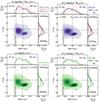 |
Fig. 6. Inferred phase-space distribution of ELG satellites in the low-z and high-z DESI samples for two halo mass bins for satellites with r > 0.1 h−1 Mpc (the minimum scale up to which we fitted the clustering). The contours mark the regions (from darker to lighter) containing 10%, 20%, …, 90%, and 99% of the total satellites. The fraction of all the satellites with r > 0.1 h−1 Mpc inside mass bins is indicated in each panel. The dashed brown line indicates where this division is located for each halo mass bin. Note that the axes are normalised in units of the host halo, r200 and v200. For comparison, we show the distribution of velocities and halo-centric distances as measured in our mock DESI catalogues (orange and blue lines for DESI-SAM and DESI-TNG, respectively), and for randomly selected dark matter particles (dotted lines). Most of the satellites are hosted by haloes with log(Mh [h−1 M⊙]) < 13. For radial velocities, the dashed line and the circled-hatched region represent the median and 1σ distribution for satellites with r < r200c. We can distinguish two populations, one infalling outside r200c with a negative infall velocity and a population mainly within the halo boundary with a distribution of radial velocities skewed towards negative values (also infalling). |
For the high-z and low-z samples in Fig. 6 (green and purple, respectively), we chose two halo mass bins, log(Mh [h−1 M⊙]) ∈ [12, 12.5], [12.5, 13]. We also analyse a higher-mass bin in Appendix B.1 (unlike the DESI-TNG and DESI-SAM samples, in DESI, we find that fewer than 2% of satellites are hosted in haloes with masses higher than 1013 h−1 M⊙).
Each diagram in Fig. 6 comprises three panels. The central larger panel shows the 2D distribution of distances and radial velocities of SHAMe-SF galaxies. The 1D projected distributions are shown on the upper and right panels. For comparison, we added the grey dotted line representing the dark matter profile from the simulation. We also include the mock DESI-TNG (blue) and DESI-SAM (orange) distributions for the same halo bins for the low-z sample. Appendix A.2.4 provides a detailed analysis of those samples.
We focused first on the ELGs within r200c (i.e. log(r/r200c) < 0). For all mass bins and redshifts, their velocity distribution leans towards more negative values (infalling) when compared to the randomly selected particles, as pointed out by Orsi & Angulo (2018). However, we do not find a significant preference towards the outskirts of the halo compared to the randomly chosen particles dark matter particles for the two lower-mass bins shown. In these mass bins, satellite ELGs seem closer to the halo centre than the underlying halo dark matter distribution.
However, the most interesting feature comes from scales beyond r200c. We can distinguish between two populations, a continuation of the profile inside r200c (with a distribution with infalling and outfalling velocities, but also tilted towards infalling) and a separately infalling population, clearly visible 2D histograms, where we observe two peaks in the distribution. As already analysed by Hadzhiyska et al. (2023a) for ELGs in the MillenniumTNG simulation (Hernández-Aguayo et al. 2023; Pakmor et al. 2023; Barrera et al. 2023; Kannan et al. 2023; Delgado et al. 2023; Ferlito et al. 2023; Contreras et al. 2023b), this globally infalling population may be a product of the FoF identifiers, which place two haloes on the same FoF object.
The relative importance of the infalling and orbiting populations for a given mass bin differs between the mock DESI samples. The quenching inside haloes of DESI-SAM is stronger than that of DESI-TNG, which causes ‘infalling ELGs’ to be dominant with respect to the orbiting ones. This is consistent with the findings of Orsi & Angulo (2018), but our DESI inference prefers a milder quenching inside haloes, similar to what we observe in TNG-DESI. Remarkably, this implies that ELG correlation functions can be used in the future to place constraints on ram pressure and quenching inside haloes.
5.3.3. Angular anisotropy
Even if the main focus of satellite modelling in HODs leans towards radial distributions, Hadzhiyska et al. (2023a) highlight the importance of anisotropy within haloes in their analysis of the MillenniumTNG simulation. The authors compare the satellite distributions to different HOD prescriptions, finding an improvement in the two-point correlation function when considering non-radially symmetric satellite distributions (in their case, parameterising the probability to assign a satellite to another satellite instead of always to the central subhalo).
Subhaloes are generally accreted via filaments, resulting in an excess distribution along the semi-major axis of haloes (Yang et al. 2006; Mezini et al. 2024). However, galaxies along the semi-major axis have been found to have a higher quenching fraction (Martín-Navarro et al. 2021; Karp et al. 2023), which would isotropise the distribution of blue galaxies. This difference also appears in the alignment for central red and blue galaxies on larger scales (e.g. Rodriguez et al. 2024).
As in the case of assembly bias, we only explored whether this effect is detectable in our catalogues. Following Hadzhiyska et al. (2023a), we kept the central-satellite distance, r, constant but randomly varied the angular distribution sampling new values of the spherical coordinates (ϕ, θ) and computed the ratio between the original and isotropised correlation functions. We present our inferences in Fig. 7 for the low-z (purple) and high-z (green) redshift bins. For comparison, we added the DESI-TNG and DESI-SAM results as dashed blue and orange lines for the low-z bin. We show the validation of anisotropy predictions for these mock DESI samples in Appendix A.2.5. The dashed line and circle-hatched region represent the median and 1σ intervals when only subhaloes within r200c are randomised. Solid lines display our results when considering all SUBFIND satellite subhaloes.
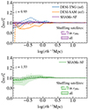 |
Fig. 7. Inferred magnitude of satellite anisotropy in the low-z and high-z DESI ELG catalogues. We display the ratio of the correlation function in the best-fit SHAMe catalogue to a version where the angular position of haloes has been randomly shuffled among each halo. Solid (dashed) lines and shaded (circle-hatched) regions indicate the mean and 1σ region after marginalisation over all SHAMe parameters when shuffling all satellites (only satellites within r200c). For comparison, we display the same quantity estimated in our mock DESI catalogues. |
Even if both redshift bins are consistent with an isotropic distribution on satellites, we find some deviations for the high-z bin (up to 5%). Anisotropy can be sourced by satellite pairs or the interaction between neighbouring haloes. The percentage haloes hosting more than one satellite is  % and
% and  % for the low-z and high-z bins, respectively. Pairs of satellites with small angular separations can also contribute to the higher signal on small scales observed in the data without necessarily adding central-satellite conformity.
5.3.4. Conformity
Conformity refers to correlations between the properties of nearby galaxies (e.g. Weinmann et al. 2006; Kauffmann et al. 2013; Vogelsberger et al. 2014; Hearin et al. 2015; Kauffmann 2015; Bray et al. 2016; Lacerna et al. 2018; Calderon et al. 2018). One of the most common examples is star-forming conformity: galaxies tend to be quenched around massive quenched centrals. Since ELGs are generally star-forming galaxies, we would expect them to be middle mass centrals (as discussed in Sect. 5.1), satellites near star-forming centrals or satellites in the outskirts of large and quenched galaxies. Due to the mass resolution of our simulation, our fits extend to scales of r > 0.1 h−1 Mpc. However, conformity has been detected observationally and in empirical models up to a few h−1 Mpc (e.g. Lacerna et al. 2022; Ayromlou et al. 2023). Since these scales fall within our range, we would expect to detect some amount of conformity in our fits. As discussed in Sect. 6.3.3, conformity is included in DESI models as a correlation between the probability of the central (sub)halo hosting satellite ELGs if the central galaxy is also an ELG (and thus there is central-satellite conformity). Even if the definition of satellite can change, the fraction of conformal haloes (close central-satellite pairs) is well constrained by the data on the amplitude of the auto-correlation on small scales, which cannot be explained using only satellite pairs (which would create a stronger angular anisotropy signal).
To analyse the central-satellite conformity in DESI’s ELGs, we computed the percentages of haloes in the sample that have only a central ELG (without ELG satellites), haloes with only satellites, and haloes with both centrals and satellites (thus, haloes exhibiting central-satellite conformity). The percentages and average halo masses are shown in Fig. 8 for the high-z and low-z DESI fit inferences (green and purple) and the DESI-TNG and DESI-SAM mock samples at z = 1 (blue and orange). We discuss the model validation using these mock samples in Appendix A.2.6.
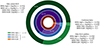 |
Fig. 8. Classification of the occupation of the host haloes of DESI high-z (green) and low-z (purple) samples, as well as the DESI-TNG and DESI-SAM mock samples at z ∼ 1 (blue and orange). We distinguish between haloes containing only a central ELG (top left), only ELG satellites (bottom right), and both ELG centrals and satellites (right, conformal haloes). We also provide the average halo masses in each case. All halo masses are expressed in h−1 M⊙ units. In all cases, the inference for DESI is bracketed between the DESI-TNG and DESI-SAM mock DESI catalogues. |
From all the selected haloes, only  % (
% ( %) of them host both ELG central and satellites in the low-z (high-z) sample. These quantities are bracketed by the values of our mock DESI ELG samples for the low-z bin (4.4% for DESI-TNG and 2.1% for DESI-SAM). SHAMe-SF predicts that these conformal haloes have lower average halo masses compared to non-conformal satellites
  (
( for the high-z sample).
We next explored whether this is caused by conformity. To do so, we shuffled satellites hosted by haloes within bins of 0.1 dex in halo mass. If the percentage of conformal haloes remains constant, then having an ELG central hosting ELG satellites would be similar within that halo mass bin. For the low-z and high-z bins, respectively, we obtain  % and
% and  %. Both percentages are reduced by more than half: even if the number of conformal ELG haloes is small in our sample, the type of central slightly conditions the presence of ELG satellites. This confirms the presence of central-satellite conformity in our ELG sample. The behaviour is similar for DESI-TNG and DESI-SAM mock DESI samples in the low-z bin, which is discussed in Appendix A.2.6.
6. Comparison with other analyses
In this section we compare our inferences from Sect. 5 with the findings of other analyses of DESI ELGs. Specifically, we explore the halo occupation number (Sect. 6.1), assembly bias (Sect. 6.2), and satellite fractions (Sect. 6.3.1), radial phase space (Sect. 6.3.2) and conformity (Sect. 6.3.3).
6.1. Halo occupation number
We began by comparing the average mass for centrals (or mass with the maximum central probability if the average halo mass is not provided) to get a first impression of how our results compare to other DESI ELG analyses. As shown in the right column of Fig. 9, our results are compatible within 1σ with all analyses except that of Yuan et al. (2023) when they include conformity and assembly bias simultaneously; the difference is mainly due to the inclusion of the assembly bias. In all cases, the average mass of haloes hosting centrals increases with redshift.
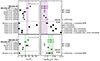 |
Fig. 9. Satellite fractions (left) and average centrals halo mass (right) for different analyses of DESI ELGs (Rocher et al. 2023; Yu et al. 2024; Prada et al. 2025; Gao et al. 2023, 2024; Yuan et al. 2023) for the two redshift intervals analysed in this work (0.8 < z < 1.1, purple; 1.1 < z < 1.6, green). The dashed black line separates HODs and SHAM within each redshift bin. The satellite fractions are computed for subhaloes as Nsatellites/(Ncentrals + Nsatellites). When the average halo mass for centrals is not provided, we add the halo mass with the highest probability (white symbols). In the cases from Yu et al. (2024) and Prada et al. (2025), average halo occupations are computed for 0.8 < z < 1.6. |
We can also compare the shape of the central occupation. For HODs, we can directly compare the parametrisation of the central occupation. Extended parametrisations for centrals in HODs are Gaussians (sometimes including decreasing power laws), error functions and log-normal distributions. All models predict a central occupation that increases to a peak probability and decreases afterwards except for Gao et al. (2023, 2024), which measure a second increase for higher halo masses on their SHAM. The width of the probability distribution also changes between models. Similar to this work, Rocher et al. (2023), Prada et al. (2025), and Yuan et al. (2023) find that the probability of finding central ELGs on haloes above 1013 h−1 Mpc solar masses is negligible (< 10−3; Yuan et al. 2023 when fitting auto-correlations that only include ELG conformity), whereas in Yu et al. (2024) and (2023, all other fits) have broader distributions.
6.2. Assembly bias
In the case of SHAM, assembly bias appears naturally (Chaves-Montero et al. 2016) and can be further tuned using explicit parameters (e.g. Contreras et al. 2021b). However, it must be included explicitly in HODs since their functional form depends only on halo mass (Hearin et al. 2016). Assembly bias can be introduced using many different secondary properties. The most extended ones are concentration and tracers of the small- or large-scale environment (Xu et al. 2021; Yuan et al. 2022b; Hadzhiyska et al. 2022; Beltz-Mohrmann et al. 2023)
In the case of DESI ELGs, Rocher et al. (2023) tested whether adding assembly bias through halo concentration, local halo density or local halo density anisotropy enhances the fit quality. Using the parametrisation described in Hadzhiyska et al. (2023b), the authors found little to no improvement after adding this effect. On the contrary, using the same parametrisation and shear as the secondary property, Yuan et al. (2023) find that including assembly bias in the vanilla HOD improves the fit to the ELG autocorrelation and its cross-correlation with luminous red galaxies. The authors leave the quantification of this effect for a future analysis. In our case, we measured an assembly bias signal larger than 5% (and non-compatible with 0 within the 1σ region) for both redshift bins.
6.3. ELGs as satellites
6.3.1. Satellite fractions
In this section we compare the satellite fraction inferred from SHAMe-SF fits to the predictions of DESI 1% analyses. All satellite fractions are summarised in the left column of Fig. 9. Since all of these works use Rockstar as their halo finder, the most direct comparison implies considering satellites only objects with r < r200c where r is the central-satellite distance, for which we find a satellite fraction of  %.
%.
The range of satellite fractions predicted by HODs varies drastically based on their assumptions. Yuan et al. (2023) found that 50% of ELGs were satellites when fitting only their projected correlation function and 30% when adding the cross-correlation with luminous red galaxies. The satellite fraction drops to 2% (10% when including cross-correlations) if conformity is included. This change is related to how conformity is modelled and where satellites are placed. Rocher et al. (2023) impose a strict conformity, linking the presence of ELG satellites to the presence of an ELG central. The authors predict satellite fractions of 2.6 ± 0.5% for the low-z sample and 3.5 ± 0.1%, similar to our fraction of conformal haloes (see Fig 8).
As for SHAM, Gao et al. (2023, 2024) fit scales comparable to Rocher et al. (2023) and Yuan et al. (2023) for cross-correlation between different stellar mass bins. They measure satellite fractions of 15.7% and 17.6% (when including conformity), which are more similar to our inferred values. Prada et al. (2025) and Yu et al. (2024) fit ELG clustering up to 4 h−1 Mpc, but find completely different satellite fractions: 17.9 ± 2.9% and  %, respectively. The main difference in the satellite fraction originates from how the subhaloes are chosen within the SHAM techniques (removing high Vpeak haloes in Yu et al. 2024, or using a Gaussian selection function in Prada et al.). The first term of our functional form (Eq. (1)) is more similar to the choice of Prada et al., which could explain the similarity in the satellite fractions. The satellites are down-sampled in both models regardless of their host halo mass.
6.3.2. Satellite radial phase space
Beyond modelling the number of satellites, halo-based models must include prescriptions for the position and velocities of satellites. In the case of subhalo-based models, the problem is reduced by adequately selecting the subhaloes that would host ELG satellites.
For satellite positions, HOD typical choices ranged from sampling from an assumed radial profile, like a likely a Navarro-Frenk-White (NFW) profile (Navarro et al. 1995), or randomly choosing the position of a dark matter particle within the halo. However, previous studies by Orsi & Angulo (2018) on a SAM point out that ELGs are typically located at the outskirts of haloes rather than following an NFW profile. This is included on HODs either using a modified NFW profile or adding additional probability functions to select the dark matter particles (Avila et al. 2020; Hadzhiyska et al. 2023a; Reyes-Peraza et al. 2024). For DESI-HODs, Rocher et al. (2023) find a significant improvement when sampling satellite positions from a scaled NFW profile with an additional exponential term for larger central-satellite distances. This extra term allows satellite placement beyond r200c; objects in this remote area would not be considered satellites by Rockstar. In the case of Yuan et al. (2023), the chosen method was randomly sampling from the dark matter particle distribution. Radial profiles inferred from our SHAMe-SF fits are more similar to the Rocher et al. (2023) parametrisation, and satellite ELGs only follow the dark matter distribution in the low-z sample in the mass range Mh > 1012.5 h−1 M⊙ (see Fig. 6 and Appendix B.1).
Likewise, it is necessary to assign velocities to the satellites. Typical approaches range from sampling from a given distribution (Hadzhiyska et al. 2023a), taking (or rescaling) the velocity of a dark matter particle (Rocher et al. 2023; Yuan et al. 2023), and sometimes adding an extra infall component term to a sampled velocity (Avila et al. 2020; Rocher et al. 2023). SHAMe-SF predicts velocity distributions tilted towards negative radial velocities for all mass bins, not following the underlying dark matter distribution (see Fig. 6).
6.3.3. Conformity
Some HODs and SHAM-based models applied to DESI’s data include conformity to improve the fitting to small scales (for r < 0.3 h−1 Mpc; Gao et al. 2024) or the transition between the one-halo and the two-halo term (Rocher et al. 2023; Yuan et al. 2023). Conformity is modelled as the probability of hosting ELG satellites depending on whether the central galaxy is also an ELG.
As discussed in Sect. 5.3.4, our fits predict that fewer than 5% of haloes host ELG centrals and ELG satellites simultaneously, and their typical masses are  and
and  , for the low-z high-z bins, respectively (see Fig. 8). Haloes hosting only ELG satellites have, on average, higher halo masses: log(Mh [h−1 M⊙]) ∼ 12.5. This tendency in the average halo masses would also appear in the Yuan et al. (2023) and Gao et al. (2024) analyses since the probabilities of conformal and non-conformal satellites have an offset in host halo masses. However, the number of conformal satellites (compared to satellites hosted by non-ELGs) is larger for Gao et al. (2024), as is shown in the halo occupation number they measure. For HODs that include conformity, the resultant occupation for ELG satellites will not be exactly the one parametrised by the power law. This is the case of Rocher et al. (2023) and Yuan et al. (2023). For the former, imposing a strict conformity would remove all satellites when a central is absent regardless of the ⟨Nsat⟩ probability given by the HOD. Conformity also affects the shape of the central HOD, which drives centrals to occupy higher halo masses to be able to host satellites. The percentage of conformal haloes predicted by SHAMe-SF for both redshift bins is similar to the satellite fractions from both HOD analyses when including conformity (see Fig. 9).
We also considered at the scenario presented in Favole et al. (2016) for g-selected ELGs at z ∼ 0.8, where they distinguish between ELG centrals (with masses around 1012 h−1 M⊙) and ELG satellites hosted by quiescent centrals whose halo masses were higher than 1013 h−1 M⊙. As mentioned, we find lower halo masses for ELGs in the lower-mass bin. Favole et al. (2016) also find that some of the most massive haloes would host more than one satellite, which happens for 1.3% of the haloes. These values align with our findings from Sect. 5.3.3 when analysing anisotropy, where we find  % and
% and  of haloes hosting more than one ELG satellite for the low-z and high-z samples, respectively. A combination of central-satellite conformity pairs and satellite-satellite pairs can source high clustering on smaller scales.
7. Summary and conclusions
We analysed the galaxy–halo connection of DESI ELGs between 0.8 < z < 1.1 (low-z) and 1.1 < z < 1.6. Our inferences were derived after fitting the galaxy clustering of these galaxies using SHAMe-SF, an extension to SHAM specially developed for star-forming galaxies. The SHAMe-SF model can reproduce the projected correlation function and the monopole and quadrupole of the correlation function in redshift space for both redshift bins between scales of 0.1 and 30 h−1 Mpc.
After fitting the DESI ELG clustering measurements (Sect. 4.2), we populated a gravity-only simulation using the best-fit parameters and inferred the galaxy–halo connection. Our findings for DESI ELGs can be summarised as follows:
-
ELGs inhabit haloes of average mass log(Mh [h−1 M⊙]) = 11.7 ± 0.1 (11.9 ± 0.1) when they are central and 12.5 ± 0.2 (12.6 ± 0.2) when they are satellites in the low-z (high-z) redshift bin, which match the values found by other DESI analyses (Sect. 6.1).
-
We detect a non-zero signal of assembly bias for the high-z (10%) and low-z (∼15%) samples. In the latter case, the signal is scale-dependent (Sect. 5.2).
-
In the low-z (high-z) sample, 34.0
 % (27.6
  %) of the galaxies are found to be satellites if using the FoF + SUBFIND central and satellite definitions, which includes galaxies outside r200c. This fraction decreases to 25.5
 % (19.5
 %) when only counting galaxies within r200c as satellites. Both estimations are generally higher than estimations of other studies with different galaxy–halo connection models (see Sects. 5.3.1 and 6.3.1).
 -
When analysing the phase space of satellite subhaloes, we find two distinct populations of satellites. The main population extends from the inner part of the halo out to beyond r200c. Their velocity distribution leans towards infalling. We also find a significant number of satellites outside r200c with negative radial velocities (infalling) in all halo mass bins. As discussed by Hadzhiyska et al. (2023a), they may be subhaloes misclassified by the halo finder (Sect. 5.3.2).
-
In both redshift bins, ELG satellites seem to be distributed almost isotropically within their haloes. We measure signatures of anisotropy in the galaxy clustering below 10% (Sect. 5.3.3).
-
Most satellites are hosted by non-ELG centrals (Sect. 5.3.4). Only
 % (
% ( %) of the haloes in the sample host both centrals and satellites. The typical halo masses of haloes that host both ELG centrals and satellites are lower than when they only host satellites.
The capability of the model to accurately reproduce these statistics was validated using DESI ELG samples from the TNG300-1 simulation and the L-Galaxies SAM run on TNG300-1-Dark merger trees (see Appendix A; Ayromlou et al. 2021). We show these tests and compare our mock samples with similar available catalogues in Appendix A.
We highlight the ability of the SHAMe-SF model to infer the radial phase-space distribution of satellites within different mass bins. Given the different predictions of TNG300 and L-Galaxies, we can use the SHAMe-SF model to provide further constraints on the satellite quenching and stripping modelling in hydrodynamic simulations and SAMs. After validating the SHAMe-SF model and confirming its capability to place constraints on the galaxy–halo connection, we aim to use it to obtain cosmological constraints.
Bias And Clustering Calculations Optimised.
z ∈ [1.49, 1.38, 1.31, 1.21, 1.14, 1.11, 0.98, 0.95, 0.89, 0.84].
Note that at r > 10 h−1 Mpc, we expect finite-box effects to impact the clustering measurements in the mocks. Therefore, we applied a correction estimated with simulations of two side lengths, as described in Appendix A.1.2.
Acknowledgments
We thank the anonymous referee for valuable and insightful comments. We also thank the DESI collaboration, particularly Antoine Rocher, for making the clustering measurements of DESI 1% available. SOM thanks the hospitality of Andrew Hearin, Georgios Zacharegkas and the rest of the CPAC Group at Argonne National Laboratory, where part of this work was carried out, and Mary Gerhardinger for useful discussions during that period. SOM also acknowledges Tamara Richardson for her insights on Halo Finders. SOM is funded by the Spanish Ministry of Science and Innovation under grant number PRE2020-095788. SC acknowledges the support of the ‘Juan de la Cierva Incorporacíon’ fellowship (IJC2020-045705-I). REA acknowledges support from project PID2021-128338NB-I00 from the Spanish Ministry of Science and support from the European Research Executive Agency HORIZON-MSCA-2021-SE-01 Research and Innovation Programme under the Marie Skłodowska-Curie grant agreement number 101086388 (LACEGAL). JCM, acknowledges support from the European Union’s Horizon Europe research and innovation programme (COSMO-LYA, grant agreement 101044612). IFAE is partially funded by the CERCA program of the Generalitat de Catalunya. The authors also acknowledge the computer resources at MareNostrum and the technical support provided by Barcelona Supercomputing Center (RES-AECT-2024-2-0022) Catalogues will be public upon publication of the paper in https://github.com/sortegamtnez/DESI_SHAMeSF.
References
- Alam, S., Peacock, J. A., Kraljic, K., Ross, A. J., & Comparat, J. 2020, MNRAS, 497, 581 [NASA ADS] [CrossRef] [Google Scholar]
- Angulo, R. E., & Pontzen, A. 2016, MNRAS, 462, L1 [NASA ADS] [CrossRef] [Google Scholar]
- Angulo, R. E., Lacey, C. G., Baugh, C. M., & Frenk, C. S. 2009, MNRAS, 399, 983 [CrossRef] [Google Scholar]
- Angulo, R. E., Springel, V., White, S. D. M., et al. 2012, MNRAS, 426, 2046 [NASA ADS] [CrossRef] [Google Scholar]
- Angulo, R. E., Zennaro, M., Contreras, S., et al. 2021, MNRAS, 507, 5869 [NASA ADS] [CrossRef] [Google Scholar]
- Aricò, G., Angulo, R. E., Hernández-Monteagudo, C., et al. 2020, MNRAS, 495, 4800 [Google Scholar]
- Aricò, G., Angulo, R. E., Contreras, S., et al. 2021, MNRAS, 506, 4070 [CrossRef] [Google Scholar]
- Avila, S., Gonzalez-Perez, V., Mohammad, F. G., et al. 2020, MNRAS, 499, 5486 [NASA ADS] [CrossRef] [Google Scholar]
- Ayromlou, M., Nelson, D., Yates, R. M., et al. 2021, MNRAS, 502, 1051 [NASA ADS] [CrossRef] [Google Scholar]
- Ayromlou, M., Kauffmann, G., Anand, A., & White, S. D. M. 2023, MNRAS, 519, 1913 [Google Scholar]
- Barrera, M., Springel, V., White, S. D. M., et al. 2023, MNRAS, 525, 6312 [NASA ADS] [CrossRef] [Google Scholar]
- Baugh, C. M. 2006, Rep. Progr. Phys., 69, 3101 [Google Scholar]
- Baugh, C. M., Lacey, C. G., Frenk, C. S., et al. 2005, MNRAS, 356, 1191 [Google Scholar]
- Behroozi, P. S., Wechsler, R. H., & Wu, H.-Y. 2013, ApJ, 762, 109 [NASA ADS] [CrossRef] [Google Scholar]
- Beltz-Mohrmann, G. D., Szewciw, A. O., Berlind, A. A., & Sinha, M. 2023, ApJ, 948, 100 [Google Scholar]
- Benson, A. J. 2010, Phys. Rep., 495, 33 [NASA ADS] [CrossRef] [Google Scholar]
- Benson, A. J., Cole, S., Frenk, C. S., Baugh, C. M., & Lacey, C. G. 2000, MNRAS, 311, 793 [NASA ADS] [CrossRef] [Google Scholar]
- Berlind, A. A., Weinberg, D. H., Benson, A. J., et al. 2003, ApJ, 593, 1 [NASA ADS] [CrossRef] [Google Scholar]
- Bower, R. G., Benson, A. J., Malbon, R., et al. 2006, MNRAS, 370, 645 [Google Scholar]
- Bray, A. D., Pillepich, A., Sales, L. V., et al. 2016, MNRAS, 455, 185 [NASA ADS] [CrossRef] [Google Scholar]
- Calderon, V. F., Berlind, A. A., & Sinha, M. 2018, MNRAS, 480, 2031 [Google Scholar]
- Chaves-Montero, J., Angulo, R. E., Schaye, J., et al. 2016, MNRAS, 460, 3100 [NASA ADS] [CrossRef] [Google Scholar]
- Chaves-Montero, J., Angulo, R. E., & Contreras, S. 2023, MNRAS, 521, 937 [Google Scholar]
- Cole, S., Lacey, C. G., Baugh, C. M., & Frenk, C. S. 2000, MNRAS, 319, 168 [Google Scholar]
- Conroy, C., Wechsler, R. H., & Kravtsov, A. V. 2006, ApJ, 647, 201 [Google Scholar]
- Contreras, S., & Zehavi, I. 2023, MNRAS, 525, 4257 [Google Scholar]
- Contreras, S., Baugh, C. M., Norberg, P., & Padilla, N. 2013, MNRAS, 432, 2717 [Google Scholar]
- Contreras, S., Baugh, C. M., Norberg, P., & Padilla, N. 2015, MNRAS, 452, 1861 [CrossRef] [Google Scholar]
- Contreras, S., Zehavi, I., Padilla, N., et al. 2019, MNRAS, 484, 1133 [NASA ADS] [CrossRef] [Google Scholar]
- Contreras, S., Angulo, R. E., & Zennaro, M. 2021a, MNRAS, 504, 5205 [CrossRef] [Google Scholar]
- Contreras, S., Angulo, R. E., & Zennaro, M. 2021b, MNRAS, 508, 175 [NASA ADS] [CrossRef] [Google Scholar]
- Contreras, S., Angulo, R. E., Chaves-Montero, J., White, S. D. M., & Aricò, G. 2023a, MNRAS, 520, 489 [Google Scholar]
- Contreras, S., Angulo, R. E., Springel, V., et al. 2023b, MNRAS, 524, 2489 [NASA ADS] [CrossRef] [Google Scholar]
- Contreras, S., Angulo, R. E., Chaves-Montero, J., et al. 2024, A&A, 690, A311 [NASA ADS] [CrossRef] [EDP Sciences] [Google Scholar]
- Croton, D. J., Gao, L., & White, S. D. M. 2007, MNRAS, 374, 1303 [Google Scholar]
- Cuesta-Lazaro, C., Nishimichi, T., Kobayashi, Y., et al. 2023, MNRAS, 523, 3219 [CrossRef] [Google Scholar]
- Davis, M., Efstathiou, G., Frenk, C. S., & White, S. D. M. 1985, ApJ, 292, 371 [Google Scholar]
- Delgado, A. M., Hadzhiyska, B., Bose, S., et al. 2023, MNRAS, 523, 5899 [CrossRef] [Google Scholar]
- DESI Collaboration (Aghamousa, A., et al.) 2016, arXiv e-prints [arXiv:1611.00036] [Google Scholar]
- DESI Collaboration (Adame, A. G., et al.) 2024a, AJ, 168, 58 [NASA ADS] [CrossRef] [Google Scholar]
- DESI Collaboration (Adame, A. G., et al.) 2024b, AJ, 167, 62 [NASA ADS] [CrossRef] [Google Scholar]
- Donnari, M., Pillepich, A., Nelson, D., et al. 2019, MNRAS, 485, 4817 [Google Scholar]
- Faltenbacher, A., & White, S. D. M. 2010, ApJ, 708, 469 [NASA ADS] [CrossRef] [Google Scholar]
- Favole, G., Comparat, J., Prada, F., et al. 2016, MNRAS, 461, 3421 [NASA ADS] [CrossRef] [Google Scholar]
- Favole, G., Montero-Dorta, A. D., Artale, M. C., et al. 2022, MNRAS, 509, 1614 [Google Scholar]
- Favole, G., Gonzalez-Perez, V., Ascasibar, Y., et al. 2024, A&A, 683, A46 [NASA ADS] [CrossRef] [EDP Sciences] [Google Scholar]
- Ferlito, F., Springel, V., Davies, C. T., et al. 2023, MNRAS, 524, 5591 [CrossRef] [Google Scholar]
- Foreman-Mackey, D., Hogg, D. W., Lang, D., & Goodman, J. 2013, PASP, 125, 306 [Google Scholar]
- Gao, L., & White, S. D. M. 2007, MNRAS, 377, L5 [NASA ADS] [CrossRef] [Google Scholar]
- Gao, L., Springel, V., & White, S. D. M. 2005, MNRAS, 363, L66 [NASA ADS] [CrossRef] [Google Scholar]
- Gao, H., Jing, Y. P., Zheng, Y., & Xu, K. 2022, ApJ, 928, 10 [Google Scholar]
- Gao, H., Jing, Y. P., Gui, S., et al. 2023, ApJ, 954, 207 [Google Scholar]
- Gao, H., Jing, Y. P., Xu, K., et al. 2024, ApJ, 961, 74 [Google Scholar]
- Garcia-Quintero, C., Mena-Fernández, J., Rocher, A., et al. 2025, JCAP, 2025, 132 [Google Scholar]
- Gonzalez-Perez, V., Comparat, J., Norberg, P., et al. 2018, MNRAS, 474, 4024 [NASA ADS] [CrossRef] [Google Scholar]
- Gonzalez-Perez, V., Cui, W., Contreras, S., et al. 2020, MNRAS, 498, 1852 [NASA ADS] [CrossRef] [Google Scholar]
- Griffin, A. J., Lacey, C. G., Gonzalez-Perez, V., et al. 2019, MNRAS, 487, 198 [NASA ADS] [CrossRef] [Google Scholar]
- Guo, Q., White, S., Boylan-Kolchin, M., et al. 2011, MNRAS, 413, 101 [Google Scholar]
- Guo, Q., White, S., Angulo, R. E., et al. 2013, MNRAS, 428, 1351 [NASA ADS] [CrossRef] [Google Scholar]
- Guo, H., Zheng, Z., Zehavi, I., et al. 2015, MNRAS, 446, 578 [NASA ADS] [CrossRef] [Google Scholar]
- Hadzhiyska, B., Tacchella, S., Bose, S., & Eisenstein, D. J. 2021, MNRAS, 502, 3599 [NASA ADS] [CrossRef] [Google Scholar]
- Hadzhiyska, B., Garrison, L. H., Eisenstein, D., & Bose, S. 2022, MNRAS, 509, 2194 [Google Scholar]
- Hadzhiyska, B., Hernquist, L., Eisenstein, D., et al. 2023a, MNRAS, 524, 2524 [NASA ADS] [CrossRef] [Google Scholar]
- Hadzhiyska, B., Eisenstein, D., Hernquist, L., et al. 2023b, MNRAS, 524, 2507 [NASA ADS] [CrossRef] [Google Scholar]
- Hearin, A. P., Watson, D. F., & van den Bosch, F. C. 2015, MNRAS, 452, 1958 [CrossRef] [Google Scholar]
- Hearin, A. P., Zentner, A. R., van den Bosch, F. C., Campbell, D., & Tollerud, E. 2016, MNRAS, 460, 2552 [NASA ADS] [CrossRef] [Google Scholar]
- Henriques, B. M. B., White, S. D. M., Thomas, P. A., et al. 2013, MNRAS, 431, 3373 [NASA ADS] [CrossRef] [Google Scholar]
- Henriques, B. M. B., White, S. D. M., Thomas, P. A., et al. 2015, MNRAS, 451, 2663 [Google Scholar]
- Henriques, B. M. B., Yates, R. M., Fu, J., et al. 2020, MNRAS, 491, 5795 [NASA ADS] [CrossRef] [Google Scholar]
- Hernández-Aguayo, C., Springel, V., Pakmor, R., et al. 2023, MNRAS, 524, 2556 [CrossRef] [Google Scholar]
- Jackson, T. M., Pasquali, A., Pacifici, C., et al. 2020, MNRAS, 497, 4262 [NASA ADS] [CrossRef] [Google Scholar]
- Jiménez, E., Contreras, S., Padilla, N., et al. 2019, MNRAS, 490, 3532 [CrossRef] [Google Scholar]
- Jiménez, E., Padilla, N., Contreras, S., et al. 2021, MNRAS, 506, 3155 [CrossRef] [Google Scholar]
- Jing, Y. P., Mo, H. J., & Börner, G. 1998, ApJ, 494, 1 [NASA ADS] [CrossRef] [Google Scholar]
- Kannan, R., Springel, V., Hernquist, L., et al. 2023, MNRAS, 524, 2594 [CrossRef] [Google Scholar]
- Karp, J. S. M., Lange, J. U., & Wechsler, R. H. 2023, ApJ, 949, L13 [NASA ADS] [CrossRef] [Google Scholar]
- Kauffmann, G. 2015, MNRAS, 454, 1840 [NASA ADS] [CrossRef] [Google Scholar]
- Kauffmann, G., Li, C., Zhang, W., & Weinmann, S. 2013, MNRAS, 430, 1447 [Google Scholar]
- Knebe, A., Knollmann, S. R., Muldrew, S. I., et al. 2011, MNRAS, 415, 2293 [Google Scholar]
- Lacerna, I., Contreras, S., González, R. E., Padilla, N., & Gonzalez-Perez, V. 2018, MNRAS, 475, 1177 [CrossRef] [Google Scholar]
- Lacerna, I., Rodriguez, F., Montero-Dorta, A. D., et al. 2022, MNRAS, 513, 2271 [NASA ADS] [CrossRef] [Google Scholar]
- Lacey, C. G., Baugh, C. M., Frenk, C. S., et al. 2016, MNRAS, 462, 3854 [Google Scholar]
- Lagos, C. D. P., Lacey, C. G., Baugh, C. M., Bower, R. G., & Benson, A. J. 2011, MNRAS, 416, 1566 [Google Scholar]
- Lagos, C. d. P., Lacey, C. G., & Baugh, C. M. 2013, MNRAS, 436, 1787 [NASA ADS] [CrossRef] [Google Scholar]
- Lan, T.-W., Prochaska, J. X., Moustakas, J., et al. 2024, ApJ, 977, 225 [Google Scholar]
- Lin, S., Tinker, J. L., Blanton, M. R., et al. 2023, MNRAS, 519, 4253 [CrossRef] [Google Scholar]
- Mao, Y.-Y., Zentner, A. R., & Wechsler, R. H. 2018, MNRAS, 474, 5143 [NASA ADS] [CrossRef] [Google Scholar]
- Marinacci, F., Vogelsberger, M., Pakmor, R., et al. 2018, MNRAS, 480, 5113 [NASA ADS] [Google Scholar]
- Martín-Navarro, I., Pillepich, A., Nelson, D., et al. 2021, Nature, 594, 187 [CrossRef] [Google Scholar]
- Mezini, L., Zentner, A. R., Wang, K., & Fielder, C. 2024, MNRAS, submitted [arXiv:2406.10150] [Google Scholar]
- Naiman, J. P., Pillepich, A., Springel, V., et al. 2018, MNRAS, 477, 1206 [Google Scholar]
- Navarro, J. F., Frenk, C. S., & White, S. D. M. 1995, MNRAS, 275, 720 [NASA ADS] [CrossRef] [Google Scholar]
- Nelson, D., Pillepich, A., Springel, V., et al. 2018, MNRAS, 475, 624 [Google Scholar]
- Norberg, P., Baugh, C. M., Gaztanaga, E., & Croton, D. J. 2009, MNRAS, 396, 19 [NASA ADS] [CrossRef] [Google Scholar]
- Nusser, A., Yepes, G., & Branchini, E. 2020, ApJ, 905, 47 [Google Scholar]
- Onions, J., Knebe, A., Pearce, F. R., et al. 2012, MNRAS, 423, 1200 [Google Scholar]
- Orsi, Á. A., & Angulo, R. E. 2018, MNRAS, 475, 2530 [NASA ADS] [CrossRef] [Google Scholar]
- Ortega-Martinez, S., Contreras, S., & Angulo, R. 2024, A&A, 689, A66 [NASA ADS] [CrossRef] [EDP Sciences] [Google Scholar]
- Pakmor, R., Springel, V., Coles, J. P., et al. 2023, MNRAS, 524, 2539 [NASA ADS] [CrossRef] [Google Scholar]
- Peacock, J. A., & Smith, R. E. 2000, MNRAS, 318, 1144 [Google Scholar]
- Pellejero Ibañez, M., Angulo, R. E., Zennaro, M., et al. 2023, MNRAS, 520, 3725 [Google Scholar]
- Pillepich, A., Nelson, D., Hernquist, L., et al. 2018, MNRAS, 475, 648 [Google Scholar]
- Planck Collaboration XIII. 2016, A&A, 594, A13 [NASA ADS] [CrossRef] [EDP Sciences] [Google Scholar]
- Popesso, P., Biviano, A., Finoguenov, A., et al. 2015, A&A, 579, A132 [NASA ADS] [CrossRef] [EDP Sciences] [Google Scholar]
- Prada, F., Ereza, J., Smith, A., et al. 2025, A&A, in press https://doi.org/10.1051/0004-6361/202451022 [Google Scholar]
- Pujol, A., Gaztañaga, E., Giocoli, C., et al. 2014, MNRAS, 438, 3205 [Google Scholar]
- Raichoor, A., Comparat, J., Delubac, T., et al. 2016, A&A, 585, A50 [NASA ADS] [CrossRef] [EDP Sciences] [Google Scholar]
- Raichoor, A., Eisenstein, D. J., Karim, T., et al. 2020, Res. Notes Am. Astron. Soc., 4, 180 [Google Scholar]
- Raichoor, A., Moustakas, J., Newman, J. A., et al. 2023, AJ, 165, 126 [NASA ADS] [CrossRef] [Google Scholar]
- Reyes-Peraza, G., Avila, S., Gonzalez-Perez, V., et al. 2024, MNRAS, 529, 3877 [NASA ADS] [CrossRef] [Google Scholar]
- Rocher, A., Ruhlmann-Kleider, V., Burtin, E., et al. 2023, JCAP, 2023, 016 [CrossRef] [Google Scholar]
- Rodriguez, F., Merchán, M., & Artale, M. C. 2024, A&A, 688, A40 [NASA ADS] [CrossRef] [EDP Sciences] [Google Scholar]
- Shankar, F., Lapi, A., Salucci, P., De Zotti, G., & Danese, L. 2006, ApJ, 643, 14 [NASA ADS] [CrossRef] [Google Scholar]
- Sheth, R. K., & Tormen, G. 2004, MNRAS, 350, 1385 [NASA ADS] [CrossRef] [Google Scholar]
- Sinha, M. 2016, https://doi.org/10.5281/zenodo.55161 [Google Scholar]
- Sinha, M., & Garrison, L. 2017, Astrophysics Source Code Library [record ascl:1703.003] [Google Scholar]
- Springel, V., White, S. D. M., Tormen, G., & Kauffmann, G. 2001, MNRAS, 328, 726 [Google Scholar]
- Springel, V., White, S. D. M., Jenkins, A., et al. 2005, Nature, 435, 629 [Google Scholar]
- Springel, V., Pakmor, R., Pillepich, A., et al. 2018, MNRAS, 475, 676 [Google Scholar]
- Trujillo-Gomez, S., Klypin, A., Primack, J., & Romanowsky, A. J. 2011, ApJ, 742, 16 [Google Scholar]
- Vale, A., & Ostriker, J. P. 2006, MNRAS, 371, 1173 [NASA ADS] [CrossRef] [Google Scholar]
- Vogelsberger, M., Genel, S., Springel, V., et al. 2014, MNRAS, 444, 1518 [Google Scholar]
- Vos-Ginés, B., Avila, S., Gonzalez-Perez, V., & Yepes, G. 2024, MNRAS, 530, 3458 [Google Scholar]
- Weaver, J. R., Kauffmann, O. B., Ilbert, O., et al. 2022, ApJS, 258, 11 [NASA ADS] [CrossRef] [Google Scholar]
- Wechsler, R. H., & Tinker, J. L. 2018, ARA&A, 56, 435 [NASA ADS] [CrossRef] [Google Scholar]
- Wechsler, R. H., Zentner, A. R., Bullock, J. S., Kravtsov, A. V., & Allgood, B. 2006, ApJ, 652, 71 [NASA ADS] [CrossRef] [Google Scholar]
- Weinmann, S. M., van den Bosch, F. C., Yang, X., & Mo, H. J. 2006, MNRAS, 366, 2 [NASA ADS] [CrossRef] [Google Scholar]
- Xu, X., Zehavi, I., & Contreras, S. 2021, MNRAS, 502, 3242 [NASA ADS] [CrossRef] [Google Scholar]
- Yang, X., van den Bosch, F. C., Mo, H. J., et al. 2006, MNRAS, 369, 1293 [NASA ADS] [CrossRef] [Google Scholar]
- Yu, J., Zhao, C., Gonzalez-Perez, V., et al. 2024, MNRAS, 527, 6950 [Google Scholar]
- Yuan, S., Hadzhiyska, B., Bose, S., & Eisenstein, D. J. 2022a, MNRAS, 512, 5793 [NASA ADS] [CrossRef] [Google Scholar]
- Yuan, S., Garrison, L. H., Hadzhiyska, B., Bose, S., & Eisenstein, D. J. 2022b, MNRAS, 510, 3301 [NASA ADS] [CrossRef] [Google Scholar]
- Yuan, S., Wechsler, R. H., Wang, Y., et al. 2023, MNRAS, submitted [arXiv:2310.09329] [Google Scholar]
- Zehavi, I., Blanton, M. R., Frieman, J. A., et al. 2002, ApJ, 571, 172 [NASA ADS] [CrossRef] [Google Scholar]
- Zehavi, I., Zheng, Z., Weinberg, D. H., et al. 2011, ApJ, 736, 59 [NASA ADS] [CrossRef] [Google Scholar]
- Zennaro, M., Angulo, R. E., Pellejero-Ibáñez, M., et al. 2023, MNRAS, 524, 2407 [Google Scholar]
- Zheng, Z., Berlind, A. A., Weinberg, D. H., et al. 2005, ApJ, 633, 791 [NASA ADS] [CrossRef] [Google Scholar]
- Zheng, Z., Coil, A. L., & Zehavi, I. 2007, ApJ, 667, 760 [Google Scholar]
Appendix A: SHAMe-SF model validation
Hydrodynamic simulations and SAMs provide a unique opportunity to test empirical models such as HODs and SHAM against different plausible realisations of the Universe before applying them to observational data. Since both hydrodynamic simulations and SAMs contain all the information on the galaxy–halo connection, we can use them to validate whether the assumptions made on SHAM and HODs hold after fitting the galaxy clustering. We can also analyse different predictions of each model that are not constrained directly by the model parameters, such as galaxy assembly bias or the satellite distribution, comparing them with the ‘ground truth’ of the simulation.
In Ortega-Martinez et al. (2024), we verified that the SHAMe-SF model could reproduce the galaxy clustering of samples selected by SFR or colour cuts (without considering incompleteness). However, the selection criteria for ELGs are more complex. Through this appendix, we validate the behaviour of the SHAMe-SF model when applied to mock DESI ELG samples (see Sect. 2.2.2 for the selection criteria) and specifically how accurately we can predict their galaxy–(sub)halo connection after fitting the clustering. We assumed that the redshift bin (0.8 < z < 1.1) is narrow enough to exclude redshift evolution, and chose our galaxies at redshift z = 1 from TNG300-1 and L-Galaxies. After applying the stellar mass and SFR cuts, the resultant number densities were  (DESI-TNG) and
  (DESI-SAM).
We dedicate Appendix A.1 to the galaxy clustering fits, while Appendix A.2 includes all the validation of the galaxy–(sub)halo connection inferences.
A.1. Galaxy clustering
Before venturing into fitting DESI ELG’s galaxy clustering, we ensured that SHAMe-SF can reproduce the galaxy clustering of both mock DESI samples. Through this section, we present two auxiliary simulations used to estimate the covariance matrices (Appendix A.1.1), discuss the volume correction introduced for large scales, given the difference in size between TNG300 (Appendix A.1.2) and the simulation used to create the emulator (and DESI’s survey effective volume), the covariance matrices (Appendix A.1.3), and finally present our fits for DESI-TNG and DESI-SAM mock ELG samples (Appendix A.1.4).
A.1.1. Auxiliary simulations
In addition to the simulations used to create the emulator and the posterior predictive distributions described in Sect. 3.2, we used two gravity-only simulations with lower resolution: TNG-mimic and LTNG (Large TNG).
The TNG-mimic simulation has the same volume and initial conditions as TNG300-1-Dark, but employs only 6253 particles (equivalent resolution to TNG300-3-Dark). LTNG also has Gaussian initial conditions and resolution, but its volume is 27 times larger. Both simulations were run with an updated version the L-Gadget3 code (Angulo et al. 2012; Springel et al. 2005) used on the other BACCO simulations.
A.1.2. Box-size correction
Our DESI ELG mocks were built using TNG300-1, a relatively small simulation box, L = 205 h−1Mpc. This implies that the correlation functions on large scales are systematically underestimated due to the lack of long wavelength modes. To correct for this, we proceeded as follows.
First, we found the set of SHAMe-SF parameters that best fit the clustering of either DESI-TNG or DESI-SAM mocks as described in Sect. 4 for the monopole and the quadrupole (since we are using πmax = 40h−1Mpc on wp). We only considered separations below r = 7 h−1Mpc to ensure the finite box size does not affect the measurements. Then, we used those parameters to populate TNG-mimic and our 1 h−1Gpc simulation, described in Sect. 3.2. We then corrected the clustering measurements as
 (A.1)
(A.1)
where  and the subscripts 1000 and 200 refer to quantities computed in TNG-mimic and the 1000 h−1Mpc simulations, respectively. In Fig. A.1 we show the clustering measurements before (dashed) and after (points with error bars) this correction (blue and orange for DESI-TNG and DESI-SAM, respectively).
A.1.3. Covariance matrices
Given the small volume of TNG300 and the low number density of our target sample, it is not possible to have a robust estimator of the covariance matrix, especially the non-diagonal terms. We can surpass this using a larger simulation to compute the correlation matrix, and then re-scale it using the diagonal term from 33 jackknife samples (Zehavi et al. 2002; Norberg et al. 2009) directly over the mock DESI samples.
Using the method described in Sect. 4, we obtain a preliminary fit using SHAMe-SF for each of the mock DESI catalogues using the diagonal Cv. Using the best-fit parameters, we populate LTNG (Appendix A.1.1), compute the correlation matrix using 93 jackknife divisions, and re-scale them using the previously computed diagonal elements. As in the case of DESI fits, we added to the diagonal the contribution of the emulator error.
A.1.4. DESI-TNG and DESI-SAM clustering
Since clustering statistics are invariant under random down-samplings to the data, we used the non-down-sampled measurements of wp and ξℓ = 0, 2. We proceeded as described in Sect. 4 to fit the galaxy clustering of the DESI-TNG and DESI-SAM mock samples. The best-fit results are shown in Fig. A.1 for DESI-TNG (blue) and DESI-SAM (orange). We include the value of the reduced χ2 in the right panel for each sample. SHAMe-SF is able to reproduce the galaxy clustering in both cases.
Even if the samples were defined using similar selection criteria, their behaviours differ on both large and small scales. Given the difference on the small scales, we expect DESI-SAM to have fewer satellites than DESI-TNG. Furthermore, the upturn in the projected correlation function of DESI-TNG for scales below 0.3h−1Mpc is similar to that found for DESI’s ELGs, appearing at even smaller scales, which is not found in DESI-SAM. Two possible sources are central-satellite pairs (that would manifest on the satellite distributions of conformal galaxies) or satellite-satellite pairs (producing angular anisotropies in the satellite distribution), both related to the satellite fraction of the sample.
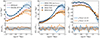 |
Fig. A.1. Projected correlation function (wp), and the monopole and quadrupole of the DESI-TNG (blue error bars) and DESI-SAM (orange error bars) ELGs at z = 1 defined using the selection criteria explained in Sect. 2.2.2. The solid lines show the corresponding best fit using the SHAMe-SF model. Lower panel: Relative difference between the fits and the data normalised by the uncertainty on the measurement, with the grey shaded region indicating 1σ. The dashed blue and orange lines show the measurements before the box-size correction (b.s.c.) introduced in Appendix A.1.2. The dashed purple line displays the measurements for DESI ELGs at 0.8 < z < 1.1 (Rocher et al. 2023) fitted in Fig. 2. |
A.2. DESI-TNG(SAM) galaxy–subhalo connection
As described in Sect. 5, we computed the posterior predictive distributions for assembly bias, halo occupation number, and satellite statistics. We repopulated the Planck 512h−1Mpc simulation (Sect. 3.2) using 100 random elements of the MCMC chains. In this case, we compared them with the true value computed from DESI-TNG and DESI-SAM mock galaxy samples. We averaged the measurements over ten random down-samplings with the same number density of the DESI low-z sample ( ).
).
We compared our inferences with DESI ELG mocks from other works using different selection criteria in simulations and SAMs. Specifically, we compared with samples built using DESI colour selection on TNG300 from (Hadzhiyska et al. 2021, z = 0.8 and z = 1) and Yuan et al. (2022a, z ∼ 0.8), M*-sSFR-selected samples from the MillenniumTNG simulation at z = 1 (for a number density two times larger; Hadzhiyska et al. 2023b,a), and with the colour and [OII]-selected sample from Gonzalez-Perez et al. (2018) and Gonzalez-Perez et al. (2020) in the GALFORM SAM4.
All the quantities computed (for the DESI mock samples and the SHAMe-SF predictions) can be found in Table A.1. We verified that the inferences were consistent before and after applying the box-size correction.
A.2.1. Assembly bias
To test whether SHAMe-SF can reproduce the dependence of galaxy clustering on properties beyond halo mass of the mock DESI samples, we followed the procedure described in Sect. 5.2. We show the results for DESI-TNG and DESI-SAM in Fig. A.2. In each case, the prediction of the hydrodynamic simulation (or SAM) is shown with the solid black line. The error bars indicate the 1σ deviation over ten realisations. The shaded regions in blue (for DESI-TNG) and orange (for DESI-SAM) regions show the 1σ SHAMe-SF predictions after fitting the galaxy clustering.
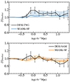 |
Fig. A.2. Same as Fig. 5 but for DESI-TNG (top, blue) and DESI-SAM (bottom, orange) mock DESI samples. The black error bars mark the measurements from the simulation and SAM, while the shaded regions indicate the predictions from the SHAMe-SF model. We can reproduce the assembly bias signal in both cases. Note the scale dependence of DESI-SAM. |
We find different assembly bias signatures in the two samples and a good agreement between the simulation or SAM and the prediction of SHAMe-SF. This shows the potential of SHAMe-SF to constrain galaxy assembly bias from galaxy clustering.
For DESI-TNG, the signal does not show a clear scale dependence and has a value of around 10%. For DESI-SAM, we measured an assembly bias closer to 0, but it shows scale dependence between ∼5% leaning towards negative values for larger scales. These values are in agreement with other previous works on TNG (Hadzhiyska et al. 2021), MillenniumTNG (Hadzhiyska et al. 2023b) and SAMs Gonzalez-Perez et al. (2020).
A.2.2. HOD
The halo occupation numbers of the mock DESI samples and the inferences from the SHAMe-SF model are shown in Fig. A.3. The reference distributions on DESI-TNG and DESI-SAM are shown with the black error bars with solid lines for all galaxies, and dashed lines for centrals. In this case, we plot the 1σ and 2σ regions for SHAMe-SF predictions (shaded region for all galaxies, big and small circle-hatched region for centrals).
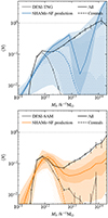 |
Fig. A.3. Same as Fig. 4, but for the inferred halo occupation number for DESI-TNG (top, blue) and DESI-SAM (bottom, orange) mock DESI samples. Measurements from the simulation and SAM are shown in black. The main difference between the two samples is the satellite probability. |
SHAMe-SF predicts a broader distribution for central galaxies in DESI-TNG. A similar effect was observed by Zehavi et al. (2011) and Contreras et al. (2024), where the low-mass transition is not fully constrained by galaxy clustering. The bump in the total distribution at high halo masses (dominated by satellite occupancy) is produced by the implementation of the quenching mechanism in SHAMe-SF. We underpredict the number of satellites in haloes with Mh > 1013 h−1M⊙. Of all the satellites in the sample, 16% are hosted by those haloes, while we predict 4+8−1% (see Table A.1). The behaviour of the HOD for satellites is similar to what was found by Gonzalez-Perez et al. (2018), Hadzhiyska et al. (2021), Yuan et al. (2022a), and Hadzhiyska et al. (2023a). For DESI-SAM, the model delivers accurate predictions for centrals and satellites hosted by haloes with masses below 1013 h−1M⊙, but again underestimates the number of satellites and centrals for higher halo masses. This does not seem to affect the (normalised) predictions of the radial distance and velocity distributions.
Beyond these differences, SHAMe-SF recovers the mean halo masses of centrals for DESI-TNG (log(Mh /h−1M⊙) = 12.1 ) and TNG-SAM (log(Mh/h−1M⊙) = 12.0
 ). For satellites, we recover the average halo mass for DESI-TNG (log(Mh/h−1M⊙) = 13.0
 ), but, as expected from the shape of the halo occupation number, we under-predict by 0.2 dex average halo mass for DESI-SAM (log(Mh/h−1M⊙) = 12.6
 from SHAMe-SF, log(Mh/h−1M⊙) = 12.9 as measured in L-Galaxies).
A.2.3. Satellite fractions
Even if the central or satellite classification depends on the criteria used to define what a satellite is (and this definition does not impact galaxy clustering), it is a necessary check to assess the significance of the rest of the predictions in this section. If the model significantly fails to reproduce the number of satellites, all future claims about their distribution will not be accurate.
We anticipated that the satellite fraction would be different between our mock DESI samples given the differences in the one-halo term (see the discussion of galaxy clustering in Appendix A.1.4). 36.9% of the galaxies in the DESI-TNG mock sample are satellites, while we find only 14.5% in DESI-SAM. The satellite fractions of both mock samples and SHAMe-SF’s inferences are shown in the top rows of Table A.1. SHAMe-SF is able to recover the sample fractions within the error bars for DESI-TNG (for both satellite definitions, FoF+SUBFIND and within r200c) and within the halo boundary for DESI-SAM. SHAMe-SF underpredicts by 3% the number of satellites considering objects beyond r200c. The effect of this manifests when looking at satellite anisotropy in Appendix A.2.5. The satellite fractions predicted by other works also show significant deviations, ranging between 4% (Gonzalez-Perez et al. 2020) and 36% (Hadzhiyska et al. 2023a).
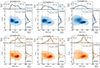 |
Fig. A.4. Same as Fig. 6 but for the phase space of the central–satellite distance and the radial velocity of three bins in halo mass. We only include satellites with r > rmin fit. The measurements from the mock DESI catalogues are shown in black in the projected histograms, while the shaded regions mark our posterior predictive distributions. There is no difference between mass bins in DESI-SAM. For the highest-mass bin in the DESI-TNG sample, the satellite density profile closely follows the distribution of randomly selected particles. This is not the case for velocities. |
A.2.4. Satellite phase-space distribution
Satellite phase space is the main modelling challenge for HODs. We analysed whether the inferences of SHAMe-SF for the mock DESI ELG samples are realistic. In Fig. A.4 we show the equivalent of Fig. 6 for the same mass bins, adding the comparison with the measurements on DESI-TNG/DESI-SAM on the projected histograms (black lines). We also include the fraction of satellites with r > rmin fit in each mass bin predicted by SHAMe-SF and measured in the simulation/SAM (see also Table A.1). SHAMe-SF reproduces the central-satellite distance and velocity distributions for the three mass bins, only finding small differences in the velocity distribution inside r200c for DESI-TNG.
Looking at the 2D distribution, we find the same bimodality we pointed out for DESI galaxies (infalling and virialised subhaloes). We highlight that satellites in the high-mass bin of TNG300 closely follow the randomly selected dark matter distribution (equivalent to an NFW profile). The behaviour of DESI-SAM satellites is more similar between the different mass bins, where most satellites are infalling and outside r200c. This is related to the implementation of the quenching mechanisms in the L-Galaxies version from Henriques et al. (2015), where tidal stripping only acts within r200c (for more details on the difference between DESI-TNG and DESI-SAM quenching mechanisms, see Ayromlou et al. 2021). Overall, we are confident when predicting the radial distributions for DESI ELGs presented in Sect. 5.3.2.
We can compare our distance profiles with the distributions from Yuan et al. (2022a) and Hadzhiyska et al. (2023a). Yuan et al. (2022a) find a similar mass dependence for TNG300, with a bimodality inside and outside r200c that vanishes for halo masses larger than 1013 h−1M⊙, where the distribution of ELG satellites coincides with the halo mass distribution. However, in the case of Hadzhiyska et al. (2023a), the bimodality can be found for all halo masses. The distribution of the radial velocities is similar to our DESI-TNG sample, leaning towards negative velocities with a peak associated with the infalling population outside r200c.
A.2.5. Satellite angular anisotropy
Here we validate our predictions from Sect. 5.3.3 when altering the angular distributions of satellites. We followed the same procedure as Hadzhiyska et al. (2023a) and kept the central-satellite distance constant while randomly varying the angular positions of satellites within each halo. We show our results in Fig. A.5 when shuffling satellites within r200c (dashed line, circle-hatched region) and all satellites (solid line and shaded region). For both shufflings, DESI-TNG presents some scale-dependent effect of anisotropy that does not appear for the DESI-SAM. The signal’s shape is similar to Hadzhiyska et al. (2023a)’s findings when comparing the isotropic HOD with the right satellite distribution, but we find a smaller amplitude. The difference in the signal between DESI-TNG and DESI-SAM comes from the implementation of AGN feedback (anisotropic for DESI-TNG, uniform in the SAM). SHAMe-SF predicts a smaller amplitude for the small-scale anisotropy when shuffling all the satellites in DESI-SAM. This is sourced by the difference in the number of satellites outside r200c measured in the SAM and predicted by SHAMe-SF. When shuffling satellites within r200c, we do not measure any anisotropy. We attribute this to the lack of satellite pairs measured in both the mock DESI sample and the SHAMe-SF model prediction (see Table A.1).
A.2.6. Central-satellite conformity
While discussing central-satellite conformity in Sect. 5.3.4, we found that only a small percentage of haloes hosted both central and satellite ELGs. Even if conformity is not implemented explicitly in SHAMe-SF, it successfully recovers the percentage of conformal haloes for both DESI-TNG (63.6%) and DESI-SAM (85.0%) mock DESI ELG samples. The percentages and average halo masses of haloes hosting only centrals, only satellites and centrals and satellites (conformal) are summarised in Fig. A.6 and Table A.1 for DESI-TNG (blue) and DESI-SAM (orange) mock samples. Both quantities are accurately reproduced by SHAMe-SF.
The average masses of haloes hosting only centrals (log(Mh/h−1M⊙)∼11.9), only satellites (log(Mh/h−1M⊙)∼13), or both (log(Mh/h−1M⊙)∼12.2) in the two mock DESI ELG samples are very similar. Thus, the difference in the fraction of conformal haloes is due to the difference in the satellite fraction between the samples and not necessarily to the physical processes that give rise to conformity.
To elucidate whether the satellite placement was casual or there was a correlation with the type of central, we repeated the shuffling exercise described in Sect. 5.3.4. With the SHAMe-SF model (reference) we find  % (
% ( %) and
  % (
% ( %). Thus, we find conformity for the DESI-TNG sample, but we cannot asses whether it is only a statistical effect in DESI-SAM given the discrepancy between our estimation and the measured percentage.
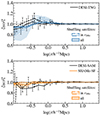 |
Fig. A.5. Quantification of the effect of the angular satellite distribution on the galaxy clustering (similar to Fig. 7). We mark the measurements from the mock DESI catalogues using the black lines: solid when all the satellites are shuffled, dashed when only the positions of satellites within r200c are changed. |
 |
Fig. A.6. Comparison between the host haloes of ELGs in the mock DESI samples (dimmer oranges, inner circles for each colour) and the predictions from SHAMe-SF. As in Fig. 8, we distinguish between haloes with only a central ELG, haloes with only ELG satellites, and haloes with both (conformal), and provide the average measured halo masses and those predicted by the model. The uncertainties on the percentage can be found in Table A.1. Most ELGs are centrals without other ELG satellites. Haloes that host both central and satellite ELGs have lower masses than those only containing satellites. |
Comparison between the measured and inferred (SHAMe-SF) galaxy–(halo) connection for DESI-TNG and DESI-SAM.
Appendix B: DESI posteriors
B.1. Satellites in other halo mass bins
In Sect. 5.3.2 we analyse the phase space of host haloes with 12 < log(Mhh−1M⊙) < 13. We dedicate this appendix to satellites hosted by higher- and lower-mass haloes. Table B.1 summarises the fraction of satellites with r > rmin fit in each mass bin.
In Fig. B.1 we show the central-satellite distance and the radial velocities for the highest-mass bin in halo mass, Mh ∈ [1013, 1014] h−1M⊙. The SHAMe-SF model predicts that only 1% of all satellites are in this mass bin, fewer than in the DESI-TNG and DESI-SAM mock samples. As for the other mass bins, we distinguish two populations: a virialised population (inside and outside r200c) with a mostly infalling distribution of velocities and an infalling population outside r200c. In this mass bin, the latter dominates, similar to the case of DESI-SAM and unlike DESI-TNG. Since the radial position distribution is dominated by the infalling term, we cannot assess whether the virialised component follows the dark matter, as in the case of DESI-TNG.
For haloes with log(Mh/h−1M⊙) < 12, the value of r200c is very close to the minimum scales in the fits (rmin fit). As in the case of other mass bins, we find infalling satellites outside of r200c, but we cannot characterise the satellite distribution within the halo boundary.
Distribution of satellite haloes in terms of host halo mass. All halo masses are expressed in terms of h−1M⊙.
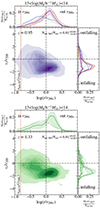 |
Fig. B.1. Same as Fig. 6 but for satellites on haloes with Mh ∈ [1013, 1014] h−1M⊙. For these halo masses, the infalling population dominates for both redshift bins. |
B.2. All posteriors
We discuss in Sect. 4.2 the meaning of constraining some of the SHAMe-SF parameters when fitting the clustering. The full posterior distributions are shown in Fig. B.2. We used the same ranges for the parameters on the emulator training and the priors. β, γ, Δγ, α0, and αexp control the amplitude of the score used to rank-order the subhaloes before applying the cut in number density. Fixing the value of one of these parameters can be reabsorbed by the others to produce the same clustering signal. This is also true for larger values of σ. Values of σ very close to zero would imply that the secondary dependence on concentration (parametrised by both fk) is not important, which seems to be discarded by the posterior.
 |
Fig. B.2. Marginalised 1σ constraints on all SHAMe-SF parameters, obtained from fitting the clustering of DESI ELGs at z = 0.95 (purple) and 1.33 (green). |
All Tables
Comparison between the measured and inferred (SHAMe-SF) galaxy–(halo) connection for DESI-TNG and DESI-SAM.
Distribution of satellite haloes in terms of host halo mass. All halo masses are expressed in terms of h−1M⊙.
All Figures
|
Fig. 1. Distribution of stellar masses (M*) and SFRs for galaxies at z = 1 as predicted by the TNG300 hydrodynamic simulation (‘DESI-TNG’, left panel) and by the L-Galaxies semi-analytic galaxy formation model (‘DESI-SAM’, right panel). Our mock DESI samples are defined by selection criteria for M*, SFRs, and the main sequence (similar to a cut in the sSFR), as indicated by solid lines (see Fig. 5 of Yuan et al. 2023 for a crossmatch between observed DESI and COSMOS galaxies). Note that the units for stellar mass are M⊙ (without the h factor). The fraction of selected galaxies for such samples is shown in a grey scale. |
| In the text | |
|
Fig. 2. Projected correlation function (wp) and the monopole (ξℓ = 0) and quadrupole (ξℓ = 2) of the redshift–space correlation function of ELGs in DESI at z = 0.95 (top row) and at z = 1.33 (bottom row), together with the corresponding best-fit SHAMe-SF model (purple and green lines). Bottom panels: Difference between the data and the fit with SHAMe-SF in units of the diagonal elements of the respective covariance matrix. For comparison, we display the measurements for our DESI-TNG and DESI-SAM mock DESI catalogues at z = 1 as blue and orange lines, respectively. SHAMe-SF is a reasonably good description of the data for all the statistics and scales considered. Note that the data display fluctuations inconsistent with the error bars, which suggests there could be sources of noise that are not accounted for in the covariance matrices. |
| In the text | |
|
Fig. 3. Marginalised 1σ constraints on the most important SHAMe-SF parameters, obtained from fitting the clustering of DESI ELGs at z = 0.95 (purple) and 1.33 (green). |
| In the text | |
|
Fig. 4. Inferred halo occupation number for galaxies in the low-z and high-z DESI ELG samples. The solid (dashed) lines show the median of our model after marginalisation over all the SHAMe-SF parameters, whereas shaded regions (small and large circles) show the 1σ and 2σ regions for all galaxies (centrals). We compare the measured occupation distributions in our two DESI ELG mocks. DESI ELGs have similar mean halo masses as our mock DESI catalogues (DESI-TNG and DESI-SAM), but the abundance of satellites is systematically lower. We add as a reference the dotted grey line, indicating an abundance of ⟨N⟩ = 1. |
| In the text | |
|
Fig. 5. Inferred magnitude of galaxy assembly bias in the low-z and high-z DESI ELG catalogues. We display the ratio of the correlation function in the best-fit SHAMe catalogue to a version where the position of haloes has been randomly shuffled among haloes of the same mass. Solid lines and shaded regions indicate the mean and 1σ region after marginalisation over all SHAMe parameters. We display the same quantity estimated in our mock DESI catalogues for comparison (DESI-TNG and DESI-SAM, dashed lines). At a fixed halo mass, DESI ELGs tend to be located preferentially in highly biased haloes, which is in qualitative agreement with the predictions of the TNG simulation. |
| In the text | |
|
Fig. 6. Inferred phase-space distribution of ELG satellites in the low-z and high-z DESI samples for two halo mass bins for satellites with r > 0.1 h−1 Mpc (the minimum scale up to which we fitted the clustering). The contours mark the regions (from darker to lighter) containing 10%, 20%, …, 90%, and 99% of the total satellites. The fraction of all the satellites with r > 0.1 h−1 Mpc inside mass bins is indicated in each panel. The dashed brown line indicates where this division is located for each halo mass bin. Note that the axes are normalised in units of the host halo, r200 and v200. For comparison, we show the distribution of velocities and halo-centric distances as measured in our mock DESI catalogues (orange and blue lines for DESI-SAM and DESI-TNG, respectively), and for randomly selected dark matter particles (dotted lines). Most of the satellites are hosted by haloes with log(Mh [h−1 M⊙]) < 13. For radial velocities, the dashed line and the circled-hatched region represent the median and 1σ distribution for satellites with r < r200c. We can distinguish two populations, one infalling outside r200c with a negative infall velocity and a population mainly within the halo boundary with a distribution of radial velocities skewed towards negative values (also infalling). |
| In the text | |
|
Fig. 7. Inferred magnitude of satellite anisotropy in the low-z and high-z DESI ELG catalogues. We display the ratio of the correlation function in the best-fit SHAMe catalogue to a version where the angular position of haloes has been randomly shuffled among each halo. Solid (dashed) lines and shaded (circle-hatched) regions indicate the mean and 1σ region after marginalisation over all SHAMe parameters when shuffling all satellites (only satellites within r200c). For comparison, we display the same quantity estimated in our mock DESI catalogues. |
| In the text | |
|
Fig. 8. Classification of the occupation of the host haloes of DESI high-z (green) and low-z (purple) samples, as well as the DESI-TNG and DESI-SAM mock samples at z ∼ 1 (blue and orange). We distinguish between haloes containing only a central ELG (top left), only ELG satellites (bottom right), and both ELG centrals and satellites (right, conformal haloes). We also provide the average halo masses in each case. All halo masses are expressed in h−1 M⊙ units. In all cases, the inference for DESI is bracketed between the DESI-TNG and DESI-SAM mock DESI catalogues. |
| In the text | |
|
Fig. 9. Satellite fractions (left) and average centrals halo mass (right) for different analyses of DESI ELGs (Rocher et al. 2023; Yu et al. 2024; Prada et al. 2025; Gao et al. 2023, 2024; Yuan et al. 2023) for the two redshift intervals analysed in this work (0.8 < z < 1.1, purple; 1.1 < z < 1.6, green). The dashed black line separates HODs and SHAM within each redshift bin. The satellite fractions are computed for subhaloes as Nsatellites/(Ncentrals + Nsatellites). When the average halo mass for centrals is not provided, we add the halo mass with the highest probability (white symbols). In the cases from Yu et al. (2024) and Prada et al. (2025), average halo occupations are computed for 0.8 < z < 1.6. |
| In the text | |
|
Fig. A.1. Projected correlation function (wp), and the monopole and quadrupole of the DESI-TNG (blue error bars) and DESI-SAM (orange error bars) ELGs at z = 1 defined using the selection criteria explained in Sect. 2.2.2. The solid lines show the corresponding best fit using the SHAMe-SF model. Lower panel: Relative difference between the fits and the data normalised by the uncertainty on the measurement, with the grey shaded region indicating 1σ. The dashed blue and orange lines show the measurements before the box-size correction (b.s.c.) introduced in Appendix A.1.2. The dashed purple line displays the measurements for DESI ELGs at 0.8 < z < 1.1 (Rocher et al. 2023) fitted in Fig. 2. |
| In the text | |
|
Fig. A.2. Same as Fig. 5 but for DESI-TNG (top, blue) and DESI-SAM (bottom, orange) mock DESI samples. The black error bars mark the measurements from the simulation and SAM, while the shaded regions indicate the predictions from the SHAMe-SF model. We can reproduce the assembly bias signal in both cases. Note the scale dependence of DESI-SAM. |
| In the text | |
|
Fig. A.3. Same as Fig. 4, but for the inferred halo occupation number for DESI-TNG (top, blue) and DESI-SAM (bottom, orange) mock DESI samples. Measurements from the simulation and SAM are shown in black. The main difference between the two samples is the satellite probability. |
| In the text | |
|
Fig. A.4. Same as Fig. 6 but for the phase space of the central–satellite distance and the radial velocity of three bins in halo mass. We only include satellites with r > rmin fit. The measurements from the mock DESI catalogues are shown in black in the projected histograms, while the shaded regions mark our posterior predictive distributions. There is no difference between mass bins in DESI-SAM. For the highest-mass bin in the DESI-TNG sample, the satellite density profile closely follows the distribution of randomly selected particles. This is not the case for velocities. |
| In the text | |
|
Fig. A.5. Quantification of the effect of the angular satellite distribution on the galaxy clustering (similar to Fig. 7). We mark the measurements from the mock DESI catalogues using the black lines: solid when all the satellites are shuffled, dashed when only the positions of satellites within r200c are changed. |
| In the text | |
|
Fig. A.6. Comparison between the host haloes of ELGs in the mock DESI samples (dimmer oranges, inner circles for each colour) and the predictions from SHAMe-SF. As in Fig. 8, we distinguish between haloes with only a central ELG, haloes with only ELG satellites, and haloes with both (conformal), and provide the average measured halo masses and those predicted by the model. The uncertainties on the percentage can be found in Table A.1. Most ELGs are centrals without other ELG satellites. Haloes that host both central and satellite ELGs have lower masses than those only containing satellites. |
| In the text | |
|
Fig. B.1. Same as Fig. 6 but for satellites on haloes with Mh ∈ [1013, 1014] h−1M⊙. For these halo masses, the infalling population dominates for both redshift bins. |
| In the text | |
|
Fig. B.2. Marginalised 1σ constraints on all SHAMe-SF parameters, obtained from fitting the clustering of DESI ELGs at z = 0.95 (purple) and 1.33 (green). |
| In the text | |
Current usage metrics show cumulative count of Article Views (full-text article views including HTML views, PDF and ePub downloads, according to the available data) and Abstracts Views on Vision4Press platform.
Data correspond to usage on the plateform after 2015. The current usage metrics is available 48-96 hours after online publication and is updated daily on week days.
Initial download of the metrics may take a while.