| Issue |
A&A
Volume 690, October 2024
|
|
|---|---|---|
| Article Number | A221 | |
| Number of page(s) | 19 | |
| Section | Cosmology (including clusters of galaxies) | |
| DOI | https://doi.org/10.1051/0004-6361/202449574 | |
| Published online | 11 October 2024 | |
Impact of assembly bias on clustering plus weak lensing cosmological analysis
1
Université Paris-Saclay, Université Paris Cité, CEA, CNRS, AIM,
91191
Gif-sur-Yvette,
France
2
Université Paris-Saclay, CEA, Département de Physique des Particules,
91191
Gif-sur-Yvette,
France
3
Laboratory of Astrophysics, École Polytechnique Fédérale de Lausanne (EPFL),
Observatoire de Sauverny,
1290
Versoix,
Switzerland
4
Aix Marseille Univ, CNRS, CNES, LAM,
Marseille,
France
★ Corresponding author; This email address is being protected from spambots. You need JavaScript enabled to view it.
Received:
12
February
2024
Accepted:
21
August
2024
Abstract
Context. Empirical models of galaxy-halo connection such as the halo occupation distribution (HOD) model have been widely used over the past decades to intensively test perturbative models on quasi-linear scales. However, these models fail to reproduce the galaxygalaxy lensing signal on non-linear scales, over-predicting the observed signal by up to 40%.
Aims. With ongoing Stage-IV galaxy surveys such as DESI and Euclid that will measure cosmological parameters at sub-percent precision, it is now crucial to precisely model the galaxy-halo connection in order to accurately estimate the theoretical uncertainties of perturbative models.
Methods. This paper compares a standard HOD (based on halo mass only) to an extended HOD that incorporates as additional features galaxy assembly bias and local environmental dependencies on halo occupation. These models were calibrated against the observed clustering and galaxy-galaxy lensing signal of eBOSS luminous red galaxies and emission line galaxies in the range 0.6 < z < 1.1. We performed a combined clustering-lensing cosmological analysis on the simulated galaxy samples of both HODs to quantify the systematic budget of perturbative models.
Results. By considering not only the mass of the dark matter halos but also these secondary properties, the extended HOD offers a more comprehensive understanding of the connection between galaxies and their surroundings. In particular, we found that the luminous red galaxies preferentially occupy denser and more anisotropic environments. Our results highlight the importance of considering environmental factors in empirical models with an extended HOD that reproduces the observed signal within 20% on scales below 10 h−1 Mpc. Our cosmological analysis reveals that our perturbative model yields similar constraints regardless of the galaxy population, with a better goodness of fit for the extended HOD. These results suggest that the extended HOD should be used to quantify modelling systematics. This extended framework should also prove useful for forward modelling techniques.
Key words: galaxies: halos / galaxies: statistics / large-scale structure of Universe
© The Authors 2024
 Open Access article, published by EDP Sciences, under the terms of the Creative Commons Attribution License (https://creativecommons.org/licenses/by/4.0), which permits unrestricted use, distribution, and reproduction in any medium, provided the original work is properly cited.
This article is published in open access under the Subscribe to Open model. This email address is being protected from spambots. You need JavaScript enabled to view it. to support open access publication.
1 Introduction
In the standard model of cosmology, galaxies are predicted to form and evolve within dark matter halos. To extract cosmological information from observed galaxy clustering, it is necessary to understand galaxy formation and thus the connection between galaxies and their host dark matter halos beyond their linear relationship on large scales (Kaiser 1984). Analytically, one can go beyond the linear approximation to describe the relationship between matter and galaxies (McDonald & Roy 2009; Assassi et al. 2014). Unfortunately, these perturbative models fail to describe the connection between matter and galaxy at intra-cluster scales, thus requiring the use of empirical models calibrated on simulations. This is even more important nowadays, as forward modelling techniques have recently emerged as a means to constrain cosmology Hahn et al. (2023); von Wietersheim-Kramsta et al. (2024); Jeffrey et al. (2024).
The two most efficient and popular models of galaxy-halo connection for large-scale cosmological studies are the sub-halo abundance matching (SHAM) model (Conroy et al. 2006; Vale & Ostriker 2006; Reddick et al. 2013) and the halo occupation distribution (HOD; Berlind & Weinberg 2002; Zheng et al. 2005, 2007) model. SHAM assumes a direct correspondence between sub-halo mass and the stellar mass or luminosity of its hosted galaxies and can reproduce the clustering of stellar mass-selected samples in hydrodynamical simulations with high accuracy (Chaves-Montero et al. 2016). Similarly, HOD models can reproduce the clustering of magnitude-selected samples and have been commonly used to produce realistic galaxy catalogues for the Sloan Digital Sky Survey (SDSS; York et al. 2000) observations (White et al. 2011; Zhai et al. 2017; Alam et al. 2020; Avila et al. 2020; Rossi et al. 2021). In the standard HOD framework, it is assumed that all galaxies live inside dark matter halos and that galaxy occupation, which corresponds to the probability of a halo to host a galaxy, is solely determined by halo mass. This assumption has emerged as halo mass is the halo property that most strongly correlates with halo abundances and clustering as well as galaxy intrinsic properties (White & Rees 1978). However, a large number of studies have shown that the mass-only HOD does not properly model anisotropic galaxy clustering on small scales (Yuan et al. 2021, 2022) and that halo occupation depends on secondary halo properties beyond halo mass (Artale et al. 2018; Zehavi et al. 2018; Bose et al. 2019; Hadzhiyska et al. 2020, 2023a,b).
In particular, it has been shown that halo occupation and clustering are correlated with properties other than halo mass, such as halo concentration, formation time, and spin – a phenomenon referred to as halo assembly bias (Gao & White 2007; Dalal et al. 2008). This physical process also introduces a dependence of galaxy clustering on properties other than halo mass (Croton et al. 2007), the so-called galaxy assembly bias, which also depends on halo occupation and galaxy formation models (Zehavi et al. 2018). Additionally, galaxy occupation also depends on environmental properties, such as local density and local anisotropies, as one can predict from first principles, for instance, when using excursion set theory (Musso et al. 2018). The previous study of Yuan et al. (2021, 2022) shows that the standard framework fails to accurately model the full two-dimensional redshift space clustering of the SDSS BOSS CMASS (constant mass) sample (Dawson et al. 2013) and that an extended HOD framework that incorporates assembly bias and environmental dependence of halo occupation agrees better with the data. Furthermore, (Leauthaud et al. 2017) observed a discrepancy of 30–40% between the observed galaxy-galaxy lensing (GGL) signal of CMASS galaxies and the standard HOD framework, a tension referred to as ’lensing-is-low’. This tension can be resolved with an extended SHAM model, as demonstrated in (Contreras et al. 2023b), so as to account for the impact of galaxy physics (Gouin et al. 2019; Chaves-Montero et al. 2023). In this analysis, we investigate if an extended HOD framework can provide similar improvement to the observed clustering and GGL signal of lens galaxies of the extended BOSS survey (Dawson et al. 2016) around the Dark Energy Survey (DES) Y3 sources (Dark Energy Survey Collaboration 2016). Additionally, we aim to investigate if small-scale variations between different HOD frameworks provide notable changes in the extraction of cosmological information by fitting the clustering and lensing signal with perturbative models.
The paper is organised as follows: In Sect. 2, we briefly present the observations. In Sect. 3, we describe the implementation of the standard and extended HOD framework as well as our fitting procedure. Finally, we present the results of the HOD and cosmological fits in Sects. 4 and 5, respectively. We conclude in Sect. 6, and we also provide additional information in Appendices A, B, and C.
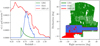 |
Fig. 1 Galaxy number density (left panel) and footprint (right panel) of the LRG sample (green), the ELG sample (blue), and the DES y3 GOLD catalogue (red). The n(z) of DES corresponds to the concatenation of the n(z) on each tomographic bin (Myles et al. 2021). It has been sub-sampled by a factor 20 for clarity. On the right panel, we present the DES footprint with a cut below a declination of −12. |
2 Data
2.1 eBOSS and DES catalogues
The extended Baryon Oscillation Spectroscopic Survey (eBOSS; Dawson et al. 2016) measured thousands of spectra of galaxies and quasars in the range 0.6 < z < 2.4 in order to probe the geometry and growth rate of the Universe over cosmic time. In this work, we study the properties of the emission line galaxies (ELGs) and eBOSS luminous red galaxies (LRGs) combined with the BOSS CMASS sample1. Description of these samples can be found in Ross et al. (2020) and their cosmological analyses in Tamone et al. (2020); de Mattia et al. (2021); Bautista et al. (2021); Gil-Marín et al. (2020). We focused our attention on the South Galactic Cap (SGC), where 121 717 LRGs and 89 967 ELGs were observed in the range 0.6 < z < 1.0 and 0.6 < z < 1.1. In addition to the clustering properties of these galaxies, we aim to extract information from the GGL signal. This is achieved with the shape measurements of DES Year 3 (Y3). We used the main Y3 DES catalogue (referred as ‘Gold’)2 – information on the photometry and shape measurements of this sample can be found in Sevilla-Noarbe et al. (2021); Gatti et al. (2021), while the corresponding cosmological 3 × 2pt analysis is presented in Abbott et al. (2022). The radial distribution and the footprint of each survey are presented in Fig 1. eBOSS and DES overlap in a small portion, around 754 deg2, in the SGC. In the overlapping area, 14 413 244 sources can be used to infer the GGL signal of 44 456 LRGs lenses, while all of the observed ELGs are within the DES footprint3. Although there are more eBOSS galaxies in the North Galactic Cap, there is no overlapping weak lensing survey with precise and robust shape measurements to measure the GGL signal in this pole. Therefore, we only used the clustering measurement in the SGC so that the clustering and lensing signals are correlated.
2.2 The UCHUU simulation
In order to model the observed signals, we relied on the N-body simulation UCHUU (Ishiyama et al. 2021). This simulation was run with GreeM, a massively parallel TreePM code (Ishiyama et al. 2009, 2012), with initial conditions produced by second-order Lagrangian perturbation theory starting at a redshift z = 127. The cosmological flat ΛCDM parameters of the simulation are compatible with the ones measured by Planck Collaboration XIII (2016), (Ωm, Ωb, h, ns, σ8) = (0.3089, 0.0486, 0.6774, 0.9667,0.8159). We note that UCHUU is one of the most precise N-body simulations to date, with 12 8003 dark matter particles with mass 3.27 × 10⁸ h−1 M⊙ in a box of side length L = 2 h−1 Gpc. This large volume enabled us to study a large number of dark matter halos up to a very high mass of M ≈ 1014.8 h−1 M⊙. These halos were identified with the RockStar halo finder (Behroozi et al. 2013). We extracted from the simulation4 the halo and sub-halo catalogues of mass M > 1011 h−1 M⊙ and the particle distribution (sub-sampled by a factor 0.005) at redshifts z = 0.86 and ɀ = 0.7, corresponding to the effective redshift of the ELG and LRG samples, respectively.
3 Halo occupation model
3.1 Standard halo occupation distribution parametrisation
In order to simulate realistic galaxy distributions in the UCHUU simulation, we populated halos using the standard HOD description. For LRGs, we considered the HOD framework first described in Zheng et al. (2005, 2007) and widely used in previous BOSS and eBOSS studies (White et al. 2011; Zhai et al. 2017). For emission line galaxies, we used the Gaussian HOD model (GHOD) (Avila et al. 2020; Rocher et al. 2023a) for central occupation. Hence, we defined the mean central halo occupations as5
![Mathematical equation: $\left\langle {N_{{\rm{cen}}}^{{\rm{LRG}}}(M)} \right\rangle = {{{f_{{\rm{ic}}}}} \over 2}\left[ {1 + {\mathop{\rm erf}\nolimits} \left( {{{\log M - \log {M_{{{\min }^{{\rm{LRG}}}}}}} \over {{\sigma _{{\rm{M}},{\rm{LRG}}}}}}} \right)} \right],$](/articles/aa/full_html/2024/10/aa49574-24/aa49574-24-eq1.png) (1)
(1)
 (2)
(2)
where fic and Ac correspond to completeness factors and the σM correspond to scatters of central occupations. When the samples are complete,  is the halo mass at which half of the halos have a central galaxy.
  always corresponds to the halo mass with maximal probability to host a central galaxy. The satellite occupation is defined as
![Mathematical equation: $\left\langle {{N_{{\rm{sat}}}}(M)} \right\rangle = f(M){\left[ {{{M - \kappa {M_{{{\min }^{{\rm{LRG}}/{\rm{ELG}}}}}}} \over {M_1^{{\rm{LRG}}/{\rm{ELG}}}}}} \right]^\alpha },$](/articles/aa/full_html/2024/10/aa49574-24/aa49574-24-eq5.png) (3)
(3)
 (4)
(4)
where the M16 are the halo masses for which a halo has one satellite galaxy (when the samples are complete), α is the power-law index, and κ is a parameter that allows the cut-off of satellite occupation to vary with halo mass. For the ELG HOD, we assumed the relations given in Table 2 of Avila et al. (2020),
 (5)
(5)
From these mean occupations, the number of central galaxies per halo of mass M then follows a Bernoulli distribution with a mean probability equal to 〈Ncen〉. These galaxies are positioned at the centre of their host halos. The number of satellite galaxies per halo follows a Poisson distribution with mean 〈Nsat〉, with positions sampled from a Navarro-Frank-White (NFW) profile (Navarro et al. 1996). Satellite velocities are normally distributed around the mean halo velocity, with a dispersion being equal to the ones of the dark matter halo particles,
 (6)
(6)
Eventually, the final number density of mock galaxies can be computed as
![Mathematical equation: ${\bar n_{{\rm{gal }}}} = \int {{{{\rm{d}}n(M)} \over {{\rm{d}}M}}} \left[ {\left\langle {{N_{{\rm{cent }}}}(M)} \right\rangle \mid + \left\langle {{N_{{\rm{sat }}}}(M)} \right\rangle } \right]{\rm{d}}M,$](/articles/aa/full_html/2024/10/aa49574-24/aa49574-24-eq9.png) (7)
(7)
and the satellite fraction is given by
 (8)
(8)
Obviously, the mean number density of galaxies is fixed, which gives a constraint on the free parameters of the HOD. For ELG, we followed the methodology described in Rocher et al. (2023a). As the mock clustering is governed by the ratio As/Ac, Ac is a not a free parameter but is instead fixed to provide the desired number density of objects, in our case  by matching
  to Eq. (7). Similarly, for LRG, the HOD is parameterised by (M1,σM,α,κ, fic), and Mmin is fixed in order to obtain twice the mean observed density of the LRG sample (to reduce sample noise), where
  as in Zhai et al. (2017). This is done by matching
  to
to  in Eq. (7). We therefore have three free parameters in our ELG HOD model, θ ⊂ (As, Mmin, α), and five parameters, θ ⊂ (M1,σM,α, κ, fic), with the LRG HOD model. In recent works (Avila et al. 2020; Rocher et al. 2023a,b; Yuan et al. 2022), it is common to enhance this description with extra parameters that describe deviation from the satellite NFW profile and from the velocity assignment of Eq. (6) in order to properly model the anisotropic correlation function. Since we are only interested in describing projected quantities (see Sect. 3.3), we did not introduce these additional parameters. Indeed, the GGL signal, being a real space quantity, is insensitive to galaxy velocities, while redshift space distortion has a subdominant impact on projected clustering (van den Bosch et al. 2013; Rocher et al. 2023a). Eventually, the HOD model described in this section was calibrated against data to provide realistic mocks with clustering properties similar to those of the observations, as explained in Sect. 3.3.
3.2 Extended halo occupation distribution including assembly bias
Since we aim to provide realistic galaxy mocks that are in agreement with observations, we extended our HOD framework with additional parameters to take into account secondary halo properties. This was motivated by studies such as Leauthaud et al. (2017) that found strong differences between the observed galaxy-galaxy lensing signal of CMASS galaxies and the one measured in the mock catalogues using the standard HOD model described above. Here, we followed the formalism described in Xu et al. (2021); Yuan et al. (2022). The standard HOD framework was extended with four additional parameters, two depending on halo properties (specifically the concentration and shape of the halo) and two external properties, namely the local density and local shear (local density anisotropies). Next, we define in practice how we estimated these additional parameters.
First, we defined the halo concentration c and shape e as
 (9)
(9)
with rvir as the virial radius, rs as the scale radius of the density profile, and b/a as the ratio between the major and semi-major axes of the dark matter halo ellipsoid. These halo properties were directly extracted from the halo catalogues. The concentration was measured by fitting an NFW profile to each halo, while shapes were determined with the method of Allgood et al. (2006).
To specify the halo environment within the simulation, we employed two different techniques. The first one consisted of finding for each halo all neighbouring halos (including subhalos) beyond its virial radius but within rmax = 5 h−1 Mpc of the halo centre. This was done with the Python pack- agescipy-Kdtree7, which keeps track of pairs of halo per object. The rmax scale was chosen in Yuan et al. 2021, as values of rmax in the range ≈4–6 h−1 Mpc were found to better reproduce the clustering of CMASS galaxies. In particular, it was shown by the authors that the goodness of fit depends on the scale at which the environment is defined (see Fig. 8 of Yuan et al. 2021). After summing up the mass of all these neighbouring halos, the environmental parameter fenv could then be computed as
 (10)
(10)
where  corresponds to the mean environment mass within a given halo mass bin dM. This environmental parameter hence corresponds to the halo over-density in an annulus around each halo. We computed
  in the logarithm mass range [11,15.0] h−1 Mpc in bins of dex dM = 0.1 h−1 Mpc.
The second method consisted of painting the dark matter particle field onto a mesh in order to evaluate the over-density field δ(x) (Paranjape et al. 2018; Delgado et al. 2022; Hadzhiyska et al. 2023b). The field δ was then smoothed with a Gaussian kernel of radius R and interpolated at the position of each halo. This was done with the Python package nbodykit8. From the smoothed density field, we further defined the environmental shear, which quantifies the amount of local density anisotropy. First, we computed the tidal tensor field as
 (11)
(11)
where the normalised gravitational potential ψR (x) obeys the Poisson equation
 (12)
(12)
This was easily done in Fourier space, the expression for the tidal tensor being equal to
 (13)
(13)
from which we determined the tidal shear  :
:
 (14)
(14)
where the λ correspond to the eigenvalues of Tij. Different definitions of the smoothing radius have been used in the literature. Delgado et al. (2022) used a top hat filter of fixed size: 5 h−1 Mpc9. Hadzhiyska et al. (2023b) estimated the density field with a Gaussian filter at different smoothing scales and selected for each halo the closest smoothing scale to the virial radius of the halo, rounding up. In Paranjape et al. (2018), they found that the correlation between large-scale linear bias and local shear was maximum at scales of four to six times the virial radii. We therefore adopted two definitions for our smoothing scale. The first one is a constant smoothing of size  Mpc, from which we determined
  for each halo. Our second definition uses a smoothing scale of 2.25 rvir for each halo, from which we determined the local density and local shear. The density field was smoothed from 1 to 5 h−1 Mpc with a step dx = 0.25 h−1 Mpc and interpolated at the position of each halo to determine δR(x) for R = 2.25 rvir.
These secondary halo properties were used to modify the two mass parameters of the HOD model, Mmin and M1, as
 (15)
(15)
 (16)
(16)
where fA and fB correspond to the distributions of internal (either concentration or shape) and environmental (either shear or density) properties of the halos. This type of effective description that modifies central and satellite occupation based on secondary properties was also proposed in Hadzhiyska et al. (2023a). The authors found that the simulation-predicted quantities Ncent(M, fA, fB) and Nsat(M, fA, fB) for each mass bin are well approximated by hyper-plane surfaces, which are nearly constant over mass. These distributions were normalised in the range [−1,1] within the mass bins defined to compute the environmental factor fenv in Eq. (10). This was done by first taking the natural logarithm of each quantity (1+δ for the density) before scaling and normalising it around zero. Taking the logarithm of each quantity first has the advantage of keeping the shape of their distributions intact, as we are much less sensitive to outliers that squeeze the distribution after normalisation. We present these distributions in Appendix B. The high volume of UCHUU enabled us to probe the assembly bias and environmental dependencies on halo occupation up to very high halo masses, M = 14.8 h−1 Mpc, with more than 100 halos in the mass bin [14.7,14.8] h−1 Mpc. Extra parameters in Eq. (15) were fixed to zero above this threshold, as higher masses bins are not populated enough for a robust statistical description.
Our extended HOD framework therefore has seven parameters for an ELG HOD θ ⊂ (As, Mmin, α, Acent, Bcent, Asat, Bsat) and nine parameters θ ⊂ (M1,σм,α,κ, fic, Acent, Bcent, Asat, Bsat) for an LRG HOD. In the following, we test different combinations in Eqs. (15)–(16), between internal halo properties fA (concentration and shape) and the local environment fB (density and shear).
3.3 Fitting procedure
Our fitting method uses the HOD model described above to populate dark matter halos with galaxies for which clustering and lensing statistics are measured and compared to the ones of the data. Here, we are interested in the projected correlation function, which is almost insensitive to the effect of redshift space distortions at small scales. We computed the galaxy anisotropic two-point function ξ (rp, π) as a function of galaxy pair separation along (π) and transverse to the line of sight (l.o.s.;rp). Integrating over the l.o.s. yielded
 (17)
(17)
We used the Dark Energy Spectroscopic Instrument (DESI, DESI Collaboration 2016) wrapper, pycorr10, around the corrfunc package (Sinha & Garrison 2020) to compute ξ (rP, π) with the natural estimator, which normalises galaxy pair counts to analytical estimation of random pairs in a periodic box. For the data, we used the minimum variance Landy & Szalay (1993) estimator
 (18)
(18)
with R as a random catalogue with the same angular and redshift distribution as the data. We applied to each galaxy and random catalogue the total weight w = wnoz wcp wsystwFKP (see Ross et al. (2020) for an in-depth definition of each individual weight). Briefly, wnoz corrects for redshift failures, wsyst corrects for spurious fluctuation of target density due to observational systematic effects, FKP weights (Feldman et al. 1994) are optimal weights used to reduce variance in clustering measurements, and close-pair weights wcp correct for fibre collisions. Correcting for fibre collision is an important matter in our case, as we want to extract information from the one-halo regime in order to constrain the satellite distribution in our HOD model. Traditionally, these weights are applied by up-weighting observed galaxies in a collision group.
While this method provides a good correction scheme at large scales, which is enough for the study of galaxy anisotropic clustering, it fails on smaller scales, and we therefore needed another method to correct for fibre collisions. In particular, we used the pairwise-inverse probability (PIP) and angular upweighting (ANG) weights described in Mohammad et al. (2020). These weights were shown to properly account for fibre collisions at small separations. However, PIP weights were only produced for eBOSS galaxies, and we therefore only applied ANG weights to the combined sample (including the cp weights), as they provide sufficient correction below 1 h−1 Mpc. For wp(rp), we used 13 logarithmic bins in rp between 0.2 and 50 h−1 Mpc, with πmax = 80 h−1 Mpc. In addition to the clustering, we also fit the GGL signal, similar to the work of Contreras et al. (2023b), observed with eBOSS lenses around DES sources in order to further constrain the assembly bias parameters. The measured GGL differential excess surface density is defined as
 (19)
(19)
where the mean projected surface density is defined as
 (20)
(20)
The projected surface density Σgm(r) can be written as a function of the galaxy-matter cross-correlation as (Guzik & Seljak 2001; de la Torre et al. 2017; Jullo et al. 2019)
 (21)
(21)
with the mean matter density  constant in redshift in co-moving coordinates. The galaxymatter correlation ξgm function was measured in the range [5 × 10−3,150] h−1 Mpc with 41 logarithm bins by cross-correlating galaxy mock catalogues with the dark matter particles of the simulation, sub-sampled by a factor of 2000. With this sub-sampling factor, we could accurately predict ΔΣ (we omit the gm subscript in the following parts of the paper) as in Contreras et al. (2023a), whose authors claimed that sub-sampling the matter field by a factor ~0.0003 ensures robust measurement of ΔΣ with sub-percent precision across all the ranges considered in their analysis. We checked this statement with the simulation used in this work. The measurements of ΔΣ performed with particles sub-sampled by a factor 0.00511 or 0.0005 are the same. We then estimated Σ(r) by integrating Eq. (21) up to 100 h−1 Mpc. The estimation of ΔΣ was then compared to the one observed in the data, which is computed as (Jullo et al. 2019)
 (22)
(22)
where ɀs and ɀ1 correspond to the source and lens redshift, respectively, and є+ represents the tangential component of a source ellipticity around a lense. The subtraction around random lenses reduces the contribution of lensing systematics and leads to a reduced variance on small scales (Singh et al. 2017). The critical density Σcr is defined as
 (23)
(23)
where DS, DLS, DL are the observer-source, lens-source, and observer-lens angular diameter distances. We measured ΔΣ(rp) with 13 (11 for the ELG) logarithmic bins in the range between 0.2 and 20 h−1 Mpc with the python package dsigma12 (Lange & Huang 2022). We used Metacalibration shape measurements and corrected for potential systematic effects induced by this method. We used for photometric redshifts of source galaxies the ones estimated with the Directional Neighbourhood Fitting (DNF) algorithm (De Vicente et al. 2016). Errors in photo- ɀ measurements can lead to bias in the estimation of ∆Σ. We matched DES galaxies with galaxies observed spectroscopically with BOSS and eBOSS. While these samples are not representative of DES galaxies, they can however be used to obtain a rough estimate of the bias introduced by the photo-ɀ. We found that photo-ɀ leads to an underestimation of the observed signal by approximately 3–5% at all scales. Since this effect is subdominant compared to the S/N of our measurements, we did not include it. We also did not include any Boost factor correction (Miyatake et al. 2015), as we have found that it has nearly no impact on our measurements, even at the smallest scale.
When computing the correlation functions for the data in Eqs. (18) and (22), we assumed the UCHUU cosmology to compute radial distances from redshift. We then compared the HOD clustering and lensing signals to the observed ones in eBOSS by means of a likelihood analysis:
 (24)
(24)
where θ is the set of HOD parameters, ∆ is the data-model difference vector, Np is the total number of data points, and Ψij is the precision matrix, the inverse of the covariance matrix. The covariance matrix is determined given the observational measurements by jackknife (JK) sub-sampling with N = 100 patches. Since all ELGs are within the DES footprint, we could use the same JK regions for the clustering and lensing measurements in order to estimate the cross-correlation between wp and ΔΣ. For the LRG, only about a third of the sample is within DES footprint. We decided to use the whole sample to estimate wp in order to get a sufficient S/N measurement. Since ∆Σ is only measured within the overlapping footprint, the crosscovariance cannot be estimated through the jackknife method, and we assumed it to be zero. We checked with the ELG sample that this assumption does not change the results significantly: the jackknife cross-covariance is mainly dominated by noise.
Our fitting procedure corresponds to the one described in (Rocher et al. 2023a,b). The parameter space is first sampled with a quasi-uniform grid, which serves as a training sample for a Gaussian process regressor and technical details. Here, we used the Gaussian process implemented in sklearn13. For each sampled point in the parameter space, the clustering and lensing signals are averaged over ten realisations to reduce stochastic noise from halo occupation. We then repeated, iteratively, the following procedure: We used a Markov chain Monte Carlo (MCMC) sampler, here emcee14 (Foreman-Mackey & al. 2013), to sample our parameter space given our surrogate model generated by the Gaussian process regressor. Specifically, we ran 50 chains of 5000 points in parallel, with the first 500 points being discarded in each chain. We then randomly picked three points within our final MCMC chains from which we computed the likelihood. We then added these points to the initial training sample and re-trained our Gaussian process. In Rocher et al. (2023a), they found that iterating up to N = 800 from a training sample of Nini ≈ 1000 was enough to get robust contours. These findings are highly dependent on the parameter space one wants to explore and the dynamic range of the likelihood. While we do find the same conclusion for an ELG HOD, the degree of degeneracy of an LRG HOD calls for a higher number of iterations. We therefore used Nini = 1000 (resp. 2000) and N = 1000 (resp. 2000) for the ELG (resp. LRG) fit. We checked that our results are robust to these choices. Additionally, we refer the reader to (Rocher et al. 2023a) for more details on the performance of the Gaussian process emulator. Briefly, the authors compared their results with the ABACUS HOD pipeline (Yuan et al. 2021) and found strong agreements between the two methods. The main difference between the implementation of Rocher et al. (2023a) and ours is that the authors only picked one point in each chain for each iteration, while we decided to pick three per iteration. The reason for this decision is computation speed. We found that for a high number of points, the Gaussian process regression takes a longer time to compute than three averaged HOD realisations. The key element is to have a high enough number of points in the region where the likelihood is minimal to have robust contour estimation with the Gaussian process.
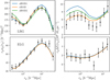 |
Fig. 2 Best-fit HOD models for LRG (top) and ELG (bottom). The subscript ‘s/e’ denotes the standard and extended HOD model. The extended model here corresponds to our fiducial configuration, where the concentration and an annular definition of δ are used as additional parameters. The points with error bars correspond to the measured wp (left) and the ∆Σ (right) signals. The blue lines (sHOD1) correspond to a fit to the projected correlation function wp only, while the green (SHOD2) and orange lines (eHOD) correspond to standard and extended HOD fits including the measurement of ∆Σ in the fitting pipeline. The extended HOD model provides a good description of both the clustering and lensing signal. We did not perform any standard HOD fit to the combined wp + ∆Σ vector for ELGs (sHOD2), as the standard HOD fit to wp only already agrees well with the ∆Σ measurement. |
Best-fit parameters of the LRG HOD for all configurations defined in the main text.
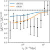 |
Fig. 3 Difference between the observed galaxy-galaxy lensing signal (points with error bars) of eBOSS LRGs with the prediction of a standard HOD (sHOD) determined by fitting the projected correlation function wp only. The continuous line in blue represents an sHOD fit to wp + ΔΣ, while the orange line corresponds to the extended HOD model. |
4 Halo occupation distribution fit
4.1 Luminous red galaxies
As a baseline configuration for the extended HOD (eHOD) model, we used the concentration as a proxy of assembly bias and the local density, described as an annular definition of the density field δ, following the formalism of Yuan et al. (2022). We emphasize that the annular definition of local density might be prone to sub-halo identification and thus simulation resolution. However, given the properties of the UCHUU simulation (see Sect. 2.2), we did not consider this potential source of bias in our analysis. We present in Fig. 2 the best-fit results obtained with the standard (s) and extended (e) HOD models. The standard model sHOD2 and the extended model both fit the combined wp, ΔΣ data vector, while the sHOD1 model only fits wp. Best-fit values are given in Table 1, while full posterior distributions and prior information can be found in Appendix C. For the sHOD1, one can see that the model over-predicts the signal at scales around 10 h−1 Mpc while obtaining a satellite fraction of 8%, slightly lower than what was obtained in Alam et al. (2020); Yuan et al. (2022) and 50% below the best-fit value of Zhai et al. (2017). We found that this difference was due to noise in the jackknife covariance estimate of wp. When we performed a fit only considering the diagonal elements, we obtained a satellite fraction of 11%, the model matches well the peak at 10 h−1 Mpc but in turn provides a poor fit at scales 1–3 h−1 Mpc, similar to the observed fit for the sHOD2 case and an issue in the modelling also reported in Zhai et al. (2017). The introduction of secondary HOD parameters enabled us to provide a better description of the small and intermediate scales of wp while also yielding a more accurate description of ∆Σ, decreasing the reduced chi-square from  down to
  , an improvement mainly due to a better description of ∆Σ on the scales below 3 h−1 Mpc.
Figure 3 displays the ratio of ∆Σ measurements in the data and as measured in the mocks generated by sHOD2 and eHOD models (calibrated on both wp and ∆Σ measurements), compared to the ∆Σ measurement as measured in the mock generated by the sHOD1 (calibrated only against the projected clustering wp). The standard model (dashed line) over-predicts the GGL signal by 30–40% at scales below 10 h−1 Mpc, while a combined fit (blue solid line) poorly alleviates this issue, with a slight improvement of only ≈5–15%. With the eHOD model, we observed an improvement of 20% on scales between 2–10 h−1 Mpc and a really good match to the data at lower scales. This better goodness of fit is mainly achieved by incorporating a dependence on the local density environment (Yuan et al. 2021; Hadzhiyska et al. 2023a). Thus, adding secondary halo parameters to the HOD models helps reproduce the lensing signal at small scales and gives a partial answer to the lensing-is-low problem. Indeed, baryonic feedback, not considered in this work, smooths out the matter distribution, also contributing to a decrease of ∆Σ (Amodeo et al. 2021).
We present in Fig. 4 the posterior distributions of each HOD fit. The better description of ∆Σ with the sHOD2 was achieved by lowering the mass threshold M1 and Mmin (see also Table 1), above which central and satellite galaxies occupy dark matter halos. We observed the same trend for the eHOD, interestingly with a higher best-fit value for Mmin compared to the sHOD2 case. To maintain a similar galaxy bias between the eHOD and sHOD1 models, galaxies in lower mass halos should therefore be located in higher density peaks. This is what we obtained in the posterior distributions of Fig. 5. A negative value of Bcent implies that halos located in denser environments are more likely to be populated, as a decrease of  in Eq. (15) increases the probability of populating such halos, a result also found for CMASS galaxies (Yuan et al. 2022) and in hydrodynamical simulations (Artale et al. 2018).
In recent studies, halo occupation was found to be strongly dependent on formation time (Zehavi et al. 2018; Artale et al. 2018) and concentration (Bose et al. 2019; Delgado et al. 2022), as both variables are correlated (Wechsler et al. 2002), although in a non-trivial way (Gao & White 2007). The conclusion from these analyses was that at low mass, central galaxies are more likely to be hosted by more concentrated, early-formed halos. This trend reverses at higher mass due to the contributions of satellite galaxies. However, given our measurements, the only parameter that is well constrained is Bcent, being non-zero at the 3σ level, while all the other parameters are consistent with zero at the 1σ level. Hence, based on our analysis, we cannot draw a proper conclusion on the impact of assembly bias on halo occupation. Similar to Yuan et al. (2022), we also find that including secondary assembly bias parameters (or just fitting ΔΣ) does increase the satellite fraction. This can be explained by the fact that central-particle correlation is dominant on small scales (Leauthaud et al. 2017). Thus, increasing the satellite fraction will lower the central contribution and the low scales ΔΣ signal. For completeness, we present the full posterior distribution of the extended HOD in Appendix C. In Sect. 3.1, we made two approximations that might impact the result present in this section, mainly the choice of number density and an assumption of a simple NFW profile. We show in Appendix A that our statistically significant result, the environmental dependence on halo occupation, is robust with respect to our fiducial choices. However, we did not consider other physical effects that impact our GGL signal.
As demonstrated in Chaves-Montero et al. (2023), satellite segregation and baryonic feedback are the two main sources, after assembly bias, that create the lensing-is-low problem. Clearly, including these effects would modify the interpretation of our results. Study of these effects is out of the scope of this paper, as our main goal is to investigate how small-scale variations of ΔΣ can impact cosmological analysis of anisotropic clustering plus lensing signal (see Sect. 5).
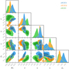 |
Fig. 4 Posterior contours of the sHOD1 (in blue), sHOD2 (in orange), and eHOD (in green) in our baseline configuration (including concentration and annular density as additional parameters) for the LRG sample. One can observe that the extra parameters contained in the eHOD model have a strong impact on the posterior distributions. |
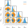 |
Fig. 5 Posterior contours of the assembly bias and environmental parameters in our baseline configuration (see Sect. 4.1). For the LRG, the negative value of Bcent, detected at 3σ, indicates that LRG centrals most likely occupy a dense environment. A negative value of Asat at the 1σ level indicates that satellite galaxies could be preferentially located in more concentrated halos than average. For the ELGs, all parameters are consistent with zero at the 1σ level, suggesting that ELGs do not exhibit significant assembly bias or environmental dependencies. |
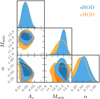 |
Fig. 6 Posterior contours for the sHOD (in blue) and eHOD (in orange) models for the ELG sample. Taking into account assembly bias parameters has little impact on halo occupation. |
Posterior and best-fit results for the ELG HOD.
4.2 Emission line galaxies
The best-fit results for ELGs are represented in the bottom panel of Fig. 2, while the posterior contours are shown in Fig. 6 with the corresponding constraints in Table 2. We did not observe significant differences between the standard and the extended HOD framework when considering either the best-fit model or the full posterior distribution. Both models provide a similar goodness of fit and reproduce the observations, with a χ2 = 23.1 and 22.0 respectively for the sHOD and eHOD models, resulting in a worse reduced χ2 for the eHOD, as the four additional free parameters do not significantly improve the fit. From the posterior distributions in Fig. 5, one can see that all the secondary parameters are consistent with zero at the 1σ level. In the literature, it was shown that ELGs are preferentially located in denser regions than average (Artale et al. 2018; Delgado et al. 2022) and in more concentrated halos (Zehavi et al. 2018; Artale et al. 2018; Rocher et al. 2023b). This is in agreement with our negative best-fit values for Acent and Bcent , even though we cannot derive more decisive conclusions from our analysis.
In addition, we found a satellite fraction of 10.4% for the sHOD, significantly lower than that reported in Avila et al. (2020), fsat = 22%. However, for ELGs, the mean satellite occupation is independent of that of the centrals, which means that an ELG satellite can orbit around a non-ELG central. Thus, it only contributes to the two-halo term of the ELG auto-correlation function, affecting the amplitude of the linear bias of the galaxy sample. The lower satellite fraction (compared to Avila et al. 2020) can be explained by the fact that our mean value for Mmin = 12.19 is larger than that reported in Avila et al. (2020), Mmin = 11.71 and that we allowed α to vary, resulting in a different satellite occupation over halo mass. In Rocher et al. (2023b), when they include strict conformity, that is, satellite galaxies can only populate the halo in the presence of a central ELG, they report a very small fraction of satellite of ≈2–3%. For DESI ELG, strict conformity is needed in order to provide a positive value for α, which is predicted by semi-analytical models (Gonzalez-Perez et al. 2018, 2020).
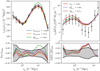 |
Fig. 7 Result for different combinations of assembly bias (concentration and shape) and local environments (density and shear) parameters. Top panels present the measurements, while the bottom panels show the relative differences. Nearly all the models provide similar best-fitting clustering predictions, lensing predictions, and goodness of fit results except the shear measured with a Gaussian Kernel of size 2.25 h−1 Mpc, which has a slightly worse goodness of fit. |
4.3 Dependence on parameter choices
We present in Fig. 7 multiple eHOD best-fit models for different configurations. We tested as a proxy for the environment either the local shear or the local density, combined with internal properties, that is, concentration or shape of the dark matter halos. As a reminder, the baseline configuration corresponds to the case where we apply to Eq. (15) fA = concentration and fB = δannulus, with δannulus calculated by summing the mass of neighbouring halos. Estimating the local density field with this definition provides a better description of the observed LRG signal, with a  improved by
  , compared to the case where the density field is estimated on a mesh with a Gaussian smoothing kernel of size = 2.25rvir, with
  . These results are in agreement with those of Yuan et al. (2022), who found that estimating the density field with a Gaussian kernel of a fixed size of 3 h−1 Mpc yields no significant improvement compared to the sHOD. Instead of the concentration of the dark matter halo, using its shape as a proxy for assembly bias provides nearly indistinguishable best-fit model results. The resulting constraints, presented in Table 1 and in Appendix C, suggest that red galaxies preferentially occupy more ellipsoidal halos than average, as the best-fitting value Acent is positive when either considering shear or density as external property. The two extra configurations including the local density are in agreement with the baseline configuration, which is in favour of a negative value for Bcent such that galaxies preferentially occupy denser environments.
Using the local shear instead of the local density also provides good  values when the tidal tensor is computed with a Gaussian kernel of size 2.25 rvir. The best
  value is obtained when combining the local shear with the halo shape,
  . It reproduces the small scales of ΔΣ better but gives a slightly worse fit around the peak of wp observed at 10 h−1 Mpc. Surprisingly, using the local shear with a fixed Gaussian smoothing of size 2.25 h−1 Mpc provides the worst
  value out of all configurations. This demonstrates that local density anisotropy should be considered at halo scales to retrieve the maximum amount of information, as explained in Paranjape et al. (2018). Our results suggest that galaxies preferentially occupy more anisotropic environments, in agreement with Delgado et al. (2022), who found this correlation for low-mass halos, and with DESI ELGs (Rocher et al. 2023b).
5 Cosmological fit
In the current analysis, perturbative and semi-analytical models that are aimed at extracting cosmological information from the observations were tested intensively against galaxy mock catalogues. In eBOSS analysis (Rossi et al. 2021; Alam et al. 2021), different HOD models were used in order to quantify the modelling systematics of redshift-space distortion models. The authors found consistent results amongst a large variety of HOD models that validated the accuracy of the theoretical models.
5.1 Theoretical models
In the analyses of de la Torre et al. (2017); Jullo et al. (2019), the measured anisotropic clustering ξ(r⊥, r∥) at an effective redshift ɀ was combined at the likelihood level with lensing measurements of ΔΣ in order to provide direct constraints on the growth rate of the structure f (ɀ), the amplitude of matter fluctuation σ8(ɀ), and the present time matter density Ωm. These studies extracted information at scales below 3 h−1 Mpc, where our HOD models, as illustrated in Fig. 2, show significant differences that might introduce biases when quantifying modelling systematics of ΔΣ.
In this study, We performed the cosmological analysis of galaxy catalogues populated with the standard and extended HOD framework in order to test the accuracy of a combined analysis of galaxy clustering and galaxy-galaxy lensing. We considered as a redshift space model the TNS (Taruya et al. 2010) model extended to non-linearly biased tracers, hereafter referred to as TNS, described and robustly tested in detail in Bautista et al. (2021). The expression for the redshift space power spectrum of biased tracers is given by
![Mathematical equation: $\eqalign{ & {P^s}(k,v) = D\left( {kv{\sigma _v}} \right)\left[ {{P_{{\rm{gg}}}}(k) + 2{v^2}f{P_{g\theta }}(k) + {v^4}{f^2}{P_{\theta \theta }}(k)} \right. \cr & & & \left. { + {C_A}\left( {k,v,f,{b_1}} \right) + {C_B}\left( {k,v,f,{b_1}} \right)} \right], \cr} $](/articles/aa/full_html/2024/10/aa49574-24/aa49574-24-eq65.png) (25)
(25)
where k is the wave-vector norm, ν is the cosine angle between the wave-vector and the l.o.s., θ is the divergence of the velocity field v defined as θ = −∇·v/(aHf), and f is the linear growth rate parameter. The terms CA (k, ν, f ) and CB(k, ν, f ) are the two correction terms given in Taruya et al. (2010), which reduce to one-dimensional integrals of the linear matter power spectrum. The damping function D(kνσv) describes the Fingers-of-God effect induced by random motions in viri- alised systems, inducing a damping effect on the power spectra. We adopted a Lorentzian form,  , where σv represents an effective pairwise velocity dispersion treated as an extra nuisance parameter. The expressions of the real space quantities Pgg , Pgθ, and Pgm are given following the bias expansion formalism of Assassi et al. (2014):
 (26)
(26)
where each function of k is a one-loop integral of the linear matter power spectrum Plin, whose expression can be found in Simonović et al. (2018). The expressions of  , and
, and  are the same as
  except that the G2 kernel replaces the F2 kernel in the integrals. To estimate the velocity divergence power spectra Pθθ and Pδθ, we used the Bel et al. (2019) fitting function, which depends solely on σ8:
 (27)
(27)
with the expressions of each parameter given in Bel et al. (2019); Bautista et al. (2021). The linear matter power spectrum was estimated with camb (Lewis & Challinor 2011)15, while the nonlinear power spectrum Pδδ was estimated with the latest version of HMcode (Mead et al. 2021). This is different from Bautista et al. (2021); Paviot et al. (2022), where we used the response function formalism respresso described in Nishimichi et al. (2017). Indeed, the latest version of HMcode provides nearly indistinguishable (at least in configuration space) baryon acoustic oscillation damping due to non-linear effects while also matching the power spectrum of respresso at a higher k.
The TNS correlation function multipole moments were finally determined by performing the Hankel transform on the model power spectrum multipole moments,
 (28)
(28)
where jℓ and Lℓ denote the spherical Bessel function and Legendre polynomials of order ℓ. The Hankel transform, that is, the outer integral in the above equation, was performed rapidly using the FFTlog algorithm (Hamilton 2000). Under the limber approximation Limber (1953), the expression of the galaxygalaxy lensing signal is given by Marian et al. (2015)
 (29)
(29)
with J2 as the second-order Bessel function of first kind and ρm as the co-moving matter density, constant over cosmic time. In order to remove the contribution of non-linear modes, we computed the annular differential excess surface density (ASAD) estimator given by (Baldauf et al. 2010)
 (30)
(30)
where R0 corresponds to a cut-off radius, below which the signal is damped.
In addition, we parametrised the Alcock-Paczyński (AP) distortions (Alcock & Paczynski 1979) induced by the assumed fiducial cosmology in the measurements via two dilation parameters that scale transverse, α⊥, and radial, α∥, separations. These quantities are related to the co-moving angular diameter distance, DM = (1 + ɀ)DA (ɀ), and Hubble distance, DH = c/H(ɀ), respectively, as
 (31)
(31)
 (32)
(32)
where c is the speed of light in the vacuum and ɀeff is the effective redshift of the sample. We applied these dilation parameters to the theoretical TNS power spectrum Ps(k, ν) in Eq. (28) so that Ps(k, ν) → Ps(k′ , ν′), where
![Mathematical equation: ${k^\prime } = {k \over {{\alpha _ \bot }}}{\left[ {1 + {v^2}\left( {{1 \over {F_{{\rm{AP}}}^2}} - 1} \right)} \right]^{1/2}},$](/articles/aa/full_html/2024/10/aa49574-24/aa49574-24-eq77.png) (33)
(33)
![Mathematical equation: ${v^\prime } = {v \over {{F_{{\rm{AP}}}}}}{\left[ {1 + {v^2}\left( {{1 \over {F_{{\rm{AP}}}^2}} - 1} \right)} \right]^{ - 1/2}},$](/articles/aa/full_html/2024/10/aa49574-24/aa49574-24-eq78.png) (34)
(34)
and FAP = α∥/α⊥. The terms ΔΣ and Υ, being projected quantities, are only distorted by the perpendicular distortion factor
 (35)
(35)
Given a theoretical model for ξℓ and ΔΣ (Υ), we could perform a cosmological analysis assuming a Gaussian likelihood as defined in Eq. (24). Here, our data vector is the concatenation of the redshift-space multipoles with the galaxygalaxy lensing signal, with the free parameters of the model  , with
  being fixed to the Lagrangian prescription as
  (Saito et al. 2014). It is worth noting that as the TNS corrections and the galaxy bias expansion are functions of the linear power spectrum only, these can be rescaled at each iteration by the normalisation σ8. The non-linear power spectrum evaluated with HMcode was first sampled into a broad range of σ8 and then interpolated at any value of σ8 within our prior. Specifically, we computed Pδδ in the σ8 range [0.1,1.2] with a step size of dσ8 = 0.025. Hence, the only quantities that we re-computed at each iteration were the real space quantities Pθθ and Pδθ. We assumed as a fiducial cosmology, the cosmology of the UCHUU simulation such that AP distortions should be equal to unity.
5.2 Covariance matrices
The covariance matrices were estimated with analytical prescriptions. The Gaussian covariance for the multipoles of the correlation function is given by (Grieb et al. 2016)
 (36)
(36)
where the  correspond to bin-averaged spherical bessel functions,
 (37)
(37)
with Vsi as the volume element of the shell. The expression for  is given by
![Mathematical equation: $\eqalign{ & \sigma _{{\ell _1}{\ell _2}}^2(k) \equiv {{\left( {2{\ell _1} + 1} \right)\left( {2{\ell _2} + 1} \right)} \over {{V_{\rm{s}}}}} \cr & \,\,\,\,\,\, \times \int_{ - 1}^1 {{{\left[ {P(k,\mu ) + {1 \over {\bar n}}} \right]}^2}} {{\cal L}_{{\ell _1}}}(\mu ){{\cal L}_{{\ell _2}}}(\mu ){\rm{d}}\mu , \cr} $](/articles/aa/full_html/2024/10/aa49574-24/aa49574-24-eq87.png) (38)
(38)
with Vs as the volume of the periodic box. The expression for the Gaussian covariance of ΔΣ is given by Marian et al. (2015)
![Mathematical equation: $\eqalign{ & {\mathop{\rm Cov}\nolimits} [\widehat {\Delta \Sigma }]\left( {{R_i},{R_j}} \right) = {1 \over {{A_s}}}{\left( {{\rho _{\rm{m}}}} \right)^2}\int {{{{{\rm{d}}^2}{k_ \bot }} \over {{{(2\pi )}^2}}}} {{\bar J}_2}\left( {{k_ \bot }{R_i}} \right){{\bar J}_2}\left( {{k_ \bot }{R_j}} \right) \cr & \,\,\,\,\,\,\,\,\,\,\,\,\,\,\,\,\,\,\,\,\,\,\,\,\,\,\,\,\,\,\,\,\, \times \left\{ {\left[ {{P_{\delta \delta }}\left( {{k_ \bot }} \right) + {1 \over {{{\bar n}_p}}}} \right]\left[ {{P_{{\rm{gg}}}}\left( {{k_ \bot }} \right) + {1 \over {{{\bar n}_g}}}} \right] + P_{{\rm{gm}}}^2\left( {{k_ \bot }} \right)} \right\}, \cr} $](/articles/aa/full_html/2024/10/aa49574-24/aa49574-24-eq88.png) (39)
(39)
where As is the surface area of the box. The  corresponds to bin-averaged Bessel functions, computed in the same way as in Eq. (37) by integrating over the surface element instead. In Eqs. (36)–(39), we assumed linear theory for the power spectra such that
  , and
, and  (Kaiser 1987), with β = f /b. We inferred the value of f from the UCHUU cosmology at the effective redshift of the LRG and ELG sample, respectively ɀ = 0.7 and ɀ = 0.86, while the values of b1 were taken from Bautista et al. (2021); Tamone et al. (2020). The shot-noise terms
  and
and  correspond to the number density of dark matter particles and galaxies in the simulation box. No analytical cross-covariance exists between ΔΣ and the ξℓ, so we approximated it to be zero. To estimate the covariance of Υ, we generated a sample of a thousand ΔΣ from a multivariate normal distribution, given the ΔΣ covariance estimate. We then applied Eq. (30) to each fake sample by considering its mean value for ΔΣ(R0). This had the effect of reducing the noise in the final covariance estimation.
5.3 Analysis choices
We measured the multipoles of the correlation function, the monopole, quadrupole, and hexadecapole with bins of size 5 h−1 Mpc in the range between 0 and 150 h−1 Mpc. We measured ΔΣ with 22 and 16 logarithm bins in the range between 10−1 and 102 h−1 Mpc for LRGs and ELGs, respectively. This binning was chosen for each sample given the S/N of the observations. Since our redshift-space model follows the exact same implementation as in Bautista et al. (2021), we performed a fit of the multipoles on the scales determined in their analysis, which provides unbiased cosmological constraints for an LRG-like sample. These scale cuts were determined by testing the TNS model against the BOSS N-body NSERIES mocks, which were produced to match the clustering amplitude of CMASS galaxies. Since the BOSS CMASS and eBOSS LRG samples have a similar bias, the scale cuts determined with the NSERIES mocks were used to determine the cosmological constraints on the DR16 eBOSS LRG sample (Bautista et al. 2021). We therefore used the minimum fitting range determined in their analysis, and we fit the multipoles (monopole, quadrupole, and hexadecapole) between 25 and 140 h−1 Mpc for the LRG sample. In theory, one could fit ELGs clustering down to smaller scales, as these galaxies are (i) at a higher redshift and (ii) located in lower dense regions. However, we kept the same range in our fitting procedure between the two samples, with the scale cut for an ELG-like sample being conservative. We tested the accuracy of the TNS model as a function of different minimum scales used when fitting either ΔΣ or Υ. The maximum scale that we used is 80 h−1 Mpc, as Limber approximation breaks down on larger scales. The fits were performed on the average of ten HOD realisations to be robust to stochastic variation due to halo occupation.
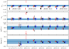 |
Fig. 8 Results from the cosmological fit. Circle points with error bars correspond to the fit of the LRG sample at redshift ɀ = 0.70 populated with the standard and extended HOD framework, while the triangles correspond to the fit of ELGs at redshift ɀ = 0.86. The value of f and σ8 for LRGs (ELGs) are 0.814 (0.849) and 0.570 (0.529) at the redshift ɀ = 0.70(0.86). Values in parentheses correspond to the minimum scale used in the fit in megaparsec per h. The shaded area corresponds to a 10% variation around the fiducial value of each parameter. |
5.4 Results
We present in Fig. 8 the results of the MCMC chains of the combined ξl + ΔΣ fit. Here, the inference pipeline was done with the nautilus sampler16 (Lange 2023). Each chain was stopped after reaching an effective number of 200 000 points, and sampled points in the exploration phase were discarded. We present in Table 3 the corresponding constraints. As expected, we obtained unbiased constraints when fitting only the clustering while fixing the value of σ8 (ɀ) to the fiducial value of the simulation.
However, in the scenario where σ8 was allowed to vary, we observed a strong degeneracy between f and σ8 that is not captured properly by the model given the amount of information present in the multipoles. It is only when combining anisotropic clustering with galaxy-galaxy lensing measurements that one can break this degeneracy. For the LRG mocks, our model provides unbiased constraints on each cosmological parameter, regardless of the HOD, on scales above 3 h−1 Mpc for ΔΣ, with the constraints on the eHOD that seem to converge faster towards consistent results. This is surprising given the observed difference in Fig. 2. The main difference comes from the goodness of fit, with the TNS model providing a better description of the ΔΣ measured with the eHOD galaxy population, Δχ2 ≈ 20 compared to the sHOD. The fact that the TNS model provides a good fit,  , for the eHOD measurements suggests that our model is also capable of yielding a good description of the observations down to a scale of ≈3 h−1 Mpc, in agreement with the result of de la Torre et al. (2017).
It is important to note that these results provide a quantitative description of how small-scale variations of ΔΣ impact cosmological analysis. Indeed, we did not consider satellite segregation and baryonic feedback in this work. Including these effects would most likely impact the evolution of cosmological constraints as a function of scale but would not change the observed trends, for example, a better description of an eHOD ∆Σ with perturbative models.
For ELGs, one can see that both HOD models provide constraints indistinguishable from one another, as both methods provide very similar clustering and lensing measurements. Surprisingly, we find that the model provides unbiased and consistent constraints over all the considered range down to rmin = 1 h−1 Mpc. This means that our estimator of Pgm , which is built upon a one-loop biased expansion of the non-linear matter power spectrum estimated with HMcode, is valid up to nonlinear scales to describe ELGs, at least at an effective redshift of ɀ = 0.86. This might be related to their spatial distribution. Indeed, Gonzalez-Perez et al. (2020) found that half of DESI ELGs reside in filaments and a third in sheets, where density fluctuations are small compared to the nodes where LRGs usually lie. This is consistent with the results of Hadzhiyska et al. (2021), who found that ELGs are two times as likely to reside in sheets compared to a mass-selected sample. In addition, ELGs occupy lower mass halos, log M ≈ 12.2 h−1 M⊙, compared to LRGs, with log M in the range 12.8–13.2 h−1 M⊙, such that the one-halo term contribution to ∆Σ is expected to be smaller for ELGs at around 1 h−1 Mpc. This explains why our bias perturbative expansion provides a good description of the galaxy-galaxy lensing signal of the ELGs down to small scales. As a baseline configuration, we adopted rmin = 1 and 3 h−1 Mpc for ELGs and LRGs, respectively.
Our analysis demonstrates the constraining power of ∆Σ in combination with anisotropic clustering measurements, as illustrated in Fig. 10. This methodology provides unbiased constraints on the cosmological parameters α⊥ , α∥, f , and σ8, improving the precision compared to a ξℓ fit only by a factor of about six and three for f and σ8, respectively. However, we emphasize that this conclusion is obviously optimistic, as the variance in observation is dominated by the shape-noise contribution (Gatti et al. 2021), which is not considered in this work. We leave to future work a more detailed analysis with a realistic light-cone. We compared the optimal LRG configuration determined in this work, rmin = 3 h−1 Mpc, to the one determined in DES analysis (Krause et al. 2021), rmin = 6 h−1 Mpc. We observed similar constraints for the two configurations, with a small 3% improvement in precision for σ8. When moving down to highly non-linear scales, the two-point function captures less and less information such that the gain in precision becomes smaller.
We present in Fig. 9 the results of the fits when combining the ξℓ with Υ compared to the baseline configuration determined from Fig. 8. Since the ELG fits for ∆Σ provide consistent results up to 1 h−1 Mpc, the constraints when fitting Υ should be the same, regardless of the value of R0 , which is exactly what we observed in this figure. The trend is similar for LRGs, with consistent results when fitting Υ with a value of R0 above 1.2 h−1 Mpc. As a baseline configuration, we therefore adopted R0 = 1 and 1.2 h−1 Mpc for ELGs and LRGs, respectively. We present in Table 3 the corresponding constraints with our baseline configuration for ∆Σ and Υ. Both methods provide similar constraints with consistent results at the 1σ level. The difference in χ2 is smaller between the extended and standard framework, ∆χ2 = 5, as observed differences in ∆Σ are smoothed out with the annular excess surface density estimator. It seems that some information is lost when using Υ as a proxy for galaxy-galaxy lensing since the constraints on f and σ8 are larger by 5–8%. However, this effect is marginal, below 1%, compared to the statistical precision. We therefore conclude that both statistics, either ∆Σ or Υ, can be used interchangeably when doing a joint cosmological analysis of galaxy clustering and lensing.
6 Conclusion
In this paper, we have revisited the extended HOD framework introduced in Yuan et al. (2022), built on top of the state-of- the-art UCHUU simulation. This HOD model includes internal (halo concentration and shape) and environmental (local density and local shear) dependencies of central and satellite occupation. We applied this model to two eBOSS tracers, ELGs in the range 0.6 < ɀ < 1.1 and LRGs in the range 0.6 < ɀ < 1.0, by modelling the projected correlation wp and the galaxy-galaxy lensing signal ∆Σ from highly non-linear (≈ Mpc scale) up to linear scales. We find that the extended HOD model provides a better description of both the clustering and lensing signal of LRGs, reducing the mean observed discrepancy on ∆Σ from 36% to 12% compared to the standard HOD model based on halo mass only. Our results demonstrate the necessity of including in the HOD framework environment-based secondary parameters with a strong detection, at the 3σ level, of LRGs preferentially occupying anisotropic and denser environments. As internal halo property, we tested the concentration and shape of the dark matter halo, and we find that both properties can be used to improve the HOD model. For ELGs, we find that given our statistical precision, either the standard or extended HOD framework provides consistent and robust modelling for both the clustering and lensing signal, with a slight preference for ELGs living in denser regions, in agreement with previous results (Artale et al. 2018; Delgado et al. 2022).
We then conducted a cosmological analysis of the redshiftspace correlation function and the galaxy-galaxy lensing signal for both HOD frameworks using a perturbative model. For LRGs, we find that our model provides unbiased and consistent constraints on the linear growth rate f , on the amplitude of fluctuations σ8, and on the Alcock-Paczynski parameters on scales above 3 h−1 Mpc and 1.2 h−1 Mpc when fitting the galaxygalaxy lensing signal ∆Σ and the annular excess surface density Υ, respectively. In addition, we find that our model provides a better description of the extended HOD framework, suggesting that the observed eBOSS galaxy-galaxy lensing signal can be accurately modelled down to scales below 5 h−1 Mpc, where significant discrepancies can be observed between the HODs and the data. Moreover, we find for ELGs that we can derive robust constraints from the galaxy-galaxy lensing signal down to very small scales, rmin = 1.0 h−1 Mpc, regardless of the estimator of the galaxy-galaxy lensing signal. This analysis will serve as a cornerstone for a companion paper that will extract cosmological information from the eBOSS galaxy-galaxy lensing signal and pave the way for future cosmological analysis of joint clustering and galaxy-galaxy lensing measurement for future cosmological experiments such as DESI, Euclid (Euclid Collaboration 2024), and the Vera C. Rubin Observatory.
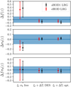 |
Fig. 10 Comparison between a fit to the multipoles ξℓ only (left) and a fit to the combined ξℓ + ∆Σ data vector. We present constraints for the scale cuts used for γt in the DES y3 analysis (Krause et al. 2021), rmin = 6 h−1 Mpc, and for the optimal configuration determined in this work, rmin = 3 h−1 Mpc. |
Acknowledgements
The authors thank the referee for the useful comments that considerably improved the quality of this work. RP is supported by a DIM-ACAV+ fellowship from Region Ile-de-France. SC acknowledges financial support from Fondation MERAC and by the SPHERES grant ANR-18-CE31- 0009 of the French Agence Nationale de la Recherche. In addition to the packages already quoted in the main text, we also acknowledge the use of numpy (Harris et al. 2020) and scipy (Virtanen et al. 2020). Plots were made with matplotlib Hunter (2007) while corner plots were made with pygtc Bocquet & Carter (2016).
Appendix A Robustness of the analysis
In our main analysis, we fix the number density in the simulation box to be twice the mean number density of LRG, where  . This choice was motivated by the fact that increasing the number density provides higher S/N measurements such that averaging over ten realisations is enough to get robust likelihood estimates. This is particularly important for numerical speed, as we do not use any emulator to compute ΔΣ. In Fig. A.1, we present the posterior distributions, this time fixing the number density of galaxy in the box to 4 times the number density of LRG. As we can see, the environmental dependence on halo occupation is unchanged.
Additionally, we modified the NFW radial profile as done in Avila et al. (2020). We introduce an additional nuisance parameter s, and we modify the concentration of each halo by cnew = s × c. We allowed s to vary in the range [0.5, 1.5]. We present the result in Fig. A.2. This additional degree of freedom does not introduce significant change in the environmental dependence of halo occupation. Additionally, we can see that the data seems to favour an NFW profile.
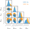 |
Fig. A.1 Full posterior distributions of the assembly bias and environmental parameters in our baseline configuration. We also present our result with a different number density from the one defined in the main text. The dependence of halo occupation on the environment is unchanged. |
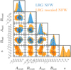 |
Fig. A.2 Full posterior distributions of the assembly bias and environmental parameters in our baseline configuration. We also present our result with a modified NFW profile. The dependence of halo occupation on the environment is unchanged. |
Appendix B Additional parameters
We present in Fig. B.1 the normalised distribution in the range [1,1] of internal (concentration and ellipticity) and external (local density and local shear) halo properties on the left and right panel respectively. We present in Fig. B.2 the relation between the two different local density estimators described in this work.
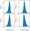 |
Fig. B.1 Distribution of internal and external halo properties as defined in Sect. 3.2. The left panels present the distribution of concentration (c) and ellipticity (e), while the right panels present the local density (d) and local shear (s). |
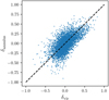 |
Fig. B.2 Comparison between the local density estimated on a mesh with a Gaussian filter of size R = 2.25 rvir and the local density estimated by summing halo and sub-halo masses around rvir and 5 h−1 Mpc. The dashed line corresponds to δvir = δannulus . |
Appendix C Posterior of the luminous red galaxies halo occupation distribution
We present here the full posterior contours in Fig. C.1 in the fiducial configuration. Additionally, we present in Table C.1 the posterior distributions for all configurations presented in Sect. 4.3.
We only present Mmin for the posterior distributions presented in Fig. 4 to save computational time, as Mmin is not a free parameter and is computed for each point of the chain given Eq. (7). In addition, for completeness, we also present the full posterior contours.
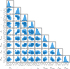 |
Fig. C.1 Full posterior distribution of the LRG-extended HOD, including the assembly bias parameters in the fiducial configuration. |
Result of the Gaussian process emulating the likelihood function after 4000 iterations for the eBOSS LRG sample.
References
- Abbott, T. M. C., Aguena, M., Alarcon, A., et al. 2022, Phys. Rev. D, 105, 023520 [CrossRef] [Google Scholar]
- Alam, S., Peacock, J. A., Kraljic, K., Ross, A. J., & Comparat, J. 2020, MNRAS, 497, 581 [NASA ADS] [CrossRef] [Google Scholar]
- Alam, S., de Mattia, A., Tamone, A., et al. 2021, MNRAS, 504, 4667 [NASA ADS] [CrossRef] [Google Scholar]
- Alcock, C., & Paczynski, B. 1979, Nature, 281, 358 [NASA ADS] [CrossRef] [Google Scholar]
- Allgood, B., Flores, R. A., Primack, J. R., et al. 2006, MNRAS, 367, 1781 [NASA ADS] [CrossRef] [Google Scholar]
- Amodeo, S., Battaglia, N., Schaan, E., et al. 2021, Phys. Rev. D, 103, 063514 [NASA ADS] [CrossRef] [Google Scholar]
- Artale, M. C., Zehavi, I., Contreras, S., & Norberg, P. 2018, MNRAS, 480, 3978 [NASA ADS] [CrossRef] [Google Scholar]
- Assassi, V., Baumann, D., Green, D., & Zaldarriaga, M. 2014, J. Cosmology Astropart. Phys., 2014, 056 [CrossRef] [Google Scholar]
- Avila, S., Gonzalez-Perez, V., Mohammad, F. G., et al. 2020, MNRAS, 499, 5486 [NASA ADS] [CrossRef] [Google Scholar]
- Baldauf, T., Smith, R. E., Seljak, U. c. v., & Mandelbaum, R. 2010, Phys. Rev. D, 81, 063531 [NASA ADS] [CrossRef] [Google Scholar]
- Bautista, J. E., Paviot, R., Vargas Magaña, M., et al. 2021, MNRAS, 500, 736 [Google Scholar]
- Behroozi, P. S., Wechsler, R. H., & Wu, H.-Y. 2013, ApJ, 762, 109 [NASA ADS] [CrossRef] [Google Scholar]
- Bel, J., Pezzotta, A., Carbone, C., Sefusatti, E., & Guzzo, L. 2019, A&A, 622, A109 [NASA ADS] [CrossRef] [EDP Sciences] [Google Scholar]
- Berlind, A. A., & Weinberg, D. H. 2002, ApJ, 575, 587 [Google Scholar]
- Bocquet, S., & Carter, F. W. 2016, J. Open Source Softw., 1, 46 [NASA ADS] [CrossRef] [Google Scholar]
- Bose, S., Eisenstein, D. J., Hernquist, L., et al. 2019, MNRAS, 490, 5693 [CrossRef] [Google Scholar]
- Chaves-Montero, J., Angulo, R. E., Schaye, J., et al. 2016, MNRAS, 460, 3100 [NASA ADS] [CrossRef] [Google Scholar]
- Chaves-Montero, J., Angulo, R. E., & Contreras, S. 2023, MNRAS, 521, 937 [Google Scholar]
- Conroy, C., Wechsler, R. H., & Kravtsov, A. V. 2006, ApJ, 647, 201 [Google Scholar]
- Contreras, S., Angulo, R. E., Chaves-Montero, J., White, S. D. M., & Aricò, G. 2023a, MNRAS, 520, 489 [Google Scholar]
- Contreras, S., Chaves-Montero, J., & Angulo, R. E. 2023b, MNRAS, 525, 3149 [NASA ADS] [CrossRef] [Google Scholar]
- Croton, D. J., Gao, L., & White, S. D. M. 2007, MNRAS, 374, 1303 [Google Scholar]
- Dalal, N., White, M., Bond, J. R., & Shirokov, A. 2008, ApJ, 687, 12 [NASA ADS] [CrossRef] [Google Scholar]
- Dark Energy Survey Collaboration (Abbott, T., et al.) 2016, MNRAS, 460, 1270 [Google Scholar]
- Dawson, K. S., Schlegel, D. J., Ahn, C. P., et al. 2013, AJ, 145, 10 [Google Scholar]
- Dawson, K. S., Kneib, J.-P., Percival, W. J., et al. 2016, AJ, 151, 44 [Google Scholar]
- de la Torre, S., Jullo, E., Giocoli, C., et al. 2017, A&A, 608, A44 [NASA ADS] [CrossRef] [EDP Sciences] [Google Scholar]
- de Mattia, A., Ruhlmann-Kleider, V., Raichoor, A., et al. 2021, MNRAS, 501, 5616 [NASA ADS] [Google Scholar]
- De Vicente, J., Sánchez, E., & Sevilla-Noarbe, I. 2016, MNRAS, 459, 3078 [NASA ADS] [CrossRef] [Google Scholar]
- Delgado, A. M., Wadekar, D., Hadzhiyska, B., et al. 2022, MNRAS, 515, 2733 [NASA ADS] [CrossRef] [Google Scholar]
- DESI Collaboration 2016, arXiv e-prints [arXiv:1611.00036] [Google Scholar]
- Euclid Collaboration (Mellier, Y., et al.) 2024, A&A, in press, https://doi.org/10.1051/0004-6361/202450810 [Google Scholar]
- Feldman, H. A., Kaiser, N., & Peacock, J. A. 1994, ApJ, 426, 23 [Google Scholar]
- Foreman-Mackey, D., et al. 2013, PASP, 125, 306 [NASA ADS] [CrossRef] [Google Scholar]
- Gao, L., & White, S. D. M. 2007, MNRAS, 377, L5 [NASA ADS] [CrossRef] [Google Scholar]
- Gatti, M., Sheldon, E., Amon, A., et al. 2021, MNRAS, 504, 4312 [NASA ADS] [CrossRef] [Google Scholar]
- Gil-Marín, H., Bautista, J. E., Paviot, R., et al. 2020, MNRAS, 498, 2492 [Google Scholar]
- Gonzalez-Perez, V., Comparat, J., Norberg, P., et al. 2018, MNRAS, 474, 4024 [NASA ADS] [CrossRef] [Google Scholar]
- Gonzalez-Perez, V., Cui, W., Contreras, S., et al. 2020, MNRAS, 498, 1852 [NASA ADS] [CrossRef] [Google Scholar]
- Górski, K. M., Hivon, E., Banday, A. J., et al. 2005, ApJ, 622, 759 [Google Scholar]
- Gouin, C., Gavazzi, R., Pichon, C., et al. 2019, A&A, 626, A72 [NASA ADS] [CrossRef] [EDP Sciences] [Google Scholar]
- Grieb, J. N., Sánchez, A. G., Salazar-Albornoz, S., & Dalla Vecchia, C. 2016, MNRAS, 457, 1577 [NASA ADS] [CrossRef] [Google Scholar]
- Guzik, J., & Seljak, U. 2001, MNRAS, 321, 439 [Google Scholar]
- Hadzhiyska, B., Bose, S., Eisenstein, D., Hernquist, L., & Spergel, D. N. 2020, MNRAS, 493, 5506 [NASA ADS] [CrossRef] [Google Scholar]
- Hadzhiyska, B., Tacchella, S., Bose, S., & Eisenstein, D. J. 2021, MNRAS, 502, 3599 [NASA ADS] [CrossRef] [Google Scholar]
- Hadzhiyska, B., Eisenstein, D., Hernquist, L., et al. 2023a, MNRAS, 524, 2507 [NASA ADS] [CrossRef] [Google Scholar]
- Hadzhiyska, B., Hernquist, L., Eisenstein, D., et al. 2023b, MNRAS, 524, 2524 [NASA ADS] [CrossRef] [Google Scholar]
- Hahn, C., Lemos, P., Parker, L., et al. 2023, arXiv e-prints [arXiv:2310.15246] [Google Scholar]
- Hamilton, A. J. S. 2000, MNRAS, 312, 257 [NASA ADS] [CrossRef] [Google Scholar]
- Harris, C. R., Millman, K. J., van der Walt, S. J., et al. 2020, Nature, 585, 357 [NASA ADS] [CrossRef] [Google Scholar]
- Hunter, J. D. 2007, Comput. Sci. Eng., 9, 90 [NASA ADS] [CrossRef] [Google Scholar]
- Ishiyama, T., Fukushige, T., & Makino, J. 2009, PASJ, 61, 1319 [NASA ADS] [CrossRef] [Google Scholar]
- Ishiyama, T., Nitadori, K., & Makino, J. 2012, arXiv e-prints [arXiv:1211.4406] [Google Scholar]
- Ishiyama, T., Prada, F., Klypin, A. A., et al. 2021, MNRAS, 506, 4210 [NASA ADS] [CrossRef] [Google Scholar]
- Jeffrey, N., Whiteway, L., Gatti, M., et al. 2024, arXiv e-prints [arXiv:2403.02314] [Google Scholar]
- Jullo, E., de la Torre, S., Cousinou, M. C., et al. 2019, A&A, 627, A137 [NASA ADS] [CrossRef] [EDP Sciences] [Google Scholar]
- Kaiser, N. 1984, ApJ, 284, L9 [NASA ADS] [CrossRef] [Google Scholar]
- Kaiser, N. 1987, MNRAS, 227, 1 [Google Scholar]
- Krause, E., Fang, X., Pandey, S., et al. 2021, arXiv e-prints [arXiv:2105.13548] [Google Scholar]
- Landy, S. D., & Szalay, A. S. 1993, ApJ, 412, 64 [Google Scholar]
- Lange, J., & Huang, S. 2022, dsigma: Galaxy-galaxy lensing Python package, Astrophysics Source Code Library [record ascl:2204.006] [Google Scholar]
- Lange, J. U. 2023, MNRAS, 525, 3181 [NASA ADS] [CrossRef] [Google Scholar]
- Leauthaud, A., Saito, S., Hilbert, S., et al. 2017, MNRAS, 467, 3024 [Google Scholar]
- Lewis, A., & Challinor, A. 2011, CAMB: Code for Anisotropies in the Microwave Background, Astrophysics Source Code Library [record ascl:1102.026] [Google Scholar]
- Limber, D. N. 1953, ApJ, 117, 134 [NASA ADS] [CrossRef] [Google Scholar]
- Marian, L., Smith, R. E., & Angulo, R. E. 2015, MNRAS, 451, 1418 [NASA ADS] [CrossRef] [Google Scholar]
- McDonald, P., & Roy, A. 2009, J. Cosmology Astropart. Phys., 2009, 020 [CrossRef] [Google Scholar]
- Mead, A. J., Brieden, S., Tröster, T., & Heymans, C. 2021, MNRAS, 502, 1401 [Google Scholar]
- Miyatake, H., More, S., Mandelbaum, R., et al. 2015, ApJ, 806, 1 [NASA ADS] [CrossRef] [Google Scholar]
- Mohammad, F. G., Percival, W. J., Seo, H.-J., et al. 2020, MNRAS, 498, 128 [Google Scholar]
- Musso, M., Cadiou, C., Pichon, C., et al. 2018, MNRAS, 476, 4877 [Google Scholar]
- Myles, J., Alarcon, A., Amon, A., et al. 2021, MNRAS, 505, 4249 [NASA ADS] [CrossRef] [Google Scholar]
- Navarro, J. F., Frenk, C. S., & White, S. D. M. 1996, ApJ, 462, 563 [Google Scholar]
- Nishimichi, T., Bernardeau, F., & Taruya, A. 2017, Phys. Rev. D, 96, 123515 [NASA ADS] [CrossRef] [Google Scholar]
- Paranjape, A., Hahn, O., & Sheth, R. K. 2018, MNRAS, 476, 3631 [NASA ADS] [CrossRef] [Google Scholar]
- Paviot, R., de la Torre, S., de Mattia, A., et al. 2022, MNRAS, 512, 1341 [NASA ADS] [CrossRef] [Google Scholar]
- Planck Collaboration XIII. 2016, A&A, 594, A13 [NASA ADS] [CrossRef] [EDP Sciences] [Google Scholar]
- Reddick, R. M., Wechsler, R. H., Tinker, J. L., & Behroozi, P. S. 2013, ApJ, 771, 30 [Google Scholar]
- Rocher, A., Ruhlmann-Kleider, V., Burtin, E., & de Mattia, A. 2023a, J. Cosmology Astropart. Phys., 2023, 033 [CrossRef] [Google Scholar]
- Rocher, A., Ruhlmann-Kleider, V., Burtin, E., et al. 2023b, J. Cosmology Astropart. Phys., 2023, 016 [CrossRef] [Google Scholar]
- Ross, A. J., Bautista, J., Tojeiro, R., et al. 2020, MNRAS, 498, 2354 [NASA ADS] [CrossRef] [Google Scholar]
- Rossi, G., Choi, P. D., Moon, J., et al. 2021, MNRAS, 505, 377 [NASA ADS] [CrossRef] [Google Scholar]
- Saito, S., Baldauf, T., Vlah, Z., et al. 2014, Phys. Rev. D, 90, 123522 [NASA ADS] [CrossRef] [Google Scholar]
- Sevilla-Noarbe, I., Bechtol, K., Carrasco Kind, M., et al. 2021, ApJS, 254, 24 [NASA ADS] [CrossRef] [Google Scholar]
- Simonović, M., Baldauf, T., Zaldarriaga, M., Carrasco, J. J., & Kollmeier, J. A. 2018, J. Cosmology Astropart. Phys., 2018, 030 [CrossRef] [Google Scholar]
- Singh, S., Mandelbaum, R., Seljak, U., Slosar, A., & Vazquez Gonzalez, J. 2017, MNRAS, 471, 3827 [Google Scholar]
- Sinha, M., & Garrison, L. H. 2020, MNRAS, 491, 3022 [Google Scholar]
- Tamone, A., Raichoor, A., Zhao, C., et al. 2020, MNRAS, 499, 5527 [Google Scholar]
- Taruya, A., Nishimichi, T., & Saito, S. 2010, Phys. Rev. D, 82, 063522 [NASA ADS] [CrossRef] [Google Scholar]
- Vale, A., & Ostriker, J. P. 2006, MNRAS, 371, 1173 [NASA ADS] [CrossRef] [Google Scholar]
- van den Bosch, F. C., More, S., Cacciato, M., Mo, H., & Yang, X. 2013, MNRAS, 430, 725 [NASA ADS] [CrossRef] [Google Scholar]
- Virtanen, P., Gommers, R., Oliphant, T. E., et al. 2020, Nature Methods, 17, 261 [CrossRef] [Google Scholar]
- von Wietersheim-Kramsta, M., Lin, K., Tessore, N., et al. 2024, A&A, submitted [Google Scholar]
- Wechsler, R. H., Bullock, J. S., Primack, J. R., Kravtsov, A. V., & Dekel, A. 2002, ApJ, 568, 52 [NASA ADS] [CrossRef] [Google Scholar]
- White, M., Blanton, M., Bolton, A., et al. 2011, ApJ, 728, 126 [NASA ADS] [CrossRef] [Google Scholar]
- White, S. D. M., & Rees, M. J. 1978, MNRAS, 183, 341 [Google Scholar]
- Xu, X., Zehavi, I., & Contreras, S. 2021, MNRAS, 502, 3242 [NASA ADS] [CrossRef] [Google Scholar]
- York, D. G., Adelman, J., Anderson, John E.J., et al. 2000, AJ, 120, 1579 [NASA ADS] [CrossRef] [Google Scholar]
- Yuan, S., Hadzhiyska, B., Bose, S., Eisenstein, D. J., & Guo, H. 2021, MNRAS, 502, 3582 [NASA ADS] [CrossRef] [Google Scholar]
- Yuan, S., Garrison, L. H., Hadzhiyska, B., Bose, S., & Eisenstein, D. J. 2022, MNRAS, 510, 3301 [NASA ADS] [CrossRef] [Google Scholar]
- Zehavi, I., Contreras, S., Padilla, N., et al. 2018, ApJ, 853, 84 [NASA ADS] [CrossRef] [Google Scholar]
- Zhai, Z., Tinker, J. L., Hahn, C., et al. 2017, ApJ, 848, 76 [NASA ADS] [CrossRef] [Google Scholar]
- Zheng, Z., Berlind, A. A., Weinberg, D. H., et al. 2005, ApJ, 633, 791 [NASA ADS] [CrossRef] [Google Scholar]
- Zheng, Z., Coil, A. L., & Zehavi, I. 2007, ApJ, 667, 760 [Google Scholar]
We refer to it as an LRG sample for simplicity. Catalogues can be found at https://data.sdss.org/sas/dr17/eboss/lss/catalogs/DR16/
These values were computed with Healpix (Górski et al. 2005) with NSIDE = 512.
Throughout this paper, the logarithm notation refers to the decimal logarithm unless specified otherwise.
We drop the subscripts for simplicity in the following sections.
A top hat filter of size R is equivalent to a Gaussian filter of size  (see Paranjape et al. 2018).
This is the maximum number of particles that can be extracted from the simulation.
Wrapped around cosmoprimo https://cosmoprimo.readthedocs.io/en/latest/index.html
All Tables
Best-fit parameters of the LRG HOD for all configurations defined in the main text.
Result of the Gaussian process emulating the likelihood function after 4000 iterations for the eBOSS LRG sample.
All Figures
|
Fig. 1 Galaxy number density (left panel) and footprint (right panel) of the LRG sample (green), the ELG sample (blue), and the DES y3 GOLD catalogue (red). The n(z) of DES corresponds to the concatenation of the n(z) on each tomographic bin (Myles et al. 2021). It has been sub-sampled by a factor 20 for clarity. On the right panel, we present the DES footprint with a cut below a declination of −12. |
| In the text | |
|
Fig. 2 Best-fit HOD models for LRG (top) and ELG (bottom). The subscript ‘s/e’ denotes the standard and extended HOD model. The extended model here corresponds to our fiducial configuration, where the concentration and an annular definition of δ are used as additional parameters. The points with error bars correspond to the measured wp (left) and the ∆Σ (right) signals. The blue lines (sHOD1) correspond to a fit to the projected correlation function wp only, while the green (SHOD2) and orange lines (eHOD) correspond to standard and extended HOD fits including the measurement of ∆Σ in the fitting pipeline. The extended HOD model provides a good description of both the clustering and lensing signal. We did not perform any standard HOD fit to the combined wp + ∆Σ vector for ELGs (sHOD2), as the standard HOD fit to wp only already agrees well with the ∆Σ measurement. |
| In the text | |
|
Fig. 3 Difference between the observed galaxy-galaxy lensing signal (points with error bars) of eBOSS LRGs with the prediction of a standard HOD (sHOD) determined by fitting the projected correlation function wp only. The continuous line in blue represents an sHOD fit to wp + ΔΣ, while the orange line corresponds to the extended HOD model. |
| In the text | |
|
Fig. 4 Posterior contours of the sHOD1 (in blue), sHOD2 (in orange), and eHOD (in green) in our baseline configuration (including concentration and annular density as additional parameters) for the LRG sample. One can observe that the extra parameters contained in the eHOD model have a strong impact on the posterior distributions. |
| In the text | |
|
Fig. 5 Posterior contours of the assembly bias and environmental parameters in our baseline configuration (see Sect. 4.1). For the LRG, the negative value of Bcent, detected at 3σ, indicates that LRG centrals most likely occupy a dense environment. A negative value of Asat at the 1σ level indicates that satellite galaxies could be preferentially located in more concentrated halos than average. For the ELGs, all parameters are consistent with zero at the 1σ level, suggesting that ELGs do not exhibit significant assembly bias or environmental dependencies. |
| In the text | |
|
Fig. 6 Posterior contours for the sHOD (in blue) and eHOD (in orange) models for the ELG sample. Taking into account assembly bias parameters has little impact on halo occupation. |
| In the text | |
|
Fig. 7 Result for different combinations of assembly bias (concentration and shape) and local environments (density and shear) parameters. Top panels present the measurements, while the bottom panels show the relative differences. Nearly all the models provide similar best-fitting clustering predictions, lensing predictions, and goodness of fit results except the shear measured with a Gaussian Kernel of size 2.25 h−1 Mpc, which has a slightly worse goodness of fit. |
| In the text | |
|
Fig. 8 Results from the cosmological fit. Circle points with error bars correspond to the fit of the LRG sample at redshift ɀ = 0.70 populated with the standard and extended HOD framework, while the triangles correspond to the fit of ELGs at redshift ɀ = 0.86. The value of f and σ8 for LRGs (ELGs) are 0.814 (0.849) and 0.570 (0.529) at the redshift ɀ = 0.70(0.86). Values in parentheses correspond to the minimum scale used in the fit in megaparsec per h. The shaded area corresponds to a 10% variation around the fiducial value of each parameter. |
| In the text | |
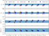 |
Fig. 9 Same as Fig. 8 but this time considering the annular excess surface density Υ instead. |
| In the text | |
|
Fig. 10 Comparison between a fit to the multipoles ξℓ only (left) and a fit to the combined ξℓ + ∆Σ data vector. We present constraints for the scale cuts used for γt in the DES y3 analysis (Krause et al. 2021), rmin = 6 h−1 Mpc, and for the optimal configuration determined in this work, rmin = 3 h−1 Mpc. |
| In the text | |
|
Fig. A.1 Full posterior distributions of the assembly bias and environmental parameters in our baseline configuration. We also present our result with a different number density from the one defined in the main text. The dependence of halo occupation on the environment is unchanged. |
| In the text | |
|
Fig. A.2 Full posterior distributions of the assembly bias and environmental parameters in our baseline configuration. We also present our result with a modified NFW profile. The dependence of halo occupation on the environment is unchanged. |
| In the text | |
|
Fig. B.1 Distribution of internal and external halo properties as defined in Sect. 3.2. The left panels present the distribution of concentration (c) and ellipticity (e), while the right panels present the local density (d) and local shear (s). |
| In the text | |
|
Fig. B.2 Comparison between the local density estimated on a mesh with a Gaussian filter of size R = 2.25 rvir and the local density estimated by summing halo and sub-halo masses around rvir and 5 h−1 Mpc. The dashed line corresponds to δvir = δannulus . |
| In the text | |
|
Fig. C.1 Full posterior distribution of the LRG-extended HOD, including the assembly bias parameters in the fiducial configuration. |
| In the text | |
Current usage metrics show cumulative count of Article Views (full-text article views including HTML views, PDF and ePub downloads, according to the available data) and Abstracts Views on Vision4Press platform.
Data correspond to usage on the plateform after 2015. The current usage metrics is available 48-96 hours after online publication and is updated daily on week days.
Initial download of the metrics may take a while.