| Issue |
A&A
Volume 699, July 2025
|
|
|---|---|---|
| Article Number | A201 | |
| Number of page(s) | 18 | |
| Section | Cosmology (including clusters of galaxies) | |
| DOI | https://doi.org/10.1051/0004-6361/202453442 | |
| Published online | 07 July 2025 | |
UNIONS: A direct measurement of intrinsic alignment with BOSS/eBOSS spectroscopy
1
Université Paris-Saclay, Université Paris Cité, CEA, CNRS, AIM, 91191 Gif-sur-Yvette, France
2
Dipartimento di Fisica – Sezione di Astronomia, Università di Trieste, Via Tiepolo 11, 34131 Trieste, Italy
3
INAF-Osservatorio Astronomico di Trieste, Via G. B. Tiepolo 11, 34143 Trieste, Italy
4
Lawrence Berkeley National Laboratory, 1 Cyclotron Road, Berkeley, CA 94720, USA
5
CAS Key Laboratory for Research in Galaxies and Cosmology, Department of Astronomy, University of Science and Technology of China, Hefei, Anhui 230026, China
6
School of Astronomy and Space Science, University of Science and Technology of China, Hefei 230026, China
7
European Space Agency/ESTEC, Keplerlaan 1, 2201 AZ Noordwijk, The Netherlands
8
Institute for Astronomy, University of Hawaii, 2680 Woodlawn Drive, Honolulu, HI 96822, USA
9
NRC Herzberg Astronomy & Astrophysics, 5071 West Saanich Road, British Columbia V9E2E7, Canada
10
Ruhr University Bochum, Faculty of Physics and Astronomy, Astronomical Institute (AIRUB), German Centre for Cosmological Lensing, 44780 Bochum, Germany
11
Department of Physics and Astronomy, University of Waterloo, Waterloo, ON N2L 3G1, Canada
12
Waterloo Centre for Astrophysics, University of Waterloo, Waterloo, ON N2L 3G1, Canada
13
Perimeter Institute for Theoretical Physics, Waterloo ON N2L 2Y5, Canada
14
Department of Physics and Astronomy, University of British Columbia, Vancouver, V6T1Z1 BC, Canada
⋆ Corresponding author: This email address is being protected from spambots. You need JavaScript enabled to view it.
Received:
13
December
2024
Accepted:
14
April
2025
Abstract
Context. During their formation, galaxies are subject to tidal forces, which create correlations between their shapes and the large-scale structure of the Universe, known as intrinsic alignment. This alignment is a source of contamination for cosmic-shear measurements as we need to disentangle correlations induced by external lensing effects from those intrinsically present in galaxies.
Aims. We constrained the amplitude of intrinsic alignment and test models by making use of the overlap between the Ultraviolet Near-Infrared Optical Northern Survey (UNIONS) covering 3500 deg2 and spectroscopic data from the Baryon Oscillation Spectroscopic Survey (BOSS/eBOSS). By comparing our results to measurements from other lensing surveys on the same spectroscopic tracers, we can test the reliability of these estimates.
Methods. We measured projected correlation functions between positions and ellipticities, which we modelled with perturbation theory to constrain the commonly used non-linear alignment model and its higher order expansion. We computed an analytical covariance matrix and validated it using jackknife estimates.
Results. Using the non-linear alignment model, we obtained a 13σ detection with CMASS galaxies, a 3σ detection with LRGs, and a detection compatible with the null hypothesis for ELGs. We tested the tidal alignment and tidal torque model. This is a higher order alignment model that we found to be in good agreement with the non-linear alignment prediction and for which we were able to constrain the second-order parameters. We demonstrate the strong scaling of our intrinsic alignment amplitude with luminosity. We also demonstrate that the UNIONS sample is robust against systematic contributions, particularly concerning the point spread function (PSF) biases. We reached a reasonable agreement when comparing our measurements to other lensing samples for the same spectroscopic samples. We take this agreement as an indication that direct measurements of intrinsic alignment are mature for stage IV priors.
Key words: cosmological parameters / large-scale structure of Universe
© The Authors 2025
 Open Access article, published by EDP Sciences, under the terms of the Creative Commons Attribution License (https://creativecommons.org/licenses/by/4.0), which permits unrestricted use, distribution, and reproduction in any medium, provided the original work is properly cited.
This article is published in open access under the Subscribe to Open model. This email address is being protected from spambots. You need JavaScript enabled to view it. to support open access publication.
1. Introduction
In recent years, cosmic shear measurements have demonstrated a capacity to constrain the dark-matter distribution on cosmological scales (Dark Energy Survey and Kilo-Degree Survey Collaboration 2023; More et al. 2023). Over the coming decade, they represent a key probe in determining our Universe’s cosmological scenario at later times and to gain insights into the nature of dark energy and dark matter at lower and intermediate redshift. Weak lensing is one of the primary cosmological probes for a number of upcoming surveys, including Euclid (Euclid Collaboration: Mellier et al. 2025), Vera Rubin Observatory Legacy Survey of Space and Time (LSST; Ivezić et al. 2019), and Nancy Grace Roman Space Telescope (Roman; Eifler et al. 2021). The cosmic shear signal is estimated by averaging over the shape of background galaxies, which are coherently deformed as their light travels through the large scale structures. By studying the correlations between the shapes of neighbouring galaxies, we can infer the foreground distribution of matter, particularly dark matter. In the coming decade, unprecedented statistical power will be reached by modern weak lensing experiments, which are poised to observe billions of galaxies. This increase in statistical power means that systematic contributions, which had previously been of lesser importance, can lead to important biases if they are not accounted for. These systematic contributions can be broadly split into two categories: biases at the measurement level and biases at the modelling level. In the latter, three sources of biases are particularly critical: baryonic feedback, a non-linear effect that suppresses mode fluctuations in the range of k ∼ [0.1, 10] Mpc/h, photometric-redshift biases caused by a poor estimation of the galaxies redshift distribution, and galaxy intrinsic alignment; the latter is due to the fact that galaxy orientations are not uniformly distributed on the sky, but correlated with their environments. For a review, we refer to Mandelbaum (2018).
It was shown in Catelan et al. (2001) and Crittenden et al. (2001) that tidal forces arising from the density field have the potential to produce coherent orientations in neighboring galaxies, which can pose a challenge for cosmic shear. Specifically, the difficulty lies in disentangling the correlations induced directly on the galaxy shapes by the tidal forces from those caused by the shearing of the light profile due to gravitational lensing. The effects of tidal forces on the orientation of galaxies have been described in Catelan et al. (2001) and in Mackey et al. (2002). For a review and visual explanations, we refer to Joachimi et al. (2015), Lamman et al. (2024).
To mitigate the intrinsic alignment, various solutions have been proposed. To remove the intrinsic alignment from the cosmic-shear signal, two main methods exist: ‘down-weighting’ (King & Schneider 2002) and ‘nulling’ (Heavens & Joachimi 2011). Down-weighting consists of suppressing the correlation between pairs of galaxies that are close in redshift and subject to intrinsic alignment. This is achieved by applying a Gaussian weighting factor in the correlation function estimator to suppress the contributions from close pairs. This weighting factor has a variance reflecting the photometric redshift uncertainty, which implies that imprecise photometric redshifts will lead to a large loss of statistical power, as many pairs are suppressed. The concept of ‘nulling’ uses the specific dependency of the lensing kernel on the comoving distance to suppress any combination of bins that might be too sensitive to the interplay between shear and intrinsic alignment. For a review, we refer to Kirk et al. (2015).
These methods, however, have been shown to strongly reduce the statistical power of a weak lensing survey and to be very dependent on precise photometric redshifts. The approach taken in recent stage-III cosmic shear surveys has therefore consisted of the joint modelling of the weak lensing and the intrinsic alignment signal. Two main models have been applied: the non-linear alignment model (NLA) and its higher-order expansion, the tidal alignment and tidal torque model (TATT). These models are described in Sects. 4.2.1 and 4.2.2. They are theoretically motivated, but the physical range of their validity remains an open question. In particular, Bakx et al. (2023) recently showed that the NLA (TATT) prediction of the alignment of subhaloes in the DarkQuest simulation is only able to describe correlations on modes smaller than k ≤ 0.08 h/Mpc (k ≤ 0.15 h/Mpc). This shortcoming has motivated the inclusion of even higher order terms in the effective field theory approach. With eight free parameters (Vlah et al. 2020), this model is harder to constrain than the NLA and TATT models, which have one and three parameters, respectively, when the redshift and luminosity dependencies are fixed. A similar EFT approach can be found in Chen & Kokron (2024). We note that while these theoretically motivated models are essential in the prediction of the weak lensing correlation functions, they are also used to add intrinsic alignment to convergence maps used in simulation-based approaches, which require the full-field information (Harnois-Déraps et al. 2021; Kacprzak et al. 2023; Jeffrey et al. 2024). Similarly, this model has been applied in a direct inference of the galaxies’ alignment with the tidal field, which is itself inferred from SDSS spectroscopic tracers (Tsaprazi et al. 2022). Other models based on the halo model (Schneider & Bridle 2010; Fortuna et al. 2021a) achieve higher accuracy at smaller scales by incorporating an intrinsic ellipticity field within each halo. These models predict distinct effects on central and satellite galaxies, with probability distributions derived from halo-occupation distribution models based on an NFW profile and dependent on halo mass.
To properly characterise the intrinsic alignment, various hydrodynamical simulations have been used (Chisari et al. 2015; Samuroff et al. 2021). While they offer a picture that is broadly consistent with observations, no precise calibration has been reached from these various simulations, as the selection of galaxies and their mapping to phenomenological properties remains challenging. In Tenneti et al. (2016), it was shown that the choice of elliptical galaxies can produce drastic changes, as the ellipticity-density correlation can go from positively to negatively correlated depending on the simulation. A more novel route to calibrating the intrinsic alignment, which makes use of the power of N-body simulations to describe the large-scale structure of the Universe, is to add galaxies empirically. This is performed by drawing misalignment angles from probability distribution functions, which are calibrated on observations or hydrodynamical simulations and draw central and satellite galaxy populations from a halo occupation distribution model (Hoffmann et al. 2022; Van Alfen et al. 2024).
In parallel, and complementary to the simulation efforts, many studies have tried to constrain intrinsic alignment models by direct measurements, which require precise redshift information to disentangle lensing contributions from intrinsic alignment. They have shown a strong intrinsic alignment between red galaxies at scales relevant for the two-halo term (i.e. ∼6 − 150 Mpc) outside the one-halo regime (Joachimi et al. 2013; Singh et al. 2015, hereafter Si15; Johnston et al. 2019; Fortuna et al. 2021b; Samuroff et al. 2018). For red galaxies, the intrinsic alignment was shown to depend on luminosity following a broken power law, (Fortuna et al. 2021a; Samuroff et al. 2023, hereafter Sa23). For blue spiral galaxies, direct measurements tend to prefer an absence of intrinsic alignment (Mandelbaum et al. 2011; Johnston et al. 2019; Tonegawa et al. 2024; Sa23). The alignment between blue and red samples was adequately measured in Johnston et al. (2019), was made possible by the very densely sampled and complete spectroscopic galaxy and mass assembly survey (GAMA, Hopkins et al. 2013), overlapping with the KiDS dataset (Giblin et al. 2021). Very recently, McCullough et al. (2024) showed a strong difference in cosmological parameter estimation from cosmic shear when splitting the DES Y3 in red and blue galaxy samples. This difference was attributed to the varying sensitivities of these samples to the intrinsic alignment models.
This work contributes to the challenge of propagating intrinsic alignment measurements into a sensible prior for stage-IV surveys. This task is complicated by a few subtleties affecting observations and the resulting amplitude of intrinsic alignment. One such effect is the dependence of the intrinsic alignment amplitude on the shape measurement method: as tidal forces act stronger on the outskirts of galaxies, these extended regions are more affected by intrinsic alignment than the central part. This was first observed in Singh & Mandelbaum (2016), who found a 40% amplitude difference between the re-Gaussianisation, isophotal, and de-Vaucouleurs shape measurement methods. While these three shape measurement methods are less frequently used in stage-III surveys, a recent work (MacMahon-Gellér & Leonard 2024) showed how this effect can be used to gain information on intrinsic alignment effects. In this work, the authors applied the multi-estimator method (MEM) described in Leonard et al. (2018), which uses the different deformations in isophotes between intrinsic alignment and cosmic shear to disentangle the two effects. They found that a 40% difference in the intrinsic alignment amplitude is required for a 1σ detection in LSST Year 1 data. In Georgiou et al. (2019a,b), a strong change in IA amplitude was shown by varying the weight function of the shape measurement. In addition Georgiou et al. (2019a) noted a chromatic effect in intrinsic alignment by changing the photometric band in which the galaxy shape is measured.
In this work, we applied the projected two-point correlation function, but other estimators have recently been developed. In Linke et al. (2024), a three-point correlation function with LOWZ data was found to be in good agreement with the two-point correlation functions, promising better constraining power for future surveys. Another important avenue is the three-dimensional measurement in Fourier space, known as the Yamamoto estimator (Yamamoto et al. 2006). It was initially used by the galaxy clustering community, but it has been applied successfully to constrain intrinsic alignment (Kurita et al. 2021; Kurita & Takada 2023). Similarly, Singh et al. (2024) showed that including real-space multipoles can also help in reaching tighter constraints.
While intrinsic alignment is a treated as a source of contamination with respect to to weak lensing measurements, it is also a cosmological probe in its own right. Examples include the detection of baryon acoustic oscillations (BAOs) in the intrinsic-alignment correlation functions (van Dompseler et al. 2023; Xu et al. 2023a) and constraints on primordial non-Gaussianities (Schmidt et al. 2015; Chisari et al. 2016; Kurita & Takada 2023).
In this work, we used the UNIONS imaging survey together with BOSS/eBOSS spectroscopic galaxies to measure the intrinsic alignment. We compared our measurements to other samples by investigating the dependence on luminosity before taking a deeper look at intrinsic alignment measurements from SDSS lensing and DES Y3 lensing on the same set of galaxies. We verified that our measurements are robust against systematic diagnostics, in particular, with respect to the point spread function (PSF) multiplicative and additive biases.
This paper is organised as follows. We start in Sect. 2 by presenting the datasets used to constrain intrinsic alignment models. In Sect. 3, we we present the various estimators correlating shapes and positions. Sect. 4 introduces the NLA and TATT models and the calculations of the predictions for the estimators. We also present the calculation of the analytical covariance matrices, which we validate with jackknife estimates. We give our results in Sect. 5 and preset our conclusions in Sect. 6.
2. Data
2.1. UNIONS catalogues
We used 3500 deg2 of imaging data from UNIONS, the Ultraviolet Near-Infrared Optical Northern Survey (Gwyn et al. 2025). In Fig. 1 we show the different footprints. UNIONS groups deep-field observations obtained by the CFHT (Canada-France-Hawai’i Telescope on Mauna Kea), Pan-STARRS (Panoramic Survey Telescope and Rapid Response System on Maui), and Subaru (on Mauna Kea) telescopes in the northern hemisphere. The final observations will contain multi-band (ugriz) information to provide precise photometric redshifts for Euclid. In this work, we use shape measurements realised in the r band observed by CFHT. The astrometry and image reduction were obtained with the Megapipe pipeline (Gwyn 2008). Throughout this work, we use a catalogue created with the ShapePipe1 pipeline (Farrens et al. 2022). A first realisation of the catalogue covering 1500 deg2 and systematics diagnostics are described in Guinot et al. (2022). The Shapepipe pipeline uses the ngmix (Sheldon 2015) software for shape measurement, with a 2D Gaussian profile to fit the galaxy light distribution, and Metacalibration (Sheldon & Huff 2017) for the shear calibration. Metacalibration is a framework in which galaxies are artificially sheared during the shape measurement process to evaluate a finite ∂ε/∂γ correction. This gives a shear response, R, evaluated between positively and negatively sheared postage stamps via finite differences. This artificial shearing makes it possible to quantify the model, noise, and selection biases by evaluating how the estimated ellipticity varies when it is changed by a known shear. Objects were detected and deblended with the SExtractor software (Bertin & Arnouts 1996). In this analysis, we included objects with FLAGS ≤ 2 from SExtractor as we are working with spectroscopically confirmed galaxies only. The catalogue comes with inverse variance weights related to errors on the shape measurements given by ngmix,
 (1)
(1)
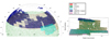 |
Fig. 1. Distribution of the different spectroscopic and lensing samples used in this work. The plot on the left shows the North Galactic Cap (NGC), where most UNIONS galaxies lie. On the right is a portion of the South Galactic Cap (SGC), with the DES Y3 observations in the most southern part. There is no overlap between the UNIONS and DES Y3 catalogues. The apparent variation in shades between the two panels is due to the two projections resulting in different point densities. |
where σSN is the galaxy shape noise and σei represents the variance of the ellipticity component i = 1, 2 estimated by the model fitting procedure.
The PSF was modelled with MCCD2 (Liaudat et al. 2021), a software based on a minimisation scheme analogous to PSFEx, but which includes both a ‘local’ component fitted on a single CCD and a ‘global’ contribution. This coupling allows it to capture effects varying across the entire focal plane.
The objects entering the lensing catalogue are selected with a signal-to-noise ratio of S/N > 10, estimated from the fitted flux divided by the flux error. The UNIONS catalogue reaches an r-magnitude depth of r ≈ 24.7, as shown in Fig. 3. For validation, we compared a correlation function measurement obtained with ShapePipe to one produced with lensfit (shown in Appendix B).
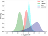 |
Fig. 3. Un-weighted normalised r-band magnitude distributions of the BOSS/eBOSS spectroscopic samples and UNIONS photometric galaxies. We can see that the spectroscopic galaxies from the BOSS/eBOSS surveys fall into the brighter tail of the UNIONS distribution. The galaxies which dominate the lensing signal are comparatively fainter. Note: we could not use our large overlap with LOWZ galaxies as these bright galaxies (r < 20) are mostly absent from our lensing sample due to size cuts. |
2.2. DES Y3 catalogue
For a comparison between UNIONS and DES intrinsic alignment measurements, we reproduced the Dark Energy Survey (DES) measurements close to those presented in Sa23. For this purpose, we used the publicly available DES Y3 Metacalibration shape catalogue. The catalogue is described in Gatti et al. (2021). It contains 100 204 026 galaxies covering 4139 square degrees of sky area. Images were taken in the g, r, i, z, and Y bands and galaxy shapes were fitted on r, i, z band images simultaneously.
The core of the galaxy shear estimation methods is common to DES and UNIONS, which both use the ngmix model fitting software and calibrate the shear response with the Metacalibration scheme. This is critical for our comparison, as it was shown in Georgiou et al. (2019a) and Singh & Mandelbaum (2016) that different shape measurement algorithms can lead to very different intrinsic alignment amplitudes.
To create the shear and redshift galaxy sample, we first matched the BOSS and eBOSS spectroscopic galaxies to the full DES Y3 source galaxies (see Sect. 2.4). We then removed spurious objects by applying cuts based on the size and S/N, as well as the likelihood of being contaminated by binary stars, as described in Gatti et al. (2021). Below we highlight differences between the UNIONS and DES Y3 catalogues and methods which are important in order to compare the measurements from each dataset:
-
DES uses the PIFF (Jarvis et al. 2021) PSF model while the UNIONS catalogue is built with MCCD. PIFF in the DES Y3 setup fits the PSF CCD by CCD, while MCCD captures the entire focal plane at once.
-
UNIONS measures galaxy shapes by fitting the CFHT r band, while DES provides joint fits using the r, i, and z band images.
-
The seeing between the two data sets is very different; UNIONS carried out observations with a median seeing of 0.69″ in r, while DES images have a median seeing of 0.95″, 0.88″, 0.83″ in r, i, and z, respectively (Abbott et al. 2021).
2.3. BOSS/eBOSS catalogues
The BOSS/eBOSS tracer catalogues were selected for galaxy clustering studies. Using these catalogues to measure the intrinsic alignment signal is therefore advantageous, as these galaxies have been selected by phenomenological properties and have a well-characterised galaxy bias. Such homogeneous galaxy samples are not representative of the complete population of a typical weak-lensing galaxy set and the corresponding intrinsic alignment measurements cannot be adopted directly as prior for weak lensing. To measure the intrinsic alignment, we need to model the galaxy bias parameters, over which we perform the marginalisation. Therefore, these parameters need to be well constrained to avoid degeneracies with intrinsic alignment parameters.
The catalogue contains weights for each galaxy described in Reid et al. (2015), Raichoor et al. (2020), which are the product of the following components:
-
wcp, to account for fiber collisions in galaxy pairs;
-
wnoz, to account for model redshift failures;
-
wsys, tot, to remove spurious observationally induced fluctuations of non-cosmological origin;
-
wFKP, to minimise the mean square fluctuations of the density power spectrum, Pδ(k), introduced in Feldman et al. (1994). They are defined as
 with P0 being the value of the power spectrum at k ≈ 0.15 h−1 Mpc and
  the mean galaxy density at a redshift, z.
In the following, we briefly describe the different BOSS/eBOSS samples used in this paper. The redshift distribution of the different samples is shown in Fig. 2.
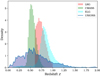 |
Fig. 2. Un-weighted normalised redshift distribution n(z) of the three BOSS/eBOSS galaxy samples. The UNIONS n(z) is approximate and for reference only, as blinding was implemented as a shift in the redshift distribution. The n(z) has been obtained by matching galaxies in the CFHTLenS W3 field and calibrated through deep spectroscopic reference samples. |
2.3.1. CMASS
The eBOSS CMASS sample (Dawson et al. 2013) was selected on stellar masses as a passively evolving galaxy sample. It contains galaxies in the redshift range z ∈ [0.4, 0.8]. The targets were selected using colour cuts for which the philosophy and functioning are presented in Eisenstein et al. (2001). These cuts are i < 19.9, d⊥ > 0.55 and i < 19.86 + 1.6 × (d⊥ − 0.8). The quantity d⊥ = (r − i)−(g − r)/8 quantifies a line in colour space perpendicular to the position of the locus of the desired galaxy population at z > 0.4. For this sample, the combined weight w is
 (2)
(2)
2.3.2. LRG
The eBOSS luminous red galaxy (LRG) DR16 sample (Bautista et al. 2018) was selected with the conditions r − i > 0.98, and r − W1 > 2.0 (r − i), where W1 is the 3.4 μm band from the WISE survey, and the r and i bands are from the SDSS imaging survey. This results in a sample of high-redshift red galaxies with z ∈ [0.6, 1.1].
The total weight for eBOSS LRGs is (Bautista et al. 2020):
 (3)
(3)
2.3.3. ELGs
The eBOSS emission-line galaxy (ELG) sample (Raichoor et al. 2020) is made up of selected ELGs in the range 0.6 < z < 1.1 over an observed sky area of 1170 deg2. The target selection was made via a cut in the g band magnitude, which is sensitive to [OII] emitters, and a box selection in the grz colour space. In the NGC, the g cut is 21.825 < g < 22.9. These galaxies form a younger and bluer sample, which means that no intrinsic alignment is expected in these galaxies and that they have a lower clustering bias. The ELG galaxies follows the weight scheme Eq. (3) adopted in eBOSS for the LRGsample.
2.4. Matching procedure
To obtain a sample with precise redshift information, we matched the publicly available SDSS catalogues described above with the UNIONS shape catalogue introduced in Sect. 2.1. We used the k-D tree implementation in astropy with a tolerance of 1″, which is the maximum distance between galaxy pairs to be considered a match. We obtained the matched sub-sample of our respective catalogues with precise ellipticity and redshift measurements as our shape sample. For the density sample, we use all galaxies of the respective SDSS catalogues. The different properties of the surveys are described in Table 1.
Sample properties used in this work.
3. Correlation and covariance estimations
3.1. Shape-density correlation estimator
To estimate the shape-density correlations of intrinsic galaxy alignment, we use the common projected two-point cross-correlation function wg, + (Mandelbaum et al. 2006). The intrinsic-alignment measurement is similar to galaxy-galaxy lensing, but differs from the latter as the shape tracer can be either at lower or higher redshift compared to the density tracer, at very limited separations along the line of sight.
Following Mandelbaum et al. (2006), we first computed the 3D correlation function using the modified Landy-Szalay estimator:
 (4)
(4)
The variables s, d, and r indicate indices of objects in the shape, density, and random sample, respectively. The estimator is a sum of the tangential shear, γ+, sd, of objects in the shape sample around the density sample, corrected by a contribution of γ+, sr around random points. The normalizing quantity Nr, rs(rt, Π) is the number of pairs between the random position and random shape samples. The pairs are binned in the tangential separations rt and line-of-sight distance Π. The subtraction of the random correlations is introduced to mitigate geometrical effects, for example, the shape correlation with the survey mask.
The bin indicator function Δ of the 2D separation vector x = (x⊥,x∥) is defined as
 (5)
(5)
With this characteristic function, we can separate galaxy pairs into logarithmic perpendicular bins with width Δlog r, and linear radial (line-of-sight) bins with a width, ΔΠ.
Next, we integrate the correlation function Eq. (4) along the line of sight to project out redshift space distortion (RSD) effects stemming from peculiar velocities,
 (6)
(6)
We varied the comoving limit and found a stable value of Πmax = 150 Mpc, which is consistent with previous works (Si15, Sa23). In practice, we use the Treecorr package described in Jarvis (2015) to compute Eq. (4) in slices of ΔΠ = 15 Mpc, and sum up the correlations to obtain wg+.
3.2. Density-density correlation estimator
To estimate the galaxy bias parameters, as motivated in Sect. 4.1, we computed the two-point galaxy correlation function using the Landy-Szalay estimator:
 (7)
(7)
As for the shape-density estimator, the random correlations account for systematic geometrical effects. We integrate along the line of sight to wash out RSD effects:
 (8)
(8)
3.3. Shape-shape correlation estimator
The majority of the intrinsic alignment constraining power is obtained from wg+, as position-shape measurements have a higher S/N than the shape-shape measurements. While wg+ is sensitive to gravitational-intrinsic correlations, as explained in Sect. 4.2.1, the projected shape-shape correlation function w++ is proportional to the intrinsic-intrinsic power spectrum. Previous measurements were presented in Si15, Sa23.
The corresponding estimator is defined as
 (9)
(9)
which is then integrated along the line of sight,
 (10)
(10)
We included this estimator for completeness and for comparison with previous works.
3.4. Computing luminosities
When estimating the intrinsic luminosities, various observational effects that modify the observed galaxy flux have to be corrected. For this we compute k-correction using (Blanton & Roweis 2007) as implemented in the python package k-correct. Furthermore, the e-correction is a quantity that reflects the evolutionary processes of galaxies, such as star formation, aging stellar populations, and mergers of galaxies, which change the galaxy brightness as the universe evolves. We obtained the e-correction from the Ezgal package (Mancone & Gonzalez 2012), for which we assumed the commonly used Bruzual & Charlot (2003) model as the stellar population synthesis model. Lastly, we corrected for the dust extinction with the E-corrections. These values are given by the SDSS catalogue and are based on the Schlegel et al. (1998) maps. To compute the luminosities, we used the DevFlux apertures from the SDSS photometric imaging survey; this allowed us to get an approximation of the SED necessary for the e-correction. The absolute magnitude as a function of the observed SDSS magnitude, r, was computed with the formula
![Mathematical equation: $$ \begin{aligned} M_r = r - 5 \ [{\log }_{10} \left(D_{\rm l}(z)\right) -1 ] - (k+e) + E, \end{aligned} $$](/articles/aa/full_html/2025/07/aa53442-24/aa53442-24-eq15.gif) (11)
(11)
where Dl is the luminosity distance in pc/h. This equation and the correction quantities are well established for red galaxy populations and cannot be generically applied, as they require a good understanding of galaxy evolution. Luminosity mean values for different samples are shown in Table 1. We use this information to split our CMASS galaxies in luminosity sub-samples and compare the luminosity scaling to results obtained from the literature in Sect. 5.3. Our luminosity estimates are in good agreement with those from Sa23, even though we do not expect exact matches as their measurements are based on the DES r band filter, which differs slightly from SDSS. To obtain ⟨L/L0⟩, we used the standard pivot luminosity, L0, defined to match an absolute magnitude of Mr = −22.
4. Modeling intrinsic alignment and galaxy clustering
4.1. Modelling Galaxy clustering
Galaxies are biased tracers of the underlying dark matter field. At the linear level, the relation is simply δg(x) = b1δm(x), which consequently is for the matter power spectrum
 (12)
(12)
where Pδ represents the linear matter power spectrum. We adopted a Eulerian bias model in this work. To go beyond the linear order, we expanded the galaxy overdensity as function of the matter density and tidal field up to second order as
 (13)
(13)
where s is the tidal tensor, introduced in McDonald & Roy (2009), and expressed in Fourier space as
 (14)
(14)
The number of bias parameters that can be constrained by observations depends on the precision of the data, and the angular scales used in the analysis. In this study, we only vary b1 and b2, which is sufficient to obtain a good fit. We fix the values of the remaining bias parameters to
 (15)
(15)
The higher order terms from Eq. (13) can be used to establish an expansion of Pgg (Pandey et al. 2020). We used FASTPT (McEwen et al. 2016) to computes the various perturbation contributions in the expansion.
4.2. Intrinsic alignment models
Ellipticities are commonly decomposed into three components: the shear, γG, the intrinsic ellipticity, γI, and a random contribution, γrand,
 (16)
(16)
The first two components do not account for the entire shape noise. Chisari & Dvorkin (2013) showed that the predicted dispersion of ellipticities using these terms is two orders of magnitude smaller than the observed value. An additional component, γrand, was therefore introduced to quantify unaccounted processes. While not random per se, these processes are not correlated with the large-scale structure; therefore, they form a noise contribution. In the following sections, we present two models to predict γI.
4.2.1. NLA
The non-linear alignment (NLA) model (Bridle & King 2007), derived from the linear alignment model (Hirata & Seljak 2004) quantifies the contribution of intrinsic alignment to the ellipticity. It is based on the study of Catelan et al. (2001), which asserts that the mean intrinsic ellipticities of galaxies forming in a tidal field is related to the Newtonian gravitational potential, ΨP, via the relation
 (17)
(17)
where the derivatives along x and y are taken in the transverse plane. The constant C1 takes the fiducial value of 5 × 10⁻¹⁴ M⊙ h−2 Mpc−3 based on the SuperCOSMOS survey from Brown et al. (2002). This ties the tidal deformations to cosmological quantities as the Newtonian potential can be related to the linear matter overdensities δm via the relation in Fourier space
 (18)
(18)
where  is the rescaled growth factor
  and
and  is the mean density of the Universe.
These relations motivated the expressions of the intrinsic-intrinsic and intrinsic-matter power spectra as
 (19)
(19)
The function F(z) accounts for the pre-factors in the Poisson equation (18),
 (20)
(20)
Here, ρcrit is the critical density of the Universe, and Ωm the matter density parameter, both expressed at z = 0. The AIA parameter is usually left free to account for a varying amplitude of the intrinsic alignment contribution; in this study, we aim to obtain constraints on this parameter. While initially Pδ(k, z) in Eq. (19) was understood as the linear power spectrum, Bridle & King (2007) instead used the non-linear power spectrum to better account for small-scale processes. While not motivated theoretically, this modification provided a better fit to the data and gave rise to the name non-linear alignment model.
4.2.2. TATT
The tidal alignment and tidal torque (TATT) model was introduced as a second-order correction to the NLA model in Blazek et al. (2019), analogous to the inclusion of higher-order biases in galaxy clustering.
An expansion in the linear density field and collection of contributing terms allow us to write the unprojected intrinsic ellipticity tensor as
 (21)
(21)
Summation over repeated indices is implied. The most common parametrisation established in Blazek et al. (2019) defines the first parameter as
 (22)
(22)
which is the parameter already present in the NLA model.
The amplitude of the quadratic contribution of the tidal tensor is parameterised by C2, given by
 (23)
(23)
The term quantifying the correlation between the tidal tensor and the overdensity is
 (24)
(24)
From a theoretical point of view, bTA can be interpreted as the linear galaxy bias b1. In the TATT model, however, it is an additional free parameter quantifying the correlations between the tidal tensor and the galaxy density field. We note that we choose A1, A2, and A1δ to be constant for simplicity, but they can also be specified as a function of redshift. Using these parameters one can establish an expression for PgI and PII. We refer to Blazek et al. (2019) for details.
4.3. Redshift-space distortions
Peculiar velocity effects, known as redshift space distortions (RSDs), induce anisotropies along the line of sight, which have to be accounted for in our theoretical model. RSDs are added at the power-spectrum level following the Kaiser (1987) parametrisation,
![Mathematical equation: $$ \begin{aligned} P_{\rm gg}^s (\boldsymbol{k}, z) = b_1^2 \left[1 + \beta (z) \mu \right]^2 P_{\mathrm{gg}}(k, z), \end{aligned} $$](/articles/aa/full_html/2025/07/aa53442-24/aa53442-24-eq32.gif) (25)
(25)
with μ as the cosine of the angle between k and the line of sight. The superscript s specifies that the power spectrum is defined in redshift space. The function β(z) = f(z)/b1(z) is the ratio of the growth rate f(z) and the linear galaxy bias b1. In the linear regime, only the first three even multipoles are non-vanishing. They are given by Kaiser (1987) as
 (26)
(26)
 (27)
(27)
 (28)
(28)
The configuration-space multipoles can then be estimated by the Hankel transform
 (29)
(29)
where jℓ represent the spherical Bessel functions of order ℓ. The 2D anisotropic two-point correlation function can then be reconstructed as
 (30)
(30)
with  representing the distance between the galaxies. The estimation of wgg is then obtained by integrating ξggs(rt,Π) along the line of sight. We note that wg+ is very mildly affected by RSDs and we did not include these effects here.
4.4. Predicting the projected correlation functions
We modelled the projected correlation functions measured in Eqs. (6), (8) and (10) via a Limber projection, and using a Hankel transform:
![Mathematical equation: $$ \begin{aligned} { w}_{\rm gg}\left(r_{\rm t}\right) =&\int \mathrm{d} z \, \mathcal{W} ^{\mathrm{dd} }(z) \int \frac{\mathrm{d} k_{\perp } k_{\perp }}{2 \pi } \mathrm{J}_0\left(k_{\perp } r_{\mathrm{t} }\right) P_{\rm gg}\left(k_{\perp }, z\right); \nonumber \\ { w}_{\rm g+}\left(r_{\mathrm{t} }\right) =&-\int \mathrm{d} z \mathcal{W} ^{\mathrm{ds} }(z) \int \frac{\mathrm{d} k_{\perp } k_{\perp }}{2 \pi } \mathrm{J}_2\left(k_{\perp } r_{\mathrm{t} }\right) P_{\rm gI}\left(k_{\perp }, z\right); \nonumber \\ { w}_{++}\left(r_{\mathrm{t} }\right) =&\int \mathrm{d} z \mathcal{W} ^{\mathrm{ss} }(z) \nonumber \\&\times \int \frac{\mathrm{d} k_{\perp } k_{\perp }}{4 \pi } \left\{ \left[\mathrm{J}_0\left(k_{\perp } r_{\mathrm{t} }\right) + \mathrm{J}_4\left(k_{\perp } r_{\mathrm{t} }\right)\right] P_{\mathrm{II,EE} }\left(k_{\perp }, z\right) \right. \nonumber \\&\left. + \left[\mathrm{J}_0\left(k_{\perp } r_{\mathrm{t} }\right) - \mathrm{J}_4\left(k_{\perp } r_{\mathrm{t} }\right)\right] P_{\mathrm{II,BB} } \right\} . \end{aligned} $$](/articles/aa/full_html/2025/07/aa53442-24/aa53442-24-eq39.gif) (31)
(31)
The function Jν is the first-kind Bessel function of an order, ν, and 𝒲ij is the projection kernel (Mandelbaum et al. 2011) given by:
![Mathematical equation: $$ \begin{aligned} \mathcal{W} ^{ij}(z) = \frac{n^i(z) n^j(z)}{\chi ^2(z)\,\mathrm{d}\chi /\mathrm{d}z} \times \left[\int \mathrm{d} z\prime \frac{n^i(z\prime ) n^j(z\prime )}{\chi ^2(z\prime ) \mathrm{d}\chi /\mathrm{d}z\prime }\right]^{-1}. \end{aligned} $$](/articles/aa/full_html/2025/07/aa53442-24/aa53442-24-eq40.gif) (32)
(32)
χ(z) is the comoving distance at distance z, and ni(z) is the redshift distribution of the shape (i = s) or density (i = d) sample.
4.5. Modelling the lensing contamination
By construction, the estimator wg+ defined in Eq. (5) is able to pick out intrinsic-alignment correlations at high S/N values. It is, however, also sensitive to a number of other parameters and effects. Some of these effects include a marginalisation over cosmological parameters, baryonic feedback, weak gravitational lensing magnification and shape correlations. In this section, we focus on the latter source of contamination.
To account for the lensing contribution in our measurement, we follow the method of Joachimi et al. (2011), Tonegawa & Okumura (2022). The galaxy-galaxy lensing contribution is given by the angular power spectrum (Joachimi et al. 2011)
 (33)
(33)
This requires knowledge of the galaxy bias. The density tracer px(χ, χ1) and the lensing kernel qε(χ′,χ(z2)) are given in full generality for a photometric survey. With spectroscopic surveys, the conditional density tracer px(χ|χ1) simplifies to the n(χ1) as spectroscopic redshift estimates can be considered exact at the precision we work at. This implies that the lensing kernel is expressed as:
 (34)
(34)
It can be further simplified by the insertion of a Dirac delta as px(χ′|χ1):
 (35)
(35)
This allows to rewrite Eq. (33) in the simpler form:
 (36)
(36)
Now we do not express our correlation function in terms of χ1, χ2, but we instead use the coordinate system, rt, Π, in physical space. To transform the coordinates, we need to start by defining new coordinates which relate the two systems:
 (37)
(37)
As we need the correlation functions for a variety of zm, Π, rt we built a grid of ξ(θ, z1, z2) in the z1, z2 space. We therefore have a grid of correlation functions that we can then use to evaluate the integrated correlation function:
 (38)
(38)
The kernel here is described in Eq. (32). The weak-lensing contribution has a scale dependence which is analogous to the intrinsic alignment signal on the scales of interest and contributes 1% for CMASS-UNIONS, 3% for LRG-UNIONS, and 6% for ELG-UNIONS. This is consistent with the findings in Sa23 when we make adjustments for the relative signal amplitudes.
Regarding the other sources of contamination to the integrated correlation function listed above are sub-dominant on the scales of interest, and we choose, therefore, not to model them here. The marginalisation over cosmological parameters has been studied and we refer to Johnston et al. (2019) for more details.
4.6. Covariance matrix
4.6.1. Analytical covariance matrix
To estimate the covariance matrix for our different estimators, we use an analytical model, which was first described in Chisari & Dvorkin (2013), and used in Samuroff et al. (2021) and Sa23. To compute the covariance matrix we follow the procedure laid out in Samuroff et al. (2021). We compute the full covariance matrix of the joint vector containing the integrated correlation functions wg+, wgg, w++. Each block of the analytical covariance matrix can be decomposed into three types of contributions: a Gaussian part that accounts for cosmic variance, a shot noise part, and a mixed term.
The full general equation for the covariance matrix between two integrated correlation function estimates wαβ and wγε for α, β, γ, ε ∈ [g, +] at angular scales rt, i and rt, j is given by
![Mathematical equation: $$ \begin{aligned}&\mathrm{Cov}\left[{ w}_{\alpha \beta }\left(r_{\mathrm{t} , i}\right) { w}_{\gamma \varepsilon }\left(r_{\mathrm{t} , j}\right)\right] = \frac{1}{\mathcal{A} \left(z_{\rm eff}\right)} \int _{0}^{\infty } \frac{k\,\mathrm{d}k}{2\pi } \bar{\Theta }_{\alpha \beta } \left(k r_{\mathrm{t} , i}\right) \bar{\Theta }_{\gamma \varepsilon } \left(k r_{\mathrm{t} , j}\right)\nonumber \\&\times \left[(P_{\alpha \gamma }(k) + \delta _{\alpha \gamma } N^{\alpha }) \times (P_{\beta \varepsilon }(k) + \delta _{\beta \varepsilon } N^{\beta })\right.\nonumber \\&\left.\qquad \qquad \qquad + (P_{\alpha \varepsilon }(k) + \delta _{\alpha \varepsilon } N^{\alpha }) \times (P_{\beta \gamma }(k) + \delta _{\beta \gamma } N^{\beta })\right]. \end{aligned} $$](/articles/aa/full_html/2025/07/aa53442-24/aa53442-24-eq47.gif) (39)
(39)
The pre-factor is the inverse of 𝒜(zeff), the comoving area at redshift zeff. To obtain this effective redshift, we take the average of the sample redshift distribution n(z), weighted by the square of the number of galaxy pairs Ngal2(z). This is motivated by the fact that the integrated correlation function wαβ is sensitive to the number of galaxy pairs. When the shape and density samples differ for wg+, we use the effective area of the smaller sample, as this is where pairs are formed. The effective redshift approximation is accurate for our samples but might need to be refined for more complex redshift distributions. We will improve upon this approximation in future work.
The  functions are bin-averaged Bessel functions,
 (40)
(40)
with Ai the area of bin i, Θgg = J0, Θg+ = J2 and Θ++ = J0 + J4.
The two different shot-noise terms are  corresponding to Poisson noise from discrete galaxy positions, and
  from intrinsic galaxy shapes3. We use σε as the single-component shape noise term defined in Gatti et al. (2021) as
![Mathematical equation: $$ \begin{aligned} \sigma _e^2 = \frac{1}{2} \left[\frac{\sum _i \left({ w}_i e_{i, 1}\right)^2}{\left(\sum _i { w}_i\right)^2} + \frac{\sum _i \left({ w}_i e_{i,2}\right)^2}{\left(\sum _i { w}_i\right)^2}\right] \left[\frac{\left(\sum _i { w}_i\right)^2}{\sum _i { w}_i^2}\right]. \end{aligned} $$](/articles/aa/full_html/2025/07/aa53442-24/aa53442-24-eq52.gif) (41)
(41)
The estimator with the highest S/N carrying the bulk of information on intrinsic-alignment parameters is the shape-density integrated correlation function wg+ defined in Eq. (31). We explicitly write out the covariance Eq. (39) for the special case of (αβ) = (γε) = (g + ) as
![Mathematical equation: $$ \begin{aligned} \mathrm{Cov}&\left[{ w}_{\rm g+}\left(r_{\mathrm{t} , i}\right) { w}_{\rm g+}\left(r_{\mathrm{t} , j}\right)\right] = \frac{1}{\mathcal{A} \left(z_{\rm eff}\right)} \int _{0}^{\infty } \frac{k\,\mathrm{d}k}{2\pi } \bar{\Theta }_{\alpha \beta }\left(k r_{\mathrm{t} , i}\right) \bar{\Theta }_{\gamma \varepsilon } \left(k r_{\mathrm{t} , j}\right)\nonumber \\&\times \left[\left(P_{\rm gg}(k) + \frac{1}{\bar{n}_{\mathrm{density} }(z_{\rm eff})}\right) \times \left(P_{\rm II}(k) + \frac{\sigma _\varepsilon ^2}{\bar{n}_{\mathrm{shape} }(z_{\rm eff})}\right) + P^2_{\rm gI}(k)\right]. \end{aligned} $$](/articles/aa/full_html/2025/07/aa53442-24/aa53442-24-eq53.gif) (42)
(42)
The mixed power spectrum PgI2(k) does not have a shot-noise contribution as it corresponds to a cross-correlation, resulting in the corresponding Kroenecker deltas in Eq. (39) to vanish.
We plot the diagonal of this covariance in Fig. 4. On small scales, the covariance matrix is shot-noise dominated. On larger scales, the mixed term of the clustering power spectrum and galaxy shape noise becomes the leading term. We note that this mixed term is missing from the covariance matrix of Sa23 (their Eqs. 26 and 27). Since this term is dominant for rt ⪆ 20 Mpc, this omission resulted in a bias of their results, and an underestimation of the error bars published in Sa23. We confirmed this finding by applying our analytical covariance matrix without this mixed term to DES Y3 data, leading to the same biases as in Sa23. We note that this term was still present in the earlier publication Samuroff et al. (2021). In Sect. 5, we present a re-analysis of the DES Y3 and BOSS correlations and show the corrected intrinsic-alignment constraints.
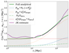 |
Fig. 4. Square root of the diagonal of the analytical covariance matrix of wg+ for the CMASS-UNIONS sample (green solid line). The individual contributions are cosmic variance (dashed; the PggPII term is identical to the PgI contribution); mixed clustering – ellipticity shot noise (dotted); mixed intrinsic – density shot noise (long dash-dotted); and pure shot noise (short dash-dotted). See Eq. (42) and text for details. For comparison, we plot the jackknife variance (purple solid line), which is in excellent agreement with the analytical covariance over the relevant scales. |
4.6.2. Jackknife covariance matrix
To validate our analytical covariance matrix, we compared it to a data resampling covariance using the jackknife method (Si15, Johnston et al. 2019; Fortuna et al. 2021b; Joachimi et al. 2011). We split the observed area into ns patches using the K-means algorithm implemented in Treecorr. A number of ns realisations were built by removing one patch from the data set at a time. The correlation function was computed on the remaining data. The idea is that the patches contain the largest scales probed by the correlation function. By removing a patch, we can estimate the variation in the data without any external analytical formulation or simulation. The jackknife estimation of the covariance matrix is given by:
 (43)
(43)
with  as the k-th correlation function computed from the ns jackknife samples. The ij indices are the bins in rt between which we want to compute the covariance. The average
  is taken over the ns jackknife estimations.
Figure 4 shows the excellent agreement between the analytical and jackknife covariance over the angular scales of interest. Since the jackknife covariance is noisy, in particular on the off-diagonal elements (Samuroff et al. 2021), we used the analytical covariance for the parameter inference.
4.7. Scale cuts
As described in Sect. 2.3, the eBOSS samples were originally selected for galaxy clustering on large scales, with the explicit goal of measuring the baryonic acoustic oscillation scale around 100 h−1 Mpc. The sample has therefore not been optimised for small-scale correlations, where the intrinsic alignment becomes most relevant. To include smaller scales would require a more densely sampled survey such as GAMA or DESI.
Furthermore, we did not include small scales in our analysis as baryonic feedback and non-linearities can become dominant on these scales. To be consistent with previous works, we introduced a small-scale cut at 9 Mpc (Joachimi et al. 2011, Si15, Sa23). We also excluded points above 100 Mpc from the fit. This was motivated by the projection effects described in Singh & Mandelbaum (2016): The integration over Π along the line of sight causes a suppression for large Π, as galaxy shapes pointing towards the density tracer at large line-of-sight separation will appear smaller along the radial axis when projected on the 2D observer plane. While this projection effect exists at all transverse separations rt, it is sub-dominant where the amplitude of wg+ is large. The sensitivity of wg+ to PgI in the [rT, Π] plane is quantified in Joachimi et al. (2011). To mitigate these projections effect, the 3D Yamamoto estimator (Kurita et al. 2021) or the real-space 3D correlator (Singh et al. 2024) can be used, which circumvent the issue by using the full 3D information.
For consistency with previous works (Sa23), we take 21 log-spaced bins in the range rt ∈ [0.1, 350] Mpc to compute our projected correlation functions. For the cosmological parameters we assumed h = 0.69, nS = 0.97, AS = 2.15 × 10⁻⁹, and Ωm = 0.3. We used the emcee package to fit our models. All correlation functions are computed with the TreeCorr package (Jarvis 2015).
5. Results
5.1. Integrated correlation functions
We show in Fig. 5 the measurement of wg+ and w++ for the different UNIONS-BOSS/eBOSS samples as described in Sect. 2. We observe strong intrinsic alignment in our two red galaxy samples, CMASS and LRG, consistent with what has been shown in the literature. In grey, we shade the areas excluded from the fit, as motivated in Sect. 4.7. For CMASS-UNIONS, our measured wg+ is well fitted by the NLA model down to scales of rt ≈ 5 Mpc. Below this scale, the CMASS galaxies are sparsely sampled, and we therefore do not see the appearance of a one-halo term. Overall we remain on linear scales where the NLA model performs well. The w++ plot shows an apparent positive correlation, which seems under-fitted by the NLA model. The reduced χ2 summarised in Table 2 indicates that the fit is good, but the null hypothesis is also not excluded for this data vector. Our fit of  represents one of the most significant detections in the literature.
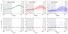 |
Fig. 5. Measurements of wg+ (upper panels) and w++ (lower row) for the UNIONS-CMASS (left), UNIONS-LRG (middle), and UNIONS-ELG (right column) samples. The solid lines show the best-fit NLA model, where the shaded areas indicate the 1σ uncertainty associated with the fit. The grey areas are excluded from the fit as explained in Sect. 4.7. |
In the LRG sample, the picture is similar, although the measurement is slightly more scattered. The fit follows the data points well down to scales of rT ≈ 8 Mpc. The large error bars are due to the scarce density of the LRG galaxies, which in turn are responsible for the large uncertainty on the AIA fit, even though the 80 000 galaxies form a consequential sample for this type of measurement. The w++ correlation function is noisy and has negative points. Its error bars are shot-noise dominated and we do not give any strong interpretation of w++ as the measurement is compatible both with the NLA model and with the null hypothesis. The total fit gives  , a value we compare to other measurements in Sect. 5.4.
For the ELG sample, we expected no intrinsic alignment signal as this is a sample mainly composed of blue galaxies. These have repeatedly shown to exhibit intrinsic alignment amplitudes consistent with zero. While we have measured a relatively high value of AIA, the error bars are still compatible with AIA = 0 at the 1.1σ level. The w++ vector also appears to exhibit a strong correlation on larger scales, but here again, the points are correlated and the data vector is compatible with the null hypothesis.
All results are summarised in Table 2. The global reduced χ2 indicates that our overall fit is good. We note that while we report the individual reduced χ2 for each data vector separately, they are for reference only as the fit is performed jointly on all 3 data vectors, and the covariance between them is not negligible. We considered 5 degrees of freedom for w++ and wg+ (6−1), 6 for wgg (8−2) and 17 for the total fit (20−3).
Mean and standard deviations of the posterior distributions of the three parameters and the reduced χ2 values associated with the diagonal blocks of the covariance matrix.
5.2. Model comparison
With our high S/N measurement, we test the TATT model (Blazek et al. 2019) to see if the additional degrees of freedom can help in modelling the wg+ signal. The TATT model is a higher-order expansion, as explained in Sect. 4.2.2. We therefore fit wg+ and w++ down to 4 Mpc. The constraints on the second-order TATT parameters from CMASS-UNIONS can be seen in Fig. 7. From Fig. 6, the NLA and TATT best-fit models are in very good agreement, within 1σ down to small scales. It appears that the scales outside the fitted range are better captured by the NLA model. Considering the reduced χ2 we get,
 (44)
(44)
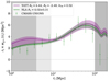 |
Fig. 6. Best-fit lines and 1σ contours for the NLA and TATT, respectively. The TATT model is fit down to 4 Mpc but both models appear very consistent. The 1σ TATT contours are obtained by drawing 500 models from the posterior and calculating the 68% confidence interval at eat rt. |
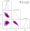 |
Fig. 7. Posterior contours of the NLA and TATT model fitted to the CMASS-UNIONS sample. We see no deviation from the NLA case as A2 and bTA appear consistent with 0. |
These reduced χ2 have been obtained for the full data vectors meaning, 8 + 6 + 6 − 3 degrees of freedom for NLA and 8 + 8 + 8 − 5 degrees of freedom for TATT. To compare them, we can use the Bayesian information criterion (BIC) defined as
 (45)
(45)
where k is the number of parameters and Np is the number of fitted points. The BIC is a commonly employed metric which balances goodness of fit and model complexity by penalizing an excessive number of parameters, which would indicate overfitting. We respectively obtain:
 (46)
(46)
From ΔBIC(TATT − NLA) = 7.9 we conclude that the additional TATT degrees of freedom are not needed here. We can nevertheless make a few observations, as follows. First, the A1 and A2 parameters are strongly degenerate. This is expected as A1 is the proportionality factor for sij, and A2 for sij2, displaying similar behaviour for small values of the tidal tensor. To decorrelate the two parameters, the largest possible variations of the tidal field must be probed so that the linearisation breaks down and the quadratic regime can be distinguished from the linear regime. It is not obvious if this will happen on scales relevant for weak lensing, since we are in the perturbation-theory domain where variations are small.
Furthermore, we observe a degeneracy between bTA and A2. As bTA is multiplied with the overdensity δmsij, a similar argumentation holds for these two parameters as for the (A1, A2) pair. From theoretical arguments bTA can be expected to be comparable to b1 as it correlates the tidal tensor with the overdensity field, traced here by galaxies. The fact that we constrain bTA to values compatible with zero, far away from b1 ≈ 2, can be an indication that the linear assumptions allowing us to take the product of the linearised density field with the tidal tensor can not be naively applied here.
Finally, we see no correlation between bTA and A1. This can be interpreted by the model picking up on the density field and decorrelating it from the tidal tensor. As both parameters are multiplied with each other to form the parameter Ad, the fact that raising one is not simply equivalent to lowering the other indicates that the measurement effectively decorrelates matter variations from tidal-field modifications. Upcoming measurements will allow us to go down to smaller scales and properly understand the behaviour of these parameters for different samples.
5.3. Luminosity dependence
We measured the luminosity scaling of our intrinsic-alignment measurements of red galaxies and compared the results to previous studies. As described in Sect. 3.4, multiple observations have shown a correlation between luminosity and intrinsic alignment. Such a correlation is motivated by recent findings in Fortuna et al. (2025), who showed that luminosity scales with halo mass. A similar correlation was already hinted at in Xu et al. (2023b). This explains why luminosity is a good predictor of intrinsic alignment, as halo masses determine the amplitude of the tidal field. In Fig. 8 we plot our UNIONS measurements for the CMASS sample split into three equi-populated bins with limits log(L/L0)∈[−0.8; −0.14; 0.12; 0.6]. The intrinsic-alignment amplitude shows a clear increase with luminosity. Results are shown in Table 3.
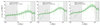 |
Fig. 8. Integrated correlation function, wg+, as measured on the CMASS-UNIONS sample split in 3 bins of luminosity, showing increasing luminosity from left to right panels. One can see a clear increase in the amplitude of the signal. |
Luminosity and intrinsic alignment amplitudes for the CMASS samples split into luminosity bins.
Fig. 9 shows the NLA amplitude AIA from our UNIONS and DES measurements with the CMASS and LRG samples, together with a collection of data points from the literature. Our samples are in agreement with measurements from Joachimi et al. (2011), Si15, Johnston et al. (2019), Fortuna et al. (2021b). The CMASS-UNIONS points are slightly higher than the CMASS-DES points, but both seem to scale in the same way with luminosity. On the contrary, the LRG-UNIONS point is lower than the LRG-DES point. We will come back to this discrepancy in Sect. 5.4.
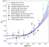 |
Fig. 9. Intrinsic alignment amplitude as a function of luminosity as measured by different surveys. The fitted function is α⟨L/L0⟩β. We can see very similar scaling with luminosity when comparing our CMASS-DES and CMASS-UNIONS measurements. |
To quantify the luminosity-dependence and evolution of the intrinsic-alignment amplitude, we fitted all data points from Fig. 9, assuming their independence. Various functional forms have been tested; Joachimi et al. (2011) introduced a scaling relation of
 (47)
(47)
Motivated by recent works which disfavour any strong z-dependency (Si15; Johnston et al. 2019; Sa23), we fixed η = 0. In addition to this single-power-law model, a broken power law was introduced in Fortuna et al. (2021b) to better account for the flattening of the AIA − log L relation at low luminosities.
We test the single and double power law models, defined as:
 (48)
(48)
Figure 9 demonstrates that both models provide decent fits to the data. The reduced χ2 for the single and double power-law are χ2 = 2.42 with 28 degrees of freedom (30−2) and χ2 = 2.19 with 26 degrees of freedom (30−4), respectively. These high values of reduced χ2 indicate that both models perform rather poorly which is expected given the scatter in Fig. 9. We can compute the BIC and thus obtain:
 (49)
(49)
The difference ΔBIC(SPL − DPL) = 4.0 indicates that the double power law is slightly favoured, a result consistent with the recent literature.
While converging on the AIA(L) relationship is important, we want to highlight the complexity that Fig. 9 is omitting by using a single predictive parameter. While the redshift dependence has been found to be sufficiently well captured by the naïve NLA model, many observational properties strongly affect the intrinsic alignment amplitude, as explained in the introduction. One can therefore not apply this intrinsic alignment-luminosity relationship to derive priors for a different survey without taking the risk of biasing the measurements. Including additional effects which explain the scatter in Fig. 9 will be the subject of a future work. Figure 3 shows that these spectroscopically selected galaxies have apparent magnitudes which fall inside our UNIONS source sample, although they are within the bright tail of the distribution. To establish a reliable prior, it is essential to map the intrinsic alignment amplitudes across redshift, luminosity, and colour space, for the entire weak-lensing source sample, with sufficient accuracy. Achieving better coverage of this three-dimensional parameter space requires either complete spectroscopic samples which include fainter objects, or deep narrow-band fields that provide reliable photometric redshifts for all galaxies. This study examines only a small subset of this parameter space. However, the agreement between different surveys, as discussed in Sect. 5.4, is a necessary step for further progress.
5.4. Comparing UNIONS to other lensing samples
One of the main motivations of this work is a comparison of the measured intrinsic alignment quantities between UNIONS and DES Y3. The interest lies in the understanding of the universal nature of intrinsic alignment. As stated in the introduction, observational effects can influence this kind of measurement. Important effects discussed in the literature include the galaxy shape measurement method or the colour of the sampled galaxies. Here, we have a unique opportunity to study a homogeneous set of galaxies selected by the SDSS imaging survey, with two distinct shape measurement catalogues. While a number of similarities can be noted in the ShapePipe and DES Y3 pipelines, a few important differences between the two datasets exist, as explained in Sect. 2. A good agreement between the UNIONS and DES Y3 constraints would, therefore, indicate a certain control on the effects affecting intrinsic alignment measurements. This is crucial if one wants to use existing measurements as a prior for future surveys such as Rubin/LSST and Euclid. Tight priors improve the statistical power to constrain cosmological parameters but will induce biases if inaccurate.
To test the compatibility of different shape measurement samples, we can compare our measurements to a third dataset for the CMASS-type galaxies (Kurita & Takada 2023). This dataset has the advantage of covering the entire CMASS sample and, therefore, overlaps with both UNIONS and DES. That study was performed with a newly developed, more accurate, 3D correlation function estimator (Kurita et al. 2021), which decreases the error bars on the estimated parameters. Their measurement relies on the shape catalogue described in Reyes et al. (2012), Mandelbaum et al. (2013), which is based on the ‘re-Gaussianisation’ method described in Hirata & Seljak (2003). This method computes moments of the shape and corrects for a non-Gaussian PSF. We note that we make use of this shape catalogue for LOWZ shapes with which we validate our pipeline in Appendix A.
In Fig. 10, we show the overlap between the different posteriors. For the CMASS density tracer, the UNIONS and DES Y3 posteriors agree at 1.20σ. The samples do not differ in image selections but they differ slightly in redshift. The DES Y3 sample was chosen in the range z ∈ [0.4, 0.6], the UNIONS sample covers the range z ∈ [0.4, 0.7], and the Kurita sample is in the range z ∈ [0.5, 0.7]. From previous studies on redshift dependence, we do not anticipate these discrepancies to result in significant variations. Although Fig. 10 might suggest a coherent north-south difference in intrinsic alignment, we do not consider this significant, given the inversion of the UNIONS and DES amplitudes in the LRG plot. Nonetheless, we report the differing mean galactic extinctions in Table 1, as this is the only spatially correlated property we could identify that might influence shape measurements.
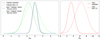 |
Fig. 10. 1D marginal posterior of the NLA intrinsic-alignment amplitude AIA of the same SDSS density tracer. Left panel: UNIONS, DES Y3 (both our measurements), and the results from Kurita & Takada (2023) in the North (NGC) and South Galactic Cap (SGC) using CMASS as density tracer. Right panel: Our measured UNIONS and DES Y3 results with the LRG sample. |
For the LRG sample, we find an agreement between the DES and UNIONS measurements at the 1.51σ level. We conclude that as long as the error bars are properly taken into account the measurements are in sufficiently good agreement to form a prior for stage IV surveys.
5.5. Systematic diagnostics
In Fig. 11, we show the cross-modes, wg×, computed from our samples. These are expected to be compatible with zero in the absence of systematic contributions (Joachimi et al. 2011), analogously to lensing B-modes in cosmic shear. In Table 4 we show the deviation from zero of the cross-mode wg×, and compare it to the one of the intrinsic-alignment mode wg+. We convert the reduced χ2 into a Gaussian σ estimate for easier interpretation. The cross-mode wg× is compatible with zero at 1σ for all samples, which strengthens the confidence in our results. In contrast, the deviations from zero for wg+ testify of our high S/N measurement. For the ELG sample, both wg+ and wg× have remained consistent with zero at the 1σ level.
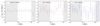 |
Fig. 11. Measurements of wg× for the CMASS-UNIONS, LRG-UNIONS and ELG-UNIONS samples. Deviations from 0 are characterised in Table 4 and are all compatible at the 1σ level. |
Table testing the compatibility with the null hypothesis of the different samples.
5.6. Quantifying PSF errors
The effects of PSF mispecifications on cosmic shear have been studied in detail (Heymans et al. 2012; Jarvis et al. 2021; Giblin et al. 2021). Even small PSF residuals can produce biases in cosmological analyses and mimic the correlations induced by weak gravitational lensing. Quantities such as PSF leakage (Jarvis et al. 2016), ρ-statistics (Rowe 2010), and τ-statistics (Gatti et al. 2021; Guerrini et al. 2024) have been introduced to measure and marginalise over the biases. For direct measurements of intrinsic alignments, the impact of PSF errors has been less studied, as their effect is comparatively weaker. Singh & Mandelbaum (2016) computed the additive bias from PSF mis-modelling using the quantity
 (50)
(50)
This allows us to quantify a systematic contribution to the shape-shape correlation function ξ++ given by
 (51)
(51)
A shape measurement method that does not correct for the PSF, such as the isophotal method used in Singh & Mandelbaum (2016), can display a large amplitude of APSF.
Given the progress in imaging and shape measurement in recent years and the increasingly stringent requirements on additive biases, we calculate this quantity. As shown in Fig. 12, we measure values of below 2% for our red galaxies, which is sufficiently low to be ignored within our analysis. Interestingly, it varies between samples, which is the effect of a varying leakage across size and S/N, see also Li et al. (2023). In contrast to red galaxies, we find a 4% additive bias for the ELG sample; such a bias can be calibrated via subtraction as in Li et al. (2023). We will address this in future work, as the current error bars on the ELG-UNIONS sample are large due to the limited number of galaxies available for this study.
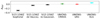 |
Fig. 12. Amplitude expressed by Eq. (50) of the additive bias contamination of the shape-shape correlation function. From left to right, we show our measurements using the Si15 data corresponding to the isophotal, de Vaucouleurs, and re-Gaussianisation shape catalogues, followed by UNIONS-CMASS, UNIONS-LRG, and UNIONS-ELG. |
The measurement of APSF informs us about additive leakage to the shape-shape correlation. Multiplicative and additive biases due to PSF contamination for shape-density correlations have been recently quantified in Zhang et al. (2024) (hereafter Z24). Additive biases are not expected to contribute significantly, since the UNIONS PSF is not expected to show a dependence on the positions of SDSS galaxies. The so-called λ-statistics developed in Z24 allow us to quantify the presence or absence of such biases. A multiplicative bias induced by the PSF can act as an additional calibration factor. In Z24 λ-statistics were introduced for galaxy-galaxy lensing. Here, we adapt their work for the intrinsic-alignment correlation function, wg+.
We started with the PSF error propagation model from Paulin-Henriksson et al. (2008),
 (52)
(52)
In this model, the multiplicative bias term m and additive bias term c do not capture PSF information, which differs from the standard generic parametrisation where m and c represent jointly all systematic contributions. The PSF leakage term αεpsf captures a residual shape contribution from leakage of the PSF, typically attributed to an inaccurate PSF correction during the shape measurement process. The δε term, on the other hand, captures residuals in the PSF measurement at the galaxy position and is due to errors in PSF measurement, modelling, and interpolation and can be understood as a PSF additive bias.
To estimate the PSF error at the galaxy position Paulin-Henriksson et al. (2008) derived a formula using Gaussian error propagation of:
 (53)
(53)
The residuals on the ellipticity, δεpsf, and size, δTpsf, were obtained from a set of reserve stars, which are not used in the PSF modelling process. As we did not have access to this information at each position, we treated these residuals statistically as a constant pre-factor.
With wg+ we can correlate the intrinsic ellipticity with the position of a close-by galaxy (i.e.  ) via the estimator
 (54)
(54)
We use ξ+obs to denote the observed correlation function and ξ+theo as the underlying correlation of the intrinsic shape we are trying to quantify. We can define the change in correlation induced by a PSF mis-specification as
 (55)
(55)
By plugging Eq. (52) into Eq. (54) we can write:
 (56)
(56)
The  contribution vanishes as intrinsic ellipticities do not correlate with random foreground positions. This allows us to define the λ-statistics,
 (57)
(57)
Since we do not expect the UNIONS PSF to be correlated with SDSS positions as stated above, the density tracer n can here be considered as random positions. The λ-statistics then indicate additive errors due to random PSF errors, and potential PSF correlations with the mask or the survey footprint.
The computation of λ1, λ2, λ3, and α are detailed in Z24. With that, we rewrite the PSF contamination with respect to ξ+ as
 (58)
(58)
We can remove the dependence on the theoretical prediction ξ+theo by combining Eqs. (55) and (58) to write the bias of the measured quantity,
 (59)
(59)
To obtain the contamination with respect to wg+, we considered ∫ΠminΠmaxδξ+dΠ. We plot δwg+/wg+ for the CMASS, LRG, and ELG samples in Fig. 13. The PSF contamination remains under 2% on the scales of interest. This indicates that PSF errors are subdominant compared to our statistical power. In the future, when direct intrinsic alignment measurements reach precisions of a few percent, a significant measurement of PSF-tracer correlations can be used to account and calibrate PSF biases.
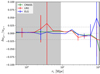 |
Fig. 13. Relative contribution to the wg+ signal of PSF induced correlations. We see that on the scales of interest the contribution is below 2% which we judge satisfactory for current precision. The error bars blow up when wg+ is close to 0. |
6. Conclusion
In this paper, we made use of the UNIONS shape catalogue and the broad overlap with BOSS/eBOSS spectroscopy to carry out a direct measurement of the intrinsic alignment of galaxies. We obtain very significant measurements using 201 639 CMASS, 78 134 LRG, and 14 762 ELG galaxies. Our results are consistent with previous studies showing a strong intrinsic alignment for red galaxies and an alignment compatible with zero for ELGs. These results demonstrate that the UNIONS observations, thanks to their excellent image quality, form a competitive dataset with which we are able to measure the intrinsic alignment in the northern sky. In particular, we highlight the following points:
-
We obtained detections of intrinsic alignment at 13σ with CMASS, at 3σ with LRG and at 1σ with ELG. The latter result is compatible with the null hypothesis. The NLA model was able to produce a compelling fit for these measurements in the range of rt ∈ [9, 100] Mpc.
-
We tested whether the highest S/N measurement (CMASS-UNIONS) would allow for a detection of the higher-order terms of the TATT. To that end, we fit transverse scales down to 4 Mpc. We found no preference for non-zero values of these parameters. However, in the data, the tidal field contribution, A1, de-correlated from the density × tidal field contribution, bTA. The BIC result seems to indicate a preference for the linear NLA model over TATT.
-
Our measured NLA intrinsic-alignment amplitude scales with the luminosity, as also observed in the literature. A double power law seems to provide a reasonable fit, although the reduced χ2 is large due to the high scatter.
-
By adapting a novel framework from Z24, we estimated the bias contributions of the PSF leakage to the intrinsic alignment measurement, which is below 2%.
-
The cross-component wg× was measured to be consistent with zero at 1σ for all samples, indicating an absence of obvious systematic contributions.
-
We re-analysed the DES Y3 data, and find intrinsic-alignment amplitude in agreement with UNIONS, at 1.2σ for CMASS and 1.5σ for LRGs. We found further agreement with other measurements obtained in Kurita & Takada (2023) for CMASS galaxies. We conclude that all of these measurements are compatible with each other and, therefore, they can serve as the basis for an informative prior for stage-IV surveys, as long as the uncertainties are properly accounted for.
This work demonstrates that the UNIONS sample is mature and ready for competitive science cases. In the near future, we aim to use the upcoming spectroscopic data in the northern hemisphere to probe the intrinsic alignment on smaller scales and across a wider ranger of colours and luminosities. The goal is to improve our understanding at the dawn of stage-IV weak lensing surveys.
Sa23 indicates 1/Npairs as their shot noise, which we found to be a negligible contribution.
Acknowledgments
We thank Benjamin Joachimi and Elisa Chisari for informing discussions. FHP acknowledges support from the Centre National d’Études Spatiales (CNES). We are honored and grateful for the opportunity of observing the Universe from Maunakea and Haleakala, which both have cultural, historical and natural significance in Hawaii. This work is based on data obtained as part of the Canada-France Imaging Survey, a CFHT large program of the National Research Council of Canada and the French Centre National de la Recherche Scientifique. Based on observations obtained with MegaPrime/MegaCam, a joint project of CFHT and CEA Saclay, at the Canada-France-Hawaii Telescope (CFHT) which is operated by the National Research Council (NRC) of Canada, the Institut National des Science de l’Univers (INSU) of the Centre National de la Recherche Scientifique (CNRS) of France, and the University of Hawaii. This research used the facilities of the Canadian Astronomy Data Centre operated by the National Research Council of Canada with the support of the Canadian Space Agency. This research is based in part on data collected at Subaru Telescope, which is operated by the National Astronomical Observatory of Japan. Pan-STARRS is a project of the Institute for Astronomy of the University of Hawaii, and is supported by the NASA SSO Near Earth Observation Program under grants 80NSSC18K0971, NNX14AM74G, NNX12AR65G, NNX13AQ47G, NNX08AR22G, 80NSSC21K1572 and by the State of Hawaii. LB is supported by the PRIN 2022 project EMC2 – Euclid Mission Cluster Cosmology: unlock the full cosmological utility of the Euclid photometric cluster catalogue (code no. J53D23001620006). H. Hildebrandt is supported by a DFG Heisenberg grant (Hi 1495/5-1), the DFG Collaborative Research Center SFB1491, an ERC Consolidator Grant (No. 770935), and the DLR project 50QE2305.
References
- Abbott, T. M. C., Adamów, M., Aguena, M., et al. 2021, ApJS, 255, 20 [NASA ADS] [CrossRef] [Google Scholar]
- Bakx, T., Kurita, T., Chisari, N. E., Vlah, Z., & Schmidt, F. 2023, JCAP, 10, 005 [Google Scholar]
- Bautista, J. E., Vargas-Magaña, M., Dawson, K. S., et al. 2018, ApJ, 863, 110 [NASA ADS] [CrossRef] [Google Scholar]
- Bautista, J. E., Paviot, R., Magaña, M. V., et al. 2020, MNRAS, 500, 736 [NASA ADS] [CrossRef] [Google Scholar]
- Bertin, E., & Arnouts, S. 1996, A&AS, 117, 393 [NASA ADS] [CrossRef] [EDP Sciences] [Google Scholar]
- Blanton, M. R., & Roweis, S. 2007, AJ, 133, 734 [NASA ADS] [CrossRef] [Google Scholar]
- Blazek, J. A., MacCrann, N., Troxel, M., & Fang, X. 2019, Phys. Rev. D, 100, 103506 [NASA ADS] [CrossRef] [Google Scholar]
- Bridle, S., & King, L. 2007, New J. Phys., 9, 444 [Google Scholar]
- Brown, M. L., Taylor, A. N., Hambly, N. C., & Dye, S. 2002, MNRAS, 333, 501 [NASA ADS] [CrossRef] [Google Scholar]
- Bruzual, G., & Charlot, S. 2003, MNRAS, 344, 1000 [NASA ADS] [CrossRef] [Google Scholar]
- Catelan, P., Kamionkowski, M., & Blandford, R. D. 2001, MNRAS, 320, L7 [NASA ADS] [CrossRef] [Google Scholar]
- Chen, S.-F., & Kokron, N. 2024, JCAP, 01, 027 [Google Scholar]
- Chisari, N. E., & Dvorkin, C. 2013, JCAP, 2013, 029 [CrossRef] [Google Scholar]
- Chisari, N. E., Codis, S., Laigle, C., et al. 2015, MNRAS, 454, 2736 [NASA ADS] [CrossRef] [Google Scholar]
- Chisari, N. E., Dvorkin, C., Schmidt, F., & Spergel, D. 2016, Phys. Rev. D, 94, 123507 [Google Scholar]
- Crittenden, R. G., Natarajan, P., Pen, U.-L., & Theuns, T. 2001, ApJ, 559, 552 [CrossRef] [Google Scholar]
- Dark Energy Survey and Kilo-Degree Survey Collaboration (Abbott, T. M. C., et al.) 2023, Open J. Astrophys., 6, 36 [NASA ADS] [Google Scholar]
- Dawson, K. S., Schlegel, D. J., Ahn, C. P., et al. 2013, AJ, 145, 10 [Google Scholar]
- Eifler, T., Miyatake, H., Krause, E., et al. 2021, MNRAS, 507, 1746 [NASA ADS] [CrossRef] [Google Scholar]
- Eisenstein, D. J., Annis, J., Gunn, J. E., et al. 2001, ApJ, 122, 2267 [Google Scholar]
- Euclid Collaboration (Mellier, Y., et al.) 2025, A&A, 697, A1 [Google Scholar]
- Farrens, S., Guinot, A., Kilbinger, M., et al. 2022, A&A, 664, A141 [NASA ADS] [CrossRef] [EDP Sciences] [Google Scholar]
- Feldman, H. A., Kaiser, N., & Peacock, J. A. 1994, ApJ, 426, 23 [Google Scholar]
- Fortuna, M. C., Hoekstra, H., Joachimi, B., et al. 2021a, MNRAS, 501, 2983 [NASA ADS] [CrossRef] [Google Scholar]
- Fortuna, M. C., Hoekstra, H., Johnston, H., et al. 2021b, A&A, 654, A76 [NASA ADS] [CrossRef] [EDP Sciences] [Google Scholar]
- Fortuna, M. C., Dvornik, A., Hoekstra, H., et al. 2025, A&A, 694, A322 [NASA ADS] [CrossRef] [EDP Sciences] [Google Scholar]
- Gatti, M., Sheldon, E., Amon, A., et al. 2021, MNRAS, 504, 4312 [NASA ADS] [CrossRef] [Google Scholar]
- Georgiou, C., Johnston, H., Hoekstra, H., et al. 2019a, A&A, 622, A90 [NASA ADS] [CrossRef] [EDP Sciences] [Google Scholar]
- Georgiou, C., Chisari, N. E., Fortuna, M. C., et al. 2019b, A&A, 628, A31 [EDP Sciences] [Google Scholar]
- Giblin, B., Heymans, C., Asgari, M., et al. 2021, A&A, 645, A105 [NASA ADS] [CrossRef] [EDP Sciences] [Google Scholar]
- Guerrini, S., Kilbinger, M., Leterme, H., et al. 2024, A&A, submitted [arXiv:2412.14666] [Google Scholar]
- Guinot, A., Kilbinger, M., Farrens, S., et al. 2022, A&A, 666, A162 [NASA ADS] [CrossRef] [EDP Sciences] [Google Scholar]
- Gwyn, S. D. J. 2008, PASP, 120, 212 [Google Scholar]
- Gwyn, S., McConnachie, A. W., Cuillandre, J. C., et al. 2025, ArXiv e-prints [arXiv:2503.13783] [Google Scholar]
- Harnois-Déraps, J., Martinet, N., & Reischke, R. 2021, MNRAS, 509, 3868 [CrossRef] [Google Scholar]
- Heavens, A. F., & Joachimi, B. 2011, MNRAS, 415, 1681 [NASA ADS] [CrossRef] [Google Scholar]
- Heymans, C., Rowe, B., Hoekstra, H., et al. 2012, MNRAS, 421, 381 [NASA ADS] [Google Scholar]
- Hirata, C., & Seljak, U. 2003, MNRAS, 343, 459 [Google Scholar]
- Hirata, C. M., & Seljak, U. 2004, Phys. Rev. D, 70, 063526 [Google Scholar]
- Hoffmann, K., Secco, L. F., Blazek, J., et al. 2022, Phys. Rev. D, 106, 123510 [NASA ADS] [CrossRef] [Google Scholar]
- Hopkins, A. M., Driver, S. P., Brough, S., et al. 2013, MNRAS, 430, 2047 [NASA ADS] [CrossRef] [Google Scholar]
- Ivezić, Ž., Kahn, S. M., Tyson, J. A., et al. 2019, ApJ, 873, 111 [Google Scholar]
- Jarvis, M. 2015, Astrophysics Source Code Library [record ascl:1508.007] [Google Scholar]
- Jarvis, M., Sheldon, E., Zuntz, J., et al. 2016, MNRAS, 460, 2245 [Google Scholar]
- Jarvis, M., Bernstein, G. M., Amon, A., et al. 2021, MNRAS, 501, 1282 [Google Scholar]
- Jeffrey, N., Whiteway, L., Gatti, M., et al. 2024, MNRAS, 536, 1303 [NASA ADS] [CrossRef] [Google Scholar]
- Joachimi, B., Mandelbaum, R., Abdalla, F. B., & Bridle, S. L. 2011, A&A, 527, A26 [NASA ADS] [CrossRef] [EDP Sciences] [Google Scholar]
- Joachimi, B., Semboloni, E., Hilbert, S., et al. 2013, MNRAS, 436, 819 [Google Scholar]
- Joachimi, B., Cacciato, M., Kitching, T. D., et al. 2015, Space Sci. Rev., 193, 1 [Google Scholar]
- Johnston, H., Georgiou, C., Joachimi, B., et al. 2019, A&A, 624, A30 [NASA ADS] [CrossRef] [EDP Sciences] [Google Scholar]
- Kacprzak, T., Fluri, J., Schneider, A., Refregier, A., & Stadel, J. 2023, JCAP, 2023, 050 [CrossRef] [Google Scholar]
- Kaiser, N. 1987, MNRAS, 227, 1 [Google Scholar]
- King, L., & Schneider, P. 2002, A&A, 396, 411 [NASA ADS] [CrossRef] [EDP Sciences] [Google Scholar]
- Kirk, D., Brown, M. L., Hoekstra, H., et al. 2015, Space Sci. Rev., 193, 139 [Google Scholar]
- Kurita, T., & Takada, M. 2023, Phys. Rev. D, 108, 083533 [Google Scholar]
- Kurita, T., Takada, M., Nishimichi, T., et al. 2021, MNRAS, 501, 833 [Google Scholar]
- Lamman, C., Tsaprazi, E., Shi, J., et al. 2024, Open J. Astrophys., 7, 08605 [Google Scholar]
- Leonard, C. D., Mandelbaum, R., & The LSST Dark Energy Science Collaboration 2018, MNRAS, 479, 1412 [NASA ADS] [CrossRef] [Google Scholar]
- Li, S.-S., Kuijken, K., Hoekstra, H., et al. 2023, A&A, 670, A100 [NASA ADS] [CrossRef] [EDP Sciences] [Google Scholar]
- Liaudat, T., Bonnin, J., Starck, J.-L., et al. 2021, A&A, 646, A27 [NASA ADS] [CrossRef] [EDP Sciences] [Google Scholar]
- Linke, L., Pyne, S., Joachimi, B., et al. 2024, A&A, 691, A312 [NASA ADS] [CrossRef] [EDP Sciences] [Google Scholar]
- Mackey, J., White, M., & Kamionkowski, M. 2002, MNRAS, 332, 788 [Google Scholar]
- MacMahon-Gellér, C., & Leonard, C. D. 2024, MNRAS, 528, 2980 [Google Scholar]
- Mancone, C., & Gonzalez, A. 2012, PASP, 124, 606 [NASA ADS] [CrossRef] [Google Scholar]
- Mandelbaum, R. 2018, ARA&A, 56, 393 [Google Scholar]
- Mandelbaum, R., Hirata, C. M., Ishak, M., Seljak, U., & Brinkmann, J. 2006, MNRAS, 367, 611 [CrossRef] [Google Scholar]
- Mandelbaum, R., Blake, C., Bridle, S., et al. 2011, MNRAS, 410, 844 [Google Scholar]
- Mandelbaum, R., Slosar, A., Baldauf, T., et al. 2013, MNRAS, 432, 1544 [NASA ADS] [CrossRef] [Google Scholar]
- McCullough, J., Amon, A., Legnani, E., et al. 2024, ArXiv e-prints [arXiv:2410.22272] [Google Scholar]
- McDonald, P., & Roy, A. 2009, JCAP, 2009, 020 [CrossRef] [Google Scholar]
- McEwen, J. E., Fang, X., Hirata, C. M., & Blazek, J. A. 2016, JCAP, 2016, 015 [CrossRef] [Google Scholar]
- Miller, L., Heymans, C., Kitching, T. D., et al. 2013, MNRAS, 429, 2858 [Google Scholar]
- More, S., Sugiyama, S., Miyatake, H., et al. 2023, Phys. Rev. D, 108, 123520 [NASA ADS] [CrossRef] [Google Scholar]
- Nakajima, R., Mandelbaum, R., Seljak, U., et al. 2012, MNRAS, 420, 3240 [NASA ADS] [Google Scholar]
- Pandey, K. L., Karwal, T., & Das, S. 2020, JCAP, 2020, 026 [CrossRef] [Google Scholar]
- Paulin-Henriksson, S., Amara, A., Voigt, L., Refregier, A., & Bridle, S. L. 2008, A&A, 484, 67 [NASA ADS] [CrossRef] [EDP Sciences] [Google Scholar]
- Raichoor, A., de Mattia, A., Ross, A. J., et al. 2020, MNRAS, 500, 3254 [NASA ADS] [CrossRef] [Google Scholar]
- Reid, B., Ho, S., Padmanabhan, N., et al. 2015, MNRAS, 455, 1553 [Google Scholar]
- Reyes, R., Mandelbaum, R., Gunn, J. E., et al. 2012, MNRAS, 425, 2610 [NASA ADS] [CrossRef] [Google Scholar]
- Rowe, B. 2010, MNRAS, 404, 350 [NASA ADS] [Google Scholar]
- Samuroff, S., Bridle, S. L., Zuntz, J., et al. 2018, MNRAS, 475, 4524 [NASA ADS] [CrossRef] [Google Scholar]
- Samuroff, S., Mandelbaum, R., & Blazek, J. 2021, MNRAS, 508, 637 [NASA ADS] [CrossRef] [Google Scholar]
- Samuroff, S., Mandelbaum, R., Blazek, J., et al. 2023, MNRAS, 524, 2195 [Google Scholar]
- Schlegel, D. J., Finkbeiner, D. P., & Davis, M. 1998, ApJ, 500, 525 [Google Scholar]
- Schmidt, F., Chisari, N. E., & Dvorkin, C. 2015, JCAP, 2015, 032 [Google Scholar]
- Schneider, M. D., & Bridle, S. 2010, MNRAS, 402, 2127 [Google Scholar]
- Sheldon, E. 2015, Astrophysics Source Code Library [record ascl:1508.008] [Google Scholar]
- Sheldon, E. S., & Huff, E. M. 2017, ApJ, 841, 24 [NASA ADS] [CrossRef] [Google Scholar]
- Singh, S., & Mandelbaum, R. 2016, MNRAS, 457, 2301 [NASA ADS] [CrossRef] [Google Scholar]
- Singh, S., Mandelbaum, R., & More, S. 2015, MNRAS, 450, 2195 [Google Scholar]
- Singh, S., Shakir, A., Jagvaral, Y., & Mandelbaum, R. 2024, MNRAS, 530, 3515 [Google Scholar]
- Tenneti, A., Mandelbaum, R., & Di Matteo, T. 2016, MNRAS, 462, 2668 [Google Scholar]
- Tonegawa, M., & Okumura, T. 2022, AJ, 924, L3 [Google Scholar]
- Tonegawa, M., Okumura, T., & Hayashi, M. 2024, ArXiv e-prints [arXiv:2408.11462] [Google Scholar]
- Tsaprazi, E., Nguyen, N.-M., Jasche, J., Schmidt, F., & Lavaux, G. 2022, JCAP, 08, 003 [CrossRef] [Google Scholar]
- Van Alfen, N., Campbell, D., Blazek, J., et al. 2024, Open J. Astrophys., 7, 45 [Google Scholar]
- van Dompseler, D., Georgiou, C., & Chisari, N. E. 2023, Open J. Astrophys., 6, 04649 [Google Scholar]
- Vlah, Z., Chisari, N. E., & Schmidt, F. 2020, JCAP, 2020, 025 [Google Scholar]
- Xu, K., Jing, Y. P., Zhao, G.-B., & Cuesta, A. J. 2023a, Nat. Astron., 7, 1259 [Google Scholar]
- Xu, K., Jing, Y. P., & Gao, H. 2023b, ApJ, 954, 2 [NASA ADS] [CrossRef] [Google Scholar]
- Yamamoto, K., Nakamichi, M., Kamino, A., Bassett, B. A., & Nishioka, H. 2006, PASJ, 58, 93 [Google Scholar]
- Zhang, Z., Kilbinger, M., Hervas Peters, F., et al. 2024, A&A, 691, A75 [NASA ADS] [CrossRef] [EDP Sciences] [Google Scholar]
Appendix A: Validating with LOWZ data from Singh 2015
To validate our pipeline, our initial attempt was to use the Sa23 DES measurements. During the course of this validation, we realised that their wg+ covariance matrix was incomplete as explained in Sect. 4.6. To ensure good agreement with previous data sets we therefore validated our wg+ measurement and covariance matrix estimate with data from Si15. Due to some uncertainty in the way the extinction mask is applied, we only managed to reach a 2% agreement on the number of galaxies in the shape catalogue. Nevertheless, the agreement seen in Fig. A.1 is visually very good. When fitting the NLA model we recover A1 = 4.62 ± 0.44, in excellent agreement with the A1 = 4.6 ± 0.5 stated in the Si15 paper.
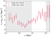 |
Fig. A.1. Reproduction of the LOWZ measurement from Si15 for validation purposes. While we recovered a 2% agreement on the number of galaxies in the shape sample, the signals are in excellent agreement on all scales above 0.5 Mpc. At small scales, the number of pairs becomes very small, which makes the measurement noisier. |
To validate our wgg estimation we were satisfied by reaching agreement on b1, b2 with Sa23. We also use this opportunity to validate our analytical covariance matrix against the jackknife matrix estimates from LOWZ, we show the result in Fig. A.2. As can be expected from the correlation function plot, the agreement is good on all scales.
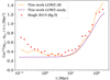 |
Fig. A.2. Validation of our covariance matrix estimate with the LOWZ sample from Reyes et al. (2012), Nakajima et al. (2012). We observe that our analytical prediction, the jackknife from Singh 2015, and our jackknife all agree very well, in particular on the scales of interest, while they deviate slightly below 1 Mpc. |
Appendix B: Comparison to Lensfit
While the catalogue produced by ShapePipe (Farrens et al. 2022) is the main UNIONS catalogue, a second catalogue was produced by lensfit to cross-check any systematics. For example it can be seen in Li et al. (2023) that both agree very well when measuring lensing masses of AGN-black holes. The strategy adopted in the lensfit pipeline is described in Miller et al. (2013). In short, the pipeline adopts a likelihood-based method by fitting a bulge+disk model in a Bayesian framework, which includes nuisance parameters, such as the galaxy position, which are marginalised over.
Although it was not used for the main results (as the catalogue was not fully validated by the time of this work), we nevertheless verified that a good agreement exists as can be seen in Fig. B.1, where the CMASS-UNIONS data vectors generated with lensfit and ShapePipe are in good agreement on all scales. While this is not a sufficient check to diagnose all systematics, it increases our confidence in our results.
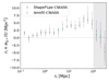 |
Fig. B.1. Comparison of lensfit and ShapePipe estimates of wg+. The good agreement increases confidence in the robustness of the measurement. |
We note that it is not necessary for the wg+ from the two different shape methods to be in agreement, as they are based on very different model-fitting functions. This is known to potentially result in different intrinsic alignment amplitudes, as explained throughout this paper. While we initially believed that we would be able to obtain further constraints from the comparison of these two shape measurement samples, recent work by MacMahon-Gellér & Leonard (2024) showed that a dedicated method was necessary to draw conclusions from a relative change in amplitude.
All Tables
Mean and standard deviations of the posterior distributions of the three parameters and the reduced χ2 values associated with the diagonal blocks of the covariance matrix.
Luminosity and intrinsic alignment amplitudes for the CMASS samples split into luminosity bins.
Table testing the compatibility with the null hypothesis of the different samples.
All Figures
|
Fig. 1. Distribution of the different spectroscopic and lensing samples used in this work. The plot on the left shows the North Galactic Cap (NGC), where most UNIONS galaxies lie. On the right is a portion of the South Galactic Cap (SGC), with the DES Y3 observations in the most southern part. There is no overlap between the UNIONS and DES Y3 catalogues. The apparent variation in shades between the two panels is due to the two projections resulting in different point densities. |
| In the text | |
|
Fig. 3. Un-weighted normalised r-band magnitude distributions of the BOSS/eBOSS spectroscopic samples and UNIONS photometric galaxies. We can see that the spectroscopic galaxies from the BOSS/eBOSS surveys fall into the brighter tail of the UNIONS distribution. The galaxies which dominate the lensing signal are comparatively fainter. Note: we could not use our large overlap with LOWZ galaxies as these bright galaxies (r < 20) are mostly absent from our lensing sample due to size cuts. |
| In the text | |
|
Fig. 2. Un-weighted normalised redshift distribution n(z) of the three BOSS/eBOSS galaxy samples. The UNIONS n(z) is approximate and for reference only, as blinding was implemented as a shift in the redshift distribution. The n(z) has been obtained by matching galaxies in the CFHTLenS W3 field and calibrated through deep spectroscopic reference samples. |
| In the text | |
|
Fig. 4. Square root of the diagonal of the analytical covariance matrix of wg+ for the CMASS-UNIONS sample (green solid line). The individual contributions are cosmic variance (dashed; the PggPII term is identical to the PgI contribution); mixed clustering – ellipticity shot noise (dotted); mixed intrinsic – density shot noise (long dash-dotted); and pure shot noise (short dash-dotted). See Eq. (42) and text for details. For comparison, we plot the jackknife variance (purple solid line), which is in excellent agreement with the analytical covariance over the relevant scales. |
| In the text | |
|
Fig. 5. Measurements of wg+ (upper panels) and w++ (lower row) for the UNIONS-CMASS (left), UNIONS-LRG (middle), and UNIONS-ELG (right column) samples. The solid lines show the best-fit NLA model, where the shaded areas indicate the 1σ uncertainty associated with the fit. The grey areas are excluded from the fit as explained in Sect. 4.7. |
| In the text | |
|
Fig. 6. Best-fit lines and 1σ contours for the NLA and TATT, respectively. The TATT model is fit down to 4 Mpc but both models appear very consistent. The 1σ TATT contours are obtained by drawing 500 models from the posterior and calculating the 68% confidence interval at eat rt. |
| In the text | |
|
Fig. 7. Posterior contours of the NLA and TATT model fitted to the CMASS-UNIONS sample. We see no deviation from the NLA case as A2 and bTA appear consistent with 0. |
| In the text | |
|
Fig. 8. Integrated correlation function, wg+, as measured on the CMASS-UNIONS sample split in 3 bins of luminosity, showing increasing luminosity from left to right panels. One can see a clear increase in the amplitude of the signal. |
| In the text | |
|
Fig. 9. Intrinsic alignment amplitude as a function of luminosity as measured by different surveys. The fitted function is α⟨L/L0⟩β. We can see very similar scaling with luminosity when comparing our CMASS-DES and CMASS-UNIONS measurements. |
| In the text | |
|
Fig. 10. 1D marginal posterior of the NLA intrinsic-alignment amplitude AIA of the same SDSS density tracer. Left panel: UNIONS, DES Y3 (both our measurements), and the results from Kurita & Takada (2023) in the North (NGC) and South Galactic Cap (SGC) using CMASS as density tracer. Right panel: Our measured UNIONS and DES Y3 results with the LRG sample. |
| In the text | |
|
Fig. 11. Measurements of wg× for the CMASS-UNIONS, LRG-UNIONS and ELG-UNIONS samples. Deviations from 0 are characterised in Table 4 and are all compatible at the 1σ level. |
| In the text | |
|
Fig. 12. Amplitude expressed by Eq. (50) of the additive bias contamination of the shape-shape correlation function. From left to right, we show our measurements using the Si15 data corresponding to the isophotal, de Vaucouleurs, and re-Gaussianisation shape catalogues, followed by UNIONS-CMASS, UNIONS-LRG, and UNIONS-ELG. |
| In the text | |
|
Fig. 13. Relative contribution to the wg+ signal of PSF induced correlations. We see that on the scales of interest the contribution is below 2% which we judge satisfactory for current precision. The error bars blow up when wg+ is close to 0. |
| In the text | |
|
Fig. A.1. Reproduction of the LOWZ measurement from Si15 for validation purposes. While we recovered a 2% agreement on the number of galaxies in the shape sample, the signals are in excellent agreement on all scales above 0.5 Mpc. At small scales, the number of pairs becomes very small, which makes the measurement noisier. |
| In the text | |
|
Fig. A.2. Validation of our covariance matrix estimate with the LOWZ sample from Reyes et al. (2012), Nakajima et al. (2012). We observe that our analytical prediction, the jackknife from Singh 2015, and our jackknife all agree very well, in particular on the scales of interest, while they deviate slightly below 1 Mpc. |
| In the text | |
|
Fig. B.1. Comparison of lensfit and ShapePipe estimates of wg+. The good agreement increases confidence in the robustness of the measurement. |
| In the text | |
Current usage metrics show cumulative count of Article Views (full-text article views including HTML views, PDF and ePub downloads, according to the available data) and Abstracts Views on Vision4Press platform.
Data correspond to usage on the plateform after 2015. The current usage metrics is available 48-96 hours after online publication and is updated daily on week days.
Initial download of the metrics may take a while.