| Issue |
A&A
Volume 699, July 2025
|
|
|---|---|---|
| Article Number | A314 | |
| Number of page(s) | 29 | |
| Section | Stellar atmospheres | |
| DOI | https://doi.org/10.1051/0004-6361/202553799 | |
| Published online | 21 July 2025 | |
X-Shooting ULLYSES: Massive stars at low metallicity
XIII. Testing the bi-stability jump in the Large Magellanic Cloud
1
Astrophysics Research Cluster, School of Mathematical and Physical Sciences, University of Sheffield,
Hicks Building, Hounsfield Road,
Sheffield
S3 7RH,
UK
2
School of Chemical, Materials and Biological Engineering, University of Sheffield,
Sir Robert Hadfield Building, Mappin Street,
Sheffield
S1 3JD,
UK
3
Institute of Astronomy, KU Leuven,
Celestijnenlaan 200D,
3001
Leuven,
Belgium
4
Departamento de Astrofísica, Centro de Astrobiología, (CSIC-INTA),
Ctra. Torrejón a Ajalvir, km 4,
28850
Torrejón de Ardoz, Madrid,
Spain
5
Armagh Observatory and Planetarium,
College Hill,
Armagh
BT61 9DG,
UK
6
Lennard-Jones Laboratories, Keele University,
Keele
ST5 5BG,
UK
7
Faculty of Physics, University of Duisburg-Essen,
Lotharstraße 1,
47057
Duisburg,
Germany
8
Zentrum für Astronomie der Universität Heidelberg, Astronomisches Rechen-Institut,
Mönchhofstr. 12–14,
69120
Heidelberg,
Germany
★ Corresponding author: This email address is being protected from spambots. You need JavaScript enabled to view it.
Received:
17
January
2025
Accepted:
1
June
2025
Abstract
Context Massive stars (>8 M⊙) play an important role in galactic evolution at all cosmic ages. A deeper understanding of the behaviour of mass loss in low metallicity environments is therefore required. This behaviour largely determines the path of a massive star throughout its life, and its final fate. A better understanding would allow us to predict the evolution of massive stars in the early Universe better.
Aims We investigated the theoretical bi-stability jump, which predicts an increase in the mass-loss rates below Teff ≈25–21 kK. We further constrained the photospheric and wind parameters of a sample of late-O and B supergiants in the Large Magellanic Cloud.
Methods We used the 1D non-local thermal equilibrium radiative transfer model CMFGEN in a grid-based approach and a fine-tuned spectroscopic fitting procedure that allowed us to determine the stellar and wind parameters of each star. We applied this method to ultra-violet data from the ULLYSES programme and to complementary optical data from the XShootU collaboration. We also used evolutionary models to obtain the evolutionary masses, and we compared them to the spectroscopic masses we derived.
Results We derived physical parameters and wind properties of 16 late-O and B supergiants that span a wide temperature range of Teff ≈12–30 kK, surface gravity range of log (g/cm s−2) ≈1.8–3.1, and mass-loss rate range of Ṁ ˙≈ 10−7.6−10−5.7 M⊙ yr−1. We also compared our results to previous studies that attempted to investigate the metallicity dependence of the wind properties.
Conclusions The photospheric and wind properties we derived are consistent with those of multiple previous studies. The evolutionary and spectroscopic masses for most of our sample are consistent within the uncertainties. Our results do not reproduce a bi-stability jump in any temperature range, but rather a monotonic decrease in the mass-loss rate at lower temperatures. We obtain a relation of the wind terminal velocity to effective temperature for supergiants in the Large Magellanic Cloud of ν∞/km s−1 = 0.076(±0.011)Teff/K − 884(±260). The mass-loss rates we derived disagree with the mass-loss rates predicted by any of the numerical recipes. This is also the case for the ratio of the terminal wind velocity to the escape velocity ν∞/νesc, and we derived the relation ν∞/νesc = 4.1(±0.8) log (Teff/K) −16.3(± 3.5). The wind parameters depend on the metallicity, based on a comparison with a previous study of the Small Magellanic Cloud, and the modified wind momentum-luminosity relation is log DmomLMC = 1.39(±0.54)log(Lbol/L⊙) + 20.4(±3.0).
Key words: techniques: spectroscopic / stars: massive / stars: mass-loss / supergiants / stars: winds, outflows
© The Authors 2025
 Open Access article, published by EDP Sciences, under the terms of the Creative Commons Attribution License (https://creativecommons.org/licenses/by/4.0), which permits unrestricted use, distribution, and reproduction in any medium, provided the original work is properly cited.
This article is published in open access under the Subscribe to Open model. This email address is being protected from spambots. You need JavaScript enabled to view it. to support open access publication.
1 Introduction
Massive stars (>8 M⊙) are hot and luminous stars with powerful winds that provide significant radiative, chemical, and mechanical feedback to their surroundings in every evolutionary stage. Because the mass loss via stellar winds is significant, the evolution of massive stars cannot be predicted solely by determining the initial mass. This means that the mass that is lost throughout the life of a massive star might make the difference between its life ending in a core-collapse supernova (ccSNe II/Ib/Ic) and leaving behind a black hole (BH) or a neutron star (NS), or a direct collapse into a BH without a ccSN (Smartt 2009).
Massive stars are rare by absolute numbers, but their high temperatures and, subsequently, their extreme ultra-violet (UV) fluxes are thought to have played an essential role in re-ionising the Universe (Haiman & Loeb 1997). Their ionising radiation may also drive star formation in their host galaxies (Crowther 2019).
Massive stars eject mass during all evolutionary stages via stellar winds. In the advanced evolutionary stages (supergiants), their stellar winds become more powerful than on the zero-age main sequence (ZAMS), leading to copious mechanical feedback to their surroundings (for a general review on massive star feedback see e.g. Geen et al. 2023).
The efficient internal mixing processes enrich these stellar winds in elements that were synthesised in the interior layers of the star (Langer 2012). This process plays an important role in the chemical enrichment of the inter-stellar medium (ISM), which in turn has a significant impact on the chemical evolution of the parent galaxy. The explosive nucleosynthesis in ccSNe yields elements heavier than iron, and this also drives the chemical evolution and metallicity Z of the host galaxy (Smith 2014).
Empirically derived stellar parameters accompanied by evolutionary (Yoon et al. 2006; Brott et al. 2011) and population synthesis models (Leitherer et al. 1999; Stanway & Eldridge 2018) can be used to study the collective evolutionary paths of massive stars. Thus, bridging the gap between the empirical and theoretically predicted properties of massive stars (Vink et al. 2001; Krtička et al. 2021; Björklund et al. 2023) is a fundamental pillar for an overall better understanding of the galactic evolution on a cosmic timeline.
Blue supergiants are the visually brightest stars in external galaxies (Bresolin et al. 2001). They have been used successfully as extragalactic distance indicators and diagnostics of heavy-metal metallicities (Kudritzki et al. 2003; Urbaneja et al. 2005a; Przybilla et al. 2006; Kudritzki et al. 2024).
The principal motivation for our study is to investigate the behaviour of the winds of late-O and B supergiants in the LMC, more specifically, in the temperature range associated with the bi-stability jump. The term bi-stability jump describes a phenomenon of a steep jump in stellar wind density around Teff ≈ 25–21 kK, and it was first coined by Pauldrach & Puls (1990) in a spectroscopic analysis of P Cygni in which two solutions were possible. The first solution has a high temperature (the “hot” side of the jump) and involved higher ionisation levels that would produce a faster and relatively low-density wind. The second solution had a lower temperature (the “cool” side of the jump), in which the wind recombines to lower ionisation stages. This results in a significant drop in the terminal velocity and in a denser wind. Later, Lamers et al. (1995) observed a jump in the ratio ν ∞ /νesc from ≈2.6 for supergiants earlier than B1 ( ≈ 25 kK) to ν ∞ /νesc ≈ 1.3 for supergiants of types later than B1 (Kudritzki & Puls 2000). The reason for this jump is attributed to the recombination of Fe IV to Fe III, as explained by Vink et al. (2000), since these lines dominate the acceleration in the subsonic part of the wind (Vink et al. 1999). Fe III has far more lines in the UV region close to the peak of the spectral energy distribution (SED) than Fe IV. Thus, more momentum is transmitted to the material, and a much higher mass loss is produced.
Vink et al. (2001) provided a numerically derived mass-loss prescription, where the temperature of the jump that divides the range into cool and hot depends on the Eddington parameter Γe and the metallicity. The introduction of the bi-stability jump might increase the mass-loss rate by a factor of seven for the cool compared to the hot solution for stars that are located roughly around the bi-stability jump.
On the other hand, newer mass-loss prescriptions using a different approach for calculating the radiative acceleration, such as Björklund et al. (2021) and Krtička et al. (2021), did not predict such a steep increase in the mass-loss rates. There have been multiple efforts to explore the behaviour of the wind of blue supergiants around the bi-stability jump in the Milky Way (Crowther et al. 2006; Benaglia et al. 2007; de Burgos et al. 2024a) and in the LMC (Verhamme et al. 2024) and SMC (Bernini-Peron et al. 2024).
This investigation is facilitated by the advent of the Ultra-violet Legacy Library of Young Stars as Essential Standard (ULLYSES, Roman-Duval et al. 2025), to which 1000 orbits of Hubble Space Telescope (HST) were dedicated, making this the largest HST Director’s Discretionary program ever conducted. ULLYSES compiled an ultra-violet (UV) spectroscopic Legacy Atlas of about 250 OB stars in low-Z regions, spanning the upper Hertzsprung-Russell diagram. The XShooting ULLYSES (XShootU) collaboration (Vink et al. 2023) also compiled a complementary optical spectral library of the same stars using the medium-resolution spectrograph X-shooter (Vernet et al. 2011) mounted on the Very Large Telescope (VLT). This complimentary dataset is referred to as Xshooting ULLYSES (XshootU). The ULLYSES and XShootU observations were not conducted simultaneously. Consequently, the impact of the time-dependent nature of stellar winds on non-photospheric spectral lines cannot be explored. This analysis can only be conducted with extensive time series of optical and UV spectra (see e.g, Markova et al. 2005; Massa et al. 2024).
Although several studies investigated the properties of OB supergiants in the Milky Way (MW, e.g., Herrero et al. 2002; Repolust et al. 2004; de Burgos et al. 2023) and the Magellanic Clouds (MCs, e.g., Crowther et al. 2002; Bestenlehner et al. 2020; Brands et al. 2022) using various analysis techniques, none of these studies had the unique ULLYSES/XshootU dataset. Unlike optical-only studies, the UV spectra of OB supergiants provide a deeper insight into the properties of the wind by allowing the direct measurement of wind velocities and the breaking of the mass-loss rate clumping degeneracy via saturated and unsaturated P Cygni profiles (Vink et al. 2023). This degeneracy has been extensively discussed in the literature. Simply spoken, optical wind diagnostics such as Hα or He II λ4686 (in the case of O supergiants) tend to overestimate the mass-loss rates when wind clumping is neglected (Puls et al. 2008). On the other hand, mass-loss rates that are estimated using unsaturated P Cygni profiles alone tend to have very large uncertainties because the wind lines are intrinsically highly variable (Massa et al. 2024), and they are subject to degeneracies because X-rays are generated via shocks in the wind (Puls et al. 2008).
In Section 2, we present a detailed account of the observational data that were used in the study. In Section 3, we describe the methods and techniques that were used in the analysis in detail. In Section 4, we present our results, including the values of the physical and wind parameters that were obtained through our pipeline. In Section 5, we compare our results to previous empirical studies and numerical predictions, and we discuss the implications of our findings on the bi-stability jump and the effect of metallicity on wind parameters. In Section 6, we summarise the interpretations of our results and discuss our plan for follow-up studies.
2 Observations
2.1 Sample
We initially chose a sample of LMC supergiants in the spectral type range O7-B9, the classification of which was obtained from various sources and compiled in Vink et al. (2023). In Table 1, we provide the updated spectral type taken from Bestenlehner et al. (2025), in which the classification was determined using O star templates from Sota et al. (2011) and B star templates from Negueruela et al. (2024). In the revised classification, the luminosity class of Sk −70◦ 16 was changed from a low luminosity supergiant (Ib) to a bright giant (II). During this study, we had to exclude some objects due to signs of binarity or odd features in the morphology of optical wind-lines (Hα and He II λ4686) that could hint toward a circumstellar discs, leaving the sample with objects in the spectral range O9-B8, covering a wide temperature range that includes the bi-stability jump (theoretically predicted to be around B1 spectral type). We briefly discuss the omitted objects in the supplementary online material on Appendix E.
Targets in our sample.
2.2 UV data (ULLYSES)
The UV data we used are a subset of the HST ULLYSES sample (Roman-Duval et al. 2025), which obtained moderate-resolution spectra of OB stars with selected wavelength settings of the Cosmic Origins Spectrograph (COS, Green et al. 2012) G130M/1291, G160M/1611 and G185M/1953 with resolutions R ≈12 000–16 000, R ≈13 000-20 000, and R ≈16 000–20 000 respectively, and the Space Telescope Imaging Spectrograph (STIS, Woodgate et al. 1998) E140M/1425 (R ≈ 45 800), and E230M/1978 (R ≈30 000) gratings in the far- and near-UV during HST cycles 27–29. Those new spectra were combined with suitable existing spectra (previously obtained with FUSE and/or HST). Far Ultra-violet Spectroscopic Explorer (FUSE) spectra cover the wavelength ≈900–1160 Å through the 4′′ × 20′′ (MDRS) or 30′′ × 30′′ (LWRS) appertures, with a resolving power of ≈15 000 (Moos et al. 2000).
2.3 Optical data (XShootU)
To complement the UV spectra, high quality optical/NIR spectroscopy was carried out with the X-shooter instrument (Vernet et al. 2011), which is mounted on the Very Large Telescope (VLT). This slit-fed (11′′ slit length) spectrograph provides simultaneous coverage of the wavelength region between 3000– 10 200 nm, across two arms; UVB (300 ≤ λ ≤560 nm), VIS (560 ≤ λ ≤ 1000 nm). X-shooter’s wide wavelength coverage made it the instrument of choice to build an optical legacy data-set (Vink et al. 2023). The XshootU dataset was observed with the following settings: 0.8′′ slit width for the UBV arm achieving spectra resolution R ≈ 6700, and 0.7′′ for the VIS arm (R ≈11 400). Fig. 1 shows the optical spectra, which were combined, flux calibrated, corrected for telluric contamination, and normalised by Sana et al. (2024, DR).
2.4 Auxiliary data (MIKE)
Another complementary spectroscopic optical dataset was collected using the Magellan Inamori Kyocera Echelle (MIKE) spectrograph, which is mounted on the Magellan Clay Telescope, for known slow rotating ULLYSES stars. The higher spectral resolution (R ≈ 35 000–40 000) and the wide wavelength coverage (3350–5000 Å blue arm) and (4900–9500 Å red arm) is needed to resolve spectral features and determine their rotation rates using metal lines (Crowther 2024). Four of the stars in our analysed sample are also included in the Magellan/MIKE sample Sk −67◦ 78, Sk −70◦ 16, Sk −68◦ 8, and Sk −67◦ 195.
2.5 Photometry
The photometric magnitudes we used in the SED fitting to obtain the bolometric luminosities of the targets were taken from various sources and compiled in Vink et al. (2023). The UBV photometry are drawn from Ardeberg et al. (1972); Schmidt-Kaler et al. (1999); Massey (2002).
The infrared JKS photometry are preferably taken from the VISTA near-infrared YJKS survey of the Magellanic System (VMC, Cioni et al. 2011), with H-band photometry taken from the Two Micron All Sky Survey (2MASS, Cutri et al. 2003; Skrutskie et al. 2006). For very bright sources that are saturated in VMC (Cioni et al. 2011) we use the J and KS photometry provided in 2MASS (Skrutskie et al. 2006).
2.6 UV normalisation
The UV spectra require normalisation, which is challenging due to the iron forest that heavily contaminates the continuum. Fig. 2 shows normalised UV spectra of a subset of our sample. The quality of the fits to the UV lines is highly dependent on the quality of the normalisation of the observed spectrum. On average, we obtained very good normalised UV and far UV spectra for the targets by using the SED fitting explained later in Section 3.4.3 to obtain the bolometric luminosities of the targets. In essence, we apply the extinction from Gordon et al. (2003) to the normalised synthetic spectrum of the best-fitting model and scale it to the flux levels of the observed spectrum using the KS magnitude, then simply divide the observed spectrum by the extinct and scaled continuum of the model to obtain a normalised spectrum with relative flux values.
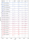 |
Fig. 1 Normalised XshootU spectra (Sana et al. 2024, DR1) in the blue optical range of the sample with identifications for a subset of the optical lines. For illustration purposes, we added an arbitrary offset of 0.5 for each spectrum. The fits to the violet, yellow, and red spectra for all stars are presented in Appendix I. |
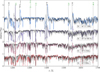 |
Fig. 2 Normalised UV spectra in the range of the sample, with the line identification for the UV lines. For illustration purposes, an offset of one was added. The coloured lines show the observations. The black lines show the model fits for each of the respective stars. Stellar features are indicated in black line labels, whereas green line labels indicate interstellar features. The HST gap at ≈1300 in the spectra of Sk 69◦ 52, Sk 68◦ 8 is due to appending observations from COS G130M and COS G160M. The gap at 1600 Å is due to appending observations from COS G160M and COS G185M. Other UV fits are presented at Appendix I. |
3 Method
Line-blanketed plane-parallel model atmospheres such as TLUSTY (non-LTE, Hubeny & Lanz 1995) and ATLAS (LTE, Kurucz 1979) coupled to SURFACE/DETAIL (Butler & Giddings 1985) have been widely applied to early-type stars with weak winds to derive physical parameters and accurate elemental abundances (e.g., Przybilla et al. 2006; Hunter et al. 2007; Przybilla et al. 2008). This combined non-LTE method has been also been recently employed in studies of B supergiants (e.g., Weßmayer et al. 2022, 2023). For stars with strong stellar winds, it is necessary to employ line-blanketed model atmospheres with spherical geometry. Examples include FASTWIND (Puls et al. 2005; Rivero González et al. 2012), POWR (Gräfener et al. 2002; Hamann & Gräfener 2003) and CMFGEN (Hillier 1990; Hillier & Miller 1998). These codes have the advantage of incorporating stellar winds, albeit at the expense of computational resources, such that the determination of physical parameters and elemental abundances are more costly than the plane-parallel case.
3.1 Model atmosphere code and grid
We used the code CMFGEN (Hillier 1990; Hillier & Miller 1998), which solves the radiative transfer equations in a 1-D non-LTE, spherical geometry with a radial outflow of material (that can also be optically thick in the continuum) in the co-moving frame. We chose to use CMFGEN because it accounts for the influence of extreme-UV line blanketing on the wind populations and ionisation structure that is the result of thousands of overlapping lines. It does that with a detailed treatment using super-levels, which was pioneered by Anderson (1985, 1989), in which several levels with similar energies and properties are treated as a single or super level. The idea of super-levels is of tremendous importance for the iron-group elements. An individual ionisation stage can have hundreds of levels and line transitions (cf. the iron forest in Fig. 2) that need to be considered in the full model atom, but applying the super-levels method significantly reduces the number of statistical equilibrium equations to be considered in the NLTE treatment. There is also a time-dependent variant of CMFGEN for the simulation of supernovae spectra (e.g., Dessart & Hillier 2010), but the scheme we employed assumes stationary outflows.
For the initial setup of the (quasi-)hydrostatic layers, a previous CMFGEN model can be used. CMFGEN does not calculate the velocity field stratification with the radiative acceleration. Instead, the density (velocity) structure of the extended atmosphere is set through the continuity equation by a parametrised velocity law ν(r) on top of a solution of the hydrostatic equation from a connection velocity to the inner photosphere (e.g., Martins et al. 2012).
In CMFGEN, clumping is treated in the optically thin clumping approximation, also known as “micro-clumping”, assuming a void inter-clump medium and a volume-filling factor fvol. To solve the radiative transfer equation with the micro-clumping assumption, the size of the clumps is assumed to be smaller than the mean free path of the photons (Hillier 1996). The treatment of wind inhomogeneities in CMFGEN has been extensively discussed in the literature (Hillier 1997; Hillier & Miller 1998, 1999). In the grid, we adopt a velocity-dependent clumping law that was introduced for O stars in Hillier et al. (2003)
![Mathematical equation: \[f(r) = {f_{{\rm{vol}},\infty }} + \left( {1 - {f_{{\rm{vol}},\infty }}} \right){\rm{exp}}\left( { - \frac{{v(r)}}{{{v_{{\rm{cl}}}}}}} \right),\]](/articles/aa/full_html/2025/07/aa53799-25/aa53799-25-eq3.png) (1)
where fvol, ∞ is the terminal volume-filling factor, νcl is the onset clumping velocity, and ν(r) is the velocity of the wind at a given radius r. In its essence, fvol,∞ determines the degree of clumping in the wind, where smaller values of fvol,∞ indicate a more highly clumped wind at r → ∞. νcl determines the location (depth) at which clumping starts. This means that Equation (1), describes winds that become smoother as ν(r) becomes lower approaching the photosphere, and become rapidly more clumped at larger radii. In our grid, we fix fvol,∞ to a value of 0.1. Later in the fine-tuning procedure, fvol, ∞ is treated as a free parameter. This is essential for obtaining satisfactory fits for the electron scattering wings of Hα and unsaturated P Cygni resonance lines.
(1)
where fvol, ∞ is the terminal volume-filling factor, νcl is the onset clumping velocity, and ν(r) is the velocity of the wind at a given radius r. In its essence, fvol,∞ determines the degree of clumping in the wind, where smaller values of fvol,∞ indicate a more highly clumped wind at r → ∞. νcl determines the location (depth) at which clumping starts. This means that Equation (1), describes winds that become smoother as ν(r) becomes lower approaching the photosphere, and become rapidly more clumped at larger radii. In our grid, we fix fvol,∞ to a value of 0.1. Later in the fine-tuning procedure, fvol, ∞ is treated as a free parameter. This is essential for obtaining satisfactory fits for the electron scattering wings of Hα and unsaturated P Cygni resonance lines.
Fig. 3 shows a slice of the grid in Teff-log g space. We fixed the luminosity in our models to log (L/L⊙) = 5.8 and varied log (Teff/K) in the range ≈ [4.15, 4.60] and log (g/cm s−2) in the range ≈ [1.7, 3.9] depending on the temperature, in steps of 0.025 dex for log (Teff/K) and 0.2 dex for log (g/cm s−2). We employed the empirical temperature and metallicity dependent terminal wind velocity recipe from Hawcroft et al. (2024)
![Mathematical equation: \[{v_\infty }\left( {{\rm{km\;}}{{\rm{s}}^{ - 1}}} \right) = \left[ {0.092( \pm 0.003){T_{{\rm{eff\;}}}}({\rm{K}}) - 1040( \pm 100)} \right]Z/Z_ \odot ^{(0.22 \pm 0.03)},\]](/articles/aa/full_html/2025/07/aa53799-25/aa53799-25-eq4.png) (2)
where Z ≈ 0.43Z⊙ for the LMC (Choudhury et al. 2016). In Hawcroft et al. (2024), Sobolev with Exact Integration (SEI) modelling was employed to measure the terminal wind velocities for objects no later than B1.5 spectral types, using the C IV λλ1548–1551 resonance doublet, with radial velocities adopted from the UV.
(2)
where Z ≈ 0.43Z⊙ for the LMC (Choudhury et al. 2016). In Hawcroft et al. (2024), Sobolev with Exact Integration (SEI) modelling was employed to measure the terminal wind velocities for objects no later than B1.5 spectral types, using the C IV λλ1548–1551 resonance doublet, with radial velocities adopted from the UV.
In our grid, we used the modified β velocity law that was introduced by Hillier et al. (2003)
![Mathematical equation: \[v(r) = {v_0} + \left( {{v_\infty } - {v_0}} \right){\left( {1 - \frac{{{R_ * }}}{r}} \right)^\beta },\]](/articles/aa/full_html/2025/07/aa53799-25/aa53799-25-eq5.png) (3)
where ν ∞ is the terminal wind velocity, ν0 is the connection velocity, which is estimated as two thirds the speed of sound ≈10 km s−1, and Rτ=100 is the radius of the star, which is defined at optical depth τ = 100. For our grid, we adopt a fixed value of β = 1. This procedure yielded a 2-D grid in the temperature-gravity parameter space (gridbase).
(3)
where ν ∞ is the terminal wind velocity, ν0 is the connection velocity, which is estimated as two thirds the speed of sound ≈10 km s−1, and Rτ=100 is the radius of the star, which is defined at optical depth τ = 100. For our grid, we adopt a fixed value of β = 1. This procedure yielded a 2-D grid in the temperature-gravity parameter space (gridbase).
In Table 2, we present the values of metal abundances log X/H + 12 (by number) adopted in the model grid. Hence-forth, we substitute log X/H + 12 with the notation ϵX. Rather than adopting baseline LMC CNO abundance values for metals such as the one compiled in Vink et al. (2023), we chose to adopt processed abundances correlating to low luminosity B stars in the LMC from Hunter et al. (2008), that show nitrogen enhancement of ΔϵN ≈+0.47 dex, compared to the LMC baseline in Vink et al. (2023), and at the expense of carbon and oxygen deficiencies of ΔϵC ≈−0.5 dex and ΔϵO ≈ − 0.07 dex. Since Hunter et al. (2008) excludes B supergiants, we checked the validity of these values for luminous B supergiants (which might be expected to show the greatest N enhancements) by resorting to the work of McEvoy et al. (2015), in which TLUSTY non-LTE model atmosphere calculations have been used to determine atmospheric parameters and nitrogen abundances for 34 single and 18 binary supergiants. Their analysis shows a nitrogen enrichment value of ≈ 0.5 dex relative to Vink et al. (2023), which is very close to our grid’s nitrogen abundance. For other key elements in our grid like silicon, magnesium, and iron, we implemented baseline LMC abundances from Vink et al. (2023). Abundances of metals heavier than oxygen are not modified during the fitting procedure.
Lastly, we covered the temperature-gravity-wind density parameter space. We did that by iterating over the mass-loss rates  in the range ≈ [ − 5.5, − 7.3] in steps of 0.3 dex for each of the points from gridbase. The final grid is a 3-D grid in the temperature-gravity-wind density space.
Since the strength of emission features scales not only with the mass-loss rate but also with the volume-filling factor ( fvol), terminal velocity, and radius of the star, it is convenient to compress these parameters into one parameter when compartmentalising the model grids. To spectroscopically quantify mass-loss rates of hot massive stars using scaling relations, we chose to adopt the transformed radius (Schmutz et al. 1989)
![Mathematical equation: \[{R_t} = {R_ * }{\left[ {\frac{{{v_\infty }}}{{2500\,{\rm{km\;}}{{\rm{s}}^{ - 1}}}}/\frac{{\dot M}}{{{{10}^{ - 4}}{M_ \odot }{\rm{y}}{{\rm{r}}^{ - 1}}\sqrt {{f_{{\rm{vol}}}}} }}} \right]^{2/3}},\]](/articles/aa/full_html/2025/07/aa53799-25/aa53799-25-eq9.png) (4)
which was originally used for optically thick winds of Wolf– Rayet stars (WR), where the line equivalent width is preserved. The grid covers a wide range of log Rt from 1.6 to 3.1, with lower values relating to denser winds. This log Rt range corresponds to an optical depth-invariant wind-strength parameter
(4)
which was originally used for optically thick winds of Wolf– Rayet stars (WR), where the line equivalent width is preserved. The grid covers a wide range of log Rt from 1.6 to 3.1, with lower values relating to denser winds. This log Rt range corresponds to an optical depth-invariant wind-strength parameter  (Puls et al. 1996) range of −13.9 to −11.5, where larger values of log Q correspond to denser winds. We employ Rt to scale
  to the derived bolometric luminosity of the star.
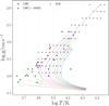 |
Fig. 3 Grey triangles show the model grid, purple squares show LMC targets with temperatures ≤ 40 kK (from the literature), and green points show LMC targets with temperatures ≥40 kK. The overlaid lines are isochrones taken from Brott et al. (2011). |
Metal abundances adopted in the model grid.
3.2 Atomic data and X-rays
We included 14 species and 50 different ions in our models. We excluded higher ionisation stages for the cooler (<25 kK) models and included the lower ionisation stages. This is of special importance to the iron lines, which dominate the UV in the B star regime. We include our detailed underlying model atom structure in the appendix in Table C.1.
X-rays can be included in CMFGEN using X-ray emissivities from collisional plasma models (Smith et al. 2001), where the source of this emission is assumed to be shocks forming in the winds (Pauldrach et al. 1994). The detailed approach used in CMFGEN is described in Hillier & Miller (1998). The general spectral appearance is not affected by X-rays, although the highest ionisation UV lines can be enhanced at the expense of lower ionisation lines (Baum et al. 1992) at relatively low stellar temperatures due to Auger processes. We elect to exclude X-rays from our analysis, because the ad hoc addition of X-rays in CMFGEN does not provide a phenomenological description of the physical shock parameters and reduces the number of unconstrained parameters in the fitting procedure.
The main drawback of excluding X-rays in our models is that, in some cases, it is difficult to obtain satisfactory fits for high ionisation UV P Cygni lines. This could potentially lead to overestimating the mass-loss rates. Bernini-Peron et al. (2023), who included X-rays in their CMFGEN models, found that their mass-loss rates for Galactic B supergiants are lower by a factor of two compared to the mass-loss rates obtained by Crowther et al. (2006) and Searle et al. (2008), who exclude X-rays. In Fig. 2, the discrepancy between the predicted and observed P Cygni N V λλ1238–1242 line in Sk − 66◦ 171 is due to the lack of X-rays in the model. This is also the case for the P Cygni C IV λλ1548–1551 profile in Sk −68◦ 140 and Sk −69◦ 52.
3.3 Summary of the fitting procedure
Since CMFGEN is time and resource-intensive, we are limited by a small number of models relative to the number of parameters that we have to extract from the stellar spectra. Therefore, as a first-order approximation (initial pinpoint), we use the results of the analysis done using the pipeline that was introduced in Bestenlehner et al. (2024), which is a grid-based χ2-minimisation algorithm that uses the entire optical spectrum rather than selected diagnostic lines. This allows us to analyse a wider range of temperatures from B to early-O stars. This grid of synthetic spectra was computed with the non-LTE stellar atmosphere and radiative transfer code FASTWIND (Puls et al. 2005), which is efficient and quick but lacks a detailed treatment of the iron forest in the UV range. This pipeline provides a first approximation of Teff, log g, νrot sin i using only the optical XShootU data, which we then can refine using the UV range provided by our CMFGEN grid, and then produce a fine-tuned model for the entire spectrum based on the best fitting grid model. To summarise, our entire procedure consists of the following steps:
1st step: Approximation of Teff and log g from the optical spectrum using the model de-idealisation pipeline introduced in Bestenlehner et al. (2024), which we use to pin-point the closest fitting model from the grid in
 parameter space.
2nd step: Fine-tune the values of Teff, log g, ν ∞ and the helium abundance of the model from the previous step.
3rd step: Fine-tune wind parameters
 , β-law, fvol and clumping on-set velocity νcl.
4th step: Refine CNO-surface abundances.
The second, third and fourth steps take on average ten tailored models in total to obtain a satisfactory fit.
3.4 Diagnostics
Underlying systematic errors arise from our grid and fitting procedure. The most notable are the inclusion of a limited number of species and ions, fixing certain parameters like the micro- and macro-turbulent velocities, and fixing the abundances of elements heavier than oxygen. An important part of our analysis is wind clumping, which can vary greatly depending on the treatment used in the model (e.g., Brands et al. 2022). Finally, the finite spectral resolution of the observation adds another layer of uncertainty to the overall analysis. We estimate the model uncertainties (parameters with superscript notation ‘m’), the derived physical parameters and wind properties. By ‘model uncertainty’ we simply mean the smallest variation in a given input parameter that would produce a noticeable change in the quality of the fit.
3.4.1 Effective temperature and helium abundance
After we derived a rough estimate of the stellar and wind parameters from our grid, we started fine-tuning the model parameters to reproduce the observed spectrum. In order to do that, we first vary the temperature, which has a large impact on the morphology of the spectrum for different spectral classes. Consequently, obtaining an accurate temperature determines the overall quality of the fit and of the other estimated stellar and wind parameters. In our fitting procedure, Teff is derived using the ionisation balance of helium (He) and silicon (Si). In practice, lines from successive ions, of the same elements must be observed.
The most reliable lines for O stars are He II and He I, and historically He II λ4542 and He I λ4471 have been used (Martins 2011), which is what we used for the O stars in our sample as primary diagnostics. Additionally we use He II λ5411 and He I λ4922 as a sanity check.
For B stars, the main diagnostic is the silicon ionisation balance (McErlean et al. 1999; Trundle et al. 2004; Trundle & Lennon 2005). For the earliest B stars (B0–B2) spanning a temperature range Teff ≈28–21 kK we use Si IV λλ4089–4116 1 and Si III λλλ4553–4568–4575 as our main diagnostics. For mid-B stars (B3-B5) in the temperature range Teff ≈20–14 kK Si III λλλ4553–4568–4575 and Si II λλ4128–4131 are used. For late-B stars (B6–B8), we resort to fitting He I λ4471 and Mg II λ4481, which is not as reliable as fitting consecutive ions of the same species.
An alternative indicator of Teff in late-B stars is the ratio of O II to O I line. By way of example, in Fig. 4 we show the triplet O I λλλ7772–7774–7775 (upper panel) and O II λ4254 (lower panel). The preferred model (red solid line) for the B8 super-giant Sk − 67◦ 195, the temperature of which was obtained from fitting He I λ4471 and Mg II λ4481, reproduces the O I λλλ7772– 7774–7775 and O II λ4254 lines relatively well. For comparison, we display another model that differs from the preferred model only in its temperature with ΔTeff = 1500 K (blue solid line). We select this model as it is the nearest model on the grid to our preferred model in the temperature parameter-space that presents O II lines. This fit implies that decreasing the oxygen abundance in the comparison model could produce a better match to both lines. This could be used either as a primary diagnostic for Teff or as a sanity check in late-B supergiants.
By way of a sanity check, we compared the predicted Balmer jump strengths to observations (Kudritzki et al. 2008; Urbaneja et al. 2017). We find that, for the most part, the strength of the predicted Balmer jumps – the Teff of which was obtained from line diagnostics – are in good agreement with observations. Nevertheless, a few hundred K higher temperatures produce a better match for a subset of mid- to late-B supergiants, albeit within the quoted uncertainties.
The earliest B stars (B0–B0.7) in the temperature range Teff ≈25–22 kK show weak He II lines, so we use He I λ4471 and He II λ4542 as a sanity check when fine-tuning the temperature for such objects. There is also a temperature range Teff ≈ 20–17 kK at which silicon lines of all three ionisation stages (Si IV, Si III, and Si II) are present. In those cases, we attempted to fit all lines but focused mainly on the stronger consecutive pair.
Since silicon is an alpha-process element, its abundance is primarily determined by the environment, so is not heavily influenced by the evolution of the star in the supergiant phase. Moreover, Korn et al. (2005) obtained a value of ϵSi = 7.07 ± 0.3 from fast-rotating B stars in the LMC, and Hunter et al. (2007) reported a silicon abundance ϵSi = 7.19 ± 0.07 from narrow-line late-O and B stars in the LMC, whereas Dopita et al. (2019) derived a value ϵSi = 7.11 ± 0.04 from supernova remnants in the LMC. The low variance between these values caused us to fix the silicon abundance. For those reasons, we did not attempt to fit the silicon line strength by changing the abundance of silicon at the fine tuning stage. We also do not change the abundance of magnesium during our fine tuning stage. Similar to silicon, this is motivated by the low variance between the magnesium abundance values obtained via different methods in the literature. ϵMg values from the literature are as follows: ϵMg = 7.15 ± 0.3 from Korn et al. (2005), and ϵMg = 7.06 ± 0.09 from Hunter et al. (2007), and ϵMg = 7.19 ± 0.09 from Dopita et al. (2019).
For O stars, the helium abundance is essential for an accurate temperature estimate. Changing the helium abundance at the expense of hydrogen modifies the ionisation structure in the atmosphere, which, in turn, affects the shape and strength of Hα, especially when it is in emission. This is the case for the majority of the targets in our sample. It is therefore important to also obtain an accurate helium abundance for the O and B stars. In our fitting procedure, as we are fitting temperature line diagnostics, we simultaneously fine-tune abundances of helium and hydrogen before attempting to fit wind lines such as Hα.
It is important to understand that varying Teff by small amounts can have a different effect on the quality of the fit depending on the temperature range of the model. To illustrate this, we show in Fig. 5 the effect of varying the temperature of the best fitting model (red solid line) by ΔTeff = − 700 K with all other parameters fixed. The top panels shows the fits to He II λ4542 and He I λ4471 (panels a and b respectively in Fig. 5) for the O9.5 Ib supergiant Sk − 71◦ 41, where the best fitting model has a Teff = 29.2 kK and we can see that while the model with lower temperature does not yield a noticeably different fit for He I λ4471, He II λ4542 is significantly changed. The equivalent widths (EW) ratio of He I λ4471 to He II λ4542 in the observations is ≈ 3.20 ± 0.05. our preferred model yield an EW ratio of ≈3.15 ± 0.05 compared to an EW ratio ≈3.45 ± 0.05 for the comparison model with the higher Teff.
Panels c and d in Fig. 5 show the comparison of the fits of Si IV λλ4088–4116 and Si III λλλ4553–4568–4575, respectively, for the B0 Ia supergiant Sk − 68◦ 52 (best fitting model Teff = 26.0 kK). In this case, lowering the temperature by ΔTeff = 700 K slightly worsens the quality of the fits for both sets of lines. The EW ratio of Si III λ4552 to Si IV λ4088 in the observed spectrum of Sk −68◦ 52 is ≈0.55 ± 0.05. Our preferred model yields an EW ratio of ≈0.51 ± 0.05 compared to an EW ratio of 0.45 ± 0.05 for the comparison model with the lower Teff.
In panels e and f of Fig. 5, we show the fits of the B3 Ia supergiant Sk − 67◦ 78 for Si III λλλ4553–4568–4575 and Si II λλ4128–4131, respectively, where the best fitting model has Teff = 15.5 kK. We can see that raising the temperature of the model by ΔTeff = 700 K noticeably deteriorates the quality of the fit. The EW ratio of Si II λ4128 to Si IV λ4552 in the observed spectrum of Sk − 67◦ 78 is ≈0.60 ±0.05. Our preferred model yields an EW ratio of ≈0.62 ± 0.05 compared to an EW ratio ≈0.53 ± 0.05 for the comparison model with the higher Teff.
We estimate the model uncertainty from the spectral fitting as  depending on the quality of the fit, and we estimate a more conservative and realistic uncertainty as double the model uncertainty in attempt to take into account limitations of the model atmosphere code, giving us ΔTeff ≈ ±1000–2000 K.
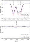 |
Fig. 4 O I λλλ7772–7774–7775 and O II λ4254 lines of the B8 super-giant Sk − 67◦ 195 (black line). Red line: the preferred model the temperature of which (Teff = 12.5 kK) was obtained from fitting He I λ4471 and Mg II λ4481, and a comparison with higher Teff = 14.0 kK. |
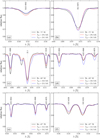 |
Fig. 5 Examples of the effect of varying Teff on the quality of the fit. The best-fitting model is shown with the solid red line. Comparison model: blue solid line (ΔTeff = 700 kK). Observed XShootU spectrum: black solid line. (a, b) Sk −71◦ 41 (O9.5 Ib). (c, d) Sk −68◦ 52 (B0 Ia). (e, f) Sk −67◦ 78 (B3 Ia). |
3.4.2 Effective surface gravity
The surface gravity (log g) is obtained via fitting the wings of Balmer lines. Balmer lines are broadened by collisional processes and are most sensitive to Stark broadening (linear Stark broadening affects the wings of the H and, to a lesser extent, He II lines; indeed, this effect is mainly used to constrain the surface gravity), which is related to gas pressure, and in turn, gas pressure is intimately connected to electron pressure (Pe = NeKT ) in hot stars. This means that Balmer lines are broader in higher gravity stars. Degeneracies that occur when fitting Balmer lines are alleviated once temperature diagnostic lines are included (fitting log g and Teff simultaneously and iteratively).
We use Hγ as the main indicator since it is usually in absorption and its wings are mostly not contaminated by wind emission or by blending with other lines. Hη and Hζ are used as a sanity check. These Balmer lines are usually strong and well resolved (Simón-Díaz 2020; Martins 2011), but in the case of the O hypergiants Sk − 68◦ 135 and Sk −69◦ 279 we resorted to fitting Hη as our primary surface gravity diagnostic due to wind contamination in all the lower Balmer lines.
To show the level of sensitivity of the model to modest changes in log g, we present two cases of fitting Hγ. For the O9 Ia supergiant Sk − 66◦ 171 (panel (a) in Fig. 6), the best fitting model (red solid line) was computed with log (g/cm s−2) = 3.05 dex and the comparison model (blue solid line) with log (g/cm s−2) = 3.10 dex. Both models were computed with the same Teff = 29.9 kK and with all other parameters kept the same, and as shown the two fits are very similar. The second case (panel (b) in Fig. 6) is for the B0 Ib supergiant Sk − 67◦ 5, where the best fitting model and the comparison model were computed for log (g/cm s−2) = 2.8 dex and 2.9, respectively, and the same Teff = 25.6 kK. In contrast to the previous case, a Δ log (g/cm s−2) = 0.1 dex dramatically changes the quality of the fit.
We estimate the model uncertainty at Δ log gm = ± 0.05– 0.10 dex and adopt a conservative uncertainty Δ log gc = ± 0.2– 0.25 dex which takes into account the additional uncertainty of νrot sin i and R* and the quality of the normalisation (a 1% change in the wings due to normalisation can lead to a log g difference of 0.1 dex).
3.4.3 Luminosity
For the determination of the bolometric luminosities Lbol of our stars, we use the flux from the model computations, which was computed for a fixed luminosity of log (Lmodel/L⊙ ) =5.8. We select the Vega magnitude system photometric zeropoint. First, we apply suitable filter functions from PYPHOT (Fouesneau 2025) using the effective wavelengths of the filters, and we obtain the BVKS fluxes of the model using the function get_ flux, and from the fluxes we calculate magnitudes of the model (Bm, Vm and  ) as
) as  . The filter function properties and Vega magnitudes are presented in Table 3. We then apply the extinction law from Gordon et al. (2003) and fit the relative extinction RV and other parameters that determine the shape of the UV extinction curve (Fitzpatrick & Massa 1990) to match the shape of the observed SED. The model SED is then scaled to the observed SED using a factor equal to
  . Using the model magnitudes, the colour excess E(B − V) is calculated as (B − V) − (Bm − Vm). Assuming the distance modulus DM for the LMC is 18.50 ± 0.02 mag (Alves 2004), we calculate the bolometric correction of the visual magnitude of the model
  with the equation
  . Finally, the bolometric luminosity is calculated via
  and the apparent visual magnitude of star m V as
  , where A V is the total extinction and is equal to E(B − V) RV. The absolute visual magnitude is calculated as MV = mV −DM − AV.
With this procedure, we simultaneously obtain the extinction parameter RV and the colour excess E(B − V). This method relies on the relation of the B and V bands to the KS band, and since the extinction is minimal in the KS, the obtained bolometric luminosities are highly reliable. The uncertainty of the derived bolometric luminosity is dominated by the uncertainty in the distance to the target, for which we adopt a random error of 0.1 dex. Additionally, the SED fitting method (by eye) results in an uncertainty in the AV, which is inherited by the bolometric luminosity. Finally, the 2MASS photometry formal errors range from 0.01 to 0.1, averaging ≈ 0.05. Therefore, we estimate the uncertainty to be ΔLbol ≈ ± 0.1–0.2 dex. The SED fits for the stars in our sample are presented in Appendix G.
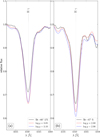 |
Fig. 6 Examples of the effect of varying log g on the quality of the fit. The best-fitting model is shown with the solid red line. Comparison model: blue solid line. Observed XShootU spectrum: black solid line. a: Sk −66◦ 171 (O9 Ia) (Δ log g = 0.05). b: Sk −67◦ 5 (B0 Ib) (Δ log g = 0.1). |
Properties of the PYPHOT filter functions (Fouesneau 2025).
3.4.4 Line-broadening parameters
Out of all parameters that cause spectral line-broadening (macro-turbulent velocity νmac, micro-turbulent velocity νmic, and projected rotational velocity νrot sin i) we elected to include only νrot sin i as part of the fitting procedure. When calculating the formal integral using CMFFLUX, we fix the νmic in the photosphere to 10 km s−1 and the maximum νmic in the wind to 100 km s−1.
Changing νmic in the photosphere has little effect on wind lines, but the changes in line opacities do affect photospheric lines (primarily metal but also He I lines). This produces a degeneracy between νmic and chemical abundances. Therefore, increasing νmic could lead to an underestimation of the abundances and temperatures (Brands et al. 2022), and we therefore excluded νmic from our fitting procedure. This degeneracy can be alleviated by simultaneously fitting νmic and the abundances using multiplet lines. A common diagnostic of νmic in B stars is the depth of the components of Si III λλλ4553–4568–4575, which are sensitive and react differently to changes in νmic (McErlean et al. 1998).
The values of macro-turbulent velocities on OB stars range from a few km s−1 for dwarfs up to a few tens of km s−1 for supergiants. We fix νmac at 20 km s−1 in our fitting procedure. Fixing νmac is appropriate for our sample, especially when taking into account the velocity resolution of the UBV and VIS arms of X-shooter that ≈ 45 and 25 km s−1, respectively. The main diagnostic line for O stars is O III 5592. For early-B stars O III 5592 is also used and as a sanity check we fit C III λ4267, Si IV λλ4089– 4116, and Si III λλλ4553–4568–4575. for mid- to late-B stars we fit the Mg II 4481 line and as a sanity check we use C II and Si II. The uncertainty in νrot sin i measurements is dominated by the velocity resolution of the UBV arm of X-shooter (Vernet et al. 2011) Δν ≈ 45 km s−1. Later in Section 4.4, we investigate the line-broadening characteristics of a subsample of our stars that have MIKE data by using the IACOB-BROAD tool (Simón-Díaz & Herrero 2014).
3.4.5 Terminal wind velocity (ν∞)
The black velocity νblack is the velocity measured at the bluest extent of fully saturated P Cygni absorption (Prinja et al. 1990). This is thought to provide a more robust estimate of the wind terminal velocity than the edge velocity νedge, which is measured at the point where the blue trough of the P Cygni profile intersects the local continuum (Beckman & Crivellari 1985). The difference νedge − νblack arises from the turbulence in the velocity field of the wind.
We obtained νedge and νblack using direct measurements of all the viable P Cygni resonance lines in the range ≈ [1200, 2900] Å, with the advantage of accurate radial velocity estimates for each object from the optical metal lines. νedge and νblack were determined as the mean value of all velocities obtained from the individual resonance lines. The resonance lines used are Si IV λλ1394–1403, C IV λλ1548–1551, Al III λλ1855–1863, and Mg II λλ2796–2803.
Stars at low metallicity are well known for having absorption profiles that may not reach zero intensity, consequently it is sometimes not possible to obtain an accurate measurement of νblack, and one has to calculate ν∞ as a fraction of νedge. The ratio νblack /νedge is obtained from Tables B.1 and B.2.
3.4.6 Wind density parameters
The primary optical diagnostic line used to constrain the wind mass-loss rate is Hα, and in the case of O supergiants, He II 4686 is used to a lesser extent. Hα is formed relatively close to the photosphere ( ≈ 1–2 R* ) and since it is a recombination line it is very sensitive to wind density ( ∼ ρ2). The wind density itself is a function of mass-loss rate and velocity field structure. Therefore the parameters we try to fit that affect the strength and the morphology of Hα within the framework of CMFGEN are wind terminal velocity ν∞, mass-loss rate  , β and clumping parameters (volume-filling factor fvol and the onset clumping velocity νcl). UV lines are used to further constrain the density and to break degeneracies of clumping and mass-loss. The most consistently available lines in our sample which we use to constrain the mass-loss rate and clumping are the unsaturated P Cygni sulphur doublet S IV 1063–1073, plus C III λ1176 and Si IV λλ1394–1403 if it is not fully saturated. We also use C IV λλ1548–1551 for O stars as a sanity check and for late-B stars we use Al III λ1856–1862 and Mg II λ2796–2803.
In our fine-tuned model, we adopt a value for the onset clumping velocity νcl equal to double the sound speed of the model, which comes to a value in the range ≈ 25–35 km s−1 depending mainly on the temperature and helium abundance. This is a common procedure in the analysis of OB stars (Marcolino et al. 2009; Puebla et al. 2016). Since the connection velocity in our models is set by default to 10 km s−1, the adopted values of νcl indicate that the clumping becomes significant in the base of the super-sonic winds, rather than in the subsonic layers or the photosphere. Although, recent 2-D global simulations of O stars indicate that wind inhomogeneities could originate from photospheric turbulence arising in the iron opacity peak zone due to the unstable nature of convection (Debnath et al. 2024).
Having acquired R* (from the derived Lbol and Teff), ν ∞ and model mass-loss rate  , we derive the luminosity-adjusted mass-loss rate
  by scaling
  to the transformed radius Rt via Eq. (4).
We estimate uncertainties of the wind parameters in a way that is suitable for our method of analysis. For ν∞ that is determined as νblack we calculate the uncertainty by quadrature of the systematic and stochastic errors. The systematic errors stem from the resolution of the instrument, and the stochastic errors are the combination of the standard deviation of the mean ν∞ and mean radial velocity νrad. For ν∞ that is calculated as a fraction of νedge, other than the resolution and the dispersion of the mean νedge and νrad, we additionally take into account in quadrature the standard deviation of ν ∞ / νedge of the mean over our sample, which yields relatively higher ν ∞ errors for stars that do not show saturated P Cygni profiles in their UV spectra.
It is quite difficult to quantify the uncertainty of β, but by varying beta in our model and adjusting the mass-loss rate accordingly we were able to get a general idea on the range of beta that would reproduce similar quality fit for Hα which is defined by the uncertainty Δβ = ±0.2. The model uncertainty of the mass-loss rate  to 0.1 dex depending on the quality of the fit. Using Eq. (4), we calculate the uncertainty in the scaled mass-loss rates as
![Mathematical equation: \[{\rm{\Delta log}}\,\dot M = \sqrt {{{\left( {\frac{4}{3}\frac{{{\rm{\Delta }}{T_{{\rm{eff}}}}}}{{{T_{{\rm{eff}}}}}}} \right)}^2} + {{\left( {\frac{2}{{{\rm{ln}}10}} \cdot \frac{{{\rm{\Delta }}{{\dot M}^m}}}{{{{\dot M}^m}}}} \right)}^2} + {{\left( { \cdot \frac{{{\rm{\Delta }}{v_\infty }}}{{{v_\infty }}}} \right)}^2}} .\]](/articles/aa/full_html/2025/07/aa53799-25/aa53799-25-eq27.png) (5)
(5)
3.4.7 He and CNO abundances
The accurate determination of the effective temperature and surface gravity depends on the helium abundance in the model, especially for O stars, because of the way the temperature is gauged by He I to He II equivalent widths ratio. To restrict the helium mass fraction (Y), we fix the mass fraction of all included elements except for hydrogen, which means that increasing or decreasing the mass fraction of helium in the model would respectively deplete or enrich the model with hydrogen. We use the following Helium line diagnostics:
He I λ4026, He I λ4471,He I λ4922, (He I λ6678), (He I λ7065), (He I λ7281), He II λ4542, He II λ5411.
Recalling Section 3, plane-parallel model atmosphere have been very successful at determining metal abundances of early-type stars with weak winds (e.g., Hunter et al. 2007; Przybilla et al. 2008), which have included late-B supergiants (Przybilla et al. 2006). Models employing spherical geometry generally require significantly more resources, which hinders the abundance determinations, although FASTWIND was successfully used to obtain CNO abundances in early-B supergiants (Urbaneja et al. 2005b). Since CMFGEN is used for the present study, we acknowledge larger uncertainties in derived CNO abundances with respect to other analyses. Nevertheless, after obtaining the stellar and wind parameters, we try to fit multiple lines that adhere to different ionisation levels of CNO elements. The lines depend on the spectral type of the star, but the primary lines that we use to refine the CNO abundances are:
-
Carbon:
O stars: C IV λλ5801–5811, C III λλ4647–4650 B stars: C III λλ4647–4650, C III λ5696, C II λ4070, C II λ4267, C II λλ6578–6582, C II λλλ7231–7236–7237
-
Nitrogen:
O stars: N III λ4097, N III λλ4510–4515,N III λλ4634–4641 B stars: N III λ4097, N II λ3995, N II λ4447, N II λλλ4601– 4607–4614, N II λ4630
-
Oxygen:
O stars: O III λλ3261–3265, O III λ3760, O III λ5592 B stars: O II λ4254, O II λ4367, O II λλ4415–4417, O II λλ4638–4641, (O I λλλ7772–7774–7775).
The triplet N III λ4634–4641 is usually in emission and is notoriously difficult to fit (Rivero González et al. 2011). In some objects, C III λ5696 is also in emission. We leave fitting CNO abundances as the last step in our fitting procedure since it does not effect other diagnostic lines that are used to gauge other parameters. He I and O I lines quoted above in parentheses were not part of the analysis and are only used as supplementary diagnostics.
The CNO abundances we present in Section 4.5 are subject to large uncertainties, for which we adopt a value of ≈ ± 0.3 dex. This is due to the high sensitivity of metal lines to changes in Teff and log g, in addition to changes in νmic. We are more confident in our helium abundances, and we determine our uncertainties based on the way we varied the helium mass fraction in our models (in steps of 10% of the baseline grid abundance), so we adopt a 20% uncertainty in the mass-fraction with translates to 0.09 dex for the helium abundance by number  .
.
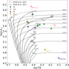 |
Fig. 7 Hertzsprung-Russell diagram for our sample. The non-rotating isochrones for different ages (≈[0–10] Myr) are overlaid as solid black lines, and the evolutionary tracks for stellar masses in the range ≈[10– 60] M⊙ with a rotational velocity of 50 km s−1 are shown as dashed black lines. The isochrones and evolutionary tracks were adopted from Brott et al. (2011). |
4 Results
We present below an overview of the results and compare them to other theoretical and empirical results that used the UV and optical or the optical range alone. The quality of our analysis is described for each star individually in Appendix F. Best fitting physical parameters are presented in Table A.1, including inferred evolutionary masses and ages from BONNSAI (Schneider et al. 2014) applied to Brott et al. (2011) rotating single-star evolutionary models for LMC metallicity.
4.1 Hertzsprung-Russell diagram
Fig. 7 shows the location of our targets on a Hertzsprung–Russell diagram (HRD). Our sample spans a range of temperatures log (Teff/K) ≈ 4.1–4.5, while luminosities cover a broad range of log (Lbol/L⊙) ≈ 4.50–6.10 (see Table A.1). The extremey luminous star is the hypergiant Sk −68◦ 135 with log (Lbol/L⊙) ≈ 6.1.
The majority of our sample exceeds log (Lbol/L⊙) ≈ 5.4, except for Sk −70◦ 16, which is a bright giant (II), and Sk −67◦ 195, which is a B8 Ib supergiant, according to Bestenlehner et al. (2025). Overall, the majority of the sample lies between the ZAMS and the terminal-age main sequence (TAMS), according to the evolutionary models of Brott et al. (2011), but several targets, assuming a single-star evolutionary scenario, are located beyond the TAMS and would therefore be identified as post-main-sequence stars.
Fig. 8 shows the location of our targets on the spectroscopic Hertzsprung-Russell diagram (sHRD) (Langer & Kudritzki 2014), where  and ℒ⊙ is calculated with solar values Teff = 5777 kK and log (g/cm s−1) = 4.44. The majority of our stars fall in the log ℒ /ℒ⊙ range of 4.0–4.3. We find that the hypergiants are the closest to the Eddington limit of log ℒ /ℒ ≈⊙ 4.6 (assuming a hydrogen mass fraction of 0.73). As expected, the low-luminosity supergiant Sk −67◦ 195 and the bright giant Sk −70◦ 16 are also farthest away from the Eddington limit, with log ℒ /ℒ⊙ equal to 3.68 and 3.82, respectively.
We also compare a calibration of the bolometric correction in the visual band BCV versus Teff to the calibration obtained by Lanz & Hubeny (2007) from TLUSTY non-LTE plane-parallel models of B stars. A simple fit to our dataset reveals
![Mathematical equation: \[B{C_{\rm{V}}}/{\rm{mag}} = 21.00 - 5.33{\rm{log}}\left( {{T_{{\rm{eff}}}}/{\rm{K}}} \right),\]](/articles/aa/full_html/2025/07/aa53799-25/aa53799-25-eq30.png) (6)
with a standard deviation of ≈0.1 mag, which support the results of Lanz & Hubeny (2007) for the LMC, who finds:
(6)
with a standard deviation of ≈0.1 mag, which support the results of Lanz & Hubeny (2007) for the LMC, who finds:
![Mathematical equation: \[B{C_{\rm{V}}}/{\rm{mag}} = 21.08 - 5.36\,{\rm{log}}\left( {{T_{{\rm{eff}}}}/{\rm{K}}} \right).\]](/articles/aa/full_html/2025/07/aa53799-25/aa53799-25-eq31.png)
As to be expected for a UV-bright sample, extinctions are relatively low with an average colour excess E(B − V) = 0.23± 0.06 mag, and an average total extinction in the V-band  mag. This agrees with the findings of Gordon et al. (2003).
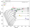 |
Fig. 8 Spectroscopic Hertzsprung-Russell diagram for our sample. The evolutionary tracks (solid black lines) and the isochrones (dashed black lines) are the same as in Fig. 7, which are taken from Brott et al. (2011). The Encoding of the luminosity classes is the same as in Fig. 7. |
4.2 Stellar masses
Evolutionary masses (Mevo) presented in Table A.1 are derived via a Bayesian inference method that is similar to BONNSAI (Schneider et al. 2014) with updated techniques (Bronner et al. in prep) applied to LMC tracks from Brott et al. (2011) with Lbol, Teff, log g, νrot sin i, and  as input parameters. Our sample spans a wide range range of
  to
to  . Table A.1 also includes stellar ages that range from
  to
to  .
.
In Table A.1, we present our values of the true surface effective gravity log (gc/cm s−2) = log (gmodel + νrot sin i2/R* ), where R* is obtained from Stefan–Boltzmann law. gc takes into account the centrifugal force due to stellar rotation (Herrero et al. 1992). Our values range from log gc ≈ 1.8 to 3.1 due to the stars possessing large radii (R* > 20 R ⊙ ), which is expected for a sample that consists of evolved OB stars.
We derive the spectroscopic masses (Mspec) from the gravities  . Therefore, we derive relative uncertainties of 20% −30%, which mainly depend on the uncertainties of log g, which is largely affected by quality of normalisation. To put this into perspective, a difference in the wings of the Balmer lines of 1% can potentially lead to a log g difference up to ≈ 0.1 dex. Such a difference leads to a relative uncertainty of ΔMspec ≈ 20%.
Spectroscopic masses are compared to evolutionary masses in Fig. 9. This shows that, for most of the stars, Mspec and Mevo are consistent within the uncertainties, similar to what Schneider et al. (2018) finds in a large sample of OB stars. For some of the stars (red circles in Fig. 9), the mass discrepancy that was established for Galactic O supergiants by Herrero et al. (1992), and later expanded to SMC O stars by Trundle et al. (2004) and further to Galactic B supergiants in Crowther et al. (2006) persists. We find that the spectroscopic masses for these stars are significantly lower than the masses produced by evolutionary models.
The Eddington parameter  presented in Table A.1 is derived using the evolutionary masses and it ranges from
  to
to  . We note that for the hypergiant Sk −68◦ 135 we obtain
  , which is unphysical, therefore we adopt the value corresponding to the lower limit of Γe = 0.89.
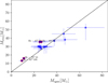 |
Fig. 9 Blue circles show the spectroscopically obtained mass from our analysis Mspec vs. the mass produced by BONNSAI (Schneider et al. 2014) applied to evolutionary tracks from Brott et al. (2011) Mevo. Red circles overlaid onto the blue points depict stars that have a significant discrepancy between their Mspec and Mevo. |
Wind parameters for our targets.
Slopes, a, and offsets, b, of the linear fits to the terminal wind velocity equation (Equation (7)) of this study and Hawcroft et al. (2024).
4.3 Wind properties
4.3.1 Terminal wind velocity ν∞
Measured wind velocities are presented in Table 4. In Fig. 10 we compare our ν ∞ − (Teff) to the empirical recipe of Hawcroft et al. (2024), adopting a simple linear fit of the form
![Mathematical equation: \[{v_\infty }\left[ {{\rm{km}}{{\rm{s}}^{ - 1}}} \right] = a{T_{{\rm{eff}}}}[{\rm{K}}] - b.\]](/articles/aa/full_html/2025/07/aa53799-25/aa53799-25-eq43.png) (7)
(7)
In Table 5, we present the parameters of the linear fit in Equation (7). We find that our ν ∞ -Teff relation agrees with the relation obtained by Hawcroft et al. (2024) within the uncertainties. We note that the two outliers are the hypergiants Sk −69◦ 279 and Sk −68◦ 135, which have abnormally low ν ∞ compared to stars of similar temperatures.
We also compare our results to numerical predictions of wind velocity from Vink & Sander (2021) and Krtička et al. (2024). The velocities calculated using the recipe provided in Vink & Sander (2021), which was obtained using a locally consistent Monte Carlo radiative transfer model (Müller & Vink 2008), agree with our measurements for stars located at the ‘cool’ side of the bi-stability jump predicted in Vink et al. (2001) (<25 kK), where as we find large discrepancies in the wind velocities of the objects that are located above the ‘hot’ edge of the bi-stability jump. As for the velocities calculated by the recipe presented in Krtička et al. (2024), we find that there is a discrepancy in the general trend, but just as in our results, there is a lack of a downward jump in the temperature range Teff ≈25–21 kK.
We also calculate the values of the escape velocity of each star (see Table 4) using the evolutionary mass obtained via BONNSAI as explained in Section 4.2. We discuss the implications of our findings later in Section 5.1.
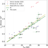 |
Fig. 10 v∞ vs. Teff for LMC supergiants. Green dots: results from this work, green line: linear fit of our results, yellow line: ν∞-Teff relation from Hawcroft et al. (2024), pink triangles: ν∞ calculated velocities from Vink & Sander (2021) recipe, violet diagonal cross: ν∞ calculated velocities from Krtička et al. (2021) recipe. |
4.3.2 Mass loss and clumping
Fig. 11 presents the spectral fits to Hα for all the stars in our sample. Aside from a few peculiar cases, our models well reproduce the overall shape and intensity of the emission feature in Hα as shown in. The results for the true mass-loss rates that are scaled to the transformed radius and volume-filling factor are presented in Table 4.
A good indicator of wind strength is the Eddington ratio (Γe = Lbol/Ledd), and it is expected that objects with higher Γe will have a greater mass-loss rate (Vink et al. 2011; Bestenlehner et al. 2014). In Fig. 12, a correlation between Γe and  is revealed.
We applied the spectral fits to a single XshootU observation, and we therefore present the Magellan/MIKE (Crowther 2024) Hα spectrum of Sk − 67◦ 78 in Fig. 13. Hα is significantly weaker in MIKE observations with respect to XshootU. This would lead to different  , β and fvol if we were to apply our fitting to MIKE data. Therefore, we include a factor of 2 in the uncertainties of the model mass-loss rates to take into account the possible variation in Hα and the additional error from having non-simultaneous UV and optical observations. This puts the uncertainty for the derived mass loss rates in the range Δ log
  dex.
dex.
For Sk −70◦ 16 and Sk − 67◦ 195 we adopt β = 1.0 due to Hα being fully in absorption. For the rest of our sample, we find that higher β = 2.0 ±0.6 are preferred to achieve a satisfactory fit for Hα. This is in agreement with Crowther et al. (2006) in which CMFGEN was used to model cool Galactic B supergiants, and they find that an average value of 2.0 for β is necessary to achieve a good fit. This is also in agreement with Haucke et al. (2018), in which they analysed Galactic B supergiants using FASTWIND and find that the suitable average value for β is also ≈ 2.0. We present our β values in Table 4.
Fig. 14 demonstrates the effect of varying β for Sk −68◦ 140. In the middle panel of Fig. 15, we present the line-formation region of Hα (blue solid line) for Sk −68◦ 140. The peak is at log (r/R* ) ≈0.2–0.4, which is well into the sonic regime of the atmosphere, and is averaged over a wide range of νwind (log (r/R* ) ≈ 0.1–0.8). From Equation (3) it is clear that increasing β lowers the acceleration of the wind. This leads to lower wind velocities at Hα line-formation region, where the wind has not yet reached it’s terminal velocity, resulting in higher densities at this region. This yields narrower red-shifted emission and blue-shifted absorption in Hα with less extended wings.
In Fig. 14, although the model with β = 2.5 (the blue solid line on Fig. 14) fits the blue shifted absorption better its emission is weaker than the observation, and the model with β = 2.0 (green solid line) fits the extended red wing of the emission but has an overly extended blue wing and is stronger than the observed emission. Therefore, we select the model with β = 2.2 (red solid line), which matches the observed emission and fits the overall morphology of the line.
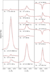 |
Fig. 11 Spectral fits to Hα for our sample of OB supergiants. Black line: observations, red line: model fit. |
 |
Fig. 12
|

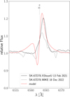 |
Fig. 13 Hα of Sk −67◦ 78 from MIKE observations (dashed black line) overlaid on Hα from XshootU (solid black line) with our best-fitting model (solid red line). |
4.4 Line-broadening parameters
In Table A.1, we include νrot sin i, the values of which are within reasonable agreement with the spectroscopic pipeline results from Bestenlehner et al. (2025). The values of νrot sin i we obtain for our stars are in the range ≈ 25–80 km s−1.
In Table 6, we compare our derived νrot sin i, which were obtained with the assumption of νmac = 20 km s−1, to the νrot sin i and νmac that were obtained by applying the IACOB-BROAD (Simón-Díaz & Herrero 2014) tool to a subsample of the stars with high-resolution MIKE data. IACOB-BROAD is a procedure based on a combined Fourier transform and goodness of fit approach that allows for the extraction of line-broadening parameters from a single snapshot of OB-type star spectra.
We used Si III λ4552 for all stars in the subsample except for the late supergiant Sk −67◦ 195, for which we use Si II λ6347. We find that our derived νrot sin i are in good agreement with those obtained from IACOB-BROAD. On the other hand, we systematically underestimate νmac by ≈ 10 km s−1. This implies that we could potentially be underestimating the CNO abundances in our sample, albeit this understimation is well within our adopted uncertainties of 0.3 dex.
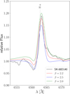 |
Fig. 14 Best-fitting model β = 2.2 (solid red line) vs. two other models with β = 2.5 (solid blue line) and β = 2.0 (solid green line) for Hα of Sk −68◦ 140 (solid black line). |
Comparison of our broadening parameters with those obtained via IACOB-BROAD (Simón-Díaz & Herrero 2014) applied to high-resolution MIKE data.
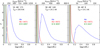 |
Fig. 15 Line formation region (ζ vs. log (r/R*)) of Hα (solid blue line), He I λ4471 (solid red line), and a line from the dominating nitrogen ion (solid green line) for Sk −66◦ 171 (Teff = 29.9 kK, left panel), Sk −68◦ 140 (Teff = 24.1 kK, middle panel), and Sk − 68◦ 8 (Teff = 14.1 kK, right panel). The grey shaded region indicates the photosphere. |
Best-fitting photospheric abundances ϵX.
4.5 He and CNO abundances
Table 7 presents the results for the chemical abundances of He and CNO elements. The analysis shows an overall boost in helium at the expense of hydrogen relative to the LMC baseline helium mass fraction of Y = 0.25 (Brott et al. 2011). This is to be expected for a sample of evolved stars. We would also expect nitrogen enrichment at the expense of oxygen and carbon, which get depleted due to CNO-cycle processing. Indeed, nitrogen abundances are significantly higher than the LMC baseline (Fig. 16), with a mean enhancement of 1 dex and a spread of 0.5 dex. We also note that our sample is mostly carbon and oxygen depleted with the exception of Sk − 71◦ 41 and Sk − 67◦ 2 where we find a 0.2 dex enhancement in oxygen.
Recalling Section 3.4.7, it is necessary to use lines of lower ionisation stages for B than for O stars. In panels d-l of Fig. 17, we use the best fitting models for Sk− 66◦ 171, Sk − 68◦ 140, and Sk− 68◦ 8 (left to right, respectively), which corresponds to temperatures of 29.9, 24.1, and 14.1 kK, respectively, to plot the radial ionisation structure of helium, nitrogen and iron. This shows that the atmosphere is dominated by lines of different ionisation levels depending on the temperature, which illustrates the reason behind fitting lines of lower ionisation stages with lower Teff.
In Fig. 15, we show the line formation regions of different lines versus radius νwind, and we can see that photospheric lines like He I λ4471 (red solid lines), N III λ4097, and N II λ4447 (green solid lines) form around νwind ≈ 10–15 km s−1, which coincides with the transition point between the subsonic and super-sonic regimes, connecting the photosphere to the inner region of the stellar winds. On the topmost panels of Fig. 17, the transition point is where the velocity jumps from 0 km s−1 to ≈ 15 km s−1.
Fig. 16 shows that the overall distribution of the observed nitrogen enhancement in our sample might be produced via evolutionary tracks that include rotational mixing (Brott et al. 2011). Extremely high initial rotational velocities disagree with what is observed for O stars and the findings of Ramírez-Agudelo et al. (2013), however, who obtained the rotational properties of a large sample of LMC O stars (216 stars) and concluded that the distribution of νrot sin i peaks at ≈ 80 km s−1. We found no clear positive correlation between rotation rates and nitrogen enhancement either, which is similar to the findings of Hunter et al. (2008).
In Fig. 18, we present the logarithm number ratios N/C and N/O of our sample (blue circles). Maeder et al. (2014) analytically obtains the upper and lower bounds (black dashed lines) from nuclear constraints (12C is turned immediately into 14N and the number of carbon atoms is constant throughout the CNO cycle) on the changes of N/C versus N/O ratios during the CNO cycle. We find that the majority of our stars are within those bounds. The exception are the stars Sk − 71◦ 41, Sk − 67◦ 5, Sk − 68◦ 52, Sk − 68◦ 140, which fall outside of the boundaries, but are within the uncertainties. In Fig. 18, we divide the stars into groups following the criteria introduced by Menon et al. (2024), who obtains the CNO abundances of 59 early-B supergiants in the LMC using FASTWIND. We find that only Sk − 71◦ 41 is part of Group 1, which is the group whose number ratios can be explained by a single star evolutionary scenario. Group 2, whose number ratios can be obtained via blue loop models, fast-rotating (νinit,rot = 220 km s−1) TAMS models, or merger models. The rest of the sample falls within Group 3, the number ratios of which can only be explained by merger scenarios.
Although it is expected for the combined mass fraction of CNO elements of any given star in our sample to stay constant throughout its evolution and to be similar to that of the LMC, we do find that, in some cases, the aggregate CNO mass fraction required to obtain a satisfactory fit to the designated CNO lines significantly diverges from the baseline CNO mass fraction of the LMC (ΣCNO/ΣCNOLMC in Table 7). The most extreme examples of this are Sk −71◦ 41 and Sk − 69◦ 279, with ratios of summed CNO mass fraction to LMC CNO mass fraction of ≈ 1.7 and 0.6, respectively, indicating that these objects have a respectively higher and lower cumulative CNO mass fraction. This likely arises from the sensitivity of abundances to other parameters, mainly Teff, log g. Fixing νmic, as explained in Section 3.4.4, could be a contributing factor to this discrepancy.
 |
Fig. 16 Nitrogen abundance (by number) vs. νrot sin i. The colour scheme corresponds to the value of log g, and the evolutionary tracks are computed for initial masses of 30 M⊙, 40 M⊙ and 50 M⊙ (red, brown, and orange solid lines respectively) for initial rotational velocities of 50, 110, 170, 220, 270 380 km s−1 (Brott et al. 2011), which we multiplied by a factor of π/4 to take into account the inclination of the rotation axis (Hunter et al. 2008). The black dashed line represents the LMC baseline nitrogen abundance. |
5 Discussion
In Section 5.1 we discuss the existence of the bi-stability jump in our sample. In Section 5.2 we compare our results to previous empirical studies. In Section 5.3, we compare our results to various numerical predictions. Finally, in Section 5.4 we explore the dependence of wind properties on metallicity.
5.1 Bi-stability jump
The main goal of this study is to explore the existence of the numerical mass-loss rate jump-like increase when going from the ‘hot’ regime to the ‘cool’ regime around Teff = 25 kK. We attempted to alleviate the degeneracy of mass loss and clumping that plagues the recombination line emission in Hα by using the appropriate unsaturated P Cygni lines in the UV, as mentioned above. Fig. 19 shows our derived wind efficiency parameter  versus Teff. The downward trend in the overall sample is clear. This agrees with Benaglia et al. (2007), who derive the mass-loss rates for a sample of Galactic OB stars from thermal radio emission and find a similar monotonic downward trend in wind efficiency with lower temperatures.
In Fig. 20, we compare the distribution of ν∞/νesc versus Teff to empirical predictions from Lamers et al. (1995) (MW) and Hawcroft et al. (2024) (LMC), plus the νesc–Teff prediction from Krtička et al. (2021) which does not assume a bi-stability jump, but rather a smooth transition from high to low ratios. Our sample show a smooth decline in ν ∞ /νesc with lower temperatures and lacks signs of a bi-stability jump around the proposed Teff ≈25–21 kK. Although the Krtička et al. (2021) recipe produces a smooth decrease in ν ∞ /νesc, our results do not match their prediction. The outliers are the hypergiants Sk − 68◦ 135 and Sk −69◦ 279, which have low ν ∞ /νesc. This is due to abnormally slow winds relative to other objects with similar temperatures.
The vertical error bars in Fig. 20 include the uncertainties of ν∞ and the νesc. With a simple linear fit we obtain the relation
![Mathematical equation: \[{v_\infty }/{v_{{\rm{esc\;}}}} = 4.1( \pm 0.8){\rm{log}}\left( {{T_{{\rm{eff\;}}}}/{\rm{K}}} \right) - 16.3( \pm 3.5).\]](/articles/aa/full_html/2025/07/aa53799-25/aa53799-25-eq64.png) (8)
(8)
5.2 Comparison to previous empirical studies
Due to differences in radiative transfer codes, in analysis methods and in observational datasets, and above all the lack of a clear unified method for calculating model and true uncertainties, we are not comparing like-for-like. The reason for the comparison is to check if the collection of those comparison studies produces an observable bi-stability jump.
Sander et al. (2024) concludes that an average maximum spread in Teff, log g, and log  obtained with different methods applied to ULYSSES/XshootU data is ΔTeff ≈ 3000 kK, Δ log (g/cm s−2) ≈ 0.2 and
  . While the analysis conducted by Sander et al. (2024) is very revealing of the discrepancies between the different radiative transfer codes and a great attempt at parametrising the spread that could be expected when comparing results obtained by these codes, the sample was limited to two LMC and one SMC O-type stars. Therefore, the spread of parameters obtained in that study is not significant from a statistical point of view.
We focus below on comparing Teff, log g, and log  . in Sections 5.2.1 and 5.2.2, when comparing the mass-loss rates, we do not adjust the values to the equivalent “smoothed wind” values (for fvol = 1).
Figs. 21–24 compare our derived values of Teff, log g,  , and log Lbol respectively, versus values derived in previous studies. We compile our derived Teff, log g, log
  , log Lbol, β, and fvol alongside the results of various previous empirical studies in Table D.1 in Appendix D.
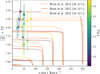 |
Fig. 17 Each column shows from left to right Sk − 66◦ 171 (Teff = 29.9 kK), Sk − 68◦ 140 (Teff = 24.1 kK), and Sk − 68◦ 8 (Teff = 14.1 kK). a, b, and c: Wind velocity as a function of radius in stellar radii units log (r/R *). d, e, and f : Ionisation structure (relative ionic density log (N(in+)/N(itot)) vs. log (r/R* )) of helium. g, h, i: Ionisation structure of nitrogen. j, k, and l: Ionisation structure of iron. i0 (orange), i+ (green), i2+ (red), i3+ (blue), i4+ (magenta), i5+ (black), and i6+ (grey) where i is the element. |
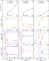 |
Fig. 18 log N/C vs. log N/O of our sample (grey triangles, blue circles, and red squares). The upper and lower boundaries (dashed black lines) are adopted from Maeder et al. (2014). The sample is divided into three groups depending on their N/C and N/O values, similar to Menon et al. (2024). |
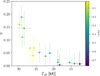 |
Fig. 19 Wind efficiency |

5.2.1 UV and optical studies
Evans et al. (2004) has two targets in common with the present study, also employed CMFGEN. Their Teff for the hypergiant Sk − 68◦ 135 is 1500 K lower than ours and a Teff for Sk − 68◦ 52 is 800 K higher than our estimate, whereas their log g is lower than ours by 0.15 dex and 0.12 dex respectively. They provide two mass-loss rates for each object, one with the assumption of a smooth wind, and the other with the assumption of a generic volume-filling factor of 0.1, and we compare our mass-loss rates to the latter and we find that their mass-loss rates are higher by 0.23 dex and 0.10 dex for Sk −68◦ 52 and Sk −68◦ 135, respectively. This can be attributed to the difference in photospheric parameters, the difference in β-law, which they assume is 2.75 and 3.50 respectively for Sk −68◦ 52 and Sk −68◦ 135, versus our β that we estimate at 2 and 2.3, and most significantly the large difference in the terminal wind velocity estimates, as we determine the wind velocities at 1140 km s−1 and 880 km s−1, versus their ν ∞ of 1400 km s−1 and 1350 km s−1 for Sk− 68◦ 52 and Sk− 68◦ 135, respectively, which they measure from the N III λ991 doublet in the FUV FUSE range. The luminosities obtained by Evans et al. (2004) are consistent within 0.1 dex of our luminosities.
We share Sk −71◦ 41 in common with Ramachandran et al. (2018), who analysed a large sample of OB stars in the LMC N206 superbubble using the Potsdam Wolf–Rayet (POWR) code (Gräfener et al. 2002; Hamann & Gräfener 2003; Sander et al. 2015). Their Teff is slightly higher than ours (see Table D.1), but we do find a large discrepancy in log g, where they estimate it to be ≈ 0.3 dex higher than ours. The source of this observed discrepancy is unclear but could be the due to the difference in datasets. The mass-loss rate obtained by them is consistent with our mass-loss rates, albeit slightly lower.
We have seven targets in common with Verhamme et al. (2024) and four targets with Brands et al. (2025), who conducted a UV+optical analysis for B supergiants and hot O supergiants, respectively, using the genetic algorithm KIWI-GA, which uses FASTWIND non-LTE radiative transfer models. These studies both used the same spectroscopic dataset as this study (ULLYSES/XShootU dataset). We find that our effective temperatures is systematically lower than those of Verhamme et al. (2024) and Brands et al. (2025) by 1000–4000 K (see Fig. 21). This could be attributed to the differences between CMFGEN and FASTWIND in the treatment of helium and silicon lines (Massey et al. 2013), and the different analysis methods (genetic algorithm versus manual by-eye fitting).
For the coolest star Sk −67◦ 195, Verhamme et al. (2024) obtained the temperature through the He I and Si II lines, whereas we obtain our temperature from fitting the He I and Mg II lines. FASTWIND suffferce from known convergence problems below 15 kK (Lorenzo et al. 2025), therefore CMFGEN is more reliable. The higher temperatures of Verhamme et al. (2024) and Brands et al. (2025) lead to higher log g in comparison to our work. We find that our effective surface gravities are 0.1–0.25 dex lower than theirs (see Fig. 22). The luminosities obtained by Verhamme et al. (2024) and Brands et al. (2025) are systematically higher than ours by ΔLbol = 0.02–0.12 dex, albeit they are consistent within the uncertainties. The sole outlier is Sk − 67◦ 5, for which the lumiosity derived by Brands et al. (2025) is lower than ours by approximately Δ log Lbol = 0.5 dex. This arises from adopting incorrect UBV photometry by Brands et al. (2025). The use of the correct photometry yields log  for Sk − 67◦ 5 (Brands et al. 2025, priv. comm.), which is in better agreement with our derived luminosity of log Lbol = 5.89. We do not notice any trend in the difference between our mass-loss rates and those obtained by Verhamme et al. (2024) and Brands et al. (2025) despite the different clumping parametrisation. We do note that mass-loss rates from Verhamme et al. (2024) and Brands et al. (2025) are consistent with our mass-loss rates within the uncertainties.
The advantages of our analysis methods compared to Verhamme et al. (2024) are the detailed treatment of line blanketing in the UV provided in CMFGEN (see Fig. 2), the robust velocity measurements from P Cygni profiles in the UV, and the employment of Mg II 4481 when measuring the temperature of the coolest B supergiants where Si III lines are no longer present. The main disadvantages of our method are the lack of robust calculations of statistical model errors. Unlike FASTWIND, the treatment of clumping in CMFGEN is limited to micro-clumping, which in some cases yields poor fits to the red emission in P Cygni profiles and requires unrealistically low volume-filling factors (or high clumping factors) to obtain good fits for the blue absorption. Muijres et al. (2011) describes how optically thin clumps increase the predicted mass-loss rates, while the optically thick clumps can display an opposite effect. This might have a differential effect on object at either side of the bi-stability jump. This effect was recently explored by de Burgos et al. (2024a) in a large sample of Galactic OB stars, and they report a lack of evidence for a bi-stability jump. We found no correlation between the mass-loss rate and the clumping parameters, which agrees with Verhamme et al. (2024) and Brands et al. (2025).
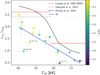 |
Fig. 20 Ratio (ν∞/νesc) as a function of temperature. The yellow dashed line is the relation presented in Krtička et al. (2021). The filled red lines represent the ratios from Lamers et al. (1995). The green filled line is the average relation for stars of spectral type earlier than B1 from Hawcroft et al. (2024). The colour gradient correlates to the value of Γe. |
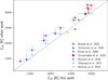 |
Fig. 21 Comparison of our obtained Teff to previous studies. We present on the x-axis our effective temperature for each star and the comparison Teff from previous analyses on the y-axis. Blue triangles: Comparison to values obtained by Verhamme et al. (2024), Red circles: Comparison to values obtained by Brands et al. (2025). Green filled crosses: Comparison to values obtained by Evans et al. (2004). Black square: Comparison to values obtained by Gvaramadze et al. (2018). Magenta diamond: Comparison to values obtained by Ramachandran et al. (2018). Cyan star: Our Teff to the effective temperatures from Urbaneja et al. (2017). Yellow hexagon: Comparison to values obtained by McEvoy et al. (2015). |
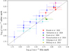 |
Fig. 22 Comparison of our obtained log g to previous studies. The symbols follow the same encoding as in Fig. 21. |
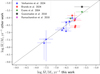 |
Fig. 23 Comparison of our derived |

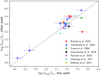 |
Fig. 24 Comparison of our derived log Lbol to previous studies. The symbols follow the same encoding as in Fig. 21. |
5.2.2 Optical-only studies
Sk − 68◦ 140 is in common with McEvoy et al. (2015), who obtained the atmospheric parameters and nitrogen abundances for a B supergiants in the LMC using TLUSTY and SYNSPEC codes (Hubeny & Lanz 1995). We find that our Teff and log g are slightly higher compared to theirs (500 K and 0.05 dex respectively), which falls well within our uncertainties. The model grids they use are plane-parallel and do not provide a measure of the mass-loss rate.
We share 4 targets in common with Urbaneja et al. (2017), which is a photometric and spectroscopic (optical only) study for LMC OB supergiants using FASTWIND. We find that, the effective temperatures are systematically larger than ours by 500–1500 K, whereas for log g we do not identify any systematic trend. Since Urbaneja et al. (2017) conducted their study to specifically explore the gravity–luminosity relation, mass-loss rates are not investigated. We find that our Teff and log g are consistent with theirs within the uncertainties. We calculate log Lbol from the total extinction values, bolometric corrections and apparent magnitudes provided in Urbaneja et al. (2017). We find that they are in agreement with our derived log Lbol within the uncertainties.
Gvaramadze et al. (2018) performed a detailed optical only spectroscopic analysis using CMFGEN for the hypergiant Sk − 69◦ 279. In comparison to our effective temperature and mass-loss rate, theirs are larger by 700 K and 0.4 dex, respectively. The difference in mass-loss is due to the difference in wind clumping, as they estimate fvol at 0.5 versus 0.1 in our analysis and β-law, which they fix at a value of 3, whereas we estimate a value of β = 2.7. The different observational data used in Gvaramadze et al. (2018) and the variable nature of this object, which resembles a dormant Luminous Blue Variable (LBV, Weis et al. 1997), could also be a contributing factor to this discrepancy. Gvaramadze et al. (2018) do not provide the effective surface gravity used in their models therefore we cannot compare our results.
Comparing our results to Bestenlehner et al. (2025), we find that there is a good agreement in the Teff and log g. The exception to this are the late-O hypergiants Sk −68◦ 135 and Sk −69◦ 279, where we find large differences in temperature and gravity. The discrepancy in Teff is likely due the weak He II λ4686 line, the region of which is clearly offset from the continuum (see Fig. I.3). Additionally, all Balmer lines used by the pipeline in Bestenlehner et al. (2025) present heavy wind contamination (fully or partially in emission), making log g hard to constrain. Subsequently, all the parameters obtained from fitting those lines are not reliable. Unlike other FASTWIND based studies, we do not notice a clear offset in Teff and log g. We find no major discrepancies in the luminosities. Despite the constant β = 1 and fvol = 0.1 in the grid that was used by the pipeline of Bestenlehner et al. (2025), their derived mass-loss rates are consistent with ours within the uncertainties.
5.3 Comparison to numerical mass-loss rate recipes
Here, we compare our derived mass-loss rates to those predicted by numerical recipes presented in Vink et al. (2001); Björklund et al. (2023); and Krtička et al. (2024). The mass-loss rate recipe produced by Vink et al. (2001) is based on predictions from unified Monte-Carlo models with consistency between radiative acceleration and mechanical acceleration in the over-all structure of the wind. The prediction of the bi-stability jump and the mass-loss rates around Teff = 25–21 kK in those simulations is due to the recombination of Fe IV into Fe III, which has significantly more spectral lines, resulting in a boost in line-driving. In the bottommost row of Fig. 17, it is clear the dominant iron ions at the connection point marking the photosphere in Sk −66◦ 171, Sk −68◦ 140, and Sk −68◦ 8 are Fe V, Fe IV, and Fe III, respectively. This means that the shift from Fe IV to Fe III is indeed reflected in our results, with Fe III providing the majority of line-driving (Petrov et al. 2016), but as we discuss later, this is not accompanied by an increase in empirical mass-loss rates. Petrov et al. (2016) explores another bi-stability jump at Teff ≈ 10–8 kK, which was discussed by Lamers et al. (1995) and Vink et al. (1999). This bi-stability jump is due to the change in ionisation balance between Fe III and Fe II, with Fe II becoming the source of most of the line acceleration.
An important element in the calculation routine is the ratio of terminal velocity to escape velocity (ν∞ /νesc). For this, we adopt the ν ∞ introduced in later study (Vink & Sander 2021). In Björklund et al. (2021, 2023), a locally self-consistent wind model FASTWIND that solves the radiative transfer equation in the co-moving frame is used. In this case, no sudden increase in the mass-loss rate is produced with decreasing Teff. In this recipe, the mass-loss rates decrease as a smooth function of stellar parameters. Finally, in Krtička et al. (2024) the mass-loss rates are derived using global stellar atmosphere code METUJE that was introduced in Krtička & Kubát (2017), which calculates the velocity stratification with the radiative acceleration. This recipe predicts a much more moderate increase in the mass-loss rates compared to what is predicted by Vink et al. (2001) in the regime bellow Teff = 20 kK.
Fig. 25 compares our derived mass-loss rates with the predicted mass-loss rates calculated by numerical recipes assuming Z/Z⊙ = 0.5. We notice that for stars with temperatures above 25 kK, the Vink et al. (2001) and Krtička et al. (2024) mass-loss rate predictions are relatively consistent with our derived mass-loss rates. For stars cooler that 25 kK our derived mass-loss rates are situated between Vink et al. (2001) and Krtička et al. (2024) favouring the latter in values and overall trend. Predictions from Björklund et al. (2023) have a similar trend to those from Krtička et al. (2024), but are consistently lower by ≈1 dex. The dip in the mass-loss rates in our results and in all predictions between Teff = 18–15 kK is due to the object Sk −70◦ 16 not being a B4 blue supergiant (Ib), but rather a lower luminosity bright giant.
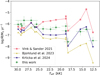 |
Fig. 25 Mass-loss rates as a function of Teff, comparing our derived |


Slopes, x, and offsets, log D0, of the linear fits to the modified wind momentum equation (Equation (9)) of this study, Mokiem et al. (2007), and Backs et al. (2024).
5.4 Metallicity effect
To explore the metallicity dependence of wind properties, we derive the modified wind momentum Dmom-Lbol relation  (Kudritzki et al. 1995; Kudritzki & Puls 2000), and we limit our fit to stars with log (Lbol/L⊙ ) > 5. For lower luminosity stars the mass-loss rates we obtain are less reliable and can be considered upper limits due to Hα being fully in absorption and due to the lack of reliable P Cygni profiles for wind velocity measurements. We fit our derived values using a Dmom-Lbol relation of the form
![Mathematical equation: \[\log D_{{\rm{mom}}}^{{\rm{LMC}}} = x\log \left( {{L_{{\rm{bol}}}}/{L_ \odot }} \right) + {\rm{log}}\,{D_0}.\]](/articles/aa/full_html/2025/07/aa53799-25/aa53799-25-eq77.png) (9)
(9)
Table 8 shows that our derived relation agrees well with the clumping-scaled relation derived by Mokiem et al. (2007) for LMC OB stars. Our Dmom–Lbol relation is consistent with the findings of Backs et al. (2024) within the uncertainties, however, they obtain a steeper relation from an LMC sample that consists mostly of O giants and bright giants, and incorporates results from Brands et al. (2025).
We also compare our results to those of Bernini-Peron et al. (2024), the latest detailed ULLYSES/XshootU spectroscopic analysis of an SMC B supergiant sample using CMFGEN. The main differences between our results and those of Bernini-Peron et al. (2024) is that, whereas we include late-O stars, their sample is composed from B stars exclusively. Their method differs from ours in that X-rays are included and νmic is a free parameter that is determined in their fitting procedure, which could lead to different temperature determination due to the change in opacity, which effects the depth of silicon lines. Higher νmic at larger radii in the wind could potentially also lead to underestimating ν∞.
In Fig. 26, we compare our derived Dmom-Lbol relation to that of Bernini-Peron et al. (2024). When fitting the results of their SMC sample we obtain:
![Mathematical equation: \[\log D_{{\rm{mom}}}^{{\rm{SMC}}} = 3.24( \pm 0.50){\rm{log}}\left( {{L_{{\rm{bol}}}}/{L_ \odot }} \right) + 9.8( \pm 2.8).\]](/articles/aa/full_html/2025/07/aa53799-25/aa53799-25-eq78.png)
There is a clear difference in the slope and vertical offset between the linear fit of the two samples, but unlike the findings of Mokiem et al. (2007), the two fits greatly vary, which is not something predicted by previous studies exploring the metallicity dependence of wind properties in the LMC and SMC for neither O nor B stars (e.g. Crowther et al. 2006; Mokiem et al. 2007; Backs et al. 2024). Excluding low luminosity objects, the sample of Bernini-Peron et al. (2024) spans a range of log Lbol/L⊙ ≈ 5.2–5.9, compared to the range of our sample log Lbol/L⊙ ≈ 5.5–6.1. The sample of Bernini-Peron et al. (2024) was also almost exclusively composed of Ia supergiants, and the authors inferred a selection bias to strong winds, whereas our sample contains supergiants from Ib to Ia+. These differences in the samples might be a major contributing factor to the difference in the dependence of the slope on the metallicity compared to previous studies.
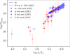 |
Fig. 26 Modified wind momentum-luminosity distribution of LMC (blue symbols) supergiants from this work and SMC (red symbols) supergiants from Bernini-Peron et al. (2024). Objects with log (Lbol/L⊙) < 5 are excluded from the linear fits for the LMC and SMC samples. The symbols for the SMC sample (red) follow the same encoding of the LMC sample (blue), where each luminosity class is given a unique symbol. |
6 Summary and conclusions
We have applied a quantitative analysis using CMFGEN models to LMC late-O and B supergiants, which we will also use in a future analysis of SMC (ULLYSES/XshootU) and Milky Way samples. We also compared our results to previous works, and we found that when the differences in the analysis methods and the quality of the data are taken into account, our parameters are mostly consistent with previously derived values within the expected systematic variance, which we discussed in Sander et al. (2024).
We found that our sample consists of evolved stars. The majority of the sample are main-sequence stars with a few post-main-sequence stars, according to the rotating single-star evolutionary models of Brott et al. (2011). Some of the stars in our sample appear to be evolved and in the post-main-sequence stage. The spectroscopic masses we derived are broadly consistent with the evolutionary masses obtained from BONNSAI (Schneider et al. 2014) within the uncertainties. Our results did not show the large mass discrepancy that was reported in previous studies (e.g., Herrero et al. 1992; Trundle et al. 2004; Crowther et al. 2006) (Schneider et al. 2018).
We obtained a velocity-temperature relation of
![Mathematical equation: \[{v_\infty }/{\rm{km}}\,{{\rm{s}}^{ - 1}} = 0.076( \pm 0.011){T_{{\rm{eff\;}}}}/{\rm{K}} - 884( \pm 260),\]](/articles/aa/full_html/2025/07/aa53799-25/aa53799-25-eq79.png) which agrees with the relation obtained by Hawcroft et al. (2024). We also derived a wind momentum-luminosity relation of
which agrees with the relation obtained by Hawcroft et al. (2024). We also derived a wind momentum-luminosity relation of
![Mathematical equation: \[{\rm{log}}\,D_{{\rm{mom}}}^{{\rm{LMC}}} = 1.39( \pm 0.54){\rm{log}}\left( {{L_{{\rm{bol}}}}/{L_ \odot }} \right) + 20.4( \pm 3.0),\]](/articles/aa/full_html/2025/07/aa53799-25/aa53799-25-eq80.png) which is very similar to the relation obtained for OB stars in the LMC by Mokiem et al. (2007).
which is very similar to the relation obtained for OB stars in the LMC by Mokiem et al. (2007).
We investigated the existence of the bi-stability jump, and we found a lack of observational evidence in our sample that would support this boost in line-driving, and hence, in mass loss and momentum, despite the shift from Fe IV to Fe III. This agrees with the analysis of Verhamme et al. (2024), who conducted an analysis of a ULLUSES/XShootU LMC sample. This also agrees with the results of de Burgos et al. (2024a), who found no increase in the mass-loss rates over the bi-stability region in a large sample of Galactic blue supergiants. Our findings also support the results of Bernini-Peron et al. (2024), who did not detect a bi-stability jump in their sample of SMC blue supergiants.
Our results showed a strong correlation between ν∞/νesc and Teff, and we obtained the relation
![Mathematical equation: \[{v_\infty }/{v_{{\rm{esc\;}}}} = 4.1( \pm 0.8){\rm{log}}\left( {{T_{{\rm{eff\;}}}}/{\rm{K}}} \right) - 16.3( \pm 3.5).\]](/articles/aa/full_html/2025/07/aa53799-25/aa53799-25-eq81.png)
We found no evidence of a sharp drop in ν ∞ /νesc, which might be attributed to the shift from the low-density and high-velocity wind regime to the high-density and low-velocity regime that are associated with the bi-stability jump (Pauldrach & Puls 1990; Lamers et al. 1995; Vink et al. 2001; Petrov et al. 2016).
By comparing our results to a similar CMFGEN-based analysis of SMC BSGs (Bernini-Peron et al. 2024), we found strong evidence of a Z-dependence of the wind momentum. This supports previous findings and predictions from line-driving wind theory. We did not establish metallicity-dependent mass loss or momentum recipes. We elected to produce these empirical recipes in a future paper, where we will conduct our own analysis of SMC and MW OB supergiants.
In future studies, we will include stars of the same spectral range and analysis methods to ensure that we make a meaningful comparison in different environments and that the results for each sample can be compared to the others without inherent differences in method. Our goal is to produce an empirical recipe for the mass-loss rates for blue supergiants that connects the mass-loss rates to other environmental (metallicity) and intrinsic (temperature, mass, and so on) parameters of the star. This can in turn be added as input for evolutionary models (Yoon et al. 2006) and population synthesis models (Leitherer et al. 1999) that currently rely on numerical mass-loss rate recipes such as the one proposed by Vink et al. (2001). An empirical mass-loss recipe like this would provide an important counterpart based on observations. Moreover, because the recipe would be produced by applying the same analysis methods to samples in different environments, the obtained Z-dependence would be more robust.
Data availability
The supplimentary online material can be found on Zenodo2. Appendix E includes comments on the excluded targets. Appendix F includes comments on diagnostic-line fits for all the targets in our sample. Additionally, SED fits, diagnosticline fits, and overall spectral fits can be found in Appendix G, Appendix H, and Appendix I, respectively.
Acknowledgements
T.A. would like to thank the Science and Technology Facilities Council (STFC) for financial support through the STFC scholarship ST/X508743/1. We would also like to thank Nidia Morrell for collecting and reducing MIKE data. JMB and PAC acknowledge financial support from the Science and Technology Facilities Council via research grant ST/V000853/1 (P.I. Vik Dhillon). DP acknowledges financial support from the FWO junior postdoctoral fellowship No. 1256225N. RK acknowledges financial support via the Heisenberg Research Grant funded by the Deutsche Forschungsgemein-schaft (DFG, German Research Foundation) under grant no. KU 2849/9, project no. 445783058. F.N. acknowledges support by PID2022-137779OB-C41 funded by MCIN/AEI/10.13039/501100011033 by “ERDF A way of making Europe”. This research has made use of the SIMBAD database, operated at CDS, Strasbourg, France, CMFGEN stellar atmosphere code developed by D. John Hillier, and BONNSAI software developed by Fabian Schneider. We would like to thank the referee for their critical and insightful input.
Appendix A Table of results
In Table A.1, Minit, Mevo, and ages of the stars are derived using an updated Bayesian inference method (Bronner et al. in prep) that is similar to BONNSAI (Schneider et al. 2014) applied to Brott et al. (2011) evolutioanry tracks. Γe is calculated using Mevo. Presented uncertainties for effective temperatures Teff are double the model uncertainty (see Section 3.4). In the uncertainties of centrifugal force-corrected surface gravity log gc, we take into account the model uncertainty of log g and the uncertainty of the projected rotational velocity ν rot sin i and the radius R*. The uncertainty in radial velocity ν rad measurements is dominated by the velocity resolution of the UBV part of the spectrum which is Δν ≈45 km s−1. The relative extinction RV (ΔRV ≈0.3 mag), colour excess E(B − V) (ΔE(B − V) ≈ 0.05 mag), absolute V-band magnitude MV, and bolometric correction BCV are produced from the SED fits that are shown in Appendix G.  is subject to uncertainties of
  which takes into account the uncertainties of Mspec and log Lbol.
Derived stellar parameters based on the best fitting CMFGEN model.
Appendix B νblack and νedge
In Table B.1 we present the measured νblack from each line for all our sample. Similarly, in Table B.2 we present the measured νedge.
νblack for the stars in our sample.
νedge for the stars in our sample.
Appendix C Atomic data
In Table C.1 we list the ions, number of important levels, super-levels, full levels, and transitions considered per ion, which constitutes the atomic model used in our CMFGEN model grid to synthesise the spectrum. The grid is split into two groups, with the boundary between the two set at ≈25 kK.
Ions and number of important levels (IL), super-levels (SL), full levels (FL), and transitions (T) considered per ion, which constitutes the atomic model (M) used by the code to synthesise the spectrum.
Appendix D Comparison to literature
We show Table D.1, in which we present our obtained values for Teff, log g, log  , fvol, and β in comparison to values presented in other previous studies. The volume-filling factor for studies that used the optically thick clumping is calculated from the equation introduced in Sander et al. (2024) following:
![Mathematical equation: \[{f_{{\rm{vol}}}} = \frac{{{{\left( {1 - {f_{{\rm{ic}}}}} \right)}^2}}}{{{f_{{\rm{cl}}}} - 2{f_{{\rm{ic}}}} + f_{{\rm{ic}}}^2}},\]](/articles/aa/full_html/2025/07/aa53799-25/aa53799-25-eq153.png) (D.1)
where fcl = ⟨ ρ2⟩ / ⟨ ρ 2⟩ describes the contrast between the density in the clump and the mean density, and fic describes the contrast between the clump density and the density of the inter-clump medium.
(D.1)
where fcl = ⟨ ρ2⟩ / ⟨ ρ 2⟩ describes the contrast between the density in the clump and the mean density, and fic describes the contrast between the clump density and the density of the inter-clump medium.
Comparison of derived parameters to previous studies.
References
- Alves, D. R. 2004, New A Rev., 48, 659 [Google Scholar]
- Anderson, L. S. 1985, ApJ, 298, 848 [NASA ADS] [CrossRef] [Google Scholar]
- Anderson, L. S. 1989, ApJ, 339, 558 [Google Scholar]
- Ardeberg, A., Brunet, J. P., Maurice, E., & Prevot, L. 1972, A&AS, 6, 249 [NASA ADS] [Google Scholar]
- Asplund, M., Grevesse, N., & Sauval, A. J. 2005, in Astronomical Society of the Pacific Conference Series, 336, Cosmic Abundances as Records of Stellar Evolution and Nucleosynthesis, eds. T. G. Barnes, III, & F. N. Bash, 25 [Google Scholar]
- Backs, F., Brands, S. A., de Koter, A., et al. 2024, A&A, 692, A88 [NASA ADS] [CrossRef] [EDP Sciences] [Google Scholar]
- Baum, E., Hamann, W. R., Koesterke, L., & Wessolowski, U. 1992, A&A, 266, 402 [NASA ADS] [Google Scholar]
- Beckman, J. E., & Crivellari, L. 1985, Science, 230, 835 [Google Scholar]
- Benaglia, P., Vink, J. S., Martí, J., et al. 2007, A&A, 467, 1265 [NASA ADS] [CrossRef] [EDP Sciences] [Google Scholar]
- Bernini-Peron, M., Marcolino, W. L. F., Sander, A. A. C., et al. 2023, A&A, 677, A50 [NASA ADS] [CrossRef] [EDP Sciences] [Google Scholar]
- Bernini-Peron, M., Sander, A. A. C., Ramachandran, V., et al. 2024, A&A, 692, A89 [NASA ADS] [CrossRef] [EDP Sciences] [Google Scholar]
- Bestenlehner, J. M., Gräfener, G., Vink, J. S., et al. 2014, A&A, 570, A38 [NASA ADS] [CrossRef] [EDP Sciences] [Google Scholar]
- Bestenlehner, J. M., Crowther, P. A., Caballero-Nieves, S. M., et al. 2020, MNRAS, 499, 1918 [Google Scholar]
- Bestenlehner, J. M., Enßlin, T., Bergemann, M., et al. 2024, MNRAS, 528, 6735 [CrossRef] [Google Scholar]
- Bestenlehner, J. M., Crowther, P. A., Hawcroft, C., et al. 2025, A&A, 695, A198 [NASA ADS] [CrossRef] [EDP Sciences] [Google Scholar]
- Björklund, R., Sundqvist, J. O., Puls, J., & Najarro, F. 2021, A&A, 648, A36 [EDP Sciences] [Google Scholar]
- Björklund, R., Sundqvist, J. O., Singh, S. M., Puls, J., & Najarro, F. 2023, A&A, 676, A109 [NASA ADS] [CrossRef] [EDP Sciences] [Google Scholar]
- Brands, S. A., de Koter, A., Bestenlehner, J. M., et al. 2022, A&A, 663, A36 [Google Scholar]
- Brands, S. A., Backs, F., de Koter, A., et al. 2025, A&A, 697, A54 [NASA ADS] [CrossRef] [EDP Sciences] [Google Scholar]
- Bresolin, F., Kudritzki, R.-P., Mendez, R. H., & Przybilla, N. 2001, ApJ, 548, L159 [NASA ADS] [CrossRef] [Google Scholar]
- Brott, I., de Mink, S. E., Cantiello, M., et al. 2011, A&A, 530, A115 [NASA ADS] [CrossRef] [EDP Sciences] [Google Scholar]
- Butler, K., & Giddings, J. 1985, Newsletter on Analysis of Astronomical Spectra No. 9, University of London [Google Scholar]
- Choudhury, S., Subramaniam, A., & Cole, A. A. 2016, MNRAS, 455, 1855 [NASA ADS] [CrossRef] [Google Scholar]
- Cioni, M. R., Clementini, G., Girardi, L., et al. 2011, The Messenger, 144, 25 [NASA ADS] [Google Scholar]
- Crowther, P. A. 2019, Galaxies, 7, 88 [Google Scholar]
- Crowther, P. A. 2024, in IAU Symposium, 361, eds. J. Mackey, J. S. Vink, & N. St-Louis, 15 [Google Scholar]
- Crowther, P. A., Hillier, D. J., Evans, C. J., et al. 2002, ApJ, 579, 774 [Google Scholar]
- Crowther, P. A., Lennon, D. J., & Walborn, N. R. 2006, A&A, 446, 279 [NASA ADS] [CrossRef] [EDP Sciences] [Google Scholar]
- Cutri, R. M., Skrutskie, M. F., van Dyk, S., et al. 2003, VizieR Online Data Cata- log: 2MASS All-Sky Catalog of Point Sources (Cutri+ 2003), VizieR On-line Data Catalog: II/246. Originally published in: University of Massachusetts and Infrared Processing and Analysis Center, (IPAC/California Institute of Technology) [Google Scholar]
- de Burgos, A., Simón-Díaz, S., Urbaneja, M. A., & Negueruela, I. 2023, A&A, 674, A212 [NASA ADS] [CrossRef] [EDP Sciences] [Google Scholar]
- de Burgos, A., Keszthelyi, Z., Simón-Díaz, S., & Urbaneja, M. A. 2024a, A&A, 687, L16 [NASA ADS] [CrossRef] [EDP Sciences] [Google Scholar]
- de Burgos, A., Simón-Díaz, S., Urbaneja, M. A., & Puls, J. 2024b, A&A, 687, A228 [NASA ADS] [CrossRef] [EDP Sciences] [Google Scholar]
- Debnath, D., Sundqvist, J. O., Moens, N., et al. 2024, A&A, 684, A177 [NASA ADS] [CrossRef] [EDP Sciences] [Google Scholar]
- Dessart, L., & Hillier, D. J. 2010, MNRAS, 405, 2141 [NASA ADS] [Google Scholar]
- Dopita, M. A., Seitenzahl, I. R., Sutherland, R. S., et al. 2019, AJ, 157, 50 [Google Scholar]
- Evans, C. J., Crowther, P. A., Fullerton, A. W., & Hillier, D. J. 2004, ApJ, 610, 1021 [NASA ADS] [CrossRef] [Google Scholar]
- Fitzpatrick, E. L., & Massa, D. 1990, ApJS, 72, 163 [NASA ADS] [CrossRef] [Google Scholar]
- Fouesneau, M. 2025, 10.5281/zenodo.14712174 [Google Scholar]
- Geen, S., Agrawal, P., Crowther, P. A., et al. 2023, PASP, 135, 021001 [NASA ADS] [CrossRef] [Google Scholar]
- Gordon, K. D., Clayton, G. C., Misselt, K. A., Landolt, A. U., & Wolff, M. J. 2003, ApJ, 594, 279 [NASA ADS] [CrossRef] [Google Scholar]
- Gräfener, G., Koesterke, L., & Hamann, W. R. 2002, A&A, 387, 244 [NASA ADS] [CrossRef] [EDP Sciences] [Google Scholar]
- Green, J. C., Froning, C. S., Osterman, S., et al. 2012, ApJ, 744, 60 [NASA ADS] [CrossRef] [Google Scholar]
- Gvaramadze, V. V., Kniazev, A. Y., Maryeva, O. V., & Berdnikov, L. N. 2018, MNRAS, 474, 1412 [NASA ADS] [CrossRef] [Google Scholar]
- Haiman, Z., & Loeb, A. 1997, ApJ, 483, 21 [NASA ADS] [CrossRef] [Google Scholar]
- Hamann, W. R., & Gräfener, G. 2003, A&A, 410, 993 [CrossRef] [EDP Sciences] [Google Scholar]
- Haucke, M., Cidale, L. S., Venero, R. O. J., et al. 2018, A&A, 614, A91 [NASA ADS] [CrossRef] [EDP Sciences] [Google Scholar]
- Hawcroft, C., Sana, H., Mahy, L., et al. 2024, A&A, 688, A105 [NASA ADS] [CrossRef] [EDP Sciences] [Google Scholar]
- Herrero, A., Kudritzki, R. P., Vilchez, J. M., et al. 1992, A&A, 261, 209 [NASA ADS] [Google Scholar]
- Herrero, A., Puls, J., & Najarro, F. 2002, A&A, 396, 949 [CrossRef] [EDP Sciences] [Google Scholar]
- Hillier, D. J. 1990, A&A, 231, 116 [NASA ADS] [Google Scholar]
- Hillier, D. J. 1996, in Liege International Astrophysical Colloquia, 33, eds. J. M. Vreux, A. Detal, D. Fraipont-Caro, E. Gosset, & G. Rauw, 509 [Google Scholar]
- Hillier, D. J. 1997, in IAU Symposium, 189, eds. T. R. Bedding, A. J. Booth, & J. Davis, 209 [Google Scholar]
- Hillier, D. J., & Miller, D. L. 1998, ApJ, 496, 407 [NASA ADS] [CrossRef] [Google Scholar]
- Hillier, D. J., & Miller, D. L. 1999, ApJ, 519, 354 [Google Scholar]
- Hillier, D. J., Lanz, T., Heap, S. R., et al. 2003, ApJ, 588, 1039 [Google Scholar]
- Hubeny, I., & Lanz, T. 1995, ApJ, 439, 875 [Google Scholar]
- Hunter, I., Dufton, P. L., Smartt, S. J., et al. 2007, A&A, 466, 277 [NASA ADS] [CrossRef] [EDP Sciences] [Google Scholar]
- Hunter, I., Brott, I., Lennon, D. J., et al. 2008, ApJ, 676, L29 [NASA ADS] [CrossRef] [Google Scholar]
- Korn, A. J., Nieva, M. F., Daflon, S., & Cunha, K. 2005, ApJ, 633, 899 [NASA ADS] [CrossRef] [Google Scholar]
- Krtička, J., & Kubát, J. 2017, A&A, 606, A31 [NASA ADS] [CrossRef] [EDP Sciences] [Google Scholar]
- Krtička, J., Kubát, J., & Krtičková, I. 2021, A&A, 647, A28 [NASA ADS] [CrossRef] [EDP Sciences] [Google Scholar]
- Krtička, J., Kubát, J., & Krtičková, I. 2024, A&A, 681, A29 [NASA ADS] [CrossRef] [EDP Sciences] [Google Scholar]
- Kudritzki, R.-P., & Puls, J. 2000, ARA&A, 38, 613 [Google Scholar]
- Kudritzki, R. P., Lennon, D. J., & Puls, J. 1995, in Science with the VLT, eds. J. R. Walsh & I. J. Danziger, 246 [Google Scholar]
- Kudritzki, R. P., Bresolin, F., & Przybilla, N. 2003, ApJ, 582, L83 [Google Scholar]
- Kudritzki, R.-P., Urbaneja, M. A., Bresolin, F., et al. 2008, ApJ, 681, 269 [NASA ADS] [CrossRef] [Google Scholar]
- Kudritzki, R.-P., Urbaneja, M. A., Bresolin, F., et al. 2024, ApJ, 977, 217 [Google Scholar]
- Kurucz, R. L. 1979, ApJS, 40, 1 [NASA ADS] [CrossRef] [Google Scholar]
- Lamers, H. J. G. L. M., Snow, T. P., & Lindholm, D. M. 1995, ApJ, 455, 269 [Google Scholar]
- Langer, N. 2012, Annu. Rev. Astron. Astrophys., 50, 107 [Google Scholar]
- Langer, N., & Kudritzki, R. P. 2014, A&A, 564, A52 [NASA ADS] [CrossRef] [EDP Sciences] [Google Scholar]
- Lanz, T., & Hubeny, I. 2007, ApJS, 169, 83 [CrossRef] [Google Scholar]
- Leitherer, C., Schaerer, D., Goldader, J. D., et al. 1999, ApJS, 123, 3 [Google Scholar]
- Lorenzo, M., Garcia, M., Castro, N., et al. 2025, MNRAS, 537, 1197 [Google Scholar]
- Maeder, A., Przybilla, N., Nieva, M.-F., et al. 2014, A&A, 565, A39 [NASA ADS] [CrossRef] [EDP Sciences] [Google Scholar]
- Marcolino, W. L. F., Bouret, J. C., Martins, F., et al. 2009, A&A, 498, 837 [NASA ADS] [CrossRef] [EDP Sciences] [Google Scholar]
- Markova, N., Puls, J., Scuderi, S., & Markov, H. 2005, A&A, 440, 1133 [NASA ADS] [CrossRef] [EDP Sciences] [Google Scholar]
- Martins, F. 2011, Bull. Soc. Roy. Sci. Liege, 80, 29 [Google Scholar]
- Martins, F., Mahy, L., Hillier, D. J., & Rauw, G. 2012, A&A, 538, A39 [NASA ADS] [CrossRef] [EDP Sciences] [Google Scholar]
- Massa, D., Prinja, R. K., & Oskinova, L. M. 2024, ApJ, 971, 166 [Google Scholar]
- Massey, P. 2002, ApJS, 141, 81 [NASA ADS] [CrossRef] [Google Scholar]
- Massey, P., Neugent, K. F., Hillier, D. J., & Puls, J. 2013, ApJ, 768, 6 [Google Scholar]
- McErlean, N. D., Lennon, D. J., & Dufton, P. L. 1998, A&A, 329, 613 [NASA ADS] [Google Scholar]
- McErlean, N. D., Lennon, D. J., & Dufton, P. L. 1999, A&A, 349, 553 [NASA ADS] [Google Scholar]
- McEvoy, C. M., Dufton, P. L., Evans, C. J., et al. 2015, A&A, 575, A70 [NASA ADS] [CrossRef] [EDP Sciences] [Google Scholar]
- Menon, A., Ercolino, A., Urbaneja, M. A., et al. 2024, ApJ, 963, L42 [NASA ADS] [CrossRef] [Google Scholar]
- Mokiem, M. R., de Koter, A., Vink, J. S., et al. 2007, A&A, 473, 603 [NASA ADS] [CrossRef] [EDP Sciences] [Google Scholar]
- Moos, H. W., Cash, W. C., Cowie, L. L., et al. 2000, ApJ, 538, L1 [NASA ADS] [CrossRef] [Google Scholar]
- Muijres, L. E., de Koter, A., Vink, J. S., et al. 2011, A&A, 526, A32 [NASA ADS] [CrossRef] [EDP Sciences] [Google Scholar]
- Müller, P. E., & Vink, J. S. 2008, A&A, 492, 493 [NASA ADS] [CrossRef] [EDP Sciences] [Google Scholar]
- Negueruela, I., Simón-Díaz, S., de Burgos, A., Casasbuenas, A., & Beck, P. G. 2024, A&A, 690, A176 [NASA ADS] [CrossRef] [EDP Sciences] [Google Scholar]
- Pauldrach, A. W. A., & Puls, J. 1990, A&A, 237, 409 [NASA ADS] [Google Scholar]
- Pauldrach, A. W. A., Kudritzki, R. P., Puls, J., Butler, K., & Hunsinger, J. 1994, A&A, 283, 525 [Google Scholar]
- Petrov, B., Vink, J. S., & Gräfener, G. 2016, MNRAS, 458, 1999 [NASA ADS] [CrossRef] [Google Scholar]
- Prinja, R. K., Barlow, M. J., & Howarth, I. D. 1990, ApJ, 361, 607 [NASA ADS] [CrossRef] [Google Scholar]
- Przybilla, N., Butler, K., Becker, S. R., & Kudritzki, R. P. 2006, A&A, 445, 1099 [NASA ADS] [CrossRef] [EDP Sciences] [Google Scholar]
- Przybilla, N., Nieva, M.-F., & Butler, K. 2008, ApJ, 688, L103 [CrossRef] [Google Scholar]
- Puebla, R. E., Hillier, D. J., Zsargó, J., Cohen, D. H., & Leutenegger, M. A. 2016, MNRAS, 456, 2907 [NASA ADS] [CrossRef] [Google Scholar]
- Puls, J., Kudritzki, R. P., Herrero, A., et al. 1996, A&A, 305, 171 [Google Scholar]
- Puls, J., Urbaneja, M. A., Venero, R., et al. 2005, A&A, 435, 669 [NASA ADS] [CrossRef] [EDP Sciences] [Google Scholar]
- Puls, J., Vink, J. S., & Najarro, F. 2008, A&A Rev., 16, 209 [Google Scholar]
- Ramachandran, V., Hamann, W. R., Hainich, R., et al. 2018, A&A, 615, A40 [NASA ADS] [CrossRef] [EDP Sciences] [Google Scholar]
- Ramírez-Agudelo, O. H., Simón-Díaz, S., Sana, H., et al. 2013, A&A, 560, A29 [NASA ADS] [CrossRef] [EDP Sciences] [Google Scholar]
- Repolust, T., Puls, J., & Herrero, A. 2004, A&A, 415, 349 [NASA ADS] [CrossRef] [EDP Sciences] [Google Scholar]
- Rivero González, J. G., Puls, J., & Najarro, F. 2011, A&A, 536, A58 [NASA ADS] [CrossRef] [EDP Sciences] [Google Scholar]
- Rivero González, J. G., Puls, J., Najarro, F., & Brott, I. 2012, A&A, 537, A79 [NASA ADS] [CrossRef] [EDP Sciences] [Google Scholar]
- Roman-Duval, J., Fischer, W. J., Fullerton, A. W., et al. 2025, arXiv e-prints, [arXiv:2504.05446] [Google Scholar]
- Sana, H., Tramper, F., Abdul-Masih, M., et al. 2024, A&A, 688, A104 [NASA ADS] [CrossRef] [EDP Sciences] [Google Scholar]
- Sander, A., Shenar, T., Hainich, R., et al. 2015, A&A, 577, A13 [NASA ADS] [CrossRef] [EDP Sciences] [Google Scholar]
- Sander, A. A. C., Bouret, J. C., Bernini-Peron, M., et al. 2024, A&A, 689, A30 [NASA ADS] [CrossRef] [EDP Sciences] [Google Scholar]
- Schmidt-Kaler, T., Gochermann, J., Oestreicher, M. O., et al. 1999, MNRAS, 306, 279 [NASA ADS] [CrossRef] [Google Scholar]
- Schmutz, W., Hamann, W. R., & Wessolowski, U. 1989, A&A, 210, 236 [Google Scholar]
- Schneider, F. R. N., Langer, N., de Koter, A., et al. 2014, A&A, 570, A66 [NASA ADS] [CrossRef] [EDP Sciences] [Google Scholar]
- Schneider, F. R. N., Ramírez-Agudelo, O. H., Tramper, F., et al. 2018, A&A, 618, A73 [NASA ADS] [CrossRef] [EDP Sciences] [Google Scholar]
- Searle, S. C., Prinja, R. K., Massa, D., & Ryans, R. 2008, A&A, 481, 777 [NASA ADS] [CrossRef] [EDP Sciences] [Google Scholar]
- Simón-Díaz, S. 2020, in Reviews in Frontiers of Modern Astrophysics; From Space Debris to Cosmology, 155 [Google Scholar]
- Simón-Díaz, S., & Herrero, A. 2014, A&A, 562, A135 [NASA ADS] [CrossRef] [EDP Sciences] [Google Scholar]
- Skrutskie, M. F., Cutri, R. M., Stiening, R., et al. 2006, AJ, 131, 1163 [NASA ADS] [CrossRef] [Google Scholar]
- Smartt, S. J. 2009, ARA&A, 47, 63 [NASA ADS] [CrossRef] [Google Scholar]
- Smith, N. 2014, ARA&A, 52, 487 [NASA ADS] [CrossRef] [Google Scholar]
- Smith, R. K., Brickhouse, N. S., Liedahl, D. A., & Raymond, J. C. 2001, ApJ, 556, L91 [Google Scholar]
- Sota, A., Maíz Apellániz, J., Walborn, N. R., et al. 2011, ApJS, 193, 24 [Google Scholar]
- Stanway, E. R., & Eldridge, J. J. 2018, MNRAS, 479, 75 [NASA ADS] [CrossRef] [Google Scholar]
- Trundle, C., & Lennon, D. J. 2005, A&A, 434, 677 [NASA ADS] [CrossRef] [EDP Sciences] [Google Scholar]
- Trundle, C., Lennon, D. J., Puls, J., & Dufton, P. L. 2004, A&A, 417, 217 [NASA ADS] [CrossRef] [EDP Sciences] [Google Scholar]
- Urbaneja, M. A., Herrero, A., Bresolin, F., et al. 2005a, ApJ, 622, 862 [Google Scholar]
- Urbaneja, M. A., Herrero, A., Kudritzki, R. P., et al. 2005b, ApJ, 635, 311 [NASA ADS] [CrossRef] [Google Scholar]
- Urbaneja, M. A., Kudritzki, R. P., Gieren, W., et al. 2017, AJ, 154, 102 [NASA ADS] [CrossRef] [Google Scholar]
- Verhamme, O., Sundqvist, J., de Koter, A., et al. 2024, A&A, 692, A91 [NASA ADS] [CrossRef] [EDP Sciences] [Google Scholar]
- Vernet, J., Dekker, H., D’Odorico, S., et al. 2011, A&A, 536, A105 [NASA ADS] [CrossRef] [EDP Sciences] [Google Scholar]
- Vink, J. S., & Sander, A. A. C. 2021, MNRAS, 504, 2051 [NASA ADS] [CrossRef] [Google Scholar]
- Vink, J. S., de Koter, A., & Lamers, H. J. G. L. M. 1999, A&A, 350, 181 [Google Scholar]
- Vink, J. S., de Koter, A., & Lamers, H. J. G. L. M. 2000, A&A, 362, 295 [Google Scholar]
- Vink, J. S., de Koter, A., & Lamers, H. J. G. L. M. 2001, A&A, 369, 574 [NASA ADS] [CrossRef] [EDP Sciences] [Google Scholar]
- Vink, J. S., Muijres, L. E., Anthonisse, B., et al. 2011, A&A, 531, A132 [NASA ADS] [CrossRef] [EDP Sciences] [Google Scholar]
- Vink, J. S., Mehner, A., Crowther, P. A., et al. 2023, A&A, 675, A154 [NASA ADS] [CrossRef] [EDP Sciences] [Google Scholar]
- Weis, K., Chu, Y. H., Duschl, W. J., & Bomans, D. J. 1997, A&A, 325, 1157 [NASA ADS] [Google Scholar]
- Weßmayer, D., Przybilla, N., & Butler, K. 2022, A&A, 668, A92 [NASA ADS] [CrossRef] [EDP Sciences] [Google Scholar]
- Weßmayer, D., Przybilla, N., Ebenbichler, A., Aschenbrenner, P., & Butler, K. 2023, A&A, 677, A175 [NASA ADS] [CrossRef] [EDP Sciences] [Google Scholar]
- Woodgate, B. E., Kimble, R. A., Bowers, C. W., et al. 1998, PASP, 110, 1183 [NASA ADS] [CrossRef] [Google Scholar]
- Yoon, S. C., Langer, N., & Norman, C. 2006, A&A, 460, 199 [NASA ADS] [CrossRef] [EDP Sciences] [Google Scholar]
The Si IV absorption line at λ = 4089 Å is actually a blend of Si IV and O II (de Burgos et al. 2024b). Considering models with extended O II atomic levels, we find that the O II component contributes ≈9%, 10%, 62% to the equivalent width of the combined line at T eff = 30, 25, 20 kK, respectively, with both lines being very weak in the low Teff case.
All Tables
Slopes, a, and offsets, b, of the linear fits to the terminal wind velocity equation (Equation (7)) of this study and Hawcroft et al. (2024).
Comparison of our broadening parameters with those obtained via IACOB-BROAD (Simón-Díaz & Herrero 2014) applied to high-resolution MIKE data.
Slopes, x, and offsets, log D0, of the linear fits to the modified wind momentum equation (Equation (9)) of this study, Mokiem et al. (2007), and Backs et al. (2024).
Ions and number of important levels (IL), super-levels (SL), full levels (FL), and transitions (T) considered per ion, which constitutes the atomic model (M) used by the code to synthesise the spectrum.
All Figures
|
Fig. 1 Normalised XshootU spectra (Sana et al. 2024, DR1) in the blue optical range of the sample with identifications for a subset of the optical lines. For illustration purposes, we added an arbitrary offset of 0.5 for each spectrum. The fits to the violet, yellow, and red spectra for all stars are presented in Appendix I. |
| In the text | |
|
Fig. 2 Normalised UV spectra in the range of the sample, with the line identification for the UV lines. For illustration purposes, an offset of one was added. The coloured lines show the observations. The black lines show the model fits for each of the respective stars. Stellar features are indicated in black line labels, whereas green line labels indicate interstellar features. The HST gap at ≈1300 in the spectra of Sk 69◦ 52, Sk 68◦ 8 is due to appending observations from COS G130M and COS G160M. The gap at 1600 Å is due to appending observations from COS G160M and COS G185M. Other UV fits are presented at Appendix I. |
| In the text | |
|
Fig. 3 Grey triangles show the model grid, purple squares show LMC targets with temperatures ≤ 40 kK (from the literature), and green points show LMC targets with temperatures ≥40 kK. The overlaid lines are isochrones taken from Brott et al. (2011). |
| In the text | |
|
Fig. 4 O I λλλ7772–7774–7775 and O II λ4254 lines of the B8 super-giant Sk − 67◦ 195 (black line). Red line: the preferred model the temperature of which (Teff = 12.5 kK) was obtained from fitting He I λ4471 and Mg II λ4481, and a comparison with higher Teff = 14.0 kK. |
| In the text | |
|
Fig. 5 Examples of the effect of varying Teff on the quality of the fit. The best-fitting model is shown with the solid red line. Comparison model: blue solid line (ΔTeff = 700 kK). Observed XShootU spectrum: black solid line. (a, b) Sk −71◦ 41 (O9.5 Ib). (c, d) Sk −68◦ 52 (B0 Ia). (e, f) Sk −67◦ 78 (B3 Ia). |
| In the text | |
|
Fig. 6 Examples of the effect of varying log g on the quality of the fit. The best-fitting model is shown with the solid red line. Comparison model: blue solid line. Observed XShootU spectrum: black solid line. a: Sk −66◦ 171 (O9 Ia) (Δ log g = 0.05). b: Sk −67◦ 5 (B0 Ib) (Δ log g = 0.1). |
| In the text | |
|
Fig. 7 Hertzsprung-Russell diagram for our sample. The non-rotating isochrones for different ages (≈[0–10] Myr) are overlaid as solid black lines, and the evolutionary tracks for stellar masses in the range ≈[10– 60] M⊙ with a rotational velocity of 50 km s−1 are shown as dashed black lines. The isochrones and evolutionary tracks were adopted from Brott et al. (2011). |
| In the text | |
|
Fig. 8 Spectroscopic Hertzsprung-Russell diagram for our sample. The evolutionary tracks (solid black lines) and the isochrones (dashed black lines) are the same as in Fig. 7, which are taken from Brott et al. (2011). The Encoding of the luminosity classes is the same as in Fig. 7. |
| In the text | |
|
Fig. 9 Blue circles show the spectroscopically obtained mass from our analysis Mspec vs. the mass produced by BONNSAI (Schneider et al. 2014) applied to evolutionary tracks from Brott et al. (2011) Mevo. Red circles overlaid onto the blue points depict stars that have a significant discrepancy between their Mspec and Mevo. |
| In the text | |
|
Fig. 10 v∞ vs. Teff for LMC supergiants. Green dots: results from this work, green line: linear fit of our results, yellow line: ν∞-Teff relation from Hawcroft et al. (2024), pink triangles: ν∞ calculated velocities from Vink & Sander (2021) recipe, violet diagonal cross: ν∞ calculated velocities from Krtička et al. (2021) recipe. |
| In the text | |
|
Fig. 11 Spectral fits to Hα for our sample of OB supergiants. Black line: observations, red line: model fit. |
| In the text | |
|
Fig. 12
|
| In the text | |
|
Fig. 13 Hα of Sk −67◦ 78 from MIKE observations (dashed black line) overlaid on Hα from XshootU (solid black line) with our best-fitting model (solid red line). |
| In the text | |
|
Fig. 14 Best-fitting model β = 2.2 (solid red line) vs. two other models with β = 2.5 (solid blue line) and β = 2.0 (solid green line) for Hα of Sk −68◦ 140 (solid black line). |
| In the text | |
|
Fig. 15 Line formation region (ζ vs. log (r/R*)) of Hα (solid blue line), He I λ4471 (solid red line), and a line from the dominating nitrogen ion (solid green line) for Sk −66◦ 171 (Teff = 29.9 kK, left panel), Sk −68◦ 140 (Teff = 24.1 kK, middle panel), and Sk − 68◦ 8 (Teff = 14.1 kK, right panel). The grey shaded region indicates the photosphere. |
| In the text | |
|
Fig. 16 Nitrogen abundance (by number) vs. νrot sin i. The colour scheme corresponds to the value of log g, and the evolutionary tracks are computed for initial masses of 30 M⊙, 40 M⊙ and 50 M⊙ (red, brown, and orange solid lines respectively) for initial rotational velocities of 50, 110, 170, 220, 270 380 km s−1 (Brott et al. 2011), which we multiplied by a factor of π/4 to take into account the inclination of the rotation axis (Hunter et al. 2008). The black dashed line represents the LMC baseline nitrogen abundance. |
| In the text | |
|
Fig. 17 Each column shows from left to right Sk − 66◦ 171 (Teff = 29.9 kK), Sk − 68◦ 140 (Teff = 24.1 kK), and Sk − 68◦ 8 (Teff = 14.1 kK). a, b, and c: Wind velocity as a function of radius in stellar radii units log (r/R *). d, e, and f : Ionisation structure (relative ionic density log (N(in+)/N(itot)) vs. log (r/R* )) of helium. g, h, i: Ionisation structure of nitrogen. j, k, and l: Ionisation structure of iron. i0 (orange), i+ (green), i2+ (red), i3+ (blue), i4+ (magenta), i5+ (black), and i6+ (grey) where i is the element. |
| In the text | |
|
Fig. 18 log N/C vs. log N/O of our sample (grey triangles, blue circles, and red squares). The upper and lower boundaries (dashed black lines) are adopted from Maeder et al. (2014). The sample is divided into three groups depending on their N/C and N/O values, similar to Menon et al. (2024). |
| In the text | |
|
Fig. 19 Wind efficiency |
| In the text | |
|
Fig. 20 Ratio (ν∞/νesc) as a function of temperature. The yellow dashed line is the relation presented in Krtička et al. (2021). The filled red lines represent the ratios from Lamers et al. (1995). The green filled line is the average relation for stars of spectral type earlier than B1 from Hawcroft et al. (2024). The colour gradient correlates to the value of Γe. |
| In the text | |
|
Fig. 21 Comparison of our obtained Teff to previous studies. We present on the x-axis our effective temperature for each star and the comparison Teff from previous analyses on the y-axis. Blue triangles: Comparison to values obtained by Verhamme et al. (2024), Red circles: Comparison to values obtained by Brands et al. (2025). Green filled crosses: Comparison to values obtained by Evans et al. (2004). Black square: Comparison to values obtained by Gvaramadze et al. (2018). Magenta diamond: Comparison to values obtained by Ramachandran et al. (2018). Cyan star: Our Teff to the effective temperatures from Urbaneja et al. (2017). Yellow hexagon: Comparison to values obtained by McEvoy et al. (2015). |
| In the text | |
|
Fig. 22 Comparison of our obtained log g to previous studies. The symbols follow the same encoding as in Fig. 21. |
| In the text | |
|
Fig. 23 Comparison of our derived |
| In the text | |
|
Fig. 24 Comparison of our derived log Lbol to previous studies. The symbols follow the same encoding as in Fig. 21. |
| In the text | |
|
Fig. 25 Mass-loss rates as a function of Teff, comparing our derived |
| In the text | |
|
Fig. 26 Modified wind momentum-luminosity distribution of LMC (blue symbols) supergiants from this work and SMC (red symbols) supergiants from Bernini-Peron et al. (2024). Objects with log (Lbol/L⊙) < 5 are excluded from the linear fits for the LMC and SMC samples. The symbols for the SMC sample (red) follow the same encoding of the LMC sample (blue), where each luminosity class is given a unique symbol. |
| In the text | |
Current usage metrics show cumulative count of Article Views (full-text article views including HTML views, PDF and ePub downloads, according to the available data) and Abstracts Views on Vision4Press platform.
Data correspond to usage on the plateform after 2015. The current usage metrics is available 48-96 hours after online publication and is updated daily on week days.
Initial download of the metrics may take a while.