| Issue |
A&A
Volume 698, June 2025
|
|
|---|---|---|
| Article Number | A142 | |
| Number of page(s) | 21 | |
| Section | Galactic structure, stellar clusters and populations | |
| DOI | https://doi.org/10.1051/0004-6361/202553840 | |
| Published online | 11 June 2025 | |
Tracing the W3/W4/W5 and Perseus complex dynamical evolution with star clusters
1
Department of Physics and Astronomy ‘Augusto Righi’, University of Bologna,
via Gobetti 93/2,
40129
Bologna,
Italy
2
INAF – Astrophysics and Space Science Observatory of Bologna,
via Gobetti 93/3,
40129
Bologna,
Italy
3
Department of Astronomy, Indiana University,
Swain West, 727 E. 3rd Street,
IN 47405
Bloomington,
USA
4
INAF – Osservatorio Astrofisico di Arcetri,
Largo Enrico Fermi 5,
50125
Florence,
Italy
★ Corresponding author: This email address is being protected from spambots. You need JavaScript enabled to view it.
Received:
21
January
2025
Accepted:
14
April
2025
Abstract
The Perseus complex offers an ideal testbed to study cluster formation and early evolution as it hosts two major hierarchical structures (namely LISCA I and LISCA II) and the W3/W4/W5 (W345) region characterized by recent star formation. The aim of this work was to provide a full characterization of the population of star clusters in the W345 region, in terms of their structural, photometric, and kinematic properties. The clusters were then used to probe the dynamical properties of the W345 region and, on a larger scale, to investigate the evolution of the Perseus complex. We used Gaia DR3 data to search for star clusters in the W345 region and characterize them in terms of their density structure, ellipticity, internal dynamical state, and ages. We also used young stellar object (YSO) catalogs from near-infrared surveys cross-matched with Gaia data to probe their kinematics in the region. We identified five stellar clusters belonging to the W345 complex. The three younger clusters are still partially embedded in the gas and show evidence of expansion, while the older clusters cleared the surrounding gas. We also found that YSOs trace the parent gas structure and possibly its kinematics. Thanks to the 6D information available for star clusters, we followed their orbital evolution to assess the formation conditions and evolution of the complex. When accounting for the Galactic potential, we find that the Perseus complex is not dispersing. The observed expansion might be a projection effect due to stars orbiting the Galaxy at different velocities. In addition, we find that the LISCA I and W345 systems formed some 20–30 Myr ago just a few hundred parsecs away, while LISCA II was originally ≃0.75–1 kpc apart. Finally, we also assessed the impact of spiral arm perturbations by constructing a tailored Galactic potential that matches the observed Galactic spiral arm structure. We find that spiral structures drag star clusters toward higher-density regions, possibly keeping clusters closer for longer than the unperturbed, axisymmetric case.
Key words: methods: data analysis / astrometry / stars: formation / stars: kinematics and dynamics / open clusters and associations: general / galaxies: star clusters: general
© The Authors 2025
 Open Access article, published by EDP Sciences, under the terms of the Creative Commons Attribution License (https://creativecommons.org/licenses/by/4.0), which permits unrestricted use, distribution, and reproduction in any medium, provided the original work is properly cited.
This article is published in open access under the Subscribe to Open model. This email address is being protected from spambots. You need JavaScript enabled to view it. to support open access publication.
1 Introduction
Clustered star formation has been an important mode of star formation since the early Universe. It is widely accepted that most stars in galaxies (up to 90% in our Galaxy) form in groups, and spend some time gravitationally bound with their siblings while still embedded in their progenitor molecular cloud (e.g., Lada & Lada 2003). The vast majority of such systems will be disrupted in their first few million years of existence, due to mechanisms possibly involving gas loss driven by stellar feedback (Kroupa et al. 2001; Baumgardt & Kroupa 2007; Moeckel & Bate 2010; Pelupessy & Portegies Zwart 2012; Pfalzner & Kaczmarek 2013; Brinkmann et al. 2017) or encounters with giant molecular clouds (GMCs, Gieles et al. 2006). Nonetheless, a fraction of these systems will survive the embedded phase and remain bound over longer timescales.
The process of clustered star formation thus has major implications in many fundamental astrophysical areas, including i) the role of stellar feedback and gas expulsion on the cluster disruption; ii) the contribution of cluster formation to large-scale structures in their host galaxies; iii) the onset of the cluster emerging properties and their evolution; iv) the formation and retention of gravitational wave sources (Di Carlo et al. 2019); and v) the formation of multiple populations (e.g., Bastian & Lardo 2018; Gratton et al. 2019).
Star clusters are expected to form within GMCs with possibly significantly different properties, likely linked to the early organization of the clouds and environmental factors (Lada & Lada 2003; Longmore et al. 2014). In particular, large GMC complexes are expected to produce a large number of star clusters born with a variety of energy distributions (Blaauw 1964) and potentially organized in hierarchical multi-scaled structures that can scale down to the formation of compact and bound clusters (Dalessandro et al. 2021; Della Croce et al. 2023). In general, the formation of young stellar clumps and clusters, along with the expansion and dispersal of young star systems may be related to complex dynamical interactions between clusters and sub-clusters during their formation process, and also to the rapid removal of gas due to massive star winds and more violent events like Wolf-Rayet outbursts or supernova explosions that can have an impact on scales of several tens of parsecs. Precise astrometric information and accurate line-of-sight (LOS) velocities from the Gaia satellite and large ground-based spectroscopic surveys have allowed the exploration of star kinematics in recently formed stellar complexes. In particular, several studies provided evidence of coherent motion and expansion in young star clusters, OB associations, and larger stellar complexes (e.g., Wright & Mamajek 2018; Kounkel et al. 2018; Damiani et al. 2019; Kuhn et al. 2019, 2020; Cantat-Gaudin et al. 2019; Lim et al. 2020, 2022; Swiggum et al. 2021; Das et al. 2023; Della Croce et al. 2024; Wright et al. 2024; Jadhav et al. 2024; Sánchez-Sanjuán et al. 2024).
In this context, here we focus on the W3/W4/W5 region (hereafter W345) of the Perseus complex. W345 is a well-studied region of recent star formation, containing two giant H II regions (W4 and W5), a massive molecular ridge with active star formation (W3), and several embedded star clusters (Carpenter 2000; Koenig et al. 2008; Román-Zúñiga et al. 2015; Jose et al. 2016; Sung et al. 2017). In addition, we previously identified two major cluster aggregates within the Perseus complex, namely LISCA I (Dalessandro et al. 2021) and LISCA II (Della Croce et al. 2023). These systems encompass several star clusters embedded in a more diffuse stellar halo sharing similar properties in terms of 3D position, 3D velocity, ages, and chemical abundances. Their structural and kinematical properties suggest they might form a more massive cluster by merging smaller systems. The LISCA systems and the W345 region lie within the Perseus complex: a large and massive complex located toward the Galactic anticenter (at about 2-3 kpc from the Sun) characterized by recent star formation and showing low dispersion in chemical element abundances (Fanelli et al. 2022a,b). In addition, the complex spatially coincides with a spiral arm structure (see, e.g., Reid et al. 2019; Drimmel et al. 2025).
This aim of this work is to carefully characterize the star cluster population of the W345 region, and to use the star clusters within the Perseus complex to trace its formation conditions and evolution. We start by defining the cluster population in the W345 region in Sect. 2, and in Sect. 3 we present their structural, photometric, and kinematic properties. In Sect. 4 we progressively zoom out, studying the young star population in the W345 region and their connection to star clusters. Finally, in Sect. 5 we investigate the star cluster population and evolution of the Perseus complex in a broader Galactic framework. We draw our conclusions in Sect. 6.
2 Identifying star clusters in the W345 region
To study the stellar population of the W345 complex we preliminary retrieved from the Gaia archive1 sources with Galactic coordinates ℓ ∊ [133.5°; 138.5°], and b ∊ [-0.3°; 2°]. The ranges are defined such that they enclose the W345 complex as traced by the gas distribution at NIR wavelengths (e.g., from the allWISE survey, Wright et al. 2010). We further selected sources with G magnitude brighter than 18 (i.e., phot_g_mean_mag < 18) and having parallax and proper motion (PM) measurements (i.e., astrometric_params_solved = 31). We did not apply any prior cut in parallax or PM to avoid possible selection biases in tracing the stellar content (and thus cluster population) of the complex. Instead, we performed data-driven selections as explained in the following (see also Della Croce et al. 2023).
We performed an unsupervised clustering analysis on the whole catalog using the HDBSCAN2 algorithm (McInnes et al. 2017) to identify overdensities in the five-dimensional space of Galactic coordinates (ℓ, b), PM (μα*, μdelta;), and parallax (ω). After several tests, we adopted as input parameters min_cluster_size = 50 and min_samples = 30. This combination of parameters allowed us to recover all the known star clusters (e.g., Cantat-Gaudin & Anders 2020; Castro-Ginard et al. 2022; Hunt & Reffert 2021, 2023) in the sky region under investigation. Twelve overdensities were thus identified as star cluster candidates in the region, but four of them were then flagged as false detections by the post-processing routine. We refer to Hunt & Reffert (2021) for the details of the postprocessing routine. Briefly, the nearest-neighbor distance among candidate members and field stars is used as a proxy for local density contrast. Only structures significantly denser than nearby Galactic field stars are considered as true stellar clusters. The eight clusters identified in our analysis are all known in literature (e.g., Cantat-Gaudin & Anders 2020; Hunt & Reffert 2023). Namely, they are IC 1848, IC 1805, Berkeley 65, UBC 420, SAI 24, Tombaugh 4, Stock 7, and NGC 1027. We note that one additional cluster (with a reported number of members greater than 50) is known in the region: UBC 1242 (Castro-Ginard et al. 2022; Hunt & Reffert 2023). Our analysis recovered the cluster but was later rejected as a false positive from the post-processing routine, probably due to the small density contrast with respect to the surrounding field stars.
We then studied the parallax and PM distributions for the eight clusters identified. The observed parallax and PM distributions were deconvolved using Gaussian modeling and properly accounting for errors and correlations between measurements, thereby obtaining their intrinsic distributions. In particular, for each star i we defined the covariance matrix (e.g., Sivia & Skilling 2006)
 (1)
(1)
where δμα*, δμδ, and δω are the individual errors, and ρab is the correlation coefficient among the a and b quantities. Using the Extreme Deconvolution package3 by Bovy et al. (2011), we obtained the best fit mean PM components (〈μα*〉, 〈μδ〉) and parallax (〈ω〉), along with the corresponding dispersions around the mean values, namely σμ*, σμδ, σω. We ran this analysis on likely cluster member stars adopting a membership threshold, as defined by the clustering algorithm, of 90%) and selecting stars with reliable astrometry (Lindegren et al. 2021b): ruwe < 1.4, δω/ω < 0.2, and astrometric_excess_noise smaller than the 95th percentile (applied only to stars with astrometric_excess_noise_sig > 2). We tested different membership thresholds (down to 70%), finding compatible results, within the errors.
Figure 1 shows the parallax and PM intrinsic distributions. Some clusters are grouped in both spaces, including the young clusters typically associated with the W345 complex, such as IC 1848, and IC 1805. Therefore, to identify the stars belonging to W345 in the Gaia catalog, we exploited the intrinsic distributions of those clusters showing similar (within 3σ) parallax and PMs. In particular, five out of eight clusters presented compatible distributions in both spaces: IC 1848, IC 1805, Berkeley 65, UBC 420, and SAI 24. We then defined the sources belonging to the W345 region by selecting stars with parallax and PM within 3σ from the mean value of any of the five clusters. For the parallax, this translates into sources with ω ∊ [0.341; 0.515] mas. In the PM space, sources within 0.87 mas yr−1 from (〈μα*〉, 〈μδ〉) = (−0.539; −0.364) mas yr−1 were selected. The PM reference point was obtained as the average of the five mean cluster motions. Such ranges are also depicted in Fig. 1. These data-driven selections in parallax and PM allowed us to adopt some physically motivated ranges for the region under investigation, avoiding any a priori selection. The final catalog counts 8869 sources.
In Table 1, we list the mean cluster properties. We find a good agreement (<2σ) with Hunt & Reffert (2023) for IC 1848, IC 1805, and Berkeley 65 and an excellent (<1σ) agreement with Cantat-Gaudin & Anders (2020) for UBC 420, which is not included in the “bona fide” cluster sample by Hunt & Reffert (2023).
Finally, Fig. 2 shows a 2D density map of the region. Clusters clearly appear as overdensities and are clustered in three main regions corresponding to W4 (e.g., Lim et al. 2020), W5-E (e.g., Karr & Martin 2003), and W5-W (e.g., Morgan et al. 2004). The W3 region is indeed deeply embedded in the gas and hardly probed by Gaia (see, e.g., Román-Zúñiga et al. 2015).
Mean properties of clusters in the W345 complex.
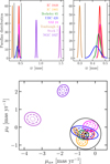 |
Fig. 1 Intrinsic (i.e., deconvolved) parallax (top panel), and PM (bottom panel) distributions for the eight clusters in the region defined by the preliminary Galactic coordinates ranges. The cluster names are reported in the top left panel. The black lines show the parallax and PM ranges adopted for selecting Gaia sources. The top right panel shows a narrower parallax range centered around the W345 star clusters to visualize the cluster parallax distributions better. Finally, in the bottom panel, the different contours represent the 1σ (dotted lines), 2σ (dashed lines), and 3σ (solid lines) regions for each cluster. The correlations among μα, and μδ are also visible. |
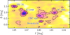 |
Fig. 2 Two-dimensional density map in Galactic coordinates of Gaia sources after the parallax and PM selections. The darker colors indicate denser regions. Iso-density contours at 0.5σ (solid), 1σ (dashed), and 1.5σ (dash-dotted) are shown in black. The cluster positions and names are marked. The density map was obtained through Gaussian kernel density estimate using the gaussian_kde function of the scipy Python package (Virtanen et al. 2020). |
3 Properties of star clusters in the W3/W4/W5 region
3.1 Structure
We constructed projected number counts density profiles for each cluster using stars with membership above 70%4. The density was obtained in spherically symmetric and evenly populated bins centered on the median cluster positions (see Table 1). In each radial bin, the density was computed as the average of the values obtained in four angular sectors and the standard deviation of these different measurements (summed in quadrature with Poissonian error) was adopted as the error. Figure 1 shows the cluster number density profiles obtained this way. We then fitted the observed density profiles with Plummer (1911) models (see Fig. 3). The best-fit models were obtained through a Markov chain Monte Carlo (MCMC) exploration of the parameter space, using the emcee5 Python package (Foreman-Mackey et al. 2013). In general, Plummer models reproduce the observed density profiles fairly well. The Plummer radii (RPlummer, inferred from the density profile fitting) and the 2D radii enclosing half of the members (R50, directly computed from the cluster member spatial distributions) agree in general within less than 1σ (see Fig. 3, and the values reported in Table 2).
We further characterized the morphological properties of each cluster by determining the axis ratio (q) and the position angle (PA) defined respectively as the minor-to-major axis ratio and the angle between the semi-major axis and the positive x direction. Following our previous work (Dalessandro et al. 2024), we iteratively diagonalized the shape tensor (Zemp et al. 2011) until a 10% precision was attained. Figure 1 presents the spatial distribution of cluster members with best-fit ellipses overplotted on false RGB images of the gas emission in the region. The possible link between elongation and internal kinematics is discussed in Sect. 3.3, while the values are reported in Table 2. Generally, all clusters in our analysis are pretty elongated, with the youngest clusters representing the most extreme cases.
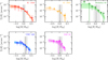 |
Fig. 3 Projected number density profiles for the five clusters analyzed in this study. Distances from the center were normalized to R50. Errors in each evenly populated bin were computed as the standard deviation of density measurements in different angular sectors (on the y-axis) and as the quantiles of the radial distribution within the bin (on the x-axis). The solid lines show the median Plummer model fit of the profile, whereas the shaded areas show the 68% (i.e., 1σ) confidence interval. Finally, the dashed black lines (the gray shaded areas) show the median Plummer scale radius (68% confidence interval) from the marginalized posterior distributions. |
Structural, photometric, and kinematic properties of clusters in the W345 complex.
3.2 Differential reddening and cluster ages
We constrained cluster ages by fitting the cumulative luminosity function in the differential reddening corrected G band as previously done in Della Croce et al. (2023). Differential reddening was computed using the same approach described in the same paper. Briefly, Gaia DR3 sources selected according to Sect. 2 were cross-matched with panSTARRS DR1 exploiting the matching tables provided by the Gaia Data Processing and Analysis Consortium. We thus retrieved g, r, i, z, and y-band photometry for the 98% of the stars selected in Gaia. We then used the color-color (G - r, i - z) diagram to assign star-by-star relative reddening values. In particular, for each star, we computed the distance along the reddening vector from the median colors of the closest 50 neighbors (to minimize fluctuations) and a reference point (see Della Croce et al. 2023, for further technical details). We used IC 1848 member stars as a reference, as previous studies (e.g., Cantat-Gaudin & Anders 2020; Hunt & Reffert 2023; Cavallo et al. 2024) roughly agree on the extinction value of this system, of about AV = 1.86 mag. On the contrary, either large discrepancies or much larger extinction values are reported for other clusters, such as Berkeley 65 orIC 1805. Figure 1 shows the resulting two-dimensional reddening map of the region: as expected, sparser areas are characterized by higher extinction values, suggesting that lower-density regions correspond to areas of significant photometric incompleteness. These under-sampled regions trace the spatial distribution of the W3, W4, and W5 GMCs (Koenig et al. 2008; Megeath et al. 2008).
Extinction coefficients also depend on the star effective temperature. This is particularly relevant for wide photometric bands (e.g., the Gaia G band) that span a large range of stellar temperatures (Jordi et al. 2010). We accounted for such an effect following Danielski et al. (2018) and using extinction temperature-dependent coefficients tailored to Gaia DR36. We note that such relations were calibrated for an effective temperature (Teff) range of 3500-10 000 K (Gaia Collaboration 2018), however for clusters as young as 5 Myr we sample stars as hot as Teff = 30 000 K. Nonetheless, we adopted such relations for all the stars, although they were extrapolated for the hottest stars in the sample. Figure 1 shows the differential reddening corrected color-magnitude diagrams along with the best-fit isochrones. As detailed in Della Croce et al. (2023), cluster ages were constrained using the cumulative luminosity function in the Gaia G band. The observed distributions were compared with synthetic simple stellar populations obtained from the PARSEC models (Bressan et al. 2012). The method was designed to account for statistical fluctuations in the main-sequence bright-end, possibly due to a combination of physical (e.g., short lifetimes) and instrumental (e.g., saturation) effects. To do so, we randomly picked the observed number of cluster member stars from the synthetic population one hundred times to quantify the probability of missing bright stars due to low numbers. Our analysis shows that the clusters in the W345 region are almost coeval with Berkeley 65 being the older one, with an age of  Myr. Table 2 reports the inferred ages, which are in good agreement with the literature estimates, confirming that IC 1805, IC 1848, and SAI 24 are the youngest clusters in the region (with an age of about 5 Myr). We note however, that we found a slightly older age for Berkeley 65 compared to previous estimates (see, e.g., Dias et al. 2021; Hunt & Reffert 2023; Cavallo et al. 2024, reporting an age in the range 10-17 Myr, although see also Cantat-Gaudin et al. 2020). Also, for UBC 420 we infer an age of
  Myr significantly younger than the reported age of ∼65 Myr by Cantat-Gaudin et al. (2020). The reason for the discrepancies may reside in the different member compilations. For example, no UBC 420 members with G < 9 mag are present in the catalog by Cantat-Gaudin et al. (2020), possibly leading to the inference of an older age. Nonetheless, our results confirm that the clusters in the W345 region are almost coeval. In this respect, a younger age for Berkeley 65 as suggested by previous studies would further strengthen the conclusion.
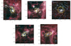 |
Fig. 4 On-sky spatial distribution of cluster members. For each cluster star, PM vectors are shown overplotted on the RGB image of the region from the allWISE survey. We mapped the W3 band in red, W2 in green, and W1 in blue. The W3 filter mainly traces small grain dust and polycyclic aromatic hydrocarbon emissions, whereas the W1 and W2 filters are dominated by young stars (Wright et al. 2010). The best-fit ellipses of the spatial distributions are shown in gold. |
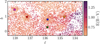 |
Fig. 5 Spatial distribution in Galactic coordinates of Gaia DR3 sources, selected according to Sect. 2. Each star is color-coded according to its reddening value. The crosses show the centers of the five stellar clusters analyzed in this work (SAI 24 in purple, IC 1848 in red, Berkeley 65 in green, UBC 420 in blue, and IC 1805 in yellow). |
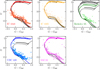 |
Fig. 6 Color-magnitude diagrams in the Gaia filters for cluster members. The best-fit isochrones from differential reddening-corrected G-band luminosity function fits are shown using the same color palette as cluster members. In black are multiple isochrones from literature works: Cantat-Gaudin et al. (2020); Dias et al. (2021); Hunt & Reffert (2023); Cavallo et al. (2024). |
3.3 Kinematics
In this section, we present the analysis of the internal dynamical properties of the five stellar clusters. Their kinematics can in principle give us insights into several physical processes: from the interplay between gas and stellar dynamics, the role of massive star feedback in both sweeping out the left-over gas and triggering star formation, up to cluster-cluster interactions.
In Fig. 4, we show the spatial distribution of likely member stars overplotted on an image of the region using allWISE photometry (Wright et al. 2010). Fig. 4 shows that some clusters in the sample, namely IC 1848, IC 1805, UBC 420, and SAI 24 are still partially embedded in the gas (at least in projection), whereas Berkeley 65 does not show any clear evidence of surrounding gas. This is consistent with the picture of it being older (see Fig. 6), and having completely removed its primordial gas. Fig. 4 also shows the projected velocity vectors for member stars: at least three clusters exhibit clear expansion features (IC 1848, IC 1805, and SAI 24); IC 1805 stands out for amplitude and coherence. Consistently, previous studies reported evidence for expansion for these systems (e.g., Lim et al. 2020). Several processes can cause clusters to expand, such as left-over gas removal and violent relaxation processes (Elmegreen 1983; Mathieu 1983; Kroupa et al. 2001; Goodwin & Bastian 2006; Pelupessy & Portegies Zwart 2012; Dinnbier & Kroupa 2020a,b; Dinnbier et al. 2022; Farias &Tan 2023; Della Croce et al. 2024), tidal forces from nearby gas clouds (Elmegreen & Hunter 2010; Kruijssen et al. 2011), and sub-cluster interactions and mergers (e.g., Wright et al. 2019, but see also Sánchez-Sanjuán et al. 2024 for an in-depth analysis of the effects of sub-structures on the expansion observed in star-forming complexes). In this context, Lim et al. (2020) studied the internal kinematics of IC 1805 and found that the cluster is composed of an isotropic core (defined as the region within the half-mass radius) and an external expanding halo. By investigating the distribution of individual radial velocities7, we found that while a fraction of stars is symmetrically distributed around zero within 0.7 R50 (about the half-mass radius reported by Lim et al. 2020), there is an excess of stars departing from the cluster center with increasing speed, hence driving the expansion signal also within R50 (see, e.g., Fig. 7). Furthermore, most cluster members are enclosed within the tidal radius (roughly corresponding to 2.25 R50 according to the estimate by Lim et al. 2020) and there is no significant evidence of extra-tidal features. This suggests that internal processes are likely responsible for the observed expansion rather than Galactic tidal forces (as already suggested by Lim et al. 2020).
Expansion can also shape the cluster distribution if stars depart faster in one of two orthogonal directions, a process usually referred to as asymmetric expansion (see, e.g., Wright et al. 2019). In Fig. 4 we show the ellipses describing the cluster shapes. The PA and q defining these ellipses were obtained as described in Sect. 3.1 (values are reported in Table 2). All clusters exhibit significant deviation from spherical symmetry and complex structures (as routinely found in many star-forming regions; see, e.g., Cartwright & Whitworth 2004; Gutermuth et al. 2008; Sánchez-Sanjuán et al. 2024). We thus studied the distribution of individual radial velocities (vR, i.e., the proper motion vector projected along the radial direction from the cluster center) as a function of elliptical radii  (where x′ and y′ are projected Cartesian coordinates rotated according to PA), or distance along the semi-major axis (a). In the case of expansion-driven elongations, we would expect tighter correlations between vR and Rell (or a) than with circular radii. However, we did not find significant differences for all the clusters investigated except possibly for IC 1848. This suggests that the cluster's internal kinematics does not drive the present-day cluster morphologies. In contrast, it is likely inherited either from processes that occurred earlier (possibly tidal interactions or mergers) or from the parent gas structure.
Finally, we delved into the expansion features shown by the clusters. In particular, we used the ratio of the mean radial velocity to radial velocity dispersion, 〈υR〉/σR, as defined in Della Croce et al. (2024, see Table 2 for the results). This integrated quantity provides a direct indication of the expansion (〈υR〉/σR > 0), contraction (〈υR〉/σR < 0), or equilibrium (〈υR〉/σR = 0) state of the system. Also, it allows meaningful comparison between different clusters as opposed to absolute quantities like (〈υR〉) (see Della Croce et al. 2024). For the five clusters included in this study, we also computed radial profiles of  , presented in Fig. 7, which give us a more complete picture of the cluster's internal kinematics. Radial trends are observed in IC 1848, IC 1805, and SAI 24, reaching values as high as
  (see Fig. 7) while distributions consistent with equilibrium are found in Berkeley 65, and UBC 420. There are a few more additional interesting points highlighted in Fig. 7: Berkeley 65 shows a flat
  profile centered around 0 over a large radial extension (>3R50). On the other hand, the external stars of UBC 420 are departing from the cluster bulk members. This is particularly evident in the north-east side of the cluster (see Fig. 4) possibly suggesting that these stars are currently being stripped from the cluster.
Finally, we present the expansion properties of clusters in the W345 complex within the larger picture of the expansion of young Galactic clusters (Della Croce et al. 2024). In Figure 1 we show  as a function of the cluster ages for all the systems studied in Della Croce et al. (2024) along with the five clusters analyzed in this paper. The W345 complex clusters perfectly fit in the general emerging picture in which young (.30 Myr) stellar systems are preferentially expanding, while older ones are roughly compatible with equilibrium configurations. We also note that except for IC 1848, IC 1805, and SAI 24, other clusters were not included in our previous study due to missing LOS velocity in Tarricq et al. (2021) catalog. Here we adopted the mean LOS velocity of −39 km s−1 (obtained from high-resolution spectra by Fanelli et al. 2022b). Nonetheless, we checked that perspective effect corrections (van Leeuwen 2009) are typically negligible (<1%) for these clusters.
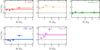 |
Fig. 7 Profiles of the mean radial velocity-to-radial velocity dispersion ratio. Cluster-centric distances were normalized to R50. The integrated values using all the cluster members are shown as horizontal lines (along with errors depicted as shaded areas). A black dashed line marks the zero expansion (contraction) level. |
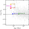 |
Fig. 8 Ratio of the radial mean velocity to velocity dispersion as a function of cluster age. The underlying data are from Della Croce et al. (2024). The different colors highlight the positions and results for the clusters analyzed in this work. |
4 Young stars in the W3/W4/W5 region: Their link with star clusters
On a larger scale, the Perseus complex is an extended region of recent star formation located toward the Galactic anti-center, which hosts several star clusters and associations. In particular, some of these clusters were found to be organized in larger hierarchical agglomerates that we named LISCA I (Dalessandro et al. 2021), and LISCA II (Della Croce et al. 2023). These are likely the fossils of the star formation within a large gas cloud a few tens of million years ago, and the possible progenitor of massive (a few  ) stellar systems forming hierarchically.
4.1 The YSO population
Young stellar objects (YSOs) trace the most recent star formation sites, typically younger than a few million years. They are thus used to trace star formation in giant molecular clouds and to constrain the role played by massive stars in either halting or promoting star formation (see Massey et al. 1995; Koenig et al. 2008; Megeath et al. 2008; Niwa et al. 2009; Morgan et al. 2009; Chauhan et al. 2011a,b, for a compilation of studies on the W345 complex). Many studies looked for YSOs in regions of recent star formation, primarily exploiting color-color selections for their identification (e.g., Allen et al. 2004; Whitney et al. 2004; Koenig et al. 2008; Snider et al. 2009; Cutri et al. 2013, 2021; Yadav et al. 2016; Jose et al. 2016; Panwar et al. 2017, 2019). YSOs indeed exhibit infra-red (IR) emission excess due to infalling, and illuminated material in their early stages and disk emission later on, historically referred to as Class I and Class II, respectively, and classified according to their near IR (NIR) spectral energy distribution slope (Adams et al. 1987; Whitney et al. 2003a,b). Also, young stars are prominent X-ray emitters due to magnetic reconnection flares at the stellar surface (see, e.g., Güdel & Telleschi 2007), hence X-ray observations could be used to complement infra-red catalogs of YSOs (Hofner et al. 2002; Feigelson & Townsley 2008; Rauw & Nazé 2016; Townsley et al. 2019).
Koenig et al. (2008) studied the star formation history of the W345 region, by using YSOs identified through the Spitzer space telescope. Furthermore, Panwar et al. (2017, 2019) characterized the low-mass YSO population around IC 1805 through a multiwavelength approach from the NIR to the X-rays. In particular, Panwar et al. (2019) supplemented the YSO catalog with WISE data. They used the YSO catalog by Cutri et al. (2013, 2021) from the allWISE program.
While these studies deeply characterized the YSO spatial distribution and its link with the gas, YSO kinematics in the region remains largely unexplored. We thus aim to study their kinematics in the context of the W345 complex. To do so, we cross-matched the catalogs by Koenig et al. (2008); Cutri et al. (2013, 2021); Panwar et al. (2019) with Gaia data. We selected Class I and Class II sources from Koenig et al. (2008), and nonextended, non-variable sources from Cutri et al. (2013, 2021), with confusion flags “000” and with photometric quality flags not worse than “B” in each band. The starting YSO catalog comprised 4096 sources almost half of which were from Koenig et al. (2008). The catalog was then cross-matched with Gaia DR3 sources selected in Sect. 2, obtaining a final catalog of 178 (about 4.4% of the starting one, out of which 129 had good astrometry according to Gaia quality flags, see Sect. 2) sources. We refer to this catalog as the Gaia YSO. In Fig. 9, we show the spatial distribution of Gaia YSOs with PM vectors shown as arrows. We note that: (i) YSOs are spatially concentrated either at the edges of the gas distribution or at young star cluster locations (e.g., SAI 24, IC 1848, IC 1805, see Sect. 3.2); (ii) YSOs trace the expansion observed in IC 1805, and IC 1848 (see Sect. 3.3); (iii) in the W5-E region (around  , see Karr & Martin 2003), YSOs are coherently moving northward. Given their position on the north side of the W5-E HII region, their motion may be inherited from the parent gas. This analysis further confirms that YSO kinematics is a powerful tool for tracing young cluster formation.
4.2 Bright-rimmed cloud ionizing sources
HII regions expanding in the surrounding gas might trigger star formation, forming the so-called bright-rimmed clouds (BRCs, Bertoldi 1989; Bertoldi & McKee 1990; Lefloch & Lazareff 1994, 1995). The bubble expansion drives shock in the surrounding medium possibly resulting in gravitationally unstable and triggering star formation (Thompson et al. 2004). The study of BRCs and whether they are star-forming or not (Sugitani et al. 1991; Sugitani & Ogura 1994) can thus provide valuable insights into the role of massive star feedback. In addition, identifying the feedback source is crucial to understanding how star formation proceeded.
In this section, we aim to tag candidate ionizing sources to known star clusters and investigate their kinematics within the cluster. First, we further confirm using Gaia DR3 parallaxes that the three regions (W3, W4, and W5) lie at the same distance from the Sun, hence their vicinity is not a projection effect, as already suggested by Xu et al. (2006); Hachisuka et al. (2006); Megeath et al. (2008).
We collected candidate ionizing sources from Morgan et al. (2004); Deharveng et al. (2012), and used the SIMBAD database to retrieve their Gaia DR3 source_id if present (see Table 3). This allowed us to look for each source in our cluster member catalogs. We found that at least one source for each region belonged to the central cluster. BD 60 507 is one of the candidate ionizing sources in W4, possibly triggering star formation in the BRCs 5, 7, 8, and 9 (Morgan et al. 2004). It belongs to the star cluster IC 1805 with a high membership probability (see Table 3). From Gaia data, we found that the star is close to the cluster center (about 0.5R50) and it is moving at about 0.1 mas yr−1 (i.e., roughly 0.95 km s−1 at 2 kpc) relative to the mean cluster motion. Moreover, the star has radial velocity spectrometer spectra, resulting in a fast rotator with vbroad = 180±48kms−1.
The candidate ionizing source for BRC 12 in the W5-West region is BD 60 586 (Morgan et al. 2004). This star was assigned to IC 1848 (with a membership of 65%). It is located at about 3.6R50 but it was not used in the IC 1848 kinematic characterization as it has ruwe = 2.74, suggesting that single-star track did not provide a good fit to the observed astrometry. Nonetheless, the generalized stellar parameterizer from photometry (GSP-Phot) provides  K.
K.
Concerning the W5-East region, BD 59 578 (also known as HD 18326) is widely referred to as the main ionizing source in the region (Chauhan et al. 2011a). According to our catalog, it belongs to SAI 24, being located ∼0.55R50 away from the cluster center, with a relative speed of 0.166 mas yr−1 (i.e., 1.57 km s−1 at 2 kpc). In addition, Deharveng et al. (2012) suggested V 1018 Cas as an additional ionizing source in W5-East for the observed pillars. The source belongs to SAI 24 although with lower membership, 72%. It lies at about 2R50 with a relative speed of 0.41 mas yr−1 (∼4 km s-1 at 2 kpc). According to the GSP-Phot, it has  K.
K.
Interestingly, none of the cross-matched sources was found to depart at a high relative speed from the cluster regardless of their cluster-centric distance and the expanding nature of the clusters (see Sect. 3.3). This further suggests that those massive stars constitute the core of the clusters. Figure 1 also shows the position of the candidate ionizing sources tagged to the different star clusters in the region.
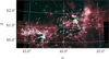 |
Fig. 9 Spatial distribution of the Gaia YSO sample, with PMs depicted with arrows. PMs were referred to the clusters mean motion in the regions (see Sect. 2). The background image is the composite RGB image of the W345 complex using data from the allWISE survey. The star symbols show the positions of the candidate ionizing sources in the region, color-coded according to the star cluster they are assigned to. |
Properties of the ionizing sources in the W345 complex.
5 The kinematics of the Perseus complex
Román-Zúñiga et al. (2019) studied the internal dynamics of the Perseus complex using a sample of young stars and Gaia DR2 data. The authors found a Hubble-like expansion flow in the region, with an estimated rate of 15 km s−1 kpc−1. As possible explanations, the authors suggested that the observed expansion could be due to supernova explosions in the region, interactions with the spiral arm, or the result of a large unbound stellar association that is expanding (Román-Zúñiga et al. 2019). Here we further investigate the dynamics of the complex using its star clusters. There are two main advantages in using star clusters: (i) the LOS component of the velocity is more widely accessible compared to individual stars, especially when dealing with luminous hot ones observed through Gaia RVS (Katz et al. 2023); (ii) average position and velocity are more precise and reliable as averaged among several member stars.
5.1 3D cluster positions and velocities
We constructed a catalog of star clusters in the Perseus complex by gathering the star clusters of the W345 region determined in this paper (see Sect. 3), in LISCA I (Dalessandro et al. 2021), and LISCA II (Della Croce et al. 2023). Cluster member catalogs were either presented in Sect. 2 (for W345) or in Dalessandro et al. (2021) and Della Croce et al. (2023). We obtained mean sky positions, PM components, and distances for all clusters directly from their members (defined by the membership threshold >90%). Also, we adopted homogeneous astrometric selections (see Sect. 2) and analysis. Cluster on-sky coordinates (α0, δ0) were obtained by averaging the positions of cluster members. To derive mean PM and distances for each cluster, we sampled the posterior distribution
 (2)
(2)
In Eq. (2),  is the array of mean quantities (with the distance in kiloparsecs), and
  is the array of observables for the i-th member star. In addition, the covariance matrix
  with Σi defined in Eq. (1) (to account for the non-negligible correlations in the Gaia astrometric solution), and
 (3)
(3)
where σμα*, σμδ, ρPM are the PM dispersions and correlation coefficients. Using Eq. (2) we can sample the joint posterior distribution in the mean PM components, velocity dispersions, correlation, and cluster distance. We note however that the distance term in Eq. (2) assumes cluster member stars to lie at the same distance (thereby neglecting the cluster depth) and parallax measurements for nearby stars to be independent (although see Vasiliev 2019b) as discussed by Cantat-Gaudin et al. (2018). Nonetheless, here we account for the correlation between PM and parallax as discussed in Sect. 2. We sample the joint posterior distribution (assuming uniform priors for the parameters) with an MCMC approach using the emcee package by Foreman-Mackey et al. (2013). Before sampling the posterior distribution, we accounted for the Gaia DR3 parallax bias following the prescription by Lindegren et al. (2021a).
Concerning the LOS velocity (vLOS) component, we merged multiple catalogs. We adopted the LOS velocity from the catalog with the largest number of member stars with LOS measurement between Tarricq et al. (2021) and Hunt & Reffert (2023), to have a more robust estimate of the mean LOS velocity. If a cluster had no measurements in these two catalogs, we searched for LOS velocity measurements in Tsantaki et al. (2022). The only exception to this general approach is the case of SAI 24. For this cluster, Tarricq et al. (2021) measured vLOS = +52 ± 22 km s−1 (using 8 stars), whereas Hunt & Reffert (2023) found vLOS = −48 ±5 km s−1 (using 7 stars). The two measurements are highly discrepant (3.7σ), possibly due to different membership compilations. However, the measurement from Hunt & Reffert (2023) is closer to the mean LOS velocity of the W345 complex (around −40 km s−1, Fanelli et al. 2022b) it belongs to. We thus adopted the value by Hunt & Reffert (2023). We note that SAI 24 is not included in the Tsantaki et al. (2022) catalog. Furthermore, the clusters UBC 420, Basel 10, and NGC 637 had no LOS velocity measurements in any catalog, whereas Berkeley 6 has a significantly lower vLOS in all the catalogs (has already pointed out in Della Croce et al. 2023).
Table 4 presents the six-dimensional phase-space information for the Perseus complex star clusters. The values reported for the distance and mean PM components represent the median value of the marginalized one-dimensional distribution, along with the 16th and 84th percentiles quoted as errors. Our results are generally consistent with those reported by the recent compilation of Hunt & Reffert (2023), although we find systematically lower values (.50 pc) for the cluster distances. We verified that the results presented in the following sections do not change if we adopted Hunt & Reffert (2023) catalog for the cluster data.
5.2 The projected kinematics
In this section, we present the projected kinematics of the Perseus complex as seen from a star cluster perspective. Figure 1 shows the absolute, on-sky velocities for the star clusters in the Perseus complex. LISCA II clusters are located in ℓ = 128-132 degree, LlScA I lies eastern at b < -2°, while in the region b = 0-2 degrees is W345. Román-Zúñiga et al. (2019) found a Hubble-like expansion pattern for the region using individual stars. The projected star cluster kinematics qualitatively fits into this picture: looking at the distribution of on-sky absolute PMs as a function of the projected distance we nicely recover the trend reported by Román-Zúñiga et al. (2019), finding a similar amplitude (see the top right panel in Fig. 10). However, considering the 3D cluster positions and velocities in the Galaxy, this large-scale motion is not observed. By a similar analysis, we found no net trend with the intrinsic distance (see the bottom right panel of Fig. 10). This may be because the Perseus complex spans more than 1 kpc along the LOS, hence when looking at the PM only we are projecting an almost 1.2 kpc-deep on a 10°-wide region (about 350 pc at 2 kpcs, see left panel of Fig. 10).
Given the available 6D data for clusters in the sample (Table 4), we thus investigated their dynamics in a broader, Galactic framework. Figure 1 presents the top-down view of the Galactic disk for the Perseus region. Star cluster positions and inplane velocities are shown color-coded according to the structure they belong to, along with the Perseus spiral-arm model from Reid et al. (2019). Interestingly, star clusters appear to be moving almost parallel to the arm. This, together with the Fig. 10 discussion, argues in favor of the Hubble-like expansion flow reported by Román-Zúñiga et al. (2019) likely being a projection effect arising from different orbital velocities at slightly different galactocentric distances. In this scenario, the Perseus complex kinematics is governed by the Galactic potential, possibly perturbed by the Perseus spiral arm, rather than internal dynamical processes.
Six-dimensional coordinates of the star clusters within the Perseus complex analyzed in this work.
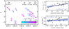 |
Fig. 10 Projected kinematic properties for the Perseus star clusters. Left panel: spatial distribution of the Perseus complex star clusters. The arrows show the PM vectors, converted in km s−1 according to the cluster distance (that is in turn shown using different marker sizes; see the coding in the top right corner of the plot). The color-coding shows vLOS . All data are reported in Table 4. The red diamond shows the claimed expansion origin according to the study of Román-Zúñiga et al. (2019). Right panels: distance-absolute velocity plots for the projected quantities (top) and 3D quantities (i.e., accounting for the position in the Galaxy and vLOS velocity, bottom), and assuming that the Sun lies at a distance of 8.178 kpc (GRAVITY Collaboration 2019) from the Galactic center, 20.8 pc above the disk (Bennett & Bovy 2021) and that it is orbiting in the Galaxy at (VX, VY, VZ) = (11.1, 248.5, 7.25) km s−1 (Schönrich et al. 2010; Reid & Brunthaler 2020). In the top panel, on-sky distances are from the expansion center suggested by Román-Zúñiga et al. (2019). The velocities and distances were converted to physical units assuming the distance ofIC 1805 (see Table 4). In the bottom panel, the 3D distances are relative to IC 1805. Errors are computed by the propagation of distance and vLOS errors (reported in Table 4). Both sub-panels show the linear regression obtained from the cluster data (in blue) and by Román-Zúñiga et al. (2019, in brown). The best-fit angular coefficient obtained in this work is also reported. Finally, the shaded areas represent the 68% credible interval, corresponding to 1σ if the distribution were Gaussian. |
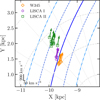 |
Fig. 11 XY projection of the star cluster galactocentric positions, while arrows show the VX, VY velocities (with velocity scale reported in the bottom left corner). Galactocentric coordinates were obtained by direct deprojection of the 6D coordinates listed in Table 4. Each cluster is color-coded according to the structure it belongs to: orange diamonds for W345, purple circles for LISCA I, and green squares for LISCA II . The blue lines show the Perseus spiral arm model (solid) by Reid et al. (2019), with once (dashed) and twice (dash-dotted) the arm width. The background grid is a heliocentric polar grid with the dashed gray lines showing distances from 1 to 4 kpc, and the dotted lines sampling the angular direction every 15 degrees. |
5.3 Orbits in an axisymmetric potential
We tested the hypothesis that the star clusters in the Perseus complex are not dispersing but rather orbiting in the Galaxy at slightly different galactocentric distances and speeds, by directly integrating their orbits. Starting from the 6D projected data (see Table 4), we obtained galactocentric coordinates and velocity components assuming that the Sun lies at a distance of 8.178 kpc (GRAVITY Collaboration 2019) from the Galactic center, 20.8 pc above the disk (Bennett & Bovy 2021) and that it is orbiting in the Galaxy at (VX, VY, VZ) = (11.1, 248.5, 7.25) km s−1 (Schönrich et al. 2010; Reid & Brunthaler 2020). Also, since we are measuring cluster mean positions (i.e., mean celestial coordinates and distances), and velocities (i.e., PMs and vLOS), literature catalogs provide errors in these quantities (Tarricq et al. 2021; Hunt & Reffert 2023, see Table 4). We thus accounted for distance and vLOS errors (typically the primary uncertainty sources) by sampling their distributions 500 times and obtaining galactocentric coordinates for all the extractions. Orbits were thus integrated in the axisymmetric McMillan (2017) potential using the Action-based Galaxy Modelling Architecture (AGAMA8) library (Vasiliev 2019a) for 200 Myr. In addition, to constrain the formation scenario and the initial size of the Perseus complex we performed a backward orbit integration by flipping the velocity vectors for each cluster. In the framework of the canonical set of angle-action coordinates (Binney & Tremaine 2008), this transformation allows us to follow the same orbit (as the action integrals are unchanged) but in the opposite direction along the angle space. Backward orbits were integrated for 50 Myr which is genearlly larger than the stellar ages in the region (Della Croce et al. 2023; Hunt & Reffert 2023; Cavallo et al. 2024). In Fig. 12, we show the topdown view of the Galactic plane with individual cluster orbits both forward and backward in time. Also, in Appendix A we present and discuss the time evolution of galactocentric coordinates for every cluster. There are a few interesting points to highlight from Fig. 12: i) LISCA I clusters move slightly outward in the Galactic plane, and toward LISCA II ; ii) two clusters, namely Berkeley 65 and NGC 869, depart the most from the other neighbor clusters (LISCA II and LISCA I clusters respectively). This is likely due to the difference in their vLOS to the other clusters (see Table 4); iii) going back in time in the cluster orbit reconstruction, LISCA I appears to converge toward the W345 complex.
Finally, we note that accounting for distance and vLOS errors is key in constraining the origin and evolution of star cluster systems. Although on Galactic scales the orbits are well constrained (see Fig. A.1) when looking at their distribution on cluster scales (or inter-cluster distance scales) errors on the initial conditions are far from negligible. This may also account for the apparent separation of LISCA II star clusters into two branches.
While individual star cluster orbits could give us insights into their evolution and origin, they may suffer of strong assumptions and shortcomings, particularly in the context of the Perseus complex. Star clusters in LISCA I and LISCA II are not isolated (Dalessandro et al. 2021; Della Croce et al. 2024). On the contrary, clusters are likely interacting with each other and they are also embedded in a more diffuse stellar halo. Therefore their present-day properties (mainly in terms of velocity distributions) may be strongly affected by their mutual interaction with other clusters. We thus decided to study the Persues complex at large using larger structures, such as the LISCA systems and clusters in the W345 region. We shall refer to these structures as cluster aggregates. Such an approach has multiple advantages. First, it allows us to trace the Perseus complex evolution on finer scales. Second, we are not considering star clusters as isolated entities, but rather as part of larger complexes (as suggested by previous studies, e.g., Dalessandro et al. 2021, and Della Croce et al. 2023). We note here, though, that despite the evidence of W345 complex star clusters being co-moving and co-spatial, treating them as a single aggregate does not imply any physical connection as for the LISCAs.
We obtained mean galactocentric positions and velocities for the cluster aggregates by averaging the individual cluster quantities. In particular, we followed Sivia & Skilling (2006) to estimate mean values and standard errors while taking into account heterogeneous errors. Finally, Fig. 12 (right panel) presents the cluster aggregate orbits projected on the XY plane. As anticipated, the use of cluster aggregates provides a clearer picture: LISCA I is currently in the process of drifting away from the W345 complex toward LISCA II, while LISCA II and W345 seems to evolve in parallel. Furthermore, in Fig. 13 we present the evolution of XYZ coordinates with time. Interestingly, the three structures evolve similarly in the plane for almost a full orbital period (of about 250-260 Myr) while experiencing different oscillation amplitude up and down the plane, with LISCA I showing the largest amplitude, up to 100 pc.
Finally, to quantitatively constrain the evolution and formation of the Perseus complex, we traced the 3D inter-aggregate distances with time (Fig. 14). At each time step, distances between the three cluster aggregates were computed for each orbit from the pool of initial conditions, and the median distance, along with the 16th and 84th percentiles, were obtained. We conclude that: (i) LISCA I is currently moving away from W345, reaching a distance of about 1.1 kpc in 100 Myr, before approaching it again; (ii) at the same time, LISCA I and LISCA II are getting closer, reaching minimum distance in about 30-40 Myr (iii) despite their appearance in the XY plane, LISCA II and W345 are approaching each other. In about 60 Myr they reach a distance of a few hundred parsecs, before slowly departing; (iv) concerning the backward integration, we can trace the formation condition of the Perseus complex. LISCA I and the W345 region were at their minimum distance about 25 Myr ago of just a few hundred parsecs, while LISCA II formed farther away, between 0.6-1 kpc; (v) we do not observe a Hubble-like expansion of the region as suggested by Román-Zúñiga et al. (2019). This highlights the importance of orbit integration (see, e.g., Fig. 14) and of using star clusters as tracers of the evolution of the complex.
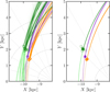 |
Fig. 12 XY projection for individual cluster orbits (left panel) and stellar cluster aggregates (right panel). Darker lines trace the orbits forward in time, whereas lighter lines trace backward. Thin lines show orbit integrations from multiple initial condition extractions, while thicker lines show median orbits. Present-day cluster positions are also marked: orange diamonds for W345, purple circles for LISCA I, and green squares for LISCA II clusters. |
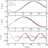 |
Fig. 13 Galactocentric coordinate time evolution for the star cluster aggregates. Darker lines are for integrations forward in time (i.e., t > 0), while lighter lines are for backward integrations (i.e., t < 0). The present-day positions are at t = 0. Initial conditions were sampled 500 times to account for errors in the mean distance and vLOS, and are shown by thin lines. The thicker solid lines are the median (of those multiple extractions) orbits. |
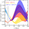 |
Fig. 14 Time evolution of all combinations of inter-aggregate 3D distances. Darker colors trace the forward integration (t > 0), while lighter colors are for the backward integration. Median distances are shown as solid lines, with shaded areas being the 16th (lower distance) and 84th (upper distance) percentiles of the 3D distance distributions from multiple initial condition extractions. The vertical gray area delimits the stellar age ranges, from 5 Myr (for W345 complex star clusters) to about 30 Myr for LISCA II (see Della Croce et al. 2023). |
5.4 Orbits in a spiral-perturbed potential
Figure 1 shows that Perseus star clusters lie on the spiral arm (Reid et al. 2019). Spiral structures (see Lin & Shu 1964; Shu 2016; Sellwood & Carlberg 1984, for different formation theories) are believed to play an important role in gathering gas, triggering star formation, and perturbing stellar orbits thanks to the locally deeper potential well (Baba et al. 2016; Tchernyshyov et al. 2018). In addition, Román-Zúñiga et al. (2019) suggested that the apparent expansion of the Perseus complex could be due to spiral arm interaction. We thus built a Galactic potential toy model in which we consider spiral arm perturbations to assess their effect on the cluster orbits.
We started from the spiral arm model provided by Reid et al. (2019). The authors modeled the spiral arm shape as
 (4)
(4)
where Rkink, and θkink are characteristic galactocentric radius (on the plane) and azimuth respectively, and ψ is the pitch angle. Also, they allowed the arm to abruptly change the pitch angle at θink and considered a distance-dependent arm width (see Fig. 11). Finally, Reid et al. (2019) concluded that the youngstar distribution is consistent with a five-arm model including the Scutum, the Sagittarius-Carina, the Local, the Perseus, and the Outer spiral arm. We thus used the potential formulation derived by Cox & Gómez (2002) for the density in Eq. (4), assuming each arm is a single spiral, and considered them as perturbations of the underlying axisymmetric potential (McMillan 2017). Such an approach has some assumptions and limitations that we discuss here. (i) The potential model (Cox & Gómez 2002) does not allow for a change in the pitch angle, we thus assumed the average value for ψ. In particular, for the Perseus arm, we assumed ψ = 9.5°; (ii) the amplitude of the density variations (f) with respect to the underlying potential is largely unconstrained by observations. This is a rather key parameter as increasing f enhances density perturbations. Levine et al. (2006) found that the density ratio of the arm to the inter-arm region using HI observations is about ∼3. Assuming that the stellar distribution presents the same ratio, we can translate it into f, finding that fHI = 0.53-0.66. However, this assumption is most likely wrong as the arm-to-inter-arm ratio for the gas is expected to be larger than the stellar one. The gas gathers in the overdensities (i.e., the spiral arm) thereby being converted into stars. On the other hand, stars formed in the arms can drift away populating the interarm region. Therefore, f HI represents an upper limit; (iii) recent studies found that spiral arm pattern speed decreases with galactocentric radius (Naoz & Shaviv 2007; Castro-Ginard et al. 2021). Our spiral arm model does not allow for different pattern speeds as orbits are integrated into the non-inertial, co-rotating frame. Since we are mainly interested in the role of the Perseus arm we decided to adopt the pattern speed Ωρ = 17.82 ± 2.98 km s−1 kpc−1 derived for the Perseus arm by Castro-Ginard et al. (2021) from the youngest open-cluster sample (that supposedly better traces the spiral structures in which they formed); (iv) our potential model does not include the bar which was shown to have a prominent impact on the Galactic stellar kinematics (e.g., Kawata et al. 2021 ; Drimmel et al. 2023). Orbits were integrated for at most 200 Myr, during which clusters orbit at about 10 kpc from the Galactic center. Hence the role of the bar could be treated as a second-order effect compared to the local spiral arm potential perturbations. We nevertheless present in Appendix B the orbits for a Galactic potential which includes the bar; (v) spiral arms unrealistically extend to the Galactic center, well beyond the data coverage (Reid et al. 2019). However, as discussed above, we are mainly interested in the local effects on the Perseus complex. Despite the aforementioned caveats, Fig. 15 shows the density map projected on the Galactic plane for the perturbed McMillan (2017) potential with f = 0.3. Qualitatively, the density potential model closely resembles the spiral arm structure presented by Reid et al. (2019, see the spiral structures in Fig. 15). We explored several f finding qualitatively similar results, and we present them in Appendix C.
Having built the Galactic potential, we computed the cluster aggregate orbits to study the evolution of the Perseus complex in the presence of spiral-arm perturbation. Figure 1 presents the evolution of galactocentric coordinates with time. We broadly found that the Perseus spiral arm pulls star clusters toward higher-density regions during their orbit. Since the star clusters in the Perseus complex are within the spiral arm, the stronger gravitational force may keep the star clusters closer for large times when compared to the axisymmetric case. Figure 1 shows the inter-aggregate distance evolution for the perturbed (f = 0.3) potential. Opposed to the axisymmetric case (Fig. 14), their relative distances oscillate between about 0.25-1 kpc for more than 200 Myr. However, star clusters may escape the spiral arm due to either differences in the orbital frequency and pattern speed or net relative inclination of the velocity vector to the arm pitch angle. In these cases, the Perseus spiral arm (or other nearby arms) drags the star clusters, profoundly changing the orbit. Such orbit perturbations are largely dependent on the value of f (see for instance Fig. C.3). Finally, integrating the orbits backward in time9 in the presence of spiral arm perturbations produces similar results with the interesting trend of decreasing the distance of LISCA II about 30 Myr ago with increasing f down to 500-750 pc (see Appendix C). This suggests that the Perseus complex could have been smaller in size if the spiral arms were more prominent when its major stellar associations formed.
We conclude that spiral arms play a role in shaping the cluster orbits and in the evolution of the Perseus complex. Also, different values of f do not qualitatively change the evolution on short timescales .100 Myr.
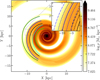 |
Fig. 15 Density map on the XY Galactic plane (i.e., computed at Z = 0) for a spiral perturbation with f = 0.3 (used as a reference model). The Sun is located at X = −8.178 kpc and Y = 0. The different colored lines present the different spiral arm models according to Reid et al. (2019): in dark green is the Outer arm, in blue Perseus arm, in black the Local arm, in cyan the Sagittarius-Carina arm, and in lime the Scutum arm. In the inset, we show a zoomed-in image of the Perseus region. |
6 Summary and conclusions
We studied the properties of the W345 region by using its cluster population and in the context of the more extended Perseus complex. We identified five clusters in the W345 region, namely IC 1805, IC 1848, Berkeley 65, UBC 420, and SAI 24, all previously known in the literature and all sharing similar 3D velocities and positions. All the clusters exhibit well-defined density structures, as shown by comparing the observed density profiles with theoretical models. They also present significant deviations from spherical symmetry. We found no evidence of a link between clusters' morphological properties and asymmetric expansion, thus suggesting the present-day spatial distribution is likely inherited from earlier processes or star formation. On the internal kinematics side, the three youngest clusters (IC 1805, IC 1848, and SAI 24) show prominent expansion, consistent with the picture that young star clusters are more likely to expand (Della Croce et al. 2024). A clear trend of  with the distance from the center is also observed within individual clusters, suggesting that expansion dominates cluster dynamics in the outskirts.
The W345 region was targeted by many studies that characterized the YSO population and spatial distribution. We complemented these studies by investigating the YSO kinematics within the region. YSOs were found to trace young star clusters' expansion and, most probably, the parent gas bulk motion. Finally, we characterized the candidate ionizing sources in H II regions and found that at least one for each H II region was classified as a high-probability (>65%) cluster member.
Finally, we further zoomed out to study the Perseus complex kinematics using its star clusters. Six-dimensional phase space data were obtained from the latest Gaia compilation coupled with large spectroscopic surveys (mainly for the LOS velocity component). Star clusters trace the expansion rate reported by Román-Zúñiga et al. (2019) when looking at on-sky coordinates. However, we found that such expansion is likely a projection effect due to different orbital velocities at slightly different galac-tocentric distances. Integrating the orbits of the three major structures in the complex (i.e., LISCA I, LISCA II, and W345), we traced their relative distance with time, and concluded that (i) LISCA I is drifting away from W345, reaching a distance of about 1.1 kpc in 100 Myr, before approaching it again; (ii) at the same time, LISCA I and LISCA II are getting closer, reaching their minimum relative distance in about 30-40 Myr; (iii) LISCA II and W345 are approaching each other: in about 60 Myr they will reach a distance of a few hundred parsecs, before slowly departing; and (iv) we did not observe the Hubble-like expansion of the region suggested by Román-Zúñiga et al. (2019). According to their reported rate, in 150 Myr the region should reach a size of about 5 kpc, inconsistent with their orbit in the Galaxy. In addition, backward orbit integration provides us with insights into the formation conditions of the Perseus complex: LISCA I and the W345 region were at their minimum distance about 25 Myr ago of just a few hundred parsecs, while LISCA II formed farther away, in the range 0.6-1 kpc.
We also tested the role of spiral-arm perturbations in the orbit evolution since the Perseus complex spatially coincides with the Perseus spiral arm (see, e.g., Reid et al. 2019). The spiral arm perturbs the cluster orbits by dragging them toward higher-density regions, thus possibly keeping clusters closer for longer times compared to the axisymmetric case. We found this result to be fairly robust on short timescales (.100 Myr) to varying density perturbation strength.
In summary, we presented a detailed characterization of the Perseus complex, starting from the clusters in the W345 region up to its kinematics on large scales by progressively zooming out. Particular attention was paid to complementing the numerous previous literature studies with kinematic data from Gaia DR3. We showed that the kinematics (supplemented by photometric and spectroscopic data) is key to understanding the formation and evolution of large stellar complexes from cluster scales to Galactic scales.
Acknowledgements
We thank the anonymous referee for their valuable comments that helped improve the paper. A.D.C. thanks L. Briganti, R. Pascale, L. Rosignoli, A. Mazzi, M. De Leo, and G. Ettorre for useful discussions. A.D.C. and E.D. would like to thank A. Sills and S. Kamann for their valuable feedback and comments on the Ph.D. thesis, of which this paper is a part. RGB images in this work were processed through the astronomical image processing tool SIRIL (Richard et al. 2024). We acknowledge financial support from the INAF Data Analysis Research Grant (ref. E. Dalessandro) of the 'Bando Astrofisica Fondamentale 2024'. This work uses data from the European Space Agency (ESA) space mission Gaia. Gaia data are being processed by the Gaia Data Processing and Analysis Consortium (DPAC). Funding for the DPAC is provided by national institutions, in particular, the institutions participating in the Gaia Multi-Lateral Agreement (MLA). This research or product makes use of public auxiliary data provided by ESA/Gaia/DPAC/CU5 and prepared by Carine Babusiaux. Data underlying this article will be shared upon reasonable request to the corresponding author.
Appendix A Perseus star cluster orbits in an axisymmetric potential
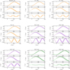 |
Fig. A.1 Temporal evolution of XYZ galactocentric coordinates for the 15 star clusters in the Perseus complex. Temporal evolution for 500 orbit integrations is shown with background thin lines. The initial conditions were extracted according to the distance and uLOS error distributions. The thicker foreground lines depict the median over multiple integrations. Cluster orbits are color-coded according to the larger cluster agglomerate to which they belong: orange for W345 complex, purple for LISCA I, and green for LISCA II. |
This section presents the individual cluster orbits integrated within the axisymmetric McMillan (2017) potential. The evolution of each cluster was followed for 200 Myr forward in time and 50 Myr backward. Figures A.1, and A.2 show the XYZ galactocentric coordinates as a function of time for all 15 clusters.
Appendix B Testing the impact of the Galactic bar
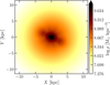 |
Fig. B.1 Density map on the XY Galactic plane (i.e., computed at Z = 0) for a Galactic potential which includes a tilted rotating bar. |
In this section, we present the impact of the Galactic bar on the cluster aggregate orbits. In particular, we constructed the bar potential as defined in Sormani et al. (2022). Briefly, the authors provided analytic formulae to match the N-body models by Portail et al. (2017). Such numerical models were in turn constrained to match the red clump stars density from a combination of infrared surveys, and the stellar kinematics in the bulge and the bar regions (Portail et al. 2017). The analytical model includes three components: an X-shaped, a long, and a short bar (Sormani et al. 2022). The model was implemented within the AGAMA library10 and considered as a perturbation of the McMillan (2017) potential (as done for the spiral arms, see Section 5.4). Figure B.1 shows the 3D density computed on the Galactic plane (Z = 0) constructed for such MW potential. The bar is roughly confined in the central 5 kpc, although resonances can strongly perturb orbits well outside that region. We assumed a tilt angle of −25° to the positive direction of the X axis.
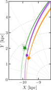 |
Fig. B.2 Orbits for the three stellar aggregates studied in this work on the Galactic plane. Orbits were computed within the potential model including the Galactic bar. |
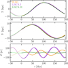 |
Fig. B.3 Galactocentric coordinate time evolution for the three stellar aggregates studied in this work. Orbits were computed within the potential model including the Galactic bar. The thin lines show the different integrations from the error distribution sampling of the initial conditions, while the thicker lines are the median position at any given time. |
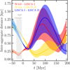 |
Fig. B.4 3D inter-cluster aggregate distance as a function of time. The orbits were computed in the Galactic potential which includes the bar. |
To quantitatively assess the impact of the Galactic bar, we then performed the same analysis as Section 5.3 but for the MW potential model with the bar. For the purposes of orbit integration, we assumed Ωp,bar = 37.5 km s-1 kpc-1 (Sormani et al. 2022). Figures B.2 and B.3 present the orbits in the MW model with the bar. In particular, Fig. B.2 shows the orbits projected onto the Galactic plane, while in Fig. B.3 the time evolution (both forward and backward) of the galactocentric coordinates are shown. Finally, the impact of the bar on the 3D relative distances of the aggregates is presented in Fig. B.4. As expected, the results are remarkably similar to those obtained in the purely axisymmetric case (see Fig. 14), thus confirming that the Galactic bar has a negligible effect on the Perseus cluster orbits compared to the local spiral arm structure.
Appendix C Exploring different f values
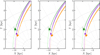 |
Fig. C.1 Stellar aggregate orbits on the Galactic plane for three values of f. From left to right f = 0.1, 0.3, 0.5, resulting in stronger density and potential perturbations. The different curves are orbits for different initial conditions extracted according to observed error distributions. The W345, LISCA I, and LISCA II orbits are in orange, purple, and green, respectively. Present-day positions are also shown with filled symbols. |
In this section, we show the cluster aggregates orbits for different non-axisymmetric potentials. Among the different integrations only f was changed exploring f = 0.1, 0.3, 0.5. Figure C.2 presents the XY projections of the aggregate orbits on the Galactic plane (f is increasing rightward). Similarly, Fig. C.2 presents the evolution with time of the XYZ coordinates for the three cluster aggregates. As could be seen, the stronger the density perturbation (i.e., increasing f) the more bend the orbits, which tend to follow the spiral structure. Finally, the implications of stronger spiral perturbations on the inter-aggregate distances are shown in Fig. C.3.
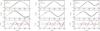 |
Fig. C.2 Temporal evolution of galactocentric coordinates for the three cluster aggregates integrated in different spirally perturbed potentials: from left to right f = 0.1, 0.3, 0.5. Darker colors show the forward integration for about 200 Myr, whereas lighter colors show the backward integration. The different colors depict different aggregates: the W345 complex in orange, LISCA I in purple, LISCA II in green. |
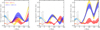 |
Fig. C.3 Inter-aggregate distance evolution for different spirally perturbed potentials. From left to right f = 0.1, 0.3, 0.5. We note the different scales on the y-axis. The gray shaded areas mark the cluster ages range, from 5-30 Myr. |
References
- Adams, F. C., Lada, C. J., & Shu, F. H. 1987, ApJ, 312, 788 [NASA ADS] [CrossRef] [Google Scholar]
- Allen, L. E., Calvet, N., D'Alessio, P., et al. 2004, ApJS, 154, 363 [Google Scholar]
- Baba, J., Morokuma-Matsui, K., Miyamoto, Y., Egusa, F., & Kuno, N. 2016, MNRAS, 460, 2472 [NASA ADS] [CrossRef] [Google Scholar]
- Bastian, N., & Lardo, C. 2018, ARA&A, 56, 83 [Google Scholar]
- Baumgardt, H., & Kroupa, P. 2007, MNRAS, 380, 1589 [NASA ADS] [CrossRef] [Google Scholar]
- Bennett, M., & Bovy, J. 2021, MNRAS, 503, 376 [NASA ADS] [CrossRef] [Google Scholar]
- Bertoldi, F. 1989, ApJ, 346, 735 [Google Scholar]
- Bertoldi, F., & McKee, C. F. 1990, ApJ, 354, 529 [NASA ADS] [CrossRef] [Google Scholar]
- Binney, J., & Tremaine, S. 2008, Galactic Dynamics, 2nd edn. [Google Scholar]
- Blaauw, A. 1964, ARA&A, 2, 213 [Google Scholar]
- Bovy, J., Hogg, D. W., & Roweis, S. T. 2011, Ann. Appl. Statist., 5, 1657 [Google Scholar]
- Bressan, A., Marigo, P., Girardi, L., et al. 2012, MNRAS, 427, 127 [NASA ADS] [CrossRef] [Google Scholar]
- Brinkmann, N., Banerjee, S., Motwani, B., & Kroupa, P. 2017, A&A, 600, A49 [NASA ADS] [CrossRef] [EDP Sciences] [Google Scholar]
- Cantat-Gaudin, T., & Anders, F. 2020, A&A, 633, A99 [NASA ADS] [CrossRef] [EDP Sciences] [Google Scholar]
- Cantat-Gaudin, T., Jordi, C., Vallenari, A., et al. 2018, A&A, 618, A93 [NASA ADS] [CrossRef] [EDP Sciences] [Google Scholar]
- Cantat-Gaudin, T., Jordi, C., Wright, N. J., et al. 2019, A&A, 626, A17 [NASA ADS] [CrossRef] [EDP Sciences] [Google Scholar]
- Cantat-Gaudin, T., Anders, F., Castro-Ginard, A., et al. 2020, A&A, 640, A1 [NASA ADS] [CrossRef] [EDP Sciences] [Google Scholar]
- Carpenter, J. M. 2000, AJ, 120, 3139 [Google Scholar]
- Cartwright, A., & Whitworth, A. P. 2004, MNRAS, 348, 589 [Google Scholar]
- Castro-Ginard, A., McMillan, P. J., Luri, X., et al. 2021, A&A, 652, A162 [NASA ADS] [CrossRef] [EDP Sciences] [Google Scholar]
- Castro-Ginard, A., Jordi, C., Luri, X., et al. 2022, A&A, 661, A118 [NASA ADS] [CrossRef] [EDP Sciences] [Google Scholar]
- Cavallo, L., Spina, L., Carraro, G., et al. 2024, AJ, 167, 12 [NASA ADS] [CrossRef] [Google Scholar]
- Chauhan, N., Ogura, K., Pandey, A. K., Samal, M. R., & Bhatt, B. C. 2011a, PASJ, 63, 795 [Google Scholar]
- Chauhan, N., Pandey, A. K., Ogura, K., et al. 2011b, MNRAS, 415, 1202 [NASA ADS] [CrossRef] [Google Scholar]
- Cox, D. P., & Gómez, G. C. 2002, ApJS, 142, 261 [NASA ADS] [CrossRef] [Google Scholar]
- Cutri, R. M., Wright, E. L., Conrow, T., et al. 2013, Explanatory Supplement to the AllWISE Data Release Products [Google Scholar]
- Cutri, R. M., Wright, E. L., Conrow, T., et al. 2021, VizieR On-line Data Catalog: II/328. Originally published in: IPAC/Caltech (2013) [Google Scholar]
- Dalessandro, E., Varri, A. L., Tiongco, M., et al. 2021, ApJ, 909, 90 [NASA ADS] [CrossRef] [Google Scholar]
- Dalessandro, E., Cadelano, M., Della Croce, A., et al. 2024, A&A, 691, A94 [NASA ADS] [CrossRef] [EDP Sciences] [Google Scholar]
- Damiani, F., Prisinzano, L., Micela, G., & Sciortino, S. 2019, A&A, 623, A25 [NASA ADS] [CrossRef] [EDP Sciences] [Google Scholar]
- Danielski, C., Babusiaux, C., Ruiz-Dern, L., Sartoretti, P., & Arenou, F. 2018, A&A, 614, A19 [NASA ADS] [CrossRef] [EDP Sciences] [Google Scholar]
- Das, S. R., Gupta, S., Prakash, P., Samal, M., & Jose, J. 2023, ApJ, 948, 7 [NASA ADS] [CrossRef] [Google Scholar]
- Deharveng, L., Zavagno, A., Anderson, L. D., et al. 2012, A&A, 546, A74 [NASA ADS] [CrossRef] [EDP Sciences] [Google Scholar]
- Della Croce, A., Dalessandro, E., Livernois, A., et al. 2023, A&A, 674, A93 [NASA ADS] [CrossRef] [EDP Sciences] [Google Scholar]
- Della Croce, A., Dalessandro, E., Livernois, A., & Vesperini, E. 2024, A&A, 683, A10 [NASA ADS] [CrossRef] [EDP Sciences] [Google Scholar]
- Di Carlo, U. N., Giacobbo, N., Mapelli, M., et al. 2019, MNRAS, 487, 2947 [NASA ADS] [CrossRef] [Google Scholar]
- Dias, W. S., Monteiro, H., Moitinho, A., et al. 2021, MNRAS, 504, 356 [NASA ADS] [CrossRef] [Google Scholar]
- Dinnbier, F., & Kroupa, P. 2020a, A&A, 640, A84 [EDP Sciences] [Google Scholar]
- Dinnbier, F., & Kroupa, P. 2020b, A&A, 640, A85 [EDP Sciences] [Google Scholar]
- Dinnbier, F., Kroupa, P., & Anderson, R. I. 2022, A&A, 660, A61 [NASA ADS] [CrossRef] [EDP Sciences] [Google Scholar]
- Drimmel, R., Khanna, S., D'Onghia, E., et al. 2023, A&A, 670, A10 [Google Scholar]
- Drimmel, R., Khanna, S., Poggio, E., & Skowron, D. M. 2025, A&A, in press, https://doi.org/10.1051/0004-6361/202451100 [Google Scholar]
- Elmegreen, B. G. 1983, MNRAS, 203, 1011 [NASA ADS] [CrossRef] [Google Scholar]
- Elmegreen, B. G., & Hunter, D. A. 2010, ApJ, 712, 604 [NASA ADS] [CrossRef] [Google Scholar]
- Fanelli, C., Origlia, L., Mucciarelli, A., et al. 2022a, ApJ, 931, 61 [Google Scholar]
- Fanelli, C., Origlia, L., Oliva, E., et al. 2022b, A&A, 660, A7 [NASA ADS] [CrossRef] [EDP Sciences] [Google Scholar]
- Farias, J. P., & Tan, J. C. 2023, MNRAS, 523, 2083 [NASA ADS] [CrossRef] [Google Scholar]
- Feigelson, E. D., & Townsley, L. K. 2008, ApJ, 673, 354 [Google Scholar]
- Foreman-Mackey, D., Hogg, D. W., Lang, D., & Goodman, J. 2013, PASP, 125, 306 [Google Scholar]
- Gaia Collaboration (Babusiaux, C., et al.) 2018, A&A, 616, A10 [NASA ADS] [CrossRef] [EDP Sciences] [Google Scholar]
- Gieles, M., Portegies Zwart, S. F., Baumgardt, H., et al. 2006, MNRAS, 371, 793 [Google Scholar]
- Goodwin, S. P., & Bastian, N. 2006, MNRAS, 373, 752 [Google Scholar]
- Gratton, R., Bragaglia, A., Carretta, E., et al. 2019, A&A Rev., 27, 8 [NASA ADS] [CrossRef] [Google Scholar]
- GRAVITY Collaboration (Abuter, R., et al.) 2019, A&A, 625, L10 [NASA ADS] [CrossRef] [EDP Sciences] [Google Scholar]
- Güdel, M., & Telleschi, A. 2007, A&A, 474, L25 [NASA ADS] [CrossRef] [EDP Sciences] [Google Scholar]
- Gutermuth, R. A., Myers, P. C., Megeath, S. T., et al. 2008, ApJ, 674, 336 [NASA ADS] [CrossRef] [Google Scholar]
- Hachisuka, K., Brunthaler, A., Menten, K. M., et al. 2006, ApJ, 645, 337 [NASA ADS] [CrossRef] [Google Scholar]
- Hofner, P., Delgado, H., Whitney, B., Churchwell, E., & Linz, H. 2002, ApJ, 579, L95 [Google Scholar]
- Hunt, E. L., & Reffert, S. 2021, A&A, 646, A104 [NASA ADS] [CrossRef] [EDP Sciences] [Google Scholar]
- Hunt, E. L., & Reffert, S. 2023, A&A, 673, A114 [NASA ADS] [CrossRef] [EDP Sciences] [Google Scholar]
- Jadhav, V. V., Kroupa, P., Wu, W., Pflamm-Altenburg, J., & Thies, I. 2024, A&A, 687, A89 [NASA ADS] [CrossRef] [EDP Sciences] [Google Scholar]
- Jordi, C., Gebran, M., Carrasco, J. M., et al. 2010, A&A, 523, A48 [NASA ADS] [CrossRef] [EDP Sciences] [Google Scholar]
- Jose, J., Kim, J. S., Herczeg, G. J., et al. 2016, ApJ, 822, 49 [NASA ADS] [CrossRef] [Google Scholar]
- Karr, J. L., & Martin, P. G. 2003, ApJ, 595, 900 [NASA ADS] [CrossRef] [Google Scholar]
- Katz, D., Sartoretti, P., Guerrier, A., et al. 2023, A&A, 674, A5 [NASA ADS] [CrossRef] [EDP Sciences] [Google Scholar]
- Kawata, D., Baba, J., Hunt, J. A. S., et al. 2021, MNRAS, 508, 728 [NASA ADS] [CrossRef] [Google Scholar]
- Koenig, X. P., Allen, L. E., Gutermuth, R. A., et al. 2008, ApJ, 688, 1142 [NASA ADS] [CrossRef] [Google Scholar]
- Kounkel, M., Covey, K., Suárez, G., et al. 2018, AJ, 156, 84 [NASA ADS] [CrossRef] [Google Scholar]
- Kroupa, P., Aarseth, S., & Hurley, J. 2001, MNRAS, 321, 699 [NASA ADS] [CrossRef] [Google Scholar]
- Kruijssen, J. M. D., Pelupessy, F. I., Lamers, H. J. G. L. M., Portegies Zwart, S. F., & Icke, V. 2011, MNRAS, 414, 1339 [Google Scholar]
- Kuhn, M. A., Hillenbrand, L. A., Sills, A., Feigelson, E. D., & Getman, K. V. 2019, ApJ, 870, 32 [CrossRef] [Google Scholar]
- Kuhn, M. A., Hillenbrand, L. A., Carpenter, J. M., & Avelar Menendez, A. R. 2020, ApJ, 899, 128 [NASA ADS] [CrossRef] [Google Scholar]
- Lada, C. J., & Lada, E. A. 2003, ARA&A, 41, 57 [Google Scholar]
- Lefloch, B., & Lazareff, B. 1994, A&A, 289, 559 [NASA ADS] [Google Scholar]
- Lefloch, B., & Lazareff, B. 1995, A&A, 301, 522 [Google Scholar]
- Levine, E. S., Blitz, L., & Heiles, C. 2006, Science, 312, 1773 [NASA ADS] [CrossRef] [Google Scholar]
- Lim, B., Hong, J., Yun, H.-S., et al. 2020, ApJ, 899, 121 [CrossRef] [Google Scholar]
- Lim, B., Nazé, Y., Hong, J., et al. 2022, AJ, 163, 266 [NASA ADS] [CrossRef] [Google Scholar]
- Lin, C. C., & Shu, F. H. 1964, ApJ, 140, 646 [Google Scholar]
- Lindegren, L., Bastian, U., Biermann, M., et al. 2021a, A&A, 649, A4 [EDP Sciences] [Google Scholar]
- Lindegren, L., Klioner, S. A., Hernández, J., et al. 2021b, A&A, 649, A2 [EDP Sciences] [Google Scholar]
- Longmore, S. N., Kruijssen, J. M. D., Bastian, N., et al. 2014, in Protostars and Planets VI, eds. H. Beuther, R. S. Klessen, C. P. Dullemond, & T. Henning, 291 [Google Scholar]
- Massey, P., Johnson, K. E., & Degioia-Eastwood, K. 1995, ApJ, 454, 151 [NASA ADS] [CrossRef] [Google Scholar]
- Mathieu, R. D. 1983, ApJ, 267, L97 [NASA ADS] [CrossRef] [Google Scholar]
- McInnes, L., Healy, J., & Astels, S. 2017, J. Open Source Softw., 2, 205 [NASA ADS] [CrossRef] [Google Scholar]
- McMillan, P. J. 2017, MNRAS, 465, 76 [NASA ADS] [CrossRef] [Google Scholar]
- Megeath, S. T., Townsley, L. K., Oey, M. S., & Tieftrunk, A. R. 2008, in Handbook of Star Forming Regions, Volume I, 4, ed. B. Reipurth, 264 [Google Scholar]
- Moeckel, N., & Bate, M. R. 2010, MNRAS, 404, 721 [NASA ADS] [CrossRef] [Google Scholar]
- Morgan, L. K., Thompson, M. A., Urquhart, J. S., White, G. J., & Miao, J. 2004, A&A, 426, 535 [NASA ADS] [CrossRef] [EDP Sciences] [Google Scholar]
- Morgan, L. K., Urquhart, J. S., & Thompson, M. A. 2009, MNRAS, 400, 1726 [CrossRef] [Google Scholar]
- Naoz, S., & Shaviv, N. J. 2007, New A, 12, 410 [NASA ADS] [CrossRef] [Google Scholar]
- Niwa, T., Tachihara, K., Itoh, Y., et al. 2009, A&A, 500, 1119 [NASA ADS] [CrossRef] [EDP Sciences] [Google Scholar]
- Panwar, N., Samal, M. R., Pandey, A. K., et al. 2017, MNRAS, 468, 2684 [Google Scholar]
- Panwar, N., Samal, M. R., Pandey, A. K., Singh, H. P., & Sharma, S. 2019, AJ, 157, 112 [Google Scholar]
- Pelupessy, F. I., & Portegies Zwart, S. 2012, MNRAS, 420, 1503 [NASA ADS] [CrossRef] [Google Scholar]
- Pfalzner, S., & Kaczmarek, T. 2013, A&A, 555, A135 [NASA ADS] [CrossRef] [EDP Sciences] [Google Scholar]
- Plummer, H. C. 1911, MNRAS, 71, 460 [Google Scholar]
- Portail, M., Gerhard, O., Wegg, C., & Ness, M. 2017, MNRAS, 465, 1621 [NASA ADS] [CrossRef] [Google Scholar]
- Rauw, G., & Nazé, Y. 2016, A&A, 594, A82 [NASA ADS] [CrossRef] [EDP Sciences] [Google Scholar]
- Reid, M. J., & Brunthaler, A. 2020, ApJ, 892, 39 [Google Scholar]
- Reid, M. J., Menten, K. M., Brunthaler, A., et al. 2019, ApJ, 885, 131 [Google Scholar]
- Richard, C., Hourdin, V., Melis, C., et al. 2024, J. Open Source Softw., 9, 7242 [Google Scholar]
- Román-Zúñiga, C. G., Ybarra, J. E., Megías, G. D., et al. 2015, AJ, 150, 80 [CrossRef] [Google Scholar]
- Román-Zúñiga, C. G., Roman-Lopes, A., Tapia, M., Hernández, J., & Ramírez-Preciado, V. 2019, ApJ, 871, L12 [CrossRef] [Google Scholar]
- Sánchez-Sanjuán, S., Hernández, J., Pérez-Villegas, Á., et al. 2024, MNRAS, 534, 2566 [Google Scholar]
- Schönrich, R., Binney, J., & Dehnen, W. 2010, MNRAS, 403, 1829 [NASA ADS] [CrossRef] [Google Scholar]
- Sellwood, J. A., & Carlberg, R. G. 1984, ApJ, 282, 61 [Google Scholar]
- Shu, F. H. 2016, ARA&A, 54, 667 [NASA ADS] [CrossRef] [Google Scholar]
- Sivia, D. S., & Skilling, J. 2006, Data Analysis - A Bayesian Tutorial, 2nd edn., Oxford Science Publications (Oxford University Press) [Google Scholar]
- Snider, K. D., Hester, J. J., Desch, S. J., Healy, K. R., & Bally, J. 2009, ApJ, 700, 506 [NASA ADS] [CrossRef] [Google Scholar]
- Sormani, M. C., Gerhard, O., Portail, M., Vasiliev, E., & Clarke, J. 2022, MNRAS, 514, L1 [NASA ADS] [CrossRef] [Google Scholar]
- Sugitani, K., & Ogura, K. 1994, ApJS, 92, 163 [Google Scholar]
- Sugitani, K., Fukui, Y., & Ogura, K. 1991, ApJS, 77, 59 [NASA ADS] [CrossRef] [Google Scholar]
- Sung, H., Bessell, M. S., Chun, M.-Y., et al. 2017, ApJS, 230, 3 [NASA ADS] [CrossRef] [Google Scholar]
- Swiggum, C., D'Onghia, E., Alves, J., et al. 2021, ApJ, 917, 21 [NASA ADS] [CrossRef] [Google Scholar]
- Tarricq, Y., Soubiran, C., Casamiquela, L., et al. 2021, A&A, 647, A19 [NASA ADS] [CrossRef] [EDP Sciences] [Google Scholar]
- Tchernyshyov, K., Peek, J. E. G., & Zasowski, G. 2018, AJ, 156, 248 [NASA ADS] [CrossRef] [Google Scholar]
- Thompson, M. A., White, G. J., Morgan, L. K., et al. 2004, A&A, 414, 1017 [NASA ADS] [CrossRef] [EDP Sciences] [Google Scholar]
- Townsley, L. K., Broos, P. S., Garmire, G. P., & Povich, M. S. 2019, ApJS, 244, 28 [NASA ADS] [CrossRef] [Google Scholar]
- Tsantaki, M., Pancino, E., Marrese, P., et al. 2022, A&A, 659, A95 [NASA ADS] [CrossRef] [EDP Sciences] [Google Scholar]
- van Leeuwen, F. 2009, A&A, 497, 209 [CrossRef] [EDP Sciences] [Google Scholar]
- Vasiliev, E. 2019a, MNRAS, 482, 1525 [Google Scholar]
- Vasiliev, E. 2019b, MNRAS, 489, 623 [Google Scholar]
- Virtanen, P., Gommers, R., Oliphant, T. E., et al. 2020, Nat. Methods, 17, 261 [Google Scholar]
- Whitney, B. A., Wood, K., Bjorkman, J. E., & Cohen, M. 2003a, ApJ, 598, 1079 [CrossRef] [Google Scholar]
- Whitney, B. A., Wood, K., Bjorkman, J. E., & Wolff, M. J. 2003b, ApJ, 591, 1049 [Google Scholar]
- Whitney, B. A., Indebetouw, R., Babler, B. L., et al. 2004, ApJS, 154, 315 [CrossRef] [Google Scholar]
- Wright, E. L., Eisenhardt, P. R. M., Mainzer, A. K., et al. 2010, AJ, 140, 1868 [Google Scholar]
- Wright, N. J., & Mamajek, E. E. 2018, MNRAS, 476, 381 [Google Scholar]
- Wright, N. J., Jeffries, R. D., Jackson, R. J., et al. 2019, MNRAS, 486, 2477 [CrossRef] [Google Scholar]
- Wright, N. J., Jeffries, R. D., Jackson, R. J., et al. 2024, MNRAS, 533, 705 [NASA ADS] [CrossRef] [Google Scholar]
- Xu, Y., Reid, M. J., Zheng, X. W., & Menten, K. M. 2006, Science, 311, 54 [NASA ADS] [CrossRef] [Google Scholar]
- Yadav, R. K., Pandey, A. K., Sharma, S., et al. 2016, MNRAS, 461, 2502 [Google Scholar]
- Zemp, M., Gnedin, O. Y., Gnedin, N. Y., & Kravtsov, A. V. 2011, ApJS, 197, 30 [Google Scholar]
For SAI 24 we adopted instead a membership threshold of 75% as a lower threshold would also include small clumps of spatially detached stars, possibly biasing the calculation of the cluster density structure.
The package is publicly available at https://emcee.readthedocs.io/en/stable/
See the online documentation https://www.cosmos.esa.int/web/gaia/edr3-extinction-law
Throughout this work we refer to “radial velocity” as the PM vector component projected along the radial direction from the cluster center (with the positive direction pointing outward). Where used, we explicitly refer to the velocity obtained from spectra as the line-of-sight velocity.
Publicy available at https://github.com/GalacticDynamics-Oxford/Agama
To integrate orbits backward also the potential should evolve accordingly. Therefore, the pattern speed sign was changed. We verified that the integrator adopted conserves the Jacobi integral, with a typical relative precision of a few 10−8 for the investigated temporal range.
See the Python example scripts in the documentation: https://github.com/GalacticDynamics-Oxford/Agama/tree/master/py.
All Tables
Structural, photometric, and kinematic properties of clusters in the W345 complex.
Six-dimensional coordinates of the star clusters within the Perseus complex analyzed in this work.
All Figures
|
Fig. 1 Intrinsic (i.e., deconvolved) parallax (top panel), and PM (bottom panel) distributions for the eight clusters in the region defined by the preliminary Galactic coordinates ranges. The cluster names are reported in the top left panel. The black lines show the parallax and PM ranges adopted for selecting Gaia sources. The top right panel shows a narrower parallax range centered around the W345 star clusters to visualize the cluster parallax distributions better. Finally, in the bottom panel, the different contours represent the 1σ (dotted lines), 2σ (dashed lines), and 3σ (solid lines) regions for each cluster. The correlations among μα, and μδ are also visible. |
| In the text | |
|
Fig. 2 Two-dimensional density map in Galactic coordinates of Gaia sources after the parallax and PM selections. The darker colors indicate denser regions. Iso-density contours at 0.5σ (solid), 1σ (dashed), and 1.5σ (dash-dotted) are shown in black. The cluster positions and names are marked. The density map was obtained through Gaussian kernel density estimate using the gaussian_kde function of the scipy Python package (Virtanen et al. 2020). |
| In the text | |
|
Fig. 3 Projected number density profiles for the five clusters analyzed in this study. Distances from the center were normalized to R50. Errors in each evenly populated bin were computed as the standard deviation of density measurements in different angular sectors (on the y-axis) and as the quantiles of the radial distribution within the bin (on the x-axis). The solid lines show the median Plummer model fit of the profile, whereas the shaded areas show the 68% (i.e., 1σ) confidence interval. Finally, the dashed black lines (the gray shaded areas) show the median Plummer scale radius (68% confidence interval) from the marginalized posterior distributions. |
| In the text | |
|
Fig. 4 On-sky spatial distribution of cluster members. For each cluster star, PM vectors are shown overplotted on the RGB image of the region from the allWISE survey. We mapped the W3 band in red, W2 in green, and W1 in blue. The W3 filter mainly traces small grain dust and polycyclic aromatic hydrocarbon emissions, whereas the W1 and W2 filters are dominated by young stars (Wright et al. 2010). The best-fit ellipses of the spatial distributions are shown in gold. |
| In the text | |
|
Fig. 5 Spatial distribution in Galactic coordinates of Gaia DR3 sources, selected according to Sect. 2. Each star is color-coded according to its reddening value. The crosses show the centers of the five stellar clusters analyzed in this work (SAI 24 in purple, IC 1848 in red, Berkeley 65 in green, UBC 420 in blue, and IC 1805 in yellow). |
| In the text | |
|
Fig. 6 Color-magnitude diagrams in the Gaia filters for cluster members. The best-fit isochrones from differential reddening-corrected G-band luminosity function fits are shown using the same color palette as cluster members. In black are multiple isochrones from literature works: Cantat-Gaudin et al. (2020); Dias et al. (2021); Hunt & Reffert (2023); Cavallo et al. (2024). |
| In the text | |
|
Fig. 7 Profiles of the mean radial velocity-to-radial velocity dispersion ratio. Cluster-centric distances were normalized to R50. The integrated values using all the cluster members are shown as horizontal lines (along with errors depicted as shaded areas). A black dashed line marks the zero expansion (contraction) level. |
| In the text | |
|
Fig. 8 Ratio of the radial mean velocity to velocity dispersion as a function of cluster age. The underlying data are from Della Croce et al. (2024). The different colors highlight the positions and results for the clusters analyzed in this work. |
| In the text | |
|
Fig. 9 Spatial distribution of the Gaia YSO sample, with PMs depicted with arrows. PMs were referred to the clusters mean motion in the regions (see Sect. 2). The background image is the composite RGB image of the W345 complex using data from the allWISE survey. The star symbols show the positions of the candidate ionizing sources in the region, color-coded according to the star cluster they are assigned to. |
| In the text | |
|
Fig. 10 Projected kinematic properties for the Perseus star clusters. Left panel: spatial distribution of the Perseus complex star clusters. The arrows show the PM vectors, converted in km s−1 according to the cluster distance (that is in turn shown using different marker sizes; see the coding in the top right corner of the plot). The color-coding shows vLOS . All data are reported in Table 4. The red diamond shows the claimed expansion origin according to the study of Román-Zúñiga et al. (2019). Right panels: distance-absolute velocity plots for the projected quantities (top) and 3D quantities (i.e., accounting for the position in the Galaxy and vLOS velocity, bottom), and assuming that the Sun lies at a distance of 8.178 kpc (GRAVITY Collaboration 2019) from the Galactic center, 20.8 pc above the disk (Bennett & Bovy 2021) and that it is orbiting in the Galaxy at (VX, VY, VZ) = (11.1, 248.5, 7.25) km s−1 (Schönrich et al. 2010; Reid & Brunthaler 2020). In the top panel, on-sky distances are from the expansion center suggested by Román-Zúñiga et al. (2019). The velocities and distances were converted to physical units assuming the distance ofIC 1805 (see Table 4). In the bottom panel, the 3D distances are relative to IC 1805. Errors are computed by the propagation of distance and vLOS errors (reported in Table 4). Both sub-panels show the linear regression obtained from the cluster data (in blue) and by Román-Zúñiga et al. (2019, in brown). The best-fit angular coefficient obtained in this work is also reported. Finally, the shaded areas represent the 68% credible interval, corresponding to 1σ if the distribution were Gaussian. |
| In the text | |
|
Fig. 11 XY projection of the star cluster galactocentric positions, while arrows show the VX, VY velocities (with velocity scale reported in the bottom left corner). Galactocentric coordinates were obtained by direct deprojection of the 6D coordinates listed in Table 4. Each cluster is color-coded according to the structure it belongs to: orange diamonds for W345, purple circles for LISCA I, and green squares for LISCA II . The blue lines show the Perseus spiral arm model (solid) by Reid et al. (2019), with once (dashed) and twice (dash-dotted) the arm width. The background grid is a heliocentric polar grid with the dashed gray lines showing distances from 1 to 4 kpc, and the dotted lines sampling the angular direction every 15 degrees. |
| In the text | |
|
Fig. 12 XY projection for individual cluster orbits (left panel) and stellar cluster aggregates (right panel). Darker lines trace the orbits forward in time, whereas lighter lines trace backward. Thin lines show orbit integrations from multiple initial condition extractions, while thicker lines show median orbits. Present-day cluster positions are also marked: orange diamonds for W345, purple circles for LISCA I, and green squares for LISCA II clusters. |
| In the text | |
|
Fig. 13 Galactocentric coordinate time evolution for the star cluster aggregates. Darker lines are for integrations forward in time (i.e., t > 0), while lighter lines are for backward integrations (i.e., t < 0). The present-day positions are at t = 0. Initial conditions were sampled 500 times to account for errors in the mean distance and vLOS, and are shown by thin lines. The thicker solid lines are the median (of those multiple extractions) orbits. |
| In the text | |
|
Fig. 14 Time evolution of all combinations of inter-aggregate 3D distances. Darker colors trace the forward integration (t > 0), while lighter colors are for the backward integration. Median distances are shown as solid lines, with shaded areas being the 16th (lower distance) and 84th (upper distance) percentiles of the 3D distance distributions from multiple initial condition extractions. The vertical gray area delimits the stellar age ranges, from 5 Myr (for W345 complex star clusters) to about 30 Myr for LISCA II (see Della Croce et al. 2023). |
| In the text | |
|
Fig. 15 Density map on the XY Galactic plane (i.e., computed at Z = 0) for a spiral perturbation with f = 0.3 (used as a reference model). The Sun is located at X = −8.178 kpc and Y = 0. The different colored lines present the different spiral arm models according to Reid et al. (2019): in dark green is the Outer arm, in blue Perseus arm, in black the Local arm, in cyan the Sagittarius-Carina arm, and in lime the Scutum arm. In the inset, we show a zoomed-in image of the Perseus region. |
| In the text | |
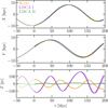 |
Fig. 16 Same as Fig. 13, but for a spiral-perturbed potential with f = 0.3. |
| In the text | |
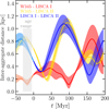 |
Fig. 17 Same as Fig. 14, but for a spiral-perturbed potential with f = 0.3. |
| In the text | |
|
Fig. A.1 Temporal evolution of XYZ galactocentric coordinates for the 15 star clusters in the Perseus complex. Temporal evolution for 500 orbit integrations is shown with background thin lines. The initial conditions were extracted according to the distance and uLOS error distributions. The thicker foreground lines depict the median over multiple integrations. Cluster orbits are color-coded according to the larger cluster agglomerate to which they belong: orange for W345 complex, purple for LISCA I, and green for LISCA II. |
| In the text | |
|
Fig. B.1 Density map on the XY Galactic plane (i.e., computed at Z = 0) for a Galactic potential which includes a tilted rotating bar. |
| In the text | |
|
Fig. B.2 Orbits for the three stellar aggregates studied in this work on the Galactic plane. Orbits were computed within the potential model including the Galactic bar. |
| In the text | |
|
Fig. B.3 Galactocentric coordinate time evolution for the three stellar aggregates studied in this work. Orbits were computed within the potential model including the Galactic bar. The thin lines show the different integrations from the error distribution sampling of the initial conditions, while the thicker lines are the median position at any given time. |
| In the text | |
|
Fig. B.4 3D inter-cluster aggregate distance as a function of time. The orbits were computed in the Galactic potential which includes the bar. |
| In the text | |
|
Fig. C.1 Stellar aggregate orbits on the Galactic plane for three values of f. From left to right f = 0.1, 0.3, 0.5, resulting in stronger density and potential perturbations. The different curves are orbits for different initial conditions extracted according to observed error distributions. The W345, LISCA I, and LISCA II orbits are in orange, purple, and green, respectively. Present-day positions are also shown with filled symbols. |
| In the text | |
|
Fig. C.2 Temporal evolution of galactocentric coordinates for the three cluster aggregates integrated in different spirally perturbed potentials: from left to right f = 0.1, 0.3, 0.5. Darker colors show the forward integration for about 200 Myr, whereas lighter colors show the backward integration. The different colors depict different aggregates: the W345 complex in orange, LISCA I in purple, LISCA II in green. |
| In the text | |
|
Fig. C.3 Inter-aggregate distance evolution for different spirally perturbed potentials. From left to right f = 0.1, 0.3, 0.5. We note the different scales on the y-axis. The gray shaded areas mark the cluster ages range, from 5-30 Myr. |
| In the text | |
Current usage metrics show cumulative count of Article Views (full-text article views including HTML views, PDF and ePub downloads, according to the available data) and Abstracts Views on Vision4Press platform.
Data correspond to usage on the plateform after 2015. The current usage metrics is available 48-96 hours after online publication and is updated daily on week days.
Initial download of the metrics may take a while.