| Issue |
A&A
Volume 698, June 2025
|
|
|---|---|---|
| Article Number | A124 | |
| Number of page(s) | 12 | |
| Section | The Sun and the Heliosphere | |
| DOI | https://doi.org/10.1051/0004-6361/202451855 | |
| Published online | 06 June 2025 | |
Transverse oscillations in 3D along Ca II K bright fibrils in the solar chromosphere
1
Institute for Solar Physics, Dept. of Astronomy, Stockholm University, Albanova University Center, 10691 Stockholm, Sweden
2
Instituto de Astrofísica de Canarias, C/Vía Láctea s/n, 38205 La Laguna, Tenerife, Spain
3
Departamento de Astrofísica, Universidad de La Laguna, 38206 La Laguna, Tenerife, Spain
4
National Solar Observatory, 3665 Discovery Drive, Boulder, CO 80303, USA
⋆ Corresponding authors: This email address is being protected from spambots. You need JavaScript enabled to view it.
, This email address is being protected from spambots. You need JavaScript enabled to view it.
Received:
9
August
2024
Accepted:
7
February
2025
Abstract
Context. Fibrils in the solar chromosphere carry transverse oscillations as determined from non-spectroscopic imaging data. They are estimated to carry an energy flux of several kW m−2, which is a significant fraction of the average chromospheric radiative energy losses.
Aims. We aim to determine the oscillation properties of fibrils not only in the plane-of-the-sky (horizontal) direction, but also along the line-of-sight (vertical) direction.
Methods. We obtained imaging-spectroscopy data in Fe I 6173 Å, Ca II 8542 Å, and Ca II K with the Swedish 1-m Solar Telescope. We created a sample of 605 bright Ca II K fibrils and measured their horizontal motions. Their vertical motion was determined through non-local thermodynamic equilibrium (non-LTE) inversion of the observed spectra. We determined the periods and velocity amplitudes of the fibril oscillations, as well as phase differences between vertical and horizontal oscillations in the fibrils.
Results. The bright Ca II K fibrils carry transverse waves with a mean period of 2.1 × 10² s, and a horizontal velocity amplitude of 1 km s−1, consistent with earlier results. The mean vertical velocity amplitude is 1.1 km s−1. We find that 77% of the fibrils carry waves in both the vertical and horizontal directions, and 80% of this subsample exhibit oscillations with similar periods in both horizontal and vertical directions. For the latter, we find that all phase differences between 0 and 2π occur with a mild but significant preference for linearly polarised waves (a phase difference of 0 or π).
Conclusions. The results are consistent with the scenario where transverse waves are excited by granular buffeting at the photospheric footpoints of the fibrils. Estimates of transverse wave flux based only on imaging data are too low because they ignore the contribution of the vertical velocity.
Key words: Sun: chromosphere / Sun: faculae / plages / Sun: oscillations / Sun: photosphere
© The Authors 2025
 Open Access article, published by EDP Sciences, under the terms of the Creative Commons Attribution License (https://creativecommons.org/licenses/by/4.0), which permits unrestricted use, distribution, and reproduction in any medium, provided the original work is properly cited.
This article is published in open access under the Subscribe to Open model. This email address is being protected from spambots. You need JavaScript enabled to view it. to support open access publication.
1. Introduction
The solar chromosphere is pervaded by waves and oscillations that are excited by the convection and p modes in the photosphere (e.g. Jess et al. 2015, and references therein). These waves are considered prime candidates for transporting the energy needed to sustain chromospheric radiative losses from the photosphere into the chromosphere.
In areas where the gas pressure is stronger than the magnetic pressure (plasma β > 1), acoustic-gravity waves dominate. They are well understood, both observationally and theoretically (e.g. Carlsson & Stein 1997; Wedemeyer et al. 2004), but the extent of their contribution to the required energy input remains under debate (Carlsson et al. 2019). In areas where the magnetic pressure is stronger (β < 1), the situation is more complex. In a homogeneous plasma, there are three waves, the slow and fast magneto-acoustic wave, and the Alfvén wave. The chromosphere is obviously not homogeneous, and a large amount of literature exists about waves in homogeneous magnetic cylinders (referred to as flux tubes in the literature) in which the field is aligned to the axis of the cylinder; these are taken as an approximation of magnetic field bundles (e.g. Edwin & Roberts 1983; Zaqarashvili & Erdélyi 2009; Goossens et al. 2009). In this geometry, there is a complex set of wave modes, including torsional waves, oscillations of the tube diameter (sausage modes), and a swaying of the whole tube (kink modes). The kink mode is the most frequently identified oscillation in observations, as it manifests itself as clearly swaying structures in imagery, especially of spicules that protrude above the limb of the Sun (e.g. De Pontieu et al. 2007; Suematsu et al. 2008).
Propagating transverse oscillations of fibrils and mottles, which are elongated chromospheric structures that emanate from photospheric magnetic elements, have been observed using imaging data in chromospheric spectral lines (Pietarila et al. 2011; Kuridze et al. 2012; Morton et al. 2014; Jafarzadeh et al. 2017). These oscillations have typically been interpreted as kink waves. Observed velocity amplitudes are on the order of 5 km s−1, periods are in the range of 16–600 s, and phase speeds are of 50–300 km s−1. Shetye et al. (2021) studied high frequency waves in spicule-like events using imaging spectroscopy on Hα. In addition to plane-of-the-sky (POS) velocities, they used Doppler shift information to estimate line of sight (LOS) velocity of the spicules. They found periods in the range of 40–200 s, and velocity amplitudes around 5–20 km s−1.
However, when radial and longitudinal inhomogeneities are introduced in magnetic concentrations, the separation of the different wave types becomes more difficult (Srivastava et al. 2021). Radiation magnetohydrodynamic (MHD) models of the chromosphere show that proxies of different wave types often appear in the same location and become indistinguishable (Danilovic et al. 2023).
Leenaarts et al. (2015) investigated the relation between oscillations as seen in Hα imagery and transverse oscillations that propagate along magnetic field lines in a radiation-MHD simulation of a network. They warned that the observed fibrils might not always trace out single field lines, so that interpretation of observations in terms of kink waves along flux tubes must be done with caution. However, radiative transfer computations by Bjørgen et al. (2019) based on a radiation-MHD simulation of an active region, indicate that strong fibrils seen in Hα, Mg II k, and Ca II K trace field lines to a much larger degree than in the network simulations.
There are several observations of transverse oscillations in off-limb spicules using both POS swaying and LOS motions through measuring the Doppler shifts of line profiles (e.g. Gadzhiev & Nikolskii 1982; De Pontieu et al. 2012; Antolin et al. 2018) , but only one where on-limb fibrils are considered (Shetye et al. 2021). In the latter study, Doppler shifts in Hα are used to trace the LOS variations in velocity, which significantly limits the accuracy.
In this paper, we exploit imaging-spectroscopy data obtained at the Swedish 1-m Solar Telescope in multiple spectral lines, combined with non-local thermodynamic equilibrium (non-LTE) inversion, to trace the LOS components as well as the POS components of transverse oscillations. In doing so, we provide a thorough study of the oscillations in 3D, which ensures that the LOS velocity is well resolved.
We focus on oscillations in fibrils that appear bright in Ca II H&K data (Jafarzadeh et al. 2017; Kianfar et al. 2020). The physical properties of these bright fibrils have been studied by Kianfar et al. (2020). We report here on both POS and LOS velocity and displacement amplitudes, wave periods, and correlations between the POS and LOS properties.
2. Observations
2.1. Data preparation
We analysed observations of a fibrillar area centred at ![Mathematical equation: $ (X,Y) = [70{{\overset{\prime\prime}{.}}}4, 153{{\overset{\prime\prime}{.}}}2] $](/articles/aa/full_html/2025/06/aa51855-24/aa51855-24-eq1.gif) , that is, μ = 0.98, taken at the Swedish 1-m Solar Telescope (SST; Scharmer et al. 2003). The observed field of view (FoV) was located at the edge of a plage region in the AR12716. The observations were acquired on 2018 July 22, from 08:23:58 to 08:53:25 UT using the CRisp Imaging Spectro-Polarimeter (CRISP; Scharmer et al. 2008) and CHROMospheric Imaging Spectrometer (CHROMIS; Scharmer 2017) instruments. Seeing conditions were excellent throughout the whole observing time.
, that is, μ = 0.98, taken at the Swedish 1-m Solar Telescope (SST; Scharmer et al. 2003). The observed field of view (FoV) was located at the edge of a plage region in the AR12716. The observations were acquired on 2018 July 22, from 08:23:58 to 08:53:25 UT using the CRisp Imaging Spectro-Polarimeter (CRISP; Scharmer et al. 2008) and CHROMospheric Imaging Spectrometer (CHROMIS; Scharmer 2017) instruments. Seeing conditions were excellent throughout the whole observing time.
The Fe I 6173 Å line was sampled by CRISP in 13 equidistant wavelength positions in a range of ±180 mÅ around the line centre. CRISP also observed the Ca II 8542 Å line. It was sampled at 21 equidistant wavelength positions between ±550 mÅ, as well as two extra points at ±880 Å from the line core. Both lines were observed with full Stokes polarimetry and with a total cadence of 21 s.
The Ca II K line was observed by CHROMIS in 27 equidistant wavelength positions in the range ±1.5 Å around the line core. In addition, it observed an additional wavelength point at 4000 Å (continuum). The CHROMIS observations have a cadence of 8 s.
We reconstructed the observed data by applying the CRISPRED reduction pipeline (de la Cruz Rodríguez et al. 2015) to the CRISP data and SSTRED (Löfdahl et al. 2021) to the CHROMIS observations. The image restoration used in the reconstruction pipelines is the multi-object multi-frame blind deconvolution (MOMFBD; van Noort et al. 2005) method. After reconstruction, the CRISP and CHROMIS images were co-aligned with an accuracy of about 0.1 pixel. The CRISP data were resampled from a pixel size of  to the CHROMIS pixel size of 0
 038. They were also resampled in time to the CHROMIS cadence using nearest-neighbour interpolation. The data were calibrated to the absolute intensity by comparing the average intensity profile in a quiet region in the FoV to a solar atlas profile (Neckel & Labs 1984).
2.2. Overview of the FoV
Figure 1 and the accompanying animation show an overview of the observations. The upper-left corner of the FoV contains a plage region with a concentration of unipolar small-scale magnetic features as seen in the linear and circular polarisation maps (Figs. 1c and 1d). The area surrounding the plage region is covered with a forest of elongated bright fibrils in the chromosphere (Fig. 1b). The Ca II 8542 Å line core image in Fig. 1e shows a fibrillar pattern similar to the one in Ca II K (cf. Fig. 1f, Kianfar et al. 2020). The right half of the CHROMIS FoV is quiet and therefore devoid of bright fibrils as shown in the Ca II K continuum image in Fig. 1a. We used this part of the FoV for the absolute intensity calibration of our observations (see Sect. 2.1).
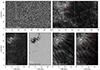 |
Fig. 1. Overview of the observations taken on 2018 July 22 at 08:31:49 UT. The top panels show intensity images of the continuum at 4000 Å (a) and the wavelength-integrated Ca II K line intensity (b). The dashed white box marks the region that we analyse in detail. The red box marks the region of interest (RoI) analysed in Fig. 3. A zoom-in of the area enclosed by the dashed white box is shown in the bottom panels. (c) Fe I 6173 Å wavelength-averaged linear polarisation; (d) Fe I 6173 Å wavelength-averaged circular polarisation; (e) Ca II 8542 Å line core intensity; (f) Ca II K line core intensity. The solid red and dashed white lines in panel (f) show the cuts across the Ca II K bright fibrils that we used (see Sect. 3.1). An analysis of the cut along the dashed white line is presented in Figs. 7 and 8. The white dot marks the zero point on the y-axis in Fig. 7. An animated version of this figure showing the entire time sequence is available online. |
3. Analysis methods
3.1. Measuring POS oscillations
In order to analyse the transverse (POS) oscillations of bright fibrils visible in Ca II K, we selected a region in our data that was observed by both CRISP and CHROMIS and contained fibrils (indicated by the white-dashed box in Fig. 1b). Then we defined 12 cuts of 3″ − 12″ in length perpendicular to the local orientation of the fibrils in this region using the CRisp SPectral EXplorer computer program (CRISPEX; Vissers & Rouppe van der Voort 2012; Löfdahl et al. 2021).
The space-time Ca II intensity plots of the cross-cuts reveal the oscillations of the bright fibrils (see panel (a) of Fig. 2 for an example). In order to bring out the oscillations more clearly, we processed the intensity data following the steps below, similar to the processes used by Kianfar et al. (2020) and Jafarzadeh et al. (2013, 2017):
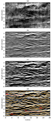 |
Fig. 2. Time evolution of the cut across the bright fibrils shown with a dashed white line (Fig. 1f). Panel (a) displays the intensity at the nominal line centre of Ca II K. Panel (b) shows the enhanced intensity of panel (a) by applying the enhancing procedure described in Sect. 3.1. Panel (c) is the gamma-corrected image of panel (b) that fully brings out individual fibril oscillations. The POS oscillation trajectories are marked on the high contrast space-time image in panel (d), where the preliminary paths are plotted with dashed lines and the smoothed oscillations are plotted with solid curves. The oscillation properties of the curves marked with numbers are shown in Fig. 8. The zero point of the cut length (y-axis) is marked with a white dot in Fig. 1f. |
-
We integrated the intensity over the wavelength span that includes Ca II K2 peaks and the line core.
-
We subtracted the wavelength-averaged wing intensity from the integrated core image to suppress the lower chromospheric contribution, in particular the 3-min acoustic oscillations.
-
We applied unsharp masking in the time direction using a median kernel of three pixels wide to lower residual image jitter.
Figures 2a and 2b show the space-time intensity plots of an example cross-cut before and after the above enhancement procedure.
We defined the trajectory of the POS oscillations in the processed space-time plots using a combination of manual and automatic approaches. First, we manually defined a preliminary trail of each oscillation by choosing a sparse set of (x, t) points along the oscillating fibril. Second, we linearly interpolated in time between these points to get a preliminary rough oscillation curve. Third, for each time step, similar to Kuridze et al. (2012), we applied a Gaussian fit to the intensity at each time step around the preliminarily defined fibril location to get the precise location of the fibril. Finally, we smoothed the oscillation trajectories by applying a 1D boxcar average in time with a width of 64 seconds (eight time steps) to remove fluctuations on short timescales. We note that this smoothing introduces a bias in our sample by eliminating the oscillations with short periods. However, this does not affect our results as we are focusing on longer periods.
Using the above procedure, we created a sample of 605 POS oscillations of Ca II K bright fibrils. The bottom panel of Fig. 2 shows the interpolated and smoothed trajectories of POS oscillations in the example cut marked in Fig. 1f. The fitted fibril curves follow the unsmoothed fibrils in the background image rather well, which gives us confidence that the smoothing in time does not bias our results too strongly.
We calibrated the overall axis of the oscillations by subtracting a linear trend from the trajectories so that the oscillation axis becomes parallel to the time axis (Leenaarts et al. 2015). Then we computed the velocity of the POS oscillations by calculating the time derivative of the amplitudes.
3.2. Inversion and measurement of LOS oscillations
We used the Message Passing Interface (MPI)-parallel STockholm inversion Code (STiC; de la Cruz Rodríguez et al. 2019) to derive the physical properties of the atmosphere from our observations. We used the inferred atmospheric velocity to estimate the LOS velocity in our fibril sample.
To solve the polarised radiative transfer equation, STiC uses the radiative transfer code RH (Uitenbroek 2001) with Bezier solvers (de la Cruz Rodríguez & Piskunov 2013). STiC uses the equation-of-state that is acquired from the Spectroscopy Made Easy (SME) package functions (Piskunov & Valenti 2017), and includes partial redistribution (PRD) effects in the radiative transfer using the fast approximation method introduced in Leenaarts et al. (2012b). STiC fits multiple spectral lines simultaneously for each individual pixel by assuming the 1.5D approximation (i.e. plane-parallel atmosphere). We ran STiC on the observations of the three Fe I 6173 Å, Ca II 8542 Å, and Ca II K lines to retrieve the physical properties in both the photosphere and chromosphere. In our inversion runs, we assumed the statistical equilibrium and non-LTE condition for Ca II, including partial redistribution for the Ca II K line. For the Fe I 6173 Å line, we assumed LTE.
We did not aim to determine the magnetic field, and therefore only fitted Stokes I, even though our observations included all four Stokes parameters for Fe I 6173 Å and Ca II 8542 Å. Because Zeeman broadening affects the width and shape of the line profiles, in particular for Fe I 6173 Å, we included the longitudinal magnetic field as a quantity in our atmospheric model with two nodes, and the transverse field with one node. Otherwise we used the same set-up and nodes to run the inversions as used in Kianfar et al. (2020), who used nine nodes in temperature, and four nodes for both vLOS and vturb, located non-equidistantly in the optical depth span of log(τ500 nm) = [ − 7, 1]. The inversion results are presented in Section 4.1.
4. Results
4.1. Inversion results
4.1.1. Region of interest
To study the time-evolution of the fibrils, we first ran inversions on the time series of a 2D region marked by the red box in Fig. 1b. The results are shown in Fig. 3. The region of interest (RoI) covers an area of  that centres on a long-lived fibril (Fig. 3, Ca II K image at 22 minutes) with a clear transverse oscillation. The temperature and vLOS images in the photosphere (i.e. log(τ500 nm) = 0) show a convection pattern consistent with the granulation pattern in the intensity images; there is a higher temperature and upflows in the granules, and a lower temperature and downflows in the intergranular lanes. The temperature in log(τ500 nm) = −3.9 at t = 10 min and t = 18 min almost follows the fibrillar patterns of the intensity images at Ca II 8542 Å line-core. The fibrillar patterns in the temperature become more significant at log(τ500 nm) = −4.6 in the chromosphere, where the bright fibrils appear as temperature enhancements in agreement with the Ca II K intensity images (Kianfar et al. 2020). The upflow and downflow structures in the vLOS images in the chromosphere do not particularly follow the fibrillar patterns, though they have the same average orientation as the fibrils (Kianfar et al. 2020).
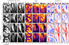 |
Fig. 3. Time evolution of the physical properties of the RoI marked with a red box in Fig. 1. Left panels: Intensity variation over time (from top to bottom) at the 4000 Å continuum, and in the line cores of Ca II 8542 Å and Ca II K. Middle and right panels: Time evolution of the temperature and vLOS at a photospheric depth (log(τ500 nm) = 0.1) and two different chromospheric depths, log(τ500 nm) = −3.9 and −4.6. Three cuts across the head, middle, and the tail of this fibril are marked and numbered and their properties as a function of time are displayed in Fig. 4. |
We chose three perpendicular cuts (the dashed lines in Fig. 3) across the central fibril in the RoI. Figure 4 shows space-time plots of the intensity and inversion results along these cuts. The optical depth at which the inversion results are extracted is log(τ500 nm) = −4.3 because the Ca II K line is most sensitive to the perturbations in the chromosphere at this optical depth (Kianfar et al. 2020). The smoothed interpolated trajectories of the fibrillar POS oscillations in the cross-cuts are defined by the method explained in Sect. 3.1 (overplotted curves in Fig. 4). They exhibit oscillations with a period, P, of about 12 minutes that last for two periods. The period stays roughly constant along the fibril. We calculated the average phase speed for the oscillation along this fibril as
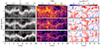 |
Fig. 4. Physical properties of the cross-cuts marked in Fig. 3. The left column shows the intensity-over-time variations of the cuts at the Ca II K nominal line centre. The oscillation in the POS is marked by dotted red curves. The middle and right columns display the temperature and vLOS variations of the cuts as a function of time in the chromosphere (log(τ500 nm) = −4.31). The POS oscillation is overplotted on these images as well. Length zero on the y-axis is where the cuts are marked by numbers in Fig. 3. The vertical line (|) symbols, marked on the curves in the left column, show the specific times of the fibril’s evolution that are displayed in Fig. 3. |
 (1)
(1)
where Δr is the average distance between the cuts and Δtϕc is the average time difference between the two points that have the same phase in the oscillations. Accordingly the wave along this fibril propagates with an average speed of ∼12 km s−1 from cut 1 to cut 3. The amplitude of the oscillations is highest ( ) at the head of the fibril (i.e. close to the magnetic field concentration, top panels of Fig. 4) and it decreases to
  in the tail.
The temperature (middle column of Fig. 4) almost follows the oscillatory patterns in intensity, with enhancements of 40–60 K. There are no obvious wave patterns in vLOS.
We extracted the temperature and vLOS along the POS oscillations in the cuts of Fig. 4 in the atmosphere between log(τ500 nm) = [ − 6, −2]. This is roughly the height range where the Ca II K line responds to perturbations in the physical properties in the atmosphere (Kianfar et al. 2020). The results are shown in Fig. 5. The oscillatory pattern in vLOS (right panel) starts around log(τ500 nm) ∼ −2.5 and increases at greater heights, peaking between log(τ500 nm) = [ − 3, −6]. The temperature profiles (left panel) do not show any particular wave patterns.
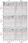 |
Fig. 5. Temperature (left column) and vLOS (right column) variations of the three cuts marked in Fig. 3 over time. The panels show the temperature and vLOS variations along the POS oscillation trajectory (marked in Fig. 4) for a depth range where Ca II K is sensitive to the perturbations in the atmosphere. Solid curves are the smoothed plots of the actual values that are shown with dots. Red curves mark the depth where Ca II K has the highest sensitivity to atmospheric perturbations. These curves are plotted individually in Fig. 6. |
However, there are peaks forming at t = 11 and 19 minutes, which is where the POS amplitude has extrema (see Fig. 4). These temperature peaks start appearing above log(τ500 nm) = −4 and get stronger up to log(τ500 nm) = −5. Higher up, they get damped. This optical depth range is where bright Ca II K fibrils show temperature enhancements compared to their surroundings (Kianfar et al. 2020).
While the peaks in the temperature profiles get smaller as we move towards the tail of the fibril (i.e. from cut 1 to cut 3), the amplitude of vLOS oscillations increases. Figure 6 shows a comparison of the time evolution of T and vLOS at log(τ500 nm) = −4.31 to vPOS. It shows that both the temperature variation and its average decrease as we move from the head to the tail of the fibril. The amplitude of vPOS behaves the same. The vLOS curves show different behaviour, with the highest amplitude peak at about t = 16 min in cut 3, which is close to the tail of the fibril. We further discuss the vPOS and vLOS oscillations of our sample and their wave properties in Sect. 4.2.
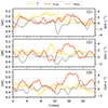 |
Fig. 6. Variations of the temperature (yellow line) and vLOS (orange line) of the perpendicular cross-cuts shown in Fig. 3. They are plotted based on their values extracted along the oscillation trajectory in POS marked in Fig. 4 at the depth log(τ500 nm) = −4.31 (i.e. where the Ca II K line is most sensitive to atmospheric perturbations). The oscillation of vPOS is plotted in grey for comparison. |
4.1.2. Cross-cuts
Figure 7 shows the temperature and vLOS of the example cut shown in Fig. 2 at two chromospheric heights. The temperature in the lower chromosphere (log τ500 = −3.5) demonstrates a very faint pattern of fibrillar structures. Higher up, at log τ500 = −4.31, the temperature image shows more recognisable fibrillar structures that resemble similar patterns to the space-time intensity image (Fig. 2) with enhanced temperature at the location of the bright fibrils (Kianfar et al. 2020). The vLOS space-time images do not demonstrate a clear correlation to the fibrillar oscillation trajectories in the POS and appears similar at both heights, with only a slight difference in the range of the velocity values.
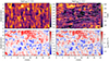 |
Fig. 7. Time evolution of the physical properties of the example cross-cut shown in Fig. 2. The left column shows the inversion results in the lower chromosphere and the right column represents the results higher in the chromosphere. The top panels show the temperature of the cut in the chromosphere. The bottom panels show space-time images of the LOS velocity. The POS oscillations are overplotted on the right panels. The zero point of the cut length is marked with a white dot in Fig. 1. |
4.2. Three-dimensional oscillations
From the POS oscillation trajectories (Sect. 3.1) and space-time inversion results of the cuts across the fibrils (Sect. 4.1.2), we determined the LOS velocity along the fibrils. To do so, we extracted the vLOS values along the smoothed trajectory of the POS oscillations (Sect. 3.1) at log(τ500 nm) = −4.31, which is the height where temperature and velocity at fibrillar locations are most sensitive to the perturbations in the chromosphere (Kianfar et al. 2020). In addition, we computed the velocity in the POS by taking the time derivative of the POS displacement. The top panels of Fig. 8 show vLOS an vPOS along the four example fibrils marked with numbers in Fig. 2.
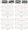 |
Fig. 8. Comparison of the velocity oscillations of the four examples marked with numbers in Fig. 2. These examples represent four different groups of oscillations in our sample of Ca II K fibrillar oscillations. The top row shows time slices of the example fibrils, with the smoothed fitted POS motion overplotted with dotted red curves. Below, we show three plots for each of the four fibrils. The top plot shows the POS velocity (red), and the LOS velocity (grey) with a solid curve for the smoothed data and a dotted curve for the unsmoothed data. The middle plot shows the auto-correlation function of the POS (grey) and the LOS (red) velocity. The bottom plot shows the normalised cross-correlation function ( |

4.2.1. Determination of the oscillation properties
We derived the wave properties in our oscillation sample through a combination of automatic and manual approaches. First, we computed the autocorrelation of each vLOS and vPOS curve. Besides the peak at a time lag Δt = 0 s, a curve with an oscillation shows a secondary peak at a time lag roughly equal to the dominant period of the oscillation. Because the velocity curves contain noise, and might contain partial oscillations, interference patterns, or oscillation with changing period, the secondary peak can have a much lower amplitude. Combining the autocorrelations with direct visual inspection of the curves, we found a subsample of 468 fibrils out of the total sample size of 605 that have a clear oscillation in both vLOS and vPOS. The middle panels of Fig. 8 show the autocorrelations for the four example fibrils marked with numbers in Fig. 2 that belong to this category.
We then derived periods for this subsample by measuring the time of each extremum, and computed ‘partial periods’ as the time difference between two consecutive minima or maxima. As the periods are not constant throughout one oscillation, we assigned an average and a dominant period ( , Pdom) as the mean and maximum of the partial periods for vLOS and vPOS in each fibril. We also measured the amplitude of each extremum, and used that to assign an average amplitude
  for vLOS and vPOS for each oscillation.
To quantify the correlation between vLOS and vPOS, we calculated the normalised cross-correlation function,  , for each fibril. Cross-correlation curves of the example fibrils are shown in the bottom panels of Fig. 8. We considered fibrils with
  as potentially exhibiting correlated motion. Then we visually inspected those fibrils to confirm that vLOS and vPOS indeed have similar periods and oscillation patterns. Those fibrils with a sufficiently high
  and a difference in period between the two velocity components smaller than 20% defined a subset of 373 fibrils out of the 468 oscillations.
For this subset, we computed the phase difference between the oscillations as
 (2)
(2)
where  . The online animation accompanying Fig. 8 shows all fibrils in our subset.
4.2.2. Statistical analysis
Figure 9 shows the distribution of and correlations between the measured periods and amplitudes. Table 1 shows their minimum, maximum, average, and standard deviation.
The top-left panel of Fig. 9 shows a weak but positive correlation between  and
and  , especially between periods of 130–210 s. In contrast, the amplitudes (lower-left panel) do not appear to have a correlation between the two POS and LOS directions. In general, the vLOS oscillations tend to have slightly larger amplitudes compared to vPOS. This is also confirmed by the mean values in Table 1. There appears to be no correlation between the amplitude and period in the POS direction (upper right), and likewise for the LOS direction (lower right).
Statistic summary of the fibril oscillations along LOS and POS directions.
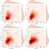 |
Fig. 9. Kernel density estimate (KDE) plots and histograms of the average period, |


We show the distribution of the phase difference between the vPOS and vLOS oscillations for the 373 fibrils in our sample that indicate correlated velocity oscillations in the POS and LOS directions in Figure 10. The observed phase difference spans the whole range of [−π, π]. This implies that the total velocity vectors vtot = (vPOS, vLOS) can range from fully linearly polarised (Δϕ = 0, −π, or π) to fully circularly polarised (Δϕ = ±π/2).
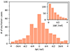 |
Fig. 10. Distribution of the phase difference Δϕ and |Δϕ| for the 373 fibrils in our sample that show velocity oscillations in the POS and LOS direction with similar periods. |
We also show the distribution of |Δϕ| in Fig. 10. Because our sample size is limited and we are only interested in absolute phase differences, this lowers the statistical noise in our sample. There is a clear peak in the distribution for linearly polarised waves.
In order to visualise the motion of the fibril in 3D, we integrated the LOS velocity to obtain the LOS displacement as a function of time. Together with the measured POS amplitude, we can then trace the motion of a particular point along a fibril as a function of time. We display these curves in Fig. 11 for the four example fibrils shown in Figs. 2 and 8.
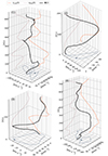 |
Fig. 11. Time evolution of the motion of a point along the fibril axis A(t) of the four example oscillations shown in Figs. 2 and 8. The oscillations in the POS and LOS are shown in the side planes and the projections of the total motion are plotted in the plane perpendicular to the POS and LOS. The small arrow shows the direction of the motion in the bottom plane. An animated version of this figure showing all 468 correlated fibrils in our sample is available online. |
The phase differences between the velocity oscillations of examples (1) and (2) are 0 and π as shown in Fig. 8, which suggests a linear polarised wave. This linear behaviour is seen roughly in the total motion of example (2) in Fig. 11 but not so clearly in example (1). Example (3) has a Δϕ ≈ π/2, and therefore the projection of the amplitude vector traces out an elliptical path. Example (4) has velocities that appeared to be low-amplitude short-period velocities with different periods in the LOS and POS directions. However, the projection of the amplitude vector reveals that it carried a long-period linear oscillation as well as the short period oscillations.
Finally, we investigated the spatial distribution of the periods and phase differences. Our results are shown in Fig. 12. There is no correlation between the location of the fibril cross-cuts and their periods and phase difference.
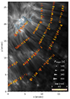 |
Fig. 12. Spatial distribution of measured fibril oscillation periods and LOS-POS phase differences. Each symbol marks the coordinates of the oscillation point. The triangular symbols mark the points where an oscillation is detected in both vPOS and vLOS. The size of the triangular symbols is proportional to their average period. The colour-coding of yellow, orange, and red represents the absolute values of the phase difference between the vLOS and vPOS oscillations where their period is correlated. The coordinates of the oscillations that do not have a clear correlation between their |


Summary of results. We now present a summary of our main findings. We selected a number of cross-cuts through Ca II K bright fibrils, and defined a sample of 605 fibrils along these cross-cuts. We determined the velocity amplitudes and periods of the fibril oscillations for both the LOS and POS directions. The distribution of periods and amplitudes in both directions is similar, with a mean period of around 2.2 × 10² s, and a mean velocity amplitude of 1.1 km s−1.
Because the sample was selected based on POS oscillations, all of them exhibit a POS oscillation. The majority of them (77%, i.e. 468 fibrils out of 605 oscillations in total) show a clear LOS oscillation pattern. Of those, 373 fibrils (80% of the subsample) showed oscillations with similar periods in both the LOS and POS directions. For these, we measured the phase difference between the two oscillation directions. All phase differences occur, but there is a preference for zero phase difference.
5. Discussion
The periods and POS velocity amplitudes that we measure here fall in the range of transverse oscillations observed in Hα fibrils as reported by Morton et al. (2013). The oscillations in Hα spicule-like events reported by Shetye et al. (2021) have smaller periods and larger amplitudes.
The median period in POS oscillations of about 190 s that we measure is larger than the median period of 84 s reported in Jafarzadeh et al. (2017) for Ca II H fibrils observed with a 0.11 nm filter. Table 2 of Jafarzadeh et al. (2017) lists the observed periods and amplitudes of transverse oscillations in fibrils, mottles, and spicules observed in Hα and Ca II H in different studies using a variety of instruments. Specifically, the observed periods ranged between 16 s and 600 s, and was roughly consistent for all studies. However, the differences in periods and amplitudes might have multiple causes, such as differences in the observed target, observing cadence, procedures used to define and detect spicules, and data processing. A limit upon our study is that we smooth oscillations in time with a 64 s boxcar average, which effectively blocks us from detecting periods smaller than ∼120 s. This might explain the larger value for the median period that we found compared to those in Jafarzadeh et al. (2017) and Shetye et al. (2021). While the use of a 64 s boxcar filter was employed to remove residual instrumental jitter, we acknowledge that even though a 64 s boxcar filter was employed filtering which causes not to fully exploit the high cadence of the data, the smaller scale higher frequency oscillations were not the subject of our study.
Observations of fibrils in Hα and Type II spicules show diverse velocity amplitudes, with median values ranging from 5 km s−1 to 10 km s−1. The Ca II K fibrils in this study, as well as those observed by Jafarzadeh et al. (2017), have a POS velocity amplitude in the range of 1–2 km s−1. This difference could be explained by the differences in the formation height together with decreasing mass density with height: for constant wave flux (and phase speed), lower density gas implies larger velocity amplitude. For fibrils that appear both in Ca II K and Hα, the segment of the fibril that appears bright in Ca II K is likely located lower in the atmosphere than the segment only visible in Hα. Kianfar et al. (2020) reported that Ca II K shows fibrils located around log τ500 ≈ −4.3, while the Hα line core forms at larger heights (log τ500 ≈ −5.7 in the Fontenla, Avrett, and Loeser C (FALC) model atmosphere). Type II spicules can protrude far above the bulk chromosphere and are expected to form at even lower densities.
The presence of oscillations in both the LOS and POS direction, with comparable periods for 373 out of 468 fibrils in our sample, strongly suggests that both oscillation directions are excited by the same process. Theoretical calculations show that curved flux tubes have nearly the same wave speeds in the vertical and horizontal directions (van Doorsselaere et al. 2009).
The presence of fibrils with identical periods and zero phase difference in our sample is consistent with convective buffeting (Spruit 1981) that has randomly oriented kicks as a driver because there is only a very weak correlation between the LOS and POS velocity amplitudes (Fig. 9). We note that the three-minute oscillations, often linked to larger magneto-acoustic waves, may influence the LOS velocity. However, Rosenthal et al. (2002) suggest that these oscillations do not penetrate deeply into the β < 1 regime, where the bright fibrils are located, thus minimising their potential impact on our analysis.
However, simulations of photospheric magnetoconvection at high resolution (e.g. Rempel 2014) show substantially more complex motions of photospheric magnetic elements, which could explain the whole range of phase differences that we observe. We find similar velocity amplitudes for the POS and the LOS oscillations. Shetye et al. (2021) found smaller LOS amplitudes than POS amplitudes in Hα spicules. They defined the LOS velocity as the first moment of the line profile, which can yield different values than the actual LOS gas velocity (see Figs. 5 and 6 in Danilovic et al. 2023). The measurement of fibril oscillations in Hα using the Doppler shift of the line profile minimum as a LOS velocity measurement (Leenaarts et al. 2012a) could provide a more reliable measurement of the relative sizes of the LOS and POS velocity amplitudes.
The existence of fibrils with a phase difference of π/2 between the oscillations in POS and LOS directions indicates the presence of fully circularly polarised waves, in the context of flux tubes known as helical kink waves (Zaqarashvili & Skhirtladze 2008). This leads to circular motion of the tube axis in the plane perpendicular to the tube. Such motions have been detected before in both off-limb spicules (e.g. Gadzhiev & Nikolskii 1982) and on-disc spicules (Shetye et al. 2021). Similar motions have also been detected in the chromosphere above photospheric magnetic elements using feature tracking (Stangalini et al. 2017).
Finally, we note that estimates of the wave flux carried by transverse waves in chromospheric fibrils based on POS motions only are an underestimate because they do not include the significant LOS motions. As we show here, imaging spectroscopy, together with non-LTE inversions, is a powerful tool to study chromospheric oscillations in all three dimensions.
Data availability
Movies associated to Figs. 1, 8, 11 are available at https://www.aanda.org
Acknowledgments
SK and JL were supported through the CHROMATIC project (2016.0019) funded by the Knut and Alice Wallenberg foundation. SEP was supported by the Knut and Alice Wallenberg Foundation and also acknowledges the funding received from the European Research Council (ERC) under the European Union’s Horizon 2020 research and innovation program (ERC Advanced Grant agreement No. 742265) and from the Agencia Estatal de Investigación del Ministerio de Ciencia, Innovación y Universidades (MCIU/AEI) under grant “Polarimetric Inference of Magnetic Fields” and the European Regional Development Fund (ERDF) with reference PID2022-136563NB-I00/10.13039/501100011033. SD has received funding from Swedish Research Council (2021-05613) and Swedish National Space Agency (2021-00116). The Swedish 1-m Solar Telescope is operated on the island of La Palma by the Institute for Solar Physics of Stockholm University in the Spanish Observatorio del Roque de los Muchachos of the Instituto de Astrofísica de Canarias. The Institute for Solar Physics is supported by a grant for research infrastructures of national importance from the Swedish Research Council (registration number 2021-00169). This project has received funding from the European Research Council (ERC) under the European Union’s Horizon 2020 research and innovation program (SUNMAG, grant agreement 759548). The NSO is operated by the Association of Universities for Research in Astronomy, Inc., under cooperative agreement with the National Science Foundation.
References
- Antolin, P., Schmit, D., Pereira, T. M. D., De Pontieu, B., & De Moortel, I. 2018, ApJ, 856, 44 [Google Scholar]
- Bjørgen, J. P., Leenaarts, J., Rempel, M., et al. 2019, A&A, 631, A33 [Google Scholar]
- Carlsson, M., & Stein, R. F. 1997, ApJ, 481, 500 [Google Scholar]
- Carlsson, M., De Pontieu, B., & Hansteen, V. H. 2019, ARA&A, 57, 189 [Google Scholar]
- Danilovic, S., Bjørgen, J. P., Leenaarts, J., & Rempel, M. 2023, A&A, 670, A50 [NASA ADS] [CrossRef] [EDP Sciences] [Google Scholar]
- de la Cruz Rodríguez, J., & Piskunov, N. 2013, ApJ, 764, 33 [Google Scholar]
- de la Cruz Rodríguez, J., Löfdahl, M. G., Sütterlin, P., Hillberg, T.& Rouppe van der Voort, L. 2015, A&A, 573, A40 [NASA ADS] [CrossRef] [EDP Sciences] [Google Scholar]
- de la Cruz Rodríguez, J., Leenaarts, J., Danilovic, S., & Uitenbroek, H. 2019, A&A, 623, A74 [Google Scholar]
- De Pontieu, B., McIntosh, S. W., Carlsson, M., et al. 2007, Science, 318, 1574 [Google Scholar]
- De Pontieu, B., Carlsson, M., Rouppe van der Voort, L. H. M., et al. 2012, ApJ, 752, L12 [Google Scholar]
- Edwin, P. M., & Roberts, B. 1983, Sol. Phys., 88, 179 [Google Scholar]
- Gadzhiev, T. G., & Nikolskii, G. M. 1982, Sov. Astron. Lett., 8, 341 [Google Scholar]
- Goossens, M., Terradas, J., Andries, J., Arregui, I., & Ballester, J. L. 2009, A&A, 503, 213 [NASA ADS] [CrossRef] [EDP Sciences] [Google Scholar]
- Jafarzadeh, S., Solanki, S. K., Feller, A., et al. 2013, A&A, 549, A116 [NASA ADS] [CrossRef] [EDP Sciences] [Google Scholar]
- Jafarzadeh, S., Solanki, S. K., Gafeira, R., et al. 2017, ApJS, 229, 9 [Google Scholar]
- Jess, D. B., Morton, R. J., Verth, G., et al. 2015, Space Sci. Rev., 190, 103 [Google Scholar]
- Kianfar, S., Leenaarts, J., Danilovic, S., de la Cruz Rodríguez, J., & José Díaz Baso, C. 2020, A&A, 637, A1 [NASA ADS] [CrossRef] [EDP Sciences] [Google Scholar]
- Kuridze, D., Morton, R. J., Erdélyi, R., et al. 2012, ApJ, 750, 51 [NASA ADS] [CrossRef] [Google Scholar]
- Leenaarts, J., Carlsson, M., & Rouppe van der Voort, L. 2015, ApJ, 802, 136 [NASA ADS] [CrossRef] [Google Scholar]
- Leenaarts, J., Carlsson, M., & Rouppe van der Voort, L. 2012a, ApJ, 749, 136 [NASA ADS] [CrossRef] [Google Scholar]
- Leenaarts, J., Pereira, T., & Uitenbroek, H. 2012b, A&A, 543, A109 [NASA ADS] [CrossRef] [EDP Sciences] [Google Scholar]
- Löfdahl, M. G., Hillberg, T., de la Cruz Rodríguez, J., et al. 2021, A&A, 653, A68 [Google Scholar]
- Morton, R. J., Verth, G., Fedun, V., Shelyag, S., & Erdélyi, R. 2013, ApJ, 768, 17 [Google Scholar]
- Morton, R. J., Verth, G., Hillier, A., & Erdélyi, R. 2014, ApJ, 784, 29 [NASA ADS] [CrossRef] [Google Scholar]
- Neckel, H., & Labs, D. 1984, Sol. Phys., 90, 205 [Google Scholar]
- Pietarila, A., Aznar Cuadrado, R., Hirzberger, J., & Solanki, S. K. 2011, ApJ, 739, 92 [NASA ADS] [CrossRef] [Google Scholar]
- Piskunov, N., & Valenti, J. A. 2017, A&A, 597, A16 [NASA ADS] [CrossRef] [EDP Sciences] [Google Scholar]
- Rempel, M. 2014, ApJ, 789, 132 [Google Scholar]
- Rosenthal, C. S., Bogdan, T. J., Carlsson, M., et al. 2002, ApJ, 564, 508 [NASA ADS] [CrossRef] [Google Scholar]
- Scharmer, G. 2017, in SOLARNET IV: The Physics of the Sun from the Interior to the Outer Atmosphere, 85 [Google Scholar]
- Scharmer, G. B., Bjelksjo, K., Korhonen, T. K., Lindberg, B., & Petterson, B. 2003, in Innovative Telescopes and Instrumentation for Solar Astrophysics, eds. S. L. Keil, & S. V. Avakyan, Proc. SPIE, 4853, 341 [NASA ADS] [CrossRef] [Google Scholar]
- Scharmer, G. B., Narayan, G., Hillberg, T., et al. 2008, ApJ, 689, L69 [Google Scholar]
- Shetye, J., Verwichte, E., Stangalini, M., & Doyle, J. G. 2021, ApJ, 921, 30 [Google Scholar]
- Spruit, H. C. 1981, A&A, 98, 155 [NASA ADS] [Google Scholar]
- Srivastava, A. K., Ballester, J. L., Cally, P. S., et al. 2021, J. Geophys. Res. (Space Phys.), 126, e029097 [NASA ADS] [Google Scholar]
- Stangalini, M., Giannattasio, F., Erdélyi, R., et al. 2017, ApJ, 840, 19 [NASA ADS] [CrossRef] [Google Scholar]
- Suematsu, Y., Ichimoto, K., Katsukawa, Y., et al. 2008, in First Results From Hinode, eds. S. A. Matthews, J. M. Davis, & L. K. Harra, ASP Conf. Ser., 397, 27 [Google Scholar]
- Uitenbroek, H. 2001, ApJ, 557, 389 [Google Scholar]
- van Doorsselaere, T., Verwichte, E., & Terradas, J. 2009, Space Sci. Rev., 149, 299 [NASA ADS] [CrossRef] [Google Scholar]
- van Noort, M., Rouppe van der Voort, L., & Löfdahl, M. G. 2005, Sol. Phys., 228, 191 [Google Scholar]
- Vissers, G., & Rouppe van der Voort, L. 2012, ApJ, 750, 22 [Google Scholar]
- Wedemeyer, S., Freytag, B., Steffen, M., Ludwig, H. G., & Holweger, H. 2004, A&A, 414, 1121 [NASA ADS] [CrossRef] [EDP Sciences] [Google Scholar]
- Zaqarashvili, T. V., & Erdélyi, R. 2009, Space Sci. Rev., 149, 355 [NASA ADS] [CrossRef] [Google Scholar]
- Zaqarashvili, T. V., & Skhirtladze, N. 2008, ApJ, 683, L91 [Google Scholar]
All Tables
All Figures
|
Fig. 1. Overview of the observations taken on 2018 July 22 at 08:31:49 UT. The top panels show intensity images of the continuum at 4000 Å (a) and the wavelength-integrated Ca II K line intensity (b). The dashed white box marks the region that we analyse in detail. The red box marks the region of interest (RoI) analysed in Fig. 3. A zoom-in of the area enclosed by the dashed white box is shown in the bottom panels. (c) Fe I 6173 Å wavelength-averaged linear polarisation; (d) Fe I 6173 Å wavelength-averaged circular polarisation; (e) Ca II 8542 Å line core intensity; (f) Ca II K line core intensity. The solid red and dashed white lines in panel (f) show the cuts across the Ca II K bright fibrils that we used (see Sect. 3.1). An analysis of the cut along the dashed white line is presented in Figs. 7 and 8. The white dot marks the zero point on the y-axis in Fig. 7. An animated version of this figure showing the entire time sequence is available online. |
| In the text | |
|
Fig. 2. Time evolution of the cut across the bright fibrils shown with a dashed white line (Fig. 1f). Panel (a) displays the intensity at the nominal line centre of Ca II K. Panel (b) shows the enhanced intensity of panel (a) by applying the enhancing procedure described in Sect. 3.1. Panel (c) is the gamma-corrected image of panel (b) that fully brings out individual fibril oscillations. The POS oscillation trajectories are marked on the high contrast space-time image in panel (d), where the preliminary paths are plotted with dashed lines and the smoothed oscillations are plotted with solid curves. The oscillation properties of the curves marked with numbers are shown in Fig. 8. The zero point of the cut length (y-axis) is marked with a white dot in Fig. 1f. |
| In the text | |
|
Fig. 3. Time evolution of the physical properties of the RoI marked with a red box in Fig. 1. Left panels: Intensity variation over time (from top to bottom) at the 4000 Å continuum, and in the line cores of Ca II 8542 Å and Ca II K. Middle and right panels: Time evolution of the temperature and vLOS at a photospheric depth (log(τ500 nm) = 0.1) and two different chromospheric depths, log(τ500 nm) = −3.9 and −4.6. Three cuts across the head, middle, and the tail of this fibril are marked and numbered and their properties as a function of time are displayed in Fig. 4. |
| In the text | |
|
Fig. 4. Physical properties of the cross-cuts marked in Fig. 3. The left column shows the intensity-over-time variations of the cuts at the Ca II K nominal line centre. The oscillation in the POS is marked by dotted red curves. The middle and right columns display the temperature and vLOS variations of the cuts as a function of time in the chromosphere (log(τ500 nm) = −4.31). The POS oscillation is overplotted on these images as well. Length zero on the y-axis is where the cuts are marked by numbers in Fig. 3. The vertical line (|) symbols, marked on the curves in the left column, show the specific times of the fibril’s evolution that are displayed in Fig. 3. |
| In the text | |
|
Fig. 5. Temperature (left column) and vLOS (right column) variations of the three cuts marked in Fig. 3 over time. The panels show the temperature and vLOS variations along the POS oscillation trajectory (marked in Fig. 4) for a depth range where Ca II K is sensitive to the perturbations in the atmosphere. Solid curves are the smoothed plots of the actual values that are shown with dots. Red curves mark the depth where Ca II K has the highest sensitivity to atmospheric perturbations. These curves are plotted individually in Fig. 6. |
| In the text | |
|
Fig. 6. Variations of the temperature (yellow line) and vLOS (orange line) of the perpendicular cross-cuts shown in Fig. 3. They are plotted based on their values extracted along the oscillation trajectory in POS marked in Fig. 4 at the depth log(τ500 nm) = −4.31 (i.e. where the Ca II K line is most sensitive to atmospheric perturbations). The oscillation of vPOS is plotted in grey for comparison. |
| In the text | |
|
Fig. 7. Time evolution of the physical properties of the example cross-cut shown in Fig. 2. The left column shows the inversion results in the lower chromosphere and the right column represents the results higher in the chromosphere. The top panels show the temperature of the cut in the chromosphere. The bottom panels show space-time images of the LOS velocity. The POS oscillations are overplotted on the right panels. The zero point of the cut length is marked with a white dot in Fig. 1. |
| In the text | |
|
Fig. 8. Comparison of the velocity oscillations of the four examples marked with numbers in Fig. 2. These examples represent four different groups of oscillations in our sample of Ca II K fibrillar oscillations. The top row shows time slices of the example fibrils, with the smoothed fitted POS motion overplotted with dotted red curves. Below, we show three plots for each of the four fibrils. The top plot shows the POS velocity (red), and the LOS velocity (grey) with a solid curve for the smoothed data and a dotted curve for the unsmoothed data. The middle plot shows the auto-correlation function of the POS (grey) and the LOS (red) velocity. The bottom plot shows the normalised cross-correlation function ( |
| In the text | |
|
Fig. 9. Kernel density estimate (KDE) plots and histograms of the average period, |
| In the text | |
|
Fig. 10. Distribution of the phase difference Δϕ and |Δϕ| for the 373 fibrils in our sample that show velocity oscillations in the POS and LOS direction with similar periods. |
| In the text | |
|
Fig. 11. Time evolution of the motion of a point along the fibril axis A(t) of the four example oscillations shown in Figs. 2 and 8. The oscillations in the POS and LOS are shown in the side planes and the projections of the total motion are plotted in the plane perpendicular to the POS and LOS. The small arrow shows the direction of the motion in the bottom plane. An animated version of this figure showing all 468 correlated fibrils in our sample is available online. |
| In the text | |
|
Fig. 12. Spatial distribution of measured fibril oscillation periods and LOS-POS phase differences. Each symbol marks the coordinates of the oscillation point. The triangular symbols mark the points where an oscillation is detected in both vPOS and vLOS. The size of the triangular symbols is proportional to their average period. The colour-coding of yellow, orange, and red represents the absolute values of the phase difference between the vLOS and vPOS oscillations where their period is correlated. The coordinates of the oscillations that do not have a clear correlation between their |
| In the text | |
Current usage metrics show cumulative count of Article Views (full-text article views including HTML views, PDF and ePub downloads, according to the available data) and Abstracts Views on Vision4Press platform.
Data correspond to usage on the plateform after 2015. The current usage metrics is available 48-96 hours after online publication and is updated daily on week days.
Initial download of the metrics may take a while.