| Issue |
A&A
Volume 693, January 2025
|
|
|---|---|---|
| Article Number | A19 | |
| Number of page(s) | 8 | |
| Section | The Sun and the Heliosphere | |
| DOI | https://doi.org/10.1051/0004-6361/202451833 | |
| Published online | 23 December 2024 | |
The Sun at millimeter wavelengths
V. Magnetohydrodynamic waves in a fibrillar structure
1
Rosseland Centre for Solar Physics, University of Oslo, PO Box 1029 Blindern, 0315 Oslo, Norway
2
Institute of Theoretical Astrophysics, University of Oslo, PO Box 1029 Blindern, 0315 Oslo, Norway
3
Max Planck Institute for Solar System Research, Justus-von-Liebig-Weg 3, 37077 Göttingen, Germany
4
Niels Bohr International Academy, Niels Bohr Institute, Blegdamsvej 17, DK-2100 Copenhagen, Denmark
5
Geophysical and Astronomical Observatory, Faculty of Science and Technology, University of Coimbra, Coimbra, Portugal
6
Instituto de Astrofísica e Ciências do Espaço, Department of Physics, University of Coimbra, Coimbra, Portugal
7
Astrophysics Research Centre, School of Mathematics and Physics, Queen’s University Belfast, Belfast BT7 1NN, UK
8
Department of Physics and Astronomy, California State University Northridge, Northridge, CA 91330, USA
9
ASI Italian Space Agency, Via del Politecnico snc, I-00133 Rome, Italy
⋆ Corresponding author; This email address is being protected from spambots. You need JavaScript enabled to view it.
Received:
8
August
2024
Accepted:
23
November
2024
Abstract
Magnetohydrodynamic (MHD) waves, playing a crucial role in transporting energy through the solar atmosphere, manifest in various chromospheric structures. Here, we investigated MHD waves in a long-lasting dark fibril using high-temporal-resolution (2 s cadence) Atacama Large Millimeter/submillimeter Array (ALMA) observations in Band 6 (centered at 1.25 mm). We detected oscillations in brightness temperature, horizontal displacement, and width at multiple locations along the fibril, with median periods and standard deviations of 240 ± 114 s, 225 ± 102 s, and 272 ± 118 s, respectively. Wavelet analysis revealed a combination of standing and propagating waves, suggesting the presence of both MHD kink and sausage modes. Less dominant than standing waves, oppositely propagating waves exhibit phase speeds (median and standard deviation of distributions) of 74 ± 204 km/s, 52 ± 197 km/s, and 28 ± 254 km/s for the three observables, respectively. This work demonstrates ALMA’s capability to effectively sample dynamic fibrillar structures, despite previous doubts. This provides valuable insights into wave dynamics in the upper chromosphere.
Key words: Sun: chromosphere / Sun: magnetic fields / Sun: oscillations / Sun: radio radiation
© The Authors 2024
 Open Access article, published by EDP Sciences, under the terms of the Creative Commons Attribution License (https://creativecommons.org/licenses/by/4.0), which permits unrestricted use, distribution, and reproduction in any medium, provided the original work is properly cited.
This article is published in open access under the Subscribe to Open model. This email address is being protected from spambots. You need JavaScript enabled to view it. to support open access publication.
1. Introduction
The solar chromosphere is a highly dynamic environment featuring a wide range of magnetohydrodynamic (MHD) waves, which play a crucial role in transporting energy throughout the atmosphere (Jess et al. 2015; Verth & Jess 2016). These waves hold the key to understanding the enigmatic heating of the Sun’s outer layers (Ulmschneider et al. 1991; Choudhuri et al. 1993), the plasma-composition characteristics throughout the solar atmosphere (Baker et al. 2021; Stangalini et al. 2021; Murabito et al. 2021, 2024), and the acceleration of solar wind (Leer et al. 1982; Brooks et al. 2015). These waves are often generated in the low photosphere, as a result of interactions between plasma and magnetic fields, including processes such as buffeting and the interplay of magnetic flux tubes with surrounding granules (Spruit 1982; Solanki 1993; Musielak & Ulmschneider 2003) or magnetic reconnection events (He et al. 2009). They propagate along magnetic-field lines throughout the atmosphere (see, e.g., Stangalini et al. 2011). Additionally, mode conversion may occur at the equipartition layers, where the sound and Alfvén speeds nearly coincide (Bogdan et al. 2003; Nutto et al. 2012; Grant et al. 2018). These processes contribute to the rich diversity of observable MHD wave types in the solar chromosphere, such as kink and sausage modes, which are linked to fluctuations in the transverse motion, width, and brightness of concentrated magnetic structures such as fibrils, spicules, and pores (e.g., Edwin & Roberts 1983; Grant et al. 2015; Bate et al. 2022).
Fibrillar structures are ubiquitous features in the solar chromosphere, observed as dark or bright elongated features in various diagnostics, serving as potential conduits for wave propagation (Morton et al. 2012; Jess et al. 2012; Jafarzadeh et al. 2017a; Gafeira et al. 2017a; Morton et al. 2021; Bate et al. 2024). They are thought to represent bundles of concentrated magnetic field lines, which appear as dark or bright thread-like structures in intensity images. These structures increase their inclination angle (relative to the solar normal) with height in the atmosphere due to the topology of the magnetic canopy (Gabriel 1976; Giovanelli & Jones 1982; Solanki et al. 1991; Wedemeyer-Böhm et al. 2009). The canopy’s heights depend on the magnetic-field strength at their footpoints (Jafarzadeh et al. 2017b). Oscillations in these structures can reveal the nature of various MHD wave modes, with periods typically ranging from a few minutes to tens of minutes (Jess et al. 2023).
Accurately identifying MHD wave modes in magnetic structures such as fibrils is important for estimating the energy each mode carries (Jess et al. 2023). Understanding wave energy dissipation is, in turn, crucial to unravelling the atmospheric energy budget (De Pontieu et al. 2007b; McIntosh et al. 2011). While estimating the wave-energy flux based on observations has been possible, direct detection of energy deposition outside of sunspots and pores remains difficult (Houston et al. 2020; Gilchrist-Millar et al. 2021; Riedl et al. 2021). Hence, wave energy is often estimated as a potential contributor to the overall atmospheric heating budget (i.e., if the wave energy is released in the solar chromosphere and/or corona), although direct evidence of its resulting thermalization properties is often elusive.
The Atacama Large Millimeter/submillimeter Array (ALMA; Wootten & Thompson 2009) provides a significant advancement in solar observations (see, e.g., Wedemeyer et al. 2016; Shimojo et al. 2017; White et al. 2017; Loukitcheva 2019; Nindos et al. 2022). Its high-temporal resolution (1 − 2 s cadence) enables the study of high-frequency waves in the solar chromosphere (Guevara Gómez et al. 2021, 2022, 2023), unconstrained by the current spatial-resolution limitation, which can also affect the detection of high frequencies (Eklund et al. 2021a). Moreover, we can measure brightness temperatures with ALMA rather than intensities (common in other non-millimeter observations; e.g., Jafarzadeh et al. 2019). This provides a direct connection to gas temperatures, offering new insights into wave dynamics and energy deposition. Thus, ALMA acts as a linear thermometer, directly measuring chromospheric heating signatures (Wedemeyer et al. 2016, 2020). Beyond advances in wave studies (Patsourakos et al. 2020; Nindos et al. 2021; Jafarzadeh et al. 2021; Chai et al. 2022), ALMA’s capabilities extend to analyzing shock phenomena (Eklund et al. 2021b; Chintzoglou et al. 2021a), small-scale dynamic events (Eklund et al. 2020), and the response of chromospheric structures to transient events (da Silva Santos et al. 2020a; Nindos et al. 2020), further broadening our understanding of solar atmospheric dynamics. Similarities between ALMA Band 3 (centered at 3 mm) brightness temperature maps and Hα line-width images have been reported by Molnar et al. (2019).
In this paper, we investigate oscillations in brightness temperature, width, and horizontal displacement of a well-identified dark fibrillar structure observed with ALMA in Band 6 (centered at 1.2 mm). Such dark fibrillar structures, manifesting within intensity images in the mid-to-upper chromospheric magnetic canopy, are regularly observed in other diagnostics, such as Hα (see, e.g., Rouppe van der Voort et al. 2009; Morton et al. 2012; Bate et al. 2024). However, Rutten (2017) predicted that while they would also be readily apparent in ALMA millimeter observations, exhibiting a similar appearance to Hα images (with a potentially greater opacity), their lateral contrast would be reduced due to an insensitivity to Doppler shifts. This reduced contrast could make them appear less distinct, particularly at smaller scales. It is worth noting that similarities between Hα and ALMA features have been shown by Molnar et al. (2019) and Brajša et al. (2021), who found correlated structures in simultaneous observations. Although small dark fibrils are less commonly observed in (ALMA) millimeter continuum images compared to images taken in other chromospheric spectral lines, here we present the identification of a long-lived fibril (lasting over the entire observation period), enabling wave studies to be directly undertaken along this structure. A thorough characteristic study of the same (unique) fibrillar structure has previously been conducted by Chintzoglou et al. (2021b), using spectral analysis provided by co-observations with the Interface Region Imaging Spectrograph (IRIS; De Pontieu et al. 2014), as well as a radiative magnetohydrodynamic 2.5D numerical model.
Our primary objective is to determine oscillation periods and phase speeds along the elongated fibrillar structure, with the ultimate goal of identifying the presence of MHD wave modes. By establishing a link between ALMA observations and specific MHD wave modes, we can refine our understanding of wave energy transport and dissipation within the complex chromospheric environment. Section 2 summarizes the ALMA data analyzed here. The wave analysis and results are provided in Sect. 3, and the concluding remarks are drawn in Sect. 4.
2. Observations
The ALMA interferometric observations presented in this paper were taken on 22 April 2017, using C43-3 antenna configuration in Band 6 centered at 1.25 mm (i.e., 239 GHz) with project ID 2016.1.00050.S. This configuration used baselines from 14.6 m to 500 m with an elliptical beam with a median angular resolution of 0.84″ × 0.67″, corresponding to 610 × 487 km2 with a clockwise median inclination of 86.1° with respect to solar north (i.e., the position angle). The observations targeted a plage region centered at heliographic coordinates N11°E17°, or at (x, y) = (−260″, 265″) in helioprojective coordinates. The observations were carried out from 15:59−16:38 UTC, producing 5 consequent scans (each 10 minutes long) of the target region separated by four breaks (each 1.75−2.25 minutes long) for calibration, which were linearly interpolated before our wave analysis.
Data reduction and imaging were performed using the Solar ALMA Pipeline (SoAP; Szydlarski et al., in prep.), as detailed in Chintzoglou et al. (2021b) and Henriques et al. (2022). This resulted in a time series of images with a high temporal resolution of 2 s and a spatial sampling (i.e., pixel size) of  per pixel. An image of ALMA Band 6 observations that is used in this study is illustrated in the left panel of Fig. 1. Further details of these observations can be found in previous publications analyzing the same ALMA dataset. These include studies by da Silva Santos et al. (2020b) on the temperature and micro-turbulence stratification in plage and quiet-Sun regions, Chintzoglou et al. (2021a,b) on an on-disk Type II spicule (i.e., the fibrillar structure) and chromospheric plages, respectively, Jafarzadeh et al. (2021) on global p modes (along with 9 other ALMA datasets), Narang et al. (2022) on a detailed comparison of (global) oscillations’ power between ALMA and other UV channels co-observed with IRIS and the Solar Dynamic Observatory (SDO; Pesnell et al. 2012), and Guevara Gómez et al. (2023) on MHD waves in small-scale bright features.
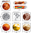 |
Fig. 1. Upper left panel: A brightness temperature (TB) map from ALMA’s Band 6 observation of the plage region at the start of the time series. The ellipse in the bottom left corner of the panel represents the beam size of the observations and the dashed white rectangle outlines the location of the long-lived fibril of interest. Upper right panel: Zoomed-in view of the selected fibril (using two different color tables for better clarity) with the seven artificial slits placed perpendicular to the fibril axis for wave analysis as discussed in Sect. 3. Middle and lower panels: Co-aligned SDO/HMI continuum and magnetogram and SDO/AIA images at 170, 30.4, 17.1, and 19.3 nm. In the SDO/HMI magnetogram, the line-of-sight photospheric magnetic fields (Blos) are in range of −1116 < Blos (G) < 81. |
3. Analysis and results
The ALMA Band 6 observations analyzed in this study present small-scale bright features throughout the plage region, along with a few extended, fibrillar dark structures on the left-hand side of the field of view (FoV) (see Fig. 1). Using the same dataset, Guevara Gómez et al. (2023) identified and detailed the properties of kink and sausage MHD wave modes in the small-scale bright structures. Field extrapolations of the photospheric magnetic fields from the Helioseismic and Magnetic Imager (HMI) presented by Schou et al. (2012); see Jafarzadeh et al. (2021), (Fig. 8) illustrate two main field topologies over the entire FoV: nearly vertical fields in the plage regions and nearly horizontal fields overarching a quiescent area (i.e., a neighboring internetwork region) in the areas covered by the extended and fibrillar dark structures.
In our Band 6 data, we do not observe many individual dark fibrils. Instead, we find a few extended dark structures, likely due to unresolved individual fibrils. However, we identified only one long-lived fibril (along with a few short-lived ones). Thus, we study here oscillatory signatures and their properties along the detected long-lived fibril.
3.1. Identification of oscillatory signals
To study waves and oscillations in the observed long-lived fibril, we tracked the dark elongated structure present in all frames, corresponding to a lifetime of 1568 s. We used the identification and tracking approach as previously introduced by Gafeira et al. (2017a,b). This method uses an unsharp mask algorithm and an adaptive histogram equalization procedure to enhance the intensity contrast between neighboring pixels and within the image (only for detection purposes). Using this method, we identified the long-lived fibril that persisted throughout the observed period. The spatial location of the fibril is marked by the dashed-line rectangle in the first frame of the time series, in the left panel of Fig. 1.
To quantify oscillatory signals along the fibril, we placed seven artificial slits perpendicular to the fibril axis, spaced 5 pixels apart (corresponding to 510 km on the solar disk). The upper right panel of Fig. 1 shows the fibril in the first frame, with the seven slits marked as vertical lines. The slits were positioned in the part of the fibril visible throughout the time series, as the fibril’s length varied over time. The lower panels of Fig. 1 show SDO/HMI continuum and magnetogram and SDO Atmospheric Imaging Assembly (AIA; Lemen et al. 2012) images at various wavelengths. We also examined Hα images from the Global Oscillation Network Group (GONG; Harvey et al. 2011); however, due to their relatively low spatial resolution, no corresponding features were visible within the ALMA FoV. While no clear counterpart was identified in the relatively low-resolution GONG Hα images, we anticipate correspondence with higher-resolution Hα observations. Molnar et al. (2019) found a strong correlation between ALMA 3 mm observations and the spatial structure of chromospheric features seen in high-resolution Hα line-core images. Based on their findings, we expect this fibril to have a corresponding counterpart visible in high-resolution Hα data. Similarly, we expect corresponding features to be present in extreme-ultraviolet (EUV) observations, particularly in AIA channels sensitive to transition region and coronal temperatures; although, high-resolution observations are necessary to resolve these relatively small structures. The co-aligned SDO/AIA images in the lower panel of Fig. 1 show that the fibril is located near a larger EUV loop (fibrillar structure) in the corona. That is less clear in the noisy 30.4 nm images. However, we note that larger-scale structures would likely show more similarities between ALMA and 30.4 nm images, as shown by Brajša et al. (2018) and Wedemeyer et al. (2020). Additionally, as is evident from the SDO images, the fibril lies above an internetwork region characterized by a magnetic canopy structure at chromospheric and coronal heights. Jafarzadeh et al. (2021), who calculated the approximate magnetic topology of these observations (from field extrapolations of the HMI observations), confirmed the predominantly horizontal magnetic field configuration in this region.
We measured the brightness temperature in all pixels along each slit and determined the fibril’s position at each location by finding the centroid of the slit using Gaussian fitting (representing the fibril’s horizontal displacement). Additionally, we calculated the brightness temperature at the centroid (representing the fibril’s intensity) and the full width at half maximum (FWHM) of the Gaussian fit (representing the fibril’s width) at each slit location.
3.2. Wavelet analysis
To characterize the wave properties of brightness temperature, width, and horizontal displacement, we performed a wavelet analysis. Wavelet analysis localizes spectral power in both time and frequency by decomposing the signal into time-localized wavelets, revealing how the frequency content of the signal changes over time (Daubechies 1990; Torrence & Compo 1998). We identified and removed the Cone of Influence (CoI), the unreliable areas in the time-frequency space subject to edge effects, from further analyses. We note that all signals (corresponding to brightness temperature, width, and horizontal displacement) were detrended by using a linear fit and then apodised using a Tukey window prior to the wavelet analyses. Furthermore, periods longer than 1000 s (i.e., less than 1 mHz) were subtracted from all signals by means of wavelet filtering. Such long periods are likely related to slow evolution of the magnetic structure, rather than wave signatures.
We calculated the wavelet power spectra of oscillations in all three parameters across the seven slits along the fibril using a Morlet function. This yielded the periods (or frequencies) of the fluctuations and their variations over time for each parameter. Additionally, we calculated the wavelet cross-power spectra between consecutive slits for each parameter, obtaining the phase relationships between the oscillations and, thus, the phase speeds of the waves propagating along the fibril.
Figure 2 illustrates examples of the wavelet power spectra. The left and middle columns show the power spectra of the oscillations of the three parameters at two consecutive slits (third and fourth slits) and the right column presents their corresponding wavelet cross-power spectra. The CoI regions are marked as cross-hatched areas and the black contours identify the 95% confidence levels. The arrows on the wavelet cross-power spectra indicate the relative phase relationship between oscillations in consecutive slits. Arrows pointing to the right represent in-phase oscillations (ϕ = 0°), arrows pointing to the left represent antiphase oscillations (ϕ = 180°), and arrows pointing down represent a 90° phase shift, where the second oscillation leads the first, indicating wave propagation from left to right along the fibril. In-phase and antiphase relationships are indicative of standing waves.
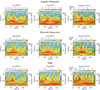 |
Fig. 2. Wavelet power spectra (left and middle columns) and wavelet cross-power spectra (right column) for oscillations in brightness temperature (top row), horizontal displacement (middle row), and width (bottom row) at two consecutive slits along the fibril. The cross-hatched areas indicate the wavelet’s cone of influence. In the cross-power spectra, arrows represent the phase relationship between oscillations at the two slits: rightward arrows indicate in-phase oscillations (0°), leftward arrows indicate antiphase oscillations (180°), and downward arrows indicate the second slit leading the first by 90°. Black contours in all panels mark the 95% confidence level. |
As shown in the right column of Fig. 2, all three parameters (brightness temperature, horizontal displacement, and width) exhibit a combination of standing and propagating waves. The normalized phase-lag distributions (Fig. 3) reveal a dominance of in-phase and antiphase relationships, particularly for brightness temperature and horizontal displacement, suggesting a prevalence of standing waves. However, the presence of numerous other phase values indicates that propagating waves are also present. We note that some of the abrupt changes in phase angles could be due to noise or spurious signals.
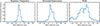 |
Fig. 3. Normalized distributions of phase differences between oscillations in brightness temperature (left), horizontal displacement (middle), and width (right) at pairs of consecutive slits along the fibril. |
We also calculated the wavelet cross-power spectra between pairs of parameters (brightness temperature and horizontal displacement, brightness temperature and width, and horizontal displacement and width) at each slit to determine the phase correlation of oscillations within the same slit. However, interpreting such relationships is complex due to the potential superposition of multiple MHD wave modes, which current theoretical models are not yet sophisticated enough to fully disentangle, as discussed by Jafarzadeh et al. (2024). A preliminary analysis suggested that brightness temperature and horizontal displacement oscillations primarily exhibited in-phase and antiphase relationships, while brightness temperature and width oscillations showed a more isotropic distribution of phase differences with slight peaks at 0° and ±180°. Horizontal displacement and width oscillations displayed diverse phase angles, but in-phase and antiphase relationships still dominate, though less strongly than for brightness temperature and horizontal displacement.
3.2.1. Wave periods
Figure 4 presents the normalized distributions of the wave periods for brightness temperature, horizontal displacement, and width along the fibril. These distributions were constructed by considering all power-weighted periods within the 95% confidence levels and outside the CoI of the wavelet cross-power spectra calculated for each slit. The final distribution was then normalized by its maximum value to facilitate comparison.
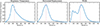 |
Fig. 4. Normalized distributions of oscillation periods in brightness temperature, horizontal displacement, and width derived from wavelet cross-power spectra. The vertical dashed lines identify the median of each distribution. |
The distributions for all three parameters exhibit a broad range of periods, extending from approximately 15 to 700 s. The brightness-temperature and horizontal-displacement histograms display single-peak distributions with distinct peaks at 200 and 225 s, respectively. The width distribution shows a primary peak at 300 s and two less pronounced peaks around 80 and 150 s. Table 1 summarizes the range, mean, median, and standard deviation of the oscillation periods for each parameter, as determined from the wavelet analysis.
Properties of oscillation periods from the wavelet analysis.
3.2.2. Phase speeds
The phase lag between two points in a traveling wave represents how much one wave has advanced relative to the other, directly translating to a travel time between those points. In a standing wave, a ±180° phase-lag signifies a special relationship of persistent antiphase oscillation, rather than a measure of propagation. However, standing waves can result from the superposition (interference) of two waves traveling in opposite directions, each with its own phase speed.
To quantify wave propagation, we calculated the propagation time (τ) between pairs of consecutive slits along the fibril, using the following:
 (1)
(1)
where ϕ is the phase angle (excluding ±180°) and P is the wave period, with both being obtained from the wavelet analysis. In this calculation, we also considered only phase differences that fall within the 95% confidence levels and outside the CoI of the wavelet cross-power spectra. These phase differences are further weighted by power, emphasizing the significance of correlation strengths in the time-frequency domain.
Knowing the fixed distance between slits (510 km) and the calculated time lags, we determined the phase speed (or propagation speed) for brightness temperature, width, and horizontal displacement oscillations. Figure 5 shows distributions of the absolute values of phase velocities, which include both leftward-propagating and rightward-propagating waves. The coexistence of these oppositely propagating waves in the same structure may suggest that at least some of the observed standing wave patterns (those with 0° phase lags) may result from their superposition. Table 2 summarizes the mean, median, and standard deviation of the propagation speeds, along with the occurrence rates of leftward and rightward propagation.
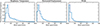 |
Fig. 5. Normalized distributions of absolute phase speeds for oscillations in brightness temperature, horizontal displacement, and width along the fibril. The vertical dashed lines mark the median of each distribution. |
Properties of phase speeds from the wavelet analysis.
4. Discussion and conclusions
Using high-cadence (2 s) ALMA Band 6 observations, we investigated the presence of MHD waves in a long-lasting (≈1600 s) dark fibrillar structure, which represent strong magnetic field bundles in the upper chromosphere. By placing multiple, equally spaced (510 km), artificial slits perpendicular to the fibril axis, we examined oscillations in brightness temperature, horizontal displacement, and width along the length of each slit.
Our analysis revealed a combination of both standing and propagating waves in all three parameters, with oscillation periods ranging from approximately 15 to 700 s. The period distributions of brightness temperature and horizontal displacement exhibited single-peaked histograms, with median and standard deviations of 240 ± 114 s, 225 ± 102 s, respectively. The width distribution showed a primary peak at 300 s and two less pronounced secondary peaks around 80 and 150 s, with a period of 272 ± 118 s as the median and standard deviation of the distribution.
The propagating waves exhibited mean absolute phase velocities (with a median and standard deviation) of 74 ± 204 km/s for brightness temperature, 52 ± 197 km/s for horizontal displacement, and 28 ± 254 km/s for width. The transverse oscillations likely represent the presence of MHD kink modes (Spruit 1982), while the size fluctuations (width oscillations) likely indicate sausage modes (Roberts 1981; Moreels et al. 2013).
Our findings are consistent with previous studies of MHD waves in chromospheric structures observed with ALMA. Guevara Gómez et al. (2021) reported a similar oscillatory behavior in bright point-like features, identifying fast sausage modes with average oscillation periods of 90 ± 22 s for brightness temperature and 110 ± 12 s for size. These periods are shorter than those found in our dark fibril, potentially due to variations in the magnetic field strength and geometry between the two types of structures.
Subsequent studies using ALMA have also focused on small-scale bright features, interpreted as cross sections of magnetic flux tubes (manifesting as fibrils when oriented horizontally). Guevara Gómez et al. (2022) detailed the propagation of transverse kink waves in these structures using ALMA sub-bands, while Guevara Gómez et al. (2023) analyzed MHD wave modes in a larger sample. They found evidence of transverse (kink) waves with average amplitude velocities of 2−4.3 km/s and compressible sausage modes, with average oscillation periods of 70−110 s for brightness temperature, 61−100 s for size, and 57−80 s for horizontal velocity. These values of periods and velocities are smaller than those observed in our dark fibril, likely because these small bright features form at lower atmospheric heights.
Comparing with studies of MHD waves in fibrillar structures observed in other diagnostics, both kink and sausage modes were detected in bright slender Ca II H fibrils (located in the low-to-mid chromosphere) from high-resolution SUNRISE observations (Solanki et al. 2017), with periods on the order of 83 and 35 s, and phase speeds of 9 ± 14 and 11−15 km/s, respectively (Jafarzadeh et al. 2017a; Gafeira et al. 2017a). Longer periods (232 and 197 s) and larger propagating speeds (80 and 67 km/s) were reported by Morton et al. (2012) for higher chromospheric (dark) fibrillar structures, comparable with those we found in the present work.
While relatively short periods (shorter than, e.g., 100 s) have been more frequently observed in the low chromosphere, they are less common in the upper chromosphere (see also, De Pontieu et al. 2007a; Pietarila et al. 2011; Kuridze et al. 2012; Morton et al. 2013, 2014, 2021), where our ALMA fibril is likely located (Chintzoglou et al. 2021b). Such short-period waves could possibly be dissipated through the chromospheric heights before reaching the upper layers.
Leveraging both observational data and numerical simulations, Jess et al. (2012) suggested that mode conversions in the lower solar atmosphere can be a main driver of the MHD kink and sausage modes observed in chromospheric fibrillar structures (in on-disk Type I spicules). This mechanism could also play a role in the excitation of the waves we observe in the upper chromospheric fibril.
Theoretical studies have shown that asymmetry in waveguides, such as the dark fibril studied here, can influence MHD wave properties, including the coupling of different wave modes, shifts in phase speeds, and modifications in damping rates (Allcock & Erdélyi 2017, 2018; Erdélyi & Zsámberger 2024). Furthermore, irregularities within these waveguides can significantly alter the properties and characteristics of resonant modes, particularly those of higher MHD wave modes (Albidah et al. 2021, 2022). While our current analysis primarily focuses on identifying kink and sausage modes, future investigations incorporating the effects of waveguide asymmetry could offer deeper insights into these effects and their implications for the wave dynamics observed in these dark fibrils. Such studies would require detailed modeling of the fibril’s cross-sectional shape and density structure, which could be achieved by combining high-resolution observations with advanced MHD wave modeling techniques.
In conclusion, our study provides the first piece of evidence for the ubiquitous presence of MHD waves in dark fibrils observed by ALMA in Band 6. The detection of both standing and propagating waves, alongside the identification of potential kink and sausage modes, underscores the complex wave dynamics within these structures. The distinct wave properties observed here, compared to other chromospheric features, highlight the importance of considering factors such as magnetic field strength and geometry when interpreting wave phenomena. Importantly, this work demonstrates ALMA’s capability to effectively sample such dynamic dark fibrillar structures, despite previous doubts. Future statistical studies of these fibrils using higher-resolution ALMA observations across multiple bands promise to further enhance our understanding of MHD wave behavior in the chromosphere.
Acknowledgments
This work is supported by the SolarALMA project, which received funding from the European Research Council (ERC) under the European Union’s Horizon 2020 research and innovation program (grant agreement No. 682462), and by the ESGC project (project No. 335497) funded by the the Research Council of Norway, and by the Research Council of Norway through its Centres of Excellence scheme, project number 262622. S.J. gratefully acknowledges support from the Rosseland Center for Solar Physics (RoCS), University of Oslo, Norway. D.B.J. acknowledges support from the Leverhulme Trust via the Research Project Grant RPG-2019-371, as well as the UK Space Agency via the National Space Technology Programme (grant SSc-009). D.B.J. also wishes to thank the UK Science and Technology Facilities Council (STFC) for the consolidated grants ST/T00021X/1 and ST/X000923/1. R.G. acknowledges the support by Fundação para a Ciência e a Tecnologia (FCT) through the research grants UIDB/04434/2020 and UIDP/04434/2020. This paper makes use of the following ALMA data: ADS/JAO.ALMA#2016.1.00050.S. ALMA is a partnership of ESO (representing its member states), NSF (USA) and NINS (Japan), together with NRC (Canada), MOST and ASIAA (Taiwan), and KASI (Republic of Korea), in cooperation with the Republic of Chile. The Joint ALMA Observatory is operated by ESO, AUI/NRAO and NAOJ. We are grateful to the many colleagues who contributed to developing the Solar observing modes for ALMA and for support from the ALMA regional centres. We wish to acknowledge scientific discussions with the Waves in the Lower Solar Atmosphere (WaLSA; https://WaLSA.team) team, which has been supported by the Research Council of Norway (project no. 262622), The Royal Society (award no. Hooke18b/SCTM; Jess et al. 2021), and the International Space Science Institute (ISSI Team 502).
References
- Albidah, A. B., Brevis, W., Fedun, V., et al. 2021, Philos. Trans. R. Soc. London Ser. A, 379, 20200181 [Google Scholar]
- Albidah, A. B., Fedun, V., Aldhafeeri, A. A., et al. 2022, ApJ, 927, 201 [NASA ADS] [CrossRef] [Google Scholar]
- Allcock, M., & Erdélyi, R. 2017, Sol. Phys., 292, 35 [NASA ADS] [CrossRef] [Google Scholar]
- Allcock, M., & Erdélyi, R. 2018, ApJ, 855, 90 [NASA ADS] [CrossRef] [Google Scholar]
- Baker, D., Stangalini, M., Valori, G., et al. 2021, ApJ, 907, 16 [Google Scholar]
- Bate, W., Jess, D. B., Nakariakov, V. M., et al. 2022, ApJ, 930, 129 [NASA ADS] [CrossRef] [Google Scholar]
- Bate, W., Jess, D. B., Grant, S. D. T., et al. 2024, ApJ, 970, 66 [NASA ADS] [CrossRef] [Google Scholar]
- Bogdan, T. J., Carlsson, M., Hansteen, V. H., et al. 2003, ApJ, 599, 626 [Google Scholar]
- Brajša, R., Sudar, D., Benz, A. O., et al. 2018, A&A, 613, A17 [NASA ADS] [CrossRef] [EDP Sciences] [Google Scholar]
- Brajša, R., Skokić, I., Sudar, D., et al. 2021, A&A, 651, A6 [NASA ADS] [CrossRef] [EDP Sciences] [Google Scholar]
- Brooks, D. H., Ugarte-Urra, I., & Warren, H. P. 2015, Nat. Commun., 6, 5947 [Google Scholar]
- Chai, Y., Gary, D. E., Reardon, K. P., & Yurchyshyn, V. 2022, ApJ, 924, 100 [NASA ADS] [CrossRef] [Google Scholar]
- Chintzoglou, G., De Pontieu, B., Martínez-Sykora, J., et al. 2021a, ApJ, 906, 83 [NASA ADS] [CrossRef] [Google Scholar]
- Chintzoglou, G., De Pontieu, B., Martínez-Sykora, J., et al. 2021b, ApJ, 906, 82 [CrossRef] [Google Scholar]
- Choudhuri, A. R., Auffret, H., & Priest, E. R. 1993, Sol. Phys., 143, 49 [NASA ADS] [CrossRef] [Google Scholar]
- da Silva Santos, J. M., de la Cruz Rodríguez, J., White, S. M., et al. 2020a, A&A, 643, A41 [EDP Sciences] [Google Scholar]
- da Silva Santos, J. M., de la Cruz Rodríguez, J., Leenaarts, J., et al. 2020b, A&A, 634, A56 [NASA ADS] [CrossRef] [EDP Sciences] [Google Scholar]
- Daubechies, I. 1990, IEEE Trans. Inf. Theor., 36, 961 [Google Scholar]
- De Pontieu, B., Hansteen, V. H., Rouppe van der Voort, L., van Noort, M., & Carlsson, M. 2007a, ApJ, 655, 624 [Google Scholar]
- De Pontieu, B., McIntosh, S. W., Carlsson, M., et al. 2007b, Science, 318, 1574 [Google Scholar]
- De Pontieu, B., Title, A. M., Lemen, J. R., et al. 2014, Sol. Phys., 289, 2733 [Google Scholar]
- Edwin, P. M., & Roberts, B. 1983, Sol. Phys., 88, 179 [Google Scholar]
- Eklund, H., Wedemeyer, S., Szydlarski, M., Jafarzadeh, S., & Guevara Gómez, J. C. 2020, A&A, 644, A152 [NASA ADS] [CrossRef] [EDP Sciences] [Google Scholar]
- Eklund, H., Wedemeyer, S., Szydlarski, M., & Jafarzadeh, S. 2021a, A&A, 656, A68 [NASA ADS] [CrossRef] [EDP Sciences] [Google Scholar]
- Eklund, H., Wedemeyer, S., Snow, B., et al. 2021b, Philos. Trans. R. Soc. London Ser. A, 379, 20200185 [NASA ADS] [Google Scholar]
- Erdélyi, R., & Zsámberger, N. K. 2024, Symmetry, 16, 1228 [Google Scholar]
- Gabriel, A. H. 1976, Philos. Trans. R. Soc. London Ser. A, 281, 339 [NASA ADS] [CrossRef] [Google Scholar]
- Gafeira, R., Jafarzadeh, S., Solanki, S. K., et al. 2017a, ApJS, 229, 7 [Google Scholar]
- Gafeira, R., Lagg, A., Solanki, S. K., et al. 2017b, ApJS, 229, 6 [NASA ADS] [CrossRef] [Google Scholar]
- Gilchrist-Millar, C. A., Jess, D. B., Grant, S. D. T., et al. 2021, Philos. Trans. R. Soc. London Ser. A, 379, 20200172 [Google Scholar]
- Giovanelli, R. G., & Jones, H. P. 1982, Sol. Phys., 79, 267 [NASA ADS] [CrossRef] [Google Scholar]
- Grant, S. D. T., Jess, D. B., Moreels, M. G., et al. 2015, ApJ, 806, 132 [Google Scholar]
- Grant, S. D. T., Jess, D. B., Zaqarashvili, T. V., et al. 2018, Nat. Phys., 14, 480 [Google Scholar]
- Guevara Gómez, J. C., Jafarzadeh, S., Wedemeyer, S., et al. 2021, Philos. Trans. R. Soc. A., 379, 20200184 [Google Scholar]
- Guevara Gómez, J. C., Jafarzadeh, S., Wedemeyer, S., & Szydlarski, M. 2022, A&A, 665, L2 [NASA ADS] [CrossRef] [EDP Sciences] [Google Scholar]
- Guevara Gómez, J. C., Jafarzadeh, S., Wedemeyer, S., et al. 2023, A&A, 671, A69 [NASA ADS] [CrossRef] [EDP Sciences] [Google Scholar]
- Harvey, J. W., Bolding, J., Clark, R., et al. 2011, AAS/Solar Physics Division Meeting, 42, 17.45 [NASA ADS] [Google Scholar]
- He, J., Marsch, E., Tu, C., & Tian, H. 2009, ApJ, 705, L217 [NASA ADS] [CrossRef] [Google Scholar]
- Henriques, V. M. J., Jafarzadeh, S., Guevara Gómez, J. C., et al. 2022, A&A, 659, A31 [NASA ADS] [CrossRef] [EDP Sciences] [Google Scholar]
- Houston, S. J., Jess, D. B., Keppens, R., et al. 2020, ApJ, 892, 49 [NASA ADS] [CrossRef] [Google Scholar]
- Jafarzadeh, S., Solanki, S. K., Gafeira, R., et al. 2017a, ApJS, 229, 9 [Google Scholar]
- Jafarzadeh, S., Rutten, R. J., Solanki, S. K., et al. 2017b, ApJS, 229, 11 [CrossRef] [Google Scholar]
- Jafarzadeh, S., Wedemeyer, S., Szydlarski, M., et al. 2019, A&A, 622, A150 [NASA ADS] [CrossRef] [EDP Sciences] [Google Scholar]
- Jafarzadeh, S., Wedemeyer, S., Fleck, B., et al. 2021, Philos. Trans. R. Soc. London Ser. A, 379, 20200174 [NASA ADS] [Google Scholar]
- Jafarzadeh, S., Schiavo, L. A. C. A., Fedun, V., et al. 2024, A&A, 688, A2 [NASA ADS] [CrossRef] [EDP Sciences] [Google Scholar]
- Jess, D. B., Pascoe, D. J., Christian, D. J., et al. 2012, ApJ, 744, L5 [NASA ADS] [CrossRef] [Google Scholar]
- Jess, D. B., Morton, R. J., Verth, G., et al. 2015, Space Sci. Rev., 190, 103 [Google Scholar]
- Jess, D. B., Keys, P. H., Stangalini, M., & Jafarzadeh, S. 2021, Philos. Trans. R. Soc. London Ser. A, 379, 20200169 [Google Scholar]
- Jess, D. B., Jafarzadeh, S., Keys, P. H., et al. 2023, Liv. Rev. Sol. Phys., 20, 1 [NASA ADS] [CrossRef] [Google Scholar]
- Kuridze, D., Morton, R. J., Erdélyi, R., et al. 2012, ApJ, 750, 51 [NASA ADS] [CrossRef] [Google Scholar]
- Leer, E., Holzer, T. E., & Fla, T. 1982, Space Sci. Rev., 33, 161 [Google Scholar]
- Lemen, J. R., Title, A. M., Akin, D. J., et al. 2012, Sol. Phys., 275, 17 [Google Scholar]
- Loukitcheva, M. 2019, Adv. Space Res., 63, 1396 [Google Scholar]
- McIntosh, S. W., de Pontieu, B., Carlsson, M., et al. 2011, Nature, 475, 477 [Google Scholar]
- Molnar, M. E., Reardon, K. P., Chai, Y., et al. 2019, ApJ, 881, 99 [Google Scholar]
- Moreels, M. G., Goossens, M., & Van Doorsselaere, T. 2013, A&A, 555, A75 [NASA ADS] [CrossRef] [EDP Sciences] [Google Scholar]
- Morton, R. J., Verth, G., Jess, D. B., et al. 2012, Nat. Commun., 3, 1315 [Google Scholar]
- Morton, R. J., Verth, G., Fedun, V., Shelyag, S., & Erdélyi, R. 2013, ApJ, 768, 17 [Google Scholar]
- Morton, R. J., Verth, G., Hillier, A., & Erdélyi, R. 2014, ApJ, 784, 29 [NASA ADS] [CrossRef] [Google Scholar]
- Morton, R. J., Mooroogen, K., & Henriques, V. M. J. 2021, Philos. Trans. R. Soc. London Ser. A, 379, 20200183 [NASA ADS] [Google Scholar]
- Murabito, M., Stangalini, M., Baker, D., et al. 2021, A&A, 656, A87 [NASA ADS] [CrossRef] [EDP Sciences] [Google Scholar]
- Murabito, M., Stangalini, M., Laming, J. M., et al. 2024, Phys. Rev. Lett., 132, 215201 [CrossRef] [Google Scholar]
- Musielak, Z. E., & Ulmschneider, P. 2003, A&A, 406, 725 [NASA ADS] [CrossRef] [EDP Sciences] [Google Scholar]
- Narang, N., Chandrashekhar, K., Jafarzadeh, S., et al. 2022, A&A, 661, A95 [NASA ADS] [CrossRef] [EDP Sciences] [Google Scholar]
- Nindos, A., Alissandrakis, C. E., Patsourakos, S., & Bastian, T. S. 2020, A&A, 638, A62 [NASA ADS] [CrossRef] [EDP Sciences] [Google Scholar]
- Nindos, A., Patsourakos, S., Alissandrakis, C. E., & Bastian, T. S. 2021, A&A, 652, A92 [NASA ADS] [CrossRef] [EDP Sciences] [Google Scholar]
- Nindos, A., Patsourakos, S., Jafarzadeh, S., & Shimojo, M. 2022, Front. Astron. Space Sci., 9, 981205 [Google Scholar]
- Nutto, C., Steiner, O., Schaffenberger, W., & Roth, M. 2012, A&A, 538, A79 [NASA ADS] [CrossRef] [EDP Sciences] [Google Scholar]
- Patsourakos, S., Alissandrakis, C. E., Nindos, A., & Bastian, T. S. 2020, A&A, 634, A86 [NASA ADS] [CrossRef] [EDP Sciences] [Google Scholar]
- Pesnell, W. D., Thompson, B. J., & Chamberlin, P. C. 2012, Sol. Phys., 275, 3 [Google Scholar]
- Pietarila, A., Aznar Cuadrado, R., Hirzberger, J., & Solanki, S. K. 2011, ApJ, 739, 92 [NASA ADS] [CrossRef] [Google Scholar]
- Riedl, J. M., Gilchrist-Millar, C. A., Van Doorsselaere, T., Jess, D. B., & Grant, S. D. T. 2021, A&A, 648, A77 [NASA ADS] [CrossRef] [EDP Sciences] [Google Scholar]
- Roberts, B. 1981, Sol. Phys., 69, 39 [NASA ADS] [CrossRef] [Google Scholar]
- Rouppe van der Voort, L., Leenaarts, J., De Pontieu, B., Carlsson, M., & Vissers, G. 2009, ApJ, 705, 272 [Google Scholar]
- Rutten, R. J. 2017, A&A, 598, A89 [NASA ADS] [CrossRef] [EDP Sciences] [Google Scholar]
- Schou, J., Scherrer, P. H., Bush, R. I., et al. 2012, Sol. Phys., 275, 229 [Google Scholar]
- Shimojo, M., Bastian, T. S., Hales, A. S., et al. 2017, Sol. Phys., 292, 87 [Google Scholar]
- Solanki, S. K. 1993, Space Sci. Rev., 63, 1 [Google Scholar]
- Solanki, S. K., Steiner, O., & Uitenbroeck, H. 1991, A&A, 250, 220 [NASA ADS] [Google Scholar]
- Solanki, S. K., Riethmüller, T. L., Barthol, P., et al. 2017, ApJS, 229, 2 [NASA ADS] [CrossRef] [Google Scholar]
- Spruit, H. C. 1982, Sol. Phys., 75, 3 [Google Scholar]
- Stangalini, M., Del Moro, D., Berrilli, F., & Jefferies, S. M. 2011, A&A, 534, A65 [NASA ADS] [CrossRef] [EDP Sciences] [Google Scholar]
- Stangalini, M., Baker, D., Valori, G., et al. 2021, Philos. Trans. R. Soc. London Ser. A, 379, 20200216 [NASA ADS] [Google Scholar]
- Torrence, C., & Compo, G. P. 1998, Bull. Am. Meteorol. Soc., 79, 61 [Google Scholar]
- Ulmschneider, P., Priest, E. R., & Rosner, R. 1991, Mechanisms of Chromospheric and Coronal Heating (Berlin: Springer-Verlag) [CrossRef] [Google Scholar]
- Verth, G., & Jess, D. B. 2016, Washington DC American Geophysical Union Geophysical Monograph Series, 216, 431 [Google Scholar]
- Wedemeyer, S., Bastian, T., Brajša, R., et al. 2016, Space Sci. Rev., 200, 1 [Google Scholar]
- Wedemeyer, S., Szydlarski, M., Jafarzadeh, S., et al. 2020, A&A, 635, A71 [NASA ADS] [CrossRef] [EDP Sciences] [Google Scholar]
- Wedemeyer-Böhm, S., Lagg, A., & Nordlund, Å. 2009, Space Sci. Rev., 144, 317 [Google Scholar]
- White, S. M., Iwai, K., Phillips, N. M., et al. 2017, Sol. Phys., 292, 88 [Google Scholar]
- Wootten, A., & Thompson, A. R. 2009, IEEE Proc., 97, 1463 [NASA ADS] [CrossRef] [Google Scholar]
All Tables
All Figures
|
Fig. 1. Upper left panel: A brightness temperature (TB) map from ALMA’s Band 6 observation of the plage region at the start of the time series. The ellipse in the bottom left corner of the panel represents the beam size of the observations and the dashed white rectangle outlines the location of the long-lived fibril of interest. Upper right panel: Zoomed-in view of the selected fibril (using two different color tables for better clarity) with the seven artificial slits placed perpendicular to the fibril axis for wave analysis as discussed in Sect. 3. Middle and lower panels: Co-aligned SDO/HMI continuum and magnetogram and SDO/AIA images at 170, 30.4, 17.1, and 19.3 nm. In the SDO/HMI magnetogram, the line-of-sight photospheric magnetic fields (Blos) are in range of −1116 < Blos (G) < 81. |
| In the text | |
|
Fig. 2. Wavelet power spectra (left and middle columns) and wavelet cross-power spectra (right column) for oscillations in brightness temperature (top row), horizontal displacement (middle row), and width (bottom row) at two consecutive slits along the fibril. The cross-hatched areas indicate the wavelet’s cone of influence. In the cross-power spectra, arrows represent the phase relationship between oscillations at the two slits: rightward arrows indicate in-phase oscillations (0°), leftward arrows indicate antiphase oscillations (180°), and downward arrows indicate the second slit leading the first by 90°. Black contours in all panels mark the 95% confidence level. |
| In the text | |
|
Fig. 3. Normalized distributions of phase differences between oscillations in brightness temperature (left), horizontal displacement (middle), and width (right) at pairs of consecutive slits along the fibril. |
| In the text | |
|
Fig. 4. Normalized distributions of oscillation periods in brightness temperature, horizontal displacement, and width derived from wavelet cross-power spectra. The vertical dashed lines identify the median of each distribution. |
| In the text | |
|
Fig. 5. Normalized distributions of absolute phase speeds for oscillations in brightness temperature, horizontal displacement, and width along the fibril. The vertical dashed lines mark the median of each distribution. |
| In the text | |
Current usage metrics show cumulative count of Article Views (full-text article views including HTML views, PDF and ePub downloads, according to the available data) and Abstracts Views on Vision4Press platform.
Data correspond to usage on the plateform after 2015. The current usage metrics is available 48-96 hours after online publication and is updated daily on week days.
Initial download of the metrics may take a while.