| Issue |
A&A
Volume 662, June 2022
|
|
|---|---|---|
| Article Number | A88 | |
| Number of page(s) | 15 | |
| Section | The Sun and the Heliosphere | |
| DOI | https://doi.org/10.1051/0004-6361/202142087 | |
| Published online | 21 June 2022 | |
Active region chromospheric magnetic fields
Observational inference versus magnetohydrostatic modelling
1
Institute for Solar Physics, Department of Astronomy, Stockholm University, AlbaNova University Centre, 106 91 Stockholm, Sweden
e-mail: This email address is being protected from spambots. You need JavaScript enabled to view it.
2
CAS Key Laboratory of Solar Activity, National Astronomical Observatories, Chinese Academy of Sciences, Beijing, PR China
3
Max Planck Institute for Solar System Research, Justus-von-Liebig-Weg 3, 37077 Göttingen, Germany
Received:
25
August
2021
Accepted:
27
April
2022
Abstract
Context. A proper estimate of the chromospheric magnetic fields is thought to improve modelling of both active region and coronal mass ejection evolution. However, because the chromospheric field is not regularly obtained for sufficiently large fields of view, estimates thereof are commonly obtained through data-driven models or field extrapolations, based on photospheric boundary conditions alone and involving pre-processing that may reduce details and dynamic range in the magnetograms.
Aims. We investigate the similarity between the chromospheric magnetic field that is directly inferred from observations and the field obtained from a magnetohydrostatic (MHS) extrapolation based on a high-resolution photospheric magnetogram.
Methods. Based on Swedish 1-m Solar Telescope Fe I 6173 Å and Ca II 8542 Å observations of NOAA active region 12723, we employed the spatially regularised weak-field approximation (WFA) to derive the vector magnetic field in the chromosphere from Ca II, as well as non-local thermodynamic equilibrium (non-LTE) inversions of Fe I and Ca II to infer a model atmosphere for selected regions. Milne-Eddington inversions of Fe I serve as photospheric boundary conditions for the MHS model that delivers the three-dimensional field, gas pressure, and density self-consistently.
Results. For the line-of-sight component, the MHS chromospheric field generally agrees with the non-LTE inversions and WFA, but tends to be weaker by 16% on average than these when larger in magnitude than 300 G. The observationally inferred transverse component is systematically stronger, up to an order of magnitude in magnetically weaker regions, but the qualitative distribution with height is similar to the MHS results. For either field component, the MHS chromospheric field lacks the fine structure derived from the inversions. Furthermore, the MHS model does not recover the magnetic imprint from a set of high fibrils connecting the main polarities.
Conclusions. The MHS extrapolation and WFA provide a qualitatively similar chromospheric field, where the azimuth of the former is better aligned with Ca II 8542 Å fibrils than that of the WFA, especially outside strong-field concentrations. The amount of structure as well as the transverse field strengths are, however, underestimated by the MHS extrapolation. This underscores the importance of considering a chromospheric magnetic field constraint in data-driven modelling of active regions, particularly in the context of space weather predictions.
Key words: Sun: activity / Sun: chromosphere / Sun: photosphere / Sun: magnetic fields / radiative transfer
© G. J. M. Vissers et al. 2022
 Open Access article, published by EDP Sciences, under the terms of the Creative Commons Attribution License (https://creativecommons.org/licenses/by/4.0), which permits unrestricted use, distribution, and reproduction in any medium, provided the original work is properly cited.
This article is published in open access under the Subscribe-to-Open model. This email address is being protected from spambots. You need JavaScript enabled to view it. to support open access publication.
1. Introduction
Our monitoring capabilities of solar activity drastically improved with the constant coverage from the photosphere to the corona that the Solar Dynamics Observatory (SDO; Pesnell et al. 2012) and its two instruments, the Atmospheric Imaging Assembly (AIA; Lemen et al. 2012) and Helioseismic and Magnetic Imager (HMI; Scherrer et al. 2012; Schou et al. 2012), afford since early 2010. SDO/HMI provides full-disk photospheric vector-magnetograms that have been used as the basis for field extrapolations and bottom boundary conditions in data-driven modelling of flare-productive active regions (e.g., Jin et al. 2016; Price et al. 2020), for instance. Similar observations are not currently obtained on a routine basis for the chromospheric magnetic field1, while several studies indicate that including the chromospheric field vector is benificial both for data-driven modelling and recovering chromospheric and coronal magnetic field structures in extrapolations (e.g., De Rosa et al. 2009; Fleishman et al. 2019; Toriumi et al. 2020). A chromospheric field constraint on erupting flux ropes could also aid in modelling and forecasting the evolution of coronal mass ejections (CMEs), thereby likely improving the predictions for the geo-effectiveness of CMEs (Kilpua et al. 2019).
In the absence of chromospheric constraints, data-driven modelling relies on magnetic (and electric) field boundary conditions from the photosphere alone (but see Metcalf et al. 2008; Wiegelmann et al. 2008). Depending on the modelling approach, the HMI magnetograms are passed through several pre-processing steps that serve avoid flux-imbalance and nudge the bottom boundary to a force-free state or ensure numerical stability, for example, but these may also impact the modelled field configuration in the higher atmosphere. For instance, Vissers et al. (2021), analysing the X2.2 flare of 2017-09-06T09:10 in AR 12673, reported discrepancies that can in part be attributed to the pre-processing that smoothes and modifies the photospheric field, but they also pointed out the importance of higher resolution in the modelling to uncover details in the chromospheric atmospheric field configuration. Both likely affect the photospheric and chromospheric field estimates and may thus have implications for the space weather modelling that builds on such data-driven models. The magnetohydrostatic (MHS) model (Zhu & Wiegelmann 2018, 2019; Zhu et al. 2020) that we consider here includes part of the aforementioned pre-processing, but uses the original photospheric magnetogram as bottom boundary condition while iteratively reaching a solution, which could yield a better estimate of the chromospheric field configuration.
With current instrumentation, the field of view (FOV) for high-resolution chromospheric observations is often constrained to some 50″–70″ on the side, meaning that larger active regions (or flux ropes, for that matter) cannot typically be contained entirely within a single pointing, thereby limiting the benefits from incorporating such observations as boundary conditions for modelling larger-scale structures. A solution to this is to canvas extended regions by mosaicking (e.g., Reardon & Cauzzi 2012; Hammerschlag et al. 2013), but such observations have not been common practice at the Swedish 1-m Solar Telescope (SST; Scharmer et al. 2003). Indeed, only one such study exists (Scullion et al. 2014), presenting a 9 × 6 mosaic that covers an active region with a FOV of 280″ × 180 in Hα imaging spectroscopy. However, recent improvements in the SST pointing control software have now rendered mosaicking a relatively simple task.
Here we analyse a flux-balanced mosaic of NOAA active region (AR) 12723 and compare its chromospheric magnetic field as inferred from the observations with that from an MHS model based on a high-resolution photospheric vector magnetogram. A spatially regularised weak-field approximation (WFA) delivers the full-FOV chromospheric magnetic field, while we use Milne-Eddington (ME) inversions to obtain the photospheric field vector, which also serves as boundary condition for the MHS extrapolation model. Furthermore, we perform non-local thermodynamic equilibrium (non-LTE) inversions of selected regions of interest (ROIs) to allow a depth-stratified comparison with the MHS model.
The remainder of this publication is structured as follows. Section 2 introduces the observations, mosaic construction, and post-processing to prepare the data for inversions. Section 3 describes the ME, WFA, and non-LTE inversion techniques used to infer the photospheric and chromospheric magnetic field vectors, as well as the MHS model setup. We present our results in Sect. 4, considering the field vector both for several regions of interest and on larger, active region scales. Finally, we discuss our findings in Sect. 5 and present our conclusions in Sect. 6.
2. Observations and reduction
On 2018-09-30, we observed NOAA AR 12723 with the CRisp Imaging SpectroPolarimeter (CRISP; Scharmer et al. 2008) and CHROMIS (Scharmer 2017) at the SST. These observations consist of two rounds of four overlapping pointings in a 2 × 2 pattern for a context mosaic, followed by a regular, single-pointing time series. For this study, we focus only on the context data and selected the set of pointings with the highest image contrast to construct the mosaic that we analyse here.
The mosaic has a mean observing time of 09:24:03 UT, is centred at (X, Y) = (95″, −270″), corresponding to μ = 0.95, and covers about 110″ × 110 at 0 058 pix−1. Figure 1 presents the mosaic in Ca II (in helioprojective representation), with photospheric and chromospheric vertical magnetic field maps and context magnetic field from an SDO HMI active region patch (SHARP; Bobra et al. 2014) in cylindrical equal-area (CEA) projection.
 |
Fig. 1. SST/CRISP mosaic and context SDO/HMI-derived SHARP magnetic field of NOAA AR 12723. Upper left: Ca II 8542 Å line core image. Upper right: Milne-Eddington inferred photospheric Br magnetic field from Fe I 6173 Å observations by SST/CRISP. Lower left: chromospheric radial magnetic field Br from the spatially regularised WFA. Lower right: same as the upper right panel, but from SDO/HMI. The line-of-sight magnetic field maps have been clipped to ±1.5 kG and are all reprojected and mapped to cylindrical equal-area (CEA) coordinates. The mapping to CEA precludes any direct comparison by coordinate of features in the top left panel vs. the other panels. The white boxes in the top left panel indicate narrow regions of interest (ROIs) selected for (non-)LTE inversion and are indicated (approximately, i.e. without mapping distortion) by cyan boxes in the top right and bottom left panels. The dashed green box in the top right panel highlights the FOV selected for the magnetohydrostatic simulation, while the purple contour in the lower right panel traces the SST mosaic field of view. |
Imaging spectropolarimetry was obtained in the Fe I 6173 Å and Ca II 8542 Å lines. Fe I was sampled at eight different wavelengths, equidistantly distributed at 40 mÅ spacing between −0.12 Å and +0.16 Å. The Ca II sampling covers ±0.95 Å, with finer spacing in the core (down to 70 mÅ) and coarser spacing in the outer wings (up to 350 mÅ).
We used the SSTRED pipeline (de la Cruz Rodríguez et al. 2015; Löfdahl et al. 2021) to reduce the data, which includes image restoration using multi-object multi-frame blind deconvolution (MOMFBD; van Noort et al. 2005). Remaining small-scale seeing-induced deformations were removed according to the recipe by Henriques (2012), while further destretching to correct for rubber-sheet seeing effects was performed following Shine et al. (1994). We minimised the fringes in Stokes Q, U, and V by Fourier-filtering (following the procedure in Pietrow et al. 2020) and increased the signal-to-noise ratio (S/N) in the Ca II 8542 Å Stokes Q and U by applying the denoising neural network of Díaz Baso et al. (2019).
The mosaic was then constructed by aligning these cleaned and denoised pointings at sub-pixel accuracy through cross-correlation. To avoid sharp edge-effects from the individual pointings, we applied so-called feathering in the overlapping regions, combining the pointings according to a linear weight map that ensures a smooth transition between them. In addition, we smoothed the data across the pointing edges over a width of 10 pixels (i.e. about 0 6) to further reduce any remaining edge effects. These mosaic construction steps were determined based on the Fe I and Ca II wide-band images and then applied to the respective spectropolarimetric data. Finally, we cut away two small patches at about (X, Y) = (145″, −245″) and (X, Y) = (145″, −275″) as both contained a strong artefact that would otherwise have led to spurious results in the inversions and as such in the lower boundary conditions for the MHS model.
CRISPEX2 (Vissers 2012; Löfdahl et al. 2021) was used for data browsing as well as to verify the mosaic alignment (i.e. that no residual scale and/or shift was left in the overlapping part between the individual pointings) and the correctness of the CEA transformation and projection (using up-scaled SHARP maps as baseline).
3. Magnetic field inference
3.1. Approximations for FOV maps
With over 2.3 million data pixels in the mosaic, performing a full-FOV non-LTE inversion would be computationally prohibitive. In order to nonetheless obtain a FOV estimate of the magnetic field vector, we performed Milne-Eddington (ME) inversions of the Fe I data and applied a spatially regularised WFA to the Ca II data.
The ME inversions are the workhorse of pipelines and routinely deliver photospheric magnetograms for SDO/HMI and Hinode SOT/SP, for instance, and (in the past) for SOLIS/VSM. For our ME inversions of the SST/CRISP Fe I 6173 Å data, we used pyMilne3, a hybrid implementation written in Python and C++ (de la Cruz Rodríguez 2019, see the upper right panel of Fig. 1).
The WFA, on the other hand, is often used to obtain an estimate of the chromospheric magnetic field vector (e.g., de la Cruz Rodríguez et al. 2013; Pietarila et al. 2007; Harvey 2012; Kleint 2017). Here we use an extension of this method by Morosin et al. (2020), spatial_WFA4, that imposes spatial continuity in the solution and that has recently been applied with success to Ca II 8542 Å observations of an X2.2 flare (Vissers et al. 2021). The benefit of this spatially regularised WFA is that the adverse effects of noise can be greatly reduced with well-chosen parameters.
3.2. Non-LTE inversions
We also performed (non-)LTE inversions of selected regions of interest (ROIs) of our Fe I and Ca II mosaic data using the STockholm Inversion Code (STiC; de la Cruz Rodríguez et al. 2016, 2019), which after settling on a best-fit profile delivers an atmospheric model with (among others) temperature and velocity stratification, as well as the magnetic field vector. STiC is an MPI-parallel non-LTE inversion code built around a modified version of RH (Uitenbroek 2001) to solve the atom population densities assuming statistical equilibrium and plane-parallel geometry, using an equation of state extracted from the SME code (Piskunov & Valenti 2017). We assumed complete frequency redistribution (CRD) in our inversions. The radiative transport equation was solved using cubic Bezier solvers (de la Cruz Rodríguez & Piskunov 2013). The Ca II inversions were performed in non-LTE using a six-level calcium model atom and assuming CRD, while Fe I was treated in LTE.
We assumed FAL-C as initial model atmosphere, spanning between log τ500 = 0.1 and −7.1 at Δlog τ500 = 0.2 spacing. For the magnetic field components B∥, B⊥, and the azimuth φ, we used the WFA results as initial guess. The inversions were run in three cycles, with an increased number of nodes in temperature, velocity, and magnetic field for each subsequent cycle (see Table 1). In contrast to standard procedure, we inferred all three field components with two nodes already in the first cycle, as the S/N difference between Fe I and Ca II in Stokes Q, U and V otherwise tended to push the model atmosphere to a photospheric field configuration that dominated the final results. Spatial and depth smoothing between the cycles minimised the persistence of poorly fitted pixels. We present our inversion results in Sect. 4.3.
Number of nodes used in each inversion cyclefor the temperature T, line-of-sight velocity vlos, and microturbulent velocity vmicro.
3.3. Azimuth disambigution
The magnetic field azimuth φ recovered from the inference methods described in Sects. 3.1 and 3.2 contains a 180° ambiguity that needs to be resolved to determine B(x, y, z). Because we used the ME-inferred field as photospheric boundary condition for a magnetohydrostatic model, we resolved this ambiguity in the ME-derived photospheric azimuth according to the minimum energy method (MEM) Metcalf (1994), using the implementation by Leka et al. (2014). Regions unstable for disambiguation were identified by running 20 instances of the MEM code with different random number seeds and setting the azimuth of the pixels for which the result changed by more than 45° by majority vote.
We did not attempt to disambiguate the chromospheric WFA azimuth with the same procedure, however, as this re-introduced pixelisation of the FOV, obviating benefits from spatial regularisation. Moreover, given the small extent of the selected ROIs for non-LTE inversion, we did not disambiguate the inferred azimuth. In both cases, we focused on the orientation rather than on the direction of the transverse field in the xy-plane.
3.4. Magnetic field decomposition and reprojection
A challenge when comparing observations with numerical experiments is that the observed quantities are projected with respect to the line of sight, where pixels do not all cover the same physical extent on the Sun. A common practice when using observations as boundary conditions for simulations is therefore to re-project the observed magnetic field to cylindrical equal-area (CEA) coordinates, that is, as if the target were observed top-down and with equal-size pixels. One of the formats that SHARPs can be acquired in has the magnetic field re-projected to CEA.
SolarSoft IDL5 provides a pipeline that delivers the HMI data in CEA coordinate projection, and we have adapted this pipeline to handle SST data products. Our version is written in Python and can be found online6. The resulting B(r, θ, ϕ) maps have a 0.003° pixel size (equivalent to about 0 05 at disc centre), that is, ten times smaller than for the SHARP maps, given that the pixel size of the SST observations is about a factor of 10 smaller than that of HMI. Samples of the photospheric and chromospheric Br maps are shown in Fig. 1.
Finally, we also applied the inverse reprojection operation, that is, from CEA back to the frame that the observations were obtained in. This facilitates comparison between the MHS model and non-LTE inversion results (because the latter were performed in the original observations frame).
3.5. Magnetohydrostatic model
3.5.1. Model setup and boundary conditions
We used a cut-out of the ME-derived magnetic field vector in CEA coordinates (see the dashed green box in Fig. 1) as lower boundary condition for a magnetohydrostatic (MHS) model of the active region. The pixels outside the SST mosaic FOV were filled with random noise. The noise was a random number in the range −N ≤ |B|≤N for each direction. The noise level N was defined as the standard deviation of the magnetic field strength in a selected quiet region inferred from the SST Fe I data. The computational domain had 2144 × 1568 × 160 pixels of 36.5 km on the side, thereby providing the field over a surface of about 78 × 57 Mm for more than 5.8 Mm in height. This cut-out is well balanced in flux, with a ratio of net-to-unsigned flux lower than 2 × 10⁻³.
The MHS model (Zhu & Wiegelmann 2018, 2019; Zhu et al. 2020) takes the interaction between the magnetic field and plasma into account and is appropriate for the lower atmosphere, where the plasma β (i.e. the ratio of gas pressure to magnetic pressure) can be large. The model was realised in two steps. First, we initialised the magnetic field by performing a non-linear force-free field (NLFFF) extrapolation following Wiegelmann (2004), based on a pre-processed version of the ME-derived magnetogram (Wiegelmann et al. 2006). The plasma was initially distributed along the magnetic field lines assuming gravitational stratification. Next, the code simultaneously computed the magnetic field vector, plasma pressure, and density, while iteratively minimising an objective function (Eq. (4) in Zhu & Wiegelmann 2018). In this step, the original magnetogram was used as the bottom boundary condition.
3.5.2. Post-processing for comparison with inversions
Comparing the MHS model results to the non-LTE inversions of selected ROIs (or WFA of the full field) requires post-processing because the MHS field maps are in CEA coordinates and geometrical z-height scale, rather than in helioprojective Cartesian (X, Y) and optical depth log τ500. Firstly, we therefore re-projected the MHS magnetic field to the same frame as the observations, using the inverse operation. Secondly, we extracted the chromospheric magnetic field at equivalent heights in the MHS model and the non-LTE-inferred atmospheres. To this end, we inspected the response functions of Ca II 8542 Å Stokes Q, U, and V for all ROIs, finding that the highest sensitivity in Q and U to changes in B⊥ and in V to changes in B∥ is reached between log τ500 = −4.1 and −5.1. For our top-down views of the chromospheric field, we therefore averaged the inferred magnetic field components over this range and determined the column mass equivalent to these log τ500 depths, which in turn yields the column mass depths to average over in the MHS model. In addition, we recomputed the zero-point of the column-by-column hydrostatic z-scale in the inferred atmospheres by imposing horizontal gas pressure equilibrium (including magnetic pressure) in both the x- and y-direction at the continuum τ500 = 1 depth, shifting the z-scale of each column in the ROI accordingly. This procedure follows the one outlined in Sect. 4.3 of Morosin et al. (2020). As pointed out in that study, this is necessarily only an approximation as we cannot include the Lorentz force or magnetic pressure in our inversions. Thirdly, and finally, as the MHS azimuth covers the full 360° circle, while our WFA and inversion results retain a 180°-ambiguity, we introduced this ambiguity in the MHS result by subtracting 180° from any azimuth equal to or greater than 180°, so that the azimuth maps can be compared side by side.
4. Chromospheric magnetic field in AR 12723
An important question is whether the MHS model can reproduce the chromospheric field, solely based on the photospheric boundary condition provided by the ME inversion of our Fe I data. To evaluate the degree of similarity, we compared the MHS results both on active region scales with the spatially regularised WFA field (Sects. 4.1 and 4.2) and in closer detail for selected regions of interest that we inverted in non-LTE (Sect. 4.3). While we inverted four ROIs, we focus on the two most interesting ones, ROIs 1 and 3 in the main part of this publication and include discussion of ROIs 2 and 4 in Appendix A.
4.1. Magnitude of the magnetic field components
The WFA provides the three magnetic field components over a corrugated surface in z-scale that depends on the location within the field of view, which we need to take into account when comparing with the MHS field. As described in Sect. 3.5.2, we determined the column mass equivalent to log τ500 = −4.1 and −5.1 and used these boundaries to select the column mass depths over which to average in the MHS model. Figure 2 compares the B∥ and B⊥ maps from the spatially regularised WFA and the resulting depth-averaged MHS model.
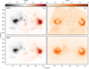 |
Fig. 2. Magnetic field components B∥ (left) and B⊥ (right) from the WFA (top row) and from the MHS model (bottom row), averaged over the equivalent height range (as determined from the column mass) to which the WFA is expected to be sensitive. To allow a direct comparison between the WFA and MHS results, the panels in each column have been clipped to the same values: between [ − 1.35, 1.25] kG for B∥ and [0, 1] kG for B⊥. In addition, the B∥ panels (left column) have been gamma-adjusted to improve visibility of weaker features. |
Qualitatively, the strongest field concentrations both in B∥ and B⊥ agree well, but much of the substructure that the WFA recovers in the superpenumbra of both sunspots, for example, appears more as a homogeneous and comparatively weaker-field haze in the MHS panels. For instance, the strong B∥ inside the sunspots is more extended in the WFA results, especially for the positive-polarity sunspot, and elongated strong-field concentrations are seen to extend radially from both sunspots in the WFA B⊥ that are entirely absent in the MHS.
The stronger field concentrations outside the sunspots in the WFA B∥ are only recovered in location in the MHS B∥, but they are weaker in strength and hardly recovered in terms of fine structure. The lack of magnetic features outside the sunspots in the MHS model is particularly striking when the two B⊥ panels are compared (right column), although much of the fine structure in the WFA B⊥ in the lower left of the FOV (i.e. left of X = 80″ and below Y = −280″) is likely spurious, as suggested by weak total linear polarisation in these areas. The MHS B⊥ field therefore successfully identifies locations with a significant horizontal chromospheric field. Another feature of interest is the band of negative B∥ (the light grey band embedded in the reddish background) around (X, Y) = (110″, −270″) in the WFA panel, which coincides with dark elongated fibrils as seen in the Ca II line core (see e.g., the top left panel of Fig. 1). While it is only weakly visible because its field strength is far weaker than that of the sunspots, it is evidently absent in the MHS panel. We consider these high fibrils in further detail in Sect. 4.3.2.
Figure 3 compares the WFA and MHS magnetic field components quantitatively in two-dimensional histograms. For B∥ (left panel), the correlation is generally tight, as is also shown by the Pearson correlation number of 0.97, and for weak field strengths (below 0.2–0.3 kG), this correlation appears to be essentially one to one. For larger field strengths, the scatter cloud widens and tends to lower field strengths in the MHS compared to the WFA overall, as indicated by the linear regression (dashed red line), which has a slope of 0.84. For B⊥ (right panel), the scatter cloud is much wider. While the WFA-recovered field strengths are generally larger than in the MHS model (i.e. the darkest parts of the two-dimensional histogram are found right of the one-to-one line), there is an extended cloud of points at WFA field strengths below 0.5 kG that exceed that value by some 0.35–0.70 kG in the MHS model. These points correspond to the spuriously looking narrow field enhancements in both sunpsot centres in the MHS B⊥ map. Careful examination of the data suggests that these regions appear as a result of data processing and become pronounced only after averaging in height. Despite the wider scatter and offset by about +100 G in favour of the WFA, the linear regression has a slope of 0.96, indicating an essentially 1:1 relation between the WFA and MHS in B⊥.
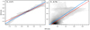 |
Fig. 3. Two-dimensional histograms of the WFA vs. MHS magnetic field for B∥ (left) and B⊥ (right) for the overlapping part of the FOV shown in Fig. 2 (i.e. excluding pixels without Ca II data). The diagonal blue line indicates a 1:1 relation, and the dashed red line shows a linear fit to the data. The numbers between parantheses indicate the respective Pearson correlation coefficients. |
4.2. Chromospheric field azimuth and fibril orientation
As the chromosphere is a low-β regime where the magnetic pressure dominates in the pressure balance, the fibrils visible in the Ca II 8542 Å line core, for example, are expected to be relatively well aligned with the local magnetic field vector, even though the extent to which this is the case may vary depending on target and local conditions (e.g., de la Cruz Rodríguez & Socas-Navarro 2011; Schad et al. 2013, 2015; Leenaarts & Carlsson 2015; Zhu et al. 2016; Martínez-Sykora et al. 2016; Asensio Ramos et al. 2017; Jafarzadeh et al. 2017; Bjørgen et al. 2019). Figure 4 shows the azimuth φ derived from the WFA in yellow and from the MHS model in red, overlaid on an unsharp-masked (with radius 0 5) Ca II line-core intensity image of AR 12723. The MHS azimuth was obtained by averaging over the column mass range equivalent to log τ500 = −4.1 to −5.1 (see Sect. 3.5.2). We did not disambiguate the WFA azimuth (see also Sect. 3.3) and are primarily interested in comparing the fibril orientation with the field azimuth, therefore we omit all arrowheads in Fig. 4 overlays.
 |
Fig. 4. Comparison of fibril orientation and chromospheric field azimuth from the spatially-regularised WFA and the MHS model. The background Ca II 8542 Å image has been unsharp masked with a radius of 0 |

In the full FOV (panel a of Fig. 4), the WFA azimuth agrees well with both the MHS azimuth and the orientation of fibrillar structures in the superpenumbra of both sunspots, as well as with the fibrils in parts of the inter-spot region (e.g., above and to the right of box C). Farther away from the sunspot centres and the stronger field-concentrations and pores, the WFA azimuth disagrees more often with the fibril orientation. Instances of this can be seen in part of the superpenumbra of the negative-polarity sunspot (above and to the very left of box B), in the fibrils connected to the bright plage south of this spot (to the lower left of box D), and in the dark fibril around (X, Y) = (128″, −245″) located to the north of the positive-polarity sunspot. In contrast, the MHS azimuth is relatively well aligned with the fibrils at greater distance from the sunspots as well (especially around the left-hand negative-polarity sunspot and the dark fibril north of the positive-polarity sunspot), which in turn means that the WFA and MHS azimuth cross more often at nearly perpendicular angles. At the same time, the orientation of a long fibril that extends from the positive-polarity sunspot into panel c appears not to be captured in the MHS model (the azimuth bars are essentially parallel to the x-axis), while the WFA azimuth is better aligned with this fibril in several places. Finally, outside the strong-field areas of the active region (e.g., at the bottom and in the lower right and upper left parts of the mosaic FOV) the WFA azimuth is more random, but the lack of clear fibrillar structures also renders a comparison in these regions less straightforward. One source of this randomness is that the WFA will always provide an azimuth as output, even when the linear polarization signal is completely dominated by noise.
Panels b–d of Fig. 4 zoom in on three cutout boxes of about 16″ × 16 marked B–D in Fig. 4a. Cutout B covers part of the negative-polarity sunspot and its superpenumbra, as well as the ROI 1 box (indicated by dashed white lines), cutout C covers a magnetic concentration in the inter-spot region (including ROIs 2 and 3), and cutout D shows the superpenumbra south of the negative-polarity sunspot (including ROI 4). These detailed views paint a similar picture as the FOV overview: the WFA azimuth is often well-aligned with Ca II fibrils at or in the vicinity of strong fields (e.g., dark fibrils close to the sunspot in cutout B, fibrils extending to the south from the positive-polarity pore around (X, Y) = (94″, −270″), and fibrils that cross the lower right quadrant of the box (between about (X, Y) = (93″, −278″) and (X, Y) = (106″, −269″) in cutout C, in the upper left part of cutout D (between (X, Y) = (80″, −270″) and in the upper left corner). The misalignment increases away from sunspot or pore, however (e.g., top 3″ of cutout B, fibrils north of the pore in cutout C, and most of cutout D except for the upper left quadrant). In contrast, the MHS azimuth traces the fibrils over larger parts of these sub-FOVs more often, with the notable exception of the long dark fibrils crossing the lower right quadrant of cutout C, as described before.
4.3. Detailed comparison of selected regions of interest
4.3.1. ROI 1: Sunspot vicinity
Figure 5 presents a comparison of the observations, inversions, and modelling results for the detailed view of ROI 1, just north of the negative polarity sunspot. The first eight columns compare the intensity maps in all four Stokes components from the observations and best fits as determined by the non-LTE inversions and serve primarily to assess the quality of the inferred model atmosphere. The remaining nine columns show the B∥, B⊥, and φ from the MHS model, WFA, and non-LTE STiC inversions. The contours in all panels highlight the regions in which the WFA-derived B⊥ reaches 150 G (solid contours) and 350 G (dashed). As the ROI was rotated counter-clockwise by 90°, the solar X-axis lies along the vertical axis and the sunspot lies to the right of these cut-outs, up to about X = 74″.
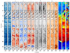 |
Fig. 5. Maps of Stokes intensity and magnetic field components for ROI 1. The ROI has been rotated by 90° counter-clockwise to allow for an identical layout as Figs. 7, A.1, and A.3. The first eight columns contain the Stokes I, Q, U, and V intensity maps, where each column pair first shows the observed and then the synthetic maps, clipped to the same values. The Stokes I map is taken at Ca II 8542 Å line centre, while the other Stokes components are shown at Δλ = +0.21 Å offset. The remaining nine columns contain the magnetic field components B∥, B⊥, and azimuth φ, where each column triple shows the MHS, WFA, and non-LTE inversion result from left to right, again clipped to the same values. The non-LTE magnetic field components are the average over log τ500 = [ − 5.1, −4.1], and the MHS field components are averaged over the equivalent z-height (determined per pixel). The contours highlight regions in which the WFA-derived B⊥ transitions 150 G (solid) and 350 G (dashed). The tick spacing is the same for the x- and y-axes. |
The magnetic field maps were averaged over log τ500 = −4.1 and −5.1 because inspection of the response functions of Ca II Stokes Q, U and V indicates maximum sensitivity to the magnetic field in that log τ500-depth range. The MHS maps are averaged over the equivalent range in column mass, as derived from the non-LTE inversions (see Sect. 3.5.2).
Comparison of the observed and synthetic maps shows that especially Stokes I and in general also V are well reproduced. The synthetic map for V contains locations in which the strong signal is more extended than in the observations (e.g., the blue patch around X = 66″), but also places in which signal is lacking (e.g., around X = 72″). This translates into B∥ maps that in their general distribution of field concentrations are essentially the same for the MHS model, the WFA results, and the non-LTE inversions. However, the WFA and especially the non-LTE inversions return a stronger field in the chromosphere, for example, close to the sunspot (between X = 66″ and 73″) and between X = 80″ and 82″.
The non-LTE inversions do not fit Stokes Q and U as well as V, mostly where the horizontal field is expected to be weak (based on the WFA). For instance, the synthetic maps hardly recover any signal within the contour lines centred at  , where the WFA-derived B⊥ is lower than 150 G, and in general above
  , even though the observed maps clearly exhibit some structure. This is reflected in the inferred B⊥ and φ maps, which are particularly noisy between X = 75″ and 83″.
Figure 6 shows vertical cuts in B∥ and B⊥ along the long axis of ROI 1, averaged over the central 5 pixels across this axis, for the non-LTE-inferred field and the MHS field. The dashed lines indicate the equivalent log τ500 = −4.1 and −5.1 depths over which the field has been averaged for display in Fig. 5, where the log τ500 = −5.1 depth is more corrugated than log τ500 = −4.1, especially in the inversions (upper row). The two B∥ and B⊥ cuts look very similar between the non-LTE inversions and the MHS model. B∥ field concentrations are rooted at z = 0 Mm around X = 68″, 70 5 and 82″, although the non-LTE inversions show that the strong field extends farther and persists between about 0.6–1.2 Mm, while the MHS field exhibits a much more diffuse distribution at these heights. Similarly, the B⊥ cuts have a pair of stronger field concentrations around
  and 82″ that in both cases extend up to about z = 0.6 Mm in the non-LTE panel and slightly lower in the MHS panel. The marked difference is a stronger transverse field above 0.5 Mm between X = 65″ and 67″ for the non-LTE inversions that is absent in the MHS model. Finally, the lower atmosphere (up to about 0.5–0.6 Mm in the non-LTE case and up to about 1 Mm in the MHS case) between X = 74″ and 79″ exhibits almost zero B∥ and B⊥ field strengths in the inversions and in the MHS model.
 |
Fig. 6. Vertical cuts in B∥ (left column) and B⊥ (right column). The cuts have been taken along the long axis of ROI 1, averaging over the central 5 pixels across that axis. Top row: non-LTE-inferred field. Bottom row: MHS field. The non-LTE and MHS panels have been clipped to the same values according the colour bars at the top of the figure. The dashed lines indicate the heights corresponding to log τ500 = −5.1 (upper line) and −4.1 (lower line) in the upper panels and the equivalent column mass in the MHS model in the lower panels. The lower panels also show the field over a larger z-height range than in the top row. |
4.3.2. ROI 3: High fibrils
Figures 7 and 8 present the results for ROI 3 in the same format as Figs. 5 and 6 for ROI 1. The location for ROI 3 was chosen for its crossing of a set of the longest fibrils in our mosaic observations, which are evident as dark slanted bands around Y = −272″ in Stokes I (Fig. 7, first two columns). Stokes V is particularly strong at the location of these fibrils, which is reflected in an apparently homogeneous band of strong negative polarity in the WFA- and non-LTE-inferred B∥ maps. While both Stokes Q and U show structure in their signature at this location, the correlation with the dark bands in Stokes I is not evident. Still, the WFA recovers B⊥ in excess of 150 G in a patch overlapping with the strongest negative B∥ at the location of these fibrils (see the contours at Y = −272″).
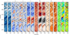 |
Fig. 7. Maps of Stokes intensity and magnetic field components for ROI 3. The format is the same as for Fig. 5, but contours are only shown for B⊥ = 150 G in the WFA-derived field. |
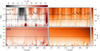 |
Fig. 8. Vertical cuts in B∥ (left column) and B⊥ (right column) for ROI 3. The format is the same as for Fig. 6, but the B⊥ panels (right column) have been clipped individually, according to the colour bars on the right of the figure. |
The non-LTE inversions struggle to reproduce the Q and U profiles in the areas in which the WFA already suggests that the transverse field is weaker, as expected (see the B⊥ = 150 G contours, e.g. between  and −272
 5 and between Y = −272″ and Y = −269″), while the stronger field contour-enclosed areas typically show a similar amount of structure between the observed and synthetic Q and U maps. The non-LTE B⊥ still agrees qualitatively with the WFA-inferred B⊥ B⊥ for most of the sub-FOV, albeit with more noise. The same holds for the azimuth φ, with the exception of several smaller patches that are found in either the WFA or non-LTE inversions (e.g., the blue-red patch at
  in the WFA azimuth that is poorly defined in the non-LTE results).
One stark difference in the comparison of the field for the different methods is that the MHS results show little to no field structuring at the log τ500 equivalent heights that were used to construct these maps, in contrast to ROI 1 (and to some extent, also ROI 2; see Appendix A.1). In particular, the strong B∥ (and to a certain extent, B⊥) associated with the dark fibrils in the Ca II line core intensity image is absent in the MHS model, and the MHS field components instead exhibit little to no structure. These discrepancies are also reflected in the vertical cross-cuts shown in Fig. 8, where at the height of the horizontal cuts (i.e. between the dashed lines) the MHS model exhibits a weakly positive B∥ of less than 30 G and B⊥ below 80 G in the strongest-field part around Y = −266″. While at the equivalent log τ500 depths the non-LTE-inferred B∥ is only barely stronger in absolute terms than the MHS results, B⊥ is stronger by up to a factor 5 in the top right non-LTE panel.
Lower down in the atmosphere, below 500 km, the alternating positive and negative B∥ polarities in the MHS panel, and in particular, their extensions to 700–800 km, are not always as well recovered in the non-LTE results. However, careful inspection shows that most of the stronger-field concentrations at heights 0–200 km are located at approximately the same place in both panels, but typically with larger field strengths in the non-LTE case: the positive polarities at  , −272
 5, between −271
 5 and −271″, and between −268
 5 and −268″, or the negative polarities at Y = −276″, near −274″ and −267
 7.
7.
A similar structuring of alternating stronger and weaker B⊥ along the vertical cut is found in the lower atmosphere of the MHS model, while the non-LTE cut only shows the stronger concentrations of these, for example at −273 5, −269″ and −266″. The inversions of Fe I struggled, especially for Stokes Q and U. Higher up in the atmosphere, above about 1 Mm, the results diverge even further, with a B⊥ concentration in excess of 300 G in the non-LTE panel around Y = − 276″, while the MHS B⊥ is a factor 5–6 weaker at an equivalent column mass. On the other hand, the B⊥ values in the upper right corner differ by only up to a factor 2 and are often even quite close between non-LTE and MHS results.
5. Discussion
5.1. Chromospheric magnetic field on active region scales
Qualitatively, the MHS and WFA field agree in spatial distribution of the stronger-field concentrations, that is, sunspots and pores, but the WFA shows a more enhanced field fine-structure (see Fig. 2), which can be most clearly seen for the transverse component in the superpenumbra of either sunspot. While a contribution from the photosphere could conceivable play a role, it is unlikely the case here as both Stokes Q and U exhibit this strong-signal superpenumbral fine-structure already in the first off-core wavelength samplings, and the restricted wavelength range chosen to determine the WFA would furthermore minimise any photospheric contribution.
Quantitatively, B∥ exhibits a tighter correlation between the WFA and MHS model than B⊥, while the latter is closer to a one-to-one relation. The WFA field strengths tend to be larger than in the MHS model in both cases, however. This tendency can easily be understood by considering the maps in Fig. 2, which show a much more extended region of strong-field B∥ for the sunspots in the WFA map than in the MHS map, especially for the positive-polarity sunspot. Similarly, the strongest enhancements in B⊥ are found for the superpenumbral substructure in the WFA map, while the MHS exhibits a much smoother spatial distribution. The spatial distribution has no counterpart in the WFA map, which explains the scatter cloud at the top left of the right-hand panel in Fig. 3, while the superpenumbral substructure causes the majority of the distribution to lie to the right of the one-to-one diagonal.
On large scales, the MHS azimuth appears to follow the Ca II 8542 Å fibril structures more closely than the WFA azimuth does. This is particularly so outside the sunspots and pores. The Ca II Stokes Q and U signals are weak and noisy there, leading to weaker and more uncertain inferred transverse field strengths and azimuths. The visible misalignment between fibrils and WFA azimuth could therefore, at least in part, be attributable to the signal-to-noise ratio of the underlying observations. However, whether the inferred field should follow the line-core fibril structures may depend on the target. For instance, de la Cruz Rodríguez & Socas-Navarro (2011) found most of the derived azimuths to be consistent with the fibril orientation in two targets observed with Ca II 8542 Å spectropolarimetry. Similarly, Schad et al. (2013) found the inferred field orientation to be well aligned with the projected angles of the fibrils, to within an error of only 10°, and Asensio Ramos et al. (2017) reported an alignment to within about 16° for the superpenumbra, although the misalignment could be up to about 34° in magnetically weaker plage regions. We observe a qualitatively similar effect in that the WFA azimuth appears to trace the dark superpenumbral fibrils reasonably well, but differs more often with fibrils outside the stronger-field concentrations.
5.2. Magnetic field from non-LTE inversions
In general, the non-LTE inversions recover a similar spatial distribution of the chromospheric field as the WFA, in particular for the B∥ component, but to a decent extent also for B⊥ (at least where the transverse field is relatively strong). The inversions struggle to derive clean maps for B⊥ wherever Stokes Q and/or U are relatively noisy, however, as expected (e.g., ROIs 3 and 4 in Figs. 7 and A.3, respectively). Although the spatially regularised WFA served as initial guess, the B⊥ maps for ROIs 3 and 4 (and in part also ROI 2) are far from smooth. This carries over into the non-LTE-inferred azimuth, which for most of these FOVs disagrees with the WFA-derived azimuth even in a broad sense (see Figs. A.1 and A.3 for ROIs 2 and 4, respectively). One reason for the increased noise is that in order for non-LTE inversions to work, the stratification must be inferred correctly for all parameters, not only for the magnetic field. This leads to more degenerate solutions and hence to more noise in the inferred parameters.
Of all ROIs, the ROI 1 shows the highest degree of similarity in the MHS, WFA, and non-LTE inversions for all three magnetic field components. ROI 2 comes a close second, at least for B∥ and B⊥, and ROIs 3 and 4 differ considerably in most aspects. While all four ROIs exhibit similar photospheric patterns in the MHS model and non-LTE inversions in the vertical cross-cuts for B∥ and B⊥, the MHS B⊥ field strengths in ROIs 3 and 4 are up to a factor of 5 smaller at chromospheric heights than what the non-LTE inversions indicate. This can be understood from the proximity to strong-field concentrations for ROIs 1 and 2, which persists from the photosphere to greater heights (see the vertical cross-cuts in Figs. 6 and A.2), in contrast to ROIs 3 and 4, which are located in more quiet parts of the FOV. The MHS model extrapolates from the photospheric field, therefore it will inherently exhibit a better agreement at chromospheric heights in the vicinity of strong-field concentrations than in magnetically weaker regions.
Furthermore, despite the large difference in transverse chromospheric field strengths in the quiet ROIs, the distribution of weaker field in the photosphere and stronger field in the chromosphere is qualitatively similar in the MHS model and non-LTE inversions. This pattern can be explained by the difference in origin of the field. In the lower atmosphere, the field comes from the (weak) photospheric polarities, while the field higher up connects the main polarities of the active region. The MHS model and non-LTE inversions therefore present a similar magnetic field stratification of the active region connectivity, but the non-LTE inversion recovers the stronger transverse field in the chromosphere.
Evidently, ROI 3 presents a further discrepancy that cannot be explained in a similar way. Here, both the WFA and non-LTE inversions detect the enhanced Ca II 8542 Å Stokes polarisation that corresponds to the dark fibrils traversing this sub-field, while the MHS model essentially shows a smooth extension from the upper-photosphere field state. Although these dark fibrils appear to connect the two sunspots and are thus expected to be rooted in either of the main polarities in the photosphere, the MHS model is unable to reproduce the magnetic imprint thereof at chromospheric heights.
6. Conclusions
We have presented an analysis of the chromospheric magnetic field in AR 12723 as inferred with a spatially regularised WFA and a non-LTE inversion code. We compared the results with those from a magnetohydrostatic model based solely on the photospheric vector magnetic field. We find that the chromospheric field is qualitatively similar in these methods. The line-of-sight component is best reproduced in the MHS model, while the transverse component is consistently weaker than the WFA-derived field, especially outside the sunspots. In general, the MHS model also presents smoother field component maps than the WFA, despite the spatial regularisation applied in the latter. While the MHS model is unable to recover the magnetic imprint in B∥ and B⊥ from a set of long fibrils that appear to connect the two sunspots, the agreement with the WFA is otherwise remarkably good.
In addition, the vertical cuts in magnetic field offer a similar view in the MHS model and non-LTE inversions, especially for the two ROIs that are close to the stronger field concentrations (i.e. the negative-polarity sunspot and crossing the pores) and at least qualitatively for the ROIs that are taken in more quiet parts of the field of view. In some places, the transverse field strengths are up to a factor of 5 or so weaker than in the non-LTE inversions or WFA, however. On the other hand, the non-LTE inversions struggle to recover the transverse component when its strength is below some 200–300 G. For the more quiet ROIs, the non-LTE inversions also appear to overshoot and settle on stronger B⊥ than the WFA indicates, even though the Stokes Q and U are not always recovered in magnitude. The noisiness of the non-LTE-inferred B⊥ and φ maps in contrast to those from the spatially regularised WFA further emphasise the need for spatial coupling in the inversions, as proposed recently by Asensio Ramos & de la Cruz Rodríguez (2015), de la Cruz Rodríguez (2019).
While the MHS model agrees qualitatively (and to a large extent, also quantitively) with the observationally inferred chromospheric field, it does not retrieve all the features from the observations. Our results therefore support earlier studies, which indicate that including a chromospheric constraint in field extrapolations or data-driven modelling can improve the recovery of chromospheric and coronal magnetic structures. In particular, the difficulty of reaching a transverse chromospheric field strength similar to that which is observationally inferred or of recovering the presence of high fibrils suggests that key ingredients may thus still be missing. An accurate estimate of the chromospheric field within, for instance, erupting flux ropes is vital to properly predict the geo-effectiveness of earth-bound CMEs, however (Kilpua et al. 2019).
The Synoptic Optical Long-term Investigations of the Sun (SOLIS; Keller et al. 2003) Vector Spectromagnetograph did provide near-daily full-disk line-of-sight chromospheric magnetograms using Ca II 8542 Å until late October 2017, but has not been operational since.
See the remap utility package in https://github.com/ISP-SST/ISPy
Acknowledgments
G.V. has been supported by a grant from the Swedish Civil Contingencies Agency (MSB). This research has received funding from the European Union’s Horizon 2020 research and innovation programme under grant agreement No. 824135. J.L. and S.D. are supported by a grant from the Knut and Alice Wallenberg foundation (2016.0019). X.Z. is supported by the mobility program (M-0068) of the Sino-German Science Center. This project has received funding from the European Research Council (ERC) under the European Union’s Horizon 2020 research and innovation programme (SUNMAG, grant agreement 759548). This project has received funding from the European Research Council (ERC) under the European Union’s Horizon 2020 research and innovation programme (SolMAG, grant agreement No. 724391). The Institute for Solar Physics is supported by a grant for research infrastructures of national importance from the Swedish Research Council (registration number 2017-00625). The Swedish 1-m Solar Telescope is operated on the island of La Palma by the Institute for Solar Physics of Stockholm University in the Spanish Observatorio del Roque de los Muchachos of the Instituto de Astrofísica de Canarias. The SDO/HMI data used are courtesy of NASA/SDO and HMI science team. The inversions were performed on resources provided by the Swedish National Infrastructure for Computing (SNIC) at the National Supercomputer Centre at Linköping University. We made much use of NASA’s Astrophysics Data System Bibliographic Services. Last but not least, we acknowledge the community effort to develop open-source packages used in this work: numpy (Oliphant 2006; numpy.org), matplotlib (Hunter 2007; matplotlib.org), scipy (Virtanen et al. 2020; scipy.org), astropy (Astropy Collaboration 2013, 2018; astropy.org), sunpy (The SunPy Community 2020; sunpy.org), scikit-learn (Pedregosa et al. 2011; scikit-learn.org).
References
- Asensio Ramos, A., & de la Cruz Rodríguez, J. 2015, A&A, 577, A140 [NASA ADS] [CrossRef] [EDP Sciences] [Google Scholar]
- Asensio Ramos, A., de la Cruz Rodríguez, J., Martínez González, M. J., & Socas-Navarro, H. 2017, A&A, 599, A133 [NASA ADS] [CrossRef] [EDP Sciences] [Google Scholar]
- Astropy Collaboration (Robitaille, T. P., et al.) 2013, A&A, 558, A33 [NASA ADS] [CrossRef] [EDP Sciences] [Google Scholar]
- Astropy Collaboration (Price-Whelan, A. M., et al.) 2018, AJ, 156, 123 [Google Scholar]
- Bjørgen, J. P., Leenaarts, J., Rempel, M., et al. 2019, A&A, 631, A33 [Google Scholar]
- Bobra, M. G., Sun, X., Hoeksema, J. T., et al. 2014, Sol. Phys., 289, 3549 [Google Scholar]
- de la Cruz Rodríguez, J. 2019, A&A, 631, A153 [NASA ADS] [CrossRef] [EDP Sciences] [Google Scholar]
- de la Cruz Rodríguez, J., & Piskunov, N. 2013, ApJ, 764, 33 [Google Scholar]
- de la Cruz Rodríguez, J., & Socas-Navarro, H. 2011, A&A, 527, L8 [NASA ADS] [CrossRef] [EDP Sciences] [Google Scholar]
- de la Cruz Rodríguez, J., Rouppe van der Voort, L., Socas-Navarro, H., & van Noort, M. 2013, A&A, 556, A115 [NASA ADS] [CrossRef] [EDP Sciences] [Google Scholar]
- de la Cruz Rodríguez, J., Löfdahl, M. G., Sütterlin, P., Hillberg, T., & Rouppe van der Voort, L. 2015, A&A, 573, A40 [NASA ADS] [CrossRef] [EDP Sciences] [Google Scholar]
- de la Cruz Rodríguez, J., Leenaarts, J., & Asensio Ramos, A. 2016, ApJ, 830, L30 [Google Scholar]
- de la Cruz Rodríguez, J., Leenaarts, J., Danilovic, S., & Uitenbroek, H. 2019, A&A, 623, A74 [Google Scholar]
- De Rosa, M. L., Schrijver, C. J., Barnes, G., et al. 2009, ApJ, 696, 1780 [NASA ADS] [CrossRef] [Google Scholar]
- Díaz Baso, C. J., de la Cruz Rodríguez, J., & Danilovic, S. 2019, A&A, 629, A99 [NASA ADS] [CrossRef] [EDP Sciences] [Google Scholar]
- Fleishman, G., Mysh’yakov, I., Stupishin, A., Loukitcheva, M., & Anfinogentov, S. 2019, ApJ, 870, 101 [NASA ADS] [CrossRef] [Google Scholar]
- Hammerschlag, R. H., Sliepen, G., Bettonvil, F. C. M., et al. 2013, Opt. Eng., 52, 081603 [NASA ADS] [CrossRef] [Google Scholar]
- Harvey, J. W. 2012, Sol. Phys., 280, 69 [NASA ADS] [CrossRef] [Google Scholar]
- Henriques, V. M. J. 2012, A&A, 548, A114 [NASA ADS] [CrossRef] [EDP Sciences] [Google Scholar]
- Hunter, J. D. 2007, Comput. Sci. Eng., 9, 90 [NASA ADS] [CrossRef] [Google Scholar]
- Jafarzadeh, S., Rutten, R. J., Solanki, S. K., et al. 2017, ApJS, 229, 11 [CrossRef] [Google Scholar]
- Jin, M., Schrijver, C. J., Cheung, M. C. M., et al. 2016, ApJ, 820, 16 [NASA ADS] [CrossRef] [Google Scholar]
- Keller, C. U., Harvey, J. W., & Giampapa, M. S. 2003, in Innovative Telescopes and Instrumentation for Solar Astrophysics, eds. S. L. Keil, & S. V. Avakyan, SPIE Conf. Ser., 4853, 194 [Google Scholar]
- Kilpua, E. K. J., Lugaz, N., Mays, M. L., & Temmer, M. 2019, Space Weather, 17, 498 [NASA ADS] [CrossRef] [Google Scholar]
- Kleint, L. 2017, ApJ, 834, 26 [Google Scholar]
- Leenaarts, J., Carlsson, M., & Rouppe van der Voort, L. 2015, ApJ, 802, 136 [NASA ADS] [CrossRef] [Google Scholar]
- Leka, K. D., Barnes, G., & Crouch, A. 2014, Astrophysics Source Code Library [record ascl:1404.007] [Google Scholar]
- Lemen, J. R., Title, A. M., Akin, D. J., et al. 2012, Sol. Phys., 275, 17 [Google Scholar]
- Löfdahl, M. G., Hillberg, T., de la Cruz Rodriguéz, J., et al. 2021, A&A, 653, A68 [NASA ADS] [CrossRef] [EDP Sciences] [Google Scholar]
- Martínez-Sykora, J., De Pontieu, B., Carlsson, M., & Hansteen, V. 2016, ApJ, 831, L1 [CrossRef] [Google Scholar]
- Metcalf, T. R. 1994, Sol. Phys., 155, 235 [Google Scholar]
- Metcalf, T. R., De Rosa, M. L., Schrijver, C. J., et al. 2008, Sol. Phys., 247, 269 [Google Scholar]
- Morosin, R., de la Cruz Rodríguez, J., Vissers, G. J. M., & Yadav, R. 2020, A&A, 642, A210 [NASA ADS] [CrossRef] [EDP Sciences] [Google Scholar]
- Oliphant, T. E. 2006, A guide to NumPy (USA: Trelgol Publishing), 1 [Google Scholar]
- Pedregosa, F., Varoquaux, G., Gramfort, A., et al. 2011, J. Mach. Learn. Res., 12, 2825 [Google Scholar]
- Pesnell, W. D., Thompson, B. J., & Chamberlin, P. C. 2012, Sol. Phys., 275, 3 [Google Scholar]
- Pietarila, A., Socas-Navarro, H., & Bogdan, T. 2007, ApJ, 663, 1386 [Google Scholar]
- Pietrow, A. G. M., Kiselman, D., de la Cruz Rodríguez, J., et al. 2020, A&A, 644, A43 [NASA ADS] [CrossRef] [EDP Sciences] [Google Scholar]
- Piskunov, N., & Valenti, J. A. 2017, A&A, 597, A16 [NASA ADS] [CrossRef] [EDP Sciences] [Google Scholar]
- Price, D. J., Pomoell, J., & Kilpua, E. K. J. 2020, A&A, 644, A28 [NASA ADS] [CrossRef] [EDP Sciences] [Google Scholar]
- Reardon, K. P., & Cauzzi, G. 2012, Am. Astron. Soc. Meeting Abstr., 220, 201.11 [NASA ADS] [Google Scholar]
- Schad, T. A., Penn, M. J., & Lin, H. 2013, ApJ, 768, 111 [NASA ADS] [CrossRef] [Google Scholar]
- Schad, T. A., Penn, M. J., Lin, H., & Tritschler, A. 2015, Sol. Phys., 290, 1607 [NASA ADS] [CrossRef] [Google Scholar]
- Scharmer, G. 2017, SOLARNET IV: The Physics of the Sun from the Interior to the Outer Atmosphere, 85 [Google Scholar]
- Scharmer, G. B., Bjelksjo, K., Korhonen, T. K., Lindberg, B., & Petterson, B. 2003, in The 1-meter Swedish solar telescope, eds. S. L. Keil, & S. V. Avakyan, SPIE Conf. Ser., 4853, 341 [NASA ADS] [Google Scholar]
- Scharmer, G. B., Narayan, G., Hillberg, T., et al. 2008, ApJ, 689, L69 [Google Scholar]
- Scherrer, P. H., Schou, J., Bush, R. I., et al. 2012, Sol. Phys., 275, 207 [Google Scholar]
- Schou, J., Scherrer, P. H., Bush, R. I., et al. 2012, Sol. Phys., 275, 229 [Google Scholar]
- Scullion, E., Rouppe van der Voort, L., Wedemeyer, S., & Antolin, P. 2014, ApJ, 797, 36 [Google Scholar]
- Shine, R. A., Title, A. M., Tarbell, T. D., et al. 1994, ApJ, 430, 413 [NASA ADS] [CrossRef] [Google Scholar]
- The SunPy Community (Barnes, W. T., et al.) 2020, ApJ, 890, 68 [Google Scholar]
- Toriumi, S., Takasao, S., Cheung, M. C. M., et al. 2020, ApJ, 890, 103 [NASA ADS] [CrossRef] [Google Scholar]
- Uitenbroek, H. 2001, ApJ, 557, 389 [Google Scholar]
- van Noort, M., Rouppe van der Voort, L., & Löfdahl, M. G. 2005, Sol. Phys., 228, 191 [Google Scholar]
- Virtanen, P., Gommers, R., Oliphant, T. E., et al. 2020, Nat. Methods, 17, 261 [Google Scholar]
- Vissers, G., & Rouppe van der Voort, L. 2012, ApJ, 750, 22 [Google Scholar]
- Vissers, G. J. M., Danilovic, S., de la Cruz Rodríguez, J., et al. 2021, A&A, 645, A1 [NASA ADS] [CrossRef] [EDP Sciences] [Google Scholar]
- Wiegelmann, T. 2004, Sol. Phys., 219, 87 [NASA ADS] [CrossRef] [Google Scholar]
- Wiegelmann, T., Inhester, B., & Sakurai, T. 2006, Sol. Phys., 233, 215 [Google Scholar]
- Wiegelmann, T., Thalmann, J. K., Schrijver, C. J., De Rosa, M. L., & Metcalf, T. R. 2008, Sol. Phys., 247, 249 [NASA ADS] [CrossRef] [Google Scholar]
- Zhu, X., & Wiegelmann, T. 2018, ApJ, 866, 130 [NASA ADS] [CrossRef] [Google Scholar]
- Zhu, X., & Wiegelmann, T. 2019, A&A, 631, A162 [NASA ADS] [CrossRef] [EDP Sciences] [Google Scholar]
- Zhu, X., Wang, H., Du, Z., & He, H. 2016, ApJ, 826, 51 [NASA ADS] [CrossRef] [Google Scholar]
- Zhu, X., Wiegelmann, T., & Solanki, S. K. 2020, A&A, 640, A103 [NASA ADS] [CrossRef] [EDP Sciences] [Google Scholar]
Appendix A: Other regions of interest
In this appendix we present the results for additional regions of interest in similar format as for ROIs 1 and 3.
A.1. ROI 2: Pore and strong-field concentrations
Fig. A.1 and A.2 present the results for ROI 2 in a similar format as Figs. 5 and 6, but the contours in Fig. A.1 now solely indicate the B⊥ = 150 G level. Similar to ROI 1, Stokes I and V are best reproduced in general, while Q and U are more problematic, especially where the WFA already indicates that the field is weak. For instance, the regions to the right of the contours around (X, Y) = (95″, −266″), the band around Y = −264″, or within the contours around  are mostly devoid of signal in the synthetic Q and U maps. Surprisingly, this is also the case for that part of the ROI below the contour around Y = −264″, where the WFA returned stronger B⊥ and a similar result might have been expected as above the contour at Y = −262″ and to the left of those crossing the vertical edges at
  and −257
 5, where much of the structure in linear polarisation is reproduced.
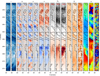 |
Fig. A.1. Maps of Stokes intensity and magnetic field components for ROI 2. The format is the same as for Fig. 5, but the contours now only show the WFA-derived B⊥ = 150 G boundary. |
 |
Fig. A.2. Vertical cuts in B∥ (left column) and B⊥ (right column) for ROI 2 in the same format as Fig. 6. |
This ROI crosses a positive-polarity pore around Y = −267″ and another stronger field concentration around Y = −256″, as is evident from the B∥ maps in Figs. A.1 and A.2. Especially around the pore, the MHS, WFA and non-LTE inversions agree in the top-down viewed shape of the positive polarity, although the non-LTE inversions suggest a much stronger field at these heights than either the WFA and especially the MHS results. Moreover, where the WFA and non-LTE inversions return strong negative B∥ (i.e. around Y = −258″ and especially −256″), there is no such significant concentration in the MHS model. When we searched for the same locations in the vertical cut, we found that the MHS model does have marked B∥ field concentrations at these Y locations, but they are already strongly attenuated at heights equivalent to log τ500 = −4.1 (lower dashed line) and field strengths of some 500–600 G above the pore and −100 G around Y = −256″. In contrast, the non-LTE inversions have field strengths of about 800 G and −200 G that persist above v = −4.1. In both cases, B∥ is strongly vertical above the positive polarity pore, but somewhat more inclined with height in the MHS model for the negative polarity.
The transverse field shows the strongest concentrations at the location of the pore. It only extends a few hundred kilometers in height in the MHS model and is reduced to some 200–300 G between the log τ500 = −4.1 and −5.1 lines, while the non-LTE inversions exhibit B∥ in excess of 400 G around  . For most of the vertical cut, the non-LTE inversions and MHS model exhibit a weak B⊥ field.
While the azimuth for ROI 1 is largely similar in the MHS, WFA, and non-LTE inversions for most of this sub-FOV, this is not the case for ROI 2 (last three columns of Fig. A.1). Although we find some resemblance between MHS and WFA azimuths south of about Y = −268″, only a few other spots in the FOV are anywhere near agreement (e.g., close to  , −258″ , or −254
 5). Noise dominates the non-LTE azimuth, although with some effort, similar patterns as in the WFA azimuth can be found south of Y = −269″, between the contours at
  and −263″, between
  and −258
 5, and north of
  .
.
A.2. ROI 4: Fibrils in the vicinity of sunspots
Finally, Figs. A.3 and A.4 present the results for a region covering some of the longer fibrils that extend to the south-west of the negative-polarity sunspot. Similar to ROI 3, Stokes Q and U are again best reproduced where the WFA indicates B⊥ ≥ 150 G (dark orange within the contours in the middle B⊥ panel), although the magnitude of the signal is not always reproduced (e.g., red in Stokes U at  or blue in the same panel, but around −267
 5). Outside these contours, little signal is found in the synthetic Q and U profiles. This explains the noisiness of B⊥ and φ at these locations. Within the stronger-B⊥ contours, the non-LTE-inferred B⊥ and φ appear more homogeneous, with the former reaching larger field strengths than in the WFA. The corresponding φ panels show largely the same angle in these places, except within the contour at Y = −271″. Interestingly, the non-LTE azimuth much more clearly resembles the WFA results than ROI 2, even though the B⊥ magnitudes of the two ROIs are similar.
The MHS model exhibits a much weaker field throughout, of the order of the weaker field in the WFA cut. Qualitatively, however, it agrees in having stronger B⊥ in the upper part of the ROI, north of about Y = −270″. This is also reflected in the vertical cross-cut (Fig. A.4, right column), showing an area of stronger field in the upper right corner of the cross-cut for the non-LTE inversions and the MHS model. The B⊥ in the lower atmosphere shows little resemblance in the two, however, except maybe the location of a region of stronger B⊥ around Y = −272″, but this has a much smaller extent in the MHS model. Finally, the MHS azimuth φ (Fig. A.3, third column from the right) is very different from that of the WFA or non-LTE inversions.
Stokes V is largely reproduced, except for some of the details around Y = −270″ and −267″, but his seems to have little effect on the determined B∥ when compared to the WFA. The contrast with the MHS B∥ is evident, however. The band of near-zero negative polarity that is recovered in the WFA and non-LTE inversions between  and −271
 5 (correlating with a likewise weakly positive Stokes V signal) is positive in the MHS model, and the stronger negative polarity in the former two around −267″ is barely negative in the MHS model. The vertical cross-cut (Fig. A.4, left column) shows that the reason is a transition from positive to negative polarity where a strong positive field concentration extends over roughly 1 Mm and into the bottom part of the height range used for the maps in Fig. A.3. Moreover, any sign of a band of weak negative B∥ left of
  is missing in the MHS model. On the other hand, the B∥ in the lower atmosphere of the non-LTE inversions bears some similarity to that in the MHS results, at least left of about Y = −270″. Even though they generally disagree in magnitude and often disagree in (vertical) extent as well, the negative polarity concentrations close to Y = −278″, −277
 5, and near −270″, as well as the positive concentrations between
  and −271
 5 or the alternating positive-negative concentrations between
  and −270″ are similar in the two panels.
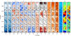 |
Fig. A.3. Maps of Stokes intensity and magnetic field components for ROI 4. The format is the same as for Fig. A.1. |
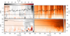 |
Fig. A.4. Vertical cuts in B∥ (left column) and B⊥ (right column) for ROI 4, in the same format as Fig. 8. |
All Tables
Number of nodes used in each inversion cyclefor the temperature T, line-of-sight velocity vlos, and microturbulent velocity vmicro.
All Figures
|
Fig. 1. SST/CRISP mosaic and context SDO/HMI-derived SHARP magnetic field of NOAA AR 12723. Upper left: Ca II 8542 Å line core image. Upper right: Milne-Eddington inferred photospheric Br magnetic field from Fe I 6173 Å observations by SST/CRISP. Lower left: chromospheric radial magnetic field Br from the spatially regularised WFA. Lower right: same as the upper right panel, but from SDO/HMI. The line-of-sight magnetic field maps have been clipped to ±1.5 kG and are all reprojected and mapped to cylindrical equal-area (CEA) coordinates. The mapping to CEA precludes any direct comparison by coordinate of features in the top left panel vs. the other panels. The white boxes in the top left panel indicate narrow regions of interest (ROIs) selected for (non-)LTE inversion and are indicated (approximately, i.e. without mapping distortion) by cyan boxes in the top right and bottom left panels. The dashed green box in the top right panel highlights the FOV selected for the magnetohydrostatic simulation, while the purple contour in the lower right panel traces the SST mosaic field of view. |
| In the text | |
|
Fig. 2. Magnetic field components B∥ (left) and B⊥ (right) from the WFA (top row) and from the MHS model (bottom row), averaged over the equivalent height range (as determined from the column mass) to which the WFA is expected to be sensitive. To allow a direct comparison between the WFA and MHS results, the panels in each column have been clipped to the same values: between [ − 1.35, 1.25] kG for B∥ and [0, 1] kG for B⊥. In addition, the B∥ panels (left column) have been gamma-adjusted to improve visibility of weaker features. |
| In the text | |
|
Fig. 3. Two-dimensional histograms of the WFA vs. MHS magnetic field for B∥ (left) and B⊥ (right) for the overlapping part of the FOV shown in Fig. 2 (i.e. excluding pixels without Ca II data). The diagonal blue line indicates a 1:1 relation, and the dashed red line shows a linear fit to the data. The numbers between parantheses indicate the respective Pearson correlation coefficients. |
| In the text | |
|
Fig. 4. Comparison of fibril orientation and chromospheric field azimuth from the spatially-regularised WFA and the MHS model. The background Ca II 8542 Å image has been unsharp masked with a radius of 0 |
| In the text | |
|
Fig. 5. Maps of Stokes intensity and magnetic field components for ROI 1. The ROI has been rotated by 90° counter-clockwise to allow for an identical layout as Figs. 7, A.1, and A.3. The first eight columns contain the Stokes I, Q, U, and V intensity maps, where each column pair first shows the observed and then the synthetic maps, clipped to the same values. The Stokes I map is taken at Ca II 8542 Å line centre, while the other Stokes components are shown at Δλ = +0.21 Å offset. The remaining nine columns contain the magnetic field components B∥, B⊥, and azimuth φ, where each column triple shows the MHS, WFA, and non-LTE inversion result from left to right, again clipped to the same values. The non-LTE magnetic field components are the average over log τ500 = [ − 5.1, −4.1], and the MHS field components are averaged over the equivalent z-height (determined per pixel). The contours highlight regions in which the WFA-derived B⊥ transitions 150 G (solid) and 350 G (dashed). The tick spacing is the same for the x- and y-axes. |
| In the text | |
|
Fig. 6. Vertical cuts in B∥ (left column) and B⊥ (right column). The cuts have been taken along the long axis of ROI 1, averaging over the central 5 pixels across that axis. Top row: non-LTE-inferred field. Bottom row: MHS field. The non-LTE and MHS panels have been clipped to the same values according the colour bars at the top of the figure. The dashed lines indicate the heights corresponding to log τ500 = −5.1 (upper line) and −4.1 (lower line) in the upper panels and the equivalent column mass in the MHS model in the lower panels. The lower panels also show the field over a larger z-height range than in the top row. |
| In the text | |
|
Fig. 7. Maps of Stokes intensity and magnetic field components for ROI 3. The format is the same as for Fig. 5, but contours are only shown for B⊥ = 150 G in the WFA-derived field. |
| In the text | |
|
Fig. 8. Vertical cuts in B∥ (left column) and B⊥ (right column) for ROI 3. The format is the same as for Fig. 6, but the B⊥ panels (right column) have been clipped individually, according to the colour bars on the right of the figure. |
| In the text | |
|
Fig. A.1. Maps of Stokes intensity and magnetic field components for ROI 2. The format is the same as for Fig. 5, but the contours now only show the WFA-derived B⊥ = 150 G boundary. |
| In the text | |
|
Fig. A.2. Vertical cuts in B∥ (left column) and B⊥ (right column) for ROI 2 in the same format as Fig. 6. |
| In the text | |
|
Fig. A.3. Maps of Stokes intensity and magnetic field components for ROI 4. The format is the same as for Fig. A.1. |
| In the text | |
|
Fig. A.4. Vertical cuts in B∥ (left column) and B⊥ (right column) for ROI 4, in the same format as Fig. 8. |
| In the text | |
Current usage metrics show cumulative count of Article Views (full-text article views including HTML views, PDF and ePub downloads, according to the available data) and Abstracts Views on Vision4Press platform.
Data correspond to usage on the plateform after 2015. The current usage metrics is available 48-96 hours after online publication and is updated daily on week days.
Initial download of the metrics may take a while.